Efficient simulation of non-classical liquid-vapour phase-transition flows: a method of fundamental solutions

Abstract

Classical continuum-based liquid vapour phase-change models typically assume continuity of temperature at phase interfaces along with a relation which describes the rate of evaporation at the interface (Hertz-Knudsen-Schrage, for example). However, for phase transitions processes at small scales, such as the evaporation of nanodroplets, the assumption that the temperature is continuous across the liquid-vapour interface leads to significant inaccuracies (McGaughey & Ward, 2002; Rana et al., 2019), as may the adoption of classical constitutive relations that lead to the Navier-Stokes-Fourier equations (NSF). In this article, to capture the notable effects of rarefaction at small scales, we adopt an extended continuum-based approach utilizing the coupled constitutive relations (CCR). In CCR theory, additional terms are invoked in the constitutive relations of NSF equations originating from the arguments of irreversible thermodynamics as well as consistent with kinetic theory of gases. The modelling approach allows us to derive new fundamental solutions for the linearised CCR model and to develop a numerical framework based upon the method of fundamental solutions (MFS) and enables three-dimensional multiphase micro-flow simulations to be performed at remarkably low computational cost. The new framework is benchmarked against classical results and then explored as an efficient tool for solving three-dimensional phase-change events involving droplets.

1 Introduction

When a liquid evaporates it loses energy; that is why sweating cools us down. Evaporation is an effective cooling mechanism widely employed by nature; for example, as a body-temperature control for mammals (Sherwood, 2005), and in engineering applications, such as spray drying, spray cooling and microelectronics cooling (Dhavaleswarapu et al., 2012; Plawsky et al., 2014; Ling et al., 2014). The use of pot-in-pot coolers by mankind can be tracked back to Bronze Age civilisation (Evans, 2000); a device that relies on the principle of evaporative cooling.

The description of phase-transition processes in micro/nano scales is intriguing, mainly due to the inability of classical continuum theories to accurately capture the rarefied vapour-flow characteristic. Specifically, as the representative physical length scale ($\ell$) of the flow becomes comparable to the mean free path ($\lambda$) in the vapour, i.e., the Knudsen number $(\mathrm{Kn}=\lambda/\ell)\approx 1$ (Bird, 1994; Cercignani, 2000; Sone, 2007; Struchtrup, 2005; Torrilhon, 2016). The classical continuum description based on the Euler or Navier–Stokes–Fourier (NSF) equations is valid only in regimes for which $\mathrm{Kn}\lesssim 0.001$—referred to as the hydrodynamic regime. There are, of course, computational atomistic techniques, such as molecular dynamics simulations (MD), which are capable of modelling phase transition at nano-scales. However, due to computational time and memory limitations, it is impractical to use them for multi-scale processes, which span over a wide range of time and length scales.

The behaviour of a dilute vapour phase can readily be described by the Boltzmann equation, which is an evolution equation for the (velocity) distribution function of vapour molecules (Bird, 1994; Cercignani, 2000). The Boltzmann equation offers the complete mesoscopic description of the vapour for all range of $\mathrm{Kn}$; however, the exact analytical solution of the Boltzmann equation is intractable in a general case while its numerical solutions are computationally very expensive. Grad—in his seminal work (Grad, 1949a, b)—proposed an asymptotic solution procedure for the Boltzmann equation through the method of moment. A variety of other extended fluid dynamics equations, aiming to describe processes under rarefied conditions, have been developed, see e.g. Eu (1992); Müller & Ruggeri (1998); Kremer (2010); Struchtrup (2005); Chakraborty & Durst (2007); Dongari et al. (2010); Myong (2014); Torrilhon (2016). These models close the gap between classical fluid dynamics and kinetic theory; that is, they aim at a good description in the transition regime ($0.001\lesssim\mathrm{Kn}\lesssim 1$).

The classical phase transition models, found in the literature, assume that the temperature and the velocity tangential to the interface are continuous across it. However, it is now well established, both experimentally and theoretically (McGaughey & Ward, 2002; Bond & Struchtrup, 2004; Rana et al., 2019), that such assumptions are invalid at a nano-confined liquid-vapour interface. For such small length scales, the Knudsen number lies in the transition regime (or beyond) and a difference in velocity and temperature jump are observed across the interface—thus it is important to employ models capable of describing strong non-equilibrium effects that occur at high Knudsen numbers. In Rana et al. (2019), the lifetime of an evaporating nanodroplet was studied. The study revealed that, when the drop size is large ($>$micron), its diameter-squared decreases in proportion to time; known as the $d^{2}$-law. However, as the diameter approaches sub micron and nano-scales, a crossover to a new behavior is observed, with the diameter now reducing in proportion to time (following a ‘$d$–law’). By taking into account the temperature discontinuity at the liquid-vapour interface,the drop’s lifetime was correctly predicted.

Notably, a full theory on boundary conditions is still missing for these nonlinear extended fluid dynamics equations, for which the notion of solvability and stability is more intricate. The approach suggested by Grad (1958), and recently explored by researchers (Gu & Emerson, 2007; Torrilhon & Struchtrup, 2008; Gu & Emerson, 2009; Struchtrup et al., 2017; Rana et al., 2018b), violates Onsager symmetry conditions (Rana & Struchtrup, 2016; Beckmann et al., 2018; Sarna & Torrilhon, 2018), leading to instabilities which influence the convergence of numerical schemes, and prevent convergence of moments (Torrilhon & Sarna, 2017; Zinner & Öttinger, 2019).

The second law of thermodynamics (entropy inequality) plays an important role in finding constitutive relations in the bulk (de Groot & Mazur, 1962; Gyarmati, 1970; Harten, 1983; Lebon et al., 2008), in designing numerical schemes (Tadmor & Zhong, 2006; Kumar & Mishra, 2012; Chandrashekar, 2013), as well as, in developing physically admissible boundary conditions (Bond & Struchtrup, 2004; Struchtrup & Torrilhon, 2007; Kjelstrup & Bedeaux, 2008; Schweizer et al., 2016; Rana & Struchtrup, 2016; Rana et al., 2018a; Sarna & Torrilhon, 2018; Beckmann et al., 2018). For the latter, one determines the entropy generation at the boundary and finds the boundary conditions as phenomenological laws that guarantee positivity of the entropy generation at the boundary. For example, in Struchtrup & Torrilhon (2007), Rana & Struchtrup (2016), Sarna & Torrilhon (2018) and Beckmann et al. (2018) the linearized second law (taking a quadratic entropy) was employed to determine boundary conditions for the linearized version of the moment equations. The resulting phenomenological boundary conditions were thermodynamically consistent for all processes and complied with the Onsager reciprocity relations (Onsager, 1931).

Over the last few years, an impressive body of research work has been devoted to the development of constitutive theories whose closed conservation laws guarantee the second law (Öttinger, 2010; Struchtrup & Torrilhon, 2010; Torrilhon, 2012; Liu et al., 2013; Paolucci & Paolucci, 2018). The Burnett equations, which are obtained perturbatively from the kinetic theory, are unstable (Bobylev, 2006) and due to lack of any coherent second law these equations lead to physically inadmissible solutions (Struchtrup & Nadler, 2020). The Burnett equation are unstable due to lack of a proper entropy inequality. On the other hand, the moment equations (Grad 13-moment equations, regularized 13-moment equations, etc.) are accompanied by proper entropy inequalities, and are stable, but only in the linear cases (Struchtrup & Torrilhon, 2007; Rana & Struchtrup, 2016; Torrilhon & Sarna, 2017). In Rana et al. (2018a), the coupled constitutive relations (CCR) were obtained—as an enhancement to the NSF equations—by considering a correction term to the non-convective entropy flux (in addition to the classic entropy flux: heat-flux/thermodynamic temperature). As a result, the CCR adds several second-order terms to the NSF equations, in the bulk and in the boundary conditions, capturing important rarefaction effects in moderately rarefied conditions—such as the Knudsen minimum, and non-Fourier heat transfer—which cannot be described by classical hydrodynamics (Rana et al., 2018a).

Through this article, we are going to utilize the CCR theory, thereby some comments about these equations are in order. The CCR theory originates from the arguments of irreversible thermodynamics. In CCR theory, additional terms appear in the constitutive relations of NSF equations, where the coupling between constitutive relations for the heat-flux vector and stress tensor is introduced via a coupling coefficient ($\alpha_{0}$). For $\alpha_{0}=0$, the coupling vanishes and one obtains the classical NSF relations. Besides, for the flow conditions considered in the article (steady state and linearized equations), the CCR system (conservation laws plus CCR) reduces to the linearized Grad 13-moment equations for $\alpha_{0}=2/5$; a value obtained for Maxwell molecule (MM) gases (Struchtrup, 2005). Thus, under suitable assumptions, this article provides a unified framework for NSF, Grad-13 and the CCR system. More precisely, we explore the method of fundamental solutions (MFS) for the CCR system (hence, NSF, Grad-13) that can be useful for constructing solutions over a wide range of free-stream profiles and complex geometries.

The MFS (Kupradze & Aleksidze, 1964) is a mesh-free numerical technique for solving partial differential equations based on using the fundamental solutions (Green’s functions). The main advantage that the MFS has over the more classical numerical methods, such as finite difference method, finite element method, is that its solution procedure does not require discretisation of the interior of the computational domain, thus a significant amount of computational effort and time is saved. Furthermore, the MFS does not require the (very computationally expensive) 3D mesh generation, as a result, the MFS is ideally suited for the problems involving moving interfaces and phase-change processes. The first steps towards utilizing MFS for rarefied gas flows were taken by Lockerby & Collyer (2016), who derived Green’s functions for the Grad 13 system and utilized them to solve some canonical problems. The present study further develops a MFS-based framework (MFS–CCR) for phase-transition boundary-value problems, which, as we shall show later, will involve derivation of new Green’s functions generated by a singular mass source/sink term. In this article, a set of temperature-jump and velocity-slip boundary conditions for a liquid-vapour interface will be derived for the linearised CCR system and implemented within the framework of MFS. However, it should be noted that the developed MFS methodology in this article can also be applied to other type of liquid-vapour interface boundary conditions, such as the classical Schrage law (Schrage, 1953), statistical rate theory (Ward & Fang, 1999) and phenomenological approach based on Hertz-Knudsen-Schrage relation (Liang et al., 2017). We do not address these boundary conditions in this article, instead leaving this for a future investigation.

The remainder of this paper is organized as follows. In Section 2, we introduce the linearized and dimensionless CCR model. In Section 3, the derivation of Green’s functions for the CCR model is presented, followed by the derivation of thermodynamically consistent boundary conditions at the phase interface in Section 4. A brief summary of the method of fundamental solutions and implementation is given in Section 5. In Section 6.1 the numerical scheme is applied to evaporation from a spherical droplet and low-speed gas flow around a sphere (for which the analytical solutions exist) in order to validate our numerical scheme. To illustrate the utility of fundamental solutions for complex geometries, in Sections 6.2, 6.3 and 6.4 we solve the motion of two spherical non-evaporating droplets with different orientations, evaporation of two interacting droplets, and evaporation of a deformed droplet, respectively. Concluding remarks are made in Section 8.

2 The linearized NSF, Grad-13 and CCR systems

In this article we shall only consider flow conditions where the deviations from a constant equilibrium state—given by a constant reference density $\hat{\rho}_{0}$, a constant reference temperature $\hat{T}_{0}$, and all other fields zero—are small. Thereby, the governing equations can be linearized with respect to the reference state. The governining equations are put into dimensionless form by introducing

$$\mathbf{r}=\frac{\mathbf{\hat{r}}}{\hat{\ell}}\text{, \quad}\rho=\frac{\hat{\rho}-\hat{\rho}_{0}}{\hat{\rho}_{0}}\text{,\quad and }T=\frac{\hat{T}-\hat{T}_{0}}{\hat{T}_{0}}\text{,}$$ (1)

where $\mathbf{r}$ is the position vector in Cartesian coordinates, $\hat{\ell}$ is the reference length scale, and $\rho$ and $T$ are the dimensionless perturbations in the density and temperature from their reference values, respectively; hats denote dimensional quantities. The dimensionless velocity vector $\mathbf{v}$, the stress tensor $\bm{\Pi}$ and the heat-flux vector $\mathbf{q}$ are

$$\mathbf{v}=\frac{\mathbf{\hat{v}}}{\sqrt{\mathrm{\hat{R}}\hat{T}_{0}}}\text{, }\quad\bm{\Pi}=\frac{\bm{\hat{\Pi}}}{\hat{\rho}_{0}\mathrm{\hat{R}}\hat{T}_{0}}\text{,\quad and }\mathbf{q}=\frac{\mathbf{\hat{q}}}{\hat{\rho}_{0}\left(\mathrm{\hat{R}}\hat{T}_{0}\right)^{3/2}}\text{,}$$ (2)

where $\mathrm{\hat{R}}$ is the gas constant. The perturbation in pressure $p$ is given by a linearized equation of state

$$p=\frac{\hat{\rho}\hat{R}\hat{T}}{\hat{\rho}_{0}\hat{R}\hat{T}_{0}}-1=\left(1+\rho\right)\left(1+\theta\right)-1\approx\rho+\theta$$ (3)

where the last equation assumes small perturbations $\rho$ and $\theta$, hence $\rho\theta$ is assumed to be negligible in comparison to $\rho+\theta$.

Accordingly, dimensionless and steady-state (linearized) conservation laws for mass, momentum, and energy read

$$\nabla\cdot\mathbf{v}=0\text{,\quad}\nabla p+\nabla\cdot\bm{\Pi}=0\text{,\quad and }\nabla\cdot\mathbf{q}=0\text{.}$$ (4)

It should be noted that conservation laws (4) contain the stress tensor and heat flux vector as unknowns, hence constitutive equations are required for these quantities. If the CCR closure is adopted, the (linearized) constitutive relations for $\bm{\Pi}$ and $\mathbf{q}$ read (Rana et al., 2018a)

$$\bm{\Pi}=-2\mathrm{Kn}\langle\nabla\mathbf{v}\rangle-2\alpha_{0}\mathrm{Kn}\langle\nabla\mathbf{q}\rangle\text{,\quad and }\mathbf{q}=-\frac{c_{p}\mathrm{Kn}}{\Pr}\left(\nabla T+\alpha_{0}\nabla\cdot\bm{\Pi}\right)$$ (5)

where, $c_{p}=5/2(=\hat{c}_{p}/\hat{R})$ is the specific heat for mono-atomic gases, $\Pr$ is the Prandtl number and the Knudsen number $\mathrm{Kn}=\hat{\mu}_{0}/\left(\hat{\rho}_{0}\sqrt{R\hat{T}_{0}}\hat{\ell}\right)$, where $\hat{\mu}_{0}$ is the viscosity of the gas at the reference state. Furthermore, the angular brackets in (5) denote the traceless and symmetrical component of the tensor, for instance

$$\langle\nabla\mathbf{v}\rangle=\frac{1}{2}\left(\nabla\mathbf{v+}\nabla\mathbf{v}^{T}\right)-\frac{1}{3}\left(\nabla\cdot\mathbf{v}\right)\mathbf{I}\text{,}$$ (6)

where $\mathbf{I}$ is the identity matrix.

Since the constitutive relations (5) for the fluxes $\bm{\Pi}$ and $\mathbf{q}$ are coupled (in contrast to NSF), these equations are referred as the coupled constitutive relations (CCR). The benefit of the CCR model compared to extended moment equations (Grad-13 equations, for instance) is that it retains full thermodynamic structure without any restriction (Rana et al., 2018a).

In the above equations the phenomenological coefficient $\alpha_{0}$ appears, which is chosen such that the CCR model agrees with the Burnett coefficients (in the sense of the Chapman–Enskog expansion of the Boltzmann equation); the NSF equations are obtained when $\alpha_{0}=0$. The value of $\alpha_{0}$ for the Maxwell molecule gases is 2/5; for other power potentials it can be computed from the relation $\alpha_{0}=\frac{\Pr\varpi_{3}}{5}$, where $\varpi_{3}$ is the Burnett coefficient (Struchtrup, 2005; Rana et al., 2018a).

It is important to note here, in steady state, the linearized CCR model reduces to the linearized Grad’s-13 moment equations for $\alpha_{0}=2/5$ (i.e., for Maxwell molecule gases). Hence, using the naming convention of Lockerby & Collyer (2016); Claydon et al. (2017), the solution of the CCR equations (4–5) will still be referred as the Generalised Gradlet.

3 Green’s functions: the Gradlet, thermal Gradlet, and sourcelet

In this section, we shall write the fundamental solutions (Green’s functions) for the CCR system (4–5), that will be used further in constructing the new solutions for complex geometries and phase-change problems.

3.1 The Gradlet and Thermal Gradlet

The fundamental solutions sought here correspond to the steady-state response of the vapour with regard to a point body force $\mathbf{f}$ and a heat source of strength $g$, acting at the singularity point at the origin ($\mathbf{r}^{s}=0$), i.e., the Green’s functions associated with the following equations

$$\nabla\cdot\mathbf{v}=0\text{,\quad}\nabla p+\nabla\cdot\bm{\Pi}=\mathrm{Kn}\,\,\mathbf{f}\delta\left(\mathbf{r}\right)\text{,\quad and}\quad\nabla\cdot\mathbf{q}=\mathrm{Kn}\,\,g\delta\left(\mathbf{r}\right)\text{,}$$ (7)

where $\delta\left(\mathbf{r}\right)$ is the three-dimensional Dirac delta-function. The solutions to (7) along with (5) are obtained via a Fourier transformation. The velocity $\mathbf{v}^{(Gr)}$, pressure $p^{(Gr)}$, and stress tensor $\bm{\Pi}^{(Gr)}$, at any point $\mathbf{r}$, are found as

$$\mathbf{v}^{(Gr)}{\left(\mathbf{r}\right)} = \frac{1}{8\pi}\mathbf{J}{\left(\mathbf{r}\right)}\cdot\mathbf{f}+\frac{3\alpha_{0}^{2}c_{p}\mathrm{Kn}^{2}}{4\pi\Pr}\mathbf{K}{\left(\mathbf{r}\right)}\cdot\mathbf{f}\text{,}$$ (8a)

$$p^{(Gr)}{\left(\mathbf{r}\right)} = \frac{\mathrm{Kn}}{4\pi}\frac{\mathbf{f\cdot r}}{|\mathbf{r}|^{3}}\text{,}$$ (8b)

$$\bm{\Pi}^{(Gr)}{\left(\mathbf{r}\right)} = \frac{3\mathrm{Kn}}{4\pi}\left(\mathbf{f\cdot r}+2\alpha_{0}\mathrm{Kn}g\right)\mathbf{K}{\left(\mathbf{r}\right)}\text{.}$$ (8c)

Here, we have introduced the abbreviations

$$\mathbf{J}{\left(\mathbf{r}\right)}=\frac{\mathbf{r}\mathbf{r}}{|\mathbf{r}|^{3}}+\frac{\mathbf{I}}{|\mathbf{r}|}\text{,\quad and }\quad\mathbf{K}{\left(\mathbf{r}\right)}=\frac{\mathbf{r}\mathbf{r}}{|\mathbf{r}|^{5}}-\frac{1}{3}\frac{\mathbf{I}}{|\mathbf{r}|^{3}}\text{,}$$ (9)

to denote the Oseen-Burger tensor and the third decaying harmonic tensor (Lamb, 1945), respectively. The temperature $T^{(Gr)}$ and heat flux $\mathbf{q}^{(Gr)}$ are obtained as

$$T^{(Gr)}{\left(\mathbf{r}\right)} = \frac{\Pr}{4\pi c_{p}}\frac{g}{|\mathbf{r}|}\text{,}$$ (10a)

$$\mathbf{q}^{(Gr)}{\left(\mathbf{r}\right)} = \frac{\mathrm{Kn}}{4\pi}\frac{g}{|\mathbf{r}|^{3}}\mathbf{r}-\frac{3\alpha_{0}c_{p}\mathrm{Kn}^{2}}{4\pi\Pr}\mathbf{K}{\left(\mathbf{r}\right)}\cdot\mathbf{f}\text{.}$$ (10b)

Here, it is assumed that all the field variables are measured relative to their equilibrium values at infinity, hence all field variables vanish as $|\mathbf{r}|\rightarrow\infty$.

One can easily verify that, for $\alpha_{0}=0$, the fundamental solutions (8–10) reduce to the solution of Stokes (Stokeslet) and the heat equation (Thermal Stokeslet), which is available in the works of Oseen and Burger (Lamb, 1945) and the recent work of Lockerby & Collyer (2016). Moreover, for $\alpha_{0}=2/5$, (8–10) reduce to the Grad-13 moment equations—the Gradlet and the thermal Gradlet—obtained by Lockerby & Collyer (2016). Thus, one can also think of (8–10) as solution of 13 moment equations (steady-state and linearized) with general power potentials in the collision operator for the Boltzmann equation.

3.2 The Sourcelet

The linearity of the equations (4-5) allows one to obtain a class of singularity solutions that are readily applicable to various type of boundary-value problems. Note that the fundamental solutions (Gradlet and thermal Gradlet) obtained in the previous section create no mass flux. Due to Gauss’ theorem, one may draw any boundary enclosing the Stokeslet/Gradlet, and find that there can be no mass flux across it ($\nabla\cdot\mathbf{v}=0$ everywhere). Therefore, it follows that, to capture phase-change events (and here we are particularly interested in the liquid-vapour interface) an additional fundamental solution are required—one that produces a source of mass. Hence, we consider the solution of the following equations

$$\nabla\cdot\mathbf{v}=h\delta(\mathbf{r})\text{, }\nabla p+\nabla\cdot\bm{\Pi}=0\text{, and }\nabla\cdot\mathbf{q}=0\text{,}$$ (11)

Where $h$ is the strength of the mass source. Again, the fundamental solutions of (11 and 5) are derived via Fourier transform (See appendix A for detailed derivation), yielding

$$\mathbf{v}^{(S)}{\left(\mathbf{r}\right)} = \frac{h}{4\pi}\frac{\mathbf{r}}{|r|^{3}}\text{,}$$ (12a)

$$\bm{\Pi}^{(S)}{\left(\mathbf{r}\right)} = \frac{3\mathrm{Kn}h}{2\pi}\mathbf{K}{\left(\mathbf{r}\right)}\text{,}$$ (12b)

$$p^{(S)}{\left(\mathbf{r}\right)} = T^{(S)}{\left(\mathbf{r}\right)}=0\text{, and }\mathbf{q}^{(S)}{\left(\mathbf{r}\right)}=0\text{.}$$ (12c)

As such, the pressure, temperature and heat flux vanish for this case.

3.3 Equations collected

Combining the Gradlet, thermal Gradlet (8-10) and sourcelet (12), the flow fields induced by Generalised Gradlet (a point mass source, point force, and point heat source) are

$$\mathbf{v}{\left(\mathbf{r}\right)} = \frac{1}{8\pi}\mathbf{J}{\left(\mathbf{r}\right)}\cdot\mathbf{f}+\frac{3\alpha_{0}^{2}c_{p}\mathrm{Kn}^{2}}{4\pi\Pr}\mathbf{K}{\left(\mathbf{r}\right)}\cdot\mathbf{f}+\frac{h}{4\pi}\frac{\mathbf{r}}{|r|^{3}}\text{,}$$ (13a)

$$p{\left(\mathbf{r}\right)} = \frac{\mathrm{Kn}}{4\pi}\frac{\mathbf{f\cdot r}}{|r|^{3}}\text{,}$$ (13b)

$$\bm{\Pi}{\left(\mathbf{r}\right)} = \frac{3\mathrm{Kn}}{4\pi}\left(\mathbf{f\cdot r}+2\alpha_{0}\mathrm{Kn}g+2h\right)\mathbf{K}{\left(\mathbf{r}\right)}\text{,}$$ (13c)

and

$$T{\left(\mathbf{r}\right)} = \frac{\Pr}{4\pi c_{p}}\frac{g}{|r|}\text{,}$$ (14a)

$$\mathbf{q}{\left(\mathbf{r}\right)} = \frac{\mathrm{Kn}}{4\pi}\frac{g}{|r|^{3}}\mathbf{r}-\frac{3\alpha_{0}c_{p}\mathrm{Kn}^{2}}{4\pi\Pr}\mathbf{K}{\left(\mathbf{r}\right)}\cdot\mathbf{f}\text{.}$$ (14b)

These solutions need to be supplemented with appropriate boundary conditions, which are formulated in the next section.

4 Liquid-vapour interface boundary conditions

In this section, we shall derive the phase interface boundary conditions for the CCR system within the framework of irreversible thermodynamics (Kjelstrup & Bedeaux, 2008). In order to establish (thermodynamically consistent) boundary conditions at the phase interface, one determines the entropy generation at the interface, and finds the boundary conditions as phenomenological laws that guarantee positivity of the entropy generation rate. For the linearized CCR equations, the entropy generation rate at the interface is (Beckmann et al., 2018; Rana et al., 2018a)

$$\Sigma_{\text{surface}} =-\left(\mathbf{v}-\mathbf{v}^{I}\right)\cdot\mathbf{n}\left[p-p_{sat}+\left(\mathbf{n}\cdot\bm{\Pi}\cdot\mathbf{n}\right)\right]-\mathbf{q}\cdot\mathbf{n}\left[T-T^{l}+\alpha_{0}\left(\mathbf{n}\cdot\bm{\Pi}\cdot\mathbf{n}\right)\right]$$

$$\quad-\sum_{i=1}^{2}\left(\mathbf{t}^{(i)}\cdot\bm{\Pi}\cdot\mathbf{n}\right)\left[\mathbf{t}^{(i)}\cdot\left(\mathbf{v-v}^{l}\right)+\alpha_{0}\mathbf{t}^{(i)}\cdot\mathbf{q}\right]\geq 0\text{,}$$ (15)

where $\mathbf{n}$ is a unit normal pointing from a boundary point into the gas, and $\left\{\mathbf{t}^{(i)}\right\}_{i=1,2}$are orthonormal tangent vectors to the boundary. Here, $\mathbf{v}^{I}$ denotes the velocity of the interface, $T^{I}$ denotes the temperature of the liquid at the interface and $p_{sat}{\left(T^{I}\right)}$ is the saturation pressure.

The positivity of entropy generation rate $\Sigma_{surface}$ is ensured by adopting the following boundary equations

$$\left(\mathbf{v}-\mathbf{v}^{I}\right)\cdot\mathbf{n} = -\eta_{11}\left(p-p_{sat}+\mathbf{n}\cdot\bm{\Pi}\cdot\mathbf{n}\right)+\eta_{12}\left(T-T^{I}+\alpha_{0}\mathbf{n}\cdot\bm{\Pi}\cdot\mathbf{n}\right)$$ (16a)

$$\mathbf{q}\cdot\mathbf{n} = \eta_{12}\left(p-p_{sat}+\mathbf{n}\cdot\bm{\Pi}\cdot\mathbf{n}\right)-(\eta_{22}+2\tau_{0})\left(T-T^{I}+\alpha_{0}\mathbf{n}\cdot\bm{\Pi}\cdot\mathbf{n}\right)$$ (16b)

and

$$\mathbf{t}^{(1)}\cdot\bm{\Pi}\cdot\mathbf{n} = -\varsigma\left(\mathbf{v-v}^{I}+\alpha_{0}\mathbf{q}\right)\cdot\mathbf{t}^{(1)}\text{,}$$ (17a)

$$\mathbf{t}^{(2)}\cdot\bm{\Pi}\cdot\mathbf{n} = -\varsigma\left(\mathbf{v-v}^{I}+\alpha_{0}\mathbf{q}\right)\cdot\mathbf{t}^{(2)}\text{.}$$ (17b)

Through boundary conditions (16), the evaporative mass and heat flux are governed by the difference between pressure and saturation pressure, and temperature difference across the interface. Furthermore, the boundary conditions (17a-17b) relates the shear stress to the tangential velocity slip and thermal transpiration—a flow induced by a tangential heat flux—which is a second-order effect (Sone, 2007; Hadjiconstantinou, 2003; Cercignani & Lorenzani, 2010). The boundary conditions (16-17) are an extension to the classical Hertz-Knudsen-Schrage law for evaporation (Schrage, 1953), taking into account the temperature jump, velocity slip and some second-order effects.

In boundary conditions (16), $\eta_{ij}$’s are Onsager resistivitity coefficients, which are obtained from the asymptotic ($\mathrm{Kn}\rightarrow 0$) kinetic theory (Sone, 2007), as (see appendix B for details)

$$\eta_{11}=0.9134\sqrt{\frac{2}{\pi}}\frac{\vartheta}{2-\vartheta}\text{, }\eta_{12}=0.3915\sqrt{\frac{2}{\pi}}\frac{\vartheta}{2-\vartheta}\text{, and }\eta_{22}=0.1678\sqrt{\frac{2}{\pi}}\frac{\vartheta}{2-\vartheta}\text{.}$$ (18)

These coefficients were obtained assuming evaporation/condensation coefficient $\vartheta$ is independent of the impact energy of molecules and that all vapour molecules that are not condensing are thermalized, i.e., the accommodation coefficient, $\chi=1$. The temperature-jump coefficient $\tau_{0}=0.8503\sqrt{2/\pi}$ and velocity-slip coefficient $\varsigma=0.8798\sqrt{2/\pi}$.. Throughout this article, we shall take $\vartheta=0$ for the canonical boundaries and $\vartheta=1$ (a value largely accepted in literature) for the phase-change boundaries.

Although in the development of our MFS approach, we use equation (16-17) as the boundary conditions, this methodology is in principle capable of accommodating other type of phase-interface boundary conditions, such as statistical rate theory (Ward & Fang, 1999) and phenomenological approach based on Hertz-Knudsen-Schrage relation (Liang et al., 2017). We do not address these boundary conditions in this article but should be worthy of future investigation.

In next sections, we will introduce, and use, the method of fundamental (MFS) solutions for CCR (CCR-MFS), which is computationally economical, and show that it provides reliable solutions of the CCR and NSF equations in good agreement to the known closed-form analytical results.

5 Method of fundamental solutions for the CCR equations (CCR-MFS)

Let us consider $N_{c}$ collocation points on the boundary at $\left\{\mathbf{r}^{c(j)}\right\}_{j=1}^{N_{c}}$, while $N_{s}$ singularity points are located outside the computational domain (i.e. inside the solid/liquid body) with position vectors $\left\{\mathbf{r}^{s(j)}\right\}_{j=1}^{N_{s}}$; see Figure 1.

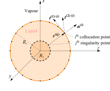
Figure 1: Schematic representation of the collocation and singularity points layout; $\mathbf{n}^{(i)}$, $\mathbf{t}^{(1)(i)}$, and $\mathbf{t}^{(2)(i)}$ represent the unit normal and both the tangential vectors, respectively at the $i$th collocation point.

The flow-field variables are given by a superposition of the Gradlets, thermal Gradlets and sourcelets, formulated in (13-14), as

$$\mathbf{v}^{(i)(Gr)} = \sum_{j=1}^{N^{s}}\frac{1}{8\pi}\mathbf{J}{\left(\mathbf{r}^{(ij)}\right)}\cdot\mathbf{f}^{(j)}+\frac{3\alpha_{0}^{2}c_{p}\mathrm{Kn}^{2}}{4\pi\Pr}\mathbf{K}{\left(\mathbf{r}^{(ij)}\right)}\cdot\mathbf{f}^{(j)}$$ (19a)

$$\mathbf{v}^{(i)(S)} = \sum_{j=1}^{N^{s}}\frac{h^{(j)}}{4\pi}\frac{\mathbf{r}^{\left(ij\right)}}{|\mathbf{r}^{\left(ij\right)}|^{3}}\text{,}$$ (19b)

$$\mathbf{v}^{(i)} = \mathbf{v}^{(i)(Gr)}+\mathbf{v}^{(i)(S)}\text{,}$$ (19c)

$$p^{(i)} = \sum_{j=1}^{N^{s}}\frac{\mathrm{Kn}}{4\pi}\frac{\mathbf{f}^{(j)}\mathbf{\cdot r}^{\left(ij\right)}}{|\mathbf{r}^{\left(ij\right)}|^{3}}\text{,}$$ (19d)

$$\bm{\Pi}^{(i)} = \sum_{j=1}^{N^{s}}\frac{3\mathrm{Kn}}{4\pi}\left(\mathbf{f}^{(j)}\mathbf{\cdot r}^{\left(ij\right)}+2\alpha_{0}\mathrm{Kn}g^{(j)}+2h^{(j)}\right)\mathbf{K}{\left(\mathbf{r}^{(ij)}\right)}\text{,}$$ (19e)

and

$$T^{(i)} = \sum_{j=1}^{N^{s}}\frac{\Pr}{4\pi c_{p}}\frac{g^{(j)}}{|\mathbf{r}^{\left(ij\right)}|}\text{,}$$ (20a)

$$\mathbf{q}^{(i)} = \sum_{j=1}^{N^{s}}\frac{\mathrm{Kn}}{4\pi}\frac{g^{(j)}\mathbf{r}^{\left(ij\right)}}{|\mathbf{r}^{\left(ij\right)}|^{3}}-\frac{3\alpha_{0}c_{p}\mathrm{Kn}^{2}}{4\pi\Pr}\mathbf{K}{\left(\mathbf{r}^{(ij)}\right)}\cdot\mathbf{f}^{(j)}\text{.}$$ (20b)

are fundamental solutions for the CCR equations. Here, $\mathbf{r}^{\left(ij\right)}=\mathbf{r}^{c\left(i\right)}-\mathbf{r}^{s\left(j\right)}$ are the displacement vectors from the $j$th singularity site to the $i$th collocation point.

There are total of $5\times N^{s}$ unknowns in (19-20)—$5$ at each singularity site—which need to be specified via suitable boundary conditions. The $4$ boundary conditions in (16–17) need to be satisfied at every collocation point. Hence, it turns out, one additional boundary condition is required (at each collocation point), we use the following boundary conditions:

$$\mathbf{v}^{(i)(S)}\cdot\mathbf{n}^{(i)} =-\eta_{11}\left(p^{(i)}-p_{sat}^{(i)}+\mathbf{n}^{(i)}\cdot\bm{\Pi}^{(i)}\cdot\mathbf{n}^{(i)}\right)$$

$$\quad+\eta_{12}\left(T^{(i)}-T^{(i)I}+\alpha_{0}\mathbf{n^{(i)}}\cdot\bm{\Pi}^{(i)}\cdot\mathbf{n}^{(i)}\right)\text{,}$$ (21a)

$$\left(\mathbf{v}^{(i)(Gr)}-\mathbf{v}^{\left(i\right)I}\right)\cdot\mathbf{n}^{\left(i\right)} =0\text{,}$$ (21b)

Notably, we have split the boundary condition (16a) into two components (21a) and (21b). Clearly, these two boundary conditions are sufficient for condition (16a) to hold. The boundary conditions for the normal heat-flux (16b) and shear-stress (17) read

$$\mathbf{q}^{(i)}\cdot\mathbf{n}^{(i)} =\eta_{12}\left(p^{(i)}-p_{sat}^{(i)}+\mathbf{n}^{(i)}\cdot\bm{\Pi}^{(i)}\cdot\mathbf{n}^{(i)}\right)$$

$$\quad-\left(\eta_{22}+2\tau_{0}\right)\left(T^{(i)}-T^{(i)I}+\alpha_{0}\mathbf{n^{(i)}}\cdot\bm{\Pi}^{(i)}\cdot\mathbf{n}^{(i)}\right)\text{,}$$ (22a)

$$\mathbf{t}^{(1)\left(i\right)}\cdot\bm{\Pi}^{\left(i\right)}\cdot\mathbf{n}^{\left(i\right)} =-\varsigma\left(\mathbf{v}^{\left(i\right)}\mathbf{-v}^{\left(i\right)I}+\alpha_{0}\mathbf{q}^{\left(i\right)}\right)\cdot\mathbf{t}^{(1)\left(i\right)}\text{,}$$ (22b)

$$\mathbf{t}^{(2)\left(i\right)}\cdot\bm{\Pi}^{\left(i\right)}\cdot\mathbf{n}^{\left(i\right)} =-\varsigma\left(\mathbf{v}^{\left(i\right)}\mathbf{-v}^{\left(i\right)I}+\alpha_{0}\mathbf{q}^{\left(i\right)}\right)\cdot\mathbf{t}^{(2)\left(i\right)}\text{.}$$ (22c)

For convenience, we write the set of equations (21-22) in matrix form :

$$\sum_{j=1}^{N^{s}}\mathbf{\mathscr{L}}^{ij}\mathbf{u}^{\left(j\right)}=\mathbf{b}^{\left(i\right)}\text{,}$$ (23)

where $\mathbf{u}^{\left(j\right)}$ is the vector containing the $5$ degrees of freedom at each singularity point, i.e.,

$$\mathbf{u}^{\left(j\right)}=\left\{g^{\left(j\right)}\text{, }f_{1}^{\left(j\right)}\text{, }f_{2}^{\left(j\right)}\text{, }f_{3}^{\left(j\right)}\text{, }h^{\left(j\right)}\right\}\text{,}$$

Where $\mathscr{L}^{ij}$ is a $5\times 5$ coefficient matrix, and $\mathbf{b}^{\left(i\right)}$ is a $5\times 1$ vector, which can be readily extracted using a symbolic software; we used Mathematica® for this. The inhomogeneous part $\left\{\mathbf{b}^{\left(i\right)}\right\}_{i=1}^{N^{c}}$ contains the properties of the interface, namely, $T^{(i)I}$, $p^{(i)}_{sat}$ and $\mathbf{v}^{\left(i\right)I}$. The $5N^{c}\times 5N^{s}$ linear system (23) is solved for $\left\{\mathbf{u}^{\left(i\right)}\right\}_{i=1}^{N^{s}}$ using an iterative quasi-minimal residual method (Freund & Nachtigal, 1991). Moreover, the normal and the tangent vectors $\left\{\mathbf{n}^{(j)}\text{, }\mathbf{t}^{(1)\left(j\right)}\text{, }\mathbf{t}^{(1)\left(j\right)}\right\}_{j=1}^{N^{c}}$ are obtained using Householder reflection formula for vector orthogonalization (Lopes et al., 2013).

6 Results and discussion

The CCR-MFS described above involves some numerical parameters specifically, how many collocation ($N^{c}$) and singularity ($N^{s}$) points to take, and the location of singularity points outside of the computational domain. These parameters govern the overall efficiency of the numerical scheme, by striking a balance between numerical error and computational time. Throughout this study, we consider an equal number of collocation and singularity points, i.e., $N^{c}=N^{s}$ and take $\gamma\in\left(0,1\right)$ as a geometry-dependent parameter, which governs how far the singularity points are from the boundary. For instance, for the spherical geometry shown in Figure 1, we choose $\gamma=R_{s}/R_{c}$.

In order to validate our code and to establish the numerical accuracy of the CCR-MFS scheme, we validate our results for a case of an evaporating spherical droplet, the analytic solutions to this problems are readily available in (Rana et al., 2018b) for the case of Grad-13 equations. Additionally, in order to establish the accuracy of our models, we consider a slow flow around a sphere (evaporative and non-evaporative) for various values of Knudsen number and compare our solutions with results from kinetic theory.

6.1 Validation and verification of CCR-MSF

6.1.1 Validation case: evaporation from a spherical droplet

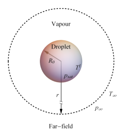
Figure 2: Schematic representation of a liquid droplet surrounded by its own vapour. The equations are made dimensionless with respect to the far-field conditions ($T_{\infty}$, $p_{\infty}$). The temperature and the pressure deviations vanish as $r\rightarrow\infty$.

First, we consider a liquid droplet of fixed radius with a given interface temperature $T^{I}$ and the corresponding saturation pressure $p_{sat}$, immersed in its own vapour; see Figure 2. The far-field conditions are given by $T_{\infty}=0$, $p_{\infty}=0$; that is, we consider the far-field conditions and the droplet radius ($R_{0}$) for non-dimensionalisation. Throughout this article we are not considering dynamics within the droplets, surface tension, etc. see Rana et al. (2019).

Assuming the spherical symmetry of this problem, the analytic solutions for the radial velocity $v_{r}$, heat-flux $q_{r}$, normal stress $\Pi_{rr}$, and the temperature $T$ are obtained from (4-5) as (Rana et al., 2018b)

$$v_{r}=\frac{c_{1}}{r^{2}}\text{, }q_{r}=\frac{c_{2}}{r^{2}}\text{, }\Pi_{rr}=\frac{4\mathrm{Kn}\left(c_{1}+\alpha_{0}c_{2}\right)}{r^{3}}\text{, }T=\frac{\Pr}{c_{p}\mathrm{Kn}}\frac{c_{2}}{r}\text{, and }p=0\text{.}$$ (24)

Here, $r$ is the radial direction; $c_{1}$ and $c_{2}$ are constants of integration. Solutions (24) can also be derived from the fundamental solutions (13a–13c), which are given in Appendix C.

The flow is driven by (i) a unit pressure difference while the temperature of the liquid is equal to the far-field temperature (i.e., $p_{sat}=1$ and $T^{I}=T_{\infty}=0$) or (ii) a unit temperature difference while the saturation pressure in the liquid is same as the far-field pressure (i.e., $p_{sat}=p_{\infty}=0$ and $T^{I}=1$). In both cases, the constants of integration, namely, the mass-flux ($c_{1}$) and heat-flux ($c_{2}$)—per unit area—are obtained from boundary conditions (16) at $r=1$. For Grad-13 (i.e., $\alpha_{0}=2/5$) these are obtained as

$$c_{1}^{p} = 0.220562+\frac{0.0613424+0.0960246\mathrm{Kn}}{0.138548+\mathrm{Kn}(0.716085+\mathrm{Kn})}\text{,}$$ (25a)

$$c_{2}^{p} = c_{1}^{\tau}=-\frac{\mathrm{Kn}(0.108868+0.551404\mathrm{Kn})}{0.138548+\mathrm{Kn}(0.716085+\mathrm{Kn})}\text{,}$$ (25b)

$$c_{2}^{\tau} = \frac{0.152568\mathrm{Kn}+\mathrm{Kn}^{2}(0.924355+1.37851\mathrm{Kn}))}{0.0406847+\mathrm{Kn}(0.348827+\mathrm{Kn}(1.00974+\mathrm{Kn}))}\text{.}$$ (25c)

Here, superscript “$p$” and “$\tau$” denote the pressure-driven case ($p_{sat}=1$ and $T^{l}=T_{\infty}=0$) and temperature-driven case ($p_{sat}=p_{\infty}=0$ and $T^{I}=1$), respectively. The results of these two problems can be combined to evaluate total evaporative mass and heat-flux from the droplet (Rana et al., 2019). Due to the microscopic reversibility of the evaporation and condensation processes the Onsager reciprocity relations hold, which give $\left(c_{2}^{p}=c_{1}^{\tau}\right)$ (Chernyak & Margilevskiy, 1989; Rana et al., 2018b).

The mass and the heat-flux predicted by the CCR–MFS are obtained by integrating $\mathbf{v}^{(Gr)}$ (19a, 19b) and $\mathbf{q}^{(Gr)}$ (20b) over the droplet surface, i.e.,

$$c_{1}^{(MFS)} = \frac{1}{4\pi}\int_{0}^{\pi}\int_{0}^{2\pi}\mathbf{v}^{(Gr)}\cdot\mathbf{n}d\varphi d\theta=\frac{1}{4\pi}\sum_{i=1}^{N^{s}}h^{(i)}\text{,}$$ (26)

$$c_{2}^{(MFS)} = \frac{1}{4\pi}\int_{0}^{\pi}\int_{0}^{2\pi}\mathbf{q}^{(Gr)}\cdot\mathbf{n}d\varphi d\theta=\frac{\mathrm{Kn}}{4\pi}\sum_{i=1}^{N^{s}}g^{(i)}\text{.}$$ (27)

Let us first briefly consider the convergence characteristics of the CCR–MFS. The configuration for the collocation and singularity points is shown in Figure 1. We define errors $\epsilon$ between the numerical prediction of $c_{1}^{p}$, $c_{1}^{T}$, and $c_{2}^{T}$ to the analytical values (25) as

$$\epsilon\left(c_{1}^{p}\right)=c_{1}^{p\left(MFS\right)}-c_{1}^{p}\text{, }\epsilon\left(c_{2}^{\tau}\right)=c_{2}^{\tau\left(MFS\right)}-c_{2}^{\tau}\text{, and }\epsilon\left(c_{1}^{\tau}\right)=c_{1}^{\tau\left(MFS\right)}-c_{1}^{\tau}\text{.}$$ (28)

Figure 3 shows the numerical errors of MFS (with $\alpha_{0}=2/5$) in $c_{1}^{p}$, $c_{2}^{\tau}$ (left) and $c_{1}^{\tau}$ (right) for three different singularity site locations ($\gamma=R_{s}/R_{c}$=0.05, 0.1, 0.25), and various values of the Knudsen number. The result indicates very high accuracy with a moderate number of points ($N^{c}=112$). The best results are obtained when the singularity sites are further away from the collocation nodes, i.e., $\gamma$ is small. However, it leads to poorer conditioning of the equation system (23), which in turn results in larger least-square errors or computational time.

As Lockerby & Collyer (2016), numerical tests were also conducted by increasing the number of collocation points, as well as, by shifting the singularities sites (i.e., breaking the symmetry of the collocation and singularity points); the results were found to be satisfactory. Henceforth, the numerical simulations are performed with $\gamma=0.1$, unless otherwise stated.

Figure 4 shows the variations in the mass and heat-flux coefficients ($c_{1}$ and $c_{2}$) with a range of Knudsen numbers; the numerical parameters are included in the caption. In order to put the CCR models into perspective, we compare our predictions from different theories, namely, NSF ($\alpha_{0}=0$), Grad-13 ($\alpha_{0}=2/5$) and ($\alpha_{0}=3/5$) against the results (symbols) from the linearized Boltzmann equations (LBE) by Takata et al. (1998). The solutions of the NSF equations with classical boundary conditions, i.e., assuming the (linearized) Hertz-Knudsen-Schrage (HKS) law for evaporation (Schrage, 1953) and the continuity of temperature across the interface, are also included (green-thin lines) in Fig. 4 for the comparison. These boundary conditions can be obtained from (16a) by taking $\eta_{12}=0$ and $T=T^{I}$ instead of (16a), which are only valid for $\mathrm{Kn}\rightarrow 0$ (Sone, 2007; Rana et al., 2018b).

For the pressure-driven case (cf., Fig. 4a), mass flux goes from liquid to vapour (i.e., $c_{1}^{p}\geq 0$) and heat flows from vapour to liquid (i.e., $c_{2}^{p}=c_{1}^{\tau}\leq 0$) because the enthalpy of phase change must be supplied to the droplet to keep its temperature constant. All models agree in the limit of $\mathrm{Kn}\rightarrow 0$ for the mass flux; the NSF with temperature jump boundary conditions give better results over classical theories as Knudsen number grows. Interestingly, the NSF with jump boundary conditions predicts a zero mass flux in the free-molecular regime, results contradicting the kinetic theory predictions. On the other hand, the Grad-13 theory gives a non-zero mass flux, but still predicts almost half of the mass flux of the LBE result. By performing an asymptotic expansion, and matching the mass flux as $\mathrm{Kn}\rightarrow\infty$, we find $\alpha_{0}=3/5$, a value extensively used in this study, with this model consequently providing the best agreement with the LBE.

For the temperature-driven case (cf., Fig. 4b), the Fourier’s law with no-jump boundary condition gives heat-flux $c_{2}^{\tau}=15\mathrm{Kn}/4$; while the cross effects, i.e., the heat-flux due to pressure difference or the mass-flux due to temperature difference vanish. We have used this value to normalize the heat-flux computation in Figure 4b. All models, except the no-jump boundary conditions (green-thin lines), match reasonably well with the LBE data, with $\alpha_{0}=3/5$ giving a slight improvement over other models. However, the cross effects ($c_{1}^{\tau}$) are not well captured by CCR theory—which requires resolution of the Knudsen layer—these are beyond the capabilities of the models considered in this paper; see Rana et al. (2018b) for a discussion on .

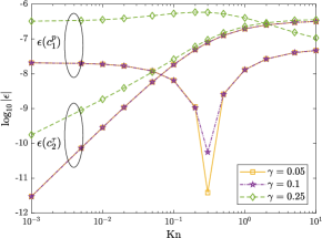
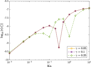
Figure 3: Log-log plot of errors against Knudsen number with three different singularity locations $\gamma=R_{s}/R_{c}=$0.05, 0.1, 0.25 and with $N^{c}=N^{s}=112$: (left) error in $c_{1}^{p}$ and $c_{2}^{\tau}$ and (right) error in $c_{1}^{\tau}$.

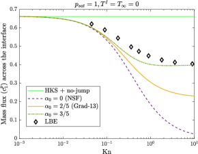
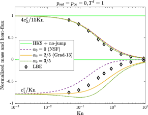
Figure 4: Mass and heat-flux coefficients as a function of the Knudsen number: (a) mass-flux ($c_{1}^{p}$) in pressure-driven case and (b) normalized mass ($c_{1}^{\tau}/\mathrm{Kn}$) and heat-flux ($4c_{2}^{\tau}/15\mathrm{Kn}$) coefficients in the temperature-driven case. The results obtained from MFS with different theories are compared. The symbols denoting the results from Takata et al. (1998) and (green) thin line representing the analytic results from classical boundary conditions. The number of collocation nodes used in each case are $N^{c}=N^{s}$=112 and $\gamma$=0.1.

6.1.2 Slow flow around a rigid sphere

Let us now consider the case of low-speed rarefied gas flow around a rigid ($\vartheta=0$) spherical stationary particle of radius $R_{0}$. The particle is assumed to be isothermal—that is the solid-to-gas conductivity ratio is large—with $T^{I}=0$, i.e., the far-field temperature and the temperature of the particle are same. The net force exerted on the sphere by gas is defined as

$$\mathbf{F}^{(Gr)}=\int_{0}^{\pi}\int_{0}^{2\pi}\left(p^{(Gr)}\mathbf{I}+\mathbf{\Pi}^{(Gr)}\right)\cdot\mathbf{n}d\varphi d\theta=\mathrm{Kn}\sum_{i=1}^{N^{s}}\mathbf{f}^{(i)}\text{.}$$ (29)

The drag force is the projection of the net force (29) onto the stream-wise direction. The Stokes formula for drag force (in the direction of flow) exerted by a spherical particle on the fluid flow has the form Lamb (1945) :

$$F^{S}=-6\pi\mathrm{Kn}u_{\infty}\text{.}$$ (30)

where $u_{\infty}$ is the far-field velocity.

The Stokes formula is only valid for $\mathrm{Kn}\rightarrow 0$, and requires corrections at finite Knudsen number. Figure 5 shows the normalized (with Stokes drag (30)) drag coefficient versus the Knudsen number. As expected, all theories agree in the small Knudsen limit. As the value of Knudsen number increases, the normalized drag decreases due to increasing slip (which is not embedded in Stokes formula). Notably, the normalized drag force reaches a finite value from NSF with velocity-slip boundary conditions as $\mathrm{Kn}\rightarrow\infty$, while the extended theories (CCR) predict a vanishing drag in this limit–an observation tantamount to experimental results. Nevertheless, between Grad-13 ($\alpha_{0}=2/5$) and CCR with phenomenological coefficient $\alpha_{0}=3/5$, the latter gives the best quantitative agreement for values of the Knudsen number beyond unity (i.e. well beyond its apparent limits of applicability).

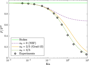
Figure 5: The normalized drag force computed from the CCR-MFS with $\alpha_{0}=0$ (NSF), $\alpha_{0}=2/5$ (Grad-13), and $\alpha_{0}=3/5$ against Knudsen number. The experimental data of Millikan (1923) (fitted by Allen & Raabe (1982)) is plotted (circles) for comparison; the results are normalized with Stokes drag (30).

6.1.3 Slow flow around a spherical liquid droplet

In this section, we consider uniform flow (say, along the z-direction) of a saturated vapour over a spherical liquid droplet with a uniform temperature. The far-field temperature of the surrounding vapour is same as that of the droplet, i.e., $T^{I}=T_{\infty}=0$, $p_{sat}=p_{\infty}=0$, and $\mathbf{v}_{\infty}=-\mathbf{v}^{I}=\left\{0,0,u_{\infty}\right\}$. We further assume that the droplet size remains fixed (quasi-steady state assumption), and deformation of the droplet is negligible, that is, the capillary number is very small.

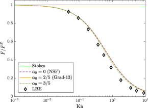
Figure 6: The normalized drag force on a liquid droplet vs Knudsen number. The results computed from the CCR-MSF with $\alpha_{0}=0$ (NSF), $\alpha_{0}=2/5$ (Grad-13), and $\alpha_{0}=3/5$ are compared with LBE data (symbols) of Sone et al. (1994).

Figure 6 shows the normalized drag force on a liquid droplet vs Knudsen number, while allowing phase-change at the interface. This problem has been considered by Sone et al. (1994) from LBE, and is clearly important from an engineering point of view. Due to the motion of the vapour phase, evaporation and condensation take place on the surface of the droplet thereby slightly reducing the drag on the sphere; cf. Figure 5 and 6. Curiously, all theories, except Stokes, give reasonably accurate results. Note that, in this case, the net mass and heat-flux from the droplet are zero with evaporation on the front side of the sphere and condensation on the back.

The problems considered in previous sections typically allow for analytic solutions, which are often not available for various practical problem of interest. In the following sections, we will develop cases of increasing complexity, starting first with the motion over two particles at a finite distance from each other.

6.2 Motion over two solid spheres

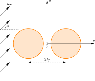
Figure 7: Schematic for the flow around two solid spheres. $2l_{C}$ is the center-to-center distance and $\o$ is the angle between flow direction and the line joining the centers.

Let us consider a flow over two solid spheres with equal radius with both fixed in shape and size . The flow is characterized by the following parameters: radii of the spheres (i.e., the Knudsen number), center-to-center distance $2l_{C}$, and the angle $\o$ between the flow direction and the center-line; see Figure 7.

For an axisymmetric case ($\o=0$), the theoretical results for the drag force (which is equal for both the spheres) calculated by Stimson et al. (1926) read

$$F^{S}=-6\pi\mathrm{Kn}u_{\infty}\beta$$ (31)

where $\beta$ is a correction coefficient which may be written in the form

$$\beta=\frac{4}{3}\sinh{\alpha}\sum_{k=1}^{\infty}\frac{n\left(n+1\right)}{\left(2n-1\right)\left(2n+3\right)}\left(1-\frac{4\sinh^{2}{\left(n+\frac{1}{2}\right)\alpha}-\left(2n+1\right)^{2}\sinh^{2}\alpha}{2\sinh\left(2n+1\right)\alpha+\left(2n+1\right)\sinh 2\alpha}\right).$$ (32)

with $\alpha=\cosh{l_{C}}$.

In Figure 8a, the drag force (normalized with the Stokes’ drag (30) for the single sphere) for an axisymmetric case ($\o=0$) are plotted as a function of center-to-center distance for different values of the Knudsen number. The results from Stimson et al. (1926), which are only valid in the limiting case $\mathrm{Kn}\rightarrow 0$, are included for comparison ($\diamond$);as expected for small value of Knudsen number ($\mathrm{Kn}=10^{-3}$) our results match with Stimson et al. (1926). The experimental results for $\l_{C}=1/2$ obtained by Cheng et al. (1988) (and given by the empirical formula (33)) for $\mathrm{Kn}=10^{-3}$, $10^{-1}$ and $0.5$ are also included ($\mathbf{\times}$) for comparison. For small Knudsen numbers ($\mathrm{Kn}\lesssim 10^{-1}$), all models (NSF, Grad-13, CCR) agree, while at large Knudsen numbers these are markedly different, with the NSF model overpredicting the drag compared to Grad-13 and CCR with $\alpha_{0}=3/5$. The effect of proximity is clearly visible on drag force, which decreases as $l_{C}$ is reduced (i.e., spheres gets closer). Furthermore, in the limit $l_{C}\rightarrow\infty$ the drag approach to the single sphere case (cf., Fig. 5). Also, as with the case of a single sphere (cf., Fig. 5 and 8a), the force monotonically decreases with increases in Knudsen number, for all models.

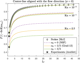
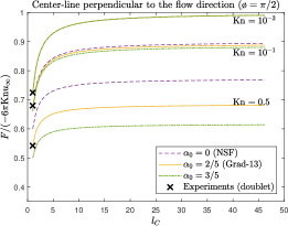
Figure 8: The drag force on two equal spheres vs center-to-center distance: (a) flow direction parallel to their line of centers and (b) flow direction perpendicular to their line of centers. The results computed from the CCR-MSF with $\alpha_{0}=0$ (NSF), $\alpha_{0}=2/5$ (Grad-13), and $\alpha_{0}=3/5$ are compared with Stokes’ solution ($\diamond$) derived by Stimson et al. (1926). The experimental results (denoted by $\mathbf{\times}$) for a doublet ($\l_{C}=1/2$) obtained by Cheng et al. (1988) are included for comparison.

For the nonaxisymmetric case ($\o=\pi/2$), the normalized drag force is plotted in Figure 8b as a function of $l_{C}$, with $\mathrm{Kn}=10^{-3}$, $10^{-1}$ and $0.5$. The experimental results of Cheng et al. (1988) for a doublet ($\l_{C}=1/2$) are denoted by symbols ($\mathbf{\times}$). The overall drag force in the nonaxisymmetric case is higher compared to the axisymmetric case (cf., Figs. 8a and b) and as before, the NSF theory over predicts the drag.

6.2.1 Drag on a doublet

An interesting case arises when one considers $\l_{C}\rightarrow 1/2$, i.e., when both spheres are in contact with one-another—known as a doublet. Cheng et al. (1988) carried out experiments to study the effects of orientation (modulated by an electric electric field) on the measured drag force.

Figure 9 shows a comparison of the different models, computed using CCR-MFS, over a wide range of the Knudsen number. Here, the experimental data for the drag force acting on a doublet is taken from the empirical formula from Cheng et al. (1988), as

$$F=-\frac{4\pi\mathrm{Kn}u_{\infty}}{2^{1/3}}\frac{\phi_{0}}{1+\frac{\mathrm{Kn}}{\phi_{0}}\left[1.142+0.558\exp\left(-0.999\frac{\phi_{0}}{\mathrm{Kn}}\right)\right]}\text{,}$$ (33)

where $\phi_{0}=1.21$ or $\phi_{0}=1.37$ for flow moving in parallel ($\o=0$) or in perpendicular ($\o=\pi/2$) direction to the center line, respectively.

As shown in Figures 9, reassuringly for $\mathrm{Kn}\rightarrow 0$, the results converges to the without-slip solution of the Stokes equation. For larger values of the Knudsen number, the force decreases due to slip, and as $\mathrm{Kn}\rightarrow\infty$, it reaches a finite value for the NSF theory; while from (33) it vanishes. Remarkably, from the results of Grad-13 and CCR models, we find that the force indeed vanishes for large Knudsen numbers. The results obtained from the Grad-13 and CCR models are both in good agreement with the experimental results; a sightly better match at larger Knudsen number is obtained by CCR with $\alpha_{0}=3/5$.

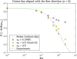
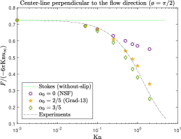
Figure 9: The drag force on a doublet: (a) flow parallel to its line of centers (axisymmetric case) and (b) flow perpendicular to its line of centers (nonaxisymmetric case). The experimental data is taken from the empirical formula (33) obtained in Cheng et al. (1988).

Figures 10 and 11 show the stream-lines and the speed contour for the case $\mathrm{Kn}=0.1$ and $\mathrm{Kn}=0.5$, respectively. The horizontal and vertical axis represent $x$- and $z$-axis, respectively, with flow in $x$-direction. The left hand side of these figures shows the Grad-13 ($\alpha_{0}=2/5$) results for the case $\o=0$, and the right hand side show the results computed from the NSF ($\alpha_{0}=0$) equations. Due to linearity of the equations, the speed contours are symmetric about $x=0$ plane, resulting in equal drag forces on both spheres.

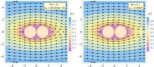
Figure 10: Stream-lines and speed contours from the (left) Grad-13 and (right) NSF equations for Knudsen number 0.1: flow over a doublet with flow direction along the center-line ($\o=0$). Vertical and horizontal axis represents $x$- and $y$-directions. ($N_{c}=N_{s}=650$ and $\gamma=R_{s}/R_{c}=0.1$)

These contours show that, as to be expected, the slip-velocity at the bottom and top surfaces increases with Knudsen number, resulting in reduced drag forces. For $\mathrm{Kn}=0.1$ (Fig. 10), the flow line pattern predicted by the Grad-13 (left) and NSF (right) are very similar. The slip-velocity is maximum near the top and bottom surface, which is virtually the same for NSF and Grad-13 theories, thus giving similar predictions for the drag reduction (cf., Fig. 8). However, for $\mathrm{Kn}=0.5$ (Fig. 11), the Grad-13 theory predicts a larger slip and thus greater drag reduction. The results from CCR with $\alpha_{0}=3/5$ are similar to those obtained from the Grad-13 theory, hence those are not shown here.

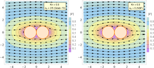
Figure 11: Stream-lines and speed contours from the (left) Grad-13 and (right) NSF equations for Knudsen number 0.5: flow over a doublet with flow direction along the center-line ($\o=0$). Vertical and horizontal axis represents $x$- and $y$-directions. ($N_{c}=N_{s}=650$ and $\gamma=R_{s}/R_{c}=0.1$)

In Figures 12 and 13, we again show the stream-lines and speed contours predicted by both theories at $\mathrm{Kn}=0.1$ and $\mathrm{Kn}=0.5$, respectively, for the case when flow (in $z$-direction) is in perpendicular direction to the center-line, i.e., $\o=\pi/2$. Unlike the previous case, this is a truly 3D setup, where no symmetry exist in the azimuthal direction—with the MFS it is remarkably simple to solve this fully 3D flow. The slip velocity increases with increasing the Knudsen number thus reducing the drag coefficient.

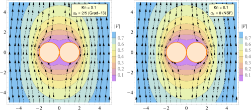
Figure 12: Stream-lines and speed contours from the (left) Grad-13 and (right) NSF equations for Knudsen number 0.1: flow over a doublet with flow direction perpendicular to the center-line ($\o=\pi/2$). Vertical and horizontal axis represents $x$- and $y$-directions. ($N_{c}=N_{s}=650$ and $\gamma=R_{s}/R_{c}=0.1$)

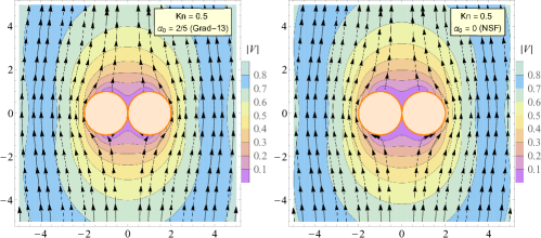
Figure 13: Stream-lines and Mach contours from the (left) Grad-13 and (right) NSF equations for Knudsen number 0.5: flow over a non-evaporative ($\vartheta=0$) doublet with flow direction perpendicular to the center-line ($\o=\pi/2$). Vertical and horizontal axis represents $x$- and $y$-directions. ($N_{c}=N_{s}=650$ and $\gamma=R_{s}/R_{c}=0.1$)

6.3 Interaction of two evaporating droplets

The evaporation dynamics of two interacting droplets suspended in vapour will be investigated here; a problem relevant for dense spray applications. We consider two droplets placed is a saturated vapour with center-to-center distance $2l_{C}$. Again, we consider the shape, size and the surface temperature of the droplet fixed.

As before, we consider two cases, i.e., (i) evaporation is driven by temperature difference (i.e., $p_{sat}=p_{\infty}=0$ and $T^{I}=1$) and (ii) evaporation due to pressure difference ($p_{sat}=1$ and $T^{I}=T_{\infty}=0$). The distance between two droplets and the Knudsen number are varied in order to investigate the proximity and rarefaction effects. The results from three models are compared NSF, Grad-13 and CCR with $\alpha_{0}=3/5$.

Temperature driven case: In Figures 14, we show the mass-flux and the heat-flux per unit area as a function of Knudsen number for the temperature-driven case. The mass-flux reduces monotonically with the Knudsen number while the NSF theory predicts a higher mass-flux than CCR. Figures 14a and 14b illustrate the mass-flux with center-to-center distance $2l_{C}=0.001$ (i.e., when the droplets are next to each other) and $2l_{C}=10$ (i.e., at a distance where proximity effects are negligible), respectively. The corresponding heat-flux is shown in Figures 14c and 14d.

When droplets are next to each other a shielding effect is observed, and, as a result, the mass-flux reduces (cf. Figures 14a and b). At $\mathrm{Kn}=0.05$, all three models predict about $29\%$ reduction in the mass-flux as compared to a single droplet (i.e., $l_{C}\rightarrow\infty$). The reduction in the mass-flux decreases with increase in Knudsen number. For $\mathrm{Kn}=1$, NSF, Grad-13 and CCR with $\alpha_{0}=3/5$ predicts about $9\%$ , $13\%$ and $12\%$ reduction in mass-flux, respectively.

The mass-fluxes computed from the MFS (symbols) for center-to-center distance $10$ are shown in Figure 14b; the analytic results from a single droplet are also plotted (continuous lines) for comparison. As expected, as the droplets are moved further apart, the results converges to the single droplet cases; the mass-flux is within $5\%$ (for $\mathrm{Kn}=0.05$) and $1\%$ (for $\mathrm{Kn}=1$) for the single droplet case.

Similarly, the proximity effects on the heat-flux are visible in Figures 14c and 14d, for $2l_{C}=0.001$ and $2l_{C}=10$, respectively. Again, the heat flux reduces as $l_{C}\rightarrow 1/2$, and as the value for the Knudsen number increases the proximity effects diminish. The percentage difference in the heat-flux from the single droplet cases varies from about $29\%$ to $12\%$ for $2l_{C}=1.001$ and from about $4\%$ to $1\%$ for $2l_{C}=10$, as the value of Knudsen number varies from $0.05$ to 1.

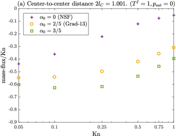
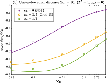
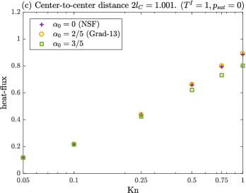
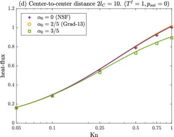
Figure 14: Two interacting droplets for the temperature driven case ($T^{I}=1,p_{sat}=0$): Profiles of the (a) mass-flux with center-to-center distance $2l_{C}=0.001$, (b) mass-flux with $2l_{C}=10$ (c) heat-flux with $2l_{C}=0.001$ and (d) heat-flux with $2l_{C}=10$ as functions of the Knudsen number for NSF, Grad-13 and CCR with $\alpha_{0}=3/5$. Symbols denote MFS solutions and curves represent analytic solution from a single droplet.

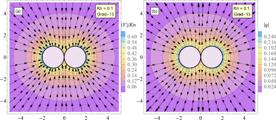
Figure 15: Two droplets placed adjacent to each other ($2l_{c}=1.001$) for the temperature driven case ($T^{I}=1,p_{sat}=0$): (a) streamlines and speed contours (b) heat-flux lines and magnitude, obtained from the Grad-13 MFS solution. Vertical and horizontal axis represents $x$- and $y$-directions. ($N_{c}=N_{s}=650$ and $\gamma=R_{s}/R_{c}=0.1$).

The vaporization dynamics of a pair of droplets placed adjacent to each other is markedly different from the single droplet counterpart. In Figure 15, (a) the stream lines superimposed on the velocity magnitude contours, and (b) the heat-flux lines and the magnitude contours are shown. The heat goes out of the hot droplets due to negative temperature gradients while the condensation occurs in order to compensate for the heat loss. Figure 15 shows that the mass-flux and the heat-flux at the confined region between droplets are sufficiently lower than outer regions. In this region, the vapour temperature is relatively high, thus a smaller temperature jump which leads to a reduced mass-flux and heat-flux.

Pressure driven case: In Figure 16, we show the (a) mass-flux with center-to-center distance $2l_{C}=0.001$, (b) mass-flux with $2l_{C}=10$ (c) heat-flux with $2l_{C}=0.001$ and (d) heat-flux with $2l_{C}=10$ as functions of the Knudsen number for the pressure driven case. Again, in order to gain insights into the proximity effects, the numerical solution obtained via MFS (symbols) and the analytic results from a single droplet case (continuous lines) are compared in Figure 16. The this case, the mass-flux is slightly reduced ($\lesssim 3\%$ for $2l_{C}=0.001$ and $\lesssim 0.06\%$ for $2l_{C}=10$) between the range ($0.05\leq\mathrm{Kn}\leq 1$). On the other hand, the proximity effects on the heat flux are observed to be significant. For $2l_{C}=0.001$, the magnitude of the heat-flux is reduced about $29.3\%$ for NSF ($28.7\%$ for Grad-13 and CCR) at $\mathrm{Kn}=0.05$ and about $10\%$ for NSF ($\leq 15\%$ for Grad-13 and CCR) at $\mathrm{Kn}=1$. For $2l_{C}=0.001$, all models give less than $4\%$ reduction in the heat flux, for all range of the Knudsen number considered.

Another interesting point to be noted from Figures 16(c), (d) is that the heat-flux predicted by the NSF equations is significantly lower in magnitude compared to the CCR and Grad-13 models, especially in the transition regime ($\mathrm{Kn}\geq 0.1$). Within this regime, the heat-flux is not only driven by the temperature gradient (i.e., Fourier’s law) but also due to the pressure gradient; this second-order effect can easily be understood from the constitutive relations (5) and the momentum balance equation (4), which give

$$\mathbf{q}=-\frac{c_{p}\mathrm{Kn}}{\Pr}\left(\nabla T-\alpha_{0}\nabla p\right).$$ (34)

Here, the second term on the right-hand-side is the non-Fourier contribution to the heat flux due to pressure gradient (Rana et al., 2018a). In Figure 17, we show two different contributions to the scaled normal heat-flux ($\mathbf{q}\cdot\mathbf{n}/\mathrm{Kn}$) along the surface of the droplet (in $x$-$z$ plane) for the pressure-driven case with $\mathrm{Kn}=0.1$. As predicted from the Grad-13 theory, the heat-flux owing to pressure gradient (non-Fourier) and heat-flux due to temperature gradient (Fourier) have opposing effects, and consequently the net heat-flux is reduced in the second-order theories.

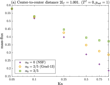
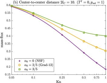
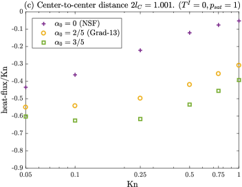
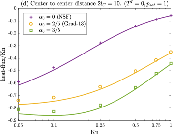
Figure 16: Two interacting droplets for the pressure driven case ($T^{I}=0,p_{sat}=1$): Profiles of the (a) mass-flux with center-to-center distance $2l_{C}=0.001$, (b) mass-flux with $2l_{C}=10$ (c) heat-flux with $2l_{C}=0.001$ and (d) heat-flux with $2l_{C}=10$ as functions of the Knudsen number for NSF, Grad-13 and CCR with $\alpha_{0}=3/5$. Symbols denote MFS solutions and curves represent analytic solution from a single droplet.

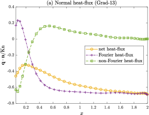
Figure 17: Two interacting droplets for the pressure driven case ($T^{I}=0,p_{sat}=1$): Fourier and non-Fourier contributions to the normal heat-flux ($\mathbf{q}\cdot\mathbf{n}/\mathrm{Kn}$) given by the Grad-13 theory plotted along the top surface of the droplet in $x$-$z$ plane.

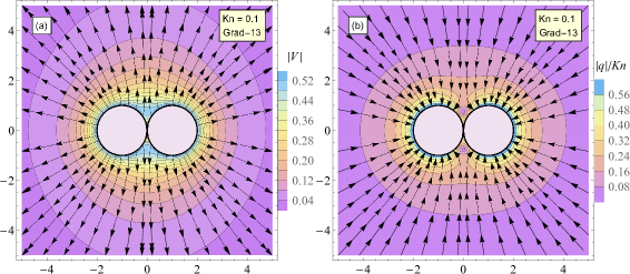
Figure 18: Two droplets placed next to each other ($2l_{c}=1.001$) for the pressure driven case ($T^{I}=0,p_{sat}=1$): (a) stream lines and speed contours (b) heat-flux lines and magnitude, obtained from the Grad-13 MFS solution. Vertical and horizontal axis represents $x$- and $y$-directions. ($N_{c}=N_{s}=650$ and $\gamma=R_{s}/R_{c}=0.1$).

In Figure 18, we again show the streamlines and the velocity magnitude contours (a), and the heat-flux lines and the magnitude contours (b) for the pressure driven case. In this case, evaporation occurs due to a negative pressure gradient and the heat flows inwards. The mass-flux and the heat-flux at the confined region between droplets are reduced due to a high vapour pressure.

The high-pressure region created between two droplets pushes them away from each other. The net drag force (in the $x$ direction) acting on each droplet is plotted in Figure 19 as a function $\mathrm{Kn}$. The results for various values of center-to-center distance shown in Figure 19 are computed from the Grad-13 model; the drag force predicted by the NSF model is within $10\%$ and not shown. The force decreases exponentially as droplets become further apart, i.e., as $l_{C}$ increases. Interestingly, the drag force attains a minimum value at a certain Knudsen number, which depends on how far the droplets are from each other. As $\mathrm{Kn}\rightarrow\infty$, the drag force vanishes.

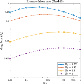
Figure 19: The drag force acting on the droplets vs Knudsen numbers for various values of the separation distance as predicted by the Grad-13 theory for the pressure driven case.

6.4 Evaporation of a deformed droplet

In this section, we shall study evaporation/condensation from a deformed droplet with fixed shape and sized, in order to gain some initial insight into evaporation occurring during oscillatory and/or deformed droplet events—leaving the step to unsteady flow as a focus for future work. The effects of heat conduction and the flow inside the droplet are not considered. The parametric equation for the droplet surface in the second harmonic mode is given by (e.g., see Sprittles & Shikhmurzaev (2012))

$$\vec{X}=\eta_{0}\left[1+\frac{\eta}{2}\left(3\cos^{2}\phi-1\right)\right]\left\{\sin\phi\cos\theta,\sin\phi\sin\theta,\cos\phi\right\}$$ (35)

where $\phi\in[0,\pi]$ and $\theta\in[0,2\pi]$ and $\eta$ is the shape factor. The volume of the droplet is

$$V=\eta_{0}\frac{4\pi}{3}\left(\frac{35+21\eta^{2}+2\eta^{3}}{35}\right)^{1/3}\text{.}$$ (36)

Therefore, in order to have the volume $V$ equal to a spherical droplet of radius $1$, the normalizing factor $\eta_{0}$ is given by

$$\eta_{0}=\left(\frac{35}{35+21\eta^{2}+2\eta^{3}}\right)^{1/3}\text{.}$$ (37)

The droplet shapes with different values of shape parameter $\eta=0,0.5$ and $1$ are depicted in Figure 20; the corresponding (non-dimensional) surface area of the droplets are $4\pi,4\pi\times 1.078$ and $4\pi\times 1.192$, respectively.

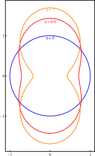
Figure 20: Droplet shapes given by second spherical harmonics with shape parameter $\eta=0,0.5,1$ and the normalizing factor $\eta_{0}=35^{1/3}/(35+21\eta^{2}+2\eta^{3})^{1/3}$ ensuring that the droplet has fixed volume.

We shall again consider two cases: (i) flow due to a unit pressure difference while the temperature of the liquid is equal to the far-field temperature (i.e., $p_{sat}-p_{\infty}=1$ and $T^{l}-T_{\infty}=0$) and (ii) flow due to a unit temperature difference while the saturation pressure in the liquid is same as the far-field pressure (i.e., $p_{sat}-p_{\infty}=0$ and $T^{l}-T_{\infty}=1$).

Pressure-driven case: In Figures 21(a), (b) and (c), we show the mass-flux per unit area as a function of $\mathrm{Kn}$ computed using NSF, Grad-13 and $\alpha_{0}=3/5$ models, respectively for the shape parameter $\eta=0,0.5,1$. Here, the numerical results from MFS are denoted by symbols and the analytic results for the spherical droplet ($\eta=0$) are represented by the solid line. For small deformity ( $\eta=0,0.5$) mass-flux is nearly same, however when the droplet is more deformed ($\eta=1$) the mass-flux is reduced. The percentage reduction in the mass-flux (compared to a spherical droplet) is about $11\%$ for $\mathrm{Kn}=0.05$ and about $21\%$ for $\mathrm{Kn}=1$. Similar to the case of two droplets placed next to each other, considered in the previous section, the reduction in the mass-flux is due to formation of a high pressure in the high curvature (for $\eta=1$) cusp region near $z=0$, which is not present at smaller $\eta$.

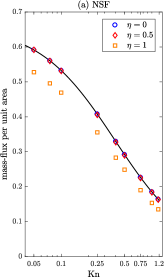
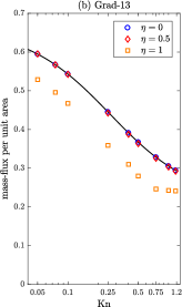
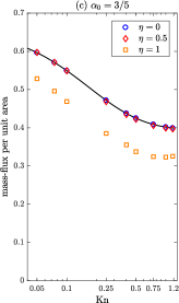
Figure 21: Pressure-driven case ($p_{sat}-p_{\infty}=1$, $T^{l}-T_{\infty}=0$): mass flux per unit area vs Knudsen number with $\eta=0,0.5,1$. (a) NSF, (b) Grad-13, and (c) $\alpha_{0}=3/5$.

The symbols denote the MSF solutions and the solid lines represent analytic results for a spherical droplet.

Similarly, in Figures 22(a), (b) and (c) we plot the heat-flux per unit area as a function of $\mathrm{Kn}$ for the same shape parameters. Note that the heat-flux due to pressure difference is a first order quantity in terms of $\mathrm{Kn}$ (that is it vanishes as $\mathrm{Kn}\rightarrow 0$), hence in these figures we have scaled the heat-flux with inverse $\mathrm{Kn}$. Again, the magnitude heat flux magnitude reduces as $\eta\rightarrow 1$. The reduction in the heat-flux is about 13% Furthermore, the Grad-13 and CCR theories predict a larger heat-flux compared to the NSF results due to non-Fourier heat-flux contribution (34).

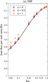
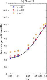
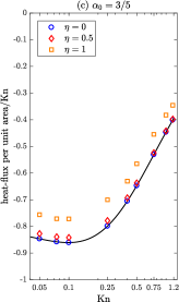
Figure 22: Pressure driven case ($p_{sat}-p_{\infty}=1$, $T^{l}-T_{\infty}=0$): heat flux per unit area/$\mathrm{Kn}$ vs Knudsen number with $\eta=0,0.5,1$. (a) NSF, (b) Grad-13, and (c) $\alpha_{0}=3/5$.

The symbols denote the MSF solutions and the solid lines represent analytic results for a spherical droplet.

Temperature driven case: In Figure 23, we present the heat-flux per unit area for the temperature driven case for different shape factors (see legend in the figures) for NSF (in sub Figure (a)), Grad-13 (sub Figure (b)) and CCR with $\alpha_{0}=3/5$ (sub Figure (c)). Note that, due to the Onsager reciprocity relations (Chernyak & Margilevskiy, 1989), the mass-flux for the temperature driven case is same as the heat-flux for the pressure driven case (Figure 22) hence it is not shown. Evidently, form Figures 23, the magnitude of the heat-flux reduces with the deformation, i.e., as $\eta\rightarrow 1$. For NSF (Figure 23(a)); the reduction is about 3% for $\eta=0.5$ and about 12% for $\eta=1$.

Curvature dependence of the saturation pressure: Throughout this article, we have taken $T^{I}$ and $p_{sat}$ as independent parameters. However, in general, the Clausius-Clapeyron-Kelvin formula provides a relation between the saturation pressure and the temperature at the interface (linearized and dimensionless) (McElroy, 1979; Bond & Struchtrup, 2004):

$$p_{sat}\left(T^{I}\right)=p_{sat}^{p}\left(T^{I}\right)\underline{\exp\left(2\gamma\kappa\right)}\text{.}$$ (38)

Here, $\gamma$ is the dimensionless surface tension ($\gamma=\hat{\gamma}/\hat{\rho}_{l}\hat{\ell}\hat{R}\hat{T}_{0}$), $\kappa$ is the dimensionless curvature ($\kappa=\hat{\kappa}\hat{\ell}$) and $p_{sat}^{p}\left(T^{I}\right)=H_{0}T^{I}$ is the saturation pressure for a planar surface with $H_{0}$ ($=\hat{H}_{0}/\hat{R}\hat{T}_{0}$) being the dimensionless heat of evaporation.

Thus far, the modelling assumption has been that $H_{0}$ (and $\gamma$) can be independently chosen to give a desired value of the saturation pressure. Notably, for the noble gases (vapour/liquid) the Kelvin correction term (underlined) in equation (38) are often small, unless the radius of curvature $\hat{\kappa}$ is in nano-meters. For example, for Argon, if we choose $\hat{T}_{0}=103\,\mathrm{K}$, $\hat{p}_{0}=p^{p}_{sat}\left(\hat{T}_{0}\right)=0.4\,\mathrm{MPa}$, $\hat{\rho}_{l}=1294.6\,\mathrm{kg/m^{3}}$, $\hat{\gamma}=8.75\,\mathrm{mN/m}$ [a case considered in (Rana et al., 2019)], the Kelvin correction term gives $\exp\left(0.6305/a\right)$, where $a$ (in $\mathrm{nm}$) is the inverse of local curvature $\hat{\kappa}$. Therefore, for a drop of size greater than $10\,\mathrm{nm}$, the effect of the Kelvin correction term will be less then $6.1\%$.

In order to compare our results with existing literature, in §7 we shall use the dimensionless heat of evaporation $H_{0}$ as an independent parameter.

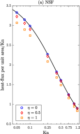
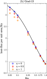
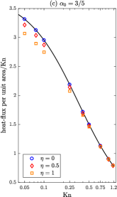
Figure 23: Temperature driven case ($p_{sat}-p_{\infty}=0$, $T^{l}-T_{\infty}=1$): heat flux per unit area/$\mathrm{Kn}$ vs Knudsen number with $\eta=0,0.5,1$. (left) NSF, (middle) Grad-13, and (right) $\alpha_{0}=3/5$.

The symbols denote the MSF solutions and the solid lines represent analytic results for a spherical droplet.

7 Inverted temperature profile and Knudsen layer

A notorious deficiency of NSF and CCR theories is their inability to capture the Knudsen layer—a kinetic boundary layer extending within a few mean free path into the domain (Sone, 2007; Struchtrup & Torrilhon, 2008; Torrilhon, 2016). We have seen in previous sections that the CCR model is able to predict global flow features, such as net mass flux, heat flux and drag; however, it may fail to describe finer flow features especially those in which Knudsen layer and other rarefaction effects are dominant. In this section, we shall consider such a case.

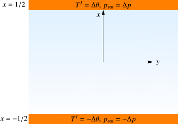
Figure 24: Schematic for heat and mass transfer between two liquid layers.

Let us consider heat and mass transfer between two liquid layers located at locations $x=\pm 1/2$, see Figure 24. We prescribe the dimensionless temperatures and saturation pressures of the liquid layers as $T^{I}\left(\pm 1/2\right)=\pm\Delta\theta$ and $p_{sat}\left(\pm 1/2\right)=\pm\Delta p$. For a planar surface, $\hat{\kappa}=0$, and thus $\Delta p=\Delta\theta H_{0}$.

After some calculation, the analytic solution of the linear problems (4) and (5) assumes the form

$$v_{x} = c_{1}\text{, }q_{x}=c_{2}\text{, }T=-\frac{\Pr c_{2}}{c_{p}\mathrm{Kn}}x\text{,}$$ (39a)

$$p = \sigma_{xx}=0\text{,}$$ (39b)

where $c_{1}$ and $c_{2}$ are integration constants, which need to be evaluated using boundary conditions. Solving (16) for $c_{1}$ and $c_{2}$ gives

$$c_{1} = \sqrt{\frac{2}{\pi}}\left(\frac{(0.306763+1.62499\mathrm{Kn})H_{0}-0.741358\mathrm{Kn}}{0.370583+1.77245\mathrm{Kn}}\right)\Delta\theta\text{,}$$ (40a)

$$c_{2} = \frac{5\mathrm{Kn}}{2\mathrm{Pr}}\left(\frac{0.741165-0.157738H_{0}}{0.370583+1.77245\mathrm{Kn}}\right)\Delta\theta\text{.}$$ (40b)

Note that, for this problem, the CCR reduces to NSF constitutive relations.

Interestingly, as can be seen from inspection of (40b), the conductive heat flux $q_{x}$ switches sign for $H_{0}\geq 4.7$, which leads to an inverted temperature profile in the vapour—this is qualitatively consistent with kinetic theory (Pao, 1971) and MD simulations (Frezzotti et al., 2003). Notably, the NSF equations with classical boundary conditions, i.e., with no-temperature jump boundary conditions along with the Hertz-Knudsen-Schrage can not describe the inverted temperature phenomenon.

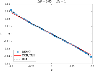
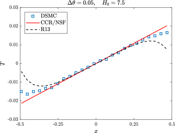
Figure 25: Temperature profiles as functions of location $x$ for $\left(\Delta\theta=0.05\text{, }H_{0}=1\right)$ (left) and $\left(\Delta\theta=0.05\text{, }H_{0}=7.5\right)$ (right) for $\mathrm{Kn}=0.078$. The figure on right demonstrates the inverted temperature profile.

Figures 25(i) and (ii) show the temperature curves as functions of $x$ for $\Delta\theta=0.05\text{, }H_{0}=1\left(<4.7\right)$ and $\Delta\theta=0.05\text{, }H_{0}=7.5\left(>4.7\right)$, respectively, for $\mathrm{Kn}=0.078$. These flow parameters are chosen so that our results can be compared with those obtained from the DSMC and R13 theories given in (Beckmann et al., 2018). Comparing both cases, when $H_{0}$ is smaller than the critical heat of evaporation (case 1) the temperature profile shows a large jump at both boundaries with higher temperature on the lower boundary. In this case, the mass and heat fluxes are both positive (i.e., from lower boundary to upper) and as expected, the temperature is higher at the lower boundary. On the other hand, in case 2, $H_{0}$ is larger then the critical heat of evaporation and the temperature profile is inverted. For this case the heat flows from the hot side (where condensation occurs) towards the cold side (where evaporation occurs). The results from the DSMC are denoted by symbols.

Evidently, the CCR theory qualitatively explains the intriguing inverted temperature phenomenon. However, the CCR model does not provide detail of the temperature profiles near to the boundaries; the region which is dominated by the Knudsen layer. The R13 theory provides improvement in predicting the temperature profile at this value of the Knudsen number because, as is well known, it can capture some basic features of the Knudsen layer.

8 Conclusion and future directions

The present article studies liquid vapour phase-transition processes in which $\mathrm{Kn}\lesssim 1$, i.e., down to sub-micron scales. In particular, we derive a set of fundamental solutions for the CCR system which allows for three-dimensional multiphase micro flows at remarkably low computational cost—the fundamental solutions to the linearised NSF and Grad-13 equations are obtained as a special case. A set of thermodynamically consistent liquid-vapour interface conditions for the linearised CCR system are derived within the framework of irreversible thermodynamics.

Different macroscopic models were applied to solve the motion of a sphere is a gas and compared the results with theoretical and experimental results from the literature. We observed that the results for the drag force obtained from the Grad-13 and CCR model are both in good agreement with the experimental results; a slightly better match at larger Knudsen number is obtained by taking $\alpha_{0}=3/5$.

The motion of two spherical particles was investigated and compared to the classical Stokes solutions and experimental results. The drag force reduces as the Knudsen number increases, mainly due to velocity slip at the surface. The effect of proximity is investigated on the drag force, which decreases as particles gets closer. For a doublet, contrary to the experimental observations, the Stokes and NSF equations predict a non-zero drag while the Grad-13 and CCR with coupling coefficient $\alpha_{0}=3/5$ provide excellent match with the experimental data. Proximity effects on mass and heat transfer coefficients of two interacting droplets were investigated over a range of Knudsen numbers. Two far-field conditions were examined: (i) Pressure driven where $p_{sat}-p_{\infty}=1$, $T^{l}-T_{\infty}=0$, and (ii) Temperature driven where $p_{sat}-p_{\infty}=0$, $T^{l}-T_{\infty}=1$. However, due linearity of the governing equations and the boundary conditions involved, these two cases can be combined to give results for a general case. For the pressure-driven case a slight reduction ($\lesssim 3\%$) in the mass-flux was observed when the droplets are placed next to each other. On the other hand, the heat-flux was significantly reduced ($\sim 30\%$). For the temperature driven case, the situation is reversed, where a significant reduction in the mass-flux was observed due to shielding effects. We also considered the case of a single deformed droplet and studied the effects of deformity on the mass and heat transfer characteristics over a range of the Knudsen number.

Motivated by these findings, future work could be to extend this work to study phase transition process in polyatomic fluids and binary mixtures.

Extension of the current work to unsteady flows and coupling to liquid dynamics (Rana et al., 2019; Chubynsky et al., 2020) can be considered in future—the liquid phase can be modelled as an incompressible fluid (Stokeset/Oseenlet and heatlet) and the vapor phase modelled via CCR model. However, it will require solving the moving boundary problem efficiently within the MFS framework (Jiang et al., 2014). Another line of inquiry would be to implement these fundamental solutions via boundary integral methods which offer more flexibility and robustness as compared to the MFS. A prominent deficiency of NSF and CCR model is their inability to capture the Knudsen layer—a kinetic boundary layer extending a few mean free paths into the domain. Future work can also include finding fundamental solutions to the linearised R26-equations in order to incorporate Knudsen layers. The cornerstone of this work is the linearity of the differential operators involved, which allow us to obtain Green’s functions and formulate the MFS. As such, the method developed here can not be directly applied to non-linear problems. In another context, MFS has been applied to some non-linear problems using appropriate fixed point iterative schemes (Fan et al., 2009). It would be interesting to attempt a similar approach for solution of the nonlinear CCR model and/or nonlinear boundary conditions.

9 Acknowledgments

This work has been partially supported via Scheme for Promotion of Academic and Research Collaboration (SPARC) grant (IDN_SKI 444) funded by the Ministry of Human Resources Development (MHRD), India and EPSRC Grants No. EP/N016602/1, EP/P031684/1, EP/S029966/1. The authors are grateful to Dr. Juan Padrino from the University of Warwick for many fruitful discussions on Green’s functions.

10 Declaration of Interests

The authors report no conflict of interest.

Appendix A Derivation of the Green’s functions for the Sourcelet

The Fourier transformation of the energy conservation law (11₃) and the heat flux constitutive relation (5₂) gives

$$\mathbf{k}\cdot\mathbf{\tilde{q}}=0\text{, and \quad}\mathbf{\tilde{q}}=i\frac{c_{p}Kn}{\Pr}\mathbf{k}\tilde{\Theta}\text{,}$$ (41)

where we have defined $\Theta=T-\alpha_{0}p$ and its Fourier transformation $\mathcal{F}\left[\Theta\left(\mathbf{r}\right)\right]=\tilde{\Theta}\left(\mathbf{k}\right)$. Clearly, the inverse Fourier transformation of (41) leads to

$$\mathbf{q=0}\text{, and \quad}\Theta=0\text{.}$$ (42)

Similarly, taking a Fourier transformation of (11_1,2), one obtains

$$\mathbf{k}\cdot\mathbf{\tilde{v}}=ih\text{, and \quad}\tilde{p}\mathbf{k}+\tilde{\Pi}\cdot\mathbf{k}=\mathbf{0}\text{,}$$ (43)

where from (5₁)

$$\tilde{\bm{\Pi}}=i\mathrm{Kn}\left(\mathbf{\tilde{v}k}+\mathbf{k\tilde{v}}-\frac{2}{3}\left(\mathbf{k}\cdot\mathbf{\tilde{v}}\right)\mathbf{I}\right)\text{.}$$ (44)

Equations (43 and 44) give

$$\tilde{v}=ih\frac{\mathbf{k}}{|k|^{2}},\text{\quad}\tilde{\bm{\Pi}}=-2\mathrm{Kn}h\left(\frac{\mathbf{kk}}{|k|^{2}}-\frac{1}{3}\mathbf{I}\right)\text{, \quad}\tilde{p}=\frac{4}{3}\mathrm{Kn}h\text{.}$$ (45)

Finally, taking the inverse Fourier transformation of (45) yields

$$\mathbf{v} = ih\mathcal{F}^{-1}\left[\frac{\mathbf{k}}{|k|^{2}}\right]=\frac{h}{4\pi}\frac{\mathbf{r}}{|r|^{3}},\quad p=0\text{, and}$$

$$\mathbf{\bm{\Pi}} = -2\mathrm{Kn}h\mathcal{F}^{-1}\left[\frac{\mathbf{kk}}{|k|^{2}}-\frac{1}{3}\mathbf{I}\right]=\frac{3\mathrm{Kn}h}{2\pi}\frac{1}{|r|^{5}}\left[\mathbf{rr}-\frac{1}{3}|r|^{2}\mathbf{I}\right]\text{.}$$

Here, we have used the following inverse Fourier transformation identities:

$$\mathcal{F}^{-1}\left[\frac{\mathbf{k}}{|k|^{2}}\right]=-\frac{i}{4\pi}\frac{\mathbf{r}}{|r|^{3}}\text{, and }\mathcal{F}^{-1}\left[\frac{\mathbf{kk}}{|k|^{2}}\right]=-\frac{3}{4\pi}\left[\frac{\mathbf{rr}}{|r|^{5}}-\frac{1}{3|r|^{3}}\mathbf{I}\right]\text{.}$$ (46)

Appendix B Phenomenological coefficients in the boundary conditions

The numerical coefficients appearing in the phenomenological boundary conditions are based on Sone (2007), where these were obtained by an asymptotic expansion of the linearized Boltzmann equation for $\mathrm{Kn\rightarrow 0}$. The coefficients $\eta_{ij}$ appearing in equations (18) can be directly compared to Sone (2007), as

$$\eta_{11} = -\frac{4\sqrt{\pi}d_{1}}{4C_{4}^{\ast}d_{1}+5\text{$\gamma$}_{2}d_{4}^{\ast}}\text{, \quad}\eta_{12}=\frac{5\sqrt{\pi}\text{$\gamma$}_{2}d_{4}^{\ast}}{4C_{4}^{\ast}d_{1}+5\text{$\gamma$}_{2}d_{4}^{\ast 2}}$$ (47)

$$\eta_{12} = -\frac{25\sqrt{\pi}\text{$\gamma$}_{2}^{2}d_{4}^{\ast 2}}{16C_{4}^{\ast}d_{1}^{2}+20\text{$\gamma$}_{2}d_{1}d_{4}^{\ast 2}}\text{, and \quad}\tau_{0}=\frac{5\sqrt{\pi}\text{$\gamma$}_{2}}{8d_{1}}$$ (48)

Here, the values of $\gamma$₁, $\gamma$₂, $d_{1}$, $d_{4}^{\ast}$ and $C_{4}^{\ast}$ for a hard-sphere gas (HS) and for the BGK model (BGK) are given in Table 1:

	$\gamma$1	$\gamma$2	$d_{1}$	$d_{4}^{\ast}$	$C_{4}^{\ast}$
HS	$1.27004$	$1.9223$	$2.4001$	$-0.4557$	$-2.1412$
BGK	$1$	$1$	$1.3027$	$-0.4467$	$-2.1320$

Table 1: The values of $\gamma_{1}$, $\gamma_{2}$, $d_{1}$, $d_{4}^{\ast}$ and $C_{4}^{\ast}$ for a hard-sphere gas (HS) and for the BGK model (BGK). Data taken from Sone (2007).

Appendix C Analytic solutions obtained from fundamental solutions

The analytic solutions (24) for an evaporating spherical droplet can also be obtained from the fundamental solutions (13a–13c). Due to the spherical symmetry let us place one singular mass source of strength $h$ and a heat source of strength $g$ at the origin. Let $\mathbf{r}=r\left\{\cos\phi\sin\theta,\sin\phi\sin\theta,\cos\theta\right\}$ be an arbitrary point outside the droplet ($r\geq 1$). From (3.7–3.8) we get

$$\mathbf{v}\left(\mathbf{r}\right)\cdot\mathbf{n}=\frac{h}{4\pi r^{2}}\text{, }p\left(\mathbf{r}\right)=0\text{, }\mathbf{n}\cdot\sigma\left(\mathbf{r}\right)\cdot\mathbf{n=}\frac{\mathrm{Kn}\left(h+\text{$\alpha_{0}$}g\mathrm{Kn}\right)}{\pi r^{3}}$$ (49)

and

$$T\left(\mathbf{r}\right)=\frac{\text{$\Pr$}}{\text{$c_{p}$}}\frac{g}{4\pi r}\text{, }\mathbf{q}\left(\mathbf{r}\right)\cdot\mathbf{n}=\frac{\mathrm{Kn}g}{4\pi r^{2}}$$ (50)

Comparing (49–50) with (24), one finds $c_{1}=h/4\pi$, $c_{2}=\mathrm{Kn}g/4\pi$.

References

- Beckmann et al. (2018) Beckmann, A. F., Rana, A. S., Torrilhon, M. & Struchtrup, H. 2018 Evaporation boundary conditions for the linear R13 equations based on the Onsager theory. Entropy 20, 680.
- Bird (1994) Bird, G. A. 1994 Molecular Gas Dynamics and the Direct Simulation of Gas Flows. Oxford: Clarendon Press.
- Bobylev (2006) Bobylev, A. V. 2006 Instabilities in the Chapman–Enskog expansion and hyperbolic Burnett equations. J. Stat. Phys. 124, 371–399.
- Bond & Struchtrup (2004) Bond, M. & Struchtrup, H. 2004 Mean evaporation and condensation coefficients based on energy dependent condensation probability. Phys. Rev. E 70, 061605.
- Cercignani (2000) Cercignani, C. 2000 Rarefied Gas Dynamics: From Basic Concepts to Actual Calculations. Cambridge: Cambridge University Press.
- Cercignani & Lorenzani (2010) Cercignani, C. & Lorenzani, S. 2010 Variational derivation of second-order slip coefficients on the basis of the boltzmann equation for hard-sphere molecules. Phys. Fluids 22 (6), 062004.
- Chakraborty & Durst (2007) Chakraborty, S. & Durst, F. 2007 Derivations of extended Navier-Stokes equations from upscaled molecular transport considerations for compressible ideal gas flows: Towards extended constitutive forms. Physics of Fluids 19 (8), 088104.
- Chandrashekar (2013) Chandrashekar, P. 2013 Kinetic energy preserving and entropy stable finite volume schemes for compressible euler and navier-stokes equations. Commun. Comput Phys 14 (5), 1252–1286.
- Cheng et al. (1988) Cheng, Y.-S., Allen, M. D., Gallegos, D. P., Yeh, H.-C. & Peterson, K. 1988 Drag force and slip correction of aggregate aerosols. Aerosol Science and Technology 8, 199–214.
- Chernyak & Margilevskiy (1989) Chernyak, V. G. & Margilevskiy, A. Y. 1989 The kinetic theory of heat and mass transfer from a spherical particle in a rarefied gas. Int. J. Heat Mass Transfer 32, 2127–2134.
- Chubynsky et al. (2020) Chubynsky, M. V., Belousov, K. I., Lockerby, D. A. & Sprittles, J. E. 2020 Bouncing off the walls: The influence of gas-kinetic and van der waals effects in drop impact. Phys. Rev. Lett. 124, 084501.
- Claydon et al. (2017) Claydon, R., Shrestha, A., Rana, A. S., Sprittles, J. E. & Lockerby, D. A. 2017 Fundamental solutions to the regularised 13-moment equations: efficient computation of three-dimensional kinetic effects. J. Fluid Mech. 833, R4.
- Dhavaleswarapu et al. (2012) Dhavaleswarapu, H. K., Murthy, J. Y. & Garimella, S. V. 2012 Numerical investigation of an evaporating meniscus in a channel. Int. J. Heat Mass Transfer 55.
- Dongari et al. (2010) Dongari, N., Chakraborty, S. & Durst, F. 2010 Predicting microscale gas flows and rarefaction effects through extended Navier-Stokes-Fourier equations from phoretic transport considerations. Microfluidics and Nanofluidics 9, 831–846.
- Eu (1992) Eu, B. C. 1992 Kinetic Theory and Irreversible Thermodynamics. New York: Wiley.
- Evans (2000) Evans, L. 2000 The Advent of Mechanical Refrigeration Alters Daily Life and National Economies throughout the World, p. 537. Detroit: Science and its times, Gale Group.
- Fan et al. (2009) Fan, C., Chen, C. & Monroe, J. 2009 The method of fundamental solutions for solving convection-diffusion equations with variable coefficients. Adv. Appl. Math. Mech. 1 (2), 215–230.
- Freund & Nachtigal (1991) Freund, R. & Nachtigal 1991 QMR: a quasi-minimal residual method for non-hermitian linear systems. Numer. Math. 60, 315–339.
- Frezzotti et al. (2003) Frezzotti, A., Grosfils, P. & Toxvaerd, S. 2003 Evidence of an inverted temperature gradient during evaporation/condensation of a lennard-jones fluid. Phys. Fluids 15 (10), 2837–2842.
- Grad (1949a) Grad, H. 1949a Note on -dimensional Hermite polynomials. Comm. Pure Appl. Math. 2, 325–330.
- Grad (1949b) Grad, H. 1949b On the kinetic theory of rarefied gases. Comm. Pure Appl. Math. 2, 331–407.
- Grad (1958) Grad, H. 1958 Principles of the kinetic theory of gases. In Thermodynamik der Gase, Handbuch der Physik, vol. 3 / 12, pp. 205–294. Berlin: Springer.
- de Groot & Mazur (1962) de Groot, S. R. & Mazur, P. 1962 Non-Equilibrium Thermodynamics. Amsterdam: North-Holland.
- Gu & Emerson (2007) Gu, X. J. & Emerson, D. R. 2007 A computational strategy for the regularized 13 moment equations with enhanced wall-boundary conditions. J. Comput. Phys. 225, 263–283.
- Gu & Emerson (2009) Gu, X. J. & Emerson, D. R. 2009 A high-order moment approach for capturing non equilibrium phenomena in the transition regime. J. Fluid Mech. 636, 177–216.
- Gyarmati (1970) Gyarmati, I. 1970 Non-Equilibrium Thermodynamics. Berlin: Springer.
- Hadjiconstantinou (2003) Hadjiconstantinou, N. G. 2003 Comment on Cercignani’s second-order slip coefficient. Phys. Fluids 15 (8), 2352–2354.
- Harten (1983) Harten, A. 1983 On the symmetric form of systems of conservation laws with entropy. J. Comput. Phys. 49, 151–164.
- Jiang et al. (2014) Jiang, X., Wang, X. G., Bai, Y. W. & Pang, C. T. 2014 The method of fundamental solutions for the moving boundary problem of the one-dimension heat conduction equation. In Advanced Manufacturing and Automation, , vol. 1039, pp. 59–64. Trans Tech Publications Ltd.
- Kjelstrup & Bedeaux (2008) Kjelstrup, S. & Bedeaux, D. 2008 Non-equlibrium Thermodynamics of Heterogeneous Systems. Singapore: World Scientific.
- Kremer (2010) Kremer, G. M. 2010 An Introduction to the Boltzmann Equation and Transport Processes in Gases. Berlin: Springer.
- Kumar & Mishra (2012) Kumar, H. & Mishra, S. 2012 Numerical schemes for two-fluid plasma equations. J. Sci. Comput. 52, 401–425.
- Kupradze & Aleksidze (1964) Kupradze, V. D. & Aleksidze, M. D. 1964 The method of functional equations for the approximate solution of certain boundary value problems. USSR Comput Math Math Phys. 4, 82–126.
- Lamb (1945) Lamb, H. 1945 Hydrodynamics 6th edition. New York: Dover publications.
- Lebon et al. (2008) Lebon, G., Jou, D. & Casas-Vázquez, J. 2008 Understanding Non-equilibrium Thermodynamics. Heidelberg: Springer.
- Liang et al. (2017) Liang, Z., Biben, T. & Keblinski, P. 2017 Molecular simulation of steady-state evaporation and condensation: Validity of the Schrage relationships. Int. J. Heat Mass Transf. 114, 105–114.
- Ling et al. (2014) Ling, Z., Zhang, Z., Shi, G., Fang, X., Wang, L., X. Gao, Y. F., Xu, T., Wang, S. & Liu, X. 2014 Review on thermal management systems using phase change materials for electronic components, li-ion batteries and photovoltaic modules. Renew. Sust. Energ. Rev. 31, 427.
- Liu et al. (2013) Liu, J., Gomez, H., Evans, J. A., Hughes, T. J. & Landis, C. M. 2013 Functional entropy variables: A new methodology for deriving thermodynamically consistent algorithms for complex fluids, with particular reference to the isothermal Navier–Stokes–Korteweg equations. J. Comput. Phys. 248, 47 – 86.
- Lockerby & Collyer (2016) Lockerby, D. A. & Collyer, B. 2016 Fundamental solutions to moment equations for the simulation of microscale gas flows. J. Fluid Mech. 806, 413–436.
- Lopes et al. (2013) Lopes, D. S., Silva, M. T. & Ambrósio, J. A. 2013 Tangent vectors to a 3-d surface normal: A geometric tool to find orthogonal vectors based on the householder transformation. Computer-Aided Design 45, 683–694.
- McElroy (1979) McElroy, P. J. 1979 Surface tension and its effect on vapor pressure. J. Colloid Interface Sci 72 (1), 147–149.
- McGaughey & Ward (2002) McGaughey, A. J. H. & Ward, C. A. 2002 Temperature discontinuity at the surface of an evaporating droplet. J. Appl. Phys. 91 (10), 6406–6415.
- Müller & Ruggeri (1998) Müller, I. & Ruggeri, T. 1998 Rational Extended Thermodynamics. New York: Springer.
- Myong (2014) Myong, R. S. 2014 On the high mach number shock structure singularity caused by overreach of maxwellian molecules. Physics of Fluids 26 (5), 056102.
- Onsager (1931) Onsager, L. 1931 Reciprocal relations in irreversible processes. II. Phys. Rev. 38, 2265–2279.
- Öttinger (2010) Öttinger, H. 2010 Thermodynamically admissible 13 moment equations from the Boltzmann equation. Phys. Rev. Lett. 104, 120601.
- Pao (1971) Pao, Y. 1971 Application of kinetic theory to the problem of evaporation and condensation. The Physics of Fluids 14 (2), 306–312.
- Paolucci & Paolucci (2018) Paolucci, S. & Paolucci, C. 2018 A second-order continuum theory of fluids. J. Fluid Mech. 846, 686–710.
- Plawsky et al. (2014) Plawsky, J. L., Fedorov, A. G., Garimella, S. V., Ma, H. B., Maroo, S. C., Chen, L. & Nam, Y. 2014 Nano- and microstructures for thin-film evaporation—a review. Nanoscale And Microscale Thermophysical Engineering 18.
- Rana et al. (2018a) Rana, A. S., Gupta, V. K. & Struchtrup, H. 2018a Coupled constitutive relations: a second law based higher-order closure for hydrodynamics. Proc. Roy. Soc. A 474, 20180323.
- Rana et al. (2018b) Rana, A. S., Lockerby, D. A. & Sprittles, J. E. 2018b Evaporation-driven vapour microflows: analytical solutions from moment methods. J. Fluid Mech. 841, 962–988.
- Rana et al. (2019) Rana, A. S., Lockerby, D. A. & Sprittles, J. E. 2019 Lifetime of a nanodroplet: Kinetic effects and regime transitions. Phys. Rev. Lett. 123, 154501.
- Rana & Struchtrup (2016) Rana, A. S. & Struchtrup, H. 2016 Thermodynamically admissible boundary conditions for the regularized 13 moment equations. Phys. Fluids 28, 027105.
- Sarna & Torrilhon (2018) Sarna, N. & Torrilhon, M. 2018 On stable wall boundary conditions for the Hermite discretization of the linearised Boltzmann equation. J. Stat. Phys. 170, 101–126.
- Schrage (1953) Schrage, R. W. 1953 A theoretical study of interphase mass transfer. New York: Columbia University Press.
- Schweizer et al. (2016) Schweizer, M., Öttinger, H. C. & Savin, T. 2016 Nonequilibrium thermodynamics of an interface. Physical review. E 93, 052803.
- Sherwood (2005) Sherwood, L. 2005 Fundamentals of Physiology: A Human Perspective. Belmont: Brooks/Cole.
- Sone (2007) Sone, Y. 2007 Molecular Gas Dynamics: Theory, Techniques, and Applications. Boston: Birkhäuser.
- Sone et al. (1994) Sone, Y., Takata, S. & Wakabayashi, M. 1994 Numerical analysis of a rarefied gas flow past a volatile particle using the Boltzmann equation for hardsphere molecules. Phys. Fluids 6, 1914.
- Sprittles & Shikhmurzaev (2012) Sprittles, J. E. & Shikhmurzaev, Y. D. 2012 The dynamics of liquid drops and their interaction with solids of varying wettabilities. Phys. Fluids 24, 082001.
- Stimson et al. (1926) Stimson, M., Jeffery, G. B. & Filon, L. N. G. 1926 The motion of two spheres in a viscous fluid. Proc. Roy. Soc. A 111 (757), 110–116.
- Struchtrup (2005) Struchtrup, H. 2005 Macroscopic Transport Equations for Rarefied Gas Flows. Berlin: Springer.
- Struchtrup et al. (2017) Struchtrup, H., Beckmann, A., Rana, A. S. & Frezzotti, A. 2017 Evaporation boundary conditions for the R13 equations of rarefied gas dynamics. Phys. Fluids 29, 092004.
- Struchtrup & Nadler (2020) Struchtrup, H. & Nadler, B. 2020 Are waves with negative spatial damping unstable? Wave Motion 97, 102612.
- Struchtrup & Torrilhon (2007) Struchtrup, H. & Torrilhon, M. 2007 theorem, regularization, and boundary conditions for linearized 13 moment equations. Phys. Rev. Lett. 99, 014502.
- Struchtrup & Torrilhon (2008) Struchtrup, H. & Torrilhon, M. 2008 Higher-order effects in rarefied channel flows. Phys. Rev. E 78, 046301.
- Struchtrup & Torrilhon (2010) Struchtrup, H. & Torrilhon, M. 2010 Comment on “thermodynamically admissible 13 moment equations from the Boltzmann equation”. Phys. Rev. Lett. 105, 128901.
- Tadmor & Zhong (2006) Tadmor, E. & Zhong, W. 2006 Entropy stable approximations of Navier–Stokes equations with no artificial numerical viscosity. J. Hyperbol. Differ. Eq. 03 (03), 529–559.
- Takata et al. (1998) Takata, S., Sone, Y., Lhuillier, D. & Wakabayashi, M. 1998 Evaporation from or condensation onto a sphere: Numerical analysis of the boltzmann equation for hard-sphere molecules. Comput. Math. Appl. 35, 193–214.
- Torrilhon (2012) Torrilhon, M. 2012 H-Theorem for nonlinear regularized 13-moment equations in kinetic gas theory. Kinet. Relat. Mod/ 5, 185.
- Torrilhon (2016) Torrilhon, M. 2016 Modeling nonequilibrium gas flow based on moment equations. Annu. Rev. Fluid Mech. 48, 429–458.
- Torrilhon & Sarna (2017) Torrilhon, M. & Sarna, N. 2017 Hierarchical Boltzmann simulations and model error estimation. J. Comput. Phys. 342, 66 – 84.
- Torrilhon & Struchtrup (2008) Torrilhon, M. & Struchtrup, H. 2008 Boundary conditions for regularized 13-moment equations for micro-channel-flows. J. Comput. Phys. 227, 1982–2011.
- Ward & Fang (1999) Ward, C. A. & Fang, G. 1999 Expression for predicting liquid evaporation flux: Statistical rate theory approach. Phys. Rev. E 59, 429–440.
- Zinner & Öttinger (2019) Zinner, C. P. & Öttinger, H. C. 2019 Entropic boundary conditions for 13 moment equations in rarefied gas flows. Physics of Fluids 31 (2), 021215.