Nonasymptotic theory for two-layer neural networks: Beyond the bias–variance trade-off

Abstract

Large neural networks have proved remarkably effective in modern deep learning practice, even in the overparametrized regime where the number of active parameters is large relative to the sample size. This contradicts the classical perspective that a machine learning model must trade off bias and variance for optimal generalization. To resolve this conflict, we present a nonasymptotic generalization theory for two-layer neural networks with ReLU activation function by incorporating scaled variation regularization. Interestingly, the regularizer is equivalent to ridge regression from the angle of gradient-based optimization, but plays a similar role to the group lasso in controlling the model complexity. By exploiting this “ridge–lasso duality,” we obtain new prediction bounds for all network widths, which reproduce the double descent phenomenon. Moreover, the overparametrized minimum risk is lower than its underparametrized counterpart when the signal is strong, and is nearly minimax optimal over a suitable class of functions. By contrast, we show that overparametrized random feature models suffer from the curse of dimensionality and thus are suboptimal.

and

1 Introduction

During the past decade, deep learning has demonstrated superiority over traditional machine learning techniques for representation learning and prediction in a wide variety of tasks, including object recognition in computer vision (He et al., 2016), machine translation and text generation in natural language processing (Sutskever, Vinyals and Le, 2014), general game playing (Schrittwieser et al., 2020), and disease diagnosis in clinical research (Esteva et al., 2017). Many such successful applications build on large neural networks that operate in the overparametrized regime, where the number of parameters is relatively large compared to the number of training samples. For instance, the convolutional neural network AlexNet (Krizhevsky, Sutskever and Hinton, 2012) had 60 million parameters trained on 1.2 million images; the more recent large language model GPT-3 was trained with 175 billion parameters and 300 billion training tokens (Brown et al., 2020).

Theoretical insights into overparametrized neural networks have been obtained from the optimization viewpoint (Arora, Cohen and Hazan, 2018; Soltanolkotabi, Javanmard and Lee, 2019), suggesting that overparametrization can speed up convergence or improve the optimization landscape. The benefits of overparametrization to generalization in deep learning, however, remain mysterious. Numerical evidence indicates that deep neural networks easily fit random labels but still generalize well even without explicit regularization (Zhang et al., 2021). These empirical findings deeply challenge the conventional wisdom that optimal generalization should be achieved by trading off bias (or approximation error) and variance (or estimation error). The so-called “double descent” curve (Belkin et al., 2019) was proposed and conjectured as a ubiquitous phenomenon for unifying the generalization behaviors of machine learning models across the underparametrized and overparametrized regimes, but so far has not been theoretically justified for realistic neural networks.

While the notion of overparametrization is not new and has long been studied in high-dimensional statistics (Wainwright, 2019), there are some fundamental differences between the usual high-dimensional models and overparametrized deep learning models. In high-dimensional problems, although the number of parameters can be large or even exponentially growing, it is almost always assumed that certain parsimonious structures (e.g., sparsity and low-rankness) exist and can be exploited. For example, recent work has shown that minimum norm interpolators have near-optimal prediction risk and hence overfitting is not detrimental in linear regression when the parameters are sparse or the design matrix is low-rank (Bartlett et al., 2020; Muthukumar et al., 2020; Hastie et al., 2022; Chinot, Löffler and van de Geer, 2022). Such parsimony and the regularization for achieving it play two roles: (i) to control the model complexity for balancing bias and variance, and (ii) to ensure model identifiability so that prediction and estimation are essentially equivalent. These ideas, however, do not readily extend to overparametrized neural networks, because: (i) sparsity-inducing regularization is often not required in deep learning or not strong enough (e.g., in dropout) to bring the dimensionality down to a level below the sample size (Srivastava et al., 2014); and (ii) neural networks are intrinsically unidentifiable owing to weight space symmetry and many other equivalent parametrizations (Goodfellow, Bengio and Courville, 2016, p. 277).

Neural networks are pure prediction algorithms in the sense of Efron (2020), which operate in a nonparametric and nonparsimonious way. The nonparametric view of neural networks was pioneered by Barron (1994), who derived risk bounds in terms of the network width for complexity-regularized two-layer sigmoidal networks. For different function classes and the now popular ReLU activation function, recent developments have shown that deep neural networks can deliver fast and near-minimax rates of convergence and circumvent the curse of dimensionality (Schmidt-Hieber, 2020; Hayakawa and Suzuki, 2020; Farrell, Liang and Misra, 2021; Kohler and Langer, 2021). The architectural constraints imposed by this line of work, however, require the networks to be sparse or of small size, restricting the number of nonzero or active parameters to a smaller order than the sample size. Therefore, although these results demonstrate the efficiency of deep architectures, they are still confined to the underparametrized regime and do not go beyond the bias–variance trade-off.

Another line of work controls the model complexity of neural networks via norm-based regularization and obtains complexity and risk bounds in terms of various norms of the estimated network parameters. Neyshabur, Tomioka and Srebro (2015a) and Golowich, Rakhlin and Shamir (2020), among others, considered group norm and matrix norm regularization and derived size-independent bounds on the Rademacher complexity. However, as observed empirically by Neyshabur et al. (2019), these complexity measures increase with the network size and do not correlate with the test error. As a result, they may lead to vacuous bounds for large networks and are not sufficient to explain the role of overparametrization. Recognizing these gaps, Neyshabur et al. (2019) presented complexity bounds that empirically decrease with the network size and could potentially explain the benefits of large networks. Nevertheless, norm-based complexity measures implicitly depend on the network size and the training process, which are difficult to analyze precisely and control tightly.

This paper contributes to the ongoing debate about the role of overparametrization in deep learning by developing a nonasymptotic theory for two-layer neural networks across the underparametrized and overparametrized regimes. Our theory is intended to be as transparent as possible, relying on no sparsity assumptions and giving rise to sharp risk bounds in terms of the sample size, dimensionality, and network width. Building on this theory, we aim to gain insight into the following questions:

• How does the network perform in the overparametrized regime differently from in the underparametrized regime?

• How does the overparametrized minimum risk compare with its underparametrized counterpart and how far is it from optimal?

Specifically, suppose that we observe predictors $\mathbf{x}_{i}\in\mathbb{R}^{d}$ and responses $y_{i}\in\mathbb{R}$ generated from the nonparametric regression model

$$y_{i}=f^{*}(\mathbf{x}_{i})+\varepsilon_{i},\quad i=1,\dots,n,$$ (1)

where $f^{*}$ is an unknown function to be estimated and $\varepsilon_{i}$ are random errors. Let $\sigma(z)=\max(z,0)$ be the rectified linear unit (ReLU) activation function (Jarrett et al., 2009). We consider a two-layer neural network with $m$ hidden units, $g(\cdot;\boldsymbol{\theta})\colon\mathbb{R}^{d}\to\mathbb{R}$, of the form

$$g(\mathbf{x};\boldsymbol{\theta})=\sum_{k=1}^{m}a_{k}\sigma(\mathbf{v}_{k}^{T}\mathbf{x}+b_{k})$$ (2)

with parameters $\boldsymbol{\theta}=(a_{1},\dots,a_{m},\mathbf{v}_{1}^{T},\dots,\mathbf{v}_{m}^{T},b_{1},\dots,b_{m})^{T}$. By appropriately restricting the function class to which $f^{*}$ belongs, we do not include an intercept in the output. Assumptions on $f^{*}$, $\mathbf{x}_{i}$, and $\varepsilon_{i}$ are detailed in Section 2.3.

By incorporating a scaled variation regularizer to be defined in Section 2.2, our main result (Theorem 5) shows that the prediction (or generalization) error of the regularized network estimator $g(\cdot;\widehat{\boldsymbol{\theta}})$ is of order

$$\|f^{*}\|_{\mathcal{S}}^{2}m^{-(d+3)/d}+(\sigma_{\varepsilon}^{2}+\|f^{*}\|_{\mathcal{S}}^{2})\min\biggl{(}\frac{md\log n}{n},\sqrt{\frac{d\log n}{n}}\biggr{)},$$ (3)

where $\|f^{*}\|_{\mathcal{S}}$ is the $\mathcal{S}$-norm of $f^{*}$ (Definition 1) and $\sigma_{\varepsilon}^{2}$ is the variance of $\varepsilon_{i}$. We emphasize that this result holds for all $m\geq 1$ and any global minimizer of the regularized empirical risk. The prediction bound (3) consists of two terms: the first term represents the approximation error, which decreases with the network width $m$, while the second term represents the estimation error, which increases with $m$ up to some critical point $m_{1}\asymp\sqrt{n/(d\log n)}$ and thereafter stays constant. An intriguing consequence of this unusual trade-off is a double descent risk curve, as shown in Figure 1. To answer our question regarding optimality, we find the first valley or underparametrized minimum risk to be $O((d\log n/n)^{(d+3)/(2d+3)})$, which occurs at $m_{0}\asymp(n/(d\log n))^{d/(2d+3)}$, by matching the approximation and estimation errors in (3). While this rate is slightly better than that of the second valley or overparametrized minimum risk, $O(\sqrt{d\log n/n})$, the asymptotic comparison can be reversed in finite samples, as shown in the right panel of Figure 1. When the signal-to-noise ratio $\|f^{*}\|_{\mathcal{S}}^{2}/\sigma_{\varepsilon}^{2}$ is large, the second valley tends to be lower than the first; a precise condition is given in (16). We further prove that the overparametrized minimum risk is nearly minimax rate-optimal over a suitable class of functions (Theorem 6). By contrast, overparametrized random feature models suffer from the curse of dimensionality and thus are suboptimal (Proposition 5). Overall, our results lend theoretical support to the benefits of overparametrization in deep learning and shed light on the currently debated double descent phenomenon.

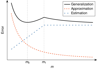
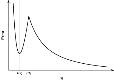
Figure 1: Risk curves for varying network width $m$ from the prediction bound (3) with $\|f^{*}\|_{\mathcal{S}}^{2}/\sigma_{\varepsilon}^{2}=1$, $d=6$, and $n=1000$. The left panel shows the decomposition of prediction error into approximation and estimation errors. The right panel shows the same plot but with larger $m$, from which it is apparent that the second valley is lower than the first.

Intuitively, the number of parameters or the network width $m$ is not an appropriate measure of model complexity for the network (2) in the overparametrized regime, and one must seek alternatives. The idea of our approach to achieving model complexity control while allowing $m$ to grow unbounded is to exploit the ridge–lasso duality of the scaled variation regularizer. On the one hand, by the positive homogeneity of the ReLU function, a reparametrization yields the equivalence of scaled variation regularization to ridge regression, which is known as (standard) weight decay in deep learning (Krogh and Hertz, 1991) and, in general, does not induce sparsity. On the other hand, a linearization of the ReLU function by parameter space partitioning transforms the regularized problem into a group lasso. This gives a key insight into the geometry of the global minima: the estimated network weights residing in the same region must be parallel to each other. Such collinearity greatly reduces the effective number of parameters and enables us to measure the model complexity in terms of the number of nonparallel directions. This implicit (within-group) formation and (between-group) breaking of symmetry lies at the heart of our theoretical analysis.

1.1 Related work

Although not the focus of this paper, approximation theory is often an integral part and first step of establishing statistical guarantees for neural networks. Sharp approximation bounds can be obtained for target functions that are well represented by two-layer neural networks, for which purpose various function spaces have been proposed. For sigmoidal networks, the seminal work of Barron (1993) considered a class of functions that have an integral representation involving the Fourier transform. The idea was further developed by, for example, Bach (2017) and Siegel and Xu (2022) to define variation spaces and norms for positively homogeneous activation functions, including ReLU. Other recent work (Ongie et al., 2020; Parhi and Nowak, 2021) has introduced an equivalent characterization of the variation space for two-layer ReLU networks via the Radon transform and has related it to more classical function spaces (Parhi and Nowak, 2022). Our choice of the target function space and its associated norm is similar to but slightly extends those of Ongie et al. (2020) and Parhi and Nowak (2022) to allow the identification of affine functions.

Generalization bounds have been derived for two-layer neural networks in certain variation spaces. Most of the existing work focuses on variational formulations of the empirical risk minimization problem. For example, Bach (2017) and Parhi and Nowak (2022) considered a variational problem by constraining the network estimator to within a ball in the function space; Parhi and Nowak (2022) showed that such network estimators are nearly minimax optimal. A representer theorem of Parhi and Nowak (2021) ensures the existence of a solution to the variational problem in the form of a finite-width network with a skip connection. However, the network width of the solution is required to be smaller than the sample size, thus providing no clue about the effect of overparametrization. One exception is the work of E, Ma and Wu (2019), which obtained generalization bounds for finite-width two-layer networks that allow the network width to grow unbounded. The $\ell_{1}$ path norm regularization that they adopted, however, induces sparsity in the network parameters, casting doubt on the implication of their results for intrinsically overparametrized networks.

Mean-field and neural tangent kernel theories are two popular frameworks for analyzing the training dynamics of two-layer neural networks in the infinite-width limit. The mean-field theory shows that the stochastic gradient descent dynamics of two-layer networks is asymptotically described by a nonlinear partial differential equation (PDE), and approximation results such as laws of large numbers and central limit theorems can be derived (Mei, Montanari and Nguyen, 2018; Sirignano and Spiliopoulos, 2020; Rotskoff and Vanden-Eijnden, 2022). The generalization behavior of the PDE model, however, is difficult to study except in some specific examples. Under a different scaling, overparametrized two-layer networks are shown to behave as their linearizations at random initialization, and optimization and generalization properties can be investigated by exploiting the neural tangent kernel (Jacot, Gabriel and Hongler, 2018) and the associated kernel methods. This “lazy training” regime (Chizat, Oyallon and Bach, 2019) entails a large performance gap between realistic and linearized networks and hence does not explain the power of fully trained neural networks (E, Ma and Wu, 2020; Ghorbani et al., 2021). Dou and Liang (2021) went a step further and developed an adaptive theory for neural network training with data-adaptive kernels. Nevertheless, the impact of adaptivity on generalization remains unclear.

Since the conceptualization of the double descent curve by Belkin et al. (2019), several theoretical models and explanations have been developed for the phenomenon. A majority of the effort has focused on linear regression and, in particular, minimum norm interpolators and ridge estimators, and has recovered the phenomenon under specific generative models for the random predictors (e.g., Belkin, Hsu and Xu, 2020; Hastie et al., 2022; Muthukumar et al., 2020). Random matrix theory is the backbone of most of these results, which concerns the high-dimensional asymptotic regime where $n,d\to\infty$ with $n\asymp d$. Similar asymptotics have been derived for random feature models (Mei and Montanari, 2022) and classification problems (Deng, Kammoun and Thrampoulidis, 2022; Liang and Sur, 2022). Li and Meng (2021) and Liang, Rakhlin and Zhai (2020) demonstrated a “multiple descent” phenomenon in infinite-dimensional linear regression and kernel ridgeless regression. Despite these important developments, it still seems difficult to isolate a general mechanism for the emergence of double descent from the oversimplified model assumptions and asymptotic regimes. Also, it remains elusive how these theories extend to realistic neural networks and fit in with our current understanding of the bias–variance trade-off (Geman, Bienenstock and Doursat, 1992; Derumigny and Schmidt-Hieber, 2023).

1.2 Organization of the paper

Section 2 introduces the definitions of two-layer ReLU networks and the target function class. Theoretical assumptions and approximation properties are also described. Section 3 presents the regularized estimation framework and formalizes the ridge–lasso duality. Our main results, including nonasymptotic generalization guarantees and minimax optimality, are developed in Section 4. Section 5 discusses the random feature model and points out its suboptimality. Section 6 provides some further discussion. Proofs are deferred to the Appendix and Supplemental Material.

2 Preliminaries

2.1 Notation

For $1\leq q<\infty$, let $\|\cdot\|_{q}$ denote the $\ell_{q}$-norm of a vector. Let $\mathbb{B}^{d}$ and $\mathbb{S}^{d-1}$ be the $\ell_{2}$ unit ball and unit sphere, respectively, in $\mathbb{R}^{d}$. For a matrix $\mathbf{B}=(\boldsymbol{\beta}_{1},\dots,\boldsymbol{\beta}_{J})$, define the $\ell_{2,1}$-norm $\|\mathbf{B}\|_{2,1}=\sum_{j=1}^{J}\|\boldsymbol{\beta}_{j}\|_{2}$. Denote by $\mathcal{M}(D)$ the set of signed measures $\alpha$ on $D$ with finite total variation $|\alpha|(D)$. In particular, the Dirac measure $\delta_{\mathbf{x}}\in\mathcal{M}(D)$ if $\mathbf{x}\in D$. For a function $f$, let $\|f\|_{L_{\infty}(D)}$ denote the $L_{\infty}$-norm on $D$, and $\|f\|_{2}$ and $\|f\|_{n}$ the $L_{2}$-norm under the distribution $\mu$ and its empirical counterpart, respectively.

2.2 Neural networks and the target function class

We consider the two-layer neural network $g(\cdot;\boldsymbol{\theta})$ with ReLU activation function and width $m$ given by (2). Let $\boldsymbol{\Theta}_{m}$ denote the parameter space. Define the scaled variation norm of the finite-width network $g(\cdot;\boldsymbol{\theta})$ by

$$\nu(\boldsymbol{\theta})=\sum_{k=1}^{m}|a_{k}|\|\mathbf{w}_{k}\|_{2},$$ (4)

where $\mathbf{w}_{k}=(\mathbf{v}_{k}^{T},b_{k})^{T}$. This regularizer was also considered by Parhi and Nowak (2021) and Parhi and Nowak (2022) for two-layer ReLU networks. It coincides with the $\ell_{1}$ path norm proposed by Neyshabur, Tomioka and Srebro (2015a) when $d$ degenerates to zero. For any $d\geq 1$, however, it is not separable in the first-layer weights and hence not a path norm. We will show in Section 3 that the scaled variation regularizer (4) has some desirable properties that are key to our theoretical analysis.

The network (2) has an integral representation with respect to a discrete signed measure. Specifically, if we define $\alpha_{m}=\sum_{k=1}^{m}a_{k}\delta_{\mathbf{w}_{k}}$, then

$$g(\mathbf{x};\boldsymbol{\theta})=\int_{\mathbb{R}^{d+1}}\bigl{(}\sigma(\mathbf{v}^{T}\mathbf{x}+b)-\sigma(b)\bigr{)}\,d\alpha_{m}(\mathbf{w})+g(\mathbf{0};\boldsymbol{\theta}).$$

Motivated by this observation, we can naturally represent an infinite-width two-layer ReLU network associated with a signed measure $\alpha\in\mathcal{M}(\mathbb{R}^{d+1})$ as

$$g_{\alpha}(\mathbf{x})=\int_{\mathbb{R}^{d+1}}\bigl{(}\sigma(\mathbf{v}^{T}\mathbf{x}+b)-\sigma(b)\bigr{)}\,d\alpha(\mathbf{w})+g_{\alpha}(\mathbf{0}).$$

For $g_{\alpha}(\cdot)$ to be well defined, a sufficient condition is

$$\int_{\mathbb{R}^{d+1}}\|\mathbf{v}\|_{2}\,d|\alpha|(\mathbf{w})<\infty,$$

since by the Lipschitz continuity of the ReLU function, $|\sigma(\mathbf{v}^{T}\mathbf{x}+b)-\sigma(b)|\leq|\mathbf{v}^{T}\mathbf{x}|\leq\|\mathbf{v}\|_{2}\|\mathbf{x}\|_{2}$. Treating functions that differ by a constant as identical, we consider the space of functions modulo constants

$$\mathcal{G}=\biggl{\{}\mathbf{x}\mapsto\int_{\mathbb{R}^{d+1}}\bigl{(}\sigma(\mathbf{v}^{T}\mathbf{x}+b)-\sigma(b)\bigr{)}\,d\alpha(\mathbf{w}):\int_{\mathbb{R}^{d+1}}\|\mathbf{v}\|_{2}\,d|\alpha|(\mathbf{w})<\infty\biggr{\}}.$$ (5)

Interestingly, there is a one-to-one correspondence between $\mathcal{G}$ and $\mathcal{M}_{2}(\mathbb{R}^{d+1})\equiv\bigl{\{}\alpha\in\mathcal{M}(\mathbb{R}^{d+1}):\int_{\mathbb{R}^{d+1}}\|\mathbf{v}\|_{2}\,d|\alpha|(\mathbf{w})<\infty\bigr{\}}$. Moreover, functions in $\mathcal{G}$ are exactly those that can be approximated by two-layer ReLU networks with finite scaled variation norm. A formal statement is given by Proposition LABEL:prop:functionspace2 in the Supplementary Material. To equip the function space $\mathcal{G}$ with a norm, we introduce the following definition.

Definition 1.

The $\mathcal{S}$-norm of $f\in\mathcal{G}$ is defined as $\|f\|_{\mathcal{S}}=\int_{\mathbb{R}^{d+1}}\|\mathbf{v}\|_{2}\,d|\alpha_{f}|(\mathbf{w})$, where the signed measure $\alpha_{f}\in\mathcal{M}_{2}(\mathbb{R}^{d+1})$ is uniquely determined by

$$f(\mathbf{x})=\int_{\mathbb{R}^{d+1}}\bigl{(}\sigma(\mathbf{v}^{T}\mathbf{x}+b)-\sigma(b)\bigr{)}\,d\alpha_{f}(\mathbf{w})+f(\mathbf{0}).$$

Clearly, the $\mathcal{S}$-norm is a functional version of the scaled variation norm except for the omission of the bias term owing to the centering by $\sigma(b)$. In fact, the $\mathcal{S}$-norm of a finite-width two-layer ReLU network $g(\cdot;\boldsymbol{\theta})$ is $\|g(\cdot;\boldsymbol{\theta})\|_{\mathcal{S}}=\sum_{k=1}^{m}|a_{k}|\|\mathbf{v}_{k}\|_{2}$, which is bounded above by the scaled variation norm (4).

Our definition of the target function space is inspired by and related to several previously studied spaces for two-layer neural networks. In particular, $\mathcal{G}$ is equivalent to the bounded variation spaces in the Radon domain considered by Ongie et al. (2020) and Parhi and Nowak (2021) and the variation spaces considered by Bach (2017) and Siegel and Xu (2022), which in turn contain the spectral Barron spaces and Sobolev spaces (Klusowski and Barron, 2018; Parhi and Nowak, 2022). Our definition of the $\mathcal{S}$-norm is more transparent in that it is defined explicitly as a functional of $\alpha_{f}$, a uniquely determined signed measure. Moreover, it slightly improves on previous proposals in several respects. Notably, for an affine function $f_{\boldsymbol{\beta}}(\mathbf{x})=\boldsymbol{\beta}^{T}\mathbf{x}+c$, $\|f_{\boldsymbol{\beta}}\|_{\mathcal{S}}=2\|\boldsymbol{\beta}\|_{2}$ instead of being zero. This has two important consequences: (i) the $\mathcal{S}$-norm is a norm rather than a seminorm; and (ii) there is no need to introduce a skip connection in a representer theorem (cf. Ongie et al., 2020; Parhi and Nowak, 2021). The latter is compatible with deep learning practice since skip connections are only necessary in deep neural networks such as residual networks (He et al., 2016). More mathematical details can be found in Section LABEL:sec:target_function of the Supplementary Material.

2.3 Assumptions

We consider the nonparametric regression model (1) and impose the following conditions:

$f^{*}\in\mathcal{G}_{M}\equiv\{f\in\mathcal{G}:\|f\|_{\mathcal{S}}\leq M\}$ for some constant $M>0$;

$\mathbf{x}_{i}\sim\mu$ independently, where $\mu$ is supported in $\mathbb{B}^{d}$;

$\varepsilon_{i}\sim N(0,\sigma_{\varepsilon}^{2})$ independently and are independent of $\mathbf{x}_{i}$.

Condition (2.3) is mild and standard in the machine learning literature since the predictors are usually bounded and can be normalized. Under Condition (2.3), it suffices to consider the restrictions of functions in $\mathcal{G}$ to $\mathbb{B}^{d}$; denote the space of such restrictions by $\mathcal{G}(\mathbb{B}^{d})$. An important consequence from Corollary LABEL:cor:restriction in the Supplementary Material is that, for any $f\in\mathcal{G}(\mathbb{B}^{d})$, there exists a signed measure $\widetilde{\alpha}_{f}\in\mathcal{M}(\mathbb{S}^{d-1}\times[-1,1])$ such that

$$f(\mathbf{x})=\int_{\mathbb{S}^{d-1}\times[-1,1]}\sigma(\mathbf{v}^{T}\mathbf{x}+b)\,d\widetilde{\alpha}_{f}(\mathbf{w})+c,\quad\mathbf{x}\in\mathbb{B}^{d}.$$ (6)

Compared with a similar integral representation in Parhi and Nowak (2022, Remark 3), note that no skip connection appears in (6). Thus, functions in $\mathcal{G}(\mathbb{B}^{d})$ have a simpler integral representation

$$\mathcal{G}(\mathbb{B}^{d})=\biggl{\{}\mathbf{x}\mapsto\int_{\mathbb{S}^{d-1}\times[-1,1]}\sigma(\mathbf{v}^{T}\mathbf{x}+b)\,d\alpha(\mathbf{w}):|\alpha|(\mathbb{S}^{d-1}\times[-1,1])<\infty\biggr{\}},$$

which will allow us to obtain a sharp approximation bound.

2.4 Approximation properties

Approximation rates for two-layer neural networks of width $m$ have been derived in various function spaces. A classical probabilistic argument, first applied to neural networks by Barron (1993), yields an approximation rate of $O(1/\sqrt{m})$ in the $L_{2}$-norm; see also Jones (1992) and Siegel and Xu (2020). The approximation rate has been improved by Makovoz (1996), Bach (2017), and Klusowski and Barron (2018), among others. In particular, Bach (2017) obtained an $O(m^{-(d+3)/(2d)})$ rate in the $L_{\infty}$-norm by using a result from geometric discrepancy theory (Matoušek, 1996); Siegel and Xu (2022) showed that this rate is sharp and not improvable. We have the following approximation result for functions in $\mathcal{G}_{M}$, which is a direct consequence of Bach (2017, Proposition 1) and the integral representation (6).

Theorem 1.

For any $f\in\mathcal{G}_{M}$, there exists a network $g(\cdot;\boldsymbol{\theta})$ of width $m$ in the form of (2) such that $\nu(\boldsymbol{\theta})\leq 6\|f\|_{\mathcal{S}}$ and

$$\|f-g(\cdot;\boldsymbol{\theta})\|_{L_{\infty}(\mathbb{B}^{d})}\leq C\|f\|_{\mathcal{S}}m^{-(d+3)/(2d)}$$

for some constant $C>0$ depending only on $d$.

The construction in Theorem 1 has a tight control on the scaled variation norm of the network parameter. This suggests using the scaled variation norm as a regularizer for the network estimation problem, as we will discuss in the next section.

3 Methodology and the ridge–lasso duality

In this section we introduce our regularized estimation problem and formalize the notion of the ridge–lasso duality through two different reparametrizations.

3.1 Regularized estimation

In order to learn $f^{*}$ from the training sample, we adopt the penalized empirical risk minimization (ERM) framework and seek to minimize

$$J_{n}(\boldsymbol{\theta};\lambda)=\frac{1}{2n}\sum_{i=1}^{n}\bigl{(}y_{i}-g(\mathbf{x}_{i};\boldsymbol{\theta})\bigr{)}^{2}+\lambda\nu(\boldsymbol{\theta}),$$

where $g(\cdot;\boldsymbol{\theta})$ is the two-layer ReLU network of width $m$ in (2), $\nu(\boldsymbol{\theta})$ is the scaled variation norm in (4), and $\lambda>0$ is a regularization parameter. The regularized network estimator is given by $g(\cdot;\widehat{\boldsymbol{\theta}})$, where

$$\widehat{\boldsymbol{\theta}}=\operatorname*{\arg\min}_{\boldsymbol{\theta}\in\boldsymbol{\Theta}_{m}}J_{n}(\boldsymbol{\theta};\lambda).$$ (7)

In a related work, Parhi and Nowak (2022) studied a variational problem in the variation space associated with two-layer ReLU networks, where regularization is imposed as a constraint on the variation norm of the network function. A representer theorem guarantees the existence of a finitely supported solution of width $m\leq n-(d+1)$ to the variational problem. However, the finite-dimensional network learning problem is equivalent to the variational problem only when $m\geq n-(d+1)$. See their Theorem 5 and Section III.B. Therefore, their results still fall within the underparametrized regime and do not fully characterize the influence of the network width. By contrast, we provide a direct attack on the finite-dimensional network learning problem (7) and allow the network width $m$ to vary freely.

3.2 Equivalence to ridge regression

In this and the next subsections, we explore some useful reformulations of the optimization problem (7), which allow the scaled variation regularizer, when coupled with the ReLU function, to inherit some crucial properties from ridge regression (Hoerl, 2020) and the group lasso (Yuan and Lin, 2006), two familiar forms of regularization in statistics. We start by recasting (7) as the $\ell_{2}$-regularized ERM problem

$$\widehat{\boldsymbol{\theta}}_{\ell_{2}}=\operatorname*{\arg\min}_{\boldsymbol{\theta}\in\boldsymbol{\Theta}_{m}}\Biggl{\{}\frac{1}{2n}\sum_{i=1}^{n}\bigl{(}y_{i}-g(\mathbf{x}_{i};\boldsymbol{\theta})\bigr{)}^{2}+\frac{\lambda}{2}\sum_{k=1}^{m}(a_{k}^{2}+\|\mathbf{w}_{k}\|_{2}^{2})\Biggr{\}}.$$ (8)

To see this, consider the reparametrization $\widetilde{\boldsymbol{\theta}}=\mathcal{T}_{1}(\boldsymbol{\theta})$ defined by

$$\widetilde{a}_{k}=a_{k}\sqrt{\frac{\|\mathbf{w}_{k}\|_{2}}{|a_{k}|}},\qquad\widetilde{\mathbf{w}}_{k}=\mathbf{w}_{k}\sqrt{\frac{|a_{k}|}{\|\mathbf{w}_{k}\|_{2}}}$$

if $|a_{k}|\|\mathbf{w}_{k}\|_{2}\neq 0$, and $(\widetilde{a}_{k},\widetilde{\mathbf{w}}_{k}^{T})=\mathbf{0}$ otherwise. After the reparametrization, we have $|\widetilde{a}_{k}|=\|\widetilde{\mathbf{w}}_{k}\|_{2}$ and the regularizer becomes

$$\sum_{k=1}^{m}|\widetilde{a}_{k}|\|\widetilde{\mathbf{w}}_{k}\|_{2}=\frac{1}{2}\sum_{k=1}^{m}(\widetilde{a}_{k}^{2}+\|\widetilde{\mathbf{w}}_{k}\|_{2}^{2}).$$

Meanwhile, the positive homogeneity of the ReLU function implies that $a_{k}\sigma((\mathbf{x}_{k}^{T},1)\mathbf{w}_{k})=\widetilde{a}_{k}\sigma((\mathbf{x}_{k}^{T},1)\widetilde{\mathbf{w}}_{k})$, so that the network function is invariant under the reparametrization. Note further that any solution $\widehat{\boldsymbol{\theta}}_{\ell_{2}}$ to the problem (8) must satisfy $\widehat{\boldsymbol{\theta}}_{\ell_{2}}=\mathcal{T}_{1}(\widehat{\boldsymbol{\theta}}_{\ell_{2}})$, because otherwise it could be improved by a rescaling. Using these facts, we obtain the following equivalence result.

Proposition 1.

Any solution $\widehat{\boldsymbol{\theta}}_{\ell_{2}}$ to the optimization problem (8) is a solution to the problem (7). Conversely, if $\widehat{\boldsymbol{\theta}}$ is a solution to the optimization problem (7), then $\mathcal{T}_{1}(\widehat{\boldsymbol{\theta}})$ is a solution to the problem (8).

Proposition 1 says that the solutions to the $\ell_{2}$-regularized problem lie on a submanifold of the solution manifold of the original problem that is invariant under the reparametrization $\mathcal{T}_{1}$. What is the implication of this equivalence for neural network training dynamics with, for example, gradient descent? The following result assures us that the gradient flow trajectories for the two problems are indeed identical when initialized with a reparametrization $\mathcal{T}_{1}$.

Proposition 2.

Consider the gradient flow for the optimization problem (7) defined by

$$\frac{d}{dt}\boldsymbol{\theta}(t)=-\nabla_{\boldsymbol{\theta}}J_{n}(\boldsymbol{\theta}(t);\lambda)$$

and for the problem (8) defined similarly, both initialized at $\boldsymbol{\theta}(0)=\mathcal{T}_{1}(\boldsymbol{\theta}_{0})$ for an arbitrary $\boldsymbol{\theta}_{0}\in\boldsymbol{\Theta}_{m}$. Then the trajectories of the two gradient flows coincide.

Observations similar to Proposition 1 have been noted in slightly different forms by, for example, Neyshabur, Tomioka and Srebro (2015b, Theorem 1) and Parhi and Nowak (2021, Theorem 8). Initialization with the reparametrization $\mathcal{T}_{1}$ and its stationarity along the gradient flow have been exploited by Dou and Liang (2021) for studying the $\ell_{2}$-regularized ERM problem, where it is referred to as a “balanced condition.” The messages of the above results are twofold. First, since $\ell_{2}$ regularization does not induce entrywise sparsity in the parameters (but see Srebro, Rennie and Jaakkola (2004) for an unusual example where it does induce sparsity in spectral structures), we are assured that a sufficiently wide two-layer network can be intrinsically overparametrized. Second, several implicit regularization strategies for deep learning, such as noise injection and early stopping, have been shown to be equivalent to $\ell_{2}$ regularization (Bishop, 1995; Sjöberg and Ljung, 1995), which may help bridge the gap between our method and implicit regularization.

3.3 Connection to the group lasso

One major obstacle in analyzing the generalization performance of neural networks is the excessive redundancy and nonidentifiability of the network parameters under the usual nonconvex formulation. The ReLU activation function, on the other hand, is simple enough in that it reduces to a linear function once the sign of $\mathbf{v}_{k}^{T}\mathbf{x}+b_{k}$ is fixed. This naturally suggests a partitioning of the parameter space $\mathbb{R}^{d+1}$ for $\mathbf{w}$ by certain hyperplanes into regions within which the signs of $\mathbf{x}_{i}^{T}\mathbf{v}+b$ are all determined. The partition will then allow us to reveal a strong symmetry in the estimated network parameters and recast the optimization problem (7) in a group lasso form, which will be convenient for the derivation of generalization properties in the next section.

Specifically, denote by $\mathbf{X}=((\mathbf{x}_{1}^{T},1)^{T},\dots,(\mathbf{x}_{n}^{T},1)^{T})^{T}$ the $n\times(d+1)$ design matrix, and $\mathbf{D}=\operatorname{diag}(I(\mathbf{X}\mathbf{w}\geq 0))$ the diagonal indicator matrix for the positivity of $\mathbf{X}\mathbf{w}$. Consider the hyperplanes in $\mathbb{R}^{d+1}$ passing through the origin and orthogonal to $\mathbf{x}_{i}$, defined by $\mathbf{x}_{i}^{T}\mathbf{v}+b=0$. These $n$ hyperplanes divide the parameter space $\mathbb{R}^{d+1}$ into finitely many regions, denoted by $R_{1},\dots,R_{p}$, such that $\mathbf{D}$ stays constant over (the interior of) each $R_{j}$. It is well known (Cover, 1965, Theorem 2) that the number of these regions

$$p\leq 2\sum_{j=0}^{d}\binom{n-1}{j}\leq 2n^{d},$$ (9)

where the first upper bound is sharp when $\mathbf{X}$ has full rank. Taking into account the sign of $a$, we thus partition the parameter space $\mathbb{R}^{d+2}$ for $(a,\mathbf{w}^{T})^{T}$ into $2p$ regions

$$Q_{j}=[0,\infty)\times R_{j},\quad Q_{p+j}=(-\infty,0)\times R_{j},\quad j=1,\dots,p,$$

and define $\mathbf{D}_{p+j}=-\mathbf{D}_{j}$. Clearly, $R_{j}$ and $Q_{j}$ are convex cones. The linearity of the ReLU function over each $Q_{j}$ and the optimality of $\widehat{\boldsymbol{\theta}}$ entail the following collinearity property.

Proposition 3.

For any solution $\widehat{\boldsymbol{\theta}}=(\widehat{a}_{1},\dots,\widehat{a}_{m},\widehat{\mathbf{w}}_{1}^{T},\dots,\widehat{\mathbf{w}}_{m}^{T})^{T}$ to the optimization problem (7), if $(\widehat{a}_{k},\widehat{\mathbf{w}}_{k}^{T})^{T}$ and $(\widehat{a}_{\ell},\widehat{\mathbf{w}}_{\ell}^{T})^{T}$ lie in the interior of the same cone $Q_{j}$, then $\widehat{\mathbf{w}}_{k}$ and $\widehat{\mathbf{w}}_{\ell}$ must be collinear, that is, $\widehat{\mathbf{w}}_{k}=c_{0}\widehat{\mathbf{w}}_{\ell}$ for some constant $c_{0}>0$.

Define $S_{j}=\{1\leq k\leq m:(a_{k},\mathbf{w}_{k}^{T})^{T}\in Q_{j}\}$, $s_{j}=1$, and $s_{p+j}=-1$ for $j=1,\dots,p$. To understand why the collinearity must hold, note that the “conewise collinearization” $\widetilde{\boldsymbol{\theta}}=\mathcal{T}_{2}(\boldsymbol{\theta})$ defined by

$$\widetilde{a}_{k}=s_{j},\quad\widetilde{\mathbf{w}}_{k}=\frac{1}{|S_{j}|}\sum_{\ell\in S_{j}}|a_{\ell}|\mathbf{w}_{\ell},\quad k\in S_{j}$$ (10)

does not change the value of the network function on the training sample, but would yield a smaller scaled variation norm by the triangle inequality if the network weights in $Q_{j}$ were not all collinear. Proposition 3 provides a useful geometric insight into the regularization effect of scaled variation norm: it favors the most symmetric (yet not parsimonious) representation among many equivalent parametrizations within the same cone.

The parameter redundancy suggested by Proposition 3 motivates us to collect the network weights falling within the same cone and define the aggregated parameters $\mathbf{B}(\boldsymbol{\theta})=(\boldsymbol{\beta}_{1}(\boldsymbol{\theta}),\dots,\boldsymbol{\beta}_{2p}(\boldsymbol{\theta}))$ with

$$\boldsymbol{\beta}_{j}(\boldsymbol{\theta})=\sum_{k\in S_{j}}|a_{k}|\mathbf{w}_{k}.$$

With this new set of parameters, the network function on the training sample can be written in the linear form

$$\sum_{k=1}^{m}a_{k}\sigma(\mathbf{X}\mathbf{w}_{k})=\sum_{j=1}^{2p}\mathbf{D}_{j}\mathbf{X}\boldsymbol{\beta}_{j}(\boldsymbol{\theta}),$$ (11)

where $\sigma(\cdot)$ applies componentwise. For any $\boldsymbol{\theta}\in\boldsymbol{\Theta}_{m}$, the triangle inequality implies that

$$\|\mathbf{B}(\boldsymbol{\theta})\|_{2,1}=\sum_{j=1}^{2p}\|\boldsymbol{\beta}_{j}(\boldsymbol{\theta})\|_{2}\leq\sum_{j=1}^{2p}\sum_{k\in S_{j}}|a_{k}|\|\mathbf{w}_{k}\|_{2}=\nu(\boldsymbol{\theta}),$$

where the equality holds under the reparametrization $\mathcal{T}_{2}$. In particular, since the estimator $\widehat{\boldsymbol{\theta}}$ satisfies the collinearity property, we can replace $\nu(\widehat{\boldsymbol{\theta}})$ by $\|\mathbf{B}(\widehat{\boldsymbol{\theta}})\|_{2,1}$ and reformulate (7) as a group lasso problem. Denote by $\mathbf{y}=(y_{1},\dots,y_{n})^{T}$ the response vector. We summarize the above discussion in the following proposition.

Proposition 4.

For any $\boldsymbol{\theta}\in\boldsymbol{\Theta}_{m}$, the reparametrization $\widetilde{\boldsymbol{\theta}}=\mathcal{T}_{2}(\boldsymbol{\theta})$ defined in (10) satisfies $g(\mathbf{x}_{i};\widetilde{\boldsymbol{\theta}})=g(\mathbf{x}_{i};\boldsymbol{\theta})$ for $i=1,\dots,n$ and $\|\mathbf{B}(\widetilde{\boldsymbol{\theta}})\|_{2,1}=\nu(\widetilde{\boldsymbol{\theta}})\leq\nu(\boldsymbol{\theta})$. Furthermore, the solution $\widehat{\boldsymbol{\theta}}$ to the optimization problem (7) satisfies

$$J_{n}(\widehat{\boldsymbol{\theta}};\lambda)=\frac{1}{2n}\biggl{\|}\mathbf{y}-\sum_{j=1}^{2p}\mathbf{D}_{j}\mathbf{X}\boldsymbol{\beta}_{j}(\widehat{\boldsymbol{\theta}})\biggr{\|}_{2}^{2}+\lambda\|\mathbf{B}(\widehat{\boldsymbol{\theta}})\|_{2,1}.$$

The group lasso formulation allows for borrowing ideas from high-dimensional statistics to derive generalization bounds. We emphasize, however, that the parameter space partition and the resulting group structure are data-adaptive and not known a priori. Hence, despite the connection to the group lasso, two-layer ReLU networks are radically different from linear models and hold the potential for better generalization.

Similar connections between $\ell_{2}$-regularized two-layer ReLU networks and the group lasso have been explored by Pilanci and Ergen (2020) and Wang, Lacotte and Pilanci (2022) from a purely optimization standpoint. A complete equivalence result, however, requires $m$ to be sufficiently large; see Theorem 1 of Pilanci and Ergen (2020). Our key observation is that for our purposes it suffices to have the weaker result of Proposition 4, which places no restriction on the minimum network width.

4 Main results

In this section we establish statistical guarantees for two-layer ReLU networks. In Section 4.1 we present nonasymptotic bounds on the prediction error of the regularized network estimator, and in Section 4.2 show that they are nearly minimax optimal.

4.1 Nonasymptotic generalization bounds

For the nonparametric regression model (1) and the regularized network estimator $g(\cdot;\widehat{\boldsymbol{\theta}})$ defined by (7), we are interested in bounding the empirical error

$$\|g(\cdot;\widehat{\boldsymbol{\theta}})-f^{*}\|_{n}^{2}=\frac{1}{n}\sum_{i=1}^{n}\bigl{(}g(\mathbf{x}_{i};\widehat{\boldsymbol{\theta}})-f^{*}(\mathbf{x}_{i})\bigr{)}^{2}$$

in the fixed design case, and the prediction (or generalization) error

$$\|g(\cdot;\widehat{\boldsymbol{\theta}})-f^{*}\|_{2}^{2}=\mathbb{E}_{\mathbf{x}\sim\mu}\bigl{(}g(\mathbf{x};\widehat{\boldsymbol{\theta}})-f^{*}(\mathbf{x})\bigr{)}^{2}$$

in the random design case. Our main techniques for proving the nonasymptotic bounds are inspired by and synthesize those in previous work on high-dimensional linear models and two-layer neural networks. We first note that the technical arguments best suited to the underparametrized and overparametrized regimes may be rather different. For underparametrized networks, complexity control via metric entropy (e.g., Barron, 1994; Parhi and Nowak, 2022) can be effective and give sharp bounds. Moving into the overparametrized regime, however, entropy-based bounds tend to be too loose and pessimistic since they do not take into account the parameter redundancy growing with the network width. We therefore turn to the group lasso formulation outlined in Section 3.3 and borrow ideas from (group) $\ell_{1}$-regularized linear regression and norm-based complexity control. Our first result concerns the empirical error of the regularized network estimator.

Theorem 2.

Under Conditions (2.3) and (2.3) and the assumption that $\max_{i}\|\mathbf{x}_{i}\|_{2}\leq 1$, the regularized network estimator $g(\cdot;\widehat{\boldsymbol{\theta}})$ with $\lambda=C_{1}\sigma_{\varepsilon}\sqrt{d\log n/n}$ satisfies

$$\|g(\cdot;\widehat{\boldsymbol{\theta}})-f^{*}\|_{n}^{2}\leq C\biggl{\{}\|f^{*}\|_{\mathcal{S}}^{2}m^{-(d+3)/d}+(\sigma_{\varepsilon}^{2}+\|f^{*}\|_{\mathcal{S}}^{2})\sqrt{\frac{d\log n}{n}}\biggr{\}}$$ (12)

with probability at least $1-O(n^{-C_{2}})$, and

$$\mathbb{E}\|g(\cdot;\widehat{\boldsymbol{\theta}})-f^{*}\|_{n}^{2}\leq C\biggl{\{}\|f^{*}\|_{\mathcal{S}}^{2}m^{-(d+3)/d}+(\sigma_{\varepsilon}^{2}+\|f^{*}\|_{\mathcal{S}}^{2})\sqrt{\frac{d\log n}{n}}\biggr{\}},$$ (13)

for some constants $C_{1},C_{2},C>0$.

Throughout this section, the constants are independent of $m$ and $n$, but may depend on $d$, $M$, and $\sigma_{\varepsilon}$; we have suppressed the dependence for simplicity, which can be made explicit by inspecting our proofs. Our technique for proving Theorem 2 differs from the standard group lasso theory for sparse linear regression in two aspects. First, it requires an extension of the theory to the case where the linear model is only approximate, as discussed in, for example, Bühlmann and van de Geer (2011, Section 6.2.3). Here the linear model represents the reparametrized two-layer neural network, whose approximation error has been given by Theorem 1. Second, and more importantly, there is no guarantee that this linear model will be sparse or its design will satisfy a compatibility or restricted eigenvalue condition that is often imposed in high-dimensional linear regression. As a result, we can only prove a prediction bound at a slower rate, which is analogous to those for the lasso obtained by Bühlmann and van de Geer (2011, Corollary 6.1) and Bartlett, Mendelson and Neeman (2012).

The error bounds in Theorem 2 decompose into a bias term or approximation error that arises from using a finite-width neural network to approximate the nonparametric model (1), and a variance term or estimation error that accounts for the variability in estimating the finite-width network. The most surprising fact about this decomposition is that there is no trade-off between the two terms: as the network width $m$ increases, the bias always decreases while the variance remains constant. To appreciate why this is possible, note first that the variance scales as $O(\sqrt{\log p/n})$ as a consequence of the lack of parameter identifiability. Moreover, the effective dimension $p$ is bounded by $O(n^{d})$ from (9), which does not depend on the network width $m$. In fact, when the design matrix $\mathbf{X}$ is of rank $r<n$, one can further replace $d$ by $r$ (Cover, 1965). In other words, no matter how large $m$ grows, the number of distinct (nonparallel) features extracted by the first layer of the network is finite, leading to an upper bound for the variance. This result extends beyond the classical bias–variance trade-off and demonstrates the virtues of overparametrization in two-layer neural networks.

Combining Theorem 2 with a maximal inequality, we obtain similar bounds on the prediction error of the regularized network estimator.

Theorem 3.

Under Conditions (2.3)–(2.3), if $m\geq C_{1}\{n/(d\log n)\}^{d/(2(d+3))}$, then the regularized network estimator $g(\cdot;\widehat{\boldsymbol{\theta}})$ with $\lambda=\lambda_{1}\equiv C_{2}\sigma_{\varepsilon}\sqrt{d\log n/n}$ satisfies

$$\|g(\cdot;\widehat{\boldsymbol{\theta}})-f^{*}\|_{2}^{2}\leq C\biggl{\{}\|f^{*}\|_{\mathcal{S}}^{2}m^{-(d+3)/d}+(\sigma_{\varepsilon}^{2}+\|f^{*}\|_{\mathcal{S}}^{2})\sqrt{\frac{d\log n}{n}}\biggr{\}}$$ (14)

with probability at least $1-O(n^{-C_{3}})$, and

$$\mathbb{E}\|g(\cdot;\widehat{\boldsymbol{\theta}})-f^{*}\|_{2}^{2}\leq C\biggl{\{}\|f^{*}\|_{\mathcal{S}}^{2}m^{-(d+3)/d}+(\sigma_{\varepsilon}^{2}+\|f^{*}\|_{\mathcal{S}}^{2})\sqrt{\frac{d\log n}{n}}\biggr{\}},$$ (15)

for some constants $C_{1},C_{2},C_{3},C>0$ and sufficiently large $n$.

It is worthwhile to compare our results with those in the literature on overparametrized two-layer ReLU networks. Recent research has focused on the neural tangent kernel regime and showed that sufficiently wide two-layer ReLU networks trained by gradient descent with random initialization achieve a generalization error of $O(n^{-1/2})$ up to logarithmic factors; see, for example, Arora et al. (2019), E, Ma and Wu (2020), and Ji and Telgarsky (2020). While these results deliver roughly the same rates as ours, the target functions they considered fall in a certain reproducing kernel Hilbert space, which constitutes only a small subset of our target function space. In addition, our analysis is algorithm-independent and is valid for any global optimum.

E, Ma and Wu (2019) considered explicit regularization for two-layer ReLU networks and obtained generalization bounds of $O(m^{-1}+n^{-1/2})$ up to logarithmic factors, which are of a similar nature to ours. However, several differences are notable. First, they employed the $\ell_{1}$ path norm, which penalizes on the $\ell_{1}$-norm of the first-layer weights and promotes sparsity. Accordingly, they considered the so-called Barron space

$$\mathcal{B}_{2}=\biggl{\{}\mathbf{x}\mapsto\int_{\mathbb{S}_{1}^{d-1}}a(\mathbf{v})\sigma(\mathbf{v}^{T}\mathbf{x})\,d\rho(\mathbf{v}):\int_{\mathbb{S}_{1}^{d-1}}a(\mathbf{v})^{2}\,d\rho(\mathbf{v})<\infty\biggr{\}},$$

where $\mathbb{S}_{1}^{d-1}$ is the $\ell_{1}$ unit sphere in $\mathbb{R}^{d}$. To compare with our definition of $\mathcal{G}$ in (5), let $d\alpha_{\rho}(\mathbf{w})=a(\mathbf{v})I(\mathbf{v}\in\mathbb{S}_{1}^{d-1},b=0)\,d\rho(\mathbf{v})$, where $I(\cdot)$ is the indicator function. Then

$$\int_{\mathbb{R}^{d+1}}\|\mathbf{v}\|_{2}\,d|\alpha_{\rho}|(\mathbf{w})\leq\sqrt{d}\int_{\mathbb{S}_{1}^{d-1}}|a(\mathbf{v})|\,d\rho(\mathbf{v})\leq\sqrt{d}\biggl{(}\int_{\mathbb{S}_{1}^{d-1}}a(\mathbf{v})^{2}\,d\rho(\mathbf{v})\biggr{)}^{1/2}<\infty$$

by the Cauchy–Schwarz inequality. Thus, we see that $\mathcal{B}_{2}$ is a subset of our target function space $\mathcal{G}$. Furthermore, they resorted to a truncated risk to deal with the noisy case, which introduces some technicalities that seem unnecessary.

The group lasso approach and the size-independent upper bound (9) for $p$, albeit effective in the overparametrized regime, tend to overestimate the variance for sufficiently narrow networks. In this case, a standard metric entropy argument may be more appropriate and give a sharper estimate of the variance that increases with the network width. Adapting this argument to our regularization problem yields the following result, which demonstrates a classical bias–variance trade-off.

Theorem 4.

Under Conditions (2.3)–(2.3), if $m<n/(d\log n)$, then the regularized network estimator $g(\cdot;\widehat{\boldsymbol{\theta}})$ with $\lambda=\lambda_{2}\equiv C_{1}\sigma_{\varepsilon}\max(m^{-(d+3)/d},md\log n/n)$ satisfies

$$\|g(\cdot;\widehat{\boldsymbol{\theta}})-f^{*}\|_{2}^{2}\leq C\biggl{\{}\|f^{*}\|_{\mathcal{S}}^{2}m^{-(d+3)/d}+(\sigma_{\varepsilon}^{2}+\|f^{*}\|_{\mathcal{S}}^{2})\frac{md\log n}{n}\biggr{\}}$$

with probability at least $1-O(n^{-C_{2}})$ for some constants $C_{1},C_{2},C>0$.

The proof technique used for Theorem 4 differs substantially from those in previous work, since we are analyzing a penalized rather than constrained problem and do not impose any boundedness constraints on the network function or parameters; cf. Schmidt-Hieber (2020), Farrell, Liang and Misra (2021), and Parhi and Nowak (2022).

Finally, noting that the ranges of allowable $m$ in Theorems 3 and 4 partially overlap, we put them together to obtain a complete picture of the generalization behavior of two-layer ReLU networks, as stated in the following encompassing result.

Theorem 5.

Under Conditions (2.3)–(2.3), the regularized network estimator $g(\cdot;\widehat{\boldsymbol{\theta}})$ with $\lambda=\min(\lambda_{1},\lambda_{2})$, where $\lambda_{1}$ and $\lambda_{2}$ are defined in Theorems 3 and 4, respectively, satisfies

$$\|g(\cdot;\widehat{\boldsymbol{\theta}})-f^{*}\|_{2}^{2}\leq C\biggl{\{}\|f^{*}\|_{\mathcal{S}}^{2}m^{-(d+3)/d}+(\sigma_{\varepsilon}^{2}+\|f^{*}\|_{\mathcal{S}}^{2})\min\biggl{(}\sqrt{\frac{d\log n}{n}},\frac{md\log n}{n}\biggr{)}\biggr{\}}$$

with probability at least $1-O(n^{-C_{1}})$ for some constants $C_{1},C>0$ and sufficiently large $n$.

The implications of Theorem 5 have been discussed in the Introduction. In particular, it gives rise to the double descent risk curve illustrated in Figure 1 and provides a simple yet appealing explanation for the curious phenomenon. In the underparametrized regime, the network estimator behaves as the usual nonparametric methods, with the network width $m$ controlling the trade-off between bias and variance. A too small or too large $m$ will result in an inferior performance, and a narrow valley around $m_{0}\asymp(n/(d\log n))^{d/(2d+3)}$ lies in between. As $m$ continues to increase and exceeds some threshold $m_{1}\asymp\sqrt{n/(d\log n)}$, the intrinsic model complexity and hence the variance of the network estimator become saturated and remain constant, while the bias diminishes consistently. This leads to a second, flat valley extending toward infinity.

Comparisons between the two valleys yield further insights. Asymptotically, the convergence rate of the first valley or underparametrized minimum risk, $O((d\log n/n)^{(d+3)/(2d+3)})$, is slightly smaller than that of the second valley or overparametrized minimum risk, $O(\sqrt{d\log n/n})$. In finite samples, however, this comparison can be reversed. A little algebra shows that the second valley is lower than the first whenever

$$\kappa\equiv\frac{\|f^{*}\|_{\mathcal{S}}^{2}}{\sigma_{\varepsilon}^{2}+\|f^{*}\|_{\mathcal{S}}^{2}}>\biggl{(}\frac{1}{2}\biggr{)}^{(2d+3)/d}\biggl{(}\frac{n}{d\log n}\biggr{)}^{3/(2d)}.$$ (16)

When $d\gg\log n$, the above condition approximately becomes $\kappa>1/4$, or the signal-to-noise ratio $\|f^{*}\|_{\mathcal{S}}^{2}/\sigma_{\varepsilon}^{2}=\kappa/(1-\kappa)>1/3$. An example with $\kappa=1$, $d=6$, and $n=1000$ was given in Figure 1. This makes intuitive sense since the reduction in approximation error plays a more important role when the signal is stronger. From the practitioner’s perspective, the overparametrized regime is also more attractive in that it provides an infinitely wide sweet spot that avoids the choice of an optimal network width.

4.2 Minimax lower bounds

We have revealed that the risk curve of our estimator has two valleys. The convergence rate of the first valley is known to be minimax optimal over the function class $\mathcal{G}_{M}$ (Parhi and Nowak, 2022). In fact, the underparametrized result (Theorem 4) relies crucially on the assumption that $M$ is finite; otherwise, the entropy calculations may be affected. In this subsection, we investigate the optimality of the second valley. Although it cannot be optimal over $\mathcal{G}_{M}$, we will show that it is nearly minimax optimal over the larger function class $\mathcal{G}$.

To gain intuition for the optimal rate, for any probability measure $\rho$ on $\mathbb{S}^{d-1}\times[-1,1]$, we consider the reproducing kernel Hilbert space (RKHS)

$$\mathcal{H}_{\rho}=\biggl{\{}\mathbf{x}\mapsto\int_{\mathbb{S}^{d-1}\times[-1,1]}a(\mathbf{w})\sigma(\mathbf{v}^{T}\mathbf{x}+b)\,d\rho(\mathbf{w}):\int_{\mathbb{S}^{d-1}\times[-1,1]}a(\mathbf{w})^{2}\,d\rho(\mathbf{w})<\infty\biggr{\}}$$

associated with the kernel

$$H_{\rho}(\mathbf{x},\mathbf{z})=\mathbb{E}_{\mathbf{w}\sim\rho}\bigl{(}\sigma(\mathbf{v}^{T}\mathbf{x}+b)\sigma(\mathbf{v}^{T}\mathbf{z}+b)\bigr{)}.$$ (17)

If the target function $f^{*}\in\mathcal{H}_{\rho^{*}}$ for some known $\rho^{*}$, then the problem of recovering $f^{*}$ reduces to kernel ridge regression. It was shown by Caponnetto and De Vito (2007) that the minimax optimal rate for learning functions in an RKHS is $n^{-\gamma/(\gamma+1)}$ when the $j$th eigenvalue of the kernel decays at the rate of $j^{-\gamma}$ for $\gamma>1$. Noting that $\mathcal{H}_{\rho}\subset\mathcal{G}$ for all $\rho$ and letting $\gamma\to 1$, we see that the desired minimax optimal rate should be $n^{-1/2}$. This heuristic argument is formalized in the following minimax result.

Theorem 6.

Assume that $\mathbf{x}_{i}\sim\mathrm{Uniform}(\mathbb{B}^{d})$ and $\varepsilon_{i}\sim N(0,1)$. Then there exists a constant $C>0$ such that

$$\inf_{\widehat{f}}\sup_{f^{*}\in\mathcal{G}}\mathbb{E}\|\widehat{f}-f^{*}\|_{2}^{2}\geq\frac{C}{\sqrt{n\log n}},$$

where the infimum is taken over all estimators.

This result says that the upper bounds on the overparametrized minimum risk in Theorems 3 and 5 are sharp up to logarithmic factors. Without requiring the existence of a finite $M$, these bounds are essentially unimprovable, which corroborates the effectiveness of overparametrized two-layer ReLU networks.

5 Suboptimality of random feature models

Random feature models (Rahimi and Recht, 2007) provide a stochastic approximation to kernel methods by first mapping the input into a randomized feature space and then applying standard linear methods. Alternatively, they can be interpreted as two-layer neural networks with random first-layer weights and, as such, often serve as a prototype for studying the generalization behavior of realistic neural networks. For example, Mei and Montanari (2022) computed the prediction error of random feature regression that recovers the double descent curve in the asymptotic regime where $m,n,d\to\infty$ with $m\asymp n\asymp d$. We now show, however, that random feature models are not sufficient to explain the generalization power of fully trained two-layer networks by proving that they are suboptimal over our target function space.

Specifically, we consider the random feature model

$$h_{\rho_{0}}(\mathbf{x};\mathbf{a})=\frac{1}{\sqrt{m}}\sum_{k=1}^{m}a_{k}\sigma(\mathbf{v}_{k}^{T}\mathbf{x}+b_{k}),$$

where $\mathbf{w}_{k}=(\mathbf{v}_{k}^{T},b_{k})^{T}\sim\rho_{0}$ independently for some fixed $\rho_{0}$ and $\mathbf{a}=(a_{1},\dots,a_{m})^{T}$ is the vector of parameters to be estimated. Minimizing the $\ell_{2}$-regularized empirical risk

$$\frac{1}{2n}\sum_{k=1}^{m}\bigl{(}y_{i}-h_{\rho_{0}}(\mathbf{x}_{i};\mathbf{a})\bigr{)}^{2}+\frac{\lambda}{2}\|\mathbf{a}\|_{2}^{2}$$

gives the ridge estimator $\widehat{\mathbf{a}}(\lambda)=(\mathbf{K}+n\lambda\mathbf{I}_{n})^{-1}\mathbf{y}$, where $\mathbf{K}=(K_{ij})\in\mathbb{R}^{n\times n}$ is the kernel matrix with entries

$$K_{ij}=\frac{1}{m}\sum_{k=1}^{m}\sigma(\mathbf{v}_{k}^{T}\mathbf{x}_{i}+b_{k})\sigma(\mathbf{v}_{k}^{T}\mathbf{x}_{j}+b_{k}).$$

In fact, $K_{ij}\to H_{\rho_{0}}(\mathbf{x}_{i},\mathbf{x}_{j})$ as $m\to\infty$ for the kernel $H_{\rho}$ defined in (17). The following result establishes a lower bound on the worst-case performance of optimally tuned ridge estimators in random feature models.

Proposition 5.

Under Conditions (2.3) and (2.3), there exists a universal constant $C>0$ such that

$$\sup_{f^{*}\in\mathcal{G}_{M}}\inf_{\lambda>0}\mathbb{E}\|h_{\rho_{0}}(\cdot;\widehat{\mathbf{a}}(\lambda))-f^{*}\|_{2}^{2}\geq\frac{CM}{d\{\min(m,n)\}^{1/d}}.$$

The proof of Proposition 5 builds on an approximation result of Barron (1993, Theorem 6) for linear subspaces with fixed basis functions. Similar lower bounds have been obtained by E, Ma and Wu (2020) for random feature models trained by gradient descent with noiseless data. The exponential dependence of the rate on $d$ manifests the curse of dimensionality in random feature models for learning functions beyond an RKHS.

6 Discussion

The ongoing debate over the double descent phenomenon and the virtues of overparametrization casts a cloud on the trustworthiness of modern deep learning methods and undermines the foundations of large machine learning models. We have developed a nonasymptotic generalization theory for finite-width two-layer neural networks without resorting to mean-field or neural tangent kernel approximations. As far as we are aware, this provides the first complete explanation for the double descent phenomenon beyond linear and kernel-type (e.g., random feature) methods. Compared with the existing literature, our theoretical framework has the following advantages: (i) we take a nonparametric viewpoint and consider target functions in a large function space, which allows us to define approximation and estimation errors in an appropriate manner and directly tackle the problem of bias–variance trade-off; (ii) unlike previous asymptotic studies, our nonasymptotic approach helps separate the effects of diverging dimensionality and overparametrization on generalization performance; (iii) the explicit regularization strategy we have adopted naturally extends classical and kernel ridge regression, making our results independent of the algorithmic specifics of nonconvex optimization.

Our theory yields insights that have not been previously obtained under simpler models or asymptotic regimes. We highlight some important ones as follows:

Impact of dimensionality

In linear regression, the number of parameters coincides with the dimensionality, and hence it is impossible to decouple their effects. For kernel methods, Liang, Rakhlin and Zhai (2020) and Montanari and Zhong (2022) relaxed the proportional asymptotics on $n$ and $d$, but still required $d$ to be polynomially growing with $n$. Our results show that for two-layer neural networks the double descent curve persists even when $d$ is fixed and, therefore, the phenomenon is not tied to high dimensionality. Nevertheless, the dimensionality does play a role in determining the superiority of the overparametrized regime. Specifically, as seen from (16), a moderately large $d$ suffices to ensure the global optimality of infinite overparametrization over a wide range of signal-to-noise ratio.

Double descent with optimal regularization

In linear and random feature models, it has been shown that optimal ridge regularization eliminates double descent (Hastie et al., 2022; Nakkiran et al., 2021; Mei and Montanari, 2022). This raises the concern of whether double descent should be treated as a pathological behavior due to insufficient regularization and hence should be avoided or mitigated in practice. Contrary to this view, our theory, which has been derived under optimal choices of the regularization parameter, provides a radically different framework in which double descent is an intrinsic feature rather than an artifact and cannot be eliminated by optimal regularization.

Complexity control

As pointed out by Belkin et al. (2020), the most interesting aspects of double descent is not the peaking phenomenon itself but its connection to classical ideas of the bias–variance trade-off and complexity control. Unfortunately, previous work offers little insight in this regard and does not clarify the mechanism behind the superiority of overparametrization. By contrast, our theory gives a clear explanation of what drives double descent: the partition of the parameter space into finitely many regions and the emergence of collinearity within each region reduce the effective dimensionality, thereby achieving adaptive complexity control in the overparametrized regime.

Bias–variance trade-off

The literature presents a mixed picture of bias and variance in the overparametrized regime (Hastie et al., 2022; Mei and Montanari, 2022): while the variance always decreases, the bias may increase (for well-specified linear models), decrease (for random feature models), or first decrease and then increase (for misspecified linear models). These somewhat peculiar behaviors are partly due to the fact that the ground truth in these settings is parametric and varying with the dimensionality. Neural networks, however, are intrinsically nonparametric, and the bias–variance trade-off should be discussed within this framework (Geman, Bienenstock and Doursat, 1992). Embracing this viewpoint, our results show that the bias always decreases, while the variance remains constant after the saturation threshold. Although there is no more trade-off in the overparametrized regime, the general principle of bias–variance trade-off in the sense of Derumigny and Schmidt-Hieber (2023) still seems to hold: the variance is lower bounded if the bias is small.

Our framework may be extended in several directions. The most important would be the development for deep neural networks, by following the idea of finding a convex reformulation and analyzing the symmetric structures arising from overparametrization. Such a formulation does not seem to be readily available, but see Ergen and Pilanci (2021) for useful results in some special cases. For simplicity, we have considered only explicit regularization and the theoretical optimal solution to the regularized problem. An interesting direction is to take into account practical algorithms and implicit regularization, possibly by exploring the connection of our problem to $\ell_{2}$ regularization. Finally, it would be worthwhile to extend our theory to classification problems and more network architectures such as convolutional and recurrent neural networks.

Appendix A Proofs for Section 3

In this appendix we provide the proofs of Propositions 1–4. To simplify the notation, we write $\widetilde{\mathbf{x}}_{i}=(\mathbf{x}_{i}^{T},1)^{T}$.

Proof of Proposition 1.

Let $\widehat{\boldsymbol{\theta}}_{\ell_{2}}$ be an arbitrary solution to problem (8) and $\widehat{\boldsymbol{\theta}}$ an arbitrary solution to problem (7). By the optimality of $\widehat{\boldsymbol{\theta}}_{\ell_{2}}$ and $\widehat{\boldsymbol{\theta}}$, we have

$$J_{n}^{\ell_{2}}(\widehat{\boldsymbol{\theta}}_{\ell_{2}};\lambda)\leq J_{n}^{\ell_{2}}(\mathcal{T}_{1}(\widehat{\boldsymbol{\theta}});\lambda),\qquad J_{n}(\widehat{\boldsymbol{\theta}};\lambda)\leq J_{n}(\widehat{\boldsymbol{\theta}}_{\ell_{2}};\lambda),$$ (18)

where $J_{n}^{\ell_{2}}(\boldsymbol{\theta};\lambda)$ is the objective function of (8). By the definition of $\mathcal{T}_{1}$, $J_{n}^{\ell_{2}}(\mathcal{T}_{1}(\boldsymbol{\theta});\lambda)=J_{n}(\boldsymbol{\theta};\lambda)$ for any $\boldsymbol{\theta}\in\boldsymbol{\Theta}_{m}$. Moreover, $\widehat{\boldsymbol{\theta}}_{\ell_{2}}=\mathcal{T}_{1}(\widehat{\boldsymbol{\theta}}_{\ell_{2}})$. Combining these facts with (18) gives

$$J_{n}^{\ell_{2}}(\widehat{\boldsymbol{\theta}}_{\ell_{2}};\lambda)\leq J_{n}^{\ell_{2}}(\mathcal{T}_{1}(\widehat{\boldsymbol{\theta}});\lambda)=J_{n}(\widehat{\boldsymbol{\theta}};\lambda)\leq J_{n}(\widehat{\boldsymbol{\theta}}_{\ell_{2}};\lambda)=J_{n}^{\ell_{2}}(\widehat{\boldsymbol{\theta}}_{\ell_{2}};\lambda),$$

which means that $\widehat{\boldsymbol{\theta}}_{\ell_{2}}$ is a minimizer of $J_{n}(\boldsymbol{\theta};\lambda)$ and that $\mathcal{T}_{1}(\widehat{\boldsymbol{\theta}})$ a minimizer of $J_{n}^{\ell_{2}}(\boldsymbol{\theta};\lambda)$, completing the proof. ∎

Proof of Proposition 2.

By direct differentiation, the gradient flow $d\boldsymbol{\theta}(t)/dt=-\nabla_{\boldsymbol{\theta}}J_{n}(\boldsymbol{\theta}(t);\lambda)$ for problem (7) can be written as

$$\frac{d}{dt}a_{j}(t) =\frac{1}{n}\sum_{i=1}^{n}\bigl{(}y_{i}-g(\mathbf{x}_{i};\boldsymbol{\theta}(t))\bigr{)}^{2}\sigma(\widetilde{\mathbf{x}}_{i}^{T}\mathbf{w}_{j}(t))-\lambda\|\mathbf{w}_{j}(t)\|_{2}\partial|a_{j}(t)|,$$ (19)

$$\frac{d}{dt}\mathbf{w}_{j}(t) =\frac{1}{n}\sum_{i=1}^{n}\bigl{(}y_{i}-g(\mathbf{x}_{i};\boldsymbol{\theta}(t))\bigr{)}^{2}a_{j}(t)\partial\sigma(\widetilde{\mathbf{x}}_{i}^{T}\mathbf{w}_{j}(t))\widetilde{\mathbf{x}}_{i}-\lambda|a_{j}(t)|\partial\|w_{j}(t)\|_{2},$$ (20)

for $j=1,\dots,m$, where $\partial$ denotes the subgradient. Using the identities $a\partial|a|=|a|$, $\mathbf{w}^{T}\partial\|\mathbf{w}\|_{2}=\|\mathbf{w}\|_{2}^{2}$, and $z\partial\sigma(z)=\sigma(z)$, left multiplying (19) by $a_{j}(t)$ and (20) by $\mathbf{w}_{j}(t)^{T}$ gives

$$\frac{d}{dt}|a_{j}(t)|^{2}=\frac{d}{dt}\|\mathbf{w}_{j}(t)\|_{2}^{2},\quad j=1,\dots,m.$$

If the initialization is reparametrized by $\mathcal{T}_{1}$, that is, $|a_{j}(0)|^{2}=\|\mathbf{w}_{j}(0)\|_{2}^{2}$ for all $j$, then we have, for all $t\geq 0$,

$$|a_{j}(t)|^{2}=\|\mathbf{w}_{j}(t)\|_{2}^{2},\quad j=1,\dots,m.$$ (21)

Similarly, the gradient flow for problem (8) can be written as

$$\frac{d}{dt}a_{j}^{\ell_{2}}(t) =\frac{1}{n}\sum_{i=1}^{n}\bigl{(}y_{i}-g(\mathbf{x}_{i};\boldsymbol{\theta}_{\ell_{2}}(t))\bigr{)}^{2}\sigma(\widetilde{\mathbf{x}}_{i}^{T}\mathbf{w}_{j}^{\ell_{2}}(t))-\lambda a_{j}^{\ell_{2}}(t),$$ (22)

$$\frac{d}{dt}\mathbf{w}_{j}^{\ell_{2}}(t) =\frac{1}{n}\sum_{i=1}^{n}\bigl{(}y_{i}-g(\mathbf{x}_{i};\boldsymbol{\theta}_{\ell_{2}}(t))\bigr{)}^{2}a_{j}^{\ell_{2}}(t)\partial\sigma(\widetilde{\mathbf{x}}_{i}^{T}\mathbf{w}_{j}^{\ell_{2}}(t))\widetilde{\mathbf{x}}_{i}-\lambda\mathbf{w}_{j}^{\ell_{2}}(t),$$ (23)

for $j=1,\dots,m$. Using (21) we have $\|\mathbf{w}_{j}(t)\|_{2}\partial|a_{j}(t)|=|a_{j}(t)|\partial|a_{j}(t)|=a_{j}(t)$ and $|a_{j}(t)|\partial\|\mathbf{w}_{j}(t)\|_{2}=\|\mathbf{w}_{j}(t)\|_{2}\partial\|\mathbf{w}_{j}(t)\|_{2}=\mathbf{w}_{j}(t)$, in which case the gradient flows (19)–(20) and (22)–(23) are identical. Initialized at the same point, their trajectories must coincide. ∎

To prove Propositions 3 and 4, we first introduce the following lemma, which says that the ReLU function is linear over each cone $Q_{j}$.

Lemma 1.

If $(a_{k},\mathbf{w}_{k}^{T})^{T}$ and $(a_{\ell},\mathbf{w}_{\ell}^{T})^{T}$ lie in the interior of the same cone $Q_{j}$, then

$$a_{k}\sigma(\mathbf{w}_{k}^{T}\widetilde{\mathbf{x}}_{i})+a_{\ell}\sigma(\mathbf{w}_{\ell}^{T}\widetilde{\mathbf{x}}_{i})=s_{j}\sigma(|a_{k}|\mathbf{w}_{k}^{T}\widetilde{\mathbf{x}}_{i}+|a_{\ell}|\mathbf{w}_{\ell}^{T}\widetilde{\mathbf{x}}_{i})$$

for $i=1,\dots,n$.

Proof.

By definition, all points $(a,\mathbf{w}^{T})^{T}$ in the interior of $Q_{j}$ satisfy $\operatorname{sgn}(a)=s_{j}$ and $I(\mathbf{w}^{T}\widetilde{\mathbf{x}}_{i}\geq 0)=(\mathbf{D}_{j})_{ii}$, where $(\mathbf{D}_{j})_{ii}$ is the $i$th diagonal entry of $\mathbf{D}_{j}$. Then

$$a_{k}\sigma(\mathbf{w}_{k}^{T}\widetilde{\mathbf{x}}_{i})+a_{\ell}\sigma(\mathbf{w}_{\ell}^{T}\widetilde{\mathbf{x}}_{i})$$

$$\quad=a_{k}\mathbf{w}_{k}^{T}\widetilde{\mathbf{x}}_{i}I(\mathbf{w}_{k}^{T}\widetilde{\mathbf{x}}_{i}\geq 0)+a_{\ell}\mathbf{w}_{\ell}^{T}\widetilde{\mathbf{x}}_{i}I(\mathbf{w}_{\ell}^{T}\widetilde{\mathbf{x}}_{i}\geq 0)$$

$$\quad=s_{j}(\mathbf{D}_{j})_{ii}(|a_{k}|\mathbf{w}_{k}^{T}\widetilde{\mathbf{x}}_{i}+|a_{\ell}|\mathbf{w}_{\ell}^{T}\widetilde{\mathbf{x}}_{i})=s_{j}\sigma(|a_{k}|\mathbf{w}_{k}^{T}\widetilde{\mathbf{x}}_{i}+|a_{\ell}|\mathbf{w}_{\ell}^{T}\widetilde{\mathbf{x}}_{i}).\mbox{\qed}$$

Proof of Proposition 3.

Suppose that $(\widehat{a}_{k},\widehat{\mathbf{w}}_{k}^{T})^{T}$ and $(\widehat{a}_{\ell},\widehat{\mathbf{w}}_{\ell}^{T})^{T}$ lie in the interior of $Q_{j}$ but are not collinear. Define the new parameter $\widetilde{\boldsymbol{\theta}}=(\widetilde{a}_{1},\dots,\widetilde{a}_{m},\widetilde{\mathbf{w}}_{1}^{T},\dots,\widetilde{\mathbf{w}}_{m}^{T})^{T}$ with

$$\widetilde{a}_{k}=\widetilde{a}_{\ell}=s_{j},\qquad\widetilde{\mathbf{w}}_{k}=\widetilde{\mathbf{w}}_{\ell}=\frac{1}{2}(|a_{k}|\mathbf{w}_{k}+|a_{\ell}|\mathbf{w}_{\ell}),$$

while keeping the other components unchanged. Then by Lemma 1 we have

$$\widehat{a}_{k}\sigma(\widehat{\mathbf{w}}_{k}^{T}\widetilde{\mathbf{x}}_{i})+\widehat{a}_{\ell}\sigma(\widehat{\mathbf{w}}_{\ell}^{T}\widetilde{\mathbf{x}}_{i})=\widetilde{a}_{k}\sigma(\widetilde{\mathbf{x}}_{i}^{T}\widetilde{\mathbf{w}}_{\ell})+\widetilde{a}_{\ell}\sigma(\widetilde{\mathbf{x}}_{i}^{T}\widetilde{\mathbf{w}}_{\ell}),$$

and by the triangle inequality,

$$|\widetilde{a}_{k}|\|\widetilde{\mathbf{w}}_{k}\|_{2}+|\widetilde{a}_{\ell}|\|\widetilde{\mathbf{w}}_{\ell}\|_{2}=\bigl{\|}|\widehat{a}_{k}|\widehat{\mathbf{w}}_{k}+|\widehat{a}_{\ell}|\widehat{\mathbf{w}}_{\ell}\bigr{\|}_{2}<|\widehat{a}_{k}|\|\widehat{\mathbf{w}}_{k}\|_{2}+|\widehat{a}_{\ell}|\|\widehat{\mathbf{w}}_{\ell}\|_{2}.$$

This entails that $J_{n}(\widetilde{\boldsymbol{\theta}};\lambda)<J_{n}(\widehat{\boldsymbol{\theta}};\lambda)$, which contradicts the optimality of $\widehat{\boldsymbol{\theta}}$. ∎

Proof of Proposition 4.

By Lemma 1 and the definition of $\widetilde{\boldsymbol{\theta}}=\mathcal{T}_{2}(\boldsymbol{\theta})$ in (10), we have

$$g(\mathbf{x}_{i};\boldsymbol{\theta}) =\sum_{j=1}^{2p}\sum_{k\in S_{j}}a_{k}\sigma(\mathbf{w}_{k}^{T}\widetilde{\mathbf{x}}_{i})=\sum_{j=1}^{2p}s_{j}\sigma\biggl{(}\sum_{k\in S_{j}}|a_{k}|\mathbf{w}_{k}^{T}\widetilde{\mathbf{x}}_{i}\biggr{)}$$

$$=\sum_{j=1}^{2p}\sum_{k\in S_{j}}\widetilde{a}_{k}\sigma(\widetilde{\mathbf{w}}_{k}^{T}\widetilde{\mathbf{x}}_{i})=g(\mathbf{x}_{i};\widetilde{\boldsymbol{\theta}})$$

and

$$\|\mathbf{B}(\widetilde{\boldsymbol{\theta}})\|_{2,1} =\sum_{j=1}^{2p}\|\boldsymbol{\beta}_{j}(\widetilde{\boldsymbol{\theta}})\|_{2}=\sum_{j=1}^{2p}\biggl{\|}\sum_{k\in S_{j}}|\widetilde{a}_{k}|\widetilde{\mathbf{w}}_{k}\biggr{\|}_{2}=\sum_{k=1}^{m}|\widetilde{a}_{k}|\|\widetilde{\mathbf{w}}_{k}\|_{2}=\nu(\widetilde{\boldsymbol{\theta}})$$

$$=\sum_{j=1}^{2p}\biggl{\|}\sum_{k\in S_{j}}|a_{k}|\mathbf{w}_{k}\biggr{\|}_{2}\leq\sum_{k=1}^{m}|a_{k}|\|\mathbf{w}_{k}\|_{2}=\nu(\boldsymbol{\theta}).$$

To prove the second assertion, from (11) we have, for any $\boldsymbol{\theta}\in\boldsymbol{\Theta}_{m}$,

$$\frac{1}{2n}\biggl{\|}\mathbf{y}-\sum_{k=1}^{m}a_{k}\sigma(\mathbf{X}\mathbf{w}_{k})\biggr{\|}_{2}^{2}=\frac{1}{2n}\biggl{\|}\mathbf{y}-\sum_{j=1}^{2p}\mathbf{D}_{j}\mathbf{X}\boldsymbol{\beta}_{j}(\boldsymbol{\theta})\biggr{\|}_{2}^{2}.$$ (24)

Also, by the collinearity property of $\widehat{\boldsymbol{\theta}}$ from Proposition 3,

$$\|\mathbf{B}(\widehat{\boldsymbol{\theta}})\|_{2,1}=\sum_{j=1}^{2p}\biggl{\|}\sum_{k\in S_{j}}|\widehat{a}_{k}|\widehat{\mathbf{w}}_{k}\biggr{\|}_{2}=\sum_{k=1}^{m}|\widehat{a}_{k}|\|\widehat{\mathbf{w}}_{k}\|_{2}=\nu(\widehat{\boldsymbol{\theta}}).$$ (25)

Combining (24) and (25) yields the expression for $J_{n}(\widehat{\boldsymbol{\theta}};\lambda)$. ∎

Appendix B Proofs of results in the overparametrized regime

In this appendix we provide the proofs of high-probability bounds (12) and (14) for the regularized network estimator under the overparametrized regime. The proofs of risk bounds (13) and (15) in expectation are deferred to Section LABEL:sec:exp_bound of the Supplementary Material.

We first introduce some notation. Define the class of two-layer ReLU networks with bounded scaled variation norm by $\mathcal{F}(m,F)=\{g(\cdot;\boldsymbol{\theta}):\nu(\boldsymbol{\theta})\leq F\}$. For any $f^{*}\in\mathcal{G}_{M}$, let $g(\cdot;\boldsymbol{\theta}^{*})$ denote the $L_{\infty}(\mathbb{B}^{d})$-approximation of $f^{*}$ in Theorem 1, where $\boldsymbol{\theta}_{m}^{*}=(a_{1}^{*},\dots,a_{m}^{*},\linebreak[0]\mathbf{w}_{1}^{*T},\dots,\mathbf{w}_{m}^{*T})^{T}$.

Proof of (12) in Theorem 2.

By the optimality of $\widehat{\boldsymbol{\theta}}$, we have

$$\frac{1}{2n}\sum_{i=1}^{n}\bigl{(}g(\mathbf{x}_{i};\widehat{\boldsymbol{\theta}})-y_{i}\bigr{)}^{2}+\lambda\nu(\widehat{\boldsymbol{\theta}})\leq\frac{1}{2n}\sum_{i=1}^{n}\bigl{(}g(\mathbf{x}_{i};\boldsymbol{\theta}^{*})-y_{i}\bigr{)}^{2}+\lambda\nu(\boldsymbol{\theta}^{*}).$$

Rearranging terms gives

$$\begin{split}&\frac{1}{2}\|g(\cdot;\widehat{\boldsymbol{\theta}})-f^{*}(\cdot)\|_{n}^{2}\\ &\quad\leq\lambda\bigl{(}\nu(\boldsymbol{\theta}^{*})-\nu(\widehat{\boldsymbol{\theta}})\bigr{)}+\frac{1}{2}\|g(\cdot;\boldsymbol{\theta}^{*})-f^{*}(\cdot)\|_{n}^{2}+\frac{1}{n}\biggl{|}\sum_{i=1}^{n}\varepsilon_{i}\bigl{(}g(\mathbf{x}_{i};\widehat{\boldsymbol{\theta}})-g(\mathbf{x}_{i};\boldsymbol{\theta}^{*})\bigr{)}\biggr{|}\\ &\quad\equiv T_{1}+T_{2}+T_{3}.\end{split}$$ (26)

For brevity, we write $\mathbf{B}^{*}=\mathbf{B}(\boldsymbol{\theta}^{*})=(\boldsymbol{\beta}_{1}^{*},\dots,\boldsymbol{\beta}_{2p}^{*})$ and $\widehat{\mathbf{B}}=\mathbf{B}(\widehat{\boldsymbol{\theta}})=(\widehat{\boldsymbol{\beta}}_{1},\dots,\widehat{\boldsymbol{\beta}}_{2p})$. Since we need only evaluate $g(\cdot;\boldsymbol{\theta}^{*})$ on the training sample, by Proposition 4 we can assume without loss of generality that $\nu(\boldsymbol{\theta}^{*})=\|\mathbf{B}^{*}\|_{2,1}$. It also follows from Proposition 4 that $\nu(\widehat{\boldsymbol{\theta}})=\|\widehat{\mathbf{B}}\|_{2,1}$. These facts, together with the triangle inequality, imply that

$$T_{1}=\lambda(\|\mathbf{B}^{*}\|_{2,1}-\|\widehat{\mathbf{B}}\|_{2,1})\leq 2\lambda\|\mathbf{B}^{*}\|_{2,1}-\lambda\|\widehat{\mathbf{B}}-\mathbf{B}^{*}\|_{2,1}.$$ (27)

To bound $T_{2}$, applying Theorem 1 yields

$$T_{2}=\frac{1}{2n}\sum_{i=1}^{n}\bigl{(}g(\mathbf{x}_{i};\boldsymbol{\theta}^{*})-f^{*}(\mathbf{x}_{i})\bigr{)}^{2}\leq C_{1}\|f^{*}\|_{\mathcal{S}}^{2}m^{-(d+3)/d}$$ (28)

for some constant $C_{1}>0$. Also, by Hölder’s inequality,

$$T_{3}=\frac{1}{n}\biggl{|}\boldsymbol{\varepsilon}^{T}\sum_{j=1}^{2p}\mathbf{D}_{j}\mathbf{X}(\widehat{\boldsymbol{\beta}}_{j}-\boldsymbol{\beta}_{j}^{*})\biggr{|}\leq\frac{1}{\sqrt{n}}\max_{1\leq j\leq 2p}\|\mathbf{v}_{j}\|_{2}\sum_{j=1}^{2p}\|\widehat{\boldsymbol{\beta}}_{j}-\boldsymbol{\beta}_{j}^{*}\|_{2},$$ (29)

where $\mathbf{v}_{j}=\mathbf{X}^{T}\mathbf{D}_{j}^{T}\boldsymbol{\varepsilon}/\sqrt{n}$ and $\boldsymbol{\varepsilon}=(\varepsilon_{1},\dots,\varepsilon_{n})^{T}$. Combining (27)–(29), choosing $\lambda\geq 2n^{-1/2}\max_{j}\|\mathbf{v}_{j}\|_{2}$, and noting that $\nu(\boldsymbol{\theta}^{*})\leq 6\|f^{*}\|_{\mathcal{S}}$ by Theorem 1, we obtain

$$\begin{split}&\|g(\cdot;\widehat{\boldsymbol{\theta}})-f^{*}(\cdot)\|_{n}^{2}\\ &\quad\leq 2C_{1}\|f^{*}\|_{\mathcal{S}}^{2}m^{-(d+3)/d}+4\lambda\nu(\boldsymbol{\theta}^{*})+2\biggl{(}\frac{1}{\sqrt{n}}\max_{1\leq j=1\leq 2p}\|\mathbf{v}_{j}\|_{2}-\lambda\biggr{)}\|\widehat{\mathbf{B}}-\mathbf{B}^{*}\|_{2,1}\\ &\quad\leq 2C_{1}\|f^{*}\|_{\mathcal{S}}^{2}m^{-(d+3)/d}+24\lambda\|f^{*}\|_{\mathcal{S}}.\end{split}$$ (30)

It remains to bound $n^{-1/2}\max_{j}\|\mathbf{v}_{j}\|_{2}$. Let $\mathbf{H}_{j}=\mathbf{D}_{j}\mathbf{X}\mathbf{X}^{T}\mathbf{D}_{j}/n$, so that $\mathbf{v}_{j}^{T}\mathbf{v}_{j}=\boldsymbol{\varepsilon}^{T}\mathbf{H}_{j}\boldsymbol{\varepsilon}$. By the definition of $\mathbf{D}_{j}$ and the assumption that $\max_{i}\|\mathbf{x}_{i}\|_{2}\leq 1$, we have

$$\|\mathbf{H}_{j}\|_{2}\leq\operatorname{tr}(\mathbf{H}_{j})=n^{-1}\operatorname{tr}(\mathbf{X}^{T}\mathbf{X})\leq 2.$$

Applying a tail bound for quadratic forms of sub-Gaussian vectors (Hsu, Kakade and Zhang, 2012) gives

$$P(\|\mathbf{v}_{j}\|_{2}^{2}\geq 2\sigma_{\varepsilon}^{2}+4\sigma_{\varepsilon}^{2}\sqrt{t}+4\sigma_{\varepsilon}^{2}t)\leq e^{-t}.$$

Hence, by the union bound, $P(\max_{j}\|\mathbf{v}_{j}\|_{2}^{2}\geq 2\sigma_{\varepsilon}^{2}+4\sigma_{\varepsilon}^{2}\sqrt{t}+4\sigma_{\varepsilon}^{2}t)\leq 2pe^{-t}$. Recall from (9) that $p\leq 2n^{d}$. Choosing $t=(4+d)\log n>1$ for $n\geq 2$ yields

$$\max_{1\leq j\leq 2p}\|\mathbf{v}_{j}\|_{2}^{2}<2\sigma_{\varepsilon}^{2}+4\sigma_{\varepsilon}^{2}\sqrt{t}+4\sigma_{\varepsilon}^{2}t<10\sigma_{\varepsilon}^{2}t<16\sigma_{\varepsilon}^{2}(4+d)\log n$$ (31)

with probability at least $1-4n^{-4}$. Thus, for $\lambda\geq 2n^{-1/2}\max_{j}\|\mathbf{v}_{j}\|_{2}$ to hold with the same probability, it suffices to set $\lambda=8\sigma_{\varepsilon}\sqrt{(4+d)\log n/n}$. To complete the proof, substituting the value of $\lambda$ into (30) gives

$$\|g(\cdot;\widehat{\boldsymbol{\theta}})-f^{*}(\cdot)\|_{n}^{2}\leq 2C_{1}\|f^{*}\|_{\mathcal{S}}^{2}m^{-(d+3)/d}+96(\sigma_{\varepsilon}^{2}+\|f^{*}\|_{\mathcal{S}}^{2})\sqrt{\frac{(4+d)\log n}{n}},$$

where we have used the inequality $2\sigma_{\varepsilon}\|f^{*}\|_{\mathcal{S}}\leq\sigma_{\varepsilon}^{2}+\|f^{*}\|_{\mathcal{S}}^{2}$. ∎

To prove (14) in Theorem 3, we need the following maximal inequality, whose proof can be found in Section LABEL:sec:upper_lemma_proof of the Supplementary Material.

Lemma 2.

Assume that Condition (2.3) holds. Let $\mathcal{F}^{*}(m,1)=\{f-f^{*}\colon f\in\mathcal{F}(m,1),\linebreak[0]f^{*}\text{ is fixed with }\|f^{*}\|_{\mathcal{S}}\leq 1\}$ and $Z_{n}=\sup_{f\in\mathcal{F}^{*}(m,1)}\bigl{|}\|f\|_{n}^{2}-\|f\|_{2}^{2}\bigr{|}$. Then $\mathbb{E}Z_{n}\leq C_{\mathcal{F}}n^{-1/2}$ for some constant $C_{\mathcal{F}}>0$ depending only on $d$. Furthermore, if $n\geq C_{\mathcal{F}}^{2}$, then

$$P\biggl{(}Z_{n}\geq\frac{C_{\mathcal{F}}}{\sqrt{n}}+t\biggr{)}\leq\exp\biggl{\{}-\frac{n}{32}\min\biggl{(}\frac{t^{2}}{12e},t\biggr{)}\biggr{\}}.$$ (32)

Proof of (14) in Theorem 3.

Let $\widehat{f}(\cdot)=g(\cdot;\widehat{\boldsymbol{\theta}})$ and $\widehat{\Delta}=\widehat{f}-f^{*}$. By the proof of (12) in Theorem 2 and, in particular, (30), if we choose $\lambda=8\sigma_{\varepsilon}\sqrt{(4+d)\log n/n}$, then, with probability at least $1-4n^{-4}$,

$$0\leq\|\widehat{f}-f^{*}\|_{n}^{2}\leq 2C_{1}\|f^{*}\|_{\mathcal{S}}^{2}m^{-(d+3)/d}+4\lambda\nu(\boldsymbol{\theta}^{*})-\lambda(\|\widehat{\mathbf{B}}\|_{2,1}-\|\mathbf{B}^{*}\|_{2,1})$$

for some constant $C_{1}>0$. Since $\nu(\boldsymbol{\theta}^{*})=\|\mathbf{B}^{*}\|_{2,1}\leq 6\|f^{*}\|_{\mathcal{S}}$ and $\|\widehat{\mathbf{B}}\|_{2,1}=\nu(\widehat{\boldsymbol{\theta}})$, we further obtain

$$\lambda\nu(\widehat{\boldsymbol{\theta}})\leq 5\lambda\nu(\boldsymbol{\theta}^{*})+2C_{1}\|f^{*}\|_{\mathcal{S}}^{2}m^{-(d+3)/d}.$$

If $m$ satisfies

$$m\geq\biggl{(}\frac{C_{1}\|f^{*}\|_{\mathcal{S}}}{8\sigma_{\varepsilon}}\biggr{)}^{d/(d+3)}\biggl{(}\frac{n}{d\log n}\biggr{)}^{d/(2(d+3))},$$ (33)

then

$$\nu(\widehat{\boldsymbol{\theta}})\leq 5\nu(\boldsymbol{\theta}^{*})+2\|f^{*}\|_{\mathcal{S}}\leq 32\|f^{*}\|_{\mathcal{S}}.$$ (34)

By (4) and the homogeneity of ReLU, the scaled variation norm of $\widehat{f}/\nu(\widehat{\boldsymbol{\theta}})$ is exactly 1. Also, by definition, the $\mathcal{S}$-norm of $f^{*}/(32\|f^{*}\|_{\mathcal{S}})$ is smaller than 1. Thus, the event

$$\frac{\widehat{\Delta}}{32\|f^{*}\|_{\mathcal{S}}}=\frac{\widehat{f}}{32\|f^{*}\|_{\mathcal{S}}}-\frac{f^{*}}{32\|f^{*}\|_{\mathcal{S}}}\in\mathcal{F}^{*}(m,1)$$ (35)

holds with probability at least $1-4n^{-4}$.

Now, conditioning on the event $\{\widehat{\Delta}/(32\|f^{*}\|_{\mathcal{S}})\in\mathcal{F}^{*}(m,1)\}$, applying Lemma 2 with $t=8\sqrt{6e\log n/n}<12e$ yields

$$\|\widehat{\Delta}\|_{2}^{2}\leq\|\widehat{\Delta}\|_{n}^{2}+\frac{1024}{\sqrt{n}}C_{\mathcal{F}}\|f^{*}\|_{\mathcal{S}}^{2}+8192\|f^{*}\|_{\mathcal{S}}^{2}\sqrt{\frac{6e\log n}{n}}$$

with probability at least $1-n^{-1}$. By Theorem 2, with probability at least $1-4n^{-4}$ we have

$$\|\widehat{\Delta}\|_{n}^{2}=\|\widehat{f}-f^{*}\|_{n}^{2}\leq C_{3}\biggl{\{}\|f^{*}\|_{\mathcal{S}}^{2}m^{-(d+3)/d}+(\sigma_{\varepsilon}^{2}+\|f^{*}\|_{\mathcal{S}}^{2})\sqrt{\frac{d\log n}{n}}\biggr{\}}$$

for some constant $C_{3}>0$. Combining these pieces, we conclude that

$$\|\widehat{f}-f^{*}\|_{2}^{2}\leq C_{4}\biggl{\{}\|f^{*}\|_{\mathcal{S}}^{2}m^{-(d+3)/d}+(\sigma_{\varepsilon}^{2}+\|f^{*}\|_{\mathcal{S}}^{2})\sqrt{\frac{d\log n}{n}}\biggr{\}}$$

with probability at least $1-O(n^{-1})$ for some constant $C_{4}>0$. ∎

This research was supported by Beijing Natural Science Foundation grant Z190001 and National Natural Science Foundation of China grants 12171012 and 12292981.

Supplement to “Nonasymptotic theory for two-layer neural networks: Beyond the bias–variance trade-off” .pdf The Supplementary Material contains the remaining proofs and technical details.

References

- Arora, Cohen and Hazan (2018) {binproceedings}[author] \bauthor\bsnmArora, \bfnmSanjeev\binitsS., \bauthor\bsnmCohen, \bfnmNadav\binitsN. and \bauthor\bsnmHazan, \bfnmElad\binitsE. (\byear2018). \btitleOn the optimization of deep networks: Implicit acceleration by overparameterization. In \bbooktitleProceedings of the 35th International Conference on Machine Learning \bpages244–253. \endbibitem
- Arora et al. (2019) {binproceedings}[author] \bauthor\bsnmArora, \bfnmSanjeev\binitsS., \bauthor\bsnmDu, \bfnmSimon S.\binitsS. S., \bauthor\bsnmHu, \bfnmWei\binitsW., \bauthor\bsnmLi, \bfnmZhiyuan\binitsZ. and \bauthor\bsnmWang, \bfnmRuosong\binitsR. (\byear2019). \btitleFine-grained analysis of optimization and generalization for overparameterized two-layer neural networks. In \bbooktitleProceedings of the 36th International Conference on Machine Learning \bpages322–332. \endbibitem
- Bach (2017) {barticle}[author] \bauthor\bsnmBach, \bfnmFrancis\binitsF. (\byear2017). \btitleBreaking the curse of dimensionality with convex neural networks. \bjournalJ. Mach. Learn. Res. \bvolume18 \bpages1–53. \endbibitem
- Barron (1993) {barticle}[author] \bauthor\bsnmBarron, \bfnmAndrew R.\binitsA. R. (\byear1993). \btitleUniversal approximation bounds for superpositions of a sigmoidal function. \bjournalIEEE Trans. Inf. Theory \bvolume39 \bpages930–945. \endbibitem
- Barron (1994) {barticle}[author] \bauthor\bsnmBarron, \bfnmAndrew R.\binitsA. R. (\byear1994). \btitleApproximation and estimation bounds for artificial neural networks. \bjournalMach. Learn. \bvolume14 \bpages115–133. \endbibitem
- Bartlett, Mendelson and Neeman (2012) {barticle}[author] \bauthor\bsnmBartlett, \bfnmPeter L.\binitsP. L., \bauthor\bsnmMendelson, \bfnmShahar\binitsS. and \bauthor\bsnmNeeman, \bfnmJoseph\binitsJ. (\byear2012). \btitle-regularized linear regression: Persistence and oracle inequalities. \bjournalProbab. Theory Related Fields \bvolume154 \bpages193–224. \endbibitem
- Bartlett et al. (2020) {barticle}[author] \bauthor\bsnmBartlett, \bfnmP. L.\binitsP. L., \bauthor\bsnmLong, \bfnmP. M.\binitsP. M., \bauthor\bsnmLugosi, \bfnmG.\binitsG. and \bauthor\bsnmTsigler, \bfnmA.\binitsA. (\byear2020). \btitleBenign overfitting in linear regression. \bjournalProc. Natl. Acad. Sci. USA \bvolume117 \bpages30063–30070. \endbibitem
- Belkin, Hsu and Xu (2020) {barticle}[author] \bauthor\bsnmBelkin, \bfnmMikhail\binitsM., \bauthor\bsnmHsu, \bfnmDaniel\binitsD. and \bauthor\bsnmXu, \bfnmJi\binitsJ. (\byear2020). \btitleTwo models of double descent for weak features. \bjournalSIAM J. Math. Data Sci. \bvolume2 \bpages1167–1180. \endbibitem
- Belkin et al. (2019) {barticle}[author] \bauthor\bsnmBelkin, \bfnmMikhail\binitsM., \bauthor\bsnmHsu, \bfnmDaniel\binitsD., \bauthor\bsnmMa, \bfnmSiyuan\binitsS. and \bauthor\bsnmMandal, \bfnmSoumik\binitsS. (\byear2019). \btitleReconciling modern machine-learning practice and the classical bias–variance trade-off. \bjournalProc. Natl. Acad. Sci. USA \bvolume116 \bpages15849–15854. \endbibitem
- Belkin et al. (2020) {barticle}[author] \bauthor\bsnmBelkin, \bfnmMikhail\binitsM., \bauthor\bsnmHsu, \bfnmDaniel\binitsD., \bauthor\bsnmMa, \bfnmSiyuan\binitsS. and \bauthor\bsnmMandal, \bfnmSoumik\binitsS. (\byear2020). \btitleReply to loog et al.: Looking beyond the peaking phenomenon. \bjournalProc. Natl. Acad. Sci. USA \bvolume117 \bpages10627. \endbibitem
- Bishop (1995) {barticle}[author] \bauthor\bsnmBishop, \bfnmChris M.\binitsC. M. (\byear1995). \btitleTraining with noise is equivalent to Tikhonov regularization. \bjournalNeural Comput. \bvolume7 \bpages108–116. \endbibitem
- Brown et al. (2020) {binproceedings}[author] \bauthor\bsnmBrown, \bfnmT. B.\binitsT. B., \bauthor\bsnmMann, \bfnmB.\binitsB., \bauthor\bsnmRyder, \bfnmN.\binitsN., \bauthor\bsnmSubbiah, \bfnmM.\binitsM., \bauthor\bsnmKaplan, \bfnmJ.\binitsJ., \bauthor\bsnmDhariwal, \bfnmP.\binitsP., \bauthor\bsnmNeelakantan, \bfnmA.\binitsA., \bauthor\bsnmShyam, \bfnmP.\binitsP., \bauthor\bsnmSastry, \bfnmG.\binitsG., \bauthor\bsnmAskell, \bfnmA.\binitsA., \bauthor\bsnmAgarwal, \bfnmS.\binitsS., \bauthor\bsnmHerbert-Voss, \bfnmA.\binitsA., \bauthor\bsnmKrueger, \bfnmG.\binitsG., \bauthor\bsnmHenighan, \bfnmT.\binitsT., \bauthor\bsnmChild, \bfnmR.\binitsR., \bauthor\bsnmRamesh, \bfnmA.\binitsA., \bauthor\bsnmZiegler, \bfnmD. M.\binitsD. M., \bauthor\bsnmWu, \bfnmJ.\binitsJ., \bauthor\bsnmWinter, \bfnmC.\binitsC., \bauthor\bsnmHesse, \bfnmC.\binitsC., \bauthor\bsnmChen, \bfnmM.\binitsM., \bauthor\bsnmSigler, \bfnmE.\binitsE., \bauthor\bsnmLitwin, \bfnmM.\binitsM., \bauthor\bsnmGray, \bfnmS.\binitsS., \bauthor\bsnmChess, \bfnmB.\binitsB., \bauthor\bsnmClark, \bfnmJ.\binitsJ., \bauthor\bsnmBerner, \bfnmC.\binitsC., \bauthor\bsnmMcCandlish, \bfnmS.\binitsS., \bauthor\bsnmRadford, \bfnmA.\binitsA., \bauthor\bsnmSutskever, \bfnmI.\binitsI. and \bauthor\bsnmAmodei, \bfnmD.\binitsD. (\byear2020). \btitleLanguage models are few-shot learners. In \bbooktitleAdvances in Neural Information Processing Systems \bvolume33 \bpages1877–1901. \endbibitem
- Bühlmann and van de Geer (2011) {bbook}[author] \bauthor\bsnmBühlmann, \bfnmPeter\binitsP. and \bauthor\bparticlevan de \bsnmGeer, \bfnmSara\binitsS. (\byear2011). \btitleStatistics for High-Dimensional Data: Methods, Theory and Applications. \bpublisherSpringer, \baddressBerlin. \endbibitem
- Caponnetto and De Vito (2007) {barticle}[author] \bauthor\bsnmCaponnetto, \bfnmA.\binitsA. and \bauthor\bsnmDe Vito, \bfnmE.\binitsE. (\byear2007). \btitleOptimal rates for the regularized least-squares algorithm. \bjournalFound. Comput. Math. \bvolume7 \bpages331–368. \endbibitem
- Chinot, Löffler and van de Geer (2022) {barticle}[author] \bauthor\bsnmChinot, \bfnmGeoffrey\binitsG., \bauthor\bsnmLöffler, \bfnmMatthias\binitsM. and \bauthor\bparticlevan de \bsnmGeer, \bfnmSara\binitsS. (\byear2022). \btitleOn the robustness of minimum norm interpolators and regularized empirical risk minimizers. \bjournalAnn. Statist. \bvolume50 \bpages2306–2333. \endbibitem
- Chizat, Oyallon and Bach (2019) {barticle}[author] \bauthor\bsnmChizat, \bfnmLenaic\binitsL., \bauthor\bsnmOyallon, \bfnmEdouard\binitsE. and \bauthor\bsnmBach, \bfnmFrancis\binitsF. (\byear2019). \btitleOn lazy training in differentiable programming. \bjournalAdvances in Neural Information Processing Systems \bvolume32 \bpages2937–2947. \endbibitem
- Cover (1965) {barticle}[author] \bauthor\bsnmCover, \bfnmThomas M.\binitsT. M. (\byear1965). \btitleGeometrical and statistical properties of systems of linear inequalities with applications in pattern recognition. \bjournalIEEE Trans. Electron. Comput. \bvolumeEC-14 \bpages326–334. \endbibitem
- Deng, Kammoun and Thrampoulidis (2022) {barticle}[author] \bauthor\bsnmDeng, \bfnmZeyu\binitsZ., \bauthor\bsnmKammoun, \bfnmAbla\binitsA. and \bauthor\bsnmThrampoulidis, \bfnmChristos\binitsC. (\byear2022). \btitleA model of double descent for high-dimensional binary linear classification. \bjournalInf. Inference \bvolume11 \bpages435–495. \endbibitem
- Derumigny and Schmidt-Hieber (2023) {barticle}[author] \bauthor\bsnmDerumigny, \bfnmAlexis\binitsA. and \bauthor\bsnmSchmidt-Hieber, \bfnmJohannes\binitsJ. (\byear2023). \btitleOn lower bounds for the bias-variance trade-off. \bjournalAnn. Statist. \endbibitem
- Dou and Liang (2021) {barticle}[author] \bauthor\bsnmDou, \bfnmXialiang\binitsX. and \bauthor\bsnmLiang, \bfnmTengyuan\binitsT. (\byear2021). \btitleTraining neural networks as learning data-adaptive kernels: Provable representation and approximation benefits. \bjournalJ. Amer. Statist. Assoc. \bvolume116 \bpages1507–1520. \endbibitem
- E, Ma and Wu (2019) {barticle}[author] \bauthor\bsnmE, \bfnmWeinan\binitsW., \bauthor\bsnmMa, \bfnmChao\binitsC. and \bauthor\bsnmWu, \bfnmLei\binitsL. (\byear2019). \btitleA priori estimates of the population risk for two-layer neural networks. \bjournalCommun. Math. Sci. \bvolume17 \bpages1407–1425. \endbibitem
- E, Ma and Wu (2020) {barticle}[author] \bauthor\bsnmE, \bfnmWeinan\binitsW., \bauthor\bsnmMa, \bfnmChao\binitsC. and \bauthor\bsnmWu, \bfnmLei\binitsL. (\byear2020). \btitleA comparative analysis of optimization and generalization properties of two-layer neural network and random feature models under gradient descent dynamics. \bjournalSci. China Math. \bvolume63 \bpages1235–1258. \endbibitem
- Efron (2020) {barticle}[author] \bauthor\bsnmEfron, \bfnmBradley\binitsB. (\byear2020). \btitlePrediction, estimation, and attribution. \bjournalJ. Amer. Statist. Assoc. \bvolume115 \bpages636–655. \endbibitem
- Ergen and Pilanci (2021) {binproceedings}[author] \bauthor\bsnmErgen, \bfnmTolga\binitsT. and \bauthor\bsnmPilanci, \bfnmMert\binitsM. (\byear2021). \btitleRevealing the structure of deep neural networks via convex duality. In \bbooktitleProceedings of the 38th International Conference on Machine Learning \bpages3004–3014. \endbibitem
- Esteva et al. (2017) {barticle}[author] \bauthor\bsnmEsteva, \bfnmAndre\binitsA., \bauthor\bsnmKuprel, \bfnmBrett\binitsB., \bauthor\bsnmNovoa, \bfnmRoberto A.\binitsR. A., \bauthor\bsnmKo, \bfnmJustin\binitsJ., \bauthor\bsnmSwetter, \bfnmSusan M.\binitsS. M., \bauthor\bsnmBlau, \bfnmHelen M.\binitsH. M. and \bauthor\bsnmThrun, \bfnmSebastian\binitsS. (\byear2017). \btitleDermatologist-level classification of skin cancer with deep neural networks. \bjournalNature \bvolume542 \bpages115–118. \endbibitem
- Farrell, Liang and Misra (2021) {barticle}[author] \bauthor\bsnmFarrell, \bfnmMax H.\binitsM. H., \bauthor\bsnmLiang, \bfnmTengyuan\binitsT. and \bauthor\bsnmMisra, \bfnmSanjog\binitsS. (\byear2021). \btitleDeep neural networks for estimation and inference. \bjournalEconometrica \bvolume89 \bpages181–213. \endbibitem
- Geman, Bienenstock and Doursat (1992) {barticle}[author] \bauthor\bsnmGeman, \bfnmStuart\binitsS., \bauthor\bsnmBienenstock, \bfnmElie\binitsE. and \bauthor\bsnmDoursat, \bfnmRené\binitsR. (\byear1992). \btitleNeural networks and the bias/variance dilemma. \bjournalNeural Comput. \bvolume4 \bpages1–58. \endbibitem
- Ghorbani et al. (2021) {barticle}[author] \bauthor\bsnmGhorbani, \bfnmBehrooz\binitsB., \bauthor\bsnmMei, \bfnmSong\binitsS., \bauthor\bsnmMisiakiewicz, \bfnmTheodor\binitsT. and \bauthor\bsnmMontanari, \bfnmAndrea\binitsA. (\byear2021). \btitleLinearized two-layers neural networks in high dimension. \bjournalAnn. Statist. \bvolume49 \bpages1029–1054. \endbibitem
- Golowich, Rakhlin and Shamir (2020) {barticle}[author] \bauthor\bsnmGolowich, \bfnmNoah\binitsN., \bauthor\bsnmRakhlin, \bfnmAlexander\binitsA. and \bauthor\bsnmShamir, \bfnmOhad\binitsO. (\byear2020). \btitleSize-independent sample complexity of neural networks. \bjournalInf. Inference \bvolume9 \bpages473–504. \endbibitem
- Goodfellow, Bengio and Courville (2016) {bbook}[author] \bauthor\bsnmGoodfellow, \bfnmIan\binitsI., \bauthor\bsnmBengio, \bfnmYoshua\binitsY. and \bauthor\bsnmCourville, \bfnmAaron\binitsA. (\byear2016). \btitleDeep Learning. \bpublisherMIT Press, \baddressCambridge, MA. \endbibitem
- Hastie et al. (2022) {barticle}[author] \bauthor\bsnmHastie, \bfnmTrevor\binitsT., \bauthor\bsnmMontanari, \bfnmAndrea\binitsA., \bauthor\bsnmRosset, \bfnmSaharon\binitsS. and \bauthor\bsnmTibshirani, \bfnmRyan J.\binitsR. J. (\byear2022). \btitleSurprises in high-dimensional ridgeless least squares interpolation. \bjournalAnn. Statist. \bvolume50 \bpages949–986. \endbibitem
- Hayakawa and Suzuki (2020) {barticle}[author] \bauthor\bsnmHayakawa, \bfnmSatoshi\binitsS. and \bauthor\bsnmSuzuki, \bfnmTaiji\binitsT. (\byear2020). \btitleOn the minimax optimality and superiority of deep neural network learning over sparse parameter spaces. \bjournalNeural Netw. \bvolume123 \bpages343–361. \endbibitem
- He et al. (2016) {binproceedings}[author] \bauthor\bsnmHe, \bfnmKaiming\binitsK., \bauthor\bsnmZhang, \bfnmXiangyu\binitsX., \bauthor\bsnmRen, \bfnmShaoqing\binitsS. and \bauthor\bsnmSun, \bfnmJian\binitsJ. (\byear2016). \btitleDeep residual learning for image recognition. In \bbooktitleProceedings of the IEEE Conference on Computer Vision and Pattern Recognition \bpages770–778. \endbibitem
- Hoerl (2020) {barticle}[author] \bauthor\bsnmHoerl, \bfnmRoger W.\binitsR. W. (\byear2020). \btitleRidge regression: A historical context. \bjournalTechnometrics \bvolume62 \bpages420–425. \endbibitem
- Hsu, Kakade and Zhang (2012) {barticle}[author] \bauthor\bsnmHsu, \bfnmDaniel\binitsD., \bauthor\bsnmKakade, \bfnmSham M.\binitsS. M. and \bauthor\bsnmZhang, \bfnmTong\binitsT. (\byear2012). \btitleA tail inequality for quadratic forms of subgaussian random vectors. \bjournalElectron. Commun. Probab. \bvolume17 \bpages1–6. \endbibitem
- Jacot, Gabriel and Hongler (2018) {binproceedings}[author] \bauthor\bsnmJacot, \bfnmArthur\binitsA., \bauthor\bsnmGabriel, \bfnmFranck\binitsF. and \bauthor\bsnmHongler, \bfnmClément\binitsC. (\byear2018). \btitleNeural tangent kernel: Convergence and generalization in neural networks. In \bbooktitleAdvances in Neural Information Processing Systems \bvolume31 \bpages8580–8589. \endbibitem
- Jarrett et al. (2009) {binproceedings}[author] \bauthor\bsnmJarrett, \bfnmKevin\binitsK., \bauthor\bsnmKavukcuoglu, \bfnmKoray\binitsK., \bauthor\bsnmRanzato, \bfnmMarc’Aurelio\binitsM. and \bauthor\bsnmLeCun, \bfnmYann\binitsY. (\byear2009). \btitleWhat is the best multi-stage architecture for object recognition? In \bbooktitleIEEE 12th International Conference on Computer Vision \bpages2146–2153. \endbibitem
- Ji and Telgarsky (2020) {binproceedings}[author] \bauthor\bsnmJi, \bfnmZiwei\binitsZ. and \bauthor\bsnmTelgarsky, \bfnmMatus\binitsM. (\byear2020). \btitlePolylogarithmic width suffices for gradient descent to achieve arbitrarily small test error with shallow ReLU networks. In \bbooktitleInternational Conference on Learning Representations. \endbibitem
- Jones (1992) {barticle}[author] \bauthor\bsnmJones, \bfnmLee K.\binitsL. K. (\byear1992). \btitleA simple lemma on greedy approximation in Hilbert space and convergence rates for projection pursuit regression and neural network training. \bjournalAnn. Statist. \bvolume20 \bpages608–613. \endbibitem
- Klusowski and Barron (2018) {barticle}[author] \bauthor\bsnmKlusowski, \bfnmJason M.\binitsJ. M. and \bauthor\bsnmBarron, \bfnmAndrew R.\binitsA. R. (\byear2018). \btitleApproximation by combinations of ReLU and squared ReLU ridge functions with and controls. \bjournalIEEE Trans. Inf. Theory \bvolume64 \bpages7649–7656. \endbibitem
- Kohler and Langer (2021) {barticle}[author] \bauthor\bsnmKohler, \bfnmMichael\binitsM. and \bauthor\bsnmLanger, \bfnmSophie\binitsS. (\byear2021). \btitleOn the rate of convergence of fully connected deep neural network regression estimates. \bjournalAnn. Statist. \bvolume49 \bpages2231–2249. \endbibitem
- Krizhevsky, Sutskever and Hinton (2012) {binproceedings}[author] \bauthor\bsnmKrizhevsky, \bfnmAlex\binitsA., \bauthor\bsnmSutskever, \bfnmIlya\binitsI. and \bauthor\bsnmHinton, \bfnmGeoffrey E.\binitsG. E. (\byear2012). \btitleImageNet classification with deep convolutional neural networks. In \bbooktitleAdvances in Neural Information Processing Systems \bvolume25 \bpages1097–1105. \endbibitem
- Krogh and Hertz (1991) {barticle}[author] \bauthor\bsnmKrogh, \bfnmA.\binitsA. and \bauthor\bsnmHertz, \bfnmJ. A.\binitsJ. A. (\byear1991). \btitleA simple weight decay can improve generalization. \bjournalAdvances in Neural Information Processing Systems \bvolume4 \bpages950–957. \endbibitem
- Li and Meng (2021) {barticle}[author] \bauthor\bsnmLi, \bfnmXinran\binitsX. and \bauthor\bsnmMeng, \bfnmXiao-Li\binitsX.-L. (\byear2021). \btitleA multi-resolution theory for approximating infinite--zero-: Transitional inference, individualized predictions, and a world without bias-variance tradeoff. \bjournalJ. Amer. Statist. Assoc. \bvolume116 \bpages353–367. \endbibitem
- Liang, Rakhlin and Zhai (2020) {binproceedings}[author] \bauthor\bsnmLiang, \bfnmTengyuan\binitsT., \bauthor\bsnmRakhlin, \bfnmAlexander\binitsA. and \bauthor\bsnmZhai, \bfnmXiyu\binitsX. (\byear2020). \btitleOn the multiple descent of minimum-norm interpolants and restricted lower isometry of kernels. In \bbooktitleProceedings of the 33rd Conference on Learning Theory \bpages2683–2711. \endbibitem
- Liang and Sur (2022) {barticle}[author] \bauthor\bsnmLiang, \bfnmTengyuan\binitsT. and \bauthor\bsnmSur, \bfnmPragya\binitsP. (\byear2022). \btitleA precise high-dimensional asymptotic theory for boosting and minimum--norm interpolated classifiers. \bjournalAnn. Statist. \bvolume50 \bpages1669–1695. \endbibitem
- Makovoz (1996) {barticle}[author] \bauthor\bsnmMakovoz, \bfnmY.\binitsY. (\byear1996). \btitleRandom approximants and neural networks. \bjournalJ. Approx. Theory \bvolume85 \bpages98–109. \endbibitem
- Matoušek (1996) {barticle}[author] \bauthor\bsnmMatoušek, \bfnmJ.\binitsJ. (\byear1996). \btitleImproved upper bounds for approximation by zonotopes. \bjournalActa Math. \bvolume177 \bpages55–73. \endbibitem
- Mei, Montanari and Nguyen (2018) {barticle}[author] \bauthor\bsnmMei, \bfnmSong\binitsS., \bauthor\bsnmMontanari, \bfnmAndrea\binitsA. and \bauthor\bsnmNguyen, \bfnmPhan-Minh\binitsP.-M. (\byear2018). \btitleA mean field view of the landscape of two-layer neural networks. \bjournalProc. Natl. Acad. Sci. USA \bvolume115 \bpagesE7665–E7671. \endbibitem
- Mei and Montanari (2022) {barticle}[author] \bauthor\bsnmMei, \bfnmSong\binitsS. and \bauthor\bsnmMontanari, \bfnmAndrea\binitsA. (\byear2022). \btitleThe generalization error of random features regression: Precise asymptotics and the double descent curve. \bjournalComm. Pure Appl. Math. \bvolume75 \bpages667–766. \endbibitem
- Montanari and Zhong (2022) {barticle}[author] \bauthor\bsnmMontanari, \bfnmAndrea\binitsA. and \bauthor\bsnmZhong, \bfnmYiqiao\binitsY. (\byear2022). \btitleThe interpolation phase transition in neural networks: Memorization and generalization under lazy training. \bjournalAnn. Statist. \bvolume50 \bpages2816–2847. \endbibitem
- Muthukumar et al. (2020) {barticle}[author] \bauthor\bsnmMuthukumar, \bfnmVidya\binitsV., \bauthor\bsnmVodrahalli, \bfnmKailas\binitsK., \bauthor\bsnmSubramanian, \bfnmVignesh\binitsV. and \bauthor\bsnmSahai, \bfnmAnant\binitsA. (\byear2020). \btitleHarmless interpolation of moisy data in regression. \bjournalIEEE J. Sel. Areas Inform. Theory \bvolume1 \bpages67-83. \endbibitem
- Nakkiran et al. (2021) {binproceedings}[author] \bauthor\bsnmNakkiran, \bfnmPreetum\binitsP., \bauthor\bsnmVenkat, \bfnmPrayaag\binitsP., \bauthor\bsnmKakade, \bfnmSham\binitsS. and \bauthor\bsnmMa, \bfnmTengyu\binitsT. (\byear2021). \btitleOptimal regularization can mitigate double descent. In \bbooktitleInternational Conference on Learning Representations. \endbibitem
- Neyshabur, Tomioka and Srebro (2015a) {binproceedings}[author] \bauthor\bsnmNeyshabur, \bfnmBehnam\binitsB., \bauthor\bsnmTomioka, \bfnmRyota\binitsR. and \bauthor\bsnmSrebro, \bfnmNathan\binitsN. (\byear2015a). \btitleNorm-based capacity control in neural networks. In \bbooktitleProceedings of the 28th Conference on Learning Theory \bpages1376–1401. \endbibitem
- Neyshabur, Tomioka and Srebro (2015b) {binproceedings}[author] \bauthor\bsnmNeyshabur, \bfnmBehnam\binitsB., \bauthor\bsnmTomioka, \bfnmRyota\binitsR. and \bauthor\bsnmSrebro, \bfnmNathan\binitsN. (\byear2015b). \btitleIn search of the real inductive bias: On the role of implicit regularization in deep learning. In \bbooktitleInternational Conference on Learning Representations. \endbibitem
- Neyshabur et al. (2019) {binproceedings}[author] \bauthor\bsnmNeyshabur, \bfnmBehnam\binitsB., \bauthor\bsnmLi, \bfnmZhiyuan\binitsZ., \bauthor\bsnmBhojanapalli, \bfnmSrinadh\binitsS., \bauthor\bsnmLeCun, \bfnmYann\binitsY. and \bauthor\bsnmSrebro, \bfnmNathan\binitsN. (\byear2019). \btitleThe role of over-parametrization in generalization of neural networks. In \bbooktitleInternational Conference on Learning Representations. \endbibitem
- Ongie et al. (2020) {binproceedings}[author] \bauthor\bsnmOngie, \bfnmGreg\binitsG., \bauthor\bsnmWillett, \bfnmRebecca\binitsR., \bauthor\bsnmSoudry, \bfnmDaniel\binitsD. and \bauthor\bsnmSrebro, \bfnmNathan\binitsN. (\byear2020). \btitleA function space view of bounded norm infinite width ReLU nets: The multivariate case. In \bbooktitleInternational Conference on Learning Representations. \endbibitem
- Parhi and Nowak (2021) {barticle}[author] \bauthor\bsnmParhi, \bfnmRahul\binitsR. and \bauthor\bsnmNowak, \bfnmRobert D.\binitsR. D. (\byear2021). \btitleBanach space representer theorems for neural networks and ridge splines. \bjournalJ. Mach. Learn. Res. \bvolume22 \bpages1–40. \endbibitem
- Parhi and Nowak (2022) {barticle}[author] \bauthor\bsnmParhi, \bfnmRahul\binitsR. and \bauthor\bsnmNowak, \bfnmRobert D.\binitsR. D. (\byear2022). \btitleNear-minimax optimal estimation with shallow ReLU neural networks. \bjournalIEEE Trans. Inf. Theory. \endbibitem
- Pilanci and Ergen (2020) {binproceedings}[author] \bauthor\bsnmPilanci, \bfnmMert\binitsM. and \bauthor\bsnmErgen, \bfnmTolga\binitsT. (\byear2020). \btitleNeural networks are convex regularizers: Exact polynomial-time convex optimization formulations for two-layer networks. In \bbooktitleProceedings of the 37th International Conference on Machine Learning \bpages7695–7705. \endbibitem
- Rahimi and Recht (2007) {binproceedings}[author] \bauthor\bsnmRahimi, \bfnmAli\binitsA. and \bauthor\bsnmRecht, \bfnmBenjamin\binitsB. (\byear2007). \btitleRandom features for large-scale kernel machines. In \bbooktitleAdvances in Neural Information Processing Systems \bvolume20 \bpages1177–1184. \endbibitem
- Rotskoff and Vanden-Eijnden (2022) {barticle}[author] \bauthor\bsnmRotskoff, \bfnmG. M.\binitsG. M. and \bauthor\bsnmVanden-Eijnden, \bfnmE.\binitsE. (\byear2022). \btitleTrainability and accuracy of artificial neural networks: An interacting particle system approach. \bjournalComm. Pure Appl. Math. \bvolume75 \bpages1889–1935. \endbibitem
- Schmidt-Hieber (2020) {barticle}[author] \bauthor\bsnmSchmidt-Hieber, \bfnmJohannes\binitsJ. (\byear2020). \btitleNonparametric regression using deep neural networks with ReLU activation function. \bjournalAnn. Statist. \bvolume48 \bpages1875–1897. \endbibitem
- Schrittwieser et al. (2020) {barticle}[author] \bauthor\bsnmSchrittwieser, \bfnmJulian\binitsJ., \bauthor\bsnmAntonoglou, \bfnmIoannis\binitsI., \bauthor\bsnmHubert, \bfnmThomas\binitsT., \bauthor\bsnmSimonyan, \bfnmKaren\binitsK., \bauthor\bsnmSifre, \bfnmLaurent\binitsL., \bauthor\bsnmSchmitt, \bfnmSimon\binitsS., \bauthor\bsnmGuez, \bfnmArthur\binitsA., \bauthor\bsnmLockhart, \bfnmEdward\binitsE., \bauthor\bsnmHassabis, \bfnmDemis\binitsD., \bauthor\bsnmGraepel, \bfnmThore\binitsT., \bauthor\bsnmLillicrap, \bfnmTimothy\binitsT. and \bauthor\bsnmSilver, \bfnmDavid\binitsD. (\byear2020). \btitleMastering Atari, Go, chess and shogi by planning with a learned model. \bjournalNature \bvolume588 \bpages604–609. \endbibitem
- Siegel and Xu (2020) {barticle}[author] \bauthor\bsnmSiegel, \bfnmJonathan W.\binitsJ. W. and \bauthor\bsnmXu, \bfnmJinchao\binitsJ. (\byear2020). \btitleApproximation rates for neural networks with general activation functions. \bjournalNeural Netw. \bvolume128 \bpages313–321. \endbibitem
- Siegel and Xu (2022) {barticle}[author] \bauthor\bsnmSiegel, \bfnmJonathan W.\binitsJ. W. and \bauthor\bsnmXu, \bfnmJinchao\binitsJ. (\byear2022). \btitleSharp bounds on the approximation rates, metric entropy, and -widths of shallow neural networks. \bjournalFound. Comput. Math. \endbibitem
- Sirignano and Spiliopoulos (2020) {barticle}[author] \bauthor\bsnmSirignano, \bfnmJustin\binitsJ. and \bauthor\bsnmSpiliopoulos, \bfnmKonstantinos\binitsK. (\byear2020). \btitleMean field analysis of neural networks: A law of large numbers. \bjournalSIAM J. Appl. Math. \bvolume80 \bpages725–752. \endbibitem
- Sjöberg and Ljung (1995) {barticle}[author] \bauthor\bsnmSjöberg, \bfnmJ.\binitsJ. and \bauthor\bsnmLjung, \bfnmL.\binitsL. (\byear1995). \btitleOvertraining, regularization and searching for a minimum, with application to neural networks. \bjournalInternat. J. Control \bvolume62 \bpages1391–1407. \endbibitem
- Soltanolkotabi, Javanmard and Lee (2019) {barticle}[author] \bauthor\bsnmSoltanolkotabi, \bfnmM.\binitsM., \bauthor\bsnmJavanmard, \bfnmA.\binitsA. and \bauthor\bsnmLee, \bfnmJ. D.\binitsJ. D. (\byear2019). \btitleTheoretical insights into the optimization landscape of over-parameterized shallow neural networks. \bjournalIEEE Trans. Inf. Theory \bvolume65 \bpages742–769. \endbibitem
- Srebro, Rennie and Jaakkola (2004) {binproceedings}[author] \bauthor\bsnmSrebro, \bfnmNathan\binitsN., \bauthor\bsnmRennie, \bfnmJason D. M.\binitsJ. D. M. and \bauthor\bsnmJaakkola, \bfnmTommi S.\binitsT. S. (\byear2004). \btitleMaximum-margin matrix factorization. In \bbooktitleAdvances in Neural Information Processing Systems \bvolume17 \bpages1329–1336. \endbibitem
- Srivastava et al. (2014) {barticle}[author] \bauthor\bsnmSrivastava, \bfnmNitish\binitsN., \bauthor\bsnmHinton, \bfnmGeoffrey\binitsG., \bauthor\bsnmKrizhevsky, \bfnmAlex\binitsA., \bauthor\bsnmSutskever, \bfnmIlya\binitsI. and \bauthor\bsnmSalakhutdinov, \bfnmRuslan\binitsR. (\byear2014). \btitleDropout: A simple way to prevent neural networks from overfitting. \bjournalJ. Mach. Learn. Res. \bvolume15 \bpages1929–1958. \endbibitem
- Sutskever, Vinyals and Le (2014) {binproceedings}[author] \bauthor\bsnmSutskever, \bfnmIlya\binitsI., \bauthor\bsnmVinyals, \bfnmOriol\binitsO. and \bauthor\bsnmLe, \bfnmQuoc V.\binitsQ. V. (\byear2014). \btitleSequence to sequence learning with neural networks. In \bbooktitleAdvances in Neural Information Processing Systems \bvolume27 \bpages3104–3112. \endbibitem
- Wainwright (2019) {bbook}[author] \bauthor\bsnmWainwright, \bfnmM. J.\binitsM. J. (\byear2019). \btitleHigh-Dimensional Statistics: A Non-Asymptotic Viewpoint. \bpublisherCambridge Univ. Press, \baddressCambridge. \endbibitem
- Wang, Lacotte and Pilanci (2022) {binproceedings}[author] \bauthor\bsnmWang, \bfnmYifei\binitsY., \bauthor\bsnmLacotte, \bfnmJonathan\binitsJ. and \bauthor\bsnmPilanci, \bfnmMert\binitsM. (\byear2022). \btitleThe hidden convex optimization landscape of regularized two-layer ReLU networks: An exact characterization of optimal solutions. In \bbooktitleInternational Conference on Learning Representations. \endbibitem
- Yuan and Lin (2006) {barticle}[author] \bauthor\bsnmYuan, \bfnmMing\binitsM. and \bauthor\bsnmLin, \bfnmYi\binitsY. (\byear2006). \btitleModel selection and estimation in regression with grouped variables. \bjournalJ. R. Stat. Soc. Ser. B. Stat. Methodol. \bvolume68 \bpages49–67. \endbibitem
- Zhang et al. (2021) {barticle}[author] \bauthor\bsnmZhang, \bfnmChiyuan\binitsC., \bauthor\bsnmBengio, \bfnmSamy\binitsS., \bauthor\bsnmHardt, \bfnmMoritz\binitsM., \bauthor\bsnmRecht, \bfnmBenjamin\binitsB. and \bauthor\bsnmVinyals, \bfnmOriol\binitsO. (\byear2021). \btitleUnderstanding deep learning (still) requires rethinking generalization. \bjournalCommun. ACM \bvolume64 \bpages107–115. \endbibitem