Encoding physics to learn reaction-diffusion processes

Abstract

Modeling complex spatiotemporal dynamical systems, such as the reaction-diffusion processes, have largely relied on partial differential equations (PDEs). However, due to insufficient prior knowledge on some under-explored dynamical systems, such as those in chemistry, biology, geology, physics and ecology, and the lack of explicit PDE formulation used for describing the nonlinear process of the system variables, to predict the evolution of such a system remains a challenging task. Unifying measurement data and our limited prior physics knowledge via machine learning provides us with a new path to solving this problem. Existing physics-informed learning paradigms impose physics laws through soft penalty constraints, whose solution quality largely depends on a trial-and-error proper setting of hyperparameters. Since the core of such methods is still rooted in black-box neural networks, the resulting model generally lacks interpretability and suffers from critical issues of extrapolation and generalization. To this end, we propose a deep learning framework that forcibly encodes given physics structure to facilitate the learning of the spatiotemporal dynamics in sparse data regimes. We show how the proposed approach can be applied to a variety of problems regarding the PDE system, including forward and inverse analysis, data-driven modeling, and discovery of PDEs. The resultant learning paradigm that encodes physics shows high accuracy, robustness, interpretability and generalizability demonstrated via extensive numerical experiments.

Keywords: PDEs, physics encoding, data-driven modeling, governing equation discovery

1 INTRODUCTION

Spatiotemporal dynamics is ubiquitous in nature. For example, reaction-diffusion processes exhibit interesting phenomena and are commonly seen in many disciplines such as chemistry, biology, geology, physics and ecology. The autonomous formation mechanism of stripe (Turing) patterns in the skin of tropical fishes can be revealed by diffusion and reaction. Like many other systems, understanding their complex spatiotemporal dynamics, governed by the inherent partial differential equations (PDEs), is a central task. Nevertheless, the principled laws in the context of closed-form governing equations for many underexplored systems remain uncertain or partially unknown (e.g., the reaction mechanism is typically nonlinear and intractable to model). Even for some dynamical systems, e.g., other than reaction-diffusion processes, whose PDEs are already known (such as Naiver-Stokes equations), the computational cost of accurate numerical simulation is also prohibitive for scientific applications involving large-scale spatiotemporal domains. Yet, machine learning (ML) has opened up new avenues for scientific modeling or discovery of the aforementioned systems in a data-driven manner.

In fact, the history of knowledge discovery from data (or observation) can be dated back to the time of Kepler, who discovered the well-known law of planetary motion from massive documented data. Recently, the revived ML methods have pushed the renaissance of the data-driven scientific computing, such as modeling of complex systems [1, 2, 3, 4, 5, 6, 7, 8, 9], super-resolution of scientific data [10, 11, 12], material property prediction [13], system identification and equation discovery [14, 15, 16, 17], among others. These successful applications are largely attributed to the extraordinary expressiveness of deep learning models, which enables the automatic learning of the nonlinear mapping among variables from rich labeled data [18]. In particular, latest research showed that deep learning [19, 20, 21, 22] could accelerate the discovery of underlying governing PDEs given sparse/noisy data. However, the pure data-driven methods rooted on deep learning typically learn representations from and highly relies on big data (e.g., from experiment or simulation) which are often insufficient in most scientific problems. The resulting model often fails to satisfy physical constraints (e.g., conservation laws, invariants), whose generalizability cannot be guaranteed either [23]. To tackle this issue, physics-informed neural network (PINN) [24, 25, 26] has taken a remarkable leap in scientific machine learning and become a major paradigm, which leverages our prior knowledge of underlying physics to enable learning in small data regimes.

PINN has shown effectiveness in a wide range of scientific applications, including solving general PDEs [24, 27, 28], reduced-order modeling [29, 30], uncertainty quantification (UQ) [31, 32], inverse problems [24, 33], data-driven knowledge discovery [21] and others. In particular, the paradigm has been demonstrated to be effective in modeling a variety of physical systems, such as fluid dynamics [25, 34], subsurface transport [35, 36], and engineering mechanics [37, 38, 33, 39]. However, the dominant physics-informed learning model, PINN, generally represents a continuous learning paradigm as it employs fully-connected neural networks (FCNNs) for the continuous approximation of the solution to the physical system. The resultant continuous representation of the system’s prediction brings several limitations including poor computational efficiency due to the nature of FCNN, inaccurate physical constraints due to the soft penalty in the loss function and lack of capability to hard-encode prior physics into the learning model. Fortunately, latest studies in discrete learning models, such as the convolutional neural networks (CNNs) [40, 32, 41, 42], graph neural networks (GNNs) [43] and transformers [44], show promises in overcoming some of the above limitations. Compared with the continuous learning model, the discrete learning approaches have a distinct advantage of hard encoding the initial and boundary conditions (I/BCs), as well as the incomplete PDE structure, into the learning model. This practice could avoid the ill-posedness of the optimization even without any labeled data as shown in very recent works [45, 41, 46]. Therefore, we are motivated to establish an effective, interpretable and generalizable discrete learning paradigm that can be leveraged for predicting the nonlinear physical systems, which remains a significant challenge in scientific machine learning. Recent advances show that operator learning can naturally achieve this goal, e.g., DeepONet [47] and Fourier Neural Operator (FNO) [48]. However, a rich set of labeled data should be supplied to train reliable operators for these methods. Although adding prior physics to constrain DeepONet helps alleviate the need of large data [49], the explicit expression of PDE(s) must be given, which falls short in dealing with systems whose governing equations are partially or completely unknown.

To this end, we propose the physics-encoded model that encodes the prior physics knowledge in the network architecture, in contrast to “teaching” models the physics through penalized loss function commonly seen in physics-informed learning. In particular, our model has four major characteristics: (1) Compared with the dominant method of PINN that utilizes FCNN as a continuous approximator to the solution, the physics-encoded model is discrete (i.e., solution is spatially mesh-based and defined on discrete time steps) and hard encodes the given physics structure into the network architecture. (2) Our model employs a unique convolutional network (i.e., $\Pi$-block discussed in Methods) to capture the spatial patterns of the system while the time marching is performed by the recurrent unit. This unique network has been demonstrated (with mathematical proof and numerical experiments) to promote the expressiveness of our model on nonlinear spatiotemporal dynamics. (3) Thanks to the discretization along time, our network is able to incorporate well-known numerical time integration methods (e.g., forward Euler scheme, Runge-Kutta scheme) for encoding incomplete PDEs into the network architecture. Throughout this article, we demonstrate the capabilities of the proposed network architecture by applying it to various tasks in scientific modeling of spatiotemporal dynamics such as the reaction-diffusion processes.

RESULTS

Physics-encoded Spatiotemporal Learning

The motivation of the physics-encoded spatiotemporal learning paradigm is to establish a generalizable and robust model for predicting the physical system state based on very limited low-resolution and noisy measurement data. The established model is expected to deliver good extrapolation capability over the temporal horizon and generalization to different initial conditions (ICs). Those demands essentially require the proposed model to learn the underlying spatiotemporal dynamics from data. To this end, we propose a novel network, namely the Physics-encoded Recurrent Convolutional Neural Network (PeRCNN) as shown in Figure 1. The network is designed to preserve the given physics structure, e.g., structure or specific terms of the governing PDEs, ICs, and boundary conditions (BCs). The prior physics knowledge is forcibly “encoded” which makes the network possess interpretability. More details are given in the Methods section.

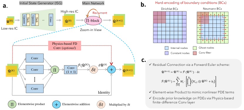
Figure 1: Schematic architecture of PeRCNN: a. the network with a $\Pi$-block for the recurrent computation; b. embedding of BCs; and c. key features of the network. Here, $\tilde{\mathbf{u}}^{(0)}$ denotes the low-res noisy measurement of the initial state, while $\widehat{\boldsymbol{\mathcal{U}}}^{(k)}$ denotes the predicted fine-res solution at time $t_{k}$. The decoder (initial state generator) is used to downscale/upsample the low-resolution initial state.

Reaction-diffusion Systems

Reaction-diffusion (RD) equations have found wide applications in the analysis of pattern formation [50], such as population dynamics [51], chemical reactions [52], cell proliferations [53], and etc. In this article, we specifically consider three different RD systems of the Lambda–Omega ($\lambda$–$\Omega$), FitzHugh-Nagumo (FN) and Gray-Scott (GS) types to verify the proposed approach. In general, the RD system can be described by the following governing equation

$$\mathbf{u}_{t}=\mathbf{D}\Delta\mathbf{u}+\mathbf{R(u)}$$ (1)

where $\mathbf{u}\in\mathbb{R}^{n}$ is the vector of concentration variables, $\mathbf{D}\in\mathbb{R}^{n\times n}$ is the diagonal diffusion coefficient matrix, $\Delta$ is the Laplacian operator, and $\mathbf{R(u)}$ is the reaction vector that represents the interactions among components of $\mathbf{u}$. Without loss of generality, let us assume the RD system features two components, i.e., $\mathbf{u}=[u,\leavevmode\nobreak\ v]^{\texttt{T}}$. Specifically, the $\lambda$–$\Omega$ RD system is governed by

$$u_{t} =\mu_{u}\Delta u+(1-u^{2}-v^{2})u+\beta(u^{2}+v^{2})v$$ (2)

$$v_{t} =\mu_{v}\Delta v-\beta(u^{2}+v^{2})u+(1-u^{2}-v^{2})v$$

while FN RD system can be described by

$$u_{t} =\mu_{u}\Delta u+u-u^{3}-v+\alpha$$ (3)

$$v_{t} =\mu_{v}\Delta v+(u-v)\beta$$

where $\alpha$ and $\beta$ are the coefficients prescribing the reaction process and take different values. Similarly, the GS RD system can be described by

$$u_{t} =\mu_{u}\Delta u-uv^{2}+F(1-u)$$ (4)

$$v_{t} =\mu_{v}\Delta v+uv^{2}-(F+\kappa)v$$

where $\kappa$ and $F$ denote the kill and feed rate, respectively. For the FN and GS RD systems, we consider both two-dimensional (2D) and three-dimensional (3D) cases in this article. To generate the numerical solution as the ground truth reference, we discretize the regular physical domain with Cartesian grid and utilize a high-order finite difference method to simulate the evolution of the RD system. The computational and discretization parameters for each case are provided in Extended Data Table 1.

Forward Analysis of PDE Systems

Solving general PDEs is undoubtedly the cornerstone of scientific computing. We herein demonstrate the capability of PeRCNN for forward analysis of PDE systems (i.e., solving PDEs), in particular, the aforementioned RD systems. It is assumed that the governing PDEs, together with the necessary initial and boundary conditions (I/BCs), of the physical system are completely known. Therefore, the prescribed initial state is fed to the network for the recurrent computation without resorting to ISG. Once the forward recurrent computation is finished, the snapshot (or prediction) at each time step is collected. The finite difference is then applied on the discrete snapshots for computing the partial derivatives involved in the governing PDE. The mean squared error (MSE) of the equation residual is used as the optimization objective (or loss function) for obtaining a set of model’s parameters. Multiple RD systems, including the 2D $\lambda$–$\Omega$, 2D/3D FN and 2D GS RD equations, are considered herein as the numerical examples. The ground truth reference solution is generated by the high-order finite difference method. The governing PDEs, computational domain and discretization settings for each system are provided in Extended Data Table 1. Detailed discussions on the network settings is given in Supplementary Note C. Details on how to properly select the spatial and temporal grid sizes, in order to ensure model’s numerical stability and achieve desired solution resolution, are given in Supplementary Note H.

Figure 2 shows the snapshots predicted by the PeRCNN for each system at a given time. To compare the performance of the proposed approach with existing methods, we also provide the result of two baseline models, namely, the Convolutional Long-Short Term Memory (ConvLSTM) [54] and Physics-informed Neural Network (PINN) [24]. It can be seen that the solution obtained by PeRCNN agrees well with the reference for all four cases. In contrast, the ConvLSTM and PINN perform differently on 2D and 3D cases; in particular, they get a fairly good prediction for 2D cases while considerably deviate from the reference for 3D cases. To examine the accuracy of each method as a PDE solver, we compute the accumulative Rooted Mean Square Error (RMSE) of the prediction. It shows that PeRCNN achieves a significantly lower error throughout the considered time-marching interval. Although existing techniques (e.g., finite difference/volume/element methods) for solving PDEs are already mature nowadays, the result in this part demonstrates the promise of PeRCNN on modeling and simulation of complex systems.

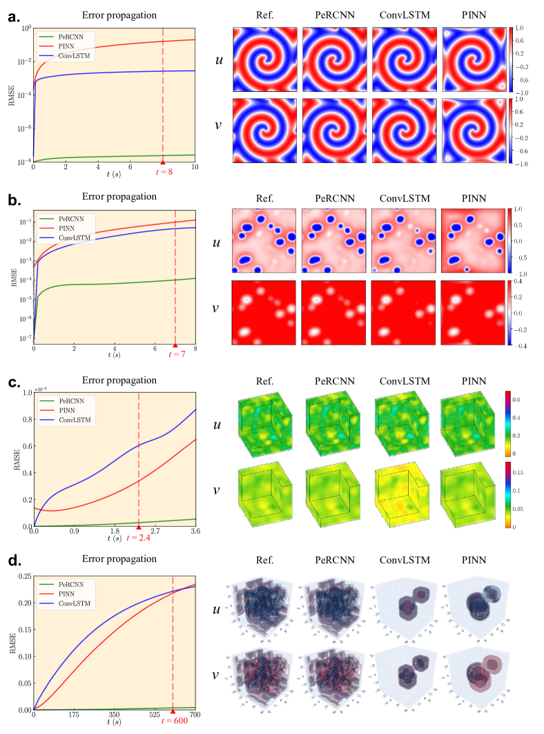
Figure 2: Error propagation curve (left) and predicted snapshots (right) by PeRCNN, ConvLSTM and PINN on various RD systems. a, 2D $\lambda$–$\Omega$ RD equation. b, 2D FN RD equation. c, 3D FN RD equation. and d, 3D GS RD equation. Note that only a corner of the solution field is shown for the FN RD systems in c for better visualization of the internal solution distribution.

Inverse Analysis of PDE Systems

Calibrating the unknown parameters of a given model against experimental data is a commonly seen problem in scientific discovery, e.g., one might be interested in uncovering the scalar coefficients in the governing PDEs given very limited observed snapshots of the system. Since the proposed PeRCNN has the capability of encoding the PDE structure (e.g., known terms) into the network architecture for predicting spatiotemporal systems, we can apply it to identify the unknown coefficients by treating them as trainable variables. To verify the effectiveness of PeRCNN in inverse analysis of PDEs, we consider the 2D GS RD system governed by the following two coupled equations: $u_{t}=\mu_{u}\Delta u-c_{1}\cdot uv^{2}+c_{F}(1-u)$ and $v_{t}=\mu_{v}\Delta v+c_{2}\cdot uv^{2}-(c_{F}+c_{\kappa})v$, where $\mu_{u}$, $\mu_{v}$, $c_{1}$, $c_{2}$, $c_{F}$ and $c_{\kappa}$ are unknown coefficients. Since the explicit form of the governing PDEs is known, we construct the physics-based FD Conv connections (i.e., diffusion and other polynomial terms) according to the RHS of the governing equation. Note that no element-wise product layer is involved in the network. In the meanwhile, each unknown coefficient is treated as an individual trainable variable in the computational graph for the forward/backward computations.

To examine the capability of the model in scenarios of various data availability, we consider two different sets of measurement data. In the first scenario (S1), the available measurement includes multiple noisy and low-resolution snapshots of the system, which means the available data is scarce spatially while somewhat abundant in the temporal dimension. In the second scenario (S2), we assume only the first and last snapshots of the system with decent resolution are available. These two scenarios reflect the trade-off between the spatial and temporal resolution of the existing measurement. These synthetic measurements accompanied with 10% Gaussian noise are shown in Figure 3a-b. The misfit error between the prediction and the measurement data is computed as the loss function for optimizing the unknowns. To prevent the overfitting to noise, early stopping is employed by splitting the dataset into training/validation sets. The details of computational parameters for dataset generation, network architecture, initialization of coefficients and optimization settings are presented in Supplementary Note D.

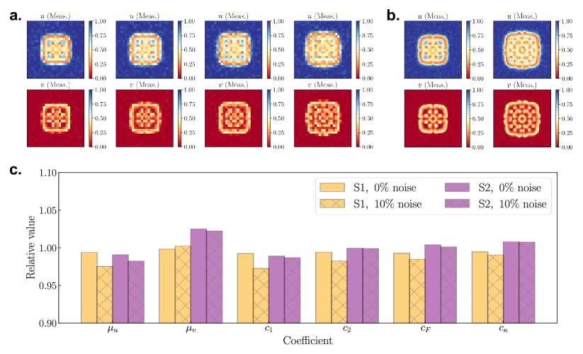
Figure 3: Snapshots of the measurement data employed in the experiment and the identified coefficients. a, Data availability in Scenario 1 (multiple snapshots with $26\times 26$ resolution). b, Data availability in Scenario 2 (initial and last snapshots with $51\times 51$ resolution). c, Identified coefficient at various noise level and data availability.

To test the effects of noise, the experiment is also performed on clean data. Each case encompasses 10 runs with various random seed for coefficient initialization. The identified coefficients are presented in Figure 3c and Extended Data Table 2. It can be seen that, in all cases, PeRCNN is able to uncover the unknown coefficients with satisfactory accuracy. Compared with the identified coefficients in the noise-free case, the result only deteriorates slightly with 10% noise. In the absence of the noise, the identified coefficients feature high accuracy, with the mean absolute relative error (MARE) for all the coefficients being 0.6%. For the case with 10% noise, the MARE is 1.61% in spite of 10% Gaussian noise in the measurement. PeRCNN also shows superiority to PINN (see the result reported in Supplementary Table S.4). Moreover, the potential of employing PeRCNN to identify space-varying coefficients is further demonstrated in Supplementary Note D.5). The numerical results in this section illustrates the good capability of our model on the inverse analysis of PDE systems.

Data-driven Modeling of Spatiotemporal Dynamics

PDEs play an an essential role in modeling physical systems. However, there still exist a considerable portion of systems, such as those in epidemiology, climate science and biology, whose underlying governing PDEs are either completely unknown or only partially known. Thanks to the ever-growing data availability as well as recent advances in scientific machine learning, data-driven modeling nowadays becomes an effective way to establish predictive models for physical systems. Since the proposed network is characterized with excellent expressiveness for representing nonlinear dynamics (see Methods: Universal Polynomial Approximation Property for $\Pi$-block) and capability of encoding incomplete governing PDE, it has great potential to serve as a generalizable and robust data-driven model for predicting high-resolution nonlinear spatiotemporal dynamics. In this part, we primarily focus on data-driven modeling of spatiotemporal dynamics by the proposed physics-encoded learning paradigm given limited, noisy measurement data.

Let us assume some low-resolution and potentially noisy snapshots of the system are measured, i.e., $\tilde{\mathbf{u}}\in\mathbb{R}^{n_{t}^{\prime}\times n\times H^{\prime}\times W^{\prime}}$ where $n_{t}^{\prime}$ is the number of snapshots, $n$ is the number of state variable components and $H^{\prime}\times W^{\prime}$ is the resolution of each snapshot. We seek to establish a predictive model that gives the most likely high-resolution solution $\boldsymbol{\widehat{\mathcal{U}}}\in\mathbb{R}^{n_{t}\times n\times H\times W}$ where $n_{t}^{\prime}<n_{t}$, $H^{\prime}<H$ and $W^{\prime}<W$, and possesses satisfactory extrapolation ability over the temporal horizon (e.g., for $t>t_{n_{t}}$). As we have seen, one salient characteristic of PeRCNN is the capability of encoding prior knowledge (e.g., the general PDE structure and/or I/BC) into the learning model. In particular, we assume the basic PDE form as shown in Eq. (4) is given, where the diffusion term is known a priori whose coefficients are however unknown. To compare PeRCNN with existing methods, we also perform experiments on several baseline models, namely, the recurrent ResNet [55, 56], ConvLSTM [54], PDE-Net [5] and deep hidden physics model (DHPM) [57]. Once the training is done, we infer the high-resolution prediction from the predictive data-driven models. The accumulative rooted-mean-square error (RMSE) and the physics residual (see Supplementary Note E.3 for definition) are utilized to evaluate the accuracy of the established data-driven models.

We verify the performance of PeRCNN using synthetic datasets of the 2D and 3D GS RD equation systems, whose computational parameters and discretization setting are provided in Extended Data Table 1. In the experiments, we fix the amount of data, training/validation/testing dataset splitting, the number of prediction steps, the Gaussian noise level (10%) and the random seed for each method. The hyperparameters for each case are selected through hold-out cross validation. The synthetic measurement data (i.e., some low-resolution snapshots) is downsampled (in both spatial and temporal dimension) from the numerical solution. Once the model is finalized, extrapolation beyond temporal horizon, e.g., for $t>t_{n_{t}}$, would be performed to examine the extrapolation ability of each model. Note that comprehensive sensitivity tests of PeRCNN in the context of some major hyperparameters (i.e., filter size, number of Conv layers and number of channels) are presented in Supplementary Note E.4.

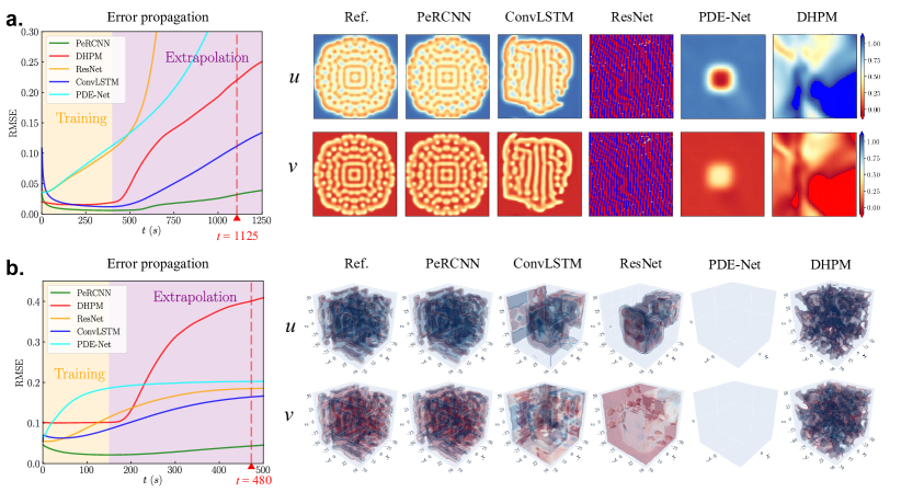
Figure 4: Error propagation curve of the prediction (left) and the extrapolated snapshots (right) from each data-driven model compared with the reference solution. Note that extrapolation is performed beyond the time horizon of the measurement data while the time of each snapshot is marked by a dash red line in the error propagation curve. a, 2D GS RD equation. b, 3D GS RD equation.

2D Gray-Scott RD equation.

In this case, we consider a data availability scenario where the resolution of measurement data is relatively low in space but decent in time. The available measurement data in this case encompasses 41 noisy snapshots of on a $26\times 26$ grid, ranging from $t=0$ to $400$ s. Since we assume the dynamical system of interest features the ubiquitous diffusion phenomenon, the governing PDE (i.e., $\mathcal{F}$) is known to have a diffusion term ($\Delta\mathbf{u}$) whose scalar coefficients are still unknown. Therefore, we encode the diffusion term into PeRCNN by creating a physics-based FD Conv connection with the discrete Laplace operator as the Conv kernel (see Supplementary Note B.3). Furthermore, the diffusion coefficient ($\tilde{\mu}$) is first estimated by solving a linear regression problem of $u_{t}=\tilde{\mu}\Delta u$ with the available data. Then a lower bound of $0$ and upper-bound of $2\tilde{\mu}$ are applied to ensure the stability of diffusion. Each model is responsible for predicting 801 fine-resolution snapshots during the training phase, while 1700 extra snapshots are predicted for extrapolation.

Snapshots at different time instants are presented in Figure 4a, which reveal the complex maze-like pattern of the GS-RD system. We report that the recurrent ResNet and PDE-Net are unable to reconstruct the fine-resolution snapshots even in the training due to the limited noisy training data, after trying all the hyperparameter combinations within a range (see Supplementary Note E.5.1). Apart from that, it can be seen from the snapshots that PeRCNN is the only model working well for long-time extrapolation in spite of minor discrepancies. It is also interesting to note that PeRCNN with filter size of 1 works as good as the model with larger filters (e.g., 3 or 5). This is because the reaction term of the GS-RD system contains no spatial derivatives, making the $1\times 1$ filter sufficient for representing the nonlinear reaction terms. This implies that prior knowledge on the governing PDE can also be employed while designing the data-driven model. To quantitatively measure the extrapolation capability of our model, we also plot the evolution of accumulative RMSE in Figure 4a. It is observed that PeRCNN outperforms the competitors at all stages in the context of error propagation, which further confirms the extrapolation ability of PeRCNN. We may notice that the accumulative RMSE starts from an initial high value. This is due to the fact that the training data is corrupted by 10% Gaussian noise and the metric is computed from one single snapshot at the beginning. The effect of the unrelated noise gradually fades out as more time steps are considered.

3D Gray-Scott RD equation.

In this example, we test our method on the 3D GS RD system. As the computational intensity of this higher dimensional example brings challenges to the existing methods, we aim to scrutinize the performance of our PeRCNN regarding the scalability and computational efficiency. The training data used to establish the data-driven model includes 21 noisy low-resolution snapshots ($25^{3}$) uniformly sampled from $t=0$ to $150$ s. The prior knowledge on the system and the estimation of the diffusion coefficients as discussed in the previous 2D GS RD example are adopted here as well. Each trained model produces 301 high-resolution ($49^{3}$) snapshots during the learning stage, while 700 extrapolation steps are predicted once each model is finalized. The predicted isosurfaces of two levels are plotted in Figure 4b. It should be noted that the plot of PDE-Net is blank because the prediction range falls out of the two selected isosurface levels. Similar to the previous case, we observe that PeRCNN is the only model that gives a satisfactory long-term prediction. The flat error propagation curve of PeRCNN, as shown in Figure 4b, also demonstrates the remarkable generalization capability of PeRCNN.

In Supplementary Note E.5, we compare the number of trainable parameters, the training time per epoch, and the RMSE of both training and extrapolation for each model. It is found that PeRCNN is characterized with good model efficiency as it uses the least amount of training parameters. For the 3D case where the training efficiency of the network is of great concern, the elapsed time for training one epoch by PeRCNN is comparable to that of the ResNet, which is widely acknowledged to be an efficient network architecture. As for the accuracy of the training and extrapolation, our model outperforms the baselines consistently across different examples. In a nutshell, PeRCNN outperforms the other three baselines with many fewer trainable parameters and higher accuracy.

Generalization to Different ICs.

It is evident that the trained model has good extrapolation capability along the time horizon. Here, we further explore how the trained model generalizes to different initial conditions (ICs). To set up the experiment, we employ the above trained model to perform inference with a different IC. It should be noted that the baseline DHPM is ineligible for inference with different ICs as it is based on FCNN. The prediction result is depicted in Figure 5. It is seen that PeRCNN gives consistent prediction compared with the ground truth reference solution. On the contrary, the considered baseline models (e.g., recurrent ResNet, ConvLSTM and PDE-Net) are unable to generalize to an unseen IC. They give wild prediction because of their incapability of learning the underlying physics (e.g., caused by the black-box property of the model). In addition, the error propagation of the prediction in Figure 5 indicates clearly the excellent generalization capability of the proposed model. In the later subsection of Interpretability of the Learned Model, we show the extracted expression from the trained PeRCNN model is very close to the genuine $\mathcal{F}$, which to a large degree explains the remarkable generalization capability of our model given the fact that the trained PeRCNN model parameterizes the spatiotemporal dynamics well.

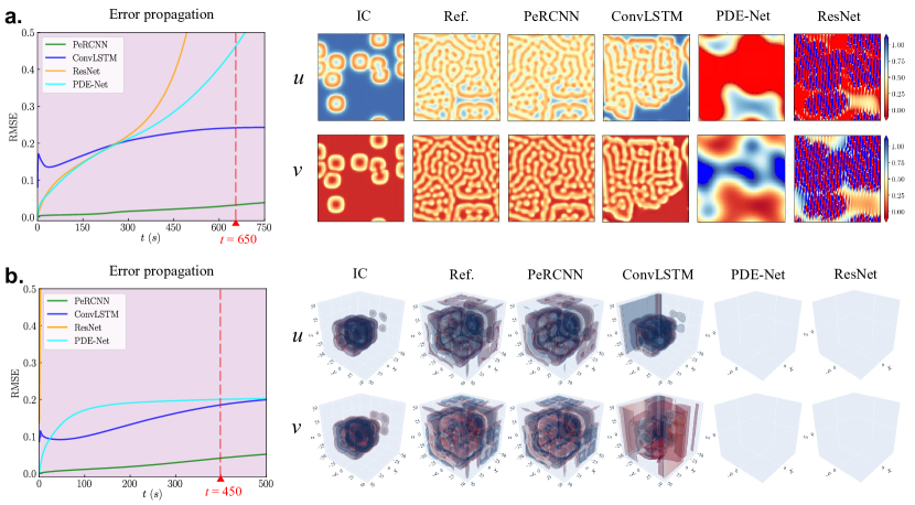
Figure 5: Error propagation curve (left) and the snapshots (right) of the inference result. The results are obtained by performing inference on the data-driven model from subsection Data-driven Modeling using a different initial condition. a, 2D GS RD equation. b, 3D GS RD equation.

Data-driven Discovery of PDEs with Scarce and Noisy Data

In previous sections, we primarily investigate the scientific modeling tasks (e.g., forward simulation or data-driven modeling) using the proposed model, which exhibits excellent accuracy and extrapolation ability as identified from the numerical results. However, the process of knowledge discovery does not end at modeling the physical phenomena of interests. More importantly, it is the translation of the learned patterns from the data (e.g., formulated PDEs or empirical relationships) that lead scientists to understand the cause-effect relationship among physical variables, and further make inference on similar problems. Therefore, in this section, we extend the proposed physics-encoded learning model for discovering the closed-form governing PDEs [58]. To formulate this problem, let us again consider the nonlinear system described by Eq. (7). The objective of the equation discovery is to recover the closed form of the governing PDEs given the scarce and noisy measurement of the system. To this end, we integrate the sparse regression technique [15] with our PeRCNN model for solving this problem. The proposed framework for the PDE discovery is presented in Figure 6 with the example of 2D GS-RD equation. The entire procedure consists of three steps, including data reconstruction (Figure 6a), sparse regression (Figure 6b) and coefficients fine tuning (Figure 6c), as discussed in Methods: Equation Discovery.

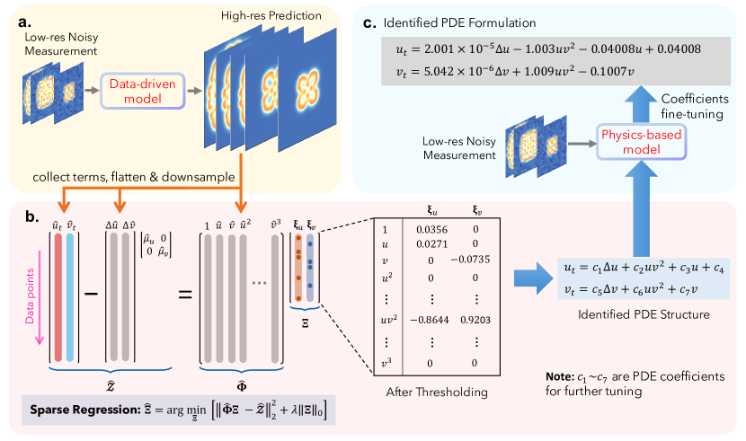
Figure 6: Flowchart of the discovery of governing PDEs. a. data reconstruction: data-driven model constructed from low-res and noisy measurement is used to generate high-res prediction for sparse regression; b. sparse regression: STRidge algorithm is used to obtain the sparse coefficient matrix $\boldsymbol{\Xi}$; c. coefficients fine-tuning: the PeRCNN built based on identified PDE structure is employed to fine-tune the coefficient from the sparse regression.

To validate the effectiveness of the our method, we perform the equation discovery on two RD systems (e.g., 2D GS and $\lambda$–$\Omega$ RD systems) using synthetic datasets, which are obtained by downsampling the noise-corrupted numerical solution. Two different Gaussian noise levels (5% and 10%), as well as the noise-free case, are considered in the experiment. As we assume the ubiquitous diffusion phenomenon exists in the concerned system, a shortcut diffusion Conv layer is encoded into the network for data reconstruction (see Figure 1a). Accordingly, the coefficients corresponding to $\Delta(\mathbf{u})$ are exempted from being filtered in the STRidge algorithm. Once the equation discovery is finished, we measure the performance of the proposed method using the metrics of precision, recall and relative $\ell_{2}$ error of the coefficient vector. Technical details of the generation of synthetic measurement data and the evaluation metrics can be found in Supplementary Note F.3.

The discovered PDEs by our method are provided in Extended Data Table 3. It is seen that our method is able to recover the governing PDEs completely when the measurement data is clean or mildly polluted by noise. Even though the noise level grows to 10%, our approach still exhibits competitive performance, i.e., it uncovers the majority of terms in the PDEs. Empirical study in Supplementary Note F.5 shows that our method could handle even a much larger noise level, i.e., 30% Gaussian noise. In Supplementary Note F.4, we also compare our approach with some existing methods (or baselines) for governing PDE discovery, including PDE-FIND [16], sparse regression coupled with fully-connected neural network (FCNN) or PDE-Net [5]. The comparison shows that our approach outperforms (if not perform as good as) the considered baselines consistently under different noise levels and data richness. Visualizing the reconstructed high-fidelity data from each method (see Supplementary Figure S.17), we observe that our method has a much smaller reconstruction error as a result of fully utilizing the prior physics knowledge and the powerful expressiveness of the model. This would give rise to more accurate derivative terms in the linear system, facilitating the discovery of the governing PDEs. In summary, the effectiveness of the proposed approach is demonstrated for solving the data-driven equation discovery problem, especially when the measurement data is characterized with poor resolution and noise.

Interpretability of the Learned Model

Compared with the traditional deep neural networks, which are usually considered to be “black-box”, the proposed network architecture is designed to possess good interpretability. As each channel of the input for $\Pi$-block (i.e., $\widehat{\boldsymbol{\mathcal{U}}}^{(k)}$) corresponds to a solution component (i.e., $u$ and $v$), the multiplicative form of $\Pi$-block (see Eq. (8)) makes it possible to extract an explicit form of learned $\mathcal{F}$ from the learned weights and biases via symbolic computations. This section is dedicated to the discussion on how the learned model can be interpreted as an analytical expression, which is useful for people to understand the underlying cause-effect relationships among physical variables.

To demonstrate how to interpret the learned model, we first use the learned model from 3D GS RD case in Data-driven Modeling as an example. In this case, the parallel Conv layers in $\Pi$-block have the filter size of 1, which implies that each output channel is the linear combination of $u$, $v$ and a constant. With the element-wise product operation among three Conv layers, a third degree polynomial will be produced to account for the reaction term of the system. With the help of the SymPy [59] – a symbolic computation Python package, we can extract the learned reaction term:

In the meanwhile, the identified diffusion term can be also extracted from the trainable variables in diffusion connections, which reads $\mathbf{D(u)}=\begin{bmatrix}0.18\Delta u,\leavevmode\nobreak\ 0.08\Delta v\end{bmatrix}^{\text{T}}$. Comparing the extracted term with the ground truth PDEs, we observe some distracting terms due to the 10% noise in the training data and the redundancy of the network. Further pruning on the raw expression can be done to make it more parsimonious.

The above example is a special case where the Conv layer in $\Pi$-block has filter size of 1, which indicates no spatial derivatives are involved in reaction terms. However, we can extend the network architecture design to make it applicable to general cases. To interpret terms involving partial derivatives (e.g., $u\Delta u$, $uu_{x}$), we could completely freeze or impose moment matrix constraints on part of the convolutional filters [5]. Here, an experiment is conducted on the 2D Burgers’ equation, which has wide applications in applied mathematics such as fluid/traffic flow modeling, given by $\mathbf{u}_{t}+\mathbf{u}\cdot\nabla\mathbf{u}=\nu\Delta\mathbf{u}$, where $\mathbf{u}=[u,\leavevmode\nobreak\ v]^{\texttt{T}}$ denotes the fluid velocities and $\nu$ is the viscosity coefficient. The network employed in the experiment has two Conv layers with two channels. The first Conv layer are associated with derivative operators $\partial(\cdot)/\partial x$ and $\partial(\cdot)/\partial y$ respectively, by fixing the filters with corresponding FD stencils. The synthetic dataset is generated on $101\times 101$ Cartesian grid using high-order FD method with $\nu=0.005$. The noise-free synthetic measurement data used for constructing the model includes 11 low-resolution ($51\times 51$) snapshots uniformly selected from the time period of $t\in[0,\leavevmode\nobreak\ 0.1]$.

After the model is trained, we interpret the expression from the PeRCNN model, which reads:

It can be observed that the equivalent expression of the learned model matches well the genuine governing PDEs, except some minor terms whose coefficients are close to zero. In addition, the extracted expression helps explain the extraordinary extrapolation and generalization capabilities of our model. Although the selection of differential operators to be embedded is crucial for identifying the genuine form of the $\mathcal{F}$, the above two examples demonstrate the interpretability of PeRCNN over common “black-box” models.

DISCUSSION

This paper introduces a novel deep learning architecture, namely PeRCNN, for modeling and discovery of nonlinear spatiotemporal dynamical systems based on sparse and noisy data. One major advantage of PeRCNN is that the prior physics knowledge can be encoded into the network, which guarantees the resulting network strictly obeys given physics (e.g., initial and boundary conditions, general PDE structure, and known terms in PDEs). This brings distinct benefits for improving the convergence of training and accuracy of the model. Through extensive numerical experiments, we show the efficacy of PeRCNN for forward and inverse analysis of reaction-diffusion type PDEs. The comparison with several baseline models demonstrates that the proposed physics-encoded learning paradigm uniquely possesses remarkable extrapolation ability, generalizability and robustness against data noise/scarcity. Although we demonstrate the effectiveness of the PeRCNN on various reaction-diffusion systems, the model is in theory applicable to other types of spatiotemporal PDEs (e.g., the 2D Burgers’ equation with the convection term shown in Supplementary Note F.4, and the Kolmogorov turbulent flows at Reynolds number = 1,000 discussed in Supplementary Note J).

Equally important, PeRCNN shows good interpretability due to the multiplicative form of the $\Pi$-block. An analytical expression that governs the underlying physics can be further extracted from the learned model via symbolic computation. In particular, we successfully marry PeRCNN to the sparse regression algorithm to solve the crucial PDE discovery issues. The coupled scheme enables us to iteratively optimize the network parameters, and fine-tune the discovered PDE structures and coefficients, essentially leading to the final parsimonious closed-form PDEs. The resulting framework will serve as an effective, interpretable and flexible approach to accurately and reliably discover the underlying physical laws from imperfect and coarse-meshed measurements.

Although PeRCNN shows promise in data-driven modeling of complex systems, it is restricted by the computational bottleneck due to the high dimensionality of the discretized system, especially when it comes to systems in a large 3D spatial domain with long-term evolution. However, this issue is expected to be addressed via temporal batch and multi-GPU training. In addition, the current model is rooted in standard convolution operations, which limits its applicability to irregular meshes of arbitrary computational geometries. This issue might be resolved by introducing graph convolution into the network architecture. Lastly, since the PeRCNN network is designed based on the assumption that the underlying governing PDEs have a polynomial form (very commonly seen in standard PDEs for modeling of physics such as diffusion, reaction, convection, and rotation), it might be less capable or too redundant (if many channels are used to achieve a high polynomial degree) of modeling unique spatiotemporal dynamics whose governing PDEs are parsimonious but involves other advanced symbolic operators such as division, sin, cos, exp, tan, sinh, log, etc. Although PeRCNN shows success in data-driven modeling of a PDE system with non-polynomial term in Supplementary Note I, how to design a network that properly incorporates a limited number of mathematical operators as symbolic activation functions to improve the representation ability still remains an open question. We aim to systematically address these issues in our future study.

METHODS

We herein introduce the method of the proposed PeRCNN model. More details can be found in Supplementary Note B.

Network Architecture

Let us first consider a spatiotemporal dynamical system described by a set of nonlinear, coupled PDEs as

$$\mathbf{u}_{t}=\mathcal{F}\left(\mathbf{x},t,\mathbf{u},\mathbf{u}^{2},\nabla_{\mathbf{x}}\mathbf{u},\mathbf{u}\cdot\nabla_{\mathbf{x}}\mathbf{u},\nabla^{2}\mathbf{u},\cdots\right)$$ (7)

where $\mathbf{u}(\mathbf{x},t)\in\mathbb{R}^{n}$ denotes the state variable with $n$ components defined over the spatiotemporal domain $\{(\mathbf{x},t)\}\in\Omega\times\mathcal{T}$. Here, $\Omega$ and $\mathcal{T}$ represent the spatial and temporal domain, respectively; $\nabla_{\mathbf{x}}$ is the Nabla operator with respect to the spatial coordinate $\mathbf{x}$; and $\mathcal{F}(\cdot)$ is a nonlinear function describing the right hand side (RHS) of PDEs. The solution to this problem is subject to the initial condition (IC) $\mathcal{I}(\mathbf{u};t=0,\mathbf{x}\in\Omega)=0$ and the boundary condition (BC) $\mathcal{B}(\mathbf{u},\nabla_{\mathbf{x}}\mathbf{u},\cdots;\mathbf{x}\in\partial\Omega)=0$. Since we mainly focus on regular physical domains in this paper, state variable $\mathbf{u}$ are defined on a discretized Cartesian grid.

Borrowing the concepts of numerical discretization, we build the physics-encoded spatiotemporal learning model on the basis of a forward Euler scheme. That said, the state variable $\mathbf{u}$ would be updated by a recurrent network given by $\widehat{\mathbf{u}}^{(k+1)}=\widehat{\mathbf{u}}^{(k)}+\widehat{\mathcal{F}}(\widehat{\mathbf{u}}^{(k)};\boldsymbol{\theta})\delta t$, where $\delta t$ is the time spacing, $\widehat{\mathbf{u}}^{(k)}$ is the prediction at time $t_{k}$ and $\widehat{\mathcal{F}}$ is the approximated $\mathcal{F}$ parameterized by $\boldsymbol{\theta}$ that ensembles a series of operations for computing the RHS of Eq. (7). Similar ideas of applying numerical discretization (e.g., backward Euler or Runge-Kutta) to designing deep learning architectures can be found in some recent literature [60, 61, 5, 62, 63, 64].

Following the above intuition, here we introduce the proposed network, namely the Physics-encoded Recurrent Convolutional Neural Network (PeRCNN). The architecture of this network (as shown in Figure 1) consists of two major components: a fully convolutional (Conv) network as initial state generator (ISG) and an novel Conv block called $\Pi$-block (product) used for recurrent computation. ISG is introduced to produce the high-resolution initial state $\widehat{\boldsymbol{\mathcal{U}}}^{(0)}$ in the case that only low-resolution initial state (or measurement) $\tilde{\mathbf{u}}^{(0)}$ is available as initial condition. Note that $\tilde{\mathbf{u}}$ is used to denote the low-resolution snapshots (or measurement) while the superscript “0” indicates the first one. Similarly, $\widehat{\boldsymbol{\mathcal{U}}}$ is used to represent the high-resolution prediction from the model. Within the $\Pi$-block, the core of PeRCNN, the state variable $\widehat{\boldsymbol{\mathcal{U}}}^{(k)}$ from the previous time step goes through multiple parallel Conv layers. The feature maps produced by these layers are then fused through an elementwise product layer. The $1\times 1$ Conv layer is subsequently used to linearly combine multiple channels into the desired output (i.e., approximated $\mathcal{F}$). Mathematically, the $\Pi$-block seeks to approximate the function $\mathcal{F}$ via polynomial combination of solution $\widehat{\boldsymbol{\mathcal{U}}}^{(k)}$ and its spatial derivatives, given by

$$\widehat{\mathcal{F}}\left(\widehat{\boldsymbol{\mathcal{U}}}^{(k)}\right)=\sum_{c=1}^{N_{c}}W_{c}\cdot\left[\prod_{l=1}^{N_{l}}\left(\mathcal{K}_{c,l}\circledast\widehat{\boldsymbol{\mathcal{U}}}^{(k)}+b_{l}\right)\right]$$ (8)

where $N_{c}$ and $N_{l}$ are the numbers of channels and parallel Conv layers respectively; $\circledast$ denotes the Conv operation; $\mathcal{K}_{c,l}$ denotes the weight of Conv filter of $l$-th layer and $c$-th channel, while $b_{l}$ represents the bias of $l$-th layer; $W_{c}$ is the weight corresponding to $c$-th channel in $1\times 1$ Conv layer while the bias is omitted for simplicity. This multiplicative representation promotes the network expressiveness for nonlinear functions $\mathcal{F}$, compared with the additive representation commonly seen in related work [5, 65]. For detailed discussion on the design of $\Pi$-block, please refer to Supplementary Note B.

Due to the discretized scheme of the learning model, it is possible to encode prior physics knowledge of the system into network architecture, which contributes to a well-posed optimization problem. Given some existing terms in the PDE, we could encode these terms into the network by creating a shortcut connection, namely the physics-based finite difference (FD) Conv connection, from $\widehat{\boldsymbol{\mathcal{U}}}^{(k)}$ to $\widehat{\boldsymbol{\mathcal{U}}}^{(k+1)}$ as shown in Figure 1. The convolutional kernel in this physics-based Conv layer would be fixed with the corresponding FD stencil to account for the known terms. A major advantage of this encoding mechanism over the soft penalty in physics-informed learning models is the capability to leverage the incomplete PDE in the learning. In the numerical examples, we demonstrate that such a highway connection could accelerate the training speed and improve the model inference accuracy significantly. In a nutshell, the physics-based Conv connection is built to account for the known physics, while the $\Pi$-block is designed to learn the complementary unknown dynamics.

In addition to the incomplete PDE, the boundary conditions (e.g., Dirichlet or Neumann type) can also be encoded into the learning model. Inspired by the idea from the FD method, we apply the physics-based padding to the model’s prediction at each time step, as shown by Figure 1b. Specifically, for the Dirichlet BCs, we pad the prediction with prescribed values. Likewise, the padding value of Neumann or Robin BCs will be computed based on the boundary values and the gradient information. A comprehensive discussion on the padding mechanism for various BCs (e.g., Dirichlet, Neumann, Robin and Periodic) can be found in Supplementary Note B.3. In particular, we show the effectiveness of the proposed padding method in Supplementary Note G, where the Neumann BCs are considered for example.

Motivation of the Network Architecture Design

In the subsection of Physics-encoded Spatiotemporal Learning, we have introduced the proposed network architecture for learning spatiotemporal dynamical systems. Here a further discussion on the design philosophy is presented to showcase the primary motivations. A distinct characteristic of this architecture is the usage of $\Pi$-block as a universal polynomial approximator to nonlinear functions, instead of utilizing a sequence of linear layers intertwined with nonlinear activation layers commonly seen in traditional deep networks. The motivations for introducing the elementwise product operation in $\Pi$-block are three-fold:

• Though the nonlinear activation function is crucial to the universal approximation property of the deep neural network (DNN), it is also a source of poor interpretability. For example, the conventional DNN would form a prolonged nested function that is usually intractable to humans. We consider it unfavorable to use these nonlinear functions to build a recurrent block that aims to generalize the unknown physics.

• The elementwise product operation makes a better approximation to $\mathcal{F}$ in the form of multivariate polynomial (e.g., $\mathbf{u}\cdot\nabla u+u^{2}v$), which covers a wide range of well-known dynamical systems, such as Navier-Stokes, reaction-diffusion (RD), Lorenz, Schr$\ddot{\text{o}}$dinger equations, to name only a few. Since the spatial derivatives can be computed by Conv filters [66], a $\Pi$-block with $n$ parallel Conv layers of appropriate filter size is able to represent a polynomial up to the $n^{\text{th}}$ order.

• Compared with the regression models (e.g., linear or symbolic regression) relying on predefined basis functions or prior knowledge (e.g., the highest order) on $\mathcal{F}$ [15, 5], the $\Pi$-block is flexible at generalizing the nonlinear function $\mathcal{F}$. For example, a $\Pi$-block with 2 parallel layers of appropriate filter size ensembles a family of polynomials up to the 2${}^{\text{nd}}$ order (e.g., $u$, $\Delta u$, $uv$, $\mathbf{u}\cdot\nabla u$), with no need to explicitly define the basis.

Since the network architecture roots on numerical discretization, nice mathematical properties (see the next subsection) exist to guarantee the universal polynomial approximation property of $\Pi$-block. In addition, the flexibility to deal with a variety of problems in scientific modeling is another advantage possessed by the proposed network architecture. The $\Pi$-block acts as a universal polynomial approximator to unknown nonlinear function while the physics-based Conv layer accounts for the prior knowledge on the governing equation. Such a way of encoding the prior physics knowledge into the network architecture could effectively narrow down the space of feasible model parameters, hence leading to the reduced training effort required (e.g. memory, FLOPs, etc.). Furthermore, in many prediction tasks involving nonlinear system, a mixture of partial physics knowledge and scarce amount of measurement data of the system is available, which is when the proposed PeRCNN has a huge advantage over the traditional deep network. As shown in the subsection of Data-driven Modeling, we demonstrated the capability of proposed PeRCNN at handling the modeling tasks given limited physics knowledge and some low-resolution snapshots of the system. An extreme case is when the analytical form of a physical system is completely known except some scalar coefficients. The physics-based Conv layers associated with trainable variables can be created to exactly express the physical system up to discretization error. In such a case, the PeRCNN can be assumed to recover to FD method with some trainable variables. In the subsection of Inverse Analysis of PDE Systems, we showed how the proposed PeRCNN can be applied to identify the system coefficients from the noisy and scarce data in such a scenario.

Noteworthy, we mainly consider the nonlinear function $\mathcal{F}$ in the form of polynomial which is very commonly seen in PDEs. Other terms such as trigonometric and exponential functions are not considered in this work for simplicity. However, incorporating them would require no more effort than adding a particular symbolic activation (e.g., sin, cos, exp, etc.) layer following the Conv operation. What’s more, these functions can be approximated by polynomials based on Taylor series as argued in [15].

Universal Polynomial Approximation Property for $\Pi$-block

In the proposed PeRCNN, $\Pi$-block acts as an universal polynomial approximator to unknown nonlinear functions while the physics-based FD Conv layer (i.e., with FD stencil as the Conv filter) accounts for the prior knowledge on the governing equation. Notably, the $\Pi$-block achieves its nonlinearity through the element-wise product operation (see Eq. (8)) which renders the network better expressiveness compared with the additive form representation $\widehat{\mathcal{F}}(\mathbf{u})=\sum_{1\leq i\leq N}f_{i}\cdot\left(\mathcal{K}_{i}\circledast\mathbf{u}\right)$ seen in related work [5, 65] where $N$ is the number of Conv layer, $\mathcal{K}_{i}$ is the Conv kernel of $i$th layer and $f_{i}$ is the weight of $i$th layer’s output. To support this claim, we propose the following theorem and Lemmas to prove that any dynamical system described by Eq. (7) whose $\mathcal{F}$ is continuous (e.g., preferably in the form of polynomial) can be approximated by the proposed network. Without loss of generality, we consider the state variable $\mathbf{u}$ with one components $u$. Lemma 1 and Lemma 2 guarantee the accuracy of the approximation of $\widehat{\mathcal{F}}$ (see Eq. (8)) and the forward computation $\widehat{u}^{(k+1)}=\widehat{u}^{(k)}+\widehat{\mathcal{F}}(\widehat{u}^{(k)};\boldsymbol{\theta})\delta t$ respectively.

Lemma 1: Trainable convolutional filter $\mathcal{K}$ can approximate any differential operator with prescribed order of accuracy.

Proof: Consider a bivariate differential operator $\mathcal{L}(\cdot)$, we have (reproduced from [20]):

$$\mathcal{L}(u) =\sum_{k_{1},k_{2}=-\frac{p-1}{2}}^{\frac{p-1}{2}}\mathcal{K}[k_{1},k_{2}]\sum_{i,j=0}^{p-1}\frac{\partial^{i+j}u}{\partial^{i}x\partial^{j}y}\bigg{|}_{(x,y)}\frac{k_{1}^{i}k_{2}^{j}}{i!j!}\delta x^{i}\delta y^{j}+\mathcal{O}(|\delta x|^{p-1}+|\delta y|^{p-1})$$ (9)

$$=\sum_{k_{1},k_{2}=-\frac{p-1}{2}}^{\frac{p-1}{2}}\mathcal{K}[k_{1},k_{2}]u(x+k_{1}\delta x,y+k_{2}\delta y)+\mathcal{O}(|\delta x|^{p-1}+|\delta y|^{p-1})$$

$$=\mathcal{K}\circledast u+\mathcal{O}(|\delta x|^{p-1}+|\delta y|^{p-1})$$

where $p$ is the size of the filter indexed by $k_{1}$ and $k_{2}$. Letting the filter’s entry $\mathcal{K}[k_{1},k_{2}]$ be the corresponding Taylor series coefficient, we can see the error of approximation is bounded by $\mathcal{O}(|\delta x|^{p-1}+|\delta y|^{p-1})$.

Lemma 2: Local truncation error of the forward computation (i.e., $\widehat{u}^{(k+1)}=\widehat{u}^{(k)}+\widehat{\mathcal{F}}(\widehat{u}^{(k)};\boldsymbol{\theta})\delta t$) diminishes as $\delta t$ decreases.

Proof: With the Taylor expansion of $u^{(k+1)}=u^{(k)}+\mathcal{F}(u^{(k)})\delta t+\mathcal{O}(\delta t^{2})$, we can see the truncation error of the forward computation converges to zero as $\delta t$ decreases.

Theorem 1: Suppose $\mathcal{F}:\mathbb{R}^{s}\rightarrow\mathbb{R}$ is a continuous real-valued function of multidimensional variables $\boldsymbol{\eta}\in\mathbb{R}^{s}$, where $\boldsymbol{\eta}$ denotes the set of system state $\mathbf{u}$ and its derivative terms, consisting of $s$ elements in total. For any small positive number $\epsilon$, there exist positive integers $M$ and $N$, real numbers $w_{j}$, $\gamma_{ij}$ and $b_{j}$ ($i=1,2,...,N$ and $j=1,2,...,M$), and variable set $\mathbf{E}\in\mathbb{R}^{N\times M}$, such that:

$$\left|\mathcal{F}(\boldsymbol{\eta})-\sum_{j=1}^{M}w_{j}\cdot\left[\prod_{i=1}^{N}\Big{(}\gamma_{ij}E_{ij}+b_{i}\Big{)}\right]\right|<\epsilon$$ (10)

Proof: Let us firstly denote the set of system state $\mathbf{u}$ and its derivative terms, consisting of $s$ elements in total, as $\boldsymbol{\eta}=[\mathbf{u},\mathcal{L}_{1}(\mathbf{u}),\mathcal{L}_{2}(\mathbf{u}),...,\mathcal{L}_{s-1}(\mathbf{u})]^{\texttt{T}}\in\mathbb{R}^{s}$. For example, $\boldsymbol{\eta}=[u,v,u_{x},v_{y},...]^{\texttt{T}}$. The RHS of PDEs in Eq. (7) can then be represented by $\mathcal{F}(\boldsymbol{\eta})$. Based on the multivariate Taylor’s theorem, for any small positive number $\epsilon$, there is a real-valued polynomial function $\mathcal{T}$ such that

$$\left|\mathcal{F}(\boldsymbol{\eta})-\mathcal{T}(\boldsymbol{\eta})\right|<\epsilon$$ (11)

Here, $\mathcal{T}(\boldsymbol{\eta})$ can be expressed as:

$$\mathcal{T}(\boldsymbol{\eta})=\sum_{n_{1}=0}^{n}\sum_{n_{2}=0}^{n}\cdots\sum_{n_{s}=0}^{n}\mathcal{N}(\boldsymbol{\eta})$$ (12)

where

$$\mathcal{N}(\boldsymbol{\eta})=c_{n_{1}}c_{n_{2}}\cdots c_{n_{s}}\big{(}\eta_{1}-\bar{b}_{1}\big{)}^{n_{1}}\big{(}\eta_{2}-\bar{b}_{2}\big{)}^{n_{2}}\cdots\big{(}\eta_{s}-\bar{b}_{s}\big{)}^{n_{s}}$$ (13)

Here, $c$’s denote the real-valued coefficients, $\bar{b}$’s the biases, and $n$ the maximum polynomial order. For simplicity, we omit the subscripts $\{n_{1},...,n_{s}\}$ in $\mathcal{N}(\boldsymbol{\eta})$.

Lemma 3: For real numbers $\eta$, $b$ and $c$, and integer $n^{\prime}$, there exist real-valued vector $\boldsymbol{\alpha}\in\mathbb{R}^{n+1}$, real number $\tilde{b}$ and integer $n^{\prime}\leq n$ such that $c(\eta-b)^{n^{\prime}}=\prod_{i=0}^{n}\big{(}\alpha_{i}\eta-\tilde{b}\big{)}$ if $\|\boldsymbol{\alpha}\|_{0}=n^{\prime}$.

Based on Lemma 3, there are real numbers $\alpha$’s and $\tilde{b}$’s such that $\mathcal{N}(\boldsymbol{\eta})$ can be re-written as:

$$\mathcal{N}(\boldsymbol{\eta})=\prod_{i=0}^{n}\left[\big{(}\alpha_{i1}\eta_{1}-\tilde{b}_{1}\big{)}\big{(}\alpha_{i2}\eta_{2}-\tilde{b}_{2}\big{)}\cdots\big{(}\alpha_{is}\eta_{s}-\tilde{b}_{s}\big{)}\right]\leavevmode\nobreak\ \leavevmode\nobreak\ \leavevmode\nobreak\ \text{s.t.}\leavevmode\nobreak\ \leavevmode\nobreak\ \leavevmode\nobreak\ \|\boldsymbol{\alpha}_{k}\|_{0}=n_{k}$$ (14)

where $\boldsymbol{\alpha}_{k}=[\alpha_{0k},\alpha_{1k},...,\alpha_{nk}]^{\texttt{T}}\in\mathbb{R}^{n+1}$ is the $k$-th vector of $\alpha$’s ($k=0,1,...,s$); $\|\cdot\|_{0}$ denotes the $\ell_{0}$ norm of a vector. By defining proper weights ($\boldsymbol{\beta}\in\mathbb{R}^{(n+1)s}$) and biases ($\hat{\mathbf{b}}\in\mathbb{R}^{(n+1)s}$), we can further express $\mathcal{N}(\boldsymbol{\eta})$ by:

$$\mathcal{N}(\boldsymbol{\eta})=\prod_{i=1}^{(n+1)s}\left[\beta_{i}\hat{\eta}_{i}+\hat{b}_{i}\right]$$ (15)

where $\hat{\boldsymbol{\eta}}:=\boldsymbol{\ell}\otimes\boldsymbol{\eta}\in\mathbb{R}^{(n+1)s}$ is the Kronecker transformation of $\boldsymbol{\eta}$; $\boldsymbol{\ell}\in\mathbb{R}^{n+1}$ is a column vector with all elements equal to 1; $\otimes$ denotes the Kronecker product. Note that $\boldsymbol{\beta}$ is sparse. Substituting Eq. (15) into Eq. (12), we obtain the equivalent formulation for $\mathcal{T}(\boldsymbol{\eta})$ as follows:

$$\mathcal{T}(\boldsymbol{\eta})=\sum_{j=1}^{M}w_{j}\cdot\left[\prod_{i=1}^{N}\Big{(}\gamma_{ij}E_{ij}+b_{i}\Big{)}\right]$$ (16)

where $\mathbf{E}:=\tilde{\boldsymbol{\ell}}\otimes\hat{\boldsymbol{\eta}}\in\mathbb{R}^{N\times M}$ is the Kronecker transformation of $\hat{\mathbf{E}}$; $\tilde{\boldsymbol{\ell}}\in\mathbb{R}^{M}$ is a row vector with all elements equal to 1; $\mathbf{w}\in\mathbb{R}^{M}$ and $\boldsymbol{\gamma}\in\mathbb{R}^{N\times M}$ denote some properly defined real-valued coefficients; $\mathbf{b}\in\mathbb{R}^{N}$ is the bias vector. Note that the formulation of Eq. (16) can be guaranteed when $M\geq(n+1)^{s}$ and $N\geq(n+1)s$. Substituting Eq. (16) into Eq. (11) can thus prove Theorem 1.

It is noted that the term $\gamma_{ij}E_{ij}$ in Eq. (16) can be approximated by a series convolutional filters as shown in Lemma 1, inspiring the design of the universal polynomial approximator shown in Eq. (8). Although Theorem 1 still holds by selecting different values of $M$, $N$, $\mathbf{w}$ and $\mathbf{b}$, the approximation capability might be affected (with varying approximation errors). In particular, a small value of $n$ (thus $M$ and $N$) that represents less polynomial terms used for approximation will likely lead to a large truncation error. Nevertheless, since the proposed universal polynomial approximator is fully learnable, an equivalent model can be achieved by adapting the channel number (see Supplementary Note I). If the underlying form of $\mathcal{F}$ is a polynomial type, Theorem 1 holds with much less parameters and terms required for satisfactory accuracy.

Loss Functions

We employ different loss functions depending on the problem on hand. In the case of forward analysis of nonlinear systems, we assume the full knowledge on the system (e.g., governing equation, I/BCs) are available. The most straightforward approach to construct a predictive model would be utilizing the numerical discretization, i.e., customizing all the physics-based connections to realize the finite difference time updating. That is to say, the network architecture parameterizes an explicit solver of PDE system which hence has a requirement on $\delta t$ for numerical stability. To avoid this issue, we construct the predictive model in an implicit manner. To be more concrete, we employ $\Pi$-block in the network as the approximator to $\mathcal{F}$ and compute the governing equation’s residual from the spatiotemporal prediction using high-order finite difference stencils. The mean squared error (MSE) of the physics residual (following Eq. (7)) is employed as the loss function, which reads

$$\mathcal{J}(\mathbf{W},\mathbf{b})=\textrm{MSE}\left(\boldsymbol{\widehat{\mathcal{U}}}_{t}-\mathcal{F}(\boldsymbol{\widehat{\mathcal{U}}})\right)$$ (17)

where $\boldsymbol{\widehat{\mathcal{U}}}\in\mathbb{R}^{n_{t}\times n\times H\times W}$ is the high-resolution prediction from the model, $\boldsymbol{\widehat{\mathcal{U}}}_{t}$ is the time derivative of $\boldsymbol{\widehat{\mathcal{U}}}$ computed through numerical discretization while $\mathcal{F}(\boldsymbol{\widehat{\mathcal{U}}})$ is the RHS of Eq. (7)), $(\mathbf{W},\mathbf{b})$ denotes the trainable parameters of the network. With the gradient descent method for optimization, we can obtain a suitable set of $\Pi$-block parameters. This implicit way of establishing predictive model is more stable numerically regarding the selection of $\delta t$. We also need to note that the loss of initial/boundary conditions is not included in the loss function as they are already encoded through customized padding (see the subsection of Physics-encoded Spatiotemporal Learning).

In the problem of data-driven modeling, the goal is to reconstruct the most likely full-field solution $\boldsymbol{\widehat{\mathcal{U}}}$ given some low-resolution snapshots $\tilde{\mathbf{u}}\in\mathbb{R}^{n_{t}^{\prime}\times n\times H^{\prime}\times W^{\prime}}$ where $n_{t}^{\prime}<n_{t}$, $H^{\prime}<H$ and $W^{\prime}<W$. Therefore, the loss function to train the network is defined as

$$\mathcal{J}(\mathbf{W},\mathbf{b})=\textrm{MSE}\left(\boldsymbol{\widehat{\mathcal{U}}}(\tilde{\mathbf{x}})-\tilde{\mathbf{u}}\right)+\lambda\cdot\textrm{MSE}\left(\boldsymbol{\widehat{\mathcal{U}}}^{(0)}-\mathcal{P}(\tilde{\mathbf{u}}^{(0)})\right)$$ (18)

where $\boldsymbol{\widehat{\mathcal{U}}}(\tilde{\mathbf{x}})$ denotes the mapping of HR prediction $\boldsymbol{\widehat{\mathcal{U}}}\in\mathbb{R}^{n_{t}\times n\times H\times W}$ on the coarse grid $\mathbf{\tilde{x}}$; $\tilde{\mathbf{u}}$ denotes the low-resolution measurement; $\mathcal{P}(\cdot)$ is a spatial interpolation function (e.g., bicubic or bilinear); $\lambda$ is the regularizer weighting. The regularization term denotes the IC discrepancy between the interpolated HR initial state $\mathcal{P}(\tilde{\mathbf{u}}^{(0)})$ and the predicted HR initial state $\widehat{\mathcal{U}}^{(0)}$ from ISG, which is found effective in preventing network overfitting. Compared with the existing work on physics-informed learning [24, 67, 38, 42], one major distinction of the loss function employed here is the absence of the physics loss. This is because the prior physics knowledge is already encoded into the network architecture as shown in the subsection of Physics-encoded Spatiotemporal Learning. This facilitates the learning process of the spatiotemporal system significantly. Eq. (18) is also utilized as the loss function in the problem of system coefficient identification where the noisy and scarce measurement is available. However, a different network design is employed as elaborated in Supplementary Note Figure S.10. In this case, multiple physics-based Conv layers are created to represent existing terms in the PDE (e.g., $\Delta u$, $uv^{2}$, $u$) while each layer (or term) is associated with a trainable variable to represent the corresponding coefficient. By minimizing the the loss function with IC discrepancy regularizer, the unknown scalar coefficients in the system could be obtained.

Equation Discovery

The proposed PeRCNN-based PDE discovery model consists of three steps, including data reconstruction, sparse regression and coefficients fine tuning, discussed as follows.

Data Reconstruction.

Since the available measurement data collected in the real world is usually sparse and accompanied with noise, it is of common practice to pre-process the raw data so as to reconstruct the high-fidelity data (e.g., de-noised or high-resolution). In our proposed framework, the data reconstruction step (see Figure 6a) is first performed with the help of PeRCNN as a high-resolution data-driven predictive model. This step follows the same routine described in previous subsection of Data-driven Modeling. Specifically, we establish a data-driven model from some low-resolution snapshots and then infer the high-resolution prediction (or solution) from the trained model. The reconstructed high-resolution data is then employed in the subsequent sparse regression to ensure the accuracy of the constructed library. The derivative terms in the library are estimated via finite-difference-based filtering on the reconstructed high-fidelity data.

Sparse Regression.

With the reconstructed high-fidelity (i.e., HR and de-noised) solution, we are able to reliably estimate the library and thus accurately perform sparse regression for the explicit form or analytical structure of PDEs. Note that sparse regression is an extensively used technique for data-driven PDE discovery. It is rooted on a critical observation that the RHS of Eq. (7) for the majority of natural systems consists of only a few terms. To demonstrate how the sparse regression works, let us consider the measurement data with one single component, i.e., $u\in\mathbb{R}^{n_{s}\times n_{t}}$, which is defined on $n_{s}$ spatial locations and at $n_{t}$ time steps. After flattening the state variable into a column vector $\mathbf{U}\in\mathbb{R}^{n_{s}\cdot n_{t}\times 1}$, we are able to establish a library matrix $\mathbf{\Theta(U)}\in\mathbb{R}^{n_{s}\cdot n_{t}\times s}$ such that each of $s$ column vectors denotes a candidate function in $\mathcal{F}$ (e.g., linear, nonlinear, trigonometric, etc.). Accordingly, each row of $\mathbf{\Theta(U)}$ denotes a spatiotemporal location. If the column space of the library matrix is sufficiently rich, the governing PDE of the system can then be written as a linear system, namely,

$$\mathbf{U}_{t}=\mathbf{\Theta(U)\Xi}$$ (19)

where $\mathbf{U}_{t}$ is the vector of time derivative of $\mathbf{U}$; $\mathbf{\Theta(\cdot)}$ maps the original state variable space to a higher dimensional nonlinear space, e.g., $\mathbf{\Theta(U)}=[1,\mathbf{U},\mathbf{U}^{2},\dots,\mathbf{U}_{x},\mathbf{U}_{y},\dots]$; $\mathbf{\Xi}\in\mathbb{R}^{s\times 1}$ is the sparse coefficient vector that represents the governing PDE. Sparse regression seeks to find a suitable $\mathbf{\Xi}$ such that the sparsity of the vector and the regression error are balanced. Specifically in our proposed framework, the Sequential Threshold Ridge regression (STRidge) algorithm [16] is adopted among other effective sparsity-promoting methods such as the Iterative Hard Thresholding (IHT) method [68, 69], due to its superior performance compared with other sparsity-promoting algorithms, such as LASSO [70] and Sequentially Thresholded Least Squares (STLS) [15]. For a given tolerance that filters the entries of $\mathbf{\Xi}$ with small value, we can obtain a sparse representation of $\mathcal{F}$ with the help of the STRidge algorithm, whose technical details are provided in Supplementary Note F.2. Iterative search with STRidge can be performed to find the optimal tolerance according to the selection criteria given by:

$$\mathbf{\Xi}^{*}=\operatorname*{arg\,min}_{\mathbf{\Xi}}\left\{||\mathbf{U}_{t}-\mathbf{\Theta(U)\Xi}||_{2}+\gamma||\mathbf{\Xi}||_{0}\right\}$$ (20)

where $||\mathbf{\Xi}||_{0}$ is used to measure the sparsity of coefficient vector while regression error $||\mathbf{U}_{t}-\mathbf{\Theta(U)\Xi}||_{2}$ is used to measure model accuracy. Since the optimization objective has two components, we apply Pareto front analysis to select an appropriate weighting coefficient $\gamma$ (see Supplementary Note F.5.3). As the accurate computation of the library matrix is critical to obtaining an accurate coefficient vector via sparse regression, the reconstructed high-fidelity solution is subsequently used for computing the partial derivative terms involved in the library.

As shown in Figure 6b, we collect the candidate set from the network for data reconstruction by performing symbolic computations on the $\Pi$-block and establish the library matrix $\mathbf{\Theta(U)}$. Note this is different from the traditional sparse regression in which the candidate set is predefined. A comparative study of these two ways of establishing the library matrix is performed in Supplementary Note F.5.1. With the established linear system, sparse regression is performed afterwards to find a suitable coefficient vector $\mathbf{\Xi}$ that balances model complexity and accuracy. This is realized by solving the optimization problem described by Eq. (20) with the help by the STRidge algorithm.

Fine-tuning of Coefficients.

Due to the high dimensionality of the reconstructed data, the sparse regression is performed on the subsampled linear system (e.g., randomly sampled 10% rows, $8.2\times 10^{6}$ rows in the 2D GS RD case) to avoid the very large number of rows which retains computational efficiency without the loss of accuracy. To fully exploit the available measurement and further improve the accuracy of the discovered equations, we introduce the coefficient fine-tuning step to produce the final explicit PDE formula. The rest of training procedure is the same as that discussed in Inverse Analysis of PDE Systems: all the original measurements are used to train a PDE structure preserved network (see Figure 6c) while the coefficient of each term is treated as a trainable variable. In Supplementary Note F.5.4, we show that such a fine-tuning can considerably improve the accuracy of the discovered PDEs.

Data availability

All the used datasets in this study are available on GitHub at https://github.com/isds-neu/PeRCNN upon final publication.

Code availability

All the source codes to reproduce the results in this study are available on GitHub at https://github.com/isds-neu/PeRCNN upon final publication.

Acknowledgement: The work is supported by the National Natural Science Foundation of China (No. 92270118 and No. 62276269), the Beijing Natural Science Foundation (No. 1232009), the National Key R&D Program of China (No. 2021ZD0110400), and the Beijing Outstanding Young Scientist Program (No. BJJWZYJH012019100020098). We also acknowledge the support by the Huawei MindSpore platform. Y.L. and H.S. would like to acknowledge the support from the Fundamental Research Funds for the Central Universities. C.R. acknowledges the sponsorship of visiting research by H.S. at Renmin University of China.

Author contributions: C.R., H.S. and Y.L. contributed to the ideation and design of the research; C.R., P.R. and Q.W. performed the research; C.R., P.R., O.B., H.S. and Y.L. wrote the paper.

Corresponding authors: Hao Sun (haosun@ruc.edu.cn) and Yang Liu (liuyang22@ucas.ac.cn).

Competing interests: The authors declare no competing interests.

Supplementary information: The supplementary information is attached.

Extended Data Table 1: Computational parameters for datasets generation. $\delta x$ denotes the spacing of the grid while $\delta t$ denotes the time spacing. A detailed discussion on how to properly select $\delta x$ and $\delta t$ is given in Supplementary Note H.

Dataset	Equation	Parameters	Dimensions	$\delta t$	$\delta x$
2D $\lambda$-$\Omega$	Eq. (2)	$\mu_{u}$=0.1, $\mu_{v}$=0.1 $\beta$=1.0	$101^{2}\times 801$	0.0125	0.2
2D FN	Eq. (3)	$\mu_{u}=1.0$, $\mu_{v}=10.0$, $\alpha=0.01$, $\beta=0.25$	$101^{2}\times 6001$	0.002	1.0
3D FN	Eq. (3)	$\mu_{u}=1.0$, $\mu_{v}=10.0$, $\alpha=0.01$, $\beta=0.25$	$51^{3}\times 1001$	0.004	1.0
2D GS	Eq. (4)	$\mu_{u}=2.0e-5$, $\mu_{v}=5.0e-6$, $F=0.04$, $\kappa=0.06$	$101^{2}\times 2501$	0.5	$0.01$
3D GS	Eq. (4)	$\mu_{u}=0.2$, $\mu_{v}=0.1$, $F=0.025$, $\kappa=0.055$	$49^{3}\times 1501$	0.5	25/12

Extended Data Table 2: Summary of the coefficient identification results for 2D Gray-Scott reaction-diffusion system. The training dataset (or measurement) includes 26 snapshots with resolution of $26\times 26$ for S1 while 2 snapshots with resolution of $51\times 51$ for S2.

Scenario	Noise (%)	$\mu_{u}(10^{-5})$	$\mu_{v}(10^{-6})$	$c_{1}$	$c_{2}$	$c_{F}(10^{-2})$	$c_{\kappa}(10^{-2})$	MARE (%)
Ground truth	-	$2.0$	$5.0$	1.0	1.0	$4.0$	$6.0$	-
S1	0	$1.987$	$4.989$	$0.9920$	$0.9941$	$3.970$	$5.965$	$0.60$
	10	$1.950$	$5.010$	$0.9724$	$0.9823$	$3.938$	$5.941$	$1.61$
S2	0	$1.981$	$5.124$	$0.9886$	$0.9993$	$4.014$	$6.046$	$0.96$
	10	$1.964$	$5.111$	$0.9864$	$0.9987$	$4.003$	$6.044$	$1.05$

Extended Data Table 3: Discovered PDEs from the measurement data under various noise levels compared with the ground truth.

Example	Noise	Discovered PDE
2D $\lambda$–$\Omega$ RD	0%	$\begin{aligned} u_{t}&=0.096\Delta u+1.013u-1.019u^{3}+1.001u^{2}v-1.021uv^{2}+0.9977v^{3}\\ v_{t}&=0.096\Delta v+1.006v-0.998u^{3}-1.0139u^{2}v-1.002uv^{2}-1.012v^{3}\end{aligned}$
	5%	$\begin{aligned} u_{t}=&0.096\Delta u+1.038u-1.048u^{3}+1.004u^{2}v-1.050uv^{2}+0.998v^{3}\\ v_{t}=&0.100\Delta v+1.014v-0.998u^{3}-1.025u^{2}v-0.999uv^{2}-1.015v^{3}\end{aligned}$
	10%	$\begin{aligned} u_{t}&=0.101\Delta u+1.079u-1.090u^{3}+1.008u^{2}v-1.090uv^{2}+0.9982v^{3}\\ v_{t}&=0.105\Delta v+1.033v-0.965u^{3}-1.046u^{2}v-0.967uv^{2}-1.029v^{3}+{\underline{0.029u}}\end{aligned}$
	Truth	$\begin{aligned} u_{t}=&0.1\Delta u+(1-u^{2}-v^{2})u+(u^{2}+v^{2})v\\ v_{t}=&0.1\Delta v-(u^{2}+v^{2})u+(1-u^{2}-v^{2})v\end{aligned}$
2D GS RD	0%	$\begin{aligned} u_{t}=&1.999\times 10^{-5}\Delta u-0.992uv^{2}-0.04003u+0.03999\\ v_{t}=&5.008\times 10^{-6}\Delta v+1.021uv^{2}-0.1001v\end{aligned}$
	5%	$\begin{aligned} u_{t}=&2.001\times 10^{-5}\Delta u-1.003uv^{2}-0.04008u+0.04008\\ v_{t}=&5.042\times 10^{-6}\Delta v+1.009uv^{2}-0.1007v\end{aligned}$
	10%	$\begin{aligned} u_{t}=&1.846\times 10^{-5}\Delta u-0.904uv^{2}-{\underline{0.0863u^{3}}}+0.04019\\ v_{t}=&5.438\times 10^{-6}\Delta v+1.051uv^{2}-0.1174v\end{aligned}$
	Truth	$\begin{aligned} u_{t}=&2.0\times 10^{-5}\Delta u-1.0uv^{2}+0.04(1-u)\\ v_{t}=&5.0\times 10^{-6}\Delta v+1.0uv^{2}-0.1v\end{aligned}$

References

- [1] Maziar Raissi, Paris Perdikaris, and George Em Karniadakis. Machine learning of linear differential equations using gaussian processes. Journal of Computational Physics, 348:683–693, 2017.
- [2] Jiequn Han, Arnulf Jentzen, and E Weinan. Solving high-dimensional partial differential equations using deep learning. Proceedings of the National Academy of Sciences, 115(34):8505–8510, 2018.
- [3] Yohai Bar-Sinai, Stephan Hoyer, Jason Hickey, and Michael P Brenner. Learning data-driven discretizations for partial differential equations. Proceedings of the National Academy of Sciences, 116(31):15344–15349, 2019.
- [4] Alvaro Sanchez-Gonzalez, Jonathan Godwin, Tobias Pfaff, Rex Ying, Jure Leskovec, and Peter Battaglia. Learning to simulate complex physics with graph networks. In International Conference on Machine Learning, pages 8459–8468. PMLR, 2020.
- [5] Zichao Long, Yiping Lu, Xianzhong Ma, and Bin Dong. PDE-Net: Learning PDEs from data. In International Conference on Machine Learning, pages 3208–3216. PMLR, 2018.
- [6] Rui Wang, Karthik Kashinath, Mustafa Mustafa, Adrian Albert, and Rose Yu. Towards physics-informed deep learning for turbulent flow prediction. In Proceedings of the 26th ACM SIGKDD International Conference on Knowledge Discovery & Data Mining, pages 1457–1466, 2020.
- [7] Tobias Pfaff, Meire Fortunato, Alvaro Sanchez-Gonzalez, and Peter Battaglia. Learning mesh-based simulation with graph networks. In International Conference on Learning Representations, 2021.
- [8] Filipe de Avila Belbute-Peres, Thomas Economon, and Zico Kolter. Combining differentiable PDE solvers and graph neural networks for fluid flow prediction. In International Conference on Machine Learning, pages 2402–2411. PMLR, 2020.
- [9] Dmitrii Kochkov, Jamie A Smith, Ayya Alieva, Qing Wang, Michael P Brenner, and Stephan Hoyer. Machine learning–accelerated computational fluid dynamics. Proceedings of the National Academy of Sciences, 118(21), 2021.
- [10] N Benjamin Erichson, Lionel Mathelin, Zhewei Yao, Steven L Brunton, Michael W Mahoney, and J Nathan Kutz. Shallow neural networks for fluid flow reconstruction with limited sensors. Proceedings of the Royal Society A, 476(2238):20200097, 2020.
- [11] Karen Stengel, Andrew Glaws, Dylan Hettinger, and Ryan N King. Adversarial super-resolution of climatological wind and solar data. Proceedings of the National Academy of Sciences, 117(29):16805–16815, 2020.
- [12] Kai Fukami, Koji Fukagata, and Kunihiko Taira. Machine-learning-based spatio-temporal super resolution reconstruction of turbulent flows. Journal of Fluid Mechanics, 909, 2021.
- [13] Chengping Rao and Yang Liu. Three-dimensional convolutional neural network (3D-CNN) for heterogeneous material homogenization. Computational Materials Science, 184:109850, 2020.
- [14] Michael Schmidt and Hod Lipson. Distilling free-form natural laws from experimental data. science, 324(5923):81–85, 2009.
- [15] Steven L Brunton, Joshua L Proctor, and J Nathan Kutz. Discovering governing equations from data by sparse identification of nonlinear dynamical systems. Proceedings of the National Academy of Sciences, 113(15):3932–3937, 2016.
- [16] Samuel H Rudy, Steven L Brunton, Joshua L Proctor, and J Nathan Kutz. Data-driven discovery of partial differential equations. Science Advances, 3(4):e1602614, 2017.
- [17] Silviu-Marian Udrescu and Max Tegmark. AI Feynman: A physics-inspired method for symbolic regression. Science Advances, 6(16):eaay2631, 2020.
- [18] Yann LeCun, Yoshua Bengio, and Geoffrey Hinton. Deep learning. Nature, 521(7553):436–444, 2015.
- [19] Bethany Lusch, J Nathan Kutz, and Steven L Brunton. Deep learning for universal linear embeddings of nonlinear dynamics. Nature Communications, 9(1):1–10, 2018.
- [20] Zichao Long, Yiping Lu, and Bin Dong. PDE-Net 2.0: Learning PDEs from data with a numeric-symbolic hybrid deep network. Journal of Computational Physics, 399:108925, 2019.
- [21] Zhao Chen, Yang Liu, and Hao Sun. Physics-informed learning of governing equations from scarce data. Nature Communications, 12:6136, 2021.
- [22] Miles D. Cranmer, Alvaro Sanchez-Gonzalez, Peter W. Battaglia, Rui Xu, Kyle Cranmer, David N. Spergel, and Shirley Ho. Discovering symbolic models from deep learning with inductive biases. In NeurIPS, 2020.
- [23] Anuj Karpatne, Gowtham Atluri, James H Faghmous, Michael Steinbach, Arindam Banerjee, Auroop Ganguly, Shashi Shekhar, Nagiza Samatova, and Vipin Kumar. Theory-guided data science: A new paradigm for scientific discovery from data. IEEE Transactions on Knowledge and Data Engineering, 29(10):2318–2331, 2017.
- [24] Maziar Raissi, Paris Perdikaris, and George E Karniadakis. Physics-informed neural networks: A deep learning framework for solving forward and inverse problems involving nonlinear partial differential equations. Journal of Computational Physics, 378:686–707, 2019.
- [25] Maziar Raissi, Alireza Yazdani, and George Em Karniadakis. Hidden fluid mechanics: Learning velocity and pressure fields from flow visualizations. Science, 367(6481):1026–1030, 2020.
- [26] George Em Karniadakis, Ioannis G Kevrekidis, Lu Lu, Paris Perdikaris, Sifan Wang, and Liu Yang. Physics-informed machine learning. Nature Reviews Physics, 3(6):422–440, 2021.
- [27] Chengping Rao, Hao Sun, and Yang Liu. Physics-informed deep learning for incompressible laminar flows. Theoretical and Applied Mechanics Letters, 10(3):207–212, 2020.
- [28] Hailong Sheng and Chao Yang. PFNN: A penalty-free neural network method for solving a class of second-order boundary-value problems on complex geometries. Journal of Computational Physics, 428:110085, 2021.
- [29] Luning Sun, Han Gao, Shaowu Pan, and Jian-Xun Wang. Surrogate modeling for fluid flows based on physics-constrained deep learning without simulation data. Computer Methods in Applied Mechanics and Engineering, 361:112732, 2020.
- [30] Youngkyu Kim, Youngsoo Choi, David Widemann, and Tarek Zohdi. A fast and accurate physics-informed neural network reduced order model with shallow masked autoencoder. Journal of Computational Physics, page 110841, 2021.
- [31] Yibo Yang and Paris Perdikaris. Adversarial uncertainty quantification in physics-informed neural networks. Journal of Computational Physics, 394:136–152, 2019.
- [32] Yinhao Zhu, Nicholas Zabaras, Phaedon-Stelios Koutsourelakis, and Paris Perdikaris. Physics-constrained deep learning for high-dimensional surrogate modeling and uncertainty quantification without labeled data. Journal of Computational Physics, 394:56–81, 2019.
- [33] Ehsan Haghighat, Maziar Raissi, Adrian Moure, Hector Gomez, and Ruben Juanes. A physics-informed deep learning framework for inversion and surrogate modeling in solid mechanics. Computer Methods in Applied Mechanics and Engineering, 379:113741, 2021.
- [34] Xiaowei Jin, Shengze Cai, Hui Li, and George Em Karniadakis. NSFnets (Navier-Stokes flow nets): Physics-informed neural networks for the incompressible navier-stokes equations. Journal of Computational Physics, 426:109951, 2021.
- [35] QiZhi He, David Barajas-Solano, Guzel Tartakovsky, and Alexandre M Tartakovsky. Physics-informed neural networks for multiphysics data assimilation with application to subsurface transport. Advances in Water Resources, 141:103610, 2020.
- [36] QiZhi He and Alexandre M Tartakovsky. Physics-informed neural network method for forward and backward advection-dispersion equations. Water Resources Research, 57(7):e2020WR029479, 2021.
- [37] Ruiyang Zhang, Yang Liu, and Hao Sun. Physics-informed multi-lstm networks for metamodeling of nonlinear structures. Computer Methods in Applied Mechanics and Engineering, 369:113226, 2020.
- [38] Chengping Rao, Hao Sun, and Yang Liu. Physics-informed deep learning for computational elastodynamics without labeled data. Journal of Engineering Mechanics, 147(8):04021043, 2021.
- [39] Sina Amini Niaki, Ehsan Haghighat, Trevor Campbell, Anoush Poursartip, and Reza Vaziri. Physics-informed neural network for modelling the thermochemical curing process of composite-tool systems during manufacture. Computer Methods in Applied Mechanics and Engineering, 384:113959, 2021.
- [40] E Weinan and Bing Yu. The deep ritz method: A deep learning-based numerical algorithm for solving variational problems. Communications in Mathematics and Statistics, 1(6):1–12, 2018.
- [41] Pu Ren, Chengping Rao, Yang Liu, Jian-Xun Wang, and Hao Sun. PhyCRNet: Physics-informed convolutional-recurrent network for solving spatiotemporal PDEs. Computer Methods in Applied Mechanics and Engineering, 389:114399, 2022.
- [42] Han Gao, Luning Sun, and Jian-Xun Wang. PhyGeoNet: Physics-informed geometry-adaptive convolutional neural networks for solving parameterized steady-state PDEs on irregular domain. Journal of Computational Physics, 428:110079, 2021.
- [43] Han Gao, Matthew J Zahr, and Jian-Xun Wang. Physics-informed graph neural galerkin networks: A unified framework for solving pde-governed forward and inverse problems. Computer Methods in Applied Mechanics and Engineering, 390:114502, 2022.
- [44] Nicholas Geneva and Nicholas Zabaras. Transformers for modeling physical systems. Neural Networks, 2021.
- [45] Nicholas Geneva and Nicholas Zabaras. Modeling the dynamics of PDE systems with physics-constrained deep auto-regressive networks. Journal of Computational Physics, 403:109056, 2020.
- [46] Han Gao, Luning Sun, and Jian-Xun Wang. Super-resolution and denoising of fluid flow using physics-informed convolutional neural networks without high-resolution labels. Physics of Fluids, 33(7):073603, 2021.
- [47] Lu Lu, Pengzhan Jin, Guofei Pang, Zhongqiang Zhang, and George Em Karniadakis. Learning nonlinear operators via deeponet based on the universal approximation theorem of operators. Nature Machine Intelligence, 3(3):218–229, 2021.
- [48] Zongyi Li, Nikola Borislavov Kovachki, Kamyar Azizzadenesheli, Kaushik Bhattacharya, Andrew Stuart, Anima Anandkumar, et al. Fourier neural operator for parametric partial differential equations. In International Conference on Learning Representations, 2021.
- [49] Sifan Wang, Hanwen Wang, and Paris Perdikaris. Learning the solution operator of parametric partial differential equations with physics-informed deeponets. Science advances, 7(40):eabi8605, 2021.
- [50] Jacob Halatek and Erwin Frey. Rethinking pattern formation in reaction–diffusion systems. Nature Physics, 14(5):507–514, 2018.
- [51] Elizabeth E Holmes, Mark A Lewis, JE Banks, and RR Veit. Partial differential equations in ecology: spatial interactions and population dynamics. Ecology, 75(1):17–29, 1994.
- [52] David Vervloet, Freek Kapteijn, John Nijenhuis, and J Ruud van Ommen. Fischer–tropsch reaction–diffusion in a cobalt catalyst particle: aspects of activity and selectivity for a variable chain growth probability. Catalysis Science & Technology, 2(6):1221–1233, 2012.
- [53] Philip K Maini, DL Sean McElwain, and David I Leavesley. Traveling wave model to interpret a wound-healing cell migration assay for human peritoneal mesothelial cells. Tissue Engineering, 10(3-4):475–482, 2004.
- [54] Xingjian Shi, Zhourong Chen, Hao Wang, Dit-Yan Yeung, Wai-Kin Wong, and Wang-chun Woo. Convolutional LSTM network: A machine learning approach for precipitation nowcasting. In NIPS, pages 802–810, 2015.
- [55] Qianli Liao and Tomaso Poggio. Bridging the gaps between residual learning, recurrent neural networks and visual cortex. arXiv preprint arXiv:1604.03640, 2016.
- [56] Junbo Zhang, Yu Zheng, and Dekang Qi. Deep spatio-temporal residual networks for citywide crowd flows prediction. In Proceedings of the AAAI Conference on Artificial Intelligence, volume 31, 2017.
- [57] Maziar Raissi. Deep hidden physics models: Deep learning of nonlinear partial differential equations. The Journal of Machine Learning Research, 19(1):932–955, 2018.
- [58] Chengping Rao, Pu Ren, Yang Liu, and Hao Sun. Discovering nonlinear PDEs from scarce data with physics-encoded learning. In International Conference on Learning Representations, pages 1–19, 2022.
- [59] Aaron Meurer, Christopher P. Smith, Mateusz Paprocki, Ondřej Čertík, Sergey B. Kirpichev, Matthew Rocklin, AMiT Kumar, Sergiu Ivanov, Jason K. Moore, Sartaj Singh, Thilina Rathnayake, Sean Vig, Brian E. Granger, Richard P. Muller, Francesco Bonazzi, Harsh Gupta, Shivam Vats, Fredrik Johansson, Fabian Pedregosa, Matthew J. Curry, Andy R. Terrel, Štěpán Roučka, Ashutosh Saboo, Isuru Fernando, Sumith Kulal, Robert Cimrman, and Anthony Scopatz. SymPy: symbolic computing in python. PeerJ Computer Science, 3:e103, 2017.
- [60] Kaiming He, Xiangyu Zhang, Shaoqing Ren, and Jian Sun. Deep residual learning for image recognition. In Proceedings of the IEEE conference on computer vision and pattern recognition, pages 770–778, 2016.
- [61] Yunjin Chen, Wei Yu, and Thomas Pock. On learning optimized reaction diffusion processes for effective image restoration. In Proceedings of the IEEE conference on computer vision and pattern recognition, pages 5261–5269, 2015.
- [62] Yiping Lu, Aoxiao Zhong, Quanzheng Li, and Bin Dong. Beyond finite layer neural networks: Bridging deep architectures and numerical differential equations. In International Conference on Machine Learning, pages 3276–3285. PMLR, 2018.
- [63] Lars Ruthotto and Eldad Haber. Deep neural networks motivated by partial differential equations. Journal of Mathematical Imaging and Vision, pages 1–13, 2019.
- [64] Gustav Larsson, Michael Maire, and Gregory Shakhnarovich. Fractalnet: Ultra-deep neural networks without residuals. In International Conference on Learning Representations, 2017.
- [65] Vincent Le Guen and Nicolas Thome. Disentangling physical dynamics from unknown factors for unsupervised video prediction. In Proceedings of the IEEE/CVF Conference on Computer Vision and Pattern Recognition, pages 11474–11484, 2020.
- [66] Jian-Feng Cai, Bin Dong, Stanley Osher, and Zuowei Shen. Image restoration: total variation, wavelet frames, and beyond. Journal of the American Mathematical Society, 25(4):1033–1089, 2012.
- [67] Maziar Raissi, Zhicheng Wang, Michael S Triantafyllou, and George Em Karniadakis. Deep learning of vortex-induced vibrations. Journal of Fluid Mechanics, 861:119–137, 2019.
- [68] Jarvis Haupt and Robert Nowak. Signal reconstruction from noisy random projections. IEEE Transactions on Information Theory, 52(9):4036–4048, 2006.
- [69] Thomas Blumensath and Mike E Davies. Iterative hard thresholding for compressed sensing. Applied and Computational Harmonic Analysis, 27(3):265–274, 2009.
- [70] Robert Tibshirani. Regression shrinkage and selection via the lasso. Journal of the Royal Statistical Society: Series B (Methodological), 58(1):267–288, 1996.