The Local Equilibrium State of a Crystal Surface Jump Process in the Rough Scaling Regimethanks: \fundingThis material is based upon work supported by the U.S. Department of Energy, Office of Science, Office of Advanced Scientific Computing Research, Department of Energy Computational Science Graduate Fellowship under Award Number DE-FG02-97ER25308

Anya Katsevich Department of Mathematics, Courant Institute of Mathematical Sciences, New York University. katsevich@cims.nyu.edu
Abstract

We investigate the local equilibrium (LE) distribution of a crystal surface jump process as it approaches its hydrodynamic (continuum) limit in a nonstandard scaling regime introduced by Marzuola and Weare. The atypical scaling leads to a local equilibrium state whose structure is novel, to the best of our knowledge. The distinguishing characteristic of the new, rough LE state is that the ensemble average of single lattice site observables do not vary smoothly across lattice sites. We investigate numerically and analytically how the rough LE state affects the convergence mechanism via three key limits, and show that by comparison, more standard, “smooth” LE states satisfy stronger versions of these limits.

keywords:
Local equilibrium, rough scaling regime, crystal surface jump process
{AMS}

82D25, 82C22, 82C24, 60K35, 65C40, 60J22, 60J28

1 Introduction

Consider an evolving interacting particle system 𝐰N(t)=(w1,N(t),,wN,N(t))subscript𝐰𝑁𝑡subscript𝑤1𝑁𝑡subscript𝑤𝑁𝑁𝑡{\bf w}_{N}(t)=(w_{1,N}(t),\dots,w_{N,N}(t)) on a lattice, with wj,N(t)subscript𝑤𝑗𝑁𝑡w_{j,N}(t) particles at lattice site j𝑗j. The system evolves through particles randomly jumping from site to site with certain jump rates, which are functions of the local particle configuration. Now imagine these interactions occur on the unit interval, with lattice site j𝑗j corresponding to the interval [j/N,(j+1)/N)𝑗𝑁𝑗1𝑁[j/N,(j+1)/N). If we also speed up time by an appropriate power of N𝑁N and take N𝑁N\to\infty, we can hope to get a hydrodynamic limit: a function w(t,x)𝑤𝑡𝑥w(t,x) with a nontrivial macroscopic dynamics, governed by a PDE, emerging from the microscopic dynamics as N𝑁N\to\infty. The hydrodynamic limit problem is to prove that a microscopic process 𝐰N(t)subscript𝐰𝑁𝑡{\bf w}_{N}(t) has a macroscopic limit w(t,x)𝑤𝑡𝑥w(t,x) under a certain scaling of space and time, and to determine the PDE governing this macroscopic limit.

The two leading proof methods which have been successfully adapted to a variety of rigorous hydrodynamic limit proofs, are the entropy production approach [10] and the relative entropy approach [24] . For a review of these approaches and their application to proving hydodynamic limits of jump processes (our interest here), see [12]. Both methods quantify in some sense the proximity of the distribution of the microscopic process to a certain local equilibrium (LE) state. Generally speaking, this is the key ingredient in the analysis: showing that following an initial burn-in time, the distribution of the microscopic process adheres closely to a certain LE state when N1much-greater-than𝑁1N\gg 1. The LE state is the fundamental object which enables macroscopic motion to emerge out of the large number of microscopic interactions.

Here, we study the hydrodynamic limit of an interacting particle system (IPS) modeling crystal surface relaxation in a nonstandard scaling regime. We will show that the IPS has a wholly novel kind of LE state, which compels us to rethink the convergence mechanism of this system to its macroscopic limit. Our goal is to describe this new kind of LE state and to explain the implications it has for convergence to the macroscopic limit. To achieve this goal, we will study the convergence problem through the lens of three limits. The first two limits are necessary for the convergence of 𝐰Nsubscript𝐰𝑁\mathbf{w}_{N} to w𝑤w in a sense that is physically intuitive and related to the kind of convergence shown in rigorous hydrodynamic limit proofs. The third limit is a key ingredient in deriving the PDE governing the limit w𝑤w. Understanding how the limits follow from properties of the LE state will give us valuable intuition.

For concreteness, let us informally describe these limits, which we call (V), (E), and (Ef), condensing them into two. Let wi=wi,N(Nαt)subscript𝑤𝑖subscript𝑤𝑖𝑁superscript𝑁𝛼𝑡w_{i}=w_{i,N}(N^{\alpha}t) for an appropriate time scaling Nαsuperscript𝑁𝛼N^{\alpha}. The limits (V) and (E) express that a mesoscopic average of the wisubscript𝑤𝑖w_{i}, over i𝑖i such that i/NBϵ(x)=(xϵ,x+ϵ)𝑖𝑁subscript𝐵italic-ϵ𝑥𝑥italic-ϵ𝑥italic-ϵi/N\in B_{\epsilon}(x)=(x-\epsilon,x+\epsilon), converges to w(t,x)𝑤𝑡𝑥w(t,x), for a continuous function w:[0,1]:𝑤01w:{[0,1]}\to\mathbb{R}.

(V, E):limϵ0limN12NϵiNBϵ(x)wi=w(t,x).(V, E):subscriptitalic-ϵ0subscript𝑁12𝑁italic-ϵsubscript𝑖𝑁subscript𝐵italic-ϵ𝑥subscript𝑤𝑖𝑤𝑡𝑥\text{(V, E):}\quad\lim_{\epsilon\to 0}\lim_{N\to\infty}\frac{1}{2N\epsilon}\sum_{\frac{i}{N}\in B_{\epsilon}(x)}w_{i}=w(t,x).

The limit (Ef) states that there is a function r^^𝑟\hat{r}, independent of t𝑡t and x𝑥x, such that

(Ef)12NϵiNBϵ(x)r(wi)N,ϵr^(12NϵiNBϵ(x)wi),superscript𝑁italic-ϵ(Ef)12𝑁italic-ϵsubscript𝑖𝑁subscript𝐵italic-ϵ𝑥𝑟subscript𝑤𝑖^𝑟12𝑁italic-ϵsubscript𝑖𝑁subscript𝐵italic-ϵ𝑥subscript𝑤𝑖\text{(Ef)}\quad\frac{1}{2N\epsilon}\sum_{\frac{i}{N}\in B_{\epsilon}(x)}r(w_{i})\stackrel{{\scriptstyle N,\epsilon}}{{\approx}}\hat{r}\bigg{(}\frac{1}{2N\epsilon}\sum_{\frac{i}{N}\in B_{\epsilon}(x)}w_{i}\bigg{)},

i.e. the difference between the left- and righthand sides goes to zero as N𝑁N\to\infty and then ϵ0italic-ϵ0\epsilon\to 0. The terms r(wi)𝑟subscript𝑤𝑖r(w_{i}) are the jump rates at site i𝑖i, and we can think of the expression on the left as an average jump rate in the region |iNx|Nϵ𝑖𝑁𝑥𝑁italic-ϵ|i-Nx|\leq N\epsilon. To motivate studying this third limit (Ef), we show informally that given (V) and (E), the PDE “nearly” follows from the additional limit (Ef).

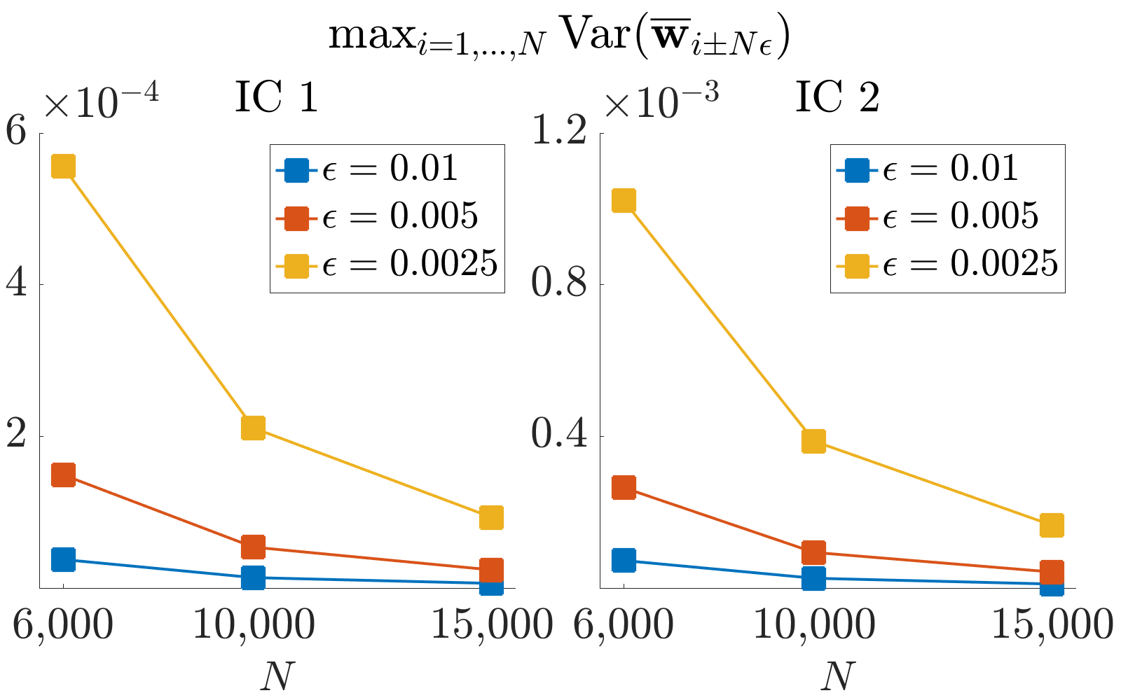
If the distribution of 𝐰Nsubscript𝐰𝑁\mathbf{w}_{N} is given exactly by a prototypical LE state (such as a slowly varying local Gibbs distribution), then the expectations 𝔼[wi]𝔼delimited-[]subscript𝑤𝑖\mathbb{E}\,[w_{i}] vary smoothly over lattice sites i𝑖i, and the marginals Law(wi)Lawsubscript𝑤𝑖{\mathrm{Law}}(w_{i}) belong to a family of measures which can be parameterized by their means. Thanks to these and a few other properties, (V), (E), and (Ef) are easily satisfied. In fact, (V) and stronger limits (E\,{}^{\prime}) and (Ef\,{}^{\prime}) hold for the prototypical LE. Although for finite N𝑁N, Law(𝐰N)Lawsubscript𝐰𝑁{\mathrm{Law}}(\mathbf{w}_{N}) is never exactly a prototypical LE state, we show numerically for a simple, zero range process that Law(𝐰N)Lawsubscript𝐰𝑁{\mathrm{Law}}(\mathbf{w}_{N}) does satisfy the stronger limits. We should note that investigation of standard LE states is a secondary focus; the numerical results are shown primarily for the purpose of contrasting the standard LE to that of our crystal surface process.

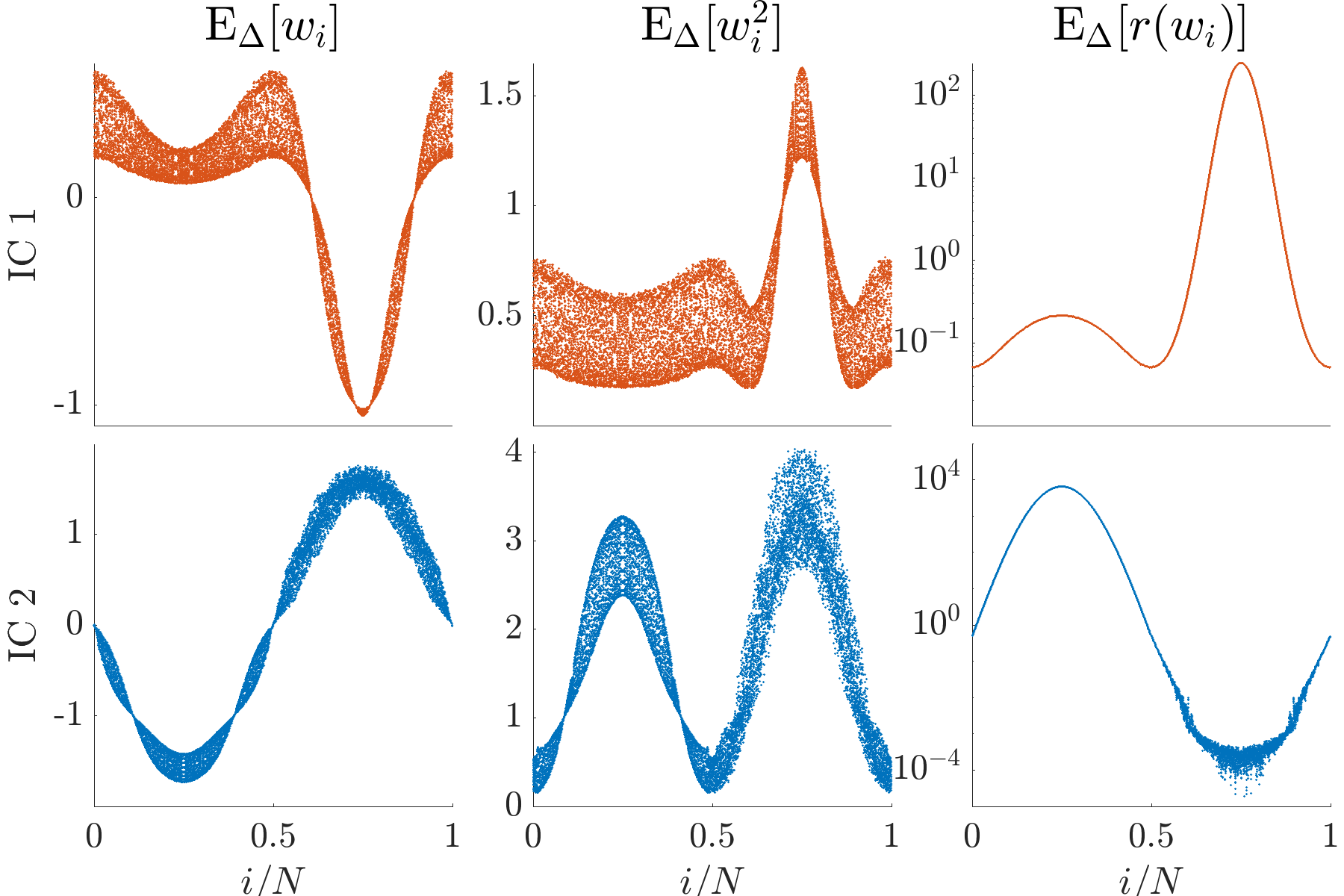
The essential difference is that in our case the Law(wi)Lawsubscript𝑤𝑖{\mathrm{Law}}(w_{i}) do not belong to a mean-parameterized measure family, and 𝔼wi𝔼subscript𝑤𝑖\mathbb{E}\,w_{i} do not vary smoothly with i𝑖i, nor do most observables 𝔼f(wi)𝔼𝑓subscript𝑤𝑖\mathbb{E}\,f(w_{i}). It would be unsurprising if the random wisubscript𝑤𝑖w_{i} varied roughly (a term we will define formally), but the rough variation of expectations is surprising and novel. The expectations 𝔼wi𝔼subscript𝑤𝑖\mathbb{E}\,w_{i} are rough even if the initial condition 𝐰N(0)subscript𝐰𝑁0\mathbf{w}_{N}(0) is chosen so that 𝔼wi(0)=w0(i/N)𝔼subscript𝑤𝑖0subscript𝑤0𝑖𝑁\mathbb{E}\,w_{i}(0)=w_{0}(i/N) for a smooth function w0(x)subscript𝑤0𝑥w_{0}(x).

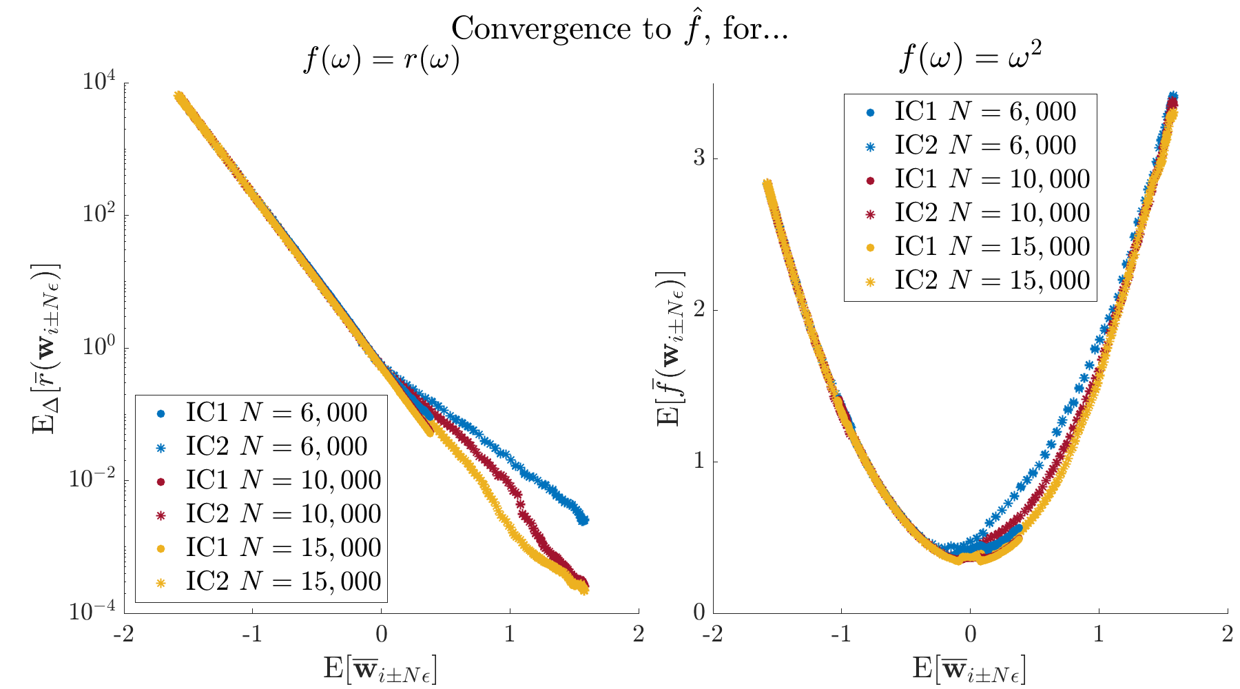
Our first main contribution is to show numerically that due to the rough behavior, the stronger limits are not satisfied, but despite the rough behavior, (V), (E), and (Ef) are still satisfied. We call this new kind of LE a “rough” LE state. Our second main contribution is theoretical. Using the numerically verified (E), and the additional numerically verified fact that Law(𝐰N)Lawsubscript𝐰𝑁{\mathrm{Law}}(\mathbf{w}_{N}) is induced by a local Gibbs measure, we rigorously prove that mesoscopic averages of the distributions Law(wi)Lawsubscript𝑤𝑖{\mathrm{Law}}(w_{i}) are measures which do belong to a certain mean-parameterized family, unlike the Law(wi)Lawsubscript𝑤𝑖{\mathrm{Law}}(w_{i}) themselves. This gives valuable insight about why (Ef) holds for a rough LE state.

We now give some background on the crystal surface process. Let 𝐡N(t)=(h1,N(t),,hN,N(t))subscript𝐡𝑁𝑡subscript1𝑁𝑡subscript𝑁𝑁𝑡{\bf h}_{N}(t)=(h_{1,N}(t),\dots,h_{N,N}(t)), where hi,Nsubscript𝑖𝑁h_{i,N} is the (discrete) height of a column, or number of particles, at site i𝑖i. The process evolves via jumps between neighboring lattice sites which tend to lower the surface energy on average. These jumps occur with so-called “Arrhenius” transition rates. For a review of the physics of crystal surfaces, including the Arrhenius rates, see [25]. The process 𝐰N(t)subscript𝐰𝑁𝑡\mathbf{w}_{N}(t) studied here tracks the “curvature” of this crystal surface height profile, or more precisely, the second order finite differences wi,N=hi+1,N2hi,N+hi1,Nsubscript𝑤𝑖𝑁subscript𝑖1𝑁2subscript𝑖𝑁subscript𝑖1𝑁w_{i,N}=h_{i+1,N}-2h_{i,N}+h_{i-1,N}. This curvature process is expected to have a nontrivial hydrodynamic limit provided 𝐡Nsubscript𝐡𝑁{\bf h}_{N} is scaled to have order O(N2)𝑂superscript𝑁2O(N^{2}) heights (see Definition 2.12.2 for precise statements). Marzuola and Weare introduced this scaling in [17], naming it the “rough” scaling regime for reasons independent of the rough LE discovered here. The authors use probabilistic but heuristic arguments to show that the hydrodynamic limit of N2𝐡Nsuperscript𝑁2subscript𝐡𝑁N^{-2}{\bf h}_{N} is a fourth order diffusion with exponential nonlinearity. Linearizing this exponential gives the PDE limit of the height process in the more standard, smooth scaling regime, first derived by Krug, Dobbs, and Majaniemi using physical arguments [14]. Recently, the rough scaling limit of an Arrhenius rate process with additional deposition and evaporation has also been derived [6], yielding a nonlinear fourth order PDE with a second order correction.

So far, none of these hydrodynamic limits have been proven rigorously, due in part to technical obstacles posed by the discrete heights. On the other hand, there are several continuous height variants of the crystal surface model for which rigorous hydrodynamic limits have been carried out. In [3], Funaki and Spohn prove the second order hydrodynamic limit of the Ginzburg-Landau ϕitalic-ϕ\nabla\phi interface model without conservation of mass. Using our notation, this means ihi,N(t)subscript𝑖subscript𝑖𝑁𝑡\sum_{i}h_{i,N}(t) can vary. In [18], Nishikawa proves the fourth order limit of the analogous dynamics with ihi,N(t)subscript𝑖subscript𝑖𝑁𝑡\sum_{i}h_{i,N}(t) conserved. In [19], Savu derives the hydrodynamic limit of a “nongradient” form of the continuous height model.

The dynamics of the 𝐰Nsubscript𝐰𝑁\mathbf{w}_{N} curvature process can be formulated independently of the 𝐡Nsubscript𝐡𝑁\mathbf{h}_{N} height process, so that studying the hydrodynamic limit of 𝐰Nsubscript𝐰𝑁\mathbf{w}_{N} independently of 𝐡Nsubscript𝐡𝑁\mathbf{h}_{N} is legitimate. In some sense in fact, the 𝐡Nsubscript𝐡𝑁\mathbf{h}_{N} limit is the one which depends on the 𝐰Nsubscript𝐰𝑁\mathbf{w}_{N} limit. As we argue in Section 6.4, the rough LE state of 𝐰Nsubscript𝐰𝑁\mathbf{w}_{N} explains an interesting difference noted in [17] between the rough and smooth PDE limits of the crystal surface height process: the differential operator of the smooth scaling PDE involves a function which “sees” the discreteness of the microscopic system, while the rough scaling differential operator involves an analogous function which does not. These and other insights significantly expand the current understanding of the convergence mechanism for the crystal surface process under rough scaling. In particular, we correct some of the claims in [17] used to derive the PDE limit of the height process.

Finally, we note that this new, “rough” LE is not limited to the curvature process of the Arrhenius rate crystal surface dynamics in the rough scaling regime. In the conclusion, we mention a second process with Metropolis-type jump rates, that has the same kind of LE structure. This is the subject of an upcoming paper [11].

1.1 Organization

In Section 2, we introduce the crystal surface model, define the notions of scaling regime and hydrodynamic limit, and review existing results on the crystal PDE limits. In Section 3, we explain our focus on three key limits. We then review the structure of standard LE states in Section 4, and give numerical evidence for the hypothesis that they satisfy the stronger limits (E\,{}^{\prime}) and (Ef\,{}^{\prime}). Section 5 contains our numerical case study of 𝐰Nsubscript𝐰𝑁\mathbf{w}_{N}’s rough LE state. In Section 6, we first state and numerically verify the explicit form of Law(wi)Lawsubscript𝑤𝑖{\mathrm{Law}}(w_{i}). We then use this form, in addition to the numerically confirmed (E), to rigorously prove that (Ef) holds thanks to mesoscopic averaging of Law(wi)Lawsubscript𝑤𝑖{\mathrm{Law}}(w_{i}). We make some concluding remarks in Section 7. The proofs and details of numerical simulations can be found in the appendix.

For maximal clarity, let us summarize the type of result (informal, numerical, or rigorous) presented in each section. Section 2 is a review which includes informal claims. The derivation of the PDE in Section 3 is also non-rigorous. It is intended only to motivate our study of (Ef) in addition to (V) and (E). All claims made in Sections 4 and 5 are confirmed numerically. All statements in Sections 6.2 and 6.3 are proven rigorously, using numerically verified assumptions stated explicitly in Section 6.1. Section 6.4 is again informal.

1.2 Notation

Given a sequence of vectors 𝐰NNsubscript𝐰𝑁superscript𝑁\mathbf{w}_{N}\in\mathbb{Z}^{N}, N=1,2,𝑁12N=1,2,\dots, we will suppress the dependence of the entries of 𝐰Nsubscript𝐰𝑁\mathbf{w}_{N} on N𝑁N, writing 𝐰N=(w1,,wN)subscript𝐰𝑁subscript𝑤1subscript𝑤𝑁\mathbf{w}_{N}=(w_{1},\dots,w_{N}). For a probability mass function (pmf) μ𝜇\mu over the integers, we write μ(f)𝜇𝑓\mu(f) to denote nf(n)μ(n)subscript𝑛𝑓𝑛𝜇𝑛\sum_{n}f(n)\mu(n), with the exception of f(n)=n𝑓𝑛𝑛f(n)=n. Instead we denote the first moment of μ𝜇\mu by m1(μ)subscript𝑚1𝜇m_{1}(\mu); that is, m1(μ)=nnμ(n)subscript𝑚1𝜇subscript𝑛𝑛𝜇𝑛m_{1}(\mu)=\sum_{n}n\mu(n). We will denote the parameter λ𝜆\lambda of a pmf in a parameterized family using square brackets: e.g. μ[λ]{μ[λ]λ}𝜇delimited-[]𝜆conditional-set𝜇delimited-[]𝜆𝜆\mu[\lambda]\in\{\mu[\lambda]\mid\lambda\in\mathbb{R}\}. The probability of n𝑛n under μ[λ]𝜇delimited-[]𝜆\mu[\lambda] is then μ[λ](n)𝜇delimited-[]𝜆𝑛\mu[\lambda](n). We let [0,1]01{[0,1]} denote the unit torus, and write iN(x±ϵ)𝑖𝑁plus-or-minus𝑥italic-ϵi\in{N(x\pm\epsilon)} to denote an integer i𝑖i such that |iNx|<Nϵ𝑖𝑁𝑥𝑁italic-ϵ|i-Nx|<N\epsilon. Also, C([0,1])𝐶01C({[0,1]}) is the space of continuous functions on the unit torus. Further notation will be introduced as needed.

Acknowledgments

I would like to thank Jonathan Weare for his guidance, patience, and insight throughout the research and writing process. I would also like to thank Jeremy Marzuola, who introduced me to the crystal surface problem and with whom I have had many useful discussions throughout the years. Finally, I am grateful for the computing resources that NYU High Performance Computing made available to me, and for the support of the DOE CSGF.

2 Microscopic Model and Hydrodynamic Limit

In 2.1, we introduce the crystal surface height, slope, and curvature process, describe the generators of these processes, and the invariant measure of the slope process. In 2.2, we define the notions of scaling regime and hydrodynamic limit, and review existing results on the PDE limits of the smooth and rough scaled crystal surface process.

2.1 Microscopic Model

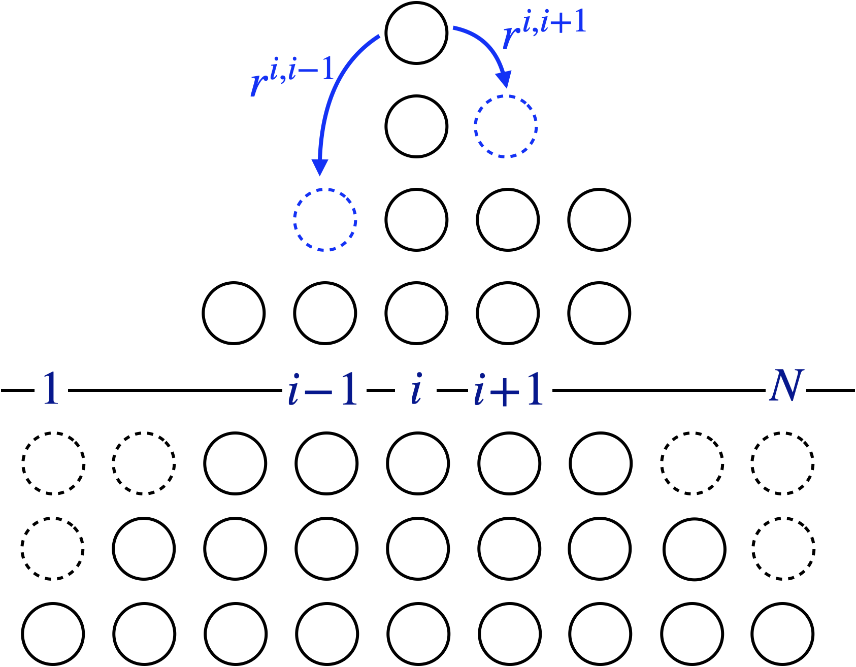
Consider a crystal surface as an arrangement of particles on a periodic lattice, as shown schematically in Figure 1. We represent the crystal surface height profile by a Markov jump process (𝐡~N(t))t0=(h~1(t),,h~N(t))t0subscriptsubscript~𝐡𝑁𝑡𝑡0subscriptsubscript~1𝑡subscript~𝑁𝑡𝑡0(\tilde{\mathbf{h}}_{N}(t))_{t\geq 0}=(\tilde{h}_{1}(t),\dots,\tilde{h}_{N}(t))_{t\geq 0} on Nsuperscript𝑁\mathbb{Z}^{N}. If h~i0subscript~𝑖0\tilde{h}_{i}\geq 0 then h~isubscript~𝑖\tilde{h}_{i} represents the number of particles stacked above level zero at lattice site i𝑖i, and if h~i<0subscript~𝑖0\tilde{h}_{i}<0 then |h~i|subscript~𝑖|\tilde{h}_{i}| represents the number of particles “missing” below level zero at lattice site i𝑖i, shown as black dotted circles in the figure. Since the lattice is periodic, we will use modmodulo\bmod N𝑁N indexing throughout.

The surface evolves through particle jumps between neighboring columns. Suppose a particle at the top of column i𝑖i jumps to a neighboring column j=i±1𝑗plus-or-minus𝑖1j=i\pm 1, as depicted in the figure (the red dotted circles denote the possible locations of the particle post-jump). If the particle configuration pre-jump is hh, then the particle configuration post-jump is hi,jsuperscript𝑖𝑗h^{i,j} defined as

(1) (hi,j)k={hi1,k=i,hj+1,k=j,hk,otherwise.subscriptsuperscript𝑖𝑗𝑘casessubscript𝑖1𝑘𝑖subscript𝑗1𝑘𝑗subscript𝑘otherwise.(h^{i,j})_{k}=\begin{cases}h_{i}-1,\quad&k=i,\\ h_{j}+1,\quad&k=j,\\ h_{k},\quad&\text{otherwise.}\end{cases}
Refer to caption
Figure 1: Schematic of crystal surface height process 𝐡~Nsubscript~𝐡𝑁\tilde{\mathbf{h}}_{N}.

These transitions hhi,jmaps-tosuperscript𝑖𝑗h\mapsto h^{i,j} are the only transitions which occur in the dynamics. The slope process is given by 𝐳~N(t)=(z~1(t),,z~N(t))subscript~𝐳𝑁𝑡subscript~𝑧1𝑡subscript~𝑧𝑁𝑡\tilde{\mathbf{z}}_{N}(t)=(\tilde{z}_{1}(t),\dots,\tilde{z}_{N}(t)), where z~i=h~i+1h~isubscript~𝑧𝑖subscript~𝑖1subscript~𝑖\tilde{z}_{i}=\tilde{h}_{i+1}-\tilde{h}_{i}. In this paper, we study the “curvature” process 𝐰~N(t)=(w~1(t),,w~N(t)),subscript~𝐰𝑁𝑡subscript~𝑤1𝑡subscript~𝑤𝑁𝑡\tilde{\mathbf{w}}_{N}(t)=(\tilde{w}_{1}(t),\dots,\tilde{w}_{N}(t)), where

w~i=z~iz~i1=h~i+12h~i+h~i1.subscript~𝑤𝑖subscript~𝑧𝑖subscript~𝑧𝑖1subscript~𝑖12subscript~𝑖subscript~𝑖1\tilde{w}_{i}=\tilde{z}_{i}-\tilde{z}_{i-1}=\tilde{h}_{i+1}-2\tilde{h}_{i}+\tilde{h}_{i-1}.

If 𝐡𝐡\mathbf{h} jumps to 𝐡i,jsuperscript𝐡𝑖𝑗\mathbf{h}^{i,j}, then we write that 𝐳𝐳\mathbf{z} jumps to 𝐳i,jsuperscript𝐳𝑖𝑗\mathbf{z}^{i,j}, and 𝐰𝐰\mathbf{w} jumps to 𝐰i,jsuperscript𝐰𝑖𝑗\mathbf{w}^{i,j}. Here, 𝐳i,jsuperscript𝐳𝑖𝑗\mathbf{z}^{i,j} (𝐰i,jsuperscript𝐰𝑖𝑗\mathbf{w}^{i,j}) denotes the slope profile (curvature profile) induced by 𝐡i,jsuperscript𝐡𝑖𝑗\mathbf{h}^{i,j}, where 𝐳𝐳\mathbf{z} is the slope of 𝐡𝐡\mathbf{h} (𝐰𝐰\mathbf{w} is the “curvature” of 𝐡𝐡\mathbf{h}). It is straightforward to see that 𝐳i,jsuperscript𝐳𝑖𝑗\mathbf{z}^{i,j} and 𝐰i,jsuperscript𝐰𝑖𝑗\mathbf{w}^{i,j} depend only on 𝐳𝐳\mathbf{z} and 𝐰𝐰\mathbf{w}, respectively. For example,

(2) (wi,i+1)k={wk1,k=i1,wk+3,k=i,wk3,k=i+1,wk+1,k=i+2,wk,otherwise,(wi+1,i)k={wk+1,k=i1,wk3,k=i,wk+3,k=i+1,wk1,k=i+2,wk,otherwise.formulae-sequencesubscriptsuperscript𝑤𝑖𝑖1𝑘casessubscript𝑤𝑘1𝑘𝑖1subscript𝑤𝑘3𝑘𝑖subscript𝑤𝑘3𝑘𝑖1subscript𝑤𝑘1𝑘𝑖2subscript𝑤𝑘otherwise,subscriptsuperscript𝑤𝑖1𝑖𝑘casessubscript𝑤𝑘1𝑘𝑖1subscript𝑤𝑘3𝑘𝑖subscript𝑤𝑘3𝑘𝑖1subscript𝑤𝑘1𝑘𝑖2subscript𝑤𝑘otherwise.(w^{i,i+1})_{k}=\begin{cases}w_{k}-1,\quad&k=i-1,\\ w_{k}+3,\quad&k=i,\\ w_{k}-3,\quad&k=i+1,\\ w_{k}+1,\quad&k=i+2,\\ w_{k},\quad&\text{otherwise,}\end{cases}\quad(w^{i+1,i})_{k}=\begin{cases}w_{k}+1,\quad&k=i-1,\\ w_{k}-3,\quad&k=i,\\ w_{k}+3,\quad&k=i+1,\\ w_{k}-1,\quad&k=i+2,\\ w_{k},\quad&\text{otherwise.}\end{cases}

Now, to each height profile we associate an energy, or Hamiltonian, that depends only on the corresponding slope profile,

H(𝐡)=H(𝐳)=i=1Nzi2.𝐻𝐡𝐻𝐳superscriptsubscript𝑖1𝑁superscriptsubscript𝑧𝑖2H(\mathbf{h})=H(\mathbf{z})=\sum_{i=1}^{N}z_{i}^{2}.

The quadratic potential is a modeling choice that makes the subsequent analysis easier. Another common choice is the absolute-value potential. Let us now define the Arrhenius transition rates. The rate of a jump from i𝑖i to i+1𝑖1i+1 is equal to the rate of a jump from i𝑖i to i1𝑖1i-1, and is given by

(3) ri(𝐡)=exp(K[H(Ji𝐡)H(𝐡)]),subscript𝑟𝑖𝐡exp𝐾delimited-[]𝐻subscript𝐽𝑖𝐡𝐻𝐡r_{i}(\mathbf{h})=\,\mathrm{exp}\left(-K\left[H(J_{i}\mathbf{h})-H(\mathbf{h})\right]\right),

where K𝐾K is a system parameter which can be thought of as inverse temperature, and Ji𝐡subscript𝐽𝑖𝐡J_{i}\mathbf{h} is obtained from 𝐡𝐡\mathbf{h} by decreasing the height at site i𝑖i by 1. The physical intuition underlying these rates is that in order for a particle at site i𝑖i to jump to a neighboring column j=i±1𝑗plus-or-minus𝑖1j=i\pm 1, it first breaks the bonds holding it in place, and then jumps left or right with equal probability. The amount of energy needed to break the bonds is the energy change induced by removing the particle, i.e. H(Ji𝐡)H(𝐡)𝐻subscript𝐽𝑖𝐡𝐻𝐡H(J_{i}\mathbf{h})-H(\mathbf{h}). Note that 𝐡Ji𝐡maps-to𝐡subscript𝐽𝑖𝐡\mathbf{h}\mapsto J_{i}\mathbf{h} is not itself an allowable transition under the dynamics. Define

(4) r(w)=e2K2Kw.𝑟𝑤superscript𝑒2𝐾2𝐾𝑤r(w)=e^{-2K-2Kw}.

Working out the transition rates explicitly by expanding the Hamiltonians, we get

ri(𝐡)=e2K2K(zizi1)=r(wi).subscript𝑟𝑖𝐡superscript𝑒2𝐾2𝐾subscript𝑧𝑖subscript𝑧𝑖1𝑟subscript𝑤𝑖r_{i}(\mathbf{h})=e^{-2K-2K(z_{i}-z_{i-1})}=r(w_{i}).

Since the jumps 𝐡𝐡i,i±1maps-to𝐡superscript𝐡𝑖plus-or-minus𝑖1\mathbf{h}\mapsto\mathbf{h}^{i,i\pm 1} occur with rates ri(𝐡)=r(wi)subscript𝑟𝑖𝐡𝑟subscript𝑤𝑖r_{i}(\mathbf{h})=r(w_{i}), depending only on the curvatures wisubscript𝑤𝑖w_{i}, it follows that 𝐳~N(t)subscript~𝐳𝑁𝑡\tilde{\mathbf{z}}_{N}(t) and 𝐰~N(t)subscript~𝐰𝑁𝑡\tilde{\mathbf{w}}_{N}(t) are both also Markov jump processes which can be defined independently of 𝐡~N(t)subscript~𝐡𝑁𝑡\tilde{\mathbf{h}}_{N}(t). For example the dynamics of 𝐰~N(t)subscript~𝐰𝑁𝑡\tilde{\mathbf{w}}_{N}(t) is given by the Markov jump process with jumps 𝐰𝐰i,i±1maps-to𝐰superscript𝐰𝑖plus-or-minus𝑖1\mathbf{w}\mapsto\mathbf{w}^{i,i\pm 1} occurring at rates r(wi)𝑟subscript𝑤𝑖r(w_{i}), i=1,,N𝑖1𝑁i=1,\dots,N. More formally, the dynamics of 𝐰~Nsubscript~𝐰𝑁\tilde{\mathbf{w}}_{N} is given by the generator

(5) (Nf)(𝐰)=i=1Nr(wi)([f(𝐰i,i+1)f(𝐰)]+[f(𝐰i,i1)f(𝐰)]).subscript𝑁𝑓𝐰superscriptsubscript𝑖1𝑁𝑟subscript𝑤𝑖delimited-[]𝑓superscript𝐰𝑖𝑖1𝑓𝐰delimited-[]𝑓superscript𝐰𝑖𝑖1𝑓𝐰\begin{split}(\mathcal{L}_{N}f)(\mathbf{w})&=\sum_{i=1}^{N}r(w_{i})\left(\left[f(\mathbf{w}^{i,i+1})-f(\mathbf{w})\right]+\left[f(\mathbf{w}^{i,i-1})-f(\mathbf{w})\right]\right).\end{split}

For example, let πj:(w1,,wN)wj:subscript𝜋𝑗maps-tosubscript𝑤1subscript𝑤𝑁subscript𝑤𝑗\pi_{j}:(w_{1},\dots,w_{N})\mapsto w_{j} denote the projection onto the j𝑗jth coordinate. Recalling the transition operators 𝐰𝐰i,jmaps-to𝐰superscript𝐰𝑖𝑗\mathbf{w}\mapsto\mathbf{w}^{i,j} in (2), we compute that

(6) (Nπj)(𝐰)=r(wj2)4r(wj1)+6r(wj)4r(wj+1)+r(wj+2).subscript𝑁subscript𝜋𝑗𝐰𝑟subscript𝑤𝑗24𝑟subscript𝑤𝑗16𝑟subscript𝑤𝑗4𝑟subscript𝑤𝑗1𝑟subscript𝑤𝑗2(\mathcal{L}_{N}\pi_{j})(\mathbf{w})=r(w_{j-2})-4r(w_{j-1})+6r(w_{j})-4r(w_{j+1})+r(w_{j+2}).

The generator determines the evolution of an initial measure. For example, if 𝐰~N(0)μ0Nsimilar-tosubscript~𝐰𝑁0subscriptsuperscript𝜇𝑁0\tilde{\mathbf{w}}_{N}(0)\sim\mu^{N}_{0} then

𝐰~N(t)μ0NetN,similar-tosubscript~𝐰𝑁𝑡subscriptsuperscript𝜇𝑁0superscript𝑒𝑡subscript𝑁\tilde{\mathbf{w}}_{N}(t)\sim\mu^{N}_{0}e^{t\mathcal{L}_{N}},

where multiplication on the right denotes application of the adjoint operator. The process 𝐳~Nsubscript~𝐳𝑁\tilde{\mathbf{z}}_{N} has the special property — not shared by 𝐡~Nsubscript~𝐡𝑁\tilde{\mathbf{h}}_{N} and 𝐰~Nsubscript~𝐰𝑁\tilde{\mathbf{w}}_{N} — that it is invariant with respect to a product measure, specifically the Gibbs measure

(7) ΦN(𝐳)=i=1Nexp(Kzi2)𝒵=eKH(𝐳)𝒵N,𝒵=nexp(Kn2).formulae-sequencesubscriptΦ𝑁𝐳superscriptsubscriptproduct𝑖1𝑁exp𝐾superscriptsubscript𝑧𝑖2𝒵superscript𝑒𝐾𝐻𝐳superscript𝒵𝑁𝒵subscript𝑛exp𝐾superscript𝑛2\Phi_{N}(\mathbf{z})=\prod_{i=1}^{N}\frac{\,\mathrm{exp}\left(-Kz_{i}^{2}\right)}{\mathcal{Z}}=\frac{e^{-KH(\mathbf{z})}}{\mathcal{Z}^{N}},\quad\mathcal{Z}=\sum_{n\in\mathbb{Z}}\,\mathrm{exp}\left(-Kn^{2}\right).

The invariance of ΦNsubscriptΦ𝑁\Phi_{N} under the 𝐳~Nsubscript~𝐳𝑁\tilde{\mathbf{z}}_{N} dynamics is a consequence of detailed balance:

ri(𝐳)ΦN(𝐳)=ri+1(𝐳i,i+1)ΦN(𝐳i,i+1)i=1,,N,𝐳N.formulae-sequencesubscript𝑟𝑖𝐳subscriptΦ𝑁𝐳subscript𝑟𝑖1superscript𝐳𝑖𝑖1subscriptΦ𝑁superscript𝐳𝑖𝑖1formulae-sequencefor-all𝑖1𝑁for-all𝐳superscript𝑁r_{i}(\mathbf{z})\Phi_{N}(\mathbf{z})=r_{i+1}(\mathbf{z}^{i,i+1})\Phi_{N}(\mathbf{z}^{i,i+1})\quad\forall i=1,\dots,N,\,\forall\mathbf{z}\in\mathbb{Z}^{N}.

That the Arrhenius rates satisfy detailed balance is straightforward to see from their original formulation (3) in terms of Hamiltonians. Also, one can show that the transitions 𝐳𝐳i,jmaps-to𝐳superscript𝐳𝑖𝑗\mathbf{z}\mapsto\mathbf{z}^{i,j} do not change the values of S0(𝐳)=kzksubscript𝑆0𝐳subscript𝑘subscript𝑧𝑘S_{0}(\mathbf{z})=\sum_{k}z_{k} and S1(𝐳)=kkzksubscript𝑆1𝐳subscript𝑘𝑘subscript𝑧𝑘S_{1}(\mathbf{z})=\sum_{k}kz_{k}, so the ergodic measures are the restrictions of ΦNsubscriptΦ𝑁\Phi_{N} to (S0,S1)subscript𝑆0subscript𝑆1(S_{0},S_{1}) level sets.

2.2 Hydrodynamic Limit

Let us take a step back to discuss the connected notions of scaling regime and hydrodynamic limit for a sequence of microscopic processes 𝐯~Nsubscript~𝐯𝑁\tilde{\mathbf{v}}_{N} defined on Nsuperscript𝑁\mathbb{Z}^{N}. The letter v𝑣v will always denote a generic process.

The idea of a hydrodynamic limit is that, if we zoom out from a microscopic process, a macroscopic dynamics will emerge. How to zoom out depends on several characteristic scales of the microscopic process. For stochastic lattice gases such as the crystal surface model, one of these scales is spatial: the lattice width N𝑁N. A second scale to consider is temporal: as N𝑁N increases, it takes longer for local changes to have a global effect on the stochastic lattice gas. We therefore associate to macroscopic times ΔtΔ𝑡\Delta t the microscopic time NαΔtsuperscript𝑁𝛼Δ𝑡N^{\alpha}\Delta t, for some α>0𝛼0\alpha>0. A third characteristic scale, relevant to unbounded microscopic processes such as the crystal surface, is the amplitude of the process itself. For example, consider the slope process 𝐳~Nsubscript~𝐳𝑁\tilde{\mathbf{z}}_{N} associated to a crystal surface height process. The “smoothness” of the crystal can be measured by the magnitude Nβsuperscript𝑁𝛽N^{\beta} of these slopes. Rougher crystals have larger β𝛽\beta. The transition rates will apply a greater force (so to speak) to smoothen rougher surfaces.

To obtain a hydrodynamic limit, we must first rescale the process 𝐯Nsubscript𝐯𝑁\mathbf{v}_{N}. Let

𝐯N(t)=𝐯~N(Nαt).subscript𝐯𝑁𝑡subscript~𝐯𝑁superscript𝑁𝛼𝑡\mathbf{v}_{N}(t)=\tilde{\mathbf{v}}_{N}(N^{\alpha}t).

The spatial rescaling occurs by interpreting 𝐯N(t)subscript𝐯𝑁𝑡\mathbf{v}_{N}(t) as a random step function on the unit interval, or more formally, a random measure:

(8) vN(t,dx)=1Ni=1Nvi(t)δ(xiN).subscript𝑣𝑁𝑡𝑑𝑥1𝑁superscriptsubscript𝑖1𝑁subscript𝑣𝑖𝑡𝛿𝑥𝑖𝑁v_{N}(t,dx)=\frac{1}{N}\sum_{i=1}^{N}v_{i}(t)\delta\left(x-\frac{i}{N}\right).

Finally, we encode the amplitude scaling into the 𝐯Nsubscript𝐯𝑁\mathbf{v}_{N} initial condition, and into the definition of hydrodynamic limit.

Definition 2.1.

We say the sequence of measures μ0Nsubscriptsuperscript𝜇𝑁0\mu^{N}_{0} on Nsuperscript𝑁\mathbb{Z}^{N} is associated with a profile v0(x)subscript𝑣0𝑥v_{0}(x) under amplitude scaling Nβsuperscript𝑁𝛽N^{\beta} if

(9) μ0N((v1,,vN):|1Ni=1Nϕ(iN)[Nβvi][0,1]ϕ(x)v0(x)dx|>δ)0\mu^{N}_{0}\left((v_{1},\dots,v_{N})\;:\;\left|\frac{1}{N}\sum_{i=1}^{N}\phi\left(\frac{i}{N}\right)\left[N^{-\beta}v_{i}\right]-\int_{[0,1]}\phi(x)v_{0}(x)dx\right|>\delta\right)\to 0

as N𝑁N\to\infty for all ϕC([0,1])italic-ϕ𝐶01\phi\in C({[0,1]}) and δ>0𝛿0\delta>0.

As an example, the product measure μ0Nsubscriptsuperscript𝜇𝑁0\mu^{N}_{0} with marginals

viNβv0(i/N)+Bernoulli(1{Nβv0(i/N)})similar-tosubscript𝑣𝑖superscript𝑁𝛽subscript𝑣0𝑖𝑁Bernoulli1superscript𝑁𝛽subscript𝑣0𝑖𝑁v_{i}\;\sim\;\lfloor N^{\beta}v_{0}(i/N)\rfloor+\mathrm{Bernoulli}(1-\{N^{\beta}v_{0}(i/N)\})

satisfies (9). Here, {q}=qq𝑞𝑞𝑞\{q\}=q-\lfloor q\rfloor denotes the fractional part of q𝑞q.

Definition 2.2 (Hydrodynamic Limit).

Let 𝐯~Nsubscript~𝐯𝑁\tilde{\mathbf{v}}_{N} be a sequence of random processes on Nsuperscript𝑁\mathbb{Z}^{N}. We say the sequence 𝐯N(t)=𝐯~N(Nαt)subscript𝐯𝑁𝑡subscript~𝐯𝑁superscript𝑁𝛼𝑡\mathbf{v}_{N}(t)=\tilde{\mathbf{v}}_{N}(N^{\alpha}t) has a hydrodynamic limit v:[0,T]×[0,1]:𝑣0𝑇01v:[0,T]\times{[0,1]}\to\mathbb{R} under amplitude scaling Nβsuperscript𝑁𝛽N^{\beta} if for each t[0,T]𝑡0𝑇t\in[0,T], ϕC([0,1])italic-ϕ𝐶01\phi\in C({[0,1]}), and δ>0𝛿0\delta>0 we have

(10) (|1Ni=1Nϕ(iN)[Nβvi(t)][0,1]ϕ(u)v(t,u)𝑑u|>δ)0,N.formulae-sequence1𝑁superscriptsubscript𝑖1𝑁italic-ϕ𝑖𝑁delimited-[]superscript𝑁𝛽subscript𝑣𝑖𝑡subscript01italic-ϕ𝑢𝑣𝑡𝑢differential-d𝑢𝛿0𝑁\mathbb{P}\left(\left|\frac{1}{N}\sum_{i=1}^{N}\phi\left(\frac{i}{N}\right)\left[N^{-\beta}v_{i}(t)\right]-\int_{[0,1]}\phi(u)v(t,u)du\right|>\delta\right)\to 0,\quad N\to\infty.

In (10), the probability distribution on 𝐯N(t)subscript𝐯𝑁𝑡\mathbf{v}_{N}(t) is given by

(𝐯N(t)A)=(𝐯~N(Nαt)A)=μtN(A),subscript𝐯𝑁𝑡𝐴subscript~𝐯𝑁superscript𝑁𝛼𝑡𝐴subscriptsuperscript𝜇𝑁𝑡𝐴\mathbb{P}(\mathbf{v}_{N}(t)\in A)=\mathbb{P}(\tilde{\mathbf{v}}_{N}(N^{\alpha}t)\in A)=\mu^{N}_{t}(A),

where μtN:=μ0Nexp(NαtN).assignsubscriptsuperscript𝜇𝑁𝑡subscriptsuperscript𝜇𝑁0expsuperscript𝑁𝛼𝑡subscript𝑁\mu^{N}_{t}:=\mu^{N}_{0}\,\mathrm{exp}(N^{\alpha}t\mathcal{L}_{N}). Given α,β𝛼𝛽\alpha,\beta, and a sequence of processes 𝐯~N(t)subscript~𝐯𝑁𝑡\tilde{\mathbf{v}}_{N}(t) with generators Nsubscript𝑁\mathcal{L}_{N}, the main goals are (1) to prove that 𝐯N(t)=𝐯~N(Nαt)subscript𝐯𝑁𝑡subscript~𝐯𝑁superscript𝑁𝛼𝑡\mathbf{v}_{N}(t)=\tilde{\mathbf{v}}_{N}(N^{\alpha}t) has a hydrodynamic limit v𝑣v under amplitude scaling Nβsuperscript𝑁𝛽N^{\beta}, and (2) to determine the PDE governing the evolution of v𝑣v. Typically, these goals are intertwined and achieved together in rigorous proofs. Of course, we only expect there to be a nontrivial PDE limit if 𝐯~Nsubscript~𝐯𝑁\tilde{\mathbf{v}}_{N} is initialized appropriately, i.e. if 𝐯~N(0)μ0Nsimilar-tosubscript~𝐯𝑁0subscriptsuperscript𝜇𝑁0\tilde{\mathbf{v}}_{N}(0)\sim\mu^{N}_{0} is associated to a smooth v0subscript𝑣0v_{0} under amplitude scaling Nβsuperscript𝑁𝛽N^{\beta}. The function v0subscript𝑣0v_{0} is then the initial condition of the PDE.

Let us now return to the crystal surface models. In [14] and [17], the authors study the Arrhenius rate discrete height process 𝐡~Nsubscript~𝐡𝑁\tilde{\mathbf{h}}_{N} in the smooth scaling regime (the name was coined in the latter paper). In this regime, one takes the hydrodynamic limit of 𝐡N(t)=𝐡~N(N4t)subscript𝐡𝑁𝑡subscript~𝐡𝑁superscript𝑁4𝑡\mathbf{h}_{N}(t)=\tilde{\mathbf{h}}_{N}(N^{4}t) under amplitude scaling N1superscript𝑁1N^{1}. Note that the amplitude scaling has a nonlinear effect on the dynamics, i.e. (Nπi)(Nh)N(Nπi)(h)subscript𝑁subscript𝜋𝑖𝑁𝑁subscript𝑁subscript𝜋𝑖(\mathcal{L}_{N}\pi_{i})(Nh)\neq N(\mathcal{L}_{N}\pi_{i})(h) since the rates are exponential in wi=hi+12hi+hi1subscript𝑤𝑖subscript𝑖12subscript𝑖subscript𝑖1w_{i}=h_{i+1}-2h_{i}+h_{i-1}. These papers show using nonrigorous arguments that in the smooth scaling regime, the hydrodynamic limit hh solves

(11) th=xxxλD(xh).subscript𝑡subscript𝑥𝑥𝑥subscript𝜆𝐷subscript𝑥\partial_{t}h=-\partial_{xxx}\lambda_{D}(\partial_{x}h).

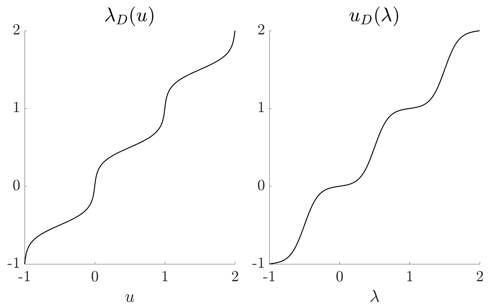
Here, λD(u)=u+λo(u)subscript𝜆𝐷𝑢𝑢subscript𝜆𝑜𝑢\lambda_{D}(u)=u+\lambda_{o}(u), where λosubscript𝜆𝑜\lambda_{o} is a smooth periodic perturbation with period one (the function λDsubscript𝜆𝐷\lambda_{D} is denoted σDsubscript𝜎𝐷\sigma_{D} in [17]). We will discuss this function and the smooth scaling PDE in Section 6. Marzuola and Weare also propose a non-standard, “rough” scaling regime in [17], which is our interest here. In the rough scaling regime, one takes the hydrodynamic limit of 𝐡N(t)=𝐡~N(N4t)subscript𝐡𝑁𝑡subscript~𝐡𝑁superscript𝑁4𝑡\mathbf{h}_{N}(t)=\tilde{\mathbf{h}}_{N}(N^{4}t) under amplitude scaling N2superscript𝑁2N^{2}. Through a heuristic argument supported by numerical simulations [17], the authors conclude that the rough scaling limit hh of 𝐡Nsubscript𝐡𝑁\mathbf{h}_{N} solves

(12) {ht=xxe2Khxx,t>0,h(0,x)=h0(x),x[0,1].casessubscript𝑡subscript𝑥𝑥superscript𝑒2𝐾subscript𝑥𝑥𝑡00𝑥subscript0𝑥𝑥01\begin{cases}h_{t}=\partial_{xx}\,e^{-2Kh_{xx}},\quad&t>0,\\ h(0,x)=h_{0}(x),\quad&x\in{[0,1]}.\end{cases}

Existence, uniqueness, and regularity of solutions to this PDE and variations of it have been studied e.g. in [16, 7, 15, 9, 1]. Liu and Xu [16], and Gao, Liu, and Lu [7] show that singularities can form in hxx(t,)subscript𝑥𝑥𝑡h_{xx}(t,\cdot) even when h0subscript0h_{0} is smooth. However, Ambrose proves that if h0subscript0h_{0} is analytic, and if h0′′𝔸subscriptnormsuperscriptsubscript0′′𝔸\|h_{0}^{\prime\prime}\|_{\mathbb{A}} is sufficiently small, then there exists a strong, analytic solution h(t,x)𝑡𝑥h(t,x) to (12) with growing radius of analyticity [1]. Here, u𝔸=k|u^(k)|subscriptnorm𝑢𝔸subscript𝑘^𝑢𝑘\|u\|_{\mathbb{A}}=\sum_{k\in\mathbb{Z}}|\hat{u}(k)|, where u^(k)^𝑢𝑘\hat{u}(k) is the k𝑘kth Fourier coefficient of u^^𝑢\hat{u}.

In this paper, we study the hydrodynamic limit of 𝐰N(t)=𝐰~N(N4t)subscript𝐰𝑁𝑡subscript~𝐰𝑁superscript𝑁4𝑡\mathbf{w}_{N}(t)=\tilde{\mathbf{w}}_{N}(N^{4}t) under amplitude scaling N0superscript𝑁0N^{0}. As discussed, this process can be defined independently of 𝐡~N(t)subscript~𝐡𝑁𝑡\tilde{\mathbf{h}}_{N}(t). This scaling corresponds to the rough scaling regime for 𝐡~Nsubscript~𝐡𝑁\tilde{\mathbf{h}}_{N}.

Remark 2.3.

Note that if 𝐡N(t)=𝐡~N(N4t)subscript𝐡𝑁𝑡subscript~𝐡𝑁superscript𝑁4𝑡\mathbf{h}_{N}(t)=\tilde{\mathbf{h}}_{N}(N^{4}t) has a hydrodynamic limit under amplitude scaling N2superscript𝑁2N^{2}, this does not imply that 𝐰N(t)subscript𝐰𝑁𝑡\mathbf{w}_{N}(t) has a hydrodynamic limit under amplitude scaling N0=1superscript𝑁01N^{0}=1. Meanwhile, the converse is likely true under some technical assumptions. This is due to the fact that if ϕC([0,1])italic-ϕ𝐶01\phi\in C({[0,1]}) then ϕ′′superscriptitalic-ϕ′′\phi^{\prime\prime} need not belong to C([0,1])𝐶01C({[0,1]}) (or even exist), while there is always a periodic ΦC([0,1])Φ𝐶01\Phi\in C({[0,1]}) such that Φ′′=ϕsuperscriptΦ′′italic-ϕ\Phi^{\prime\prime}=\phi. In general, we expect the hydrodynamic limit of an antiderivative to follow from the hydrodynamic limit of the derivative, not vice versa.

The above remark shows we cannot rigorously deduce the limit of 𝐰Nsubscript𝐰𝑁\mathbf{w}_{N} from the limit of 𝐡Nsubscript𝐡𝑁\mathbf{h}_{N}. Nevertheless, based on our knowledge of the hydrodynamic limit of 𝐡Nsubscript𝐡𝑁\mathbf{h}_{N}, we anticipate that the hydrodynamic limit of 𝐰N(t)=𝐰~N(N4t)subscript𝐰𝑁𝑡subscript~𝐰𝑁superscript𝑁4𝑡\mathbf{w}_{N}(t)=\tilde{\mathbf{w}}_{N}(N^{4}t) is the weak solution to

(13) {wt=xxxxe2Kw,t>0,w(0,x)=w0(x),x[0,1]casessubscript𝑤𝑡subscript𝑥𝑥𝑥𝑥superscript𝑒2𝐾𝑤𝑡0𝑤0𝑥subscript𝑤0𝑥𝑥01\begin{cases}w_{t}=\partial_{xxxx}\,e^{-2Kw},\quad&t>0,\\ w(0,x)=w_{0}(x),\quad&x\in{[0,1]}\end{cases}

with periodic boundary. For future reference, we define

(14) r^(w)=e2Kw,^𝑟𝑤superscript𝑒2𝐾𝑤\hat{r}(w)=e^{-2Kw},

the nonlinear function in the PDE (13).

In our numerical simulations, we will always take w0=h0′′subscript𝑤0superscriptsubscript0′′w_{0}=h_{0}^{\prime\prime} for some analytic h0subscript0h_{0} with w0𝔸subscriptnormsubscript𝑤0𝔸\|w_{0}\|_{\mathbb{A}} small, so that we can use the analyticity result of [1] to conclude that there is an analytic, strong solution h(t,x)𝑡𝑥h(t,x) to (12) and hence xxh(t,x)subscript𝑥𝑥𝑡𝑥\partial_{xx}h(t,x) is an analytic strong solution to (13). Although other non-analytic weak solutions to (13) could exist, we find numerically that 𝐰N(t)subscript𝐰𝑁𝑡\mathbf{w}_{N}(t) always converges to a smooth function w(t,)𝑤𝑡w(t,\cdot).

The reason to study 𝐰Nsubscript𝐰𝑁\mathbf{w}_{N} — specifically, the probability distribution of 𝐰N(t)subscript𝐰𝑁𝑡\mathbf{w}_{N}(t) once “local equilibrium” has been reached — is that doing so will uncover very interesting new phenomena overlooked in a study of 𝐡Nsubscript𝐡𝑁\mathbf{h}_{N} alone. The most striking phenomenon is the roughness of the (𝔼wi)i=1Nsuperscriptsubscript𝔼subscript𝑤𝑖𝑖1𝑁(\mathbb{E}\,w_{i})_{i=1}^{N} profile mentioned in the introduction. Note that this roughness in the microscopic system is not related to any potential singularity formation in solutions to the PDE (13), since we take initial data to ensure the PDE has a strong analytic solution.

3 Three Key Limits within Hydrodynamic Convergence

In this section, we introduce the three key limits we focus on in this paper, which expose important properties of the process. The first two limits express that 𝐰Nsubscript𝐰𝑁\mathbf{w}_{N} converges to a macroscopic w𝑤w. The third limit helps determine the PDE governing w𝑤w. To motivate this third limit, we will sketch the PDE derivation assuming the first two limits hold. It is important to emphasize that this PDE derivation is informal, and primarily serves as inspiration to study the third limit in addition to the first two.

Before proceeding, we introduce some notation. For ϕL([0,1])italic-ϕsuperscript𝐿01\phi\in L^{\infty}({[0,1]}) and wN(t,dx)subscript𝑤𝑁𝑡𝑑𝑥w_{N}(t,dx) given by the random measure intepretation of 𝐰N(t)subscript𝐰𝑁𝑡\mathbf{w}_{N}(t) (recall (8)), we define

(15) (ϕwN(t))(x)=[0,1]ϕ(xy)wN(t,dy).italic-ϕsubscript𝑤𝑁𝑡𝑥subscript01italic-ϕ𝑥𝑦subscript𝑤𝑁𝑡𝑑𝑦(\phi\ast w_{N}(t))(x)=\int_{[0,1]}\phi(x-y)w_{N}(t,dy).

Also, for a vector 𝐯=(v1,,vN)𝐯subscript𝑣1subscript𝑣𝑁\mathbf{v}=(v_{1},\dots,v_{N}) and a function f::𝑓f:\mathbb{R}\to\mathbb{R}, define

𝐯¯N(x±ϵ)=12NϵiN(x±ϵ)vi,f¯(𝐯N(x±ϵ))=12NϵiN(x±ϵ)f(vi).formulae-sequencesubscript¯𝐯𝑁plus-or-minus𝑥italic-ϵ12𝑁italic-ϵsubscript𝑖𝑁plus-or-minus𝑥italic-ϵsubscript𝑣𝑖¯𝑓subscript𝐯𝑁plus-or-minus𝑥italic-ϵ12𝑁italic-ϵsubscript𝑖𝑁plus-or-minus𝑥italic-ϵ𝑓subscript𝑣𝑖\begin{split}\overline{\bf v}_{{N(x\pm\epsilon)}}&=\frac{1}{2N\epsilon}\sum_{{i\in{N(x\pm\epsilon)}}}v_{i},\\ \bar{f}({\bf v}_{{N(x\pm\epsilon)}})&=\frac{1}{2N\epsilon}\sum_{{i\in{N(x\pm\epsilon)}}}f(v_{i}).\end{split}

Now, instead of the usual convergence (10) given in the hydrodynamic limit definition, we will consider a slightly more physically intuitive convergence. Namely, we will study whether the following holds:

(16) limϵ0limN𝔼|12NϵiN(x±ϵ)wi(t)w(t,x)|2=0,t>0,x[0,1].formulae-sequencesubscriptitalic-ϵ0subscript𝑁𝔼superscript12𝑁italic-ϵsubscript𝑖𝑁plus-or-minus𝑥italic-ϵsubscript𝑤𝑖𝑡𝑤𝑡𝑥20formulae-sequencefor-all𝑡0𝑥01\lim_{\epsilon\to 0}\lim_{N\to\infty}\mathbb{E}\,\bigg{|}\frac{1}{2N\epsilon}\sum_{i\in{N(x\pm\epsilon)}}w_{i}(t)-w(t,x)\bigg{|}^{2}=0,\quad\forall t>0,x\in{[0,1]}.

(16) is somewhat stronger than (10), but not significantly. Suppose (10) holds, and consider taking ϕitalic-ϕ\phi to be ϕ(u)=ϕ^ϵ(xu)italic-ϕ𝑢subscript^italic-ϕitalic-ϵ𝑥𝑢\phi(u)=\hat{\phi}_{\epsilon}(x-u), where ϕ^ϵsubscript^italic-ϕitalic-ϵ\hat{\phi}_{\epsilon} is an even bump function centered at 00 with support in (ϵ,ϵ)italic-ϵitalic-ϵ(-\epsilon,\epsilon). By (10), we have that (𝐰N(t)ϕ^ϵ)(x)subscript𝐰𝑁𝑡subscript^italic-ϕitalic-ϵ𝑥(\mathbf{w}_{N}(t)\ast\hat{\phi}_{\epsilon})(x) converges as N𝑁N\to\infty to (w(t)ϕ^ϵ)(x)𝑤𝑡subscript^italic-ϕitalic-ϵ𝑥(w(t)\ast\hat{\phi}_{\epsilon})(x) in probability for each x[0,1]𝑥01x\in{[0,1]}. If w𝑤w is continuous in x𝑥x, then it is not hard to see that (𝐰N(t)ϕ^ϵ)(x)subscript𝐰𝑁𝑡subscript^italic-ϕitalic-ϵ𝑥(\mathbf{w}_{N}(t)\ast\hat{\phi}_{\epsilon})(x) converges as N𝑁N\to\infty and then ϵ0italic-ϵ0\epsilon\to 0 to w(t,x)𝑤𝑡𝑥w(t,x) (this means the probability that the two differ by more than δ𝛿\delta goes to zero in the double limit). In (16), we ask for a slightly stronger convergence than this, replacing the smooth function ϕ^ϵ(u)subscript^italic-ϕitalic-ϵ𝑢\hat{\phi}_{\epsilon}(u) by the indicator ϕϵ(u)=12ϵ𝟙(ϵ,ϵ)(u)subscriptitalic-ϕitalic-ϵ𝑢12italic-ϵsubscript1italic-ϵitalic-ϵ𝑢\phi_{\epsilon}(u)=\frac{1}{2\epsilon}\mathbbm{1}_{(-\epsilon,\epsilon)}(u) and convergence in probability by convergence in L2superscript𝐿2L^{2}.

The advantage of studying the convergence (16) is two-fold. First, it allows us to focus on properties of the process in local, mesoscopic regions of the lattice. “Mesoscopic” regions are intervals (xϵ,x+ϵ)𝑥italic-ϵ𝑥italic-ϵ(x-\epsilon,x+\epsilon) which have macroscopic length 2ϵ1much-less-than2italic-ϵ12\epsilon\ll 1, but which, for any fixed ϵitalic-ϵ\epsilon, contain a growing number of lattice sites 2Nϵ2𝑁italic-ϵ2N\epsilon, N𝑁N\to\infty. Second, convergence in L2superscript𝐿2L^{2} can be conveniently separated into convergence of expectations and vanishing variance. Namely, the convergence (16) is equivalent to

(17a) limϵ0limNVar(𝐰¯N(x±ϵ)(t))=0,subscriptitalic-ϵ0subscript𝑁Varsubscript¯𝐰𝑁plus-or-minus𝑥italic-ϵ𝑡0\displaystyle\lim_{\epsilon\to 0}\lim_{N\to\infty}\mathrm{Var}\left(\overline{\bf w}_{{N(x\pm\epsilon)}}(t)\right)=0,
(17b) limϵ0limN𝔼𝐰¯N(x±ϵ)(t)=w(t,x).subscriptitalic-ϵ0subscript𝑁𝔼subscript¯𝐰𝑁plus-or-minus𝑥italic-ϵ𝑡𝑤𝑡𝑥\displaystyle\lim_{\epsilon\to 0}\lim_{N\to\infty}\mathbb{E}\,\overline{\bf w}_{{N(x\pm\epsilon)}}(t)=w(t,x).

These are our first two limits of interest. The equation  (17a) is satisfied if e.g. the variances Var(wi\mathrm{Var}(w_{i}) remain bounded while the correlations Corr(wi,wj)Corrsubscript𝑤𝑖subscript𝑤𝑗\mathrm{Corr}(w_{i},w_{j}) decrease with N𝑁N, so that by averaging increasingly many wisubscript𝑤𝑖w_{i} (2Nϵ2𝑁italic-ϵ2N\epsilon of them, with N𝑁N\to\infty), the variance of the average goes to zero. The equation (17b) expresses that the mesoscopic spatial average of expectations 𝔼[wi]𝔼delimited-[]subscript𝑤𝑖\mathbb{E}\,[w_{i}] converges to the limiting profile w(t,x)𝑤𝑡𝑥w(t,x).

Now, assume there exists a limit w(t,x)𝑤𝑡𝑥w(t,x) such that (17b) holds. We will show that (17b), combined with one more limit, is “nearly” sufficient to deduce that w𝑤w is a weak solution to (13). We define “weak solution” to mean that for all smooth compactly supported functions ψ𝜓\psi and for all t>0𝑡0t>0 we have

(18) [0,1]ψ(x)[w(t,x)dxw0(x)]𝑑x=0t[0,1]ψ(4)(x)r^(w(s,x))𝑑s𝑑x.subscript01𝜓𝑥delimited-[]𝑤𝑡𝑥𝑑𝑥subscript𝑤0𝑥differential-d𝑥superscriptsubscript0𝑡subscript01superscript𝜓4𝑥^𝑟𝑤𝑠𝑥differential-d𝑠differential-d𝑥\int_{[0,1]}\psi(x)[w(t,x)dx-w_{0}(x)]dx=\int_{0}^{t}\int_{[0,1]}\psi^{(4)}(x)\hat{r}(w(s,x))dsdx.

The term “nearly” is a catch-all for the non-rigorous statements made below (again, the following derivation is only for the purpose of motivating the third limit). Using (17b) and the fact that 𝐰¯N(x±ϵ)(t)=(ϕϵwN(t))(x)subscript¯𝐰𝑁plus-or-minus𝑥italic-ϵ𝑡subscriptitalic-ϕitalic-ϵsubscript𝑤𝑁𝑡𝑥\overline{\bf w}_{{N(x\pm\epsilon)}}(t)=(\phi_{\epsilon}\ast w_{N}(t))(x), we have

(19) [0,1]ψ(x)w(t,x)𝑑x=limϵ0limN[0,1]ψ(x)𝔼[(ϕϵwN(t))(x)]𝑑x=limϵ0limN[0,1](ψϕϵ)(x)𝔼[wN(t,dx)],subscript01𝜓𝑥𝑤𝑡𝑥differential-d𝑥subscriptitalic-ϵ0subscript𝑁subscript01𝜓𝑥𝔼delimited-[]subscriptitalic-ϕitalic-ϵsubscript𝑤𝑁𝑡𝑥differential-d𝑥subscriptitalic-ϵ0subscript𝑁subscript01𝜓subscriptitalic-ϕitalic-ϵ𝑥𝔼delimited-[]subscript𝑤𝑁𝑡𝑑𝑥\begin{split}\int_{[0,1]}\psi(x)w(t,x)dx&=\lim_{\epsilon\to 0}\lim_{N\to\infty}\int_{[0,1]}\psi(x)\mathbb{E}\,\left[(\phi_{\epsilon}\ast w_{N}(t))(x)\right]dx\\ &=\lim_{\epsilon\to 0}\lim_{N\to\infty}\int_{[0,1]}(\psi\ast\phi_{\epsilon})(x)\mathbb{E}\,[w_{N}(t,dx)],\end{split}

so that

(20) [0,1]ψ(x)[w(t,x)dxw0(x)]dx=limϵ0limN[0,1](ψϕϵ)(x)𝔼[wN(t,dx)wN(0,dx)]=1Ni=1N(ψϕϵ)(i/N)𝔼[wi(t)wi(0)].subscript01𝜓𝑥delimited-[]𝑤𝑡𝑥𝑑𝑥subscript𝑤0𝑥𝑑𝑥subscriptitalic-ϵ0subscript𝑁subscript01𝜓subscriptitalic-ϕitalic-ϵ𝑥𝔼delimited-[]subscript𝑤𝑁𝑡𝑑𝑥subscript𝑤𝑁0𝑑𝑥1𝑁superscriptsubscript𝑖1𝑁𝜓subscriptitalic-ϕitalic-ϵ𝑖𝑁𝔼delimited-[]subscript𝑤𝑖𝑡subscript𝑤𝑖0\begin{split}\int_{[0,1]}\psi(x)[w(t,x)dx&-w_{0}(x)]dx\\ &=\lim_{\epsilon\to 0}\lim_{N\to\infty}\int_{[0,1]}(\psi\ast\phi_{\epsilon})(x)\mathbb{E}\,[w_{N}(t,dx)-w_{N}(0,dx)]\\ &=\frac{1}{N}\sum_{i=1}^{N}(\psi\ast\phi_{\epsilon})(i/N)\mathbb{E}\,[w_{i}(t)-w_{i}(0)].\end{split}

Now, by definition of the generator Nsubscript𝑁\mathcal{L}_{N} and the fact that w~i=πi(𝐰~N)subscript~𝑤𝑖subscript𝜋𝑖subscript~𝐰𝑁\tilde{w}_{i}=\pi_{i}(\tilde{\mathbf{w}}_{N}), we have

(21) 𝔼[wi(t)𝔼wi(0)]=𝔼[w~i(N4t)w~i(0)]=0tN4𝔼[(Nπi)(𝐰N(s))]𝑑s.𝔼delimited-[]subscript𝑤𝑖𝑡𝔼subscript𝑤𝑖0𝔼delimited-[]subscript~𝑤𝑖superscript𝑁4𝑡subscript~𝑤𝑖0superscriptsubscript0𝑡superscript𝑁4𝔼delimited-[]subscript𝑁subscript𝜋𝑖subscript𝐰𝑁𝑠differential-d𝑠\begin{split}\mathbb{E}\,[w_{i}(t)-\mathbb{E}\,w_{i}(0)]=\mathbb{E}\,\left[\tilde{w}_{i}(N^{4}t)-\tilde{w}_{i}(0)\right]=\int_{0}^{t}N^{4}\mathbb{E}\,[(\mathcal{L}_{N}\pi_{i})(\mathbf{w}_{N}(s))]ds.\end{split}

We replaced 𝐰~N(N4s)subscript~𝐰𝑁superscript𝑁4𝑠\tilde{\mathbf{w}}_{N}(N^{4}s) with 𝐰N(s)subscript𝐰𝑁𝑠\mathbf{w}_{N}(s) in the last integral. Recall from (6) that Nπisubscript𝑁subscript𝜋𝑖\mathcal{L}_{N}\pi_{i} is a fourth order finite difference of the rates. Therefore, we can write (20) as

(22) [0,1]ψ(x)[w(t,x)dxw0(x)]dx=limϵ0limN1Ni=1N(ψϕϵ)(i/N)×0tN4𝔼[(ri24ri1+6ri4ri+1+ri+2)(𝐰N(s))]𝑑s=limϵ0limN0t1Ni=1N(ψ(4)ϕϵ)(i/N)𝔼[ri(𝐰N(s))]ds=0t[0,1]ψ(4)(x)limϵ0limN𝔼[r¯(𝐰N(x±ϵ)(s))]dsdxsubscript01𝜓𝑥delimited-[]𝑤𝑡𝑥𝑑𝑥subscript𝑤0𝑥𝑑𝑥subscriptitalic-ϵ0subscript𝑁1𝑁superscriptsubscript𝑖1𝑁𝜓subscriptitalic-ϕitalic-ϵ𝑖𝑁superscriptsubscript0𝑡superscript𝑁4𝔼delimited-[]subscript𝑟𝑖24subscript𝑟𝑖16subscript𝑟𝑖4subscript𝑟𝑖1subscript𝑟𝑖2subscript𝐰𝑁𝑠differential-d𝑠subscriptitalic-ϵ0subscript𝑁superscriptsubscript0𝑡1𝑁superscriptsubscript𝑖1𝑁superscript𝜓4subscriptitalic-ϕitalic-ϵ𝑖𝑁𝔼delimited-[]subscript𝑟𝑖subscript𝐰𝑁𝑠𝑑𝑠superscriptsubscript0𝑡subscript01superscript𝜓4𝑥subscriptitalic-ϵ0subscript𝑁𝔼delimited-[]¯𝑟subscript𝐰𝑁plus-or-minus𝑥italic-ϵ𝑠𝑑𝑠𝑑𝑥\begin{split}\int_{[0,1]}\psi(x)[w(t,&x)dx-w_{0}(x)]dx\\ =\lim_{\epsilon\to 0}&\lim_{N\to\infty}\frac{1}{N}\sum_{i=1}^{N}(\psi\ast\phi_{\epsilon})(i/N)\times\\ &\int_{0}^{t}N^{4}\mathbb{E}\,\left[(r_{i-2}-4r_{i-1}+6r_{i}-4r_{i+1}+r_{i+2})(\mathbf{w}_{N}(s))\right]ds\\ =\lim_{\epsilon\to 0}&\lim_{N\to\infty}\int_{0}^{t}\frac{1}{N}\sum_{i=1}^{N}(\psi^{(4)}\ast\phi_{\epsilon})(i/N)\mathbb{E}\,\left[r_{i}(\mathbf{w}_{N}(s))\right]ds\\ =\int_{0}^{t}&\int_{[0,1]}\psi^{(4)}(x)\lim_{\epsilon\to 0}\lim_{N\to\infty}\mathbb{E}\,\left[\bar{r}({\bf w}_{{N(x\pm\epsilon)}}(s))\right]dsdx\end{split}

To get the last line, define ηs=i=1N𝔼[ri(𝐰N(s))]δ(xi/N)subscript𝜂𝑠superscriptsubscript𝑖1𝑁𝔼delimited-[]subscript𝑟𝑖subscript𝐰𝑁𝑠𝛿𝑥𝑖𝑁\eta_{s}=\sum_{i=1}^{N}\mathbb{E}\,[r_{i}(\mathbf{w}_{N}(s))]\delta(x-i/N), and note that the integral in the second to last line can be written as 0t01(ψ(4)ϕϵ)(x)ηs(dx)𝑑ssuperscriptsubscript0𝑡superscriptsubscript01superscript𝜓4subscriptitalic-ϕitalic-ϵ𝑥subscript𝜂𝑠𝑑𝑥differential-d𝑠\int_{0}^{t}\int_{0}^{1}(\psi^{(4)}\ast\phi_{\epsilon})(x)\eta_{s}(dx)ds. Now, move ϕϵsubscriptitalic-ϕitalic-ϵ\phi_{\epsilon} onto ηssubscript𝜂𝑠\eta_{s} and note that (ϕϵηs)(x)=𝔼[r¯(𝐰N(x±ϵ)(s))].subscriptitalic-ϕitalic-ϵsubscript𝜂𝑠𝑥𝔼delimited-[]¯𝑟subscript𝐰𝑁plus-or-minus𝑥italic-ϵ𝑠(\phi_{\epsilon}\ast\eta_{s})(x)=\mathbb{E}\,\left[\bar{r}({\bf w}_{{N(x\pm\epsilon)}}(s))\right].

Comparing (22) with the weak formulation (18) of the PDE, we see that it remains to show that

(23) limϵ0limN|𝔼r¯(𝐰N(x±ϵ)(s))r^(w(s,x))|=0subscriptitalic-ϵ0subscript𝑁𝔼¯𝑟subscript𝐰𝑁plus-or-minus𝑥italic-ϵ𝑠^𝑟𝑤𝑠𝑥0\lim_{\epsilon\to 0}\lim_{N\to\infty}\left|\mathbb{E}\,\bar{r}({\bf w}_{{N(x\pm\epsilon)}}(s))-\hat{r}\left(w(s,x)\right)\right|=0

for all s,x𝑠𝑥s,x. This limit should hold uniformly in s𝑠s and x𝑥x, but we are primarily interested in local properties of 𝐰Nsubscript𝐰𝑁\mathbf{w}_{N}, so we will not study whether uniform convergence over time and space holds. The limit (23) is the key reason a PDE emerges. It allows us to close the macroscopic equation by replacing a mesoscopic average of nonlinear observables of the microscopic wisubscript𝑤𝑖w_{i} with a function of the limiting value w𝑤w in that mesoscopic neighborhood. The fact that the PDE derivation reduces to (23) crucially depended on 𝔼𝐰N(x±ϵ)(s)𝔼subscript𝐰𝑁plus-or-minus𝑥italic-ϵ𝑠\mathbb{E}\,{\bf w}_{{N(x\pm\epsilon)}}(s) converging to w(t,x)𝑤𝑡𝑥w(t,x). As such, it is more appropriate to rewrite (23) as follows, which is equivalent to (23) thanks to the continuity of r^(w)=e2Kw^𝑟𝑤superscript𝑒2𝐾𝑤\hat{r}(w)=e^{-2Kw}:

(24) limϵ0limN|𝔼r¯(𝐰N(x±ϵ)(s))r^(𝔼𝐰N(x±ϵ)(s))|=0subscriptitalic-ϵ0subscript𝑁𝔼¯𝑟subscript𝐰𝑁plus-or-minus𝑥italic-ϵ𝑠^𝑟𝔼subscript𝐰𝑁plus-or-minus𝑥italic-ϵ𝑠0\lim_{\epsilon\to 0}\lim_{N\to\infty}\bigg{|}\mathbb{E}\,\bar{r}({\bf w}_{{N(x\pm\epsilon)}}(s))-\hat{r}\left(\mathbb{E}\,{\bf w}_{{N(x\pm\epsilon)}}(s)\right)\bigg{|}=0

This is the third limit of interest.

Remark 3.1.

A feature of the 𝐰Nsubscript𝐰𝑁\mathbf{w}_{N} dynamics which vastly simplifies the above arguments is the fact that the generator applied to πisubscript𝜋𝑖\pi_{i} involves four finite differences, which can all be moved onto the smooth test function to cancel the N4superscript𝑁4N^{4} factor coming from the time scaling. In this respect, the 𝐰Nsubscript𝐰𝑁\mathbf{w}_{N} process is similar to IPS satisfying the so-called gradient condition. This term is primarily used in the context of IPS leading to second order diffusions. However, the simplifying feature is the same as in our case: the generator applied to πisubscript𝜋𝑖\pi_{i} has exactly α𝛼\alpha finite differences, where Nαsuperscript𝑁𝛼N^{\alpha} is the characteristic time scale. See [21] for a review of this concept, and e.g. [23, 13, 22] for examples of nongradient convergence proofs.

The limit (24) is similar to the Replacement Lemma (RL), a key intermediate result in many rigorous hydrodynamic limit proofs. See for example Theorem 3.1 in [4], Lemma 1.10 in Chapter 5 of [12], and Lemma 3.5 and preceding arguments in Part II of [20]. The RL differs somewhat from (24) in several respects. First, the RL is a statement about convergence in L1superscript𝐿1L^{1} rather than convergence in expectation. The second more significant difference is that in the RL, the measure with respect to which L1superscript𝐿1L^{1} convergence is shown is a spatially and temporally, globally averaged measure. For the hydrodynamic limit proof it is sufficient to study this globally averaged measure, which has some very convenient properties.

However, one can obtain much more insight about the closure of the macroscopic equation by studying local properties of a process 𝐯Nsubscript𝐯𝑁\mathbf{v}_{N}; specifically, the marginal distributions Law({vi(s)}iN(x±ϵ)).Lawsubscriptsubscript𝑣𝑖𝑠𝑖𝑁plus-or-minus𝑥italic-ϵ{\mathrm{Law}}(\{v_{i}(s)\}_{{i\in{N(x\pm\epsilon)}}}). In the next section, we will review what is known about the structure of these distributions for standard IPS. The structure will shed light on the three limits (17b), (17a), and (23), which we will now rewrite slightly for a general process 𝐯Nsubscript𝐯𝑁\mathbf{v}_{N}. Both here and later on in the text, dependence on t𝑡t is implied whenever it is not explicitly indicated.

(V) limϵ0limNVar(𝐯¯N(x±ϵ))=0x[0,1],t>0formulae-sequencesubscriptitalic-ϵ0subscript𝑁Varsubscript¯𝐯𝑁plus-or-minus𝑥italic-ϵ0formulae-sequencefor-all𝑥01𝑡0\displaystyle\lim_{\epsilon\to 0}\lim_{N\to\infty}\mathrm{Var}\left(\overline{\bf v}_{{N(x\pm\epsilon)}}\right)=0\quad\forall x\in{[0,1]},t>0
(E) There exists a continuous v:[0,1]:𝑣01v:{[0,1]}\to\mathbb{R} such that
limϵ0limN𝔼𝐯¯N(x±ϵ)=v(t,x),x[0,1],t>0formulae-sequencesubscriptitalic-ϵ0subscript𝑁𝔼subscript¯𝐯𝑁plus-or-minus𝑥italic-ϵ𝑣𝑡𝑥formulae-sequencefor-all𝑥01𝑡0\displaystyle\lim_{\epsilon\to 0}\lim_{N\to\infty}\mathbb{E}\,\overline{\bf v}_{{N(x\pm\epsilon)}}=v(t,x),\quad\forall x\in{[0,1]},t>0
(Ef) For all “suitable” f, there exists f^ such thatFor all “suitable” 𝑓 there exists ^𝑓 such that\displaystyle\text{For all ``suitable" }f,\text{ there exists }\hat{f}\text{ such that }
𝔼f¯(𝐯N(x±ϵ))N,ϵf^(𝔼𝐯¯N(x±ϵ)),x[0,1],t>0.formulae-sequencesuperscript𝑁italic-ϵ𝔼¯𝑓subscript𝐯𝑁plus-or-minus𝑥italic-ϵ^𝑓𝔼subscript¯𝐯𝑁plus-or-minus𝑥italic-ϵformulae-sequencefor-all𝑥01𝑡0\displaystyle\mathbb{E}\,\bar{f}({\bf v}_{{N(x\pm\epsilon)}})\stackrel{{\scriptstyle N,\epsilon}}{{\approx}}\hat{f}\left(\mathbb{E}\,\overline{\bf v}_{{N(x\pm\epsilon)}}\right),\quad\forall x\in{[0,1]},t>0.

(Ef) should be understood to mean that the difference between the two sides of the approximate equality goes to zero in the N𝑁N\to\infty, ϵ0italic-ϵ0\epsilon\to 0 double limit. (We find the approximate equality notation simpler to interpret; this is purely an aesthetic decision). The word “suitable” is a stand-in for a certain class of functions to be identified later. For this class of functions f𝑓f, the corresponding f^^𝑓\hat{f} will be guaranteed to be continuous, so that given (E), the limit (Ef) is equivalent to the limit 𝔼f¯(𝐯N(x±ϵ))f^(v(t,x))𝔼¯𝑓subscript𝐯𝑁plus-or-minus𝑥italic-ϵ^𝑓𝑣𝑡𝑥\mathbb{E}\,\bar{f}({\bf v}_{{N(x\pm\epsilon)}})\to\hat{f}(v(t,x)).

4 Local Equilibrium

This section will set the stage for our presentation of the fascinating and anomalous properties of 𝐰Nsubscript𝐰𝑁\mathbf{w}_{N}’s local equilibrium, by drawing a comparison to the LE state of more standard processes 𝐯N(t)Nsubscript𝐯𝑁𝑡superscript𝑁\mathbf{v}_{N}(t)\in\mathbb{Z}^{N} for which hydrodynamic limits have been shown to exist. We will review what is known in the literature about these processes’ LE states, and supplement the review with a few illuminating numerical simulations. The numerical simulations give stronger results than does the existing theory, showing that in addition to (V), stronger versions of (E) and (Ef) are satisfied. But first, what is an LE state?

4.1 Informal Definition and Prototypical Form of LE State

Definition 4.1 (LE State, Informal).

A local equilibrium state is a sequence of random vectors 𝐯Nsubscript𝐯𝑁\mathbf{v}_{N} (equivalently, measures μN=Law(𝐯N)superscript𝜇𝑁Lawsubscript𝐯𝑁\mu^{N}={\mathrm{Law}}(\mathbf{v}_{N})) on Nsuperscript𝑁\mathbb{Z}^{N}, N=1,2,𝑁12N=1,2,\dots with the following property: there is a continuous function v:[0,1]:𝑣01v:{[0,1]}\to\mathbb{R}, such that for each x𝑥x the marginal distributions Law({vi}iN(x±ϵ))Lawsubscriptsubscript𝑣𝑖𝑖𝑁plus-or-minus𝑥italic-ϵ{\mathrm{Law}}(\{v_{i}\}_{i\in{N(x\pm\epsilon)}}) are asymptotically “fully determined” (through some parameterization) by v(x)𝑣𝑥v(x). A global equilibrium state is a local equilibrium state in which v(x)v0𝑣𝑥subscript𝑣0v(x)\equiv v_{0} is constant, so that the entire distribution of (v1,,vN)subscript𝑣1subscript𝑣𝑁(v_{1},\dots,v_{N}) is parameterized by the single number v0subscript𝑣0v_{0}.

To connect these notions with time, typically, interacting particle systems 𝐯N(t)subscript𝐯𝑁𝑡\mathbf{v}_{N}(t) assume an LE state instantaneously on the macroscopic time scale (i.e. Law(𝐯N(t))Lawsubscript𝐯𝑁𝑡{\mathrm{Law}}(\mathbf{v}_{N}(t)), N=1,2,𝑁12N=1,2,\dots is an LE state for each t>tN𝑡subscript𝑡𝑁t>t_{N}, where tNsubscript𝑡𝑁t_{N} to 00 as N𝑁N\to\infty), and the function v=v(t,x)𝑣𝑣𝑡𝑥v=v(t,x) varies smoothly with t𝑡t, i.e. slowly on the microscopic time scale. Meanwhile, the invariant, long-time distribution of the process is given by a global equilibrium state, parameterized by a single constant v0subscript𝑣0v_{0}.

As we will see, equilibration of 𝐯N(t)subscript𝐯𝑁𝑡\mathbf{v}_{N}(t) to either a “rough” or “smooth” LE state (defined below), is the key reason we expect the function f^^𝑓\hat{f} of (Ef) to exist. And as the previous section shows, (Ef) (together with (E)) is a crucial ingredient in the emergence of a PDE governing the macroscopic dynamics.

4.2 Smooth Local Equilibrium

The prototypical LE state takes the form

(25) μN=μv()N=i=1Nμ[v(iN)],superscript𝜇𝑁subscriptsuperscript𝜇𝑁𝑣superscriptsubscripttensor-product𝑖1𝑁𝜇delimited-[]𝑣𝑖𝑁\mu^{N}=\mu^{N}_{v(\cdot)}=\bigotimes_{i=1}^{N}\mu\left[v\left(\frac{i}{N}\right)\right],

where tensor-product\otimes denotes the measure product, and μ[]𝜇delimited-[]\mu[\cdot] is a family of mean-parameterized measures on \mathbb{Z}. By mean-parameterized, we mean that v=m1(μ[v])𝑣subscript𝑚1𝜇delimited-[]𝑣v=m_{1}(\mu[v]). To see that this is an LE state, note that if (v1,,vN)μv()Nsimilar-tosubscript𝑣1subscript𝑣𝑁subscriptsuperscript𝜇𝑁𝑣(v_{1},\dots,v_{N})\sim\mu^{N}_{v(\cdot)}, then the visubscript𝑣𝑖v_{i}, iN(x±ϵ)𝑖𝑁plus-or-minus𝑥italic-ϵi\in{N(x\pm\epsilon)} are independent and approximately identically distributed, with Law(vi)μ[v(x)]Lawsubscript𝑣𝑖𝜇delimited-[]𝑣𝑥{\mathrm{Law}}(v_{i})\approx\mu[v(x)] provided N1much-greater-than𝑁1N\gg 1, ϵ1much-less-thanitalic-ϵ1\epsilon\ll 1. Thus, the parameter v(x)𝑣𝑥v(x), via μ[v(x)]𝜇delimited-[]𝑣𝑥\mu[v(x)], fully determines the joint distribution of visubscript𝑣𝑖v_{i}, iN(x±ϵ)𝑖𝑁plus-or-minus𝑥italic-ϵi\in{N(x\pm\epsilon)}, as in our definition.

Suppose 𝐯Nμv()Nsimilar-tosubscript𝐯𝑁subscriptsuperscript𝜇𝑁𝑣\mathbf{v}_{N}\sim\mu^{N}_{v(\cdot)}, so in particular Law(vi)=μ[v(i/N)]Lawsubscript𝑣𝑖𝜇delimited-[]𝑣𝑖𝑁{\mathrm{Law}}(v_{i})=\mu[v(i/N)]. Since μ𝜇\mu is mean-parameterized, we have

(26) 𝔼vi=v(i/N),𝔼[f(vi)]=μ[𝔼vi](f)=f^(𝔼vi),wheref^(v):=μ[v](f).\begin{split}\mathbb{E}\,v_{i}&=v(i/N),\\ \mathbb{E}\,[f(v_{i})]&=\mu[\mathbb{E}\,v_{i}](f)=\hat{f}(\mathbb{E}\,v_{i}),\quad\text{where}\quad\hat{f}(v):=\mu[v](f).\end{split}

Equation (26) expresses the powerful yet simple idea that for mean-parameterized families, the expectation of any observable f𝑓f is a fixed function f^^𝑓\hat{f} of the mean. The above calculations motivate us to define smooth and rough LE states as follows:

Definition 4.2 (Smooth, Rough Local Equilibrium).

We say a process 𝐯N(t)subscript𝐯𝑁𝑡\mathbf{v}_{N}(t) has a smooth LE state if for each t>0𝑡0t>0, (V) holds, as well as

(E\,{}^{\prime}) There exists a continuous v:[0,1]:𝑣01v:{[0,1]}\to\mathbb{R} such that
limN𝔼[vNx+k]=v(t,x),x[0,1],k=0,1,2,fixedformulae-sequencesubscript𝑁𝔼delimited-[]subscript𝑣𝑁𝑥𝑘𝑣𝑡𝑥formulae-sequencefor-all𝑥01for-all𝑘012fixed\displaystyle\lim_{N\to\infty}\mathbb{E}\,[v_{Nx+k}]=v(t,x),\quad\forall\,x\in{[0,1]},\,\forall\,k=0,1,2,\dots\text{fixed}
(Ef\,{}^{\prime}) For all “suitable” f, there exists f^ such thatFor all “suitable” 𝑓 there exists ^𝑓 such that\displaystyle\text{For all ``suitable" }f,\text{ there exists }\hat{f}\text{ such that }
𝔼f(vNx+k)Nf^(𝔼vNx+k),x[0,1],k=0,1,2, fixed.formulae-sequencesuperscript𝑁𝔼𝑓subscript𝑣𝑁𝑥𝑘^𝑓𝔼subscript𝑣𝑁𝑥𝑘formulae-sequencefor-all𝑥01for-all𝑘012 fixed.\displaystyle\mathbb{E}\,f(v_{Nx+k})\stackrel{{\scriptstyle N}}{{\approx}}\hat{f}\left(\mathbb{E}\,v_{Nx+k}\right),\quad\forall\,x\in{[0,1]},\,\forall\,k=0,1,2,\dots\text{ fixed.}

We say 𝐯Nsubscript𝐯𝑁\mathbf{v}_{N} has a rough LE state if (V), (E), and (Ef) are satisfied, but (E\,{}^{\prime}) and (Ef\,{}^{\prime}) are violated.

Like (Ef), we interpret (Ef\,{}^{\prime}) to mean the difference between the left- and righthand sides goes to zero with N𝑁N. Note that (E\,{}^{\prime}) and (Ef\,{}^{\prime}) are pointwise versions of (E) and (Ef), respectively. To describe one of the essential differences between rough and smooth LE states, we introduce the following terminology.

Definition 4.3.

Let 𝐯N=(v1,,vN)subscript𝐯𝑁subscript𝑣1subscript𝑣𝑁{\bf v}_{N}=(v_{1},\dots,v_{N}), N=1,2,𝑁12N=1,2,\dots be a sequence of vectors. We say 𝐯Nsubscript𝐯𝑁{\bf v}_{N} is smoothly varying in a neighborhood of x𝑥x if for any finite R0𝑅0R\geq 0 we have

limNmax|iNx|R|vi+1vi|=0.subscript𝑁subscript𝑖𝑁𝑥𝑅subscript𝑣𝑖1subscript𝑣𝑖0\lim_{N\to\infty}\max_{|i-Nx|\leq R}|v_{i+1}-v_{i}|=0.

Otherwise, 𝐯Nsubscript𝐯𝑁{\bf v}_{N} is roughly varying.

It is straightforward to see that whenever (E\,{}^{\prime}) holds, the expectations 𝔼[𝐯N(t)]𝔼delimited-[]subscript𝐯𝑁𝑡\mathbb{E}\,[\mathbf{v}_{N}(t)] are smoothly varying near every x𝑥x. On the other hand, (E) does not guarantee this. As we will see in the next section, 𝔼[𝐰N(t)]𝔼delimited-[]subscript𝐰𝑁𝑡\mathbb{E}\,[\mathbf{w}_{N}(t)] (the expectation of the crystal curvature process in the rough scaling regime) is roughly varying in a very interesting way. Nevertheless, for rough LE states 𝐯Nsubscript𝐯𝑁\mathbf{v}_{N}, (E) is still satisfied for a continuous function v(t,x)𝑣𝑡𝑥v(t,x). Thus, the roughness of 𝔼[vi]𝔼delimited-[]subscript𝑣𝑖\mathbb{E}\,[v_{i}] must smooth out upon mesoscopic averaging.

Our prototypical example of a smooth LE state is the measure (25). For such a measure, let us specify the “suitable” class of functions f𝑓f. First, assume the family μ[]𝜇delimited-[]\mu[\cdot] is continuous and majorized by some pmf p𝑝p:

Definition 4.4.

We say the family {μ[v]v}conditional-set𝜇delimited-[]𝑣𝑣\{\mu[v]\mid v\in\mathbb{R}\} is continuous if λμ[λ](n)maps-to𝜆𝜇delimited-[]𝜆𝑛\lambda\mapsto\mu[\lambda](n) is continuous for each n𝑛n\in\mathbb{Z}. We say the pmf p𝑝p majorizes the family if p𝑝p has a finite first moment and

(27) M>0C(M)>0 s.t. sup|v|Mμ[v](n)C(M)p(n),n.formulae-sequenceformulae-sequencefor-all𝑀0𝐶𝑀0 s.t. subscriptsupremum𝑣𝑀𝜇delimited-[]𝑣𝑛𝐶𝑀𝑝𝑛for-all𝑛\forall M>0\quad\exists C(M)>0\text{ s.t. }\sup_{|v|\leq M}\mu[v](n)\leq C(M)p(n),\quad\forall n\in\mathbb{Z}.

For a continuous measure family majorized by p𝑝p, the suitable class of functions f𝑓f are the fL1(p)𝑓superscript𝐿1𝑝f\in L^{1}(p). Indeed, if fL1(p)𝑓superscript𝐿1𝑝f\in L^{1}(p) then the expectations f^(v):=μ[v](f)assign^𝑓𝑣𝜇delimited-[]𝑣𝑓\hat{f}(v):=\mu[v](f) are finite near any fixed v0subscript𝑣0v_{0}. Moreover, by the Lebesgue Dominated Convergence Theorem, f^^𝑓\hat{f} is continuous at any fixed v0subscript𝑣0v_{0}.

Of course, it is unrealistic to expect Law(𝐯N(t))=μv(t,)NLawsubscript𝐯𝑁𝑡subscriptsuperscript𝜇𝑁𝑣𝑡{\mathrm{Law}}(\mathbf{v}_{N}(t))=\mu^{N}_{v(t,\cdot)} exactly in hydrodynamic convergence arguments. But if Law(𝐯N)Lawsubscript𝐯𝑁{\mathrm{Law}}(\mathbf{v}_{N}) is sufficiently close in some sense to μv(t,)Nsubscriptsuperscript𝜇𝑁𝑣𝑡\mu^{N}_{v(t,\cdot)} as N𝑁N\to\infty, then we might still expect (E\,{}^{\prime}) and (Ef\,{}^{\prime}) to hold. Spohn postulates this in Conjecture 3.2 of Part II of [20]. However, rigorous results on the proximity of Law(𝐯N(t))Lawsubscript𝐯𝑁𝑡{\mathrm{Law}}(\mathbf{v}_{N}(t)) to the local equilibrium state μv(t,)Nsubscriptsuperscript𝜇𝑁𝑣𝑡\mu^{N}_{v(t,\cdot)} of (25) are insufficient to show that (E\,{}^{\prime}) and (Ef\,{}^{\prime}) hold. We review what is known theoretically about a few standard processes and show numerically that (E\,{}^{\prime}) and (Ef\,{}^{\prime}) are in fact satisfied.

Remark 4.5.

Note that (Ef) and (Ef\,{}^{\prime}) only consider single site observables f𝑓f, i.e. f::𝑓f:\mathbb{R}\to\mathbb{R}. We expect analogous statements can be formulated for general cylinder functions f:N:𝑓superscript𝑁f:\mathbb{R}^{N}\to\mathbb{R}. For example, for the general statement of (Ef\,{}^{\prime}), see the aforementioned Conjecture 3.2 in [20]. We choose to focus on single site observables for simplicity and because the key observable of interest for the 𝐰Nsubscript𝐰𝑁\mathbf{w}_{N} process is of this form, namely, f(𝐰N)=ri(𝐰N)=r(wi)𝑓subscript𝐰𝑁subscript𝑟𝑖subscript𝐰𝑁𝑟subscript𝑤𝑖f(\mathbf{w}_{N})=r_{i}(\mathbf{w}_{N})=r(w_{i}).

4.3 Example of Smooth LE State: Zero Range Process

Let S={0}𝑆0S=\mathbb{N}\cup\{0\}, and 𝐯~N(t)SNsubscript~𝐯𝑁𝑡superscript𝑆𝑁\tilde{\mathbf{v}}_{N}(t)\in S^{N} be a jump process in which v~i(t)subscript~𝑣𝑖𝑡\tilde{v}_{i}(t) represents the number of particles at lattice site i𝑖i at time t𝑡t. The dynamics of the zero range process is determined by a pmf p𝑝p supported on {R,,R}𝑅𝑅\{-R,\dots,R\} and a rate function g:{0,1,}[0,):𝑔010g:\{0,1,\dots\}\to[0,\infty). At each lattice site i𝑖i, a Poisson clock with rate g(vi)𝑔subscript𝑣𝑖g(v_{i}) determines when one of the visubscript𝑣𝑖v_{i} particles will jump away from site i𝑖i (with g(0)=0𝑔00g(0)=0, to preclude jumps from a lattice site containing no particles). The pmf p𝑝p determines the probability that the particle will jump to site i+k𝑖𝑘i+k, k=R,,R𝑘𝑅𝑅k=-R,\dots,R. The overall transition rate 𝐯N𝐯Ni,i+kmaps-tosubscript𝐯𝑁superscriptsubscript𝐯𝑁𝑖𝑖𝑘\mathbf{v}_{N}\mapsto\mathbf{v}_{N}^{i,i+k} is therefore ri,i+k(𝐯N)=g(vi)p(k)subscript𝑟𝑖𝑖𝑘subscript𝐯𝑁𝑔subscript𝑣𝑖𝑝𝑘r_{i,i+k}(\mathbf{v}_{N})=g(v_{i})p(k). The process is named “zero range” due to the fact that the jump rate from site j𝑗j only depends on the number of particles at site j𝑗j itself.

Kipnis and Landim prove that under certain conditions on g𝑔g, the zero range process has a hydrodynamic limit v(t,x)𝑣𝑡𝑥v(t,x) under diffusive time scaling, i.e. 𝐯N(t)=𝐯~N(N2t)subscript𝐯𝑁𝑡subscript~𝐯𝑁superscript𝑁2𝑡\mathbf{v}_{N}(t)=\tilde{\mathbf{v}}_{N}(N^{2}t), with no amplitude scaling [12]. Their proof uses the relative entropy method introduced in [24], in which one obtains an estimate of the relative entropy between Law(𝐯N(t))Lawsubscript𝐯𝑁𝑡{\mathrm{Law}}(\mathbf{v}_{N}(t)) and an appropriate local equilibrium state μNsuperscript𝜇𝑁\mu^{N}. For the zero range process, the LE state of 𝐯Nsubscript𝐯𝑁\mathbf{v}_{N} takes the prototypical form (25). The mean-parameterized measure family {μ[v]v+}conditional-set𝜇delimited-[]𝑣𝑣subscript\{\mu[v]\mid v\in\mathbb{R}_{+}\} for this process is described in Appendix A. Specifically, [12] shows that

(28) H(Law(𝐯N(t))μv(t,)N)=o(N),N,formulae-sequence𝐻conditionalLawsubscript𝐯𝑁𝑡subscriptsuperscript𝜇𝑁𝑣𝑡𝑜𝑁𝑁H({\mathrm{Law}}(\mathbf{v}_{N}(t))\mid\mu^{N}_{v(t,\cdot)})=o(N),\quad N\to\infty,

where v(t,x)𝑣𝑡𝑥v(t,x) is the hydrodynamic limit and H𝐻H is the relative entropy,

H(μ|ν)=𝐯supp(ν)μ(𝐯)log(μ(𝐯)/ν(𝐯)).𝐻conditional𝜇𝜈subscript𝐯supp𝜈𝜇𝐯𝜇𝐯𝜈𝐯H(\mu\;\big{|}\;\nu)=\sum_{\mathbf{v}\in\mathrm{supp}(\nu)}\mu({\bf v})\log(\mu({\bf v})/\nu({\bf v})).

However, (28) does not imply H(Law(vNx+R)|μ[v(x)])=o(1)𝐻conditionalLawsubscript𝑣𝑁𝑥𝑅𝜇delimited-[]𝑣𝑥𝑜1H\left({\mathrm{Law}}(v_{Nx+R})\;\big{|}\;\mu\left[v\left(x\right)\right]\right)=o(1) for any fixed x𝑥x, so (28) is insufficient to prove (E\,{}^{\prime}) and (Ef\,{}^{\prime}).

Remark 4.6.

An example of a result one can show using (28), which is somewhat similar to (Ef), is

limlimN1Ni=1N|𝔼[12|ji|f(vi(t))]f^(v(t,x))|=0.subscriptsubscript𝑁1𝑁superscriptsubscript𝑖1𝑁𝔼delimited-[]12subscript𝑗𝑖𝑓subscript𝑣𝑖𝑡^𝑓𝑣𝑡𝑥0\lim_{\ell\to\infty}\lim_{N\to\infty}\frac{1}{N}\sum_{i=1}^{N}\bigg{|}\mathbb{E}\,\bigg{[}\frac{1}{2\ell}\sum_{|j-i|\leq\ell}f(v_{i}(t))\bigg{]}-\hat{f}(v(t,x))\bigg{|}=0.

This follows from the proof of Corollary 1.3 in Chapter 6 of [12].

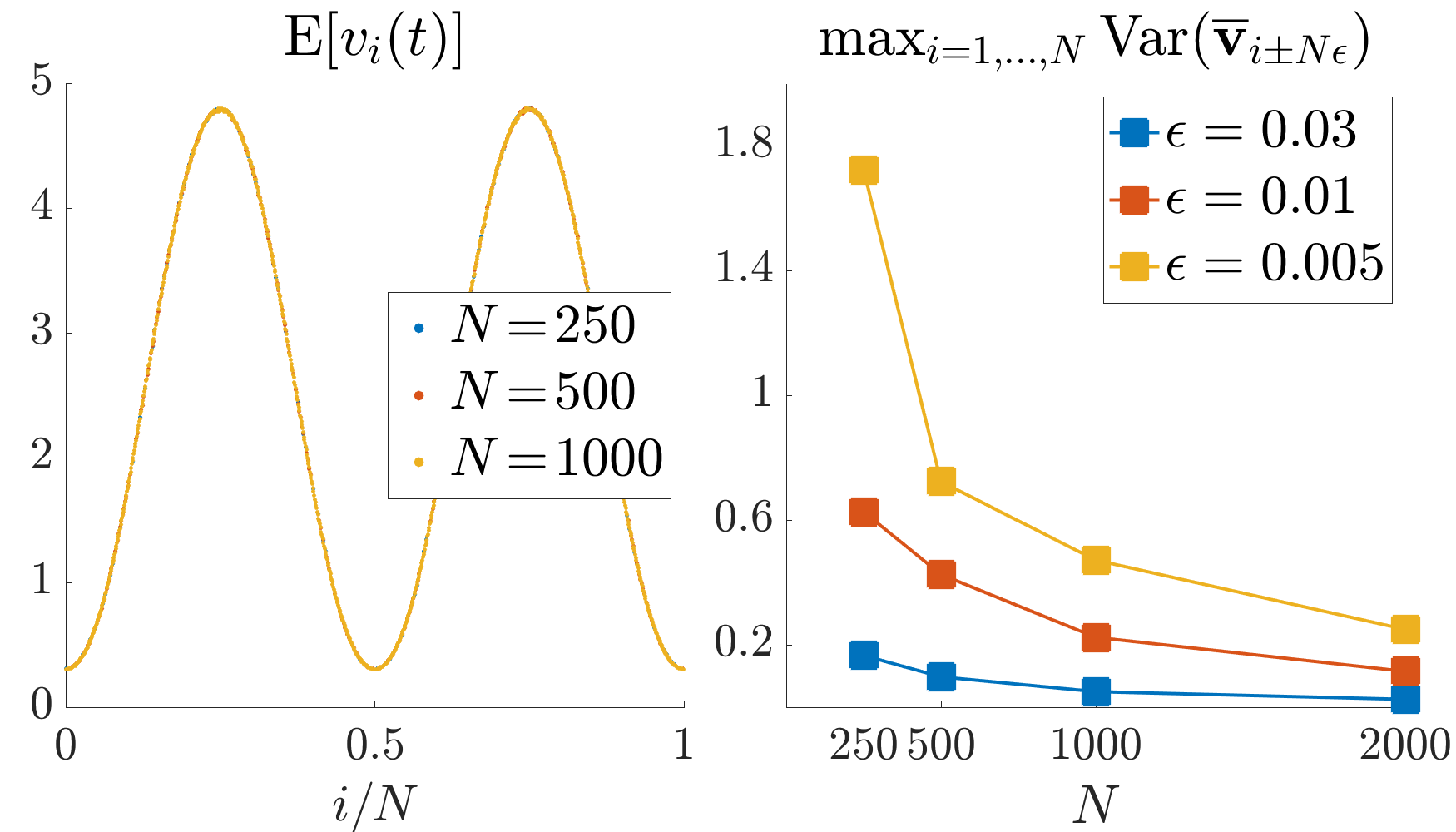
Using numerical simulation, one can get much stronger results. Indeed, we show that the symmetric nearest neighbor zero range process has a smooth LE state, i.e. it satisfies (V), (E\,{}^{\prime}), and (Ef\,{}^{\prime}). For the rate function g𝑔g of the zero range process, we take g(k)=k+k1/4𝑔𝑘𝑘superscript𝑘14g(k)=k+k^{1/4}. The reason for this choice of g𝑔g is that it satisfies the condition of linear growth, assumed in the proof of (28) given in [12]. Moreover, we choose g𝑔g to be nonlinear, in order to make the existence of g^^𝑔\hat{g} nontrivial (when verifying (Ef\,{}^{\prime}) with f=g𝑓𝑔f=g). For our initial macroscopic condition we take v0(x)=5sin(2πx)2v_{0}(x)=5\sin(2\pi x)^{2}. See Appendix B.1 for the details of the numerical simulations. The left panel of Figure 2 depicts the i/N𝔼[vi(t)]maps-to𝑖𝑁𝔼delimited-[]subscript𝑣𝑖𝑡i/N\mapsto\mathbb{E}\,[v_{i}(t)] profile, and the right panel depicts maxiVar(𝐯¯i±Nϵ)subscript𝑖Varsubscript¯𝐯plus-or-minus𝑖𝑁italic-ϵ\max_{i}\mathrm{Var}(\overline{\bf v}_{i\pm N\epsilon}), for N=500,1000,2000𝑁50010002000N=500,1000,2000.

Refer to caption
Figure 2: Verification of (E\,{}^{\prime}) and (V). For each N𝑁N, the expectations 𝔼[vi(t)]𝔼delimited-[]subscript𝑣𝑖𝑡\mathbb{E}\,[v_{i}(t)] and variances Var(𝐯¯i±Nϵ)Varsubscript¯𝐯plus-or-minus𝑖𝑁italic-ϵ\mathrm{Var}(\overline{\bf v}_{i\pm N\epsilon}) are estimated from an average of 2×1052superscript1052\times 10^{5} samples.

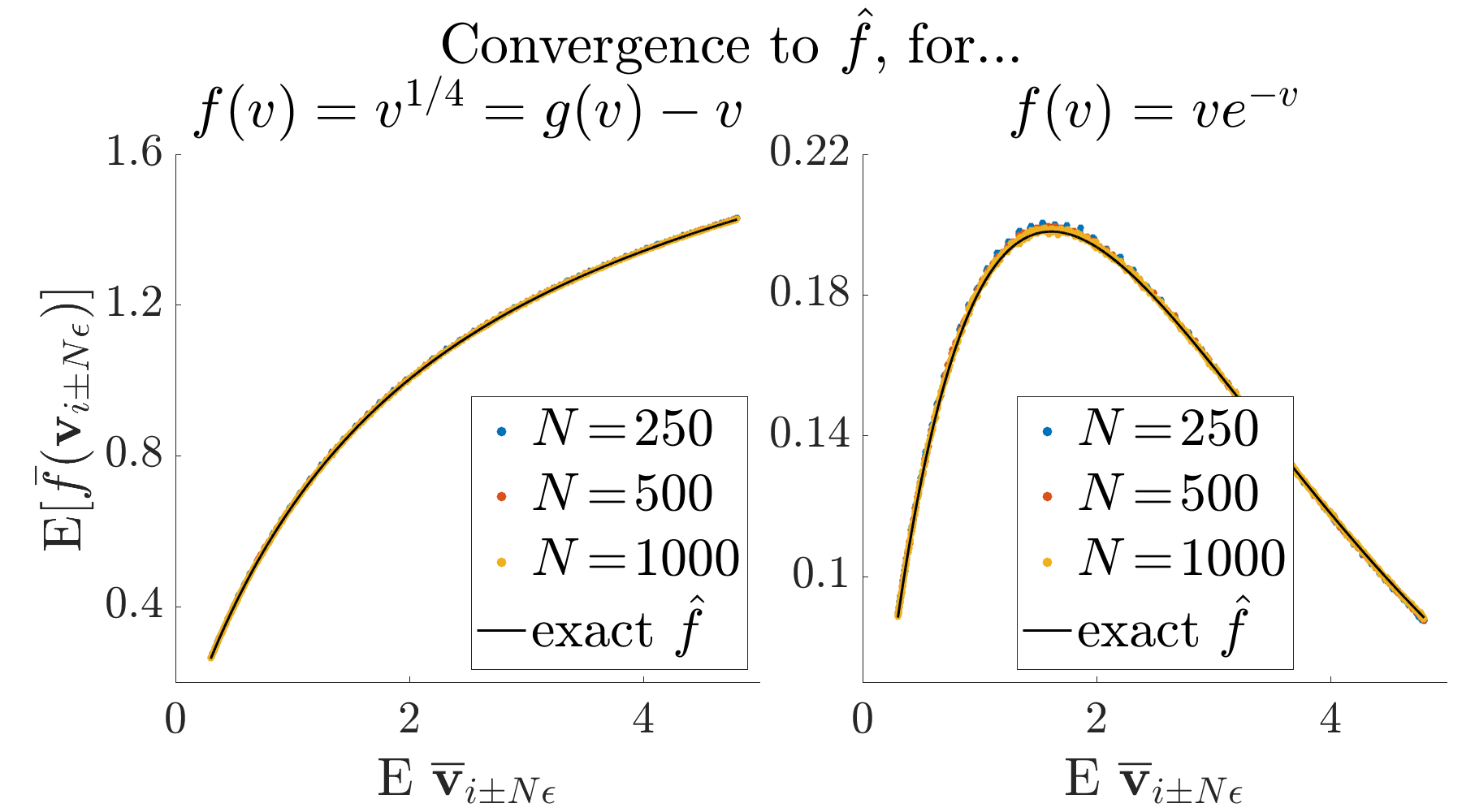
It is clear from the left panel that there is a smooth function v(t,x)𝑣𝑡𝑥v(t,x) such that 𝔼[vNx+R(t)]𝔼delimited-[]subscript𝑣𝑁𝑥𝑅𝑡\mathbb{E}\,[v_{Nx+R}(t)] converges to v(t,x)𝑣𝑡𝑥v(t,x) as N𝑁N\to\infty for any fixed R𝑅R. This confirms (E\,{}^{\prime}). The right panel also clearly confirms (V). Next, we verify (Ef\,{}^{\prime}) for two functions f𝑓f: f(v)=g(v)v=v1/4𝑓𝑣𝑔𝑣𝑣superscript𝑣14f(v)=g(v)-v=v^{1/4}, where g𝑔g is the rate function, and f(v)=vev𝑓𝑣𝑣superscript𝑒𝑣f(v)=ve^{-v}. To check that this limit holds, we plot pairs (𝔼vi,𝔼f(vi))𝔼subscript𝑣𝑖𝔼𝑓subscript𝑣𝑖(\mathbb{E}\,v_{i},\mathbb{E}\,f(v_{i})) to see if they line up on the curve (v,f^(v))𝑣^𝑓𝑣(v,\hat{f}(v)) as N𝑁N increases. This is shown in Figure 3. The function f^^𝑓\hat{f} is computed explicitly using our explicit knowledge of μ[]𝜇delimited-[]\mu[\cdot]. See Appendix A for the details.

Refer to caption
Figure 3: Verification of (Ef\,{}^{\prime}) for two functions f𝑓f.

4.4 Hard Core Exclusion; Crystal Slope Process

We confirm the distinguishing feature of smooth LEs, that 𝔼[vi(t)]𝔼delimited-[]subscript𝑣𝑖𝑡\mathbb{E}\,[v_{i}(t)] varies smoothly across lattice sites i𝑖i, for two more processes. First, we simulate a hard core exclusion process satisfying the conditions of [4]. Under these conditions, the authors prove that Law(𝐯N(t))μv(t,)NLawsubscript𝐯𝑁𝑡subscriptsuperscript𝜇𝑁𝑣𝑡{\mathrm{Law}}(\mathbf{v}_{N}(t))\approx\mu^{N}_{v(t,\cdot)}, where μv(t,)Nsubscriptsuperscript𝜇𝑁𝑣𝑡\mu^{N}_{v(t,\cdot)} takes the form (25) and μ[v]=Bernoulli(v)𝜇delimited-[]𝑣Bernoulli𝑣\mu[v]=\mathrm{Bernoulli}(v). See the paper for the precise statement which, as for the zero range process, is insufficient to show that the limits (E\,{}^{\prime}) or (Ef\,{}^{\prime}) hold. The plot of 𝔼vi𝔼subscript𝑣𝑖\mathbb{E}\,v_{i}, which we omit for brevity, clearly shows the 𝔼vi𝔼subscript𝑣𝑖\mathbb{E}\,v_{i} are smoothly varying.

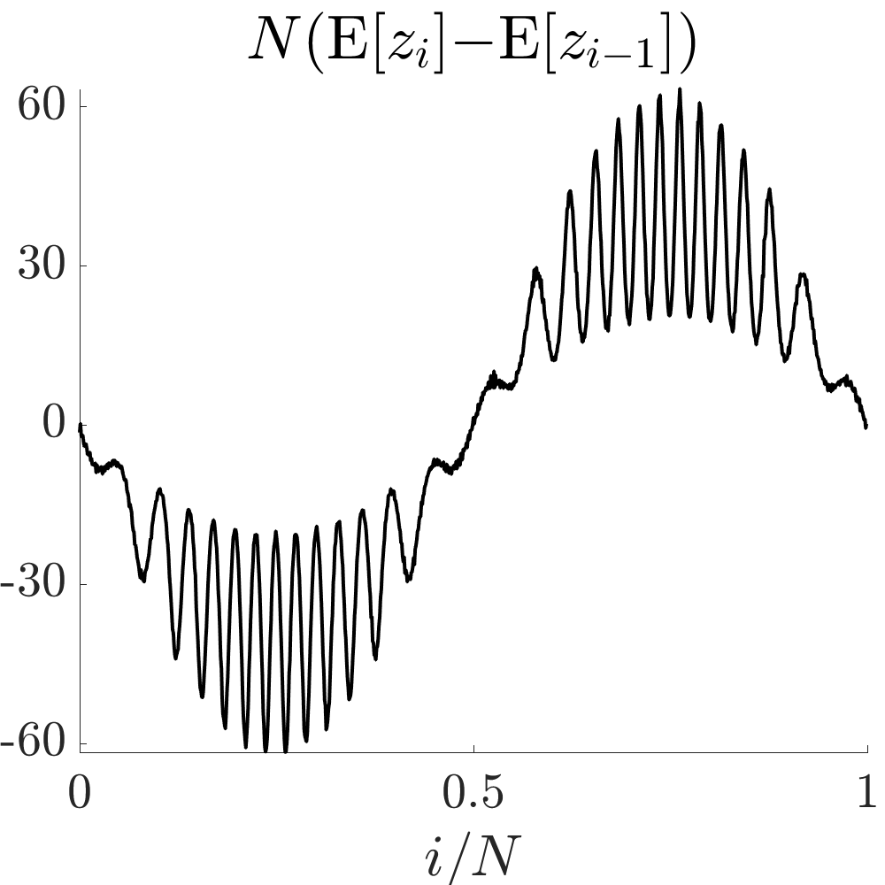
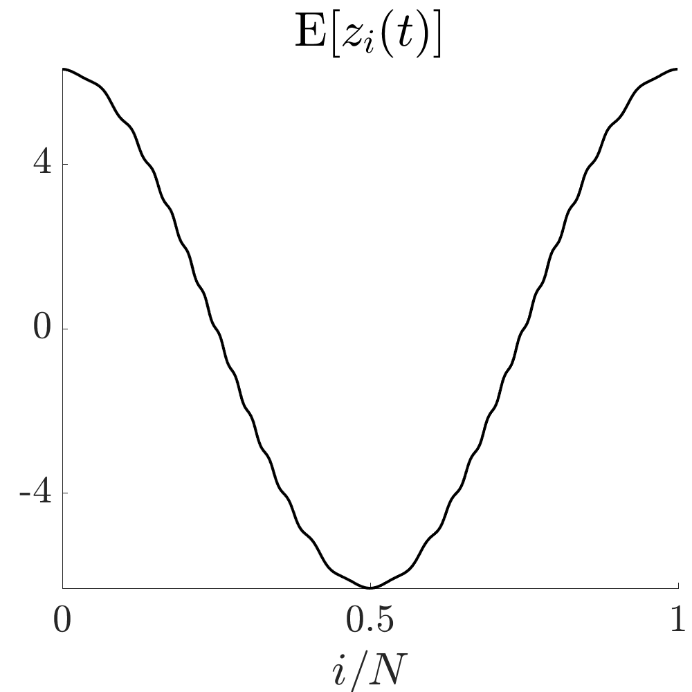
Second, we consider the crystal slope process in the smooth scaling regime, i.e. we take 𝐳N(t)=𝐳~N(N4t)subscript𝐳𝑁𝑡subscript~𝐳𝑁superscript𝑁4𝑡\mathbf{z}_{N}(t)=\tilde{\mathbf{z}}_{N}(N^{4}t), where zi=hi+1hisubscript𝑧𝑖subscript𝑖1subscript𝑖z_{i}=h_{i+1}-h_{i} for a height process initialized with amplitude scaling N1superscript𝑁1N^{1}. For this process, there are currently no rigorous results on the form of Law(𝐳N)Lawsubscript𝐳𝑁{\mathrm{Law}}(\mathbf{z}_{N}). However, as argued in [17], 𝐳Nsubscript𝐳𝑁\mathbf{z}_{N} is expected to have a smoothly varying local Gibbs LE state (for more on the local Gibbs distribution, see Section 6.1). The left and right panels of Figure 4 show 𝔼[zi(t)]𝔼delimited-[]subscript𝑧𝑖𝑡\mathbb{E}\,[z_{i}(t)] and N(𝔼[zi(t)]𝔼[zi1(t)])𝑁𝔼delimited-[]subscript𝑧𝑖𝑡𝔼delimited-[]subscript𝑧𝑖1𝑡N(\mathbb{E}\,[z_{i}(t)]-\mathbb{E}\,[z_{i-1}(t)]), respectively, as functions of i/N𝑖𝑁i/N. We take N=1000𝑁1000N=1000 and t=108𝑡superscript108t=10^{-8}. As expected, we see that 𝔼[zi(t)]𝔼delimited-[]subscript𝑧𝑖𝑡\mathbb{E}\,[z_{i}(t)] look smoothly varying, and interestingly, so do the finite differences. The oscillations in both plots are smooth, and not an artifact. They are a consequence of the function λDsubscript𝜆𝐷\lambda_{D} appearing in the PDE (for a plot of this function, see Figure 12).
Refer to caption
Refer to caption
Figure 4: Left: 𝔼[zi(t)]𝔼delimited-[]subscript𝑧𝑖𝑡\mathbb{E}\,[z_{i}(t)], for the time-rescaled crystal slope process in the smooth scaling regime. Right: N(𝔼[zi(t)]𝔼[zi1(t)])𝑁𝔼delimited-[]subscript𝑧𝑖𝑡𝔼delimited-[]subscript𝑧𝑖1𝑡N(\mathbb{E}\,[z_{i}(t)]-\mathbb{E}\,[z_{i-1}(t)]). Both seem to be smoothly varying. The oscillations are not an artifact; they are a result of the function λDsubscript𝜆𝐷\lambda_{D} appearing in the PDE. N=1000𝑁1000N=1000 and t=108𝑡superscript108t=10^{-8}.

5 Rough Local Equilibrium: A Numerical Study

We now return to the crystal process 𝐰Nsubscript𝐰𝑁\mathbf{w}_{N}. Our numerical study of the distribution of 𝐰N(t)subscript𝐰𝑁𝑡\mathbf{w}_{N}(t), starting in Section 5.2, will show that it is nothing like the prototypical LE state (25). However, we show in Section 5.3 that it is nevertheless a rough LE, satisfying (E), (Ef), and (V). Section 5.4 concludes with some qualitative observations. But first let us mention a few numerical considerations.

5.1 Numerical Considerations

Let 𝔼n[f(𝐰N(t))]superscript𝔼𝑛delimited-[]𝑓subscript𝐰𝑁𝑡\mathbb{E}\,^{n}[f(\mathbf{w}_{N}(t))] denote the average of
f(𝐰N(k)(t))𝑓superscriptsubscript𝐰𝑁𝑘𝑡f(\mathbf{w}_{N}^{(k)}(t)), k=1,,n𝑘1𝑛k=1,\dots,n, computed from n𝑛n independent runs of the process. We will also consider time averages

(29) 𝔼Δ[f(𝐰N(t))]:=1ΔIt𝔼[f(𝐰N(s))]𝑑s,assignsubscript𝔼Δdelimited-[]𝑓subscript𝐰𝑁𝑡1Δsubscriptsubscript𝐼𝑡𝔼delimited-[]𝑓subscript𝐰𝑁𝑠differential-d𝑠\begin{split}\mathbb{E}\,_{\Delta}[f(\mathbf{w}_{N}(t))]:=\frac{1}{\Delta}\int_{I_{t}}\mathbb{E}\,[f(\mathbf{w}_{N}(s))]ds,\end{split}

where Itsubscript𝐼𝑡I_{t} is any length ΔΔ\Delta interval containing t𝑡t. Let 𝔼Δn[f(𝐰N(t))]superscriptsubscript𝔼Δ𝑛delimited-[]𝑓subscript𝐰𝑁𝑡\mathbb{E}\,_{\Delta}^{n}[f(\mathbf{w}_{N}(t))] denote sample average estimates of 𝔼Δ[f(𝐰N(t))]subscript𝔼Δdelimited-[]𝑓subscript𝐰𝑁𝑡\mathbb{E}\,_{\Delta}[f(\mathbf{w}_{N}(t))]. For details on how we compute these quantities, see Appendix B.1.

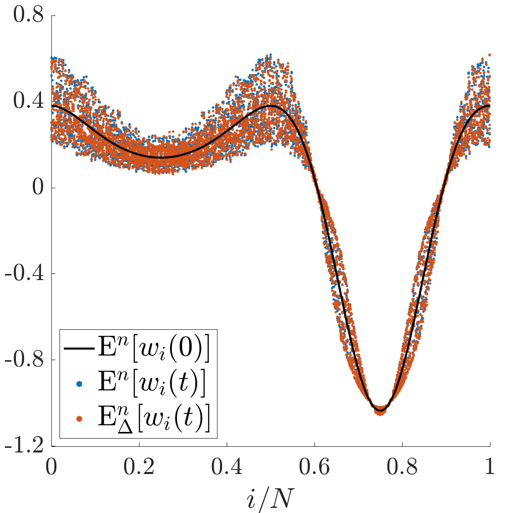
For precise confirmation of (E), (Ef), and (V), — which are statements about the instantaneous-time measure Law(𝐰N(t))Lawsubscript𝐰𝑁𝑡{\mathrm{Law}}(\mathbf{w}_{N}(t)) — we use the sample-only, instantaneous estimator 𝔼n[f(𝐰N(t))]superscript𝔼𝑛delimited-[]𝑓subscript𝐰𝑁𝑡\mathbb{E}\,^{n}[f(\mathbf{w}_{N}(t))]. The only exception is in computing the spatially averaged rate expectation 𝔼[r¯(𝐰N(x±ϵ))]𝔼delimited-[]¯𝑟subscript𝐰𝑁plus-or-minus𝑥italic-ϵ\mathbb{E}\,[\bar{r}({\bf w}_{N(x\pm\epsilon)})] needed to check (Ef) for f=r𝑓𝑟f=r. The rate observable has a very large variance (even upon spatial averaging) so we are forced to rely on the sample-and-time average (29), which has significantly lower variance. We justify our use of the time average to estimate the instantaneous-time rate expectation in Appendix B.2. We also use time averaging to compute expectations of other observables which help us understand additional properties of the LE state, which are not involved in our formal verification of (E), (Ef), and (V). In this case, it is simply convenient to have very low variance estimators since they give us a clearer picture of some qualitative features of the LE state. The left panel of Figure 5 shows that time averaging negligibly affects the 𝔼[wi(t)]𝔼delimited-[]subscript𝑤𝑖𝑡\mathbb{E}\,[w_{i}(t)] profile, and for other observables the discrepancy is also negligible. We will not further comment on time averaging, but we do indicate when we have time-averaged by writing 𝔼Δn[f(𝐰N(t)]\mathbb{E}\,^{n}_{\Delta}[f(\mathbf{w}_{N}(t)] in the plot titles.

We fix K=3𝐾3K=3 in all of the simulation results shown in this section.

5.2 No Smooth LE

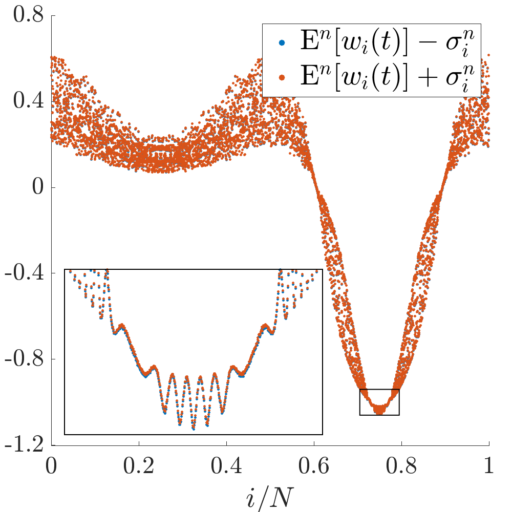
We begin by plotting i/N𝔼n[wi(t)]maps-to𝑖𝑁superscript𝔼𝑛delimited-[]subscript𝑤𝑖𝑡i/N\mapsto\mathbb{E}\,^{n}[w_{i}(t)] to show it is roughly varying, which automatically implies (E\,{}^{\prime}) is not satisfied. Consider Figure 5. The black line depicts the expectations 𝔼n[wi(0)]superscript𝔼𝑛delimited-[]subscript𝑤𝑖0\mathbb{E}\,^{n}[w_{i}(0)] at initialization, which are chosen so that 𝔼[wi(0)]=w0(i/N)𝔼delimited-[]subscript𝑤𝑖0subscript𝑤0𝑖𝑁\mathbb{E}\,[w_{i}(0)]=w_{0}(i/N) exactly. We take N=6000𝑁6000N=6000. Remarkably, in a time interval of macroscopic length t=2×10¹⁴𝑡2superscript1014t=2\times 10^{-14}, the process evolves from this smooth profile to the configuration shown by the blue dots, which are the points (i/N,𝔼n[wi(t)])𝑖𝑁superscript𝔼𝑛delimited-[]subscript𝑤𝑖𝑡(i/N,\mathbb{E}\,^{n}[w_{i}(t)]). We call these points a “cloud” rather than a curve, since they are so roughly varying that they do not seem to pass the straight line test. Interestingly, the cloud seems to narrows to a point at integer values of the range. This will be discussed in Section 6.2.

Due to the chaotic nature of the cloud in space, one might be led to believe that it is similarly chaotic in time. However, an interesting feature of the 𝔼n[wi(t)]superscript𝔼𝑛delimited-[]subscript𝑤𝑖𝑡\mathbb{E}\,^{n}[w_{i}(t)] process is that following a vanishingly small time tNsubscript𝑡𝑁t_{N}, the process evolves slowly. The red points in Figure 5 depict the values of the process averaged over the macroscopic time interval [1×1014,2×1014]1superscript10142superscript1014[1\times 10^{-14},2\times 10^{-14}]. We see that these red points, (i/N,𝔼Δn[wi(t)])𝑖𝑁subscriptsuperscript𝔼𝑛Δdelimited-[]subscript𝑤𝑖𝑡(i/N,\mathbb{E}\,^{n}_{\Delta}[w_{i}(t)]) are also roughly varying, and close to 𝔼n[wi(t)]superscript𝔼𝑛delimited-[]subscript𝑤𝑖𝑡\mathbb{E}\,^{n}[w_{i}(t)]. The fact that the chaotic cloud does not smooth out upon time averaging is a clear sign that it evolves slowly in time.
Refer to caption
Refer to caption
Figure 5: N=6000𝑁6000N=6000. Left: the roughly varying 𝔼n[wi(t)]superscript𝔼𝑛delimited-[]subscript𝑤𝑖𝑡\mathbb{E}\,^{n}[w_{i}(t)], and the time average thereof. Right: Profiles one standard deviation, denoted σnisubscriptsuperscript𝜎𝑖𝑛\sigma^{i}_{n}, away from the sample average 𝔼n[wi(t)]superscript𝔼𝑛delimited-[]subscript𝑤𝑖𝑡\mathbb{E}\,^{n}[w_{i}(t)], with n=106𝑛superscript106n=10^{6}.

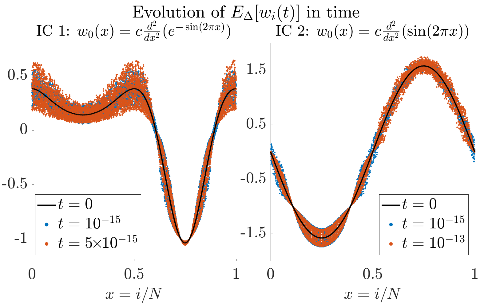
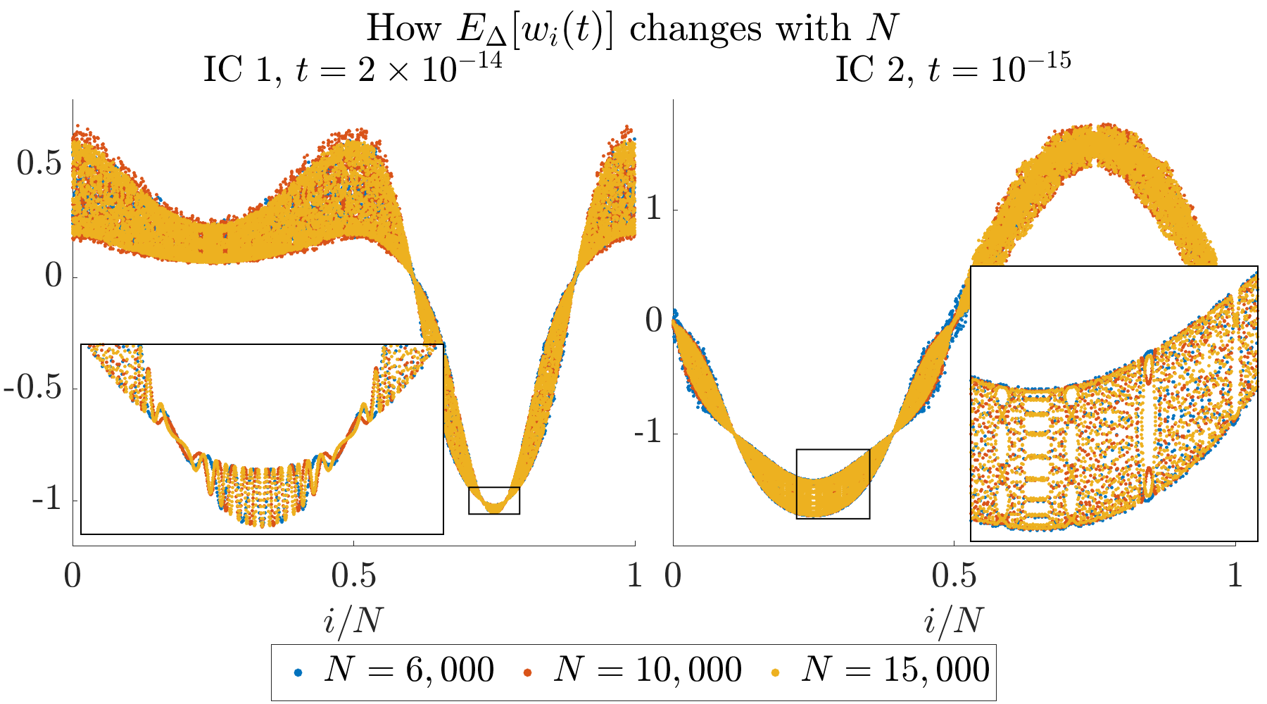
We offer three more tests to confirm that the i/N𝔼n[wi(t)]maps-to𝑖𝑁superscript𝔼𝑛delimited-[]subscript𝑤𝑖𝑡i/N\mapsto\mathbb{E}\,^{n}[w_{i}(t)] cloud is a real and “permanent” phenomenon. First, we show in the right panel of Figure 5 that the cloud is not due to randomness of the sample average approximation to 𝔼[wi(t)]𝔼delimited-[]subscript𝑤𝑖𝑡\mathbb{E}\,[w_{i}(t)]. The plot depicts a confidence interval of one standard deviation, denoted σinsuperscriptsubscript𝜎𝑖𝑛\sigma_{i}^{n}, around the sample mean 𝔼n[wi(t)]superscript𝔼𝑛delimited-[]subscript𝑤𝑖𝑡\mathbb{E}\,^{n}[w_{i}(t)], with n=106𝑛superscript106n=10^{6}. The second and third tests are to verify that the cloud persists in time and with increasing N𝑁N. Figure 6(a) depicts the evolution of 𝔼Δn[wi(t)]subscriptsuperscript𝔼𝑛Δdelimited-[]subscript𝑤𝑖𝑡\mathbb{E}\,^{n}_{\Delta}[w_{i}(t)] in time starting from two smooth initial conditions (ICs), which we call IC 1 and IC 2. They are denoted w0(x)=h0′′(x)subscript𝑤0𝑥superscriptsubscript0′′𝑥w_{0}(x)=h_{0}^{\prime\prime}(x) in the plot because we evolve forward the height process to get the curvature process. Clearly, the cloud persists in time for both ICs.
Refer to caption
(a) Evolution in time of 𝔼Δn[wi(t)]subscriptsuperscript𝔼𝑛Δdelimited-[]subscript𝑤𝑖𝑡\mathbb{E}\,^{n}_{\Delta}[w_{i}(t)] from two initial conditions.
Refer to caption
(b) Form of expectations 𝔼Δn[wi(t)]subscriptsuperscript𝔼𝑛Δdelimited-[]subscript𝑤𝑖𝑡\mathbb{E}\,^{n}_{\Delta}[w_{i}(t)] for several values of N𝑁N.

Meanwhile, Figure 6(b) confirms that the cloud persists with increasing N𝑁N, for both of these ICs. The figure also shows that 𝔼Δn[wi(t)]subscriptsuperscript𝔼𝑛Δdelimited-[]subscript𝑤𝑖𝑡\mathbb{E}\,^{n}_{\Delta}[w_{i}(t)] does not converge with N𝑁N. This is particularly evident in the insets.

The fact that 𝔼[wi]𝔼delimited-[]subscript𝑤𝑖\mathbb{E}\,[w_{i}] varies roughly does not rule out the possibility that the single site marginals Law(wi(t))Lawsubscript𝑤𝑖𝑡\mathrm{Law}(w_{i}(t)) belong to a mean-parameterized measure family. However, Figure 7 shows that (Ef\,{}^{\prime}) is not satisfied: there is no functionf^^𝑓\hat{f} taking 𝔼wi𝔼subscript𝑤𝑖\mathbb{E}\,w_{i} to 𝔼f(wi)𝔼𝑓subscript𝑤𝑖\mathbb{E}\,f(w_{i}) in the N𝑁N\to\infty limit. As a result, Law(wi(t))Lawsubscript𝑤𝑖𝑡\mathrm{Law}(w_{i}(t)) cannot belong to any mean-parameterized measure family.
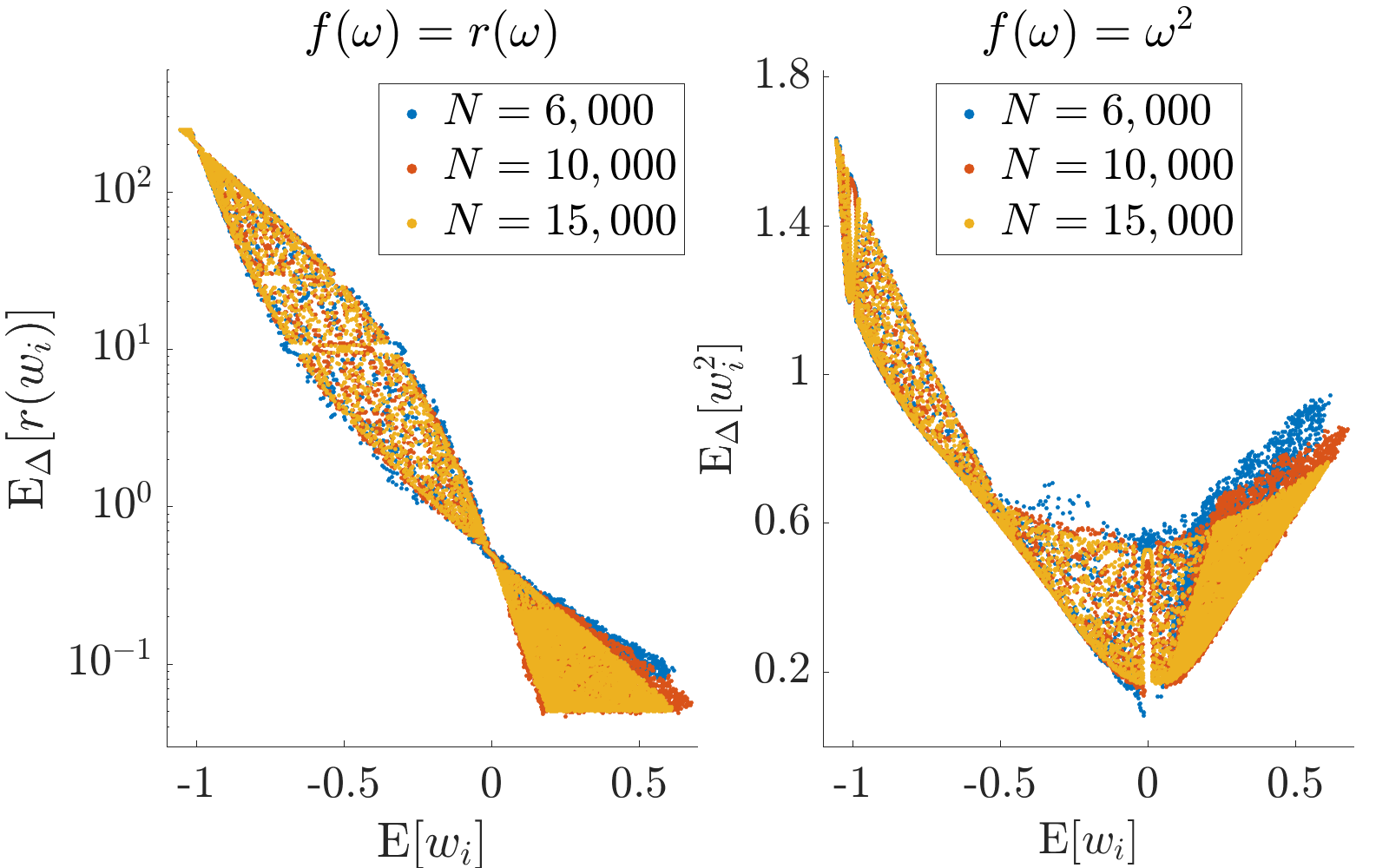
Refer to caption
Figure 7: There is no function f^^𝑓\hat{f} taking 𝔼wi𝔼subscript𝑤𝑖\mathbb{E}\,w_{i} to 𝔼f(wi)𝔼𝑓subscript𝑤𝑖\mathbb{E}\,f(w_{i}) in the N𝑁N\to\infty limit. Therefore, (Ef\,{}^{\prime}) is not satisfied, and Law(wi(t))Lawsubscript𝑤𝑖𝑡\mathrm{Law}(w_{i}(t)) cannot belong to any mean-parameterized measure family. Data shown from process generated by IC 1.

5.3 Verification of Rough LE

We now confirm the limits (V), (E), and (Ef) hold, and that the limit w(t,x)𝑤𝑡𝑥w(t,x) in (E) is continuous in x𝑥x. Figure 8 confirms (V). In fact, the figure shows that 1) the window average variances go to zero uniformly across the lattice, and 2) the second ϵ0italic-ϵ0\epsilon\to 0 limit is unnecessary. For the variance to go to zero, we simply need to average over increasingly large window sizes. Indeed, keeping ϵ>0italic-ϵ0\epsilon>0 fixed, the variance decays as the window size 2Nϵ2𝑁italic-ϵ2N\epsilon increases.

Refer to caption
Figure 8: Confirmation of (V). In fact, these plots suggest that the limit holds uniformly in x𝑥x. We also see that the outer ϵ0italic-ϵ0\epsilon\to 0 limit is unnecessary: for each fixed ϵ>0italic-ϵ0\epsilon>0, the variances decay as N𝑁N increases.

Next, we check (E). Doing so numerically is somewhat delicate, since for any finite N𝑁N, if we take ϵitalic-ϵ\epsilon small enough the window average 𝔼[𝐰¯N(x±ϵ)]𝔼delimited-[]subscript¯𝐰𝑁plus-or-minus𝑥italic-ϵ\mathbb{E}\,\left[\overline{\bf w}_{{N(x\pm\epsilon)}}\right] will necessarily revert back to being rough and non-converging. Since we cannot take N𝑁N\to\infty numerically, we use the following proxy for convergence as N,ϵ0formulae-sequence𝑁italic-ϵ0N\to\infty,\epsilon\to 0. For each N𝑁N, we choose a “good” ϵ(N)italic-ϵ𝑁\epsilon(N) (see details in Appendix B.3), and then check that 𝔼[𝐰¯N(x±ϵ(N))]𝔼delimited-[]subscript¯𝐰𝑁plus-or-minus𝑥italic-ϵ𝑁\mathbb{E}\,[\overline{\bf w}_{N(x\pm\epsilon(N))}] converges as N𝑁N\to\infty. Figure 9 confirms that this convergence indeed holds. The continuity of the limit is clear from the plot.
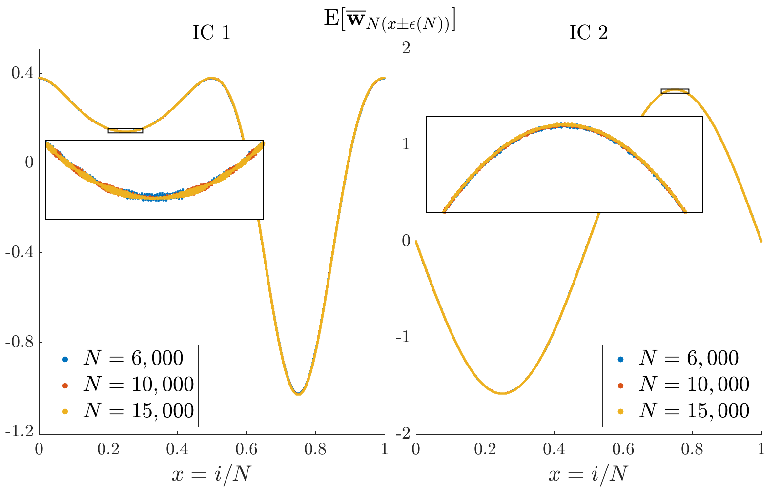
Refer to caption
Figure 9: Confirmation of (E). We take the limit by choosing a “good” ϵ(N)italic-ϵ𝑁\epsilon(N) for each N𝑁N, and taking N𝑁N\to\infty. For the procedure to choose ϵ(N)italic-ϵ𝑁\epsilon(N), see Appendix B.3.

Finally, let us check (Ef). If (Ef) holds, then for all initial conditions, for all i=1,,N𝑖1𝑁i=1,\dots,N, and for all t>0𝑡0t>0, the pairs (𝔼𝐰¯i±Nϵ,𝔼f¯(𝐰i±Nϵ))𝔼subscript¯𝐰plus-or-minus𝑖𝑁italic-ϵ𝔼¯𝑓subscript𝐰plus-or-minus𝑖𝑁italic-ϵ(\mathbb{E}\,\overline{\bf w}_{i\pm N\epsilon},\;\mathbb{E}\,\bar{f}({\bf w}_{i\pm N\epsilon})) should approximately lie on the curve {(ω,f^(ω)ω}\{(\omega,\hat{f}(\omega)\mid\omega\in\mathbb{R}\} for some function f^^𝑓\hat{f}. As N𝑁N increases and ϵitalic-ϵ\epsilon decreases, these points should adhere to this curve more closely. Figure 10 verifies (Ef) for f(ω)=r(ω)=e2K2Kω𝑓𝜔𝑟𝜔superscript𝑒2𝐾2𝐾𝜔f(\omega)=r(\omega)=e^{-2K-2K\omega} (the rate function), and f(ω)=ω2𝑓𝜔superscript𝜔2f(\omega)=\omega^{2}. As in the verification of (E), we choose an appropriate ϵ(N)italic-ϵ𝑁\epsilon(N) for each N𝑁N. To emphasize the universality of f^^𝑓\hat{f} across space, time, and initial conditions, we plot all the following points, for a given N𝑁N, in the same color:

{(𝔼𝐰¯i±Nϵ(k)(tk),𝔼f¯(𝐰i±Nϵ(k)(tk)))|i=1,,N;k=1,2},conditional-set𝔼subscriptsuperscript¯𝐰𝑘plus-or-minus𝑖𝑁italic-ϵsubscript𝑡𝑘𝔼¯𝑓subscriptsuperscript𝐰𝑘plus-or-minus𝑖𝑁italic-ϵsubscript𝑡𝑘formulae-sequence𝑖1𝑁𝑘12\left\{\bigg{(}\mathbb{E}\,\overline{\bf w}^{(k)}_{i\pm N\epsilon}(t_{k}),\;\mathbb{E}\,\bar{f}\big{(}{\bf w}^{(k)}_{i\pm N\epsilon}(t_{k})\big{)}\bigg{)}\;\bigg{|}\;i=1,\dots,N;\;k=1,2\right\},

where w(1)superscript𝑤1w^{(1)} and w(2)superscript𝑤2w^{(2)} denote the processes generated from ICs 1 and 2, respectively, and t1=2×10¹⁴subscript𝑡12superscript1014t_{1}=2\times 10^{-14}, t2=1015subscript𝑡2superscript1015t_{2}=10^{-15}.

Refer to caption
Figure 10: Confirmation of (Ef) for f(ω)=r(ω)𝑓𝜔𝑟𝜔f(\omega)=r(\omega) and f(ω)=ω2𝑓𝜔superscript𝜔2f(\omega)=\omega^{2}.

We see from the figure that as N𝑁N increases, the points corresponding to a given N𝑁N do in fact line up more closely on a single curve. Recall from Figure 7 that no universal function f^^𝑓\hat{f} sending 𝔼[wi]𝔼delimited-[]subscript𝑤𝑖\mathbb{E}\,[w_{i}] to 𝔼[f(wi)]𝔼delimited-[]𝑓subscript𝑤𝑖\mathbb{E}\,[f(w_{i})] exists. It is therefore remarkable that upon window averaging the domain and the range there does exist a universal function, i.e. which maps 𝔼𝐰¯i±Nϵ𝔼subscript¯𝐰plus-or-minus𝑖𝑁italic-ϵ\mathbb{E}\,\overline{\bf w}_{i\pm N\epsilon} to 𝔼f¯(𝐰i±Nϵ)𝔼¯𝑓subscript𝐰plus-or-minus𝑖𝑁italic-ϵ\mathbb{E}\,\bar{f}({\bf w}_{i\pm N\epsilon}).

Note that the points to the left of zero, i.e. for which 𝔼𝐰¯i±Nϵ<0𝔼subscript¯𝐰plus-or-minus𝑖𝑁italic-ϵ0\mathbb{E}\,\overline{\bf w}_{i\pm N\epsilon}<0, have lined up much more neatly on a single curve than points to the right of zero, for which 𝔼𝐰¯i±Nϵ>0𝔼subscript¯𝐰plus-or-minus𝑖𝑁italic-ϵ0\mathbb{E}\,\overline{\bf w}_{i\pm N\epsilon}>0. This indicates that the rate of LE onset, i.e. the rate at which the finite N𝑁N quantities in (V), (E), and (Ef) converge to their limits for a given time t𝑡t, is not uniform across x𝑥x. In particular, the rate of LE onset at a point x𝑥x seems to depend on the value of 𝔼𝐰¯N(x±ϵ)(t)𝔼subscript¯𝐰𝑁plus-or-minus𝑥italic-ϵ𝑡\mathbb{E}\,\overline{\bf w}_{{N(x\pm\epsilon)}}(t) (i.e. on the value of w(t,x)𝑤𝑡𝑥w(t,x), to which 𝔼𝐰¯N(x±ϵ)(t)𝔼subscript¯𝐰𝑁plus-or-minus𝑥italic-ϵ𝑡\mathbb{E}\,\overline{\bf w}_{{N(x\pm\epsilon)}}(t) converges). There is a straightforward informal explanation for this observation. It is intuitively clear that local equilibration (i.e. mixing) requires movement of particles, and there is little movement in regions where the rates are very small. From the left panel of Figure 10, we see that on average, the rates become exponentially smaller as 𝔼𝐰¯N(x±ϵ)𝔼subscript¯𝐰𝑁plus-or-minus𝑥italic-ϵ\mathbb{E}\,\overline{\bf w}_{{N(x\pm\epsilon)}} increases. Therefore, the larger the value of 𝔼𝐰¯N(x±ϵ)𝔼subscript¯𝐰𝑁plus-or-minus𝑥italic-ϵ\mathbb{E}\,\overline{\bf w}_{{N(x\pm\epsilon)}}, the slower the local equilibration.

5.4 Qualitative Study

We conclude the section with some further qualitative observations about the 𝐰Nsubscript𝐰𝑁\mathbf{w}_{N} process’s local equilibrium state, based on the form of i/N𝔼[fΔ(wi)]maps-to𝑖𝑁𝔼delimited-[]subscript𝑓Δsubscript𝑤𝑖i/N\mapsto\mathbb{E}\,[f_{\Delta}(w_{i})] profiles. Figure 11 depicts the expectations 𝔼Δ[wi]subscript𝔼Δdelimited-[]subscript𝑤𝑖\mathbb{E}\,_{\Delta}[w_{i}], 𝔼Δ[wi2]subscript𝔼Δdelimited-[]superscriptsubscript𝑤𝑖2\mathbb{E}\,_{\Delta}[w_{i}^{2}] and 𝔼Δ[r(wi)]subscript𝔼Δdelimited-[]𝑟subscript𝑤𝑖\mathbb{E}\,_{\Delta}[r(w_{i})] for the processes generated from the two ICs, and N=15,000𝑁15000N=15,000.

Refer to caption
Figure 11: Observable expectations

First, consider the bottom row, associated to IC 2. Note that for each of the three observables, there is a qualitative difference between the form of the profile in the region (0.6,0.9)0.60.9(0.6,0.9) (approximately) and the form elsewhere. For example, outside this region we observe that the (i/N,𝔼Δ[wi])𝑖𝑁subscript𝔼Δdelimited-[]subscript𝑤𝑖(i/N,\mathbb{E}\,_{\Delta}[w_{i}]) cloud narrows to a point when 𝔼Δ[wi]subscript𝔼Δdelimited-[]subscript𝑤𝑖\mathbb{E}\,_{\Delta}[w_{i}] takes the value 0 or -1 (an integer) But inside this region, the cloud does not narrow to a point near integer values of the range (i.e. where 𝔼Δ[wi]=1subscript𝔼Δdelimited-[]subscript𝑤𝑖1\mathbb{E}\,_{\Delta}[w_{i}]=1).

This has to do with the fact that the rate expectations in the region (0.6,0.9)0.60.9(0.6,0.9) are on the order of 104superscript10410^{-4}, which is extremely small relative to the largest rate expectation on the order of 104superscript10410^{4}. This is shown in the bottom rightmost panel. As we discussed above, we expect LE onset to be slowest where the rates are smallest, so the qualitative form of observable expectations in (0.6,0.9)0.60.9(0.6,0.9) is not characteristic of the LE state. Discounting this region for the second process, we make the following three observations about the form of these expectations.

  1. 1.

    The rate expectations 𝔼[r(wi)]𝔼delimited-[]𝑟subscript𝑤𝑖\mathbb{E}\,[r(w_{i})] are smoothly varying. This is not true of all observable expectations, since

  2. 2.

    The means 𝔼wi𝔼subscript𝑤𝑖\mathbb{E}\,w_{i} are roughly varying, as are the second moments.

  3. 3.

    The (i/N,𝔼wi)𝑖𝑁𝔼subscript𝑤𝑖(i/N,\mathbb{E}\,w_{i}) cloud narrows to a point near integer values of the range.

The smoothness of the rate expectations is surprising given that the first and second moments are so roughly varying. In the next section, we will give a partial explanation for this by showing that 𝔼[wi]𝔼delimited-[]subscript𝑤𝑖\mathbb{E}\,[w_{i}] are roughly varying because 𝔼[r(wi)]𝔼delimited-[]𝑟subscript𝑤𝑖\mathbb{E}\,[r(w_{i})] are smoothly varying. We will also explain the third observation.

In the present section, we gleaned useful information about the LE state by probing (V), (E) and (Ef) numerically, without ever referring to the explicit form of the distribution. In the next section, we will obtain a deeper understanding of the rough LE state using the explicit, limiting form of Law(wi)Lawsubscript𝑤𝑖\mathrm{Law}(w_{i}) (as confirmed by numerics, but without proof). Knowing the LE distribution explicitly is a rare privilege; for many interacting particle systems, there is no closed form expression for the LE state.

When the distribution is unknown, studying (V), (E), and (Ef) numerically is a useful tool to understand essential properties of the LE state. In fact, numerical simulations like the ones shown here can be used to derive the PDE limit for IPS in which the LE state, and therefore also the PDE, have no explicit analytic representation. We do this in [11] for a crystal surface dynamics with Metropolis-type rates.

6 A Look under the Hood at the Rough LE State

Although the previous section shows that the crucial limits (V), (E), and (Ef) are satisfied, several questions remain unresolved. The key question we address in this section is the following: given that Law(wi)Lawsubscript𝑤𝑖\mathrm{Law}(w_{i}) do not lie in a mean-parameterized measure family, where does the function

f^:𝔼𝐰¯i±Nϵ𝔼f¯(𝐰i±Nϵ):^𝑓maps-to𝔼subscript¯𝐰plus-or-minus𝑖𝑁italic-ϵ𝔼¯𝑓subscript𝐰plus-or-minus𝑖𝑁italic-ϵ\hat{f}:\mathbb{E}\,\overline{\bf w}_{i\pm N\epsilon}\mapsto\mathbb{E}\,\bar{f}({\bf w}_{i\pm N\epsilon})

come from? To answer this and other questions, we begin in Section 6.1 by writing down the form of Law(wi)Lawsubscript𝑤𝑖{\mathrm{Law}}(w_{i}) explicitly, and confirming this form numerically. At the end of 6.1, we summarize all assumptions used in the rigorous proofs in Sections 6.2 and 6.3. These include the numerically confirmed limit (E), and a slightly stronger version of what we can confirm numerically about Law(wi)Lawsubscript𝑤𝑖{\mathrm{Law}}(w_{i}). In Section 6.2, we rigorously prove further properties of the LE state using the assumptions. In particular, we address Observations 1,2,3 of Section 5.4, explaining how the intriguing shape of the i/N𝔼wimaps-to𝑖𝑁𝔼subscript𝑤𝑖i/N\mapsto\mathbb{E}\,w_{i} profile arises, and how this shape is related to the smoothness of the rate expectations. The heart of this section is 6.3, in which we rigorously prove that (Ef) is satisfied thanks to mesoscopic averaging of Law(wi)Lawsubscript𝑤𝑖{\mathrm{Law}}(w_{i}). We conclude in Section 6.4 by synthesizing how the rough LE arises, and how the rough LE affects the PDE limit.

6.1 The form of Law(𝐰N)subscript𝐰𝑁(\mathbf{w}_{N}), via Law(𝐳N)subscript𝐳𝑁(\mathbf{z}_{N})

Although we have been studying 𝐰Nsubscript𝐰𝑁\mathbf{w}_{N} independently of 𝐳Nsubscript𝐳𝑁\mathbf{z}_{N} and 𝐡Nsubscript𝐡𝑁\mathbf{h}_{N}, we will now reintroduce the 𝐳Nsubscript𝐳𝑁\mathbf{z}_{N} process. This will allow us to deduce the form of Law(𝐰N)Lawsubscript𝐰𝑁{\mathrm{Law}}(\mathbf{w}_{N}) from Law(𝐳N)Lawsubscript𝐳𝑁{\mathrm{Law}}(\mathbf{z}_{N}), which we know more about. Let 𝐳N(t)=(z1(t),,zN(t))subscript𝐳𝑁𝑡subscript𝑧1𝑡subscript𝑧𝑁𝑡\mathbf{z}_{N}(t)=(z_{1}(t),\dots,z_{N}(t)) be any process satisfying zi(t)zi1(t)=wi(t)subscript𝑧𝑖𝑡subscript𝑧𝑖1𝑡subscript𝑤𝑖𝑡z_{i}(t)-z_{i-1}(t)=w_{i}(t). This process 𝐳Nsubscript𝐳𝑁\mathbf{z}_{N} will have generator Nsubscript𝑁\mathcal{L}_{N} defined as in (5), but with 𝐰,𝐰i,j𝐰superscript𝐰𝑖𝑗\mathbf{w},\mathbf{w}^{i,j} replaced by 𝐳,𝐳i,j𝐳superscript𝐳𝑖𝑗\mathbf{z},\mathbf{z}^{i,j}, respectively. Recall from Section 2.1 that the ergodic invariant measures of the 𝐳Nsubscript𝐳𝑁\mathbf{z}_{N} process (i.e. the global equilibrium measures) take the form ΦN(𝐳izi=S0,iizi=S1)subscriptΦ𝑁formulae-sequenceconditional𝐳subscript𝑖subscript𝑧𝑖subscript𝑆0subscript𝑖𝑖subscript𝑧𝑖subscript𝑆1\Phi_{N}(\mathbf{z}\mid\sum_{i}z_{i}=S_{0},\sum_{i}iz_{i}=S_{1}), where ΦN(𝐳)eKH(𝐳)=exp(Ki=1Nzi2).proportional-tosubscriptΦ𝑁𝐳superscript𝑒𝐾𝐻𝐳exp𝐾superscriptsubscript𝑖1𝑁superscriptsubscript𝑧𝑖2\Phi_{N}({\bf z})\propto e^{-KH({\bf z})}=\,\mathrm{exp}(-K\sum_{i=1}^{N}z_{i}^{2}). By a conditional limit theorem, we should have

(30) ΦN(𝐳izi=S0,iizi=S1)1𝒵a0,a1exp(Kizi2+2Ka0izi+2Ka1iizi)subscriptΦ𝑁formulae-sequence𝐳subscript𝑖subscript𝑧𝑖subscript𝑆0subscript𝑖𝑖subscript𝑧𝑖subscript𝑆11subscript𝒵subscript𝑎0subscript𝑎1exp𝐾subscript𝑖superscriptsubscript𝑧𝑖22𝐾subscript𝑎0subscript𝑖subscript𝑧𝑖2𝐾subscript𝑎1subscript𝑖𝑖subscript𝑧𝑖\begin{split}\Phi_{N}(\mathbf{z}\mid&\sum_{i}z_{i}=S_{0},\sum_{i}iz_{i}=S_{1})\\ &\approx\frac{1}{\mathcal{Z}_{a_{0},a_{1}}}\,\mathrm{exp}\bigg{(}-K\sum_{i}z_{i}^{2}+2Ka_{0}\sum_{i}z_{i}+2Ka_{1}\sum_{i}iz_{i}\bigg{)}\end{split}

for N1much-greater-than𝑁1N\gg 1, where a0subscript𝑎0a_{0} and a1subscript𝑎1a_{1} are functions of S0subscript𝑆0S_{0} and S1subscript𝑆1S_{1}. Define the one-parameter family ρK[]subscript𝜌𝐾delimited-[]\rho_{K}[\cdot] by

(31) ρK[λ](n)=eK(nλ)2𝒵K(λ),𝒵K(λ)=m=eK(mλ)2.formulae-sequencesubscript𝜌𝐾delimited-[]𝜆𝑛superscript𝑒𝐾superscript𝑛𝜆2subscript𝒵𝐾𝜆subscript𝒵𝐾𝜆superscriptsubscript𝑚superscript𝑒𝐾superscript𝑚𝜆2\rho_{K}[\lambda](n)=\frac{e^{-K(n-\lambda)^{2}}}{\mathcal{Z}_{K}(\lambda)},\quad\quad\mathcal{Z}_{K}(\lambda)=\sum_{m=-\infty}^{\infty}e^{-K(m-\lambda)^{2}}.

By completing the square in the exponent in (30), we see that the measure on the second line takes the form ρ𝝀NN=i=1NρK[a0+ia1]\rho^{N}_{{\bm{\lambda}}_{N}}=\otimes_{i=1}^{N}\rho_{K}[a_{0}+ia_{1}]. Thus, in global equilibrium, the parameters λi=a0+ia1subscript𝜆𝑖subscript𝑎0𝑖subscript𝑎1\lambda_{i}=a_{0}+ia_{1} associated to zisubscript𝑧𝑖z_{i} form a single line, determined by the two global parameters a0subscript𝑎0a_{0} and a1subscript𝑎1a_{1}. In local equilibrium, we expect the distribution of 𝐳N(t)=𝐳~N(N4t)subscript𝐳𝑁𝑡subscript~𝐳𝑁superscript𝑁4𝑡\mathbf{z}_{N}(t)=\tilde{\mathbf{z}}_{N}(N^{4}t) to also take the form i=1NρK[λi]superscriptsubscripttensor-product𝑖1𝑁absentsubscript𝜌𝐾delimited-[]subscript𝜆𝑖\otimes_{i=1}^{N}\rho_{K}[\lambda_{i}], where λia0(x)+ia1(x)subscript𝜆𝑖subscript𝑎0𝑥𝑖subscript𝑎1𝑥\lambda_{i}\approx a_{0}(x)+ia_{1}(x) are linear in each mesoscopic region iN(x±ϵ)𝑖𝑁plus-or-minus𝑥italic-ϵi\in{N(x\pm\epsilon)}. We make the following conjecture which, for now, does not assume the λisubscript𝜆𝑖\lambda_{i} have any special structure.

Conjecture 6.1 (Unverified).

For each t𝑡t there exist 𝝀N(t)=(λ1(t),,λN(t))subscript𝝀𝑁𝑡subscript𝜆1𝑡subscript𝜆𝑁𝑡{\bm{\lambda}}_{N}(t)=(\lambda_{1}(t),\dots,\lambda_{N}(t)) such that as N𝑁N\to\infty, the below approximation becomes accurate with respect to some divergence (e.g. relative entropy):

(32) Law(𝐳N(t))ρ𝝀N(t)N(𝐳)i=1NρK[λi(t)](zi),N.formulae-sequenceLawsubscript𝐳𝑁𝑡subscriptsuperscript𝜌𝑁subscript𝝀𝑁𝑡𝐳proportional-tosuperscriptsubscriptproduct𝑖1𝑁subscript𝜌𝐾delimited-[]subscript𝜆𝑖𝑡subscript𝑧𝑖𝑁{\mathrm{Law}}(\mathbf{z}_{N}(t))\approx\rho^{N}_{{\bm{\lambda}}_{N}(t)}({\bf z})\propto\prod_{i=1}^{N}\rho_{K}[\lambda_{i}(t)](z_{i}),\quad N\to\infty.

Note that we can think of ρK[λ]subscript𝜌𝐾delimited-[]𝜆\rho_{K}[\lambda] as the discrete (integer-supported) version of the normal distribution 𝒩(λ,1/2K)𝒩𝜆12𝐾\mathcal{N}(\lambda,1/2K). Define

uD(λ)=m1(ρK[λ])=n=neK(nλ)2/𝒵K(λ)subscript𝑢𝐷𝜆subscript𝑚1subscript𝜌𝐾delimited-[]𝜆superscriptsubscript𝑛𝑛superscript𝑒𝐾superscript𝑛𝜆2subscript𝒵𝐾𝜆u_{D}(\lambda)=m_{1}(\rho_{K}[\lambda])=\sum_{n=-\infty}^{\infty}ne^{-K(n-\lambda)^{2}}\bigg{/}\mathcal{Z}_{K}(\lambda)

the first moment of ρK[λ]subscript𝜌𝐾delimited-[]𝜆\rho_{K}[\lambda], and let λD=uD1subscript𝜆𝐷superscriptsubscript𝑢𝐷1\lambda_{D}=u_{D}^{-1}. For comparison, we let uC(λ)=λsubscript𝑢𝐶𝜆𝜆u_{C}(\lambda)=\lambda, the first moment of the distribution 𝒩(λ,1/2K)𝒩𝜆12𝐾\mathcal{N}(\lambda,1/2K), and λC=uC1subscript𝜆𝐶superscriptsubscript𝑢𝐶1\lambda_{C}=u_{C}^{-1}, also the identity function.

Refer to caption
Figure 12: uD(λ)=m1(ρK[λ])subscript𝑢𝐷𝜆subscript𝑚1subscript𝜌𝐾delimited-[]𝜆u_{D}(\lambda)=m_{1}(\rho_{K}[\lambda]), and λD=uD1subscript𝜆𝐷superscriptsubscript𝑢𝐷1\lambda_{D}=u_{D}^{-1}, when K=5𝐾5K=5. The oscillations are due to the discreteness of the support of ρK[λ]subscript𝜌𝐾delimited-[]𝜆\rho_{K}[\lambda].

Figure 12 shows a plot of uD(λ)subscript𝑢𝐷𝜆u_{D}(\lambda) and λD(u)subscript𝜆𝐷𝑢\lambda_{D}(u). Both functions implicitly depend on K𝐾K. The oscillations of uDsubscript𝑢𝐷u_{D} and λDsubscript𝜆𝐷\lambda_{D} around the identity functions uCsubscript𝑢𝐶u_{C} and λCsubscript𝜆𝐶\lambda_{C} are a consequence of the restricted support of ρK[λ]subscript𝜌𝐾delimited-[]𝜆\rho_{K}[\lambda] (restricted compared to the continuous normal distribution).

We will now partially confirm that the 𝐰Nsubscript𝐰𝑁\mathbf{w}_{N} distribution induced by the conjectured 𝐳Nsubscript𝐳𝑁\mathbf{z}_{N} distribution (32) is correct. Since we are interested in 𝐰Nsubscript𝐰𝑁\mathbf{w}_{N} through the lens of (V), (E), and (Ef), we do not need to know the full, N𝑁N site distribution Law(𝐰N)Lawsubscript𝐰𝑁{\mathrm{Law}}(\mathbf{w}_{N}). Indeed, the limit (V) only depends on the two site distributions Law(wi,wj)Lawsubscript𝑤𝑖subscript𝑤𝑗{\mathrm{Law}}(w_{i},w_{j}) through Cov(wi,wj)Covsubscript𝑤𝑖subscript𝑤𝑗\mathrm{Cov}(w_{i},w_{j}), and the limits (E) and (Ef) only depend on the one site distributions Law(wi)Lawsubscript𝑤𝑖{\mathrm{Law}}(w_{i}) through 𝔼[wi]𝔼delimited-[]subscript𝑤𝑖\mathbb{E}\,[w_{i}], 𝔼[f(wi)]𝔼delimited-[]𝑓subscript𝑤𝑖\mathbb{E}\,[f(w_{i})].

That Law(𝐳N)Lawsubscript𝐳𝑁\mathrm{Law}(\mathbf{z}_{N}) is given by a product measure in the N𝑁N\to\infty limit implies that we should have Corr(wNx+i,wNx+i+k)0Corrsubscript𝑤𝑁𝑥𝑖subscript𝑤𝑁𝑥𝑖𝑘0\mathrm{Corr}(w_{Nx+i},w_{Nx+i+k})\to 0 as N𝑁N\to\infty for all i𝑖i and lag k2𝑘2k\geq 2. Figure 13 confirms the correlation decay: the plots depict max2k9|Corr(wNx,wNx+k)|subscript2𝑘9Corrsubscript𝑤𝑁𝑥subscript𝑤𝑁𝑥𝑘\max_{2\leq k\leq 9}\left|\mathrm{Corr}(w_{Nx},w_{Nx+k})\right| as a function of x=i/N𝑥𝑖𝑁x=i/N with increasing N𝑁N, for the two processes generated from IC 1 and IC 2. In addition to confirming the correlation structure predicted by (32), Figure 13 also shows that maxk2|Corr(wNx,wNx+k)|subscript𝑘2Corrsubscript𝑤𝑁𝑥subscript𝑤𝑁𝑥𝑘\max_{k\geq 2}\left|\mathrm{Corr}(w_{Nx},w_{Nx+k})\right| is a useful metric for the rate of convergence to LE with N𝑁N in different spatial regions. Indeed, in the left panel we see that for the IC 1 - generated process, the correlations are lowest in the region i/N(0.6,0.9)𝑖𝑁0.60.9i/N\in(0.6,0.9), where the rates are highest (the rates are shown in the upper rightmost panel in Figure 11). This is in line with the intuition that regions with large jump rates are expected to equilibrate more quickly. For IC 2, the correlations are lowest in the region i/N(0.1,0.4)𝑖𝑁0.10.4i/N\in(0.1,0.4), also where the rates are highest (shown in the lower rightmost panel in Figure 11).
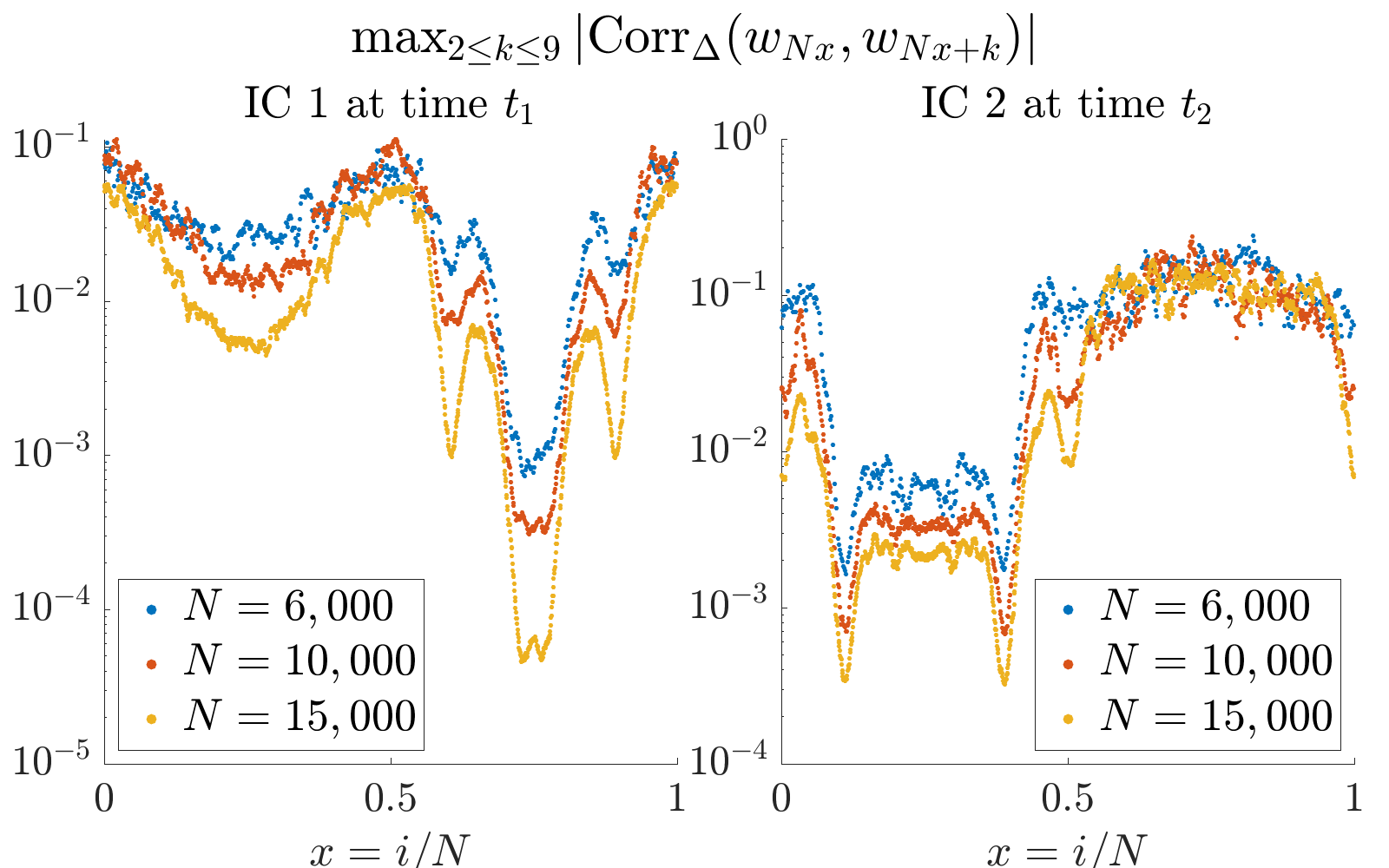
Refer to caption
Figure 13: Confirming that the correlations Corr(wi,wi+k)Corrsubscript𝑤𝑖subscript𝑤𝑖𝑘\mathrm{Corr}(w_{i},w_{i+k}) decay for all k2𝑘2k\geq 2, as predicted by (32). The figure also reveals that correlations are a useful metric for the rate of convergence of different spatial regions to LE.

This is all we have to say about pair distributions Law(wi,wi+k)Lawsubscript𝑤𝑖subscript𝑤𝑖𝑘{\mathrm{Law}}(w_{i},w_{i+k}). From now on, we are exclusively interested in Law(wi)Lawsubscript𝑤𝑖{\mathrm{Law}}(w_{i}).

Let μK[ω,λ]subscript𝜇𝐾𝜔𝜆\mu_{K}[\omega,\lambda] denote the distribution on ZZ𝑍superscript𝑍Z-Z^{\prime} induced by (Z,Z)ρK[λω]ρK[λ]similar-tosuperscript𝑍𝑍tensor-productsubscript𝜌𝐾delimited-[]𝜆𝜔subscript𝜌𝐾delimited-[]𝜆(Z^{\prime},Z)\sim\rho_{K}[\lambda-\omega]\otimes\rho_{K}[\lambda], so that

(33) Law(zi1,zi)ρK[λi1]ρK[λi]Law(wi)μK[ωi,λi],Lawsubscript𝑧𝑖1subscript𝑧𝑖tensor-productsubscript𝜌𝐾delimited-[]subscript𝜆𝑖1subscript𝜌𝐾delimited-[]subscript𝜆𝑖Lawsubscript𝑤𝑖subscript𝜇𝐾subscript𝜔𝑖subscript𝜆𝑖\begin{split}{\mathrm{Law}}(z_{i-1},z_{i})&\approx\rho_{K}[\lambda_{i-1}]\otimes\rho_{K}[\lambda_{i}]\\ \Rightarrow{\mathrm{Law}}(w_{i})&\approx\mu_{K}[\omega_{i},\lambda_{i}],\end{split}

where

ωi=λiλi1.subscript𝜔𝑖subscript𝜆𝑖subscript𝜆𝑖1\omega_{i}=\lambda_{i}-\lambda_{i-1}.

Note that if Zsuperscript𝑍Z^{\prime} and Z𝑍Z were independent continuous normals 𝒩(λω,1/2K)𝒩𝜆𝜔12𝐾\mathcal{N}(\lambda-\omega,1/2K) and 𝒩(λ,1/2K)𝒩𝜆12𝐾\mathcal{N}(\lambda,1/2K), then Law(ZZ)Law𝑍superscript𝑍{\mathrm{Law}}(Z-Z^{\prime}) would be 𝒩(ω,1/K)𝒩𝜔1𝐾\mathcal{N}(\omega,1/K), depending only on one parameter ω𝜔\omega (we are treating K𝐾K as fixed). However, due to the discreteness of the support of ρK[λ]subscript𝜌𝐾delimited-[]𝜆\rho_{K}[\lambda], the distribution μK[ω,λ]=Law(ZZ)subscript𝜇𝐾𝜔𝜆Law𝑍superscript𝑍\mu_{K}[\omega,\lambda]={\mathrm{Law}}(Z-Z^{\prime}) belongs to a two-parameter family, depending on both ω𝜔\omega and λ𝜆\lambda. We have

(34) μK[ω,λ](n)=(ZZ=n)=m=ρK[λω](m)ρK[λ](m+n)=m=exp(K(mλ+ω)2K(m+nλ)2)𝒵K(λω)𝒵K(λ)subscript𝜇𝐾𝜔𝜆𝑛𝑍superscript𝑍𝑛superscriptsubscript𝑚subscript𝜌𝐾delimited-[]𝜆𝜔𝑚subscript𝜌𝐾delimited-[]𝜆𝑚𝑛superscriptsubscript𝑚exp𝐾superscript𝑚𝜆𝜔2𝐾superscript𝑚𝑛𝜆2subscript𝒵𝐾𝜆𝜔subscript𝒵𝐾𝜆\begin{split}\mu_{K}[\omega,\lambda](n)&=\mathbb{P}(Z-Z^{\prime}=n)\\ &=\sum_{m=-\infty}^{\infty}\rho_{K}[\lambda-\omega](m)\rho_{K}[\lambda](m+n)\\ &=\sum_{m=-\infty}^{\infty}\frac{\,\mathrm{exp}\left(-K(m-\lambda+\omega)^{2}-K(m+n-\lambda)^{2}\right)}{\mathcal{Z}_{K}(\lambda-\omega)\mathcal{Z}_{K}(\lambda)}\end{split}

Expanding the squares and rearranging terms, we get

(35) μK[ω,λ](n)=exp(K2(nω)2)QK(n,ω,λ),subscript𝜇𝐾𝜔𝜆𝑛exp𝐾2superscript𝑛𝜔2subscript𝑄𝐾𝑛𝜔𝜆\begin{split}\mu_{K}[\omega,\lambda](n)=\,\mathrm{exp}\left(-\frac{K}{2}(n-\omega)^{2}\right)Q_{K}\left(n,\omega,\lambda\right),\end{split}

where

(36) QK(n,ω,λ)=𝒵2K(λ12[ω+n])𝒵K(λω)𝒵K(λ).subscript𝑄𝐾𝑛𝜔𝜆subscript𝒵2𝐾𝜆12delimited-[]𝜔𝑛subscript𝒵𝐾𝜆𝜔subscript𝒵𝐾𝜆Q_{K}\left(n,\omega,\lambda\right)=\frac{\mathcal{Z}_{2K}\bigg{(}\lambda-\frac{1}{2}\bigg{[}\omega+n\bigg{]}\bigg{)}}{\mathcal{Z}_{K}\big{(}\lambda-\omega\big{)}\mathcal{Z}_{K}\big{(}\lambda\big{)}}.

Note that QKsubscript𝑄𝐾Q_{K} depends on λ𝜆\lambda through λmod1modulo𝜆1\lambda\bmod 1, since the normalization constant functions 𝒵Ksubscript𝒵𝐾\mathcal{Z}_{K} and 𝒵2Ksubscript𝒵2𝐾\mathcal{Z}_{2K} are one-periodic. For the first moment of μK[ω,λ]subscript𝜇𝐾𝜔𝜆\mu_{K}[\omega,\lambda] we have

(37) m1(μK[ω,λ])=𝔼Z𝔼Z=uD(λ)uD(λω).subscript𝑚1subscript𝜇𝐾𝜔𝜆𝔼𝑍𝔼superscript𝑍subscript𝑢𝐷𝜆subscript𝑢𝐷𝜆𝜔m_{1}(\mu_{K}[\omega,\lambda])=\mathbb{E}\,Z-\mathbb{E}\,Z^{\prime}=u_{D}(\lambda)-u_{D}(\lambda-\omega).

This first moment depends in a non-trivial way on both ω𝜔\omega and λ𝜆\lambda, implying that in general, expectations of observables under this distribution are not functions of the first moment alone. The same was observed to be true of the wisubscript𝑤𝑖w_{i} in Figure 7 of Section 5.2: there is no function f^:𝔼wi𝔼[f(wi)]:^𝑓maps-to𝔼subscript𝑤𝑖𝔼delimited-[]𝑓subscript𝑤𝑖\hat{f}:\mathbb{E}\,w_{i}\mapsto\mathbb{E}\,[f(w_{i})], indicating that the wisubscript𝑤𝑖w_{i} are not mean-parameterized.

For future reference, let us also compute the rate expectation with respect to μK[ω,λ]subscript𝜇𝐾𝜔𝜆\mu_{K}[\omega,\lambda]. Recall that r(w)=e2K2Kw𝑟𝑤superscript𝑒2𝐾2𝐾𝑤r(w)=e^{-2K-2Kw}. Using that μK[ω,λ]=Law(ZZ)subscript𝜇𝐾𝜔𝜆Law𝑍superscript𝑍\mu_{K}[\omega,\lambda]={\mathrm{Law}}(Z-Z^{\prime}) where (Z,Z)ρK[λω]ρK[λ]similar-tosuperscript𝑍𝑍tensor-productsubscript𝜌𝐾delimited-[]𝜆𝜔subscript𝜌𝐾delimited-[]𝜆(Z^{\prime},Z)\sim\rho_{K}[\lambda-\omega]\otimes\rho_{K}[\lambda], we get

(38) μK[ω,λ](r)=e2K𝔼[e2KZ]𝔼[e2KZ].subscript𝜇𝐾𝜔𝜆𝑟superscript𝑒2𝐾𝔼delimited-[]superscript𝑒2𝐾superscript𝑍𝔼delimited-[]superscript𝑒2𝐾𝑍\begin{split}\mu_{K}[\omega,\lambda](r)=e^{-2K}\mathbb{E}\,\left[e^{2KZ^{\prime}}\right]\mathbb{E}\,\left[e^{-2KZ}\right].\end{split}

Now, we compute

(39) 𝔼ZρK[λ]exp(cKZ)=nexp(cKn)exp(K(nλ)2)𝒵K(λ)=exp(cKλ+c2K/4)nexp(K(nλc/2)2)𝒵K(λ)=exp(cKλ+c2K/4)𝒵K(λ+c/2)𝒵K(λ).subscript𝔼similar-to𝑍subscript𝜌𝐾delimited-[]𝜆exp𝑐𝐾𝑍subscript𝑛exp𝑐𝐾𝑛exp𝐾superscript𝑛𝜆2subscript𝒵𝐾𝜆exp𝑐𝐾𝜆superscript𝑐2𝐾4subscript𝑛exp𝐾superscript𝑛𝜆𝑐22subscript𝒵𝐾𝜆exp𝑐𝐾𝜆superscript𝑐2𝐾4subscript𝒵𝐾𝜆𝑐2subscript𝒵𝐾𝜆\begin{split}\mathbb{E}\,_{Z\sim\rho_{K}[\lambda]}\,\mathrm{exp}\left(cKZ\right)&=\frac{\sum_{n}\,\mathrm{exp}\left(cKn\right)\,\mathrm{exp}\left(-K(n-\lambda)^{2}\right)}{\mathcal{Z}_{K}(\lambda)}\\ &=\,\mathrm{exp}\left(cK\lambda+c^{2}K/4\right)\frac{\sum_{n}\,\mathrm{exp}\left(-K(n-\lambda-c/2)^{2}\right)}{\mathcal{Z}_{K}(\lambda)}\\ &=\,\mathrm{exp}\left(cK\lambda+c^{2}K/4\right)\frac{\mathcal{Z}_{K}(\lambda+c/2)}{\mathcal{Z}_{K}(\lambda)}.\end{split}

𝒵K(λ)subscript𝒵𝐾𝜆\mathcal{Z}_{K}(\lambda) has period 1, so when c𝑐c is an even integer, the ratio of 𝒵Ksubscript𝒵𝐾\mathcal{Z}_{K}’s is equal to 1. Using (39) in (38) with c=±2𝑐plus-or-minus2c=\pm 2, we get

(40) μK[ω,λ](r)=e2Kexp(K+2K(λω))exp(K2Kλ)=exp(2Kω).subscript𝜇𝐾𝜔𝜆𝑟superscript𝑒2𝐾exp𝐾2𝐾𝜆𝜔exp𝐾2𝐾𝜆exp2𝐾𝜔\begin{split}\mu_{K}[\omega,\lambda](r)=e^{-2K}\,\mathrm{exp}\left(K+2K(\lambda-\omega)\right)\,\mathrm{exp}\left(K-2K\lambda\right)=\,\mathrm{exp}\left(-2K\omega\right).\end{split}

We see that the rate observable has the rare property that its expectation with respect to μK[ω,λ]subscript𝜇𝐾𝜔𝜆\mu_{K}[\omega,\lambda] does not depend on λ𝜆\lambda! We return to this point later on.

We will now show numerically that indeed, there exist λ1,,λNsubscript𝜆1subscript𝜆𝑁\lambda_{1},\dots,\lambda_{N} such that the approximation Law(wi)μK[ωi,λi]Lawsubscript𝑤𝑖subscript𝜇𝐾subscript𝜔𝑖subscript𝜆𝑖{\mathrm{Law}}(w_{i})\approx\mu_{K}[\omega_{i},\lambda_{i}] becomes increasingly accurate in the limit. This will be sufficient for our analysis, and we will not need that Law(zi1,zi)ρK[λi1]ρK[λi]Lawsubscript𝑧𝑖1subscript𝑧𝑖tensor-productsubscript𝜌𝐾delimited-[]subscript𝜆𝑖1subscript𝜌𝐾delimited-[]subscript𝜆𝑖{\mathrm{Law}}(z_{i-1},z_{i})\approx\rho_{K}[\lambda_{i-1}]\otimes\rho_{K}[\lambda_{i}]. Note that in the above calculations, it was convenient to use the representation μK[ω,λ]=Law(ZZ)subscript𝜇𝐾𝜔𝜆Law𝑍superscript𝑍\mu_{K}[\omega,\lambda]={\mathrm{Law}}(Z-Z^{\prime}) for (Z,Z)ρK[λω]ρK[λ]similar-tosuperscript𝑍𝑍tensor-productsubscript𝜌𝐾delimited-[]𝜆𝜔subscript𝜌𝐾delimited-[]𝜆(Z^{\prime},Z)\sim\rho_{K}[\lambda-\omega]\otimes\rho_{K}[\lambda] to compute the rate expectation μK[ω,λ](r)subscript𝜇𝐾𝜔𝜆𝑟\mu_{K}[\omega,\lambda](r) and first moment m1(μK[ω,λ])subscript𝑚1subscript𝜇𝐾𝜔𝜆m_{1}(\mu_{K}[\omega,\lambda]). However, we could have also used the pmf (35) to do these computations. The following properties summarize our numerical findings, which include a crucial observation regarding the smoothness of the ωisubscript𝜔𝑖\omega_{i}.

Numerically Verified Properties 1.

There exist λ1,,λNsubscript𝜆1subscript𝜆𝑁\lambda_{1},\dots,\lambda_{N} such that…

  • 1.1

    The following limit holds:

    maxi=1,,NH(Law(wi)|μK[ωi,λi])0,N,formulae-sequencesubscript𝑖1𝑁𝐻conditionalLawsubscript𝑤𝑖subscript𝜇𝐾subscript𝜔𝑖subscript𝜆𝑖0𝑁\max_{i=1,\dots,N}H\bigg{(}\mathrm{Law}(w_{i})\,\bigg{|}\,\mu_{K}[\omega_{i},\lambda_{i}]\bigg{)}\to 0,\quad N\to\infty,

    where ωi=λiλi1subscript𝜔𝑖subscript𝜆𝑖subscript𝜆𝑖1\omega_{i}=\lambda_{i}-\lambda_{i-1} and μK[ω,λ]subscript𝜇𝐾𝜔𝜆\mu_{K}[\omega,\lambda] is the pmf defined in (35).

  • 1.2

    The ωisubscript𝜔𝑖\omega_{i} vary smoothly in the neighborhood of any x𝑥x (recall Definition 4.3). In fact, they satisfy the stronger property that for each t,x𝑡𝑥t,x, we have

    limϵ0¯limN¯maxiN(x±ϵ)N|ωi+1ωi|<C=C(t,x)<.¯subscriptitalic-ϵ0¯subscript𝑁subscript𝑖𝑁plus-or-minus𝑥italic-ϵ𝑁subscript𝜔𝑖1subscript𝜔𝑖𝐶𝐶𝑡𝑥\overline{\lim_{\epsilon\to 0}}\;\overline{\lim_{N\to\infty}}\max_{{i\in{N(x\pm\epsilon)}}}N|\omega_{i+1}-\omega_{i}|<C=C(t,x)<\infty.

Note that the smoothness of ωisubscript𝜔𝑖\omega_{i} is in line with the claim above Conjecture 6.1, that in mesoscopic regions around x𝑥x we can make the approximation λi=a0(x)+ia1(x)subscript𝜆𝑖subscript𝑎0𝑥𝑖subscript𝑎1𝑥\lambda_{i}=a_{0}(x)+ia_{1}(x). Figure 14 verifies these two properties numerically for the process generated from IC 1. For the details of how we found the λisubscript𝜆𝑖\lambda_{i}, see Appendix B.4 and Remark 6.7.

Refer to caption
Figure 14: Numerical Verification of Properties 1.1 and 1.2. For the details of how we found the λisubscript𝜆𝑖\lambda_{i}, see Appendix B.4. The KL divergences are computed based on 1000 samples. The plot on the right confirms that the limit N(ωiωi1)𝑁subscript𝜔𝑖subscript𝜔𝑖1N(\omega_{i}-\omega_{i-1}) exists as N𝑁N\to\infty, for i/N𝑖𝑁i/N in the most equilibrated region (0.6,0.9)0.60.9(0.6,0.9).

Note that the KL divergence is lowest for i/N(0.6,0.9)𝑖𝑁0.60.9i/N\in(0.6,0.9), which we identified as the region which is quickest to equilibrate, based on the correlation plot Figure 13 and the rate expectation plot in Figure 11. The smoothness of the ωisubscript𝜔𝑖\omega_{i} is very sensitive to LE onset, so we are only able to show Property 2 for x(0.6,0.9)𝑥0.60.9x\in(0.6,0.9).

We will use these numerical results in Section 6.2 to explain Observations 1-3 (made at the end of Section 5.4), and in Section 6.3 to explain why (Ef) is satisfied. For the sake of a clear presentation, let us list all the facts we will assume to be true from now on. Assumption 2.1 below is a stronger version of the numerically verified Property 1.1. Assumption 2.2 is the same as Property 2.2. The third assumption is that (E) holds, which was shown numerically in Section 5.3.

Assumptions 2.

.

  • 2.1

    For some N0subscript𝑁0N_{0}, and all N>N0𝑁subscript𝑁0N>N_{0}, there exist λisubscript𝜆𝑖\lambda_{i}, i=1,,N𝑖1𝑁i=1,\dots,N such that

    Law(wi)=μK[ωi,λi]i=1,,N,formulae-sequenceLawsubscript𝑤𝑖subscript𝜇𝐾subscript𝜔𝑖subscript𝜆𝑖for-all𝑖1𝑁\mathrm{Law}\big{(}w_{i}\big{)}=\mu_{K}[\omega_{i},\lambda_{i}]\quad\forall i=1,\dots,N,

    where ωi:=λiλi1assignsubscript𝜔𝑖subscript𝜆𝑖subscript𝜆𝑖1\omega_{i}:=\lambda_{i}-\lambda_{i-1} and μK[ω,λ]subscript𝜇𝐾𝜔𝜆\mu_{K}[\omega,\lambda] is the pmf defined in (35).

  • 2.2

    The ωisubscript𝜔𝑖\omega_{i} satisfy

    limϵ0¯limN¯maxiN(x±ϵ)N|ωi+1ωi|<C.¯subscriptitalic-ϵ0¯subscript𝑁subscript𝑖𝑁plus-or-minus𝑥italic-ϵ𝑁subscript𝜔𝑖1subscript𝜔𝑖𝐶\overline{\lim_{\epsilon\to 0}}\;\overline{\lim_{N\to\infty}}\max_{{i\in{N(x\pm\epsilon)}}}N|\omega_{i+1}-\omega_{i}|<C.
  • 2.3

    There exists a continuous function w(t,)𝑤𝑡w(t,\cdot) such that

    limϵ0limN𝔼𝐰¯N(x±ϵ)=w(t,x),subscriptitalic-ϵ0subscript𝑁𝔼subscript¯𝐰𝑁plus-or-minus𝑥italic-ϵ𝑤𝑡𝑥\lim_{\epsilon\to 0}\lim_{N\to\infty}\mathbb{E}\,\overline{\bf w}_{{N(x\pm\epsilon)}}=w(t,x),

    that is, (E) holds.

To be clear, Assumption 2.1 does not actually hold, but it will simplify the analysis significantly. Handling errors incurred by the fact that Law(wi)μK[ωi,λi]Lawsubscript𝑤𝑖subscript𝜇𝐾subscript𝜔𝑖subscript𝜆𝑖\mathrm{Law}\big{(}w_{i}\big{)}\neq\mu_{K}[\omega_{i},\lambda_{i}] for finite N𝑁N would not add any insight. It would only obscure our understanding of the answers to the questions outlined at the beginning of this section.

6.2 Implications of the Smoothness of ωisubscript𝜔𝑖\omega_{i}

Note that we can write

(41) uD(λ)=uC(λ)+uo(λ)=λ+uo(λ),subscript𝑢𝐷𝜆subscript𝑢𝐶𝜆subscript𝑢𝑜𝜆𝜆subscript𝑢𝑜𝜆u_{D}(\lambda)=u_{C}(\lambda)+u_{o}(\lambda)=\lambda+u_{o}(\lambda),

where uosubscript𝑢𝑜u_{o} is bounded and has period 1 (“o” for “oscillating”), and is odd about λ=1/2𝜆12\lambda=1/2. Using (41) and the fact that 𝔼[wi]=uD(λi)uD(λiωi)𝔼delimited-[]subscript𝑤𝑖subscript𝑢𝐷subscript𝜆𝑖subscript𝑢𝐷subscript𝜆𝑖subscript𝜔𝑖\mathbb{E}\,[w_{i}]=u_{D}(\lambda_{i})-u_{D}(\lambda_{i}-\omega_{i}), we have

(42) 𝔼wi=ωi+uo(λi)uo(λiωi).𝔼subscript𝑤𝑖subscript𝜔𝑖subscript𝑢𝑜subscript𝜆𝑖subscript𝑢𝑜subscript𝜆𝑖subscript𝜔𝑖\mathbb{E}\,w_{i}=\omega_{i}+u_{o}(\lambda_{i})-u_{o}(\lambda_{i}-\omega_{i}).

From here, we have the following result:

Lemma 6.2.

Let ωisubscript𝜔𝑖\omega_{i}, w(t,x)𝑤𝑡𝑥w(t,x) be as in Assumption 2. The following limits hold as N𝑁N\to\infty and then ϵ0italic-ϵ0\epsilon\to 0:

(43) maxiN(x±ϵ)|ωi𝔼𝐰¯N(x±ϵ)|0,maxiN(x±ϵ)|ωiw(t,x)|0formulae-sequencesubscript𝑖𝑁plus-or-minus𝑥italic-ϵsubscript𝜔𝑖𝔼subscript¯𝐰𝑁plus-or-minus𝑥italic-ϵ0subscript𝑖𝑁plus-or-minus𝑥italic-ϵsubscript𝜔𝑖𝑤𝑡𝑥0\max_{{i\in{N(x\pm\epsilon)}}}\left|\omega_{i}-\mathbb{E}\,\overline{\bf w}_{{N(x\pm\epsilon)}}\right|\to 0,\quad\max_{{i\in{N(x\pm\epsilon)}}}|\omega_{i}-w(t,x)|\to 0

Remark 6.3.

The second limit in (43) implies (E\,{}^{\prime}) for the ωisubscript𝜔𝑖\omega_{i}, i.e. we have ωNx+Rw(t,x)subscript𝜔𝑁𝑥𝑅𝑤𝑡𝑥\omega_{Nx+R}\to w(t,x) for any R𝑅R fixed.

Proof 6.4.

We take the window average over iN(x±ϵ)𝑖𝑁plus-or-minus𝑥italic-ϵ{i\in{N(x\pm\epsilon)}} on both sides of (42), then take advantage of telescoping and the boundedness of uosubscript𝑢𝑜u_{o} on \mathbb{R}. This gives

(44) |𝔼𝐰¯N(x±ϵ)𝝎¯N(x±ϵ)|2uo/(2Nϵ+1).𝔼subscript¯𝐰𝑁plus-or-minus𝑥italic-ϵsubscript¯𝝎𝑁plus-or-minus𝑥italic-ϵ2subscriptdelimited-∥∥subscript𝑢𝑜2𝑁italic-ϵ1\begin{split}\left|\mathbb{E}\,\overline{\bf w}_{N(x\pm\epsilon)}-\overline{\bm{\omega}}_{N(x\pm\epsilon)}\right|\leq 2\|u_{o}\|_{\infty}/(2N\epsilon+1).\end{split}

Moreover, Assumption 2.2 gives

(45) maxjN(x±ϵ)|ωj𝝎¯N(x±ϵ)|(2ϵN+1)maxiN(x±ϵ)|ωi+1ωi|(2ϵ+1N)C.subscript𝑗𝑁plus-or-minus𝑥italic-ϵsubscript𝜔𝑗subscript¯𝝎𝑁plus-or-minus𝑥italic-ϵ2italic-ϵ𝑁1subscript𝑖𝑁plus-or-minus𝑥italic-ϵsubscript𝜔𝑖1subscript𝜔𝑖2italic-ϵ1𝑁𝐶\max_{{j\in{N(x\pm\epsilon)}}}|\omega_{j}-\overline{\bm{\omega}}_{N(x\pm\epsilon)}|\leq\left(2\epsilon N+1\right)\max_{i\in{N(x\pm\epsilon)}}|\omega_{i+1}-\omega_{i}|\leq\left(2\epsilon+\frac{1}{N}\right)C.

Combining (45) and (44) gives the first limit in the lemma. The second limit follows directly from the first and Assumption 2.3.

Corollary 6.5.

The λimod1modulosubscript𝜆𝑖1\lambda_{i}\bmod 1 are roughly varying near any x𝑥x such that ω(t,x)𝜔𝑡𝑥\omega(t,x)\notin\mathbb{Z}, and 𝔼[wi]𝔼delimited-[]subscript𝑤𝑖\mathbb{E}\,[w_{i}] is roughly varying near any x𝑥x such that ω(t,x)mod10,1/2modulo𝜔𝑡𝑥1012\omega(t,x)\bmod 1\neq 0,1/2.

Proof 6.6.

To see that λimod1modulosubscript𝜆𝑖1\lambda_{i}\bmod 1 are roughly varying, note that using the second limit in (43) we have

max|iNx|R|(λiλi1)mod1|=max|iNx|R|ωimod1|ω(t,x)mod10.subscript𝑖𝑁𝑥𝑅modulosubscript𝜆𝑖subscript𝜆𝑖11subscript𝑖𝑁𝑥𝑅modulosubscript𝜔𝑖1modulo𝜔𝑡𝑥10\max_{|i-Nx|\leq R}|(\lambda_{i}-\lambda_{i-1})\bmod 1|=\max_{|i-Nx|\leq R}|\omega_{i}\bmod 1|\to\omega(t,x)\bmod 1\neq 0.

The proof that 𝔼[wi]𝔼delimited-[]subscript𝑤𝑖\mathbb{E}\,[w_{i}] varies roughly near any x𝑥x such that w:=w(t,x)mod10,1/2formulae-sequenceassign𝑤modulo𝑤𝑡𝑥1012w:=w(t,x)\bmod 1\neq 0,1/2, relies on the following fact: for any v(0,1)𝑣01v\in(0,1), the function cfv(c)=uo(c+v)2uo(c)+uo(cv)maps-to𝑐subscript𝑓𝑣𝑐subscript𝑢𝑜𝑐𝑣2subscript𝑢𝑜𝑐subscript𝑢𝑜𝑐𝑣c\mapsto f_{v}(c)=u_{o}(c+v)-2u_{o}(c)+u_{o}(c-v) takes the value zero only when c=0𝑐0c=0 and c=1/2𝑐12c=1/2. Now, using (42), we have

(46) max|iNx|R|𝔼wi+1𝔼wi|max|iNx|R|uo(λi+ωi+1)2uo(λi)+uo(λiωi)|max|iNx|R|ωi+1ωi|subscript𝑖𝑁𝑥𝑅𝔼subscript𝑤𝑖1𝔼subscript𝑤𝑖subscript𝑖𝑁𝑥𝑅subscript𝑢𝑜subscript𝜆𝑖subscript𝜔𝑖12subscript𝑢𝑜subscript𝜆𝑖subscript𝑢𝑜subscript𝜆𝑖subscript𝜔𝑖subscript𝑖𝑁𝑥𝑅subscript𝜔𝑖1subscript𝜔𝑖\begin{split}\max_{|i-Nx|\leq R}\left|\mathbb{E}\,w_{i+1}-\mathbb{E}\,w_{i}\right|\geq&\max_{|i-Nx|\leq R}|u_{o}(\lambda_{i}+\omega_{i+1})-2u_{o}(\lambda_{i})+u_{o}(\lambda_{i}-\omega_{i})|\\ &-\max_{|i-Nx|\leq R}|\omega_{i+1}-\omega_{i}|\end{split}

The term on the second line goes to zero, so it remains to show the term on the first line on the righthand side does not go to zero. Consider two cases. First, assume that λNxmod1modulosubscript𝜆𝑁𝑥1\lambda_{\lfloor Nx\rfloor}\bmod 1 either does not converge at all, or converges to c0,1/2𝑐012c\neq 0,1/2. In either case, we can use the compactness of [0,1]01[0,1] to extract a subsequence converging to c0,1/2𝑐012c\neq 0,1/2. Without loss of generality, assume the entire sequence λNxmod1modulosubscript𝜆𝑁𝑥1\lambda_{\lfloor Nx\rfloor}\bmod 1 converges to c𝑐c. Using this and the convergence of ωisubscript𝜔𝑖\omega_{i} to w𝑤w for i=Nx𝑖𝑁𝑥i=\lfloor Nx\rfloor and i=Nx+1𝑖𝑁𝑥1i=\lfloor Nx\rfloor+1, we get

(47) limN|uo(λNx+ωNx+1)2uo(λNx)+uo(λNxωNx)|=|uo(c+w)2uo(c)+uo(cw)|=fw(c).subscript𝑁subscript𝑢𝑜subscript𝜆𝑁𝑥subscript𝜔𝑁𝑥12subscript𝑢𝑜subscript𝜆𝑁𝑥subscript𝑢𝑜subscript𝜆𝑁𝑥subscript𝜔𝑁𝑥subscript𝑢𝑜𝑐𝑤2subscript𝑢𝑜𝑐subscript𝑢𝑜𝑐𝑤subscript𝑓𝑤𝑐\begin{split}\lim_{N\to\infty}|u_{o}&(\lambda_{\lfloor Nx\rfloor}+\omega_{\lfloor Nx\rfloor+1})-2u_{o}(\lambda_{\lfloor Nx\rfloor})+u_{o}(\lambda_{\lfloor Nx\rfloor}-\omega_{\lfloor Nx\rfloor})|\\ &=|u_{o}(c+w)-2u_{o}(c)+u_{o}(c-w)|=f_{w}(c).\end{split}

Since w0𝑤0w\neq 0 and c0,1/2𝑐012c\neq 0,1/2, we can use the fact about the zeros of fv(c)subscript𝑓𝑣𝑐f_{v}(c) for v=w𝑣𝑤v=w, to conclude that fw(c)0subscript𝑓𝑤𝑐0f_{w}(c)\neq 0. Hence the term on the right in the first line of (46) does not converge to zero, so max|iNx|R|𝔼wi+1𝔼wi|subscript𝑖𝑁𝑥𝑅𝔼subscript𝑤𝑖1𝔼subscript𝑤𝑖\max_{|i-Nx|\leq R}\left|\mathbb{E}\,w_{i+1}-\mathbb{E}\,w_{i}\right| cannot converge to zero. In the second case, we assume λNxmod1modulosubscript𝜆𝑁𝑥1\lambda_{\lfloor Nx\rfloor}\bmod 1 converges to c=0𝑐0c=0 or c=1/2𝑐12c=1/2. It then follows that c=c+wmod1superscript𝑐modulo𝑐𝑤1c^{\prime}=c+w\bmod 1 is the limit of λNx+1mod1.modulosubscript𝜆𝑁𝑥11\lambda_{\lfloor Nx\rfloor+1}\bmod 1. Since c=0𝑐0c=0 or c=1/2𝑐12c=1/2 and w𝑤w is neither 0 nor 1/2, it follows that cmod10,1/2modulosuperscript𝑐1012c^{\prime}\bmod 1\neq 0,1/2. Applying the same argument as above but now to the second order finite difference centered at Nx+1𝑁𝑥1\lfloor Nx+1\rfloor instead of Nx𝑁𝑥\lfloor Nx\rfloor, we have

(48) limN|uo(λNx+1+ωNx+2)2uo(λNx+1)+uo(λNx+1ωNx+1)|=|uo(c+w)2uo(c)+uo(cw)|=fw(c)0.subscript𝑁subscript𝑢𝑜subscript𝜆𝑁𝑥1subscript𝜔𝑁𝑥22subscript𝑢𝑜subscript𝜆𝑁𝑥1subscript𝑢𝑜subscript𝜆𝑁𝑥1subscript𝜔𝑁𝑥1subscript𝑢𝑜superscript𝑐𝑤2subscript𝑢𝑜superscript𝑐subscript𝑢𝑜superscript𝑐𝑤subscript𝑓𝑤superscript𝑐0\begin{split}\lim_{N\to\infty}|u_{o}&(\lambda_{\lfloor Nx\rfloor+1}+\omega_{\lfloor Nx\rfloor+2})-2u_{o}(\lambda_{\lfloor Nx\rfloor+1})+u_{o}(\lambda_{\lfloor Nx\rfloor+1}-\omega_{\lfloor Nx\rfloor+1})|\\ &=|u_{o}(c^{\prime}+w)-2u_{o}(c^{\prime})+u_{o}(c^{\prime}-w)|=f_{w}(c^{\prime})\neq 0.\end{split}

Let us now explain the three observations made at the end of Section 5.4.

1) The rate expectations 𝔼[𝐫(𝐰𝐢)]𝔼delimited-[]𝐫subscript𝐰𝐢\bf\mathbb{E}\,[r(w_{i})] vary smoothly. Recall that μK[ω,λ](r)=e2Kωsubscript𝜇𝐾𝜔𝜆𝑟superscript𝑒2𝐾𝜔\mu_{K}[\omega,\lambda](r)=e^{-2K\omega}. Thus, 𝔼[r(wi)]=e2Kωi𝔼delimited-[]𝑟subscript𝑤𝑖superscript𝑒2𝐾subscript𝜔𝑖\mathbb{E}\,[r(w_{i})]=e^{-2K\omega_{i}}, which is smoothly varying since it is a continuous function of the smoothly varying ωisubscript𝜔𝑖\omega_{i}. This is a rare property. Indeed, for most other observables f𝑓f, the profile (𝔼f(wi))i=1N\mathbb{E}\,f(w_{i}))_{i=1}^{N} is likely to be roughly varying since the expectations are functions of the roughly varying λimod1modulosubscript𝜆𝑖1\lambda_{i}\bmod 1.

Remark 6.7.

The fact that the 𝔼[r(wi)]𝔼delimited-[]𝑟subscript𝑤𝑖\mathbb{E}\,[r(w_{i})] profile varies smoothly as a result of ωisubscript𝜔𝑖\omega_{i} varying smoothly is a bit of a tautology. This is because our numerical verification of Property 2 regarding the smoothness of ωisubscript𝜔𝑖\omega_{i} used the rate expectation formula (40). In other words, in the righthand panel of Figure 14, we computed ωisubscript𝜔𝑖\omega_{i} as ωi=log(𝔼[r(wi)])/(2K)subscript𝜔𝑖𝔼delimited-[]𝑟subscript𝑤𝑖2𝐾\omega_{i}=\log(\mathbb{E}\,[r(w_{i})])/(-2K). Explaining the smoothness of ωisubscript𝜔𝑖\omega_{i} is an open question.

2) The expectations 𝔼𝐰𝐢𝔼subscript𝐰𝐢\bf\mathbb{E}\,w_{i} vary roughly. This was shown in the corollary using the fact that ωi=λiλi1subscript𝜔𝑖subscript𝜆𝑖subscript𝜆𝑖1\omega_{i}=\lambda_{i}-\lambda_{i-1} converge to w(t,x)𝑤𝑡𝑥w(t,x) in the sense of (E\,{}^{\prime}). We note that if instead 𝔼wi𝔼subscript𝑤𝑖\mathbb{E}\,w_{i} converged to w(t,x)𝑤𝑡𝑥w(t,x) in the sense of (E\,{}^{\prime}) (and were therefore smoothly varying), then the ωisubscript𝜔𝑖\omega_{i} would vary roughly near any x𝑥x for which w(t,x)mod10,0.5modulo𝑤𝑡𝑥100.5w(t,x)\bmod 1\neq 0,0.5. Indeed, let ui=uD(λi)subscript𝑢𝑖subscript𝑢𝐷subscript𝜆𝑖u_{i}=u_{D}(\lambda_{i}), so that λi=λD(ui)subscript𝜆𝑖subscript𝜆𝐷subscript𝑢𝑖\lambda_{i}=\lambda_{D}(u_{i}). Write λD(u)=u+λo(u)subscript𝜆𝐷𝑢𝑢subscript𝜆𝑜𝑢\lambda_{D}(u)=u+\lambda_{o}(u), where λosubscript𝜆𝑜\lambda_{o} has the same properties as uosubscript𝑢𝑜u_{o}. In particular, λosubscript𝜆𝑜\lambda_{o} is periodic, smooth, and hence bounded. We then have

(49) ωi=λiλi1=𝔼[wi]+λo(ui)λo(ui𝔼[wi]),subscript𝜔𝑖subscript𝜆𝑖subscript𝜆𝑖1𝔼delimited-[]subscript𝑤𝑖subscript𝜆𝑜subscript𝑢𝑖subscript𝜆𝑜subscript𝑢𝑖𝔼delimited-[]subscript𝑤𝑖\omega_{i}=\lambda_{i}-\lambda_{i-1}=\mathbb{E}\,[w_{i}]+\lambda_{o}(u_{i})-\lambda_{o}(u_{i}-\mathbb{E}\,[w_{i}]),

since 𝔼[wi]=uiui1𝔼delimited-[]subscript𝑤𝑖subscript𝑢𝑖subscript𝑢𝑖1\mathbb{E}\,[w_{i}]=u_{i}-u_{i-1}. From here, we obtain an estimate exactly analogous to (46). The proof of the roughness of ωisubscript𝜔𝑖\omega_{i} follows by swapping 𝔼[wi]𝔼delimited-[]subscript𝑤𝑖\mathbb{E}\,[w_{i}] and ωisubscript𝜔𝑖\omega_{i} in the proof of Corollary 6.5. In the rough scaling PDE derivation in [17], the assumption Law(𝐳N)=iρK[λi]{\mathrm{Law}}(\mathbf{z}_{N})=\otimes_{i}\rho_{K}[\lambda_{i}] was used, so that λi=λD(𝔼zi)subscript𝜆𝑖subscript𝜆𝐷𝔼subscript𝑧𝑖\lambda_{i}=\lambda_{D}(\mathbb{E}\,z_{i}). It was also implicitly assumed that 𝔼zi=Nhx(t,i/N)+o(1)𝔼subscript𝑧𝑖𝑁subscript𝑥𝑡𝑖𝑁𝑜1\mathbb{E}\,z_{i}=Nh_{x}(t,i/N)+o(1), where hh is the rough scaling limit of 𝐡Nsubscript𝐡𝑁\mathbf{h}_{N}. This implies 𝔼wi=hxx(t,i/N)+o(1)𝔼subscript𝑤𝑖subscript𝑥𝑥𝑡𝑖𝑁𝑜1\mathbb{E}\,w_{i}=h_{xx}(t,i/N)+o(1), and hence 𝔼wi𝔼subscript𝑤𝑖\mathbb{E}\,w_{i} is smoothly varying, implying ωi=λiλi1subscript𝜔𝑖subscript𝜆𝑖subscript𝜆𝑖1\omega_{i}=\lambda_{i}-\lambda_{i-1} is roughly varying. But in fact, we know the opposite to be true.

3) The (𝐢/𝐍,𝔼𝐰𝐢)𝐢𝐍𝔼subscript𝐰𝐢\bf(i/N,\mathbb{E}\,w_{i}) cloud narrows to a smooth curve near integer values of the range. There is a straightforward explanation for this phenomenon. Let w=w(t,x)𝑤𝑤𝑡𝑥w=w(t,x) be an integer, and recall that ωNx+jwsubscript𝜔𝑁𝑥𝑗𝑤\omega_{Nx+j}\approx w for finite j𝑗j and N𝑁N large. We then have λNx+jλNx+jωλNxmod1subscript𝜆𝑁𝑥𝑗subscript𝜆𝑁𝑥𝑗𝜔modulosubscript𝜆𝑁𝑥1\lambda_{Nx+j}\approx\lambda_{Nx}+j\omega\equiv\lambda_{Nx}\mod 1. Hence the uo(λNx+j)uo(λNx+j1)subscript𝑢𝑜subscript𝜆𝑁𝑥𝑗subscript𝑢𝑜subscript𝜆𝑁𝑥𝑗1u_{o}(\lambda_{Nx+j})-u_{o}(\lambda_{Nx+j-1}) contribution to 𝔼wNx+j𝔼subscript𝑤𝑁𝑥𝑗\mathbb{E}\,w_{Nx+j} is smoothly varying for j𝑗j small (and the ωisubscript𝜔𝑖\omega_{i} contribution is always smoothly varying). We state this observation more formally in the following proposition, and give a proof in Appendix C.

Proposition 6.8.

If w(t,x)𝑤𝑡𝑥w(t,x)\in\mathbb{Z}, then (𝔼wj)jN(x±ϵ)subscript𝔼subscript𝑤𝑗𝑗𝑁plus-or-minus𝑥italic-ϵ\left(\mathbb{E}\,w_{j}\right)_{{j\in{N(x\pm\epsilon)}}} is smoothly varying in a mesoscopic neighborhood of x𝑥x, meaning

limϵ0¯limN¯maxjN(x±ϵ)|𝔼wj𝔼wj1|=0.¯subscriptitalic-ϵ0¯subscript𝑁subscript𝑗𝑁plus-or-minus𝑥italic-ϵ𝔼subscript𝑤𝑗𝔼subscript𝑤𝑗10\overline{\lim_{\epsilon\to 0}}\;\overline{\lim_{N\to\infty}}\max_{{j\in{N(x\pm\epsilon)}}}|\mathbb{E}\,w_{j}-\mathbb{E}\,w_{j-1}|=0.

6.3 Why (Ef) holds: mesoscopic averaging of marginals

In this section, we will give a rigorous explanation for why the limit (Ef) holds, which we repeat here for convenience.

(Ef) For all “suitable” f there exists f^ such that 𝔼f¯(𝐰N(x±ϵ))N,ϵf^(𝔼𝐰¯N(x±ϵ)).superscript𝑁italic-ϵFor all “suitable” 𝑓 there exists ^𝑓 such that 𝔼¯𝑓subscript𝐰𝑁plus-or-minus𝑥italic-ϵ^𝑓𝔼subscript¯𝐰𝑁plus-or-minus𝑥italic-ϵ\text{For all ``suitable" }f\text{ there exists }\hat{f}\text{ such that }\mathbb{E}\,\bar{f}({\bf w}_{{N(x\pm\epsilon)}})\stackrel{{\scriptstyle N,\epsilon}}{{\approx}}\hat{f}(\mathbb{E}\,\overline{\bf w}_{{N(x\pm\epsilon)}}).

Let us give an informal overview first. Recall that we are assuming Law(wi)=μK[ωi,λimod1]Lawsubscript𝑤𝑖subscript𝜇𝐾subscript𝜔𝑖modulosubscript𝜆𝑖1{\mathrm{Law}}(w_{i})=\mu_{K}[\omega_{i},\lambda_{i}\bmod 1] exactly, and from Lemma 6.2 we know that ωisubscript𝜔𝑖\omega_{i} nears 𝔼𝐰¯N(x±ϵ)𝔼subscript¯𝐰𝑁plus-or-minus𝑥italic-ϵ\mathbb{E}\,\overline{\bf w}_{{N(x\pm\epsilon)}} uniformly over iN(x±ϵ)𝑖𝑁plus-or-minus𝑥italic-ϵi\in{{N(x\pm\epsilon)}}. As such, we can write

Law(wi)μK[𝔼𝐰¯N(x±ϵ),λimod1].Lawsubscript𝑤𝑖subscript𝜇𝐾𝔼subscript¯𝐰𝑁plus-or-minus𝑥italic-ϵmodulosubscript𝜆𝑖1{\mathrm{Law}}(w_{i})\approx\mu_{K}[\mathbb{E}\,\overline{\bf w}_{{N(x\pm\epsilon)}},\lambda_{i}\bmod 1].

We then have

(50) 𝔼f¯(𝐰N(x±ϵ))=12NϵiN(x±ϵ)𝔼f(wi)12NϵiN(x±ϵ)μK[𝔼𝐰¯N(x±ϵ),λimod1](f)𝔼¯𝑓subscript𝐰𝑁plus-or-minus𝑥italic-ϵ12𝑁italic-ϵsubscript𝑖𝑁plus-or-minus𝑥italic-ϵ𝔼𝑓subscript𝑤𝑖12𝑁italic-ϵsubscript𝑖𝑁plus-or-minus𝑥italic-ϵsubscript𝜇𝐾𝔼subscript¯𝐰𝑁plus-or-minus𝑥italic-ϵmodulosubscript𝜆𝑖1𝑓\begin{split}\mathbb{E}\,\bar{f}({\bf w}_{{N(x\pm\epsilon)}})&=\frac{1}{2N\epsilon}\sum_{i\in{{N(x\pm\epsilon)}}}\mathbb{E}\,f(w_{i})\\ &\approx\frac{1}{2N\epsilon}\sum_{i\in{{N(x\pm\epsilon)}}}\mu_{K}[\mathbb{E}\,\overline{\bf w}_{{N(x\pm\epsilon)}},\lambda_{i}\bmod 1](f)\end{split}

We need to write the expression on the second line as a function of 𝔼𝐰¯N(x±ϵ)𝔼subscript¯𝐰𝑁plus-or-minus𝑥italic-ϵ\mathbb{E}\,\overline{\bf w}_{{N(x\pm\epsilon)}} only, but it would seem that the λimod1modulosubscript𝜆𝑖1\lambda_{i}\bmod 1 prevent us from doing so. However, it turns out that the empirical measure formed by the points λimod1modulosubscript𝜆𝑖1\lambda_{i}\bmod 1, iN(x±ϵ)𝑖𝑁plus-or-minus𝑥italic-ϵi\in{{N(x\pm\epsilon)}}, converges to the uniform distribution on [0,1]01{[0,1]} as N,ϵ0formulae-sequence𝑁italic-ϵ0N\to\infty,\,\epsilon\to 0! As a result, the λimod1modulosubscript𝜆𝑖1\lambda_{i}\bmod 1 “integrate out”, giving us our desired function f^^𝑓\hat{f}:

(51) 𝔼f¯(𝐰N(x±ϵ))01μK[𝔼𝐰¯N(x±ϵ),λ](f)𝑑λ=μK[𝔼𝐰¯N(x±ϵ)](f)=f^(𝔼𝐰¯N(x±ϵ)).𝔼¯𝑓subscript𝐰𝑁plus-or-minus𝑥italic-ϵsuperscriptsubscript01subscript𝜇𝐾𝔼subscript¯𝐰𝑁plus-or-minus𝑥italic-ϵ𝜆𝑓differential-d𝜆subscriptsuperscript𝜇𝐾delimited-[]𝔼subscript¯𝐰𝑁plus-or-minus𝑥italic-ϵ𝑓^𝑓𝔼subscript¯𝐰𝑁plus-or-minus𝑥italic-ϵ\begin{split}\mathbb{E}\,\bar{f}({\bf w}_{{N(x\pm\epsilon)}})&\approx\int_{0}^{1}\mu_{K}[\mathbb{E}\,\overline{\bf w}_{{N(x\pm\epsilon)}},\lambda](f)d\lambda\\ &=\mu^{\infty}_{K}[\mathbb{E}\,\overline{\bf w}_{{N(x\pm\epsilon)}}](f)=\hat{f}(\mathbb{E}\,\overline{\bf w}_{{N(x\pm\epsilon)}}).\end{split}

Here, we have defined μK[ω]subscriptsuperscript𝜇𝐾delimited-[]𝜔\mu^{\infty}_{K}[\omega] as the measure given by the integral of μK[ω,λ]subscript𝜇𝐾𝜔𝜆\mu_{K}[\omega,\lambda] over λ[0,1]𝜆01\lambda\in{[0,1]}, and f^(ω):=μK[ω](f)assign^𝑓𝜔subscriptsuperscript𝜇𝐾delimited-[]𝜔𝑓\hat{f}(\omega):=\mu^{\infty}_{K}[\omega](f). An alternative way to state this argument is to work directly with measures. Note that we can write the righthand side of (50) as the expectation of f𝑓f with respect to the averaged measure iN(x±ϵ)Law(wi)/2Nϵsubscript𝑖𝑁plus-or-minus𝑥italic-ϵLawsubscript𝑤𝑖2𝑁italic-ϵ\sum_{i\in{{N(x\pm\epsilon)}}}{\mathrm{Law}}(w_{i})/2N\epsilon. Therefore, (51) is true because

(52) 12NϵiN(x±ϵ)Law(wi)μK[𝔼𝐰¯N(x±ϵ)].12𝑁italic-ϵsubscript𝑖𝑁plus-or-minus𝑥italic-ϵLawsubscript𝑤𝑖subscriptsuperscript𝜇𝐾delimited-[]𝔼subscript¯𝐰𝑁plus-or-minus𝑥italic-ϵ\frac{1}{2N\epsilon}\sum_{i\in{{N(x\pm\epsilon)}}}{\mathrm{Law}}(w_{i})\approx\mu^{\infty}_{K}[\mathbb{E}\,\overline{\bf w}_{{N(x\pm\epsilon)}}].

By linearity of expectation, the mean of the measure on the left in (52) is 𝔼𝐰¯N(x±ϵ)𝔼subscript¯𝐰𝑁plus-or-minus𝑥italic-ϵ\mathbb{E}\,\overline{\bf w}_{{N(x\pm\epsilon)}}. Let us check that μK[𝔼𝐰¯N(x±ϵ)]subscriptsuperscript𝜇𝐾delimited-[]𝔼subscript¯𝐰𝑁plus-or-minus𝑥italic-ϵ\mu^{\infty}_{K}[\mathbb{E}\,\overline{\bf w}_{{N(x\pm\epsilon)}}] also has mean 𝔼𝐰¯N(x±ϵ)𝔼subscript¯𝐰𝑁plus-or-minus𝑥italic-ϵ\mathbb{E}\,\overline{\bf w}_{{N(x\pm\epsilon)}}, or in other words, that μK[]subscriptsuperscript𝜇𝐾delimited-[]\mu^{\infty}_{K}[\cdot] is mean-parameterized. (In principle, the two measures in (52) could be close but have different means for N<𝑁N<\infty and ϵ>0italic-ϵ0\epsilon>0.) To show that m1(μK[ω])=ωsubscript𝑚1subscriptsuperscript𝜇𝐾delimited-[]𝜔𝜔m_{1}(\mu^{\infty}_{K}[\omega])=\omega, we will use the observation that

uC(ω)=ω=ω1/2ω+1/2uD(λ)𝑑λ,subscript𝑢𝐶𝜔𝜔superscriptsubscript𝜔12𝜔12subscript𝑢𝐷𝜆differential-d𝜆u_{C}(\omega)=\omega=\int_{\omega-1/2}^{\omega+1/2}u_{D}(\lambda)d\lambda,

a consequence of uosubscript𝑢𝑜u_{o} being odd about 1/2 and periodic. This equation says that we can recover the mean of a continuous normal distribution 𝒩(ω,σ2)𝒩𝜔superscript𝜎2\mathcal{N}(\omega,\sigma^{2}) by integrating the mean of the discretely supported distributions 𝒩D(λ,σ2)subscript𝒩𝐷𝜆superscript𝜎2\mathcal{N}_{D}(\lambda,\sigma^{2}) over λ[ω1/2,ω+1/2]𝜆𝜔12𝜔12\lambda\in[\omega-1/2,\omega+1/2]. Using this result, we have

(53) m1(μK[ω])=01m1(μK[ω,λ])𝑑λ=01[uD(λ)uD(λω)]𝑑λ=uC(1/2)uC(1/2ω)=ω.subscript𝑚1subscriptsuperscript𝜇𝐾delimited-[]𝜔superscriptsubscript01subscript𝑚1subscript𝜇𝐾𝜔𝜆differential-d𝜆superscriptsubscript01delimited-[]subscript𝑢𝐷𝜆subscript𝑢𝐷𝜆𝜔differential-d𝜆subscript𝑢𝐶12subscript𝑢𝐶12𝜔𝜔\begin{split}m_{1}(\mu^{\infty}_{K}[\omega])=\int_{0}^{1}m_{1}(\mu_{K}[\omega,\lambda])d\lambda&=\int_{0}^{1}\left[u_{D}(\lambda)-u_{D}(\lambda-\omega)\right]d\lambda\\ &=u_{C}(1/2)-u_{C}(1/2-\omega)=\omega.\end{split}

Therefore, μK[]subscriptsuperscript𝜇𝐾delimited-[]\mu^{\infty}_{K}[\cdot] is indeed mean-parameterized. Recall the discussion in the beginning of Section 4.2. We considered the prototypical smooth LE state 𝐯Nsubscript𝐯𝑁\mathbf{v}_{N}, in which Law(vi)=μ[𝔼vi]Lawsubscript𝑣𝑖𝜇delimited-[]𝔼subscript𝑣𝑖{\mathrm{Law}}(v_{i})=\mu[\mathbb{E}\,v_{i}] for some mean-parameterized family μ[]𝜇delimited-[]\mu[\cdot]. In this case, 𝔼f(vi)=μ[𝔼vi](f)=f^(𝔼vi)𝔼𝑓subscript𝑣𝑖𝜇delimited-[]𝔼subscript𝑣𝑖𝑓^𝑓𝔼subscript𝑣𝑖\mathbb{E}\,f(v_{i})=\mu[\mathbb{E}\,v_{i}](f)=\hat{f}(\mathbb{E}\,v_{i}), where f^(v)=μ[v](f)^𝑓𝑣𝜇delimited-[]𝑣𝑓\hat{f}(v)=\mu[v](f). Comparing to (52), we can now summarize a key difference between prototypical smooth LE states and the rough LE state of 𝐰Nsubscript𝐰𝑁\mathbf{w}_{N}:

For smooth LE states 𝐯Nsubscript𝐯𝑁\mathbf{v}_{N}, Law(vi)μ[𝔼vi]Lawsubscript𝑣𝑖𝜇delimited-[]𝔼subscript𝑣𝑖{\mathrm{Law}}(v_{i})\approx\mu[\mathbb{E}\,v_{i}] for some mean-parameterized family μ[]𝜇delimited-[]\mu[\cdot], and therefore (Ef\,{}^{\prime}) holds. In our rough LE state 𝐰Nsubscript𝐰𝑁\mathbf{w}_{N}, Law(wi)Lawsubscript𝑤𝑖{\mathrm{Law}}(w_{i}) are not mean-parameterized, but their mesoscopic averages are: (1/2Nϵ)iN(x±ϵ)Law(wi)μ[𝔼𝐰¯N(x±ϵ)]12𝑁italic-ϵsubscript𝑖𝑁plus-or-minus𝑥italic-ϵLawsubscript𝑤𝑖𝜇delimited-[]𝔼subscript¯𝐰𝑁plus-or-minus𝑥italic-ϵ(1/2N\epsilon)\sum_{i\in{{N(x\pm\epsilon)}}}{\mathrm{Law}}(w_{i})\approx\mu[\mathbb{E}\,\overline{\bf w}_{{N(x\pm\epsilon)}}] for a mean-parameterized family μK[]subscriptsuperscript𝜇𝐾delimited-[]\mu^{\infty}_{K}[\cdot] and therefore, (Ef) holds.

Before stating our result formally, we confirm numerically that f^(ω)=μK[ω](f)^𝑓𝜔subscriptsuperscript𝜇𝐾delimited-[]𝜔𝑓\hat{f}(\omega)=\mu^{\infty}_{K}[\omega](f) is the correct function mapping 𝔼𝐰¯N(x±ϵ)𝔼subscript¯𝐰𝑁plus-or-minus𝑥italic-ϵ\mathbb{E}\,\overline{\bf w}_{{N(x\pm\epsilon)}} to 𝔼f¯(𝐰N(x±ϵ))𝔼¯𝑓subscript𝐰𝑁plus-or-minus𝑥italic-ϵ\mathbb{E}\,\bar{f}({\bf w}_{{N(x\pm\epsilon)}}) in the N𝑁N\to\infty, ϵ0italic-ϵ0\epsilon\to 0 limit. See Figure 15 for confirmation.
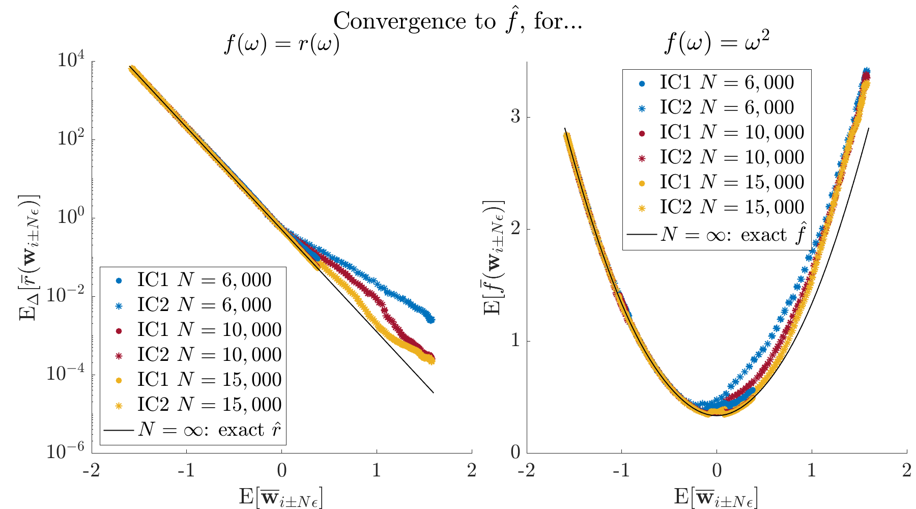
Refer to caption
Figure 15: These plots are the same as in Figure 10, except that we now additionally plot the predicted curve (ω,f^(ω))𝜔^𝑓𝜔(\omega,\hat{f}(\omega)). We see that (𝔼𝐰¯i±Nϵ,𝔼f¯(𝐰i±Nϵ))𝔼subscript¯𝐰plus-or-minus𝑖𝑁italic-ϵ𝔼¯𝑓subscript𝐰plus-or-minus𝑖𝑁italic-ϵ(\mathbb{E}\,\overline{\bf w}_{i\pm N\epsilon},\;\mathbb{E}\,\bar{f}({\bf w}_{i\pm N\epsilon})) converge to the curve as N𝑁N increases. The function f^^𝑓\hat{f} is given by f^(ω)=μK[ω](f)^𝑓𝜔subscriptsuperscript𝜇𝐾delimited-[]𝜔𝑓\hat{f}(\omega)=\mu^{\infty}_{K}[\omega](f), where μK[ω]subscriptsuperscript𝜇𝐾delimited-[]𝜔\mu^{\infty}_{K}[\omega] is defined in (54).
Proposition 6.9.

Define the pmf μK[ω]subscriptsuperscript𝜇𝐾delimited-[]𝜔\mu^{\infty}_{K}[\omega] by

(54) μK[ω](n)=01μK[ω,λ](n)𝑑λ=exp(K2(nω)2)01Q(n,ω,λ)𝑑λ.subscriptsuperscript𝜇𝐾delimited-[]𝜔𝑛superscriptsubscript01subscript𝜇𝐾𝜔𝜆𝑛differential-d𝜆exp𝐾2superscript𝑛𝜔2superscriptsubscript01𝑄𝑛𝜔𝜆differential-d𝜆\mu^{\infty}_{K}[\omega](n)=\int_{0}^{1}\mu_{K}[\omega,\lambda](n)d\lambda=\,\mathrm{exp}\left(-\frac{K}{2}(n-\omega)^{2}\right)\int_{0}^{1}Q(n,\omega,\lambda)d\lambda.

If w(t,x)𝑤𝑡𝑥w(t,x) is irrational, then

(55) |12NϵiN(x±ϵ)μK[ωi,λi](n)μK[𝔼𝐰¯N(x±ϵ)](n)|CN,ϵexp(Kn2/3)12𝑁italic-ϵsubscript𝑖𝑁plus-or-minus𝑥italic-ϵsubscript𝜇𝐾subscript𝜔𝑖subscript𝜆𝑖𝑛subscriptsuperscript𝜇𝐾delimited-[]𝔼subscript¯𝐰𝑁plus-or-minus𝑥italic-ϵ𝑛subscript𝐶𝑁italic-ϵexp𝐾superscript𝑛23\bigg{|}\frac{1}{2N\epsilon}\sum_{i\in{{N(x\pm\epsilon)}}}\mu_{K}[\omega_{i},\lambda_{i}](n)-\mu^{\infty}_{K}\left[\mathbb{E}\,\overline{\bf w}_{{N(x\pm\epsilon)}}\right](n)\bigg{|}\leq C_{N,\epsilon}\,\mathrm{exp}\left(-Kn^{2}/3\right)

for all n𝑛n\in\mathbb{Z}, where CN,ϵ0subscript𝐶𝑁italic-ϵ0C_{N,\epsilon}\to 0 as N,ϵ0formulae-sequence𝑁italic-ϵ0N\to\infty,\,\epsilon\to 0. Letting p(n)exp(Kn2/3)proportional-to𝑝𝑛exp𝐾superscript𝑛23p(n)\propto\,\mathrm{exp}(-Kn^{2}/3) be a pmf on \mathbb{Z}, it follows that (Ef) holds for any fL1(p)𝑓superscript𝐿1𝑝f\in L^{1}(p), with f^(ω)=μK[ω](f)^𝑓𝜔subscriptsuperscript𝜇𝐾delimited-[]𝜔𝑓\hat{f}(\omega)=\mu^{\infty}_{K}[\omega](f).

Let us give an outline for the proof of Proposition 6.9. First, we justify replacing both ωisubscript𝜔𝑖\omega_{i} and 𝔼𝐰¯N(x±ϵ)𝔼subscript¯𝐰𝑁plus-or-minus𝑥italic-ϵ\mathbb{E}\,\bar{\bf w}_{{N(x\pm\epsilon)}} with w:=w(t,x)assign𝑤𝑤𝑡𝑥w:=w(t,x) in (55). This is justified since the ωisubscript𝜔𝑖\omega_{i} converge to w𝑤w by Lemma 6.2, and 𝔼𝐰¯N(x±ϵ)𝔼subscript¯𝐰𝑁plus-or-minus𝑥italic-ϵ\mathbb{E}\,\bar{\bf w}_{{N(x\pm\epsilon)}} converges to w𝑤w by (E). It then remains to show

Lemma 6.10.

Let λisubscript𝜆𝑖\lambda_{i}, iN(x±ϵ)𝑖𝑁plus-or-minus𝑥italic-ϵi\in{N(x\pm\epsilon)} be any numbers such that ωi=λiλi1subscript𝜔𝑖subscript𝜆𝑖subscript𝜆𝑖1\omega_{i}=\lambda_{i}-\lambda_{i-1} satisfy the smoothness Assumption 2 and converge uniformly to w=w(t,x)𝑤𝑤𝑡𝑥w=w(t,x), as in Lemma 6.2. If w𝑤w is irrational, then

(56) |12NϵiN(x±ϵ)μK[w,λi](n)01μK[w,λ](n)𝑑λ|CN,ϵexp(Kn2/3)12𝑁italic-ϵsubscript𝑖𝑁plus-or-minus𝑥italic-ϵsubscript𝜇𝐾𝑤subscript𝜆𝑖𝑛superscriptsubscript01subscript𝜇𝐾𝑤𝜆𝑛differential-d𝜆subscript𝐶𝑁italic-ϵexp𝐾superscript𝑛23\left|\frac{1}{2N\epsilon}\sum_{i\in{N(x\pm\epsilon)}}\mu_{K}[w,\lambda_{i}](n)-\int_{0}^{1}\mu_{K}[w,\lambda](n)d\lambda\right|\leq C_{N,\epsilon}\,\mathrm{exp}\left(-Kn^{2}/3\right)

for all n𝑛n\in\mathbb{Z}, where CN,ϵ0subscript𝐶𝑁italic-ϵ0C_{N,\epsilon}\to 0 as N,ϵ0formulae-sequence𝑁italic-ϵ0N\to\infty,\,\epsilon\to 0.

The rigorous proof of Lemma 6.10 and Proposition 6.9 is given in Appendix C. We briefly sketch the proof of Lemma 6.10 here, to explain the irrationality constraint. To prove the sum in (56) converges to the integral, we show that the points λimod1modulosubscript𝜆𝑖1\lambda_{i}\bmod 1 are asymptotically equidistributed in the unit interval. In other words, we show that the empirical measure PN,ϵsuperscript𝑃𝑁italic-ϵP^{N,\epsilon} given by the average of the point masses at λimod1modulosubscript𝜆𝑖1\lambda_{i}\bmod 1 converges to the Lebesgue measure on the unit interval. To do so, we essentially make the approximation λNx+iλNx+iwsubscript𝜆𝑁𝑥𝑖subscript𝜆𝑁𝑥𝑖𝑤\lambda_{Nx+i}\approx\lambda_{Nx}+iw. Clearly, w𝑤w must be irrational for λimod1modulosubscript𝜆𝑖1\lambda_{i}\bmod 1 to be asymptotically uniformly distributed. Since there is an error incurred by this approximation, we require a quantitative bound on the distance between PN,ϵsuperscript𝑃𝑁italic-ϵP^{N,\epsilon} and Lebesgue measure. For this, we use the Erdős-Turán inequality [2], which says that for a measure ν𝜈\nu on the unit interval, we have

(57) sup(a,b)[0,1]|ν((a,b))(ba)|C(1n+m=1n|ν^(m)|m)subscriptsupremum𝑎𝑏01𝜈𝑎𝑏𝑏𝑎𝐶1𝑛superscriptsubscript𝑚1𝑛^𝜈𝑚𝑚\sup_{(a,b)\subset[0,1]}|\nu((a,b))-(b-a)|\leq C\left(\frac{1}{n}+\sum_{m=1}^{n}\frac{|\hat{\nu}(m)|}{m}\right)

for an absolute constant C𝐶C and any n=1,2,𝑛12n=1,2,\dots, where ν^(m)=exp(2πimx)ν(dx).^𝜈𝑚exp2𝜋𝑖𝑚𝑥𝜈𝑑𝑥\hat{\nu}(m)=\int\,\mathrm{exp}\left(2\pi imx\right)\nu(dx).

Let us consider the limitations due to the constraint w(t,x)𝑤𝑡𝑥w(t,x)\notin\mathbb{Q}. Consider the set of points x𝑥x for which w(t,x)𝑤𝑡𝑥w(t,x) is rational. For this set to have positive Lebesgue measure, there must exist q𝑞q\in\mathbb{Q} such that w(t,x)=q𝑤𝑡𝑥𝑞w(t,x)=q for uncountably many x𝑥x. The case in which these points do not form an interval is pathological and unlikely to appear in practice. Thus, the only kind of non-pathological functions w(t,x)𝑤𝑡𝑥w(t,x) for which this set has positive Lebesgue measure, are the functions for which w(t,x)q𝑤𝑡𝑥𝑞w(t,x)\equiv q\in\mathbb{Q} in some interval. The analysis of this case is beyond the scope of the paper.

6.4 Discussion

We conclude with a few remarks on 𝐰Nsubscript𝐰𝑁\mathbf{w}_{N}’s rough LE.

Why 𝐰Nsubscript𝐰𝑁\mathbf{w}_{N}’s LE is not smooth. The contributing factors are (1) the rough scaling, (2) the discreteness of the microscopic system, and (3) that the distributions Law(zi1,zi)Lawsubscript𝑧𝑖1subscript𝑧𝑖{\mathrm{Law}}(z_{i-1},z_{i}) are Gibbs measures. The contribution of these three factors is evident in the equation

(58) 𝔼wi=uD(λi)uD(λi1)=[λiλi1]+[uo(λimod1)uo(λi1mod1)]=ωi+uo(λimod1)uo(λi1mod1).𝔼subscript𝑤𝑖subscript𝑢𝐷subscript𝜆𝑖subscript𝑢𝐷subscript𝜆𝑖1delimited-[]subscript𝜆𝑖subscript𝜆𝑖1delimited-[]subscript𝑢𝑜modulosubscript𝜆𝑖1subscript𝑢𝑜modulosubscript𝜆𝑖11subscript𝜔𝑖subscript𝑢𝑜modulosubscript𝜆𝑖1subscript𝑢𝑜modulosubscript𝜆𝑖11\begin{split}\mathbb{E}\,w_{i}&=u_{D}(\lambda_{i})-u_{D}(\lambda_{i-1})\\ &=\big{[}\lambda_{i}-\lambda_{i-1}\big{]}+\bigg{[}u_{o}(\lambda_{i}\bmod 1)-u_{o}(\lambda_{i-1}\bmod 1)\bigg{]}\\ &=\omega_{i}+u_{o}(\lambda_{i}\bmod 1)-u_{o}(\lambda_{i-1}\bmod 1).\end{split}

Due to (1) the rough scaling, the λisubscript𝜆𝑖\lambda_{i} are O(N)𝑂𝑁O(N). Due to (2) the discreteness, the expectations 𝔼wi𝔼subscript𝑤𝑖\mathbb{E}\,w_{i} depend on λisubscript𝜆𝑖\lambda_{i} through the nonlinear function uD(λ)=uC(λ)+uo(λ)subscript𝑢𝐷𝜆subscript𝑢𝐶𝜆subscript𝑢𝑜𝜆u_{D}(\lambda)=u_{C}(\lambda)+u_{o}(\lambda) rather than through the linear uC(λ)=λsubscript𝑢𝐶𝜆𝜆u_{C}(\lambda)=\lambda. As a result of the nonlinearity, 𝔼wi𝔼subscript𝑤𝑖\mathbb{E}\,w_{i} depends not only on the smoothly varying finite differences ωi=λiλi1subscript𝜔𝑖subscript𝜆𝑖subscript𝜆𝑖1\omega_{i}=\lambda_{i}-\lambda_{i-1}, but also on the roughly varying λisubscript𝜆𝑖\lambda_{i} themselves. This makes the LE state of 𝐰Nsubscript𝐰𝑁\mathbf{w}_{N} rough. The specific form of the nonlinearity comes from (3) the Gibbs distribution, but this is perhaps less important.

Why Law(𝐰N)subscript𝐰𝑁(\mathbf{w}_{N}) is a rough LE, and an LE at all. The above point explains why the 𝔼wi𝔼subscript𝑤𝑖\mathbb{E}\,w_{i} are roughly varying, implying that the LE state cannot be smooth. But to show Law(𝐰N)Lawsubscript𝐰𝑁{\mathrm{Law}}(\mathbf{w}_{N}) is rough, we needed to show (Ef) is satisfied. We did this using (1) Law(wi)Lawsubscript𝑤𝑖{\mathrm{Law}}(w_{i}) belongs to a two-parameter family with parameters ωisubscript𝜔𝑖\omega_{i}, λisubscript𝜆𝑖\lambda_{i}, (2) the ωisubscript𝜔𝑖\omega_{i} converge uniformly over iN(x±ϵ)𝑖𝑁plus-or-minus𝑥italic-ϵi\in{N(x\pm\epsilon)} to w(t,x)𝑤𝑡𝑥w(t,x) and (3) the empirical distribution defined by the points λimod1modulosubscript𝜆𝑖1\lambda_{i}\bmod 1, iN(x±ϵ)𝑖𝑁plus-or-minus𝑥italic-ϵi\in{N(x\pm\epsilon)} converges to Lebesgue measure. To prove (3), we used that λiλi1=ωisubscript𝜆𝑖subscript𝜆𝑖1subscript𝜔𝑖\lambda_{i}-\lambda_{i-1}=\omega_{i}. However, for (Ef) to hold, any other asymptotically uniformly distributed points λimod1modulosubscript𝜆𝑖1\lambda_{i}\bmod 1 would do. This is an important point because it allows us to think of Law(𝐰N)Lawsubscript𝐰𝑁{\mathrm{Law}}(\mathbf{w}_{N}) not as derived from Law(𝐳N)Lawsubscript𝐳𝑁{\mathrm{Law}}(\mathbf{z}_{N}) (from which the λisubscript𝜆𝑖\lambda_{i} originated), but as a self-standing distribution with certain properties giving rise to a rough LE. This viewpoint can help us identify rough LE states in other contexts.

But does Law(𝐰N)Lawsubscript𝐰𝑁{\mathrm{Law}}(\mathbf{w}_{N}) constitute an LE state at all? Applying Definition 4.1 of an LE state, the joint distribution Law({wi}iN(x±ϵ))Lawsubscriptsubscript𝑤𝑖𝑖𝑁plus-or-minus𝑥italic-ϵ{\mathrm{Law}}(\{w_{i}\}_{i\in{N(x\pm\epsilon)}}) should be asymptotically fully determined, through some parameterization, by w(x)𝑤𝑥w(x) for a continuous function w:[0,1]:𝑤01w:{[0,1]}\to\mathbb{R}. This is not true for our process 𝐰Nsubscript𝐰𝑁\mathbf{w}_{N}, since we need all the numbers λisubscript𝜆𝑖\lambda_{i} to specify the full joint distribution Law({wi}iN(x±ϵ))Lawsubscriptsubscript𝑤𝑖𝑖𝑁plus-or-minus𝑥italic-ϵ{\mathrm{Law}}(\{w_{i}\}_{i\in{N(x\pm\epsilon)}}). However, we have seen that the smoothly varying ωisubscript𝜔𝑖\omega_{i} are the relevant parameters, since the λisubscript𝜆𝑖\lambda_{i} integrate out upon mesoscopic averaging. Since ωiw(t,x)subscript𝜔𝑖𝑤𝑡𝑥\omega_{i}\approx w(t,x) for iN(x±ϵ)𝑖𝑁plus-or-minus𝑥italic-ϵi\in{N(x\pm\epsilon)}, we can still argue that Law({wi}iN(x±ϵ))Lawsubscriptsubscript𝑤𝑖𝑖𝑁plus-or-minus𝑥italic-ϵ{\mathrm{Law}}(\{w_{i}\}_{i\in{N(x\pm\epsilon)}}) is in some sense fully determined by w(t,x)𝑤𝑡𝑥w(t,x).

Impact of Rough LE on the PDE. Recall that the PDE governing the hydrodynamic limit w𝑤w in the rough scaling regime is

(59) tw=xxxxexp(2Kw).subscript𝑡𝑤subscript𝑥𝑥𝑥𝑥exp2𝐾𝑤\partial_{t}w=\partial_{xxxx}\,\mathrm{exp}(-2Kw).

For simplicity, we will take 2K=12𝐾12K=1. We call (59) the “rough w𝑤w PDE”.

We claim that the rough LE state of 𝐰Nsubscript𝐰𝑁\mathbf{w}_{N} causes uDsubscript𝑢𝐷u_{D} to “average out”, and as a result, the argument to the exponential in (59) involves w=λC(w)=uC1(w)𝑤subscript𝜆𝐶𝑤superscriptsubscript𝑢𝐶1𝑤w=\lambda_{C}(w)=u_{C}^{-1}(w) rather than λD(w)=uD1(w)subscript𝜆𝐷𝑤superscriptsubscript𝑢𝐷1𝑤\lambda_{D}(w)=u_{D}^{-1}(w). Our argument will also serve as a correction to the argument given in [17] for the appearance of λCsubscript𝜆𝐶\lambda_{C}.

To make our point, it will be useful to compare a PDE obtained in the rough scaling limit to a corresponding PDE obtained in the smooth-scaling limit. We cannot compare w𝑤w PDEs since the smooth PDE is ill-defined for w=zx𝑤subscript𝑧𝑥w=z_{x}. So instead, let us integrate the rough w𝑤w PDE once with respect to x𝑥x, and then compare the rough z𝑧z PDE to the smooth z𝑧z PDE. We get

(60) tz=xxxexp(λC(zx))subscript𝑡𝑧subscript𝑥𝑥𝑥expsubscript𝜆𝐶subscript𝑧𝑥\partial_{t}z=\partial_{xxx}\,\mathrm{exp}(-\lambda_{C}(z_{x}))

for the rough z𝑧z PDE, where we have written λC(w)subscript𝜆𝐶𝑤\lambda_{C}(w) for w𝑤w (and recall 2K=12𝐾12K=1.) Meanwhile, the smooth z𝑧z PDE can be written in the form

(61) tz=xxxddγexp(γxλD(z))|γ=0.subscript𝑡𝑧evaluated-atsubscript𝑥𝑥𝑥𝑑𝑑𝛾exp𝛾subscript𝑥subscript𝜆𝐷𝑧𝛾0\begin{split}\partial_{t}z=\partial_{xxx}\frac{d}{d\gamma}\,\mathrm{exp}\left(-\gamma\partial_{x}\lambda_{D}(z)\right)\big{|}_{\gamma=0}.\end{split}

The fact that the exponential gets differentiated at zero in (61) has to do with the smooth scaling. For us, the more important difference between the two PDEs is that the smooth z𝑧z PDE contains λDsubscript𝜆𝐷\lambda_{D} while the rough z𝑧z PDE contains λCsubscript𝜆𝐶\lambda_{C}. The function λDsubscript𝜆𝐷\lambda_{D} reflects the discreteness of the microscopic system, so its presence in the PDE (61) governing the non-discrete (i.e. \mathbb{R}-valued) limit z(t,x)𝑧𝑡𝑥z(t,x) is an interesting feature of the smooth scaling regime.

Now, both the smooth and rough z𝑧z PDEs follow from the microscopic dynamics via Nπisubscript𝑁subscript𝜋𝑖\mathcal{L}_{N}\pi_{i}. We have (Nπi)(𝐳)=r(wi+1)3r(wi)+3r(wi1)+r(wi2)subscript𝑁subscript𝜋𝑖𝐳𝑟subscript𝑤𝑖13𝑟subscript𝑤𝑖3𝑟subscript𝑤𝑖1𝑟subscript𝑤𝑖2(\mathcal{L}_{N}\pi_{i})(\mathbf{z})=r(w_{i+1})-3r(w_{i})+3r(w_{i-1})+r(w_{i-2}), where wi=zizi1subscript𝑤𝑖subscript𝑧𝑖subscript𝑧𝑖1w_{i}=z_{i}-z_{i-1}. We then move the three finite differences onto a test function, and replace r(wi)𝑟subscript𝑤𝑖r(w_{i}) with the average of r(wj)𝑟subscript𝑤𝑗r(w_{j}), ji±Nϵ𝑗plus-or-minus𝑖𝑁italic-ϵj\in i\pm N\epsilon. This average should be approximately deterministic, so we replace it with its expectation. E.g. for i=Nx𝑖𝑁𝑥i=\lfloor Nx\rfloor, we consider

(62) 𝔼[12NϵiN(x±ϵ)r(wi)].𝔼delimited-[]12𝑁italic-ϵsubscript𝑖𝑁plus-or-minus𝑥italic-ϵ𝑟subscript𝑤𝑖\mathbb{E}\,\bigg{[}\frac{1}{2N\epsilon}\sum_{i\in{N(x\pm\epsilon)}}r(w_{i})\bigg{]}.

We must then express this average of expectations as a function of the converging microscopic process, and from here the PDE essentially follows. In both the smooth and rough scaling regime, one possible framework for doing so, which centers around Law(𝐳N)Lawsubscript𝐳𝑁{\mathrm{Law}}(\mathbf{z}_{N}), is the following:

  1. 1.

    Introduce parameters λisubscript𝜆𝑖\lambda_{i} such that

    (𝐳N=𝐳)i=1NeKzi2+2Kλizi/𝒵𝝀N.subscript𝐳𝑁𝐳superscriptsubscriptproduct𝑖1𝑁superscript𝑒𝐾superscriptsubscript𝑧𝑖22𝐾subscript𝜆𝑖subscript𝑧𝑖subscript𝒵superscript𝝀𝑁\mathbb{P}(\mathbf{z}_{N}=\mathbf{z})\approx\prod_{i=1}^{N}e^{-Kz_{i}^{2}+2K\lambda_{i}z_{i}}/\mathcal{Z}_{{\bm{\lambda}}^{N}}.

    This is the Gibbs product measure with parameters λisubscript𝜆𝑖\lambda_{i}, i=1,,N𝑖1𝑁i=1,\dots,N.

  2. 2.

    Express (62) in terms of the λisubscript𝜆𝑖\lambda_{i}: using the rate expectation formula (40), we get

    (63) 𝔼[12NϵiN(x±ϵ)r(zizi1)]12NϵiN(x±ϵ)exp(λi1λi).𝔼delimited-[]12𝑁italic-ϵsubscript𝑖𝑁plus-or-minus𝑥italic-ϵ𝑟subscript𝑧𝑖subscript𝑧𝑖112𝑁italic-ϵsubscript𝑖𝑁plus-or-minus𝑥italic-ϵexpsubscript𝜆𝑖1subscript𝜆𝑖\mathbb{E}\,\bigg{[}\frac{1}{2N\epsilon}\sum_{i\in{N(x\pm\epsilon)}}r(z_{i}-z_{i-1})\bigg{]}\approx\frac{1}{2N\epsilon}\sum_{i\in{N(x\pm\epsilon)}}\,\mathrm{exp}(\lambda_{i-1}-\lambda_{i}).
  3. 3.

    Write (63) in terms of the appropriate, converging microscopic process.

We now review the argument in [17] for why λCsubscript𝜆𝐶\lambda_{C} appears in the rough z𝑧z PDE.

Namely, Marzuola and Weare assume λi=λD(𝔼zi)subscript𝜆𝑖subscript𝜆𝐷𝔼subscript𝑧𝑖\lambda_{i}=\lambda_{D}(\mathbb{E}\,z_{i}), and 𝔼ziNz(i/N)𝔼subscript𝑧𝑖𝑁𝑧𝑖𝑁\mathbb{E}\,z_{i}\approx Nz(i/N), where z𝑧z is the hydrodynamic limit of 𝐳Nsubscript𝐳𝑁\mathbf{z}_{N} under amplitude scaling N1superscript𝑁1N^{1} (this corresponds to taking the limit of 𝐡Nsubscript𝐡𝑁\mathbf{h}_{N} in the rough scaling regime). We have omitted the t𝑡t variable in z𝑧z for brevity. They then observe that limκκ1λD(κu)=λC(u)=usubscript𝜅superscript𝜅1subscript𝜆𝐷𝜅𝑢subscript𝜆𝐶𝑢𝑢\lim_{\kappa\to\infty}\kappa^{-1}\lambda_{D}(\kappa u)=\lambda_{C}(u)=u. Using the decomposition λD=id.+λoformulae-sequencesubscript𝜆𝐷idsubscript𝜆𝑜\lambda_{D}=\mathrm{id.}+\lambda_{o} introduced in this paper, this observation is equivalent to saying κ1λD(κu)=u+κ1λo(κu)usuperscript𝜅1subscript𝜆𝐷𝜅𝑢𝑢superscript𝜅1subscript𝜆𝑜𝜅𝑢𝑢\kappa^{-1}\lambda_{D}(\kappa u)=u+\kappa^{-1}\lambda_{o}(\kappa u)\to u as κ𝜅\kappa\to\infty. One then has

(64) λiλD(𝔼zi)λD(Nz(i/N))Nz(i/N),subscript𝜆𝑖subscript𝜆𝐷𝔼subscript𝑧𝑖subscript𝜆𝐷𝑁𝑧𝑖𝑁𝑁𝑧𝑖𝑁\begin{split}\lambda_{i}\approx\lambda_{D}(\mathbb{E}\,z_{i})\approx\lambda_{D}\left(Nz\left(i/N\right)\right)\approx Nz\left(i/N\right),\end{split}

where in the last approximation we have discarded λo(Nz(i/N))subscript𝜆𝑜𝑁𝑧𝑖𝑁\lambda_{o}(Nz(i/N)). Substituting (64) into (63) gives exp(xz(x))expsubscript𝑥𝑧𝑥\,\mathrm{exp}\left(-\partial_{x}z(x)\right) for the average rate expectation. Thus, Marzuola and Weare claim that the reason λCsubscript𝜆𝐶\lambda_{C} arises in the rough PDE is that λD(κu)κλC(u)=κusubscript𝜆𝐷𝜅𝑢𝜅subscript𝜆𝐶𝑢𝜅𝑢\lambda_{D}(\kappa u)\approx\kappa\lambda_{C}(u)=\kappa u for large κ𝜅\kappa, and that in the rough scaling regime, the argument to λDsubscript𝜆𝐷\lambda_{D} is large (in contrast to the smooth scaling regime, where the argument to λDsubscript𝜆𝐷\lambda_{D} is O(1)𝑂1O(1)).

This sequence of approximations is flawed for two reasons, both of which have to do with the fact that we cannot discard order O(1)𝑂1O(1) terms when estimating λisubscript𝜆𝑖\lambda_{i}, since we ultimately need to estimate the finite difference λiλi1subscript𝜆𝑖subscript𝜆𝑖1\lambda_{i}-\lambda_{i-1}. First, as we explained in Section 6.2, the approximation 𝔼zi=Nz(i/N)+o(1)𝔼subscript𝑧𝑖𝑁𝑧𝑖𝑁𝑜1\mathbb{E}\,z_{i}=Nz(i/N)+o(1) would imply that 𝔼wi𝔼subscript𝑤𝑖\mathbb{E}\,w_{i} are smoothly varying and ωi=λiλi1subscript𝜔𝑖subscript𝜆𝑖subscript𝜆𝑖1\omega_{i}=\lambda_{i}-\lambda_{i-1} are roughly varying, when in fact the opposite is true. Therefore, the second approximation in (64) is off by order O(1)𝑂1O(1). The third approximation is also off by O(1)𝑂1O(1), since it discards the non-vanishing λo(Nz(i/N))subscript𝜆𝑜𝑁𝑧𝑖𝑁\lambda_{o}(Nz(i/N)).

A more fundamental reason for why the argument is flawed is that the expression

(65) λiλi1=λD(𝔼zi)λD(𝔼zi1)subscript𝜆𝑖subscript𝜆𝑖1subscript𝜆𝐷𝔼subscript𝑧𝑖subscript𝜆𝐷𝔼subscript𝑧𝑖1\lambda_{i}-\lambda_{i-1}=\lambda_{D}(\mathbb{E}\,z_{i})-\lambda_{D}(\mathbb{E}\,z_{i-1})

is not written in terms of a converging process. Indeed, while we expect N1𝔼ziNz(i/N)superscript𝑁superscript𝑁1𝔼subscript𝑧𝑖𝑧𝑖𝑁N^{-1}\mathbb{E}\,z_{i}\stackrel{{\scriptstyle N}}{{\approx}}z(i/N), the expression (65) depends on the non-converging 𝔼zimod1modulo𝔼subscript𝑧𝑖1\mathbb{E}\,z_{i}\bmod 1. But the third step above requires us to write the average of exp(λi1λi)expsubscript𝜆𝑖1subscript𝜆𝑖\,\mathrm{exp}(\lambda_{i-1}-\lambda_{i}) in terms of a converging process, and it is not at all clear how to do this using (65). This is where the 𝐰Nsubscript𝐰𝑁\mathbf{w}_{N} rough LE comes in. But before we continue, note that in the smooth scaling regime (65) is written in terms of a converging process: from numerical simulations (see Figure 4), we should have 𝔼ziNz(i/N)superscript𝑁𝔼subscript𝑧𝑖𝑧𝑖𝑁\mathbb{E}\,z_{i}\stackrel{{\scriptstyle N}}{{\approx}}z(i/N) and N(𝔼zi𝔼zi1)Nzx(i/N).superscript𝑁𝑁𝔼subscript𝑧𝑖𝔼subscript𝑧𝑖1subscript𝑧𝑥𝑖𝑁N(\mathbb{E}\,z_{i}-\mathbb{E}\,z_{i-1})\stackrel{{\scriptstyle N}}{{\approx}}z_{x}(i/N). Using an extra power of N𝑁N multiplying the rate expectation average (63), we get the smooth z𝑧z PDE (61), which involves λDsubscript𝜆𝐷\lambda_{D}.

Returning to the rough scaling regime, another framework for deriving the PDE parallels 1-3 above, but instead uses the parameterization Law(wi)μK[ωi,λi]Lawsubscript𝑤𝑖subscript𝜇𝐾subscript𝜔𝑖subscript𝜆𝑖{\mathrm{Law}}(w_{i})\approx\mu_{K}[\omega_{i},\lambda_{i}]. Since we know the ωisubscript𝜔𝑖\omega_{i} are smoothly varying, uniformly over iN(x±ϵ)𝑖𝑁plus-or-minus𝑥italic-ϵi\in{N(x\pm\epsilon)}, let us for simplicity assume ωiωsubscript𝜔𝑖𝜔\omega_{i}\equiv\omega for iN(x±ϵ)𝑖𝑁plus-or-minus𝑥italic-ϵi\in{N(x\pm\epsilon)}. We then have

(66) 𝔼[12NϵiN(x±ϵ)r(wi)]exp(ω).𝔼delimited-[]12𝑁italic-ϵsubscript𝑖𝑁plus-or-minus𝑥italic-ϵ𝑟subscript𝑤𝑖exp𝜔\mathbb{E}\,\bigg{[}\frac{1}{2N\epsilon}\sum_{i\in{N(x\pm\epsilon)}}r(w_{i})\bigg{]}\approx\,\mathrm{exp}(-\omega).

It remains to write ω𝜔\omega in terms of a converging process. Of course, we already know from Lemma 6.2 that ω𝔼𝐰¯N(x±ϵ)𝜔𝔼subscript¯𝐰𝑁plus-or-minus𝑥italic-ϵ\omega\approx\mathbb{E}\,\overline{\bf w}_{{N(x\pm\epsilon)}}, which is our desired process converging to w=zx𝑤subscript𝑧𝑥w=z_{x} (we think of z𝑧z as the antiderivative of w𝑤w). But we got to that lemma by assuming the Gibbs distribution on 𝐳Nsubscript𝐳𝑁\mathbf{z}_{N}. Using only the perspective of the 𝐰Nsubscript𝐰𝑁\mathbf{w}_{N} distribution, and the insight that the λimod1modulosubscript𝜆𝑖1\lambda_{i}\bmod 1 are asymptotically uniformly distributed, we have

12NϵiN(x±ϵ)Law(wi)12NϵiN(x±ϵ)μK[ω,λi]μK[ω].12𝑁italic-ϵsubscript𝑖𝑁plus-or-minus𝑥italic-ϵLawsubscript𝑤𝑖12𝑁italic-ϵsubscript𝑖𝑁plus-or-minus𝑥italic-ϵsubscript𝜇𝐾𝜔subscript𝜆𝑖subscriptsuperscript𝜇𝐾delimited-[]𝜔\frac{1}{2N\epsilon}\sum_{i\in{{N(x\pm\epsilon)}}}{\mathrm{Law}}(w_{i})\approx\frac{1}{2N\epsilon}\sum_{i\in{{N(x\pm\epsilon)}}}\mu_{K}[\omega,\lambda_{i}]\approx\mu^{\infty}_{K}[\omega].

Thus, we should think of ω𝜔\omega as the unique parameter such that

𝔼𝐰¯N(x±ϵ)=m1(iN(x±ϵ)Law(wi)/2Nϵ)=m1(μK[ω]).𝔼subscript¯𝐰𝑁plus-or-minus𝑥italic-ϵsubscript𝑚1subscript𝑖𝑁plus-or-minus𝑥italic-ϵLawsubscript𝑤𝑖2𝑁italic-ϵsubscript𝑚1subscriptsuperscript𝜇𝐾delimited-[]𝜔\mathbb{E}\,\overline{\bf w}_{{N(x\pm\epsilon)}}=m_{1}\bigg{(}\!\sum_{i\in{{N(x\pm\epsilon)}}}{\mathrm{Law}}(w_{i})/2N\epsilon\bigg{)}=m_{1}(\mu^{\infty}_{K}[\omega]).

Now, recall our computation (53) of m1(μK[ω])subscript𝑚1subscriptsuperscript𝜇𝐾delimited-[]𝜔m_{1}(\mu^{\infty}_{K}[\omega]), which finally explains our claim about uDsubscript𝑢𝐷u_{D} averaging out:

(67) m1(μK[ω])=01uD(λ)01uD(λω)=uC(ω)=ω.subscript𝑚1subscriptsuperscript𝜇𝐾delimited-[]𝜔superscriptsubscript01subscript𝑢𝐷𝜆superscriptsubscript01subscript𝑢𝐷𝜆𝜔subscript𝑢𝐶𝜔𝜔m_{1}(\mu^{\infty}_{K}[\omega])=\int_{0}^{1}u_{D}(\lambda)-\int_{0}^{1}u_{D}(\lambda-\omega)=u_{C}(\omega)=\omega.

Therefore, ω=uc1(𝔼𝐰¯N(x±ϵ))=λC(𝔼𝐰¯N(x±ϵ))𝜔superscriptsubscript𝑢𝑐1𝔼subscript¯𝐰𝑁plus-or-minus𝑥italic-ϵsubscript𝜆𝐶𝔼subscript¯𝐰𝑁plus-or-minus𝑥italic-ϵ\omega=u_{c}^{-1}(\mathbb{E}\,\overline{\bf w}_{{N(x\pm\epsilon)}})=\lambda_{C}(\mathbb{E}\,\overline{\bf w}_{{N(x\pm\epsilon)}}).

To summarize, we end up integrating uDsubscript𝑢𝐷u_{D} over λ[0,1]𝜆01\lambda\in[0,1] because the λimod1modulosubscript𝜆𝑖1\lambda_{i}\bmod 1 are asymptotically uniformly distributed (and roughly varying). Therefore the rough LE state of 𝐰Nsubscript𝐰𝑁\mathbf{w}_{N} led to the integration (67) which erased the discreteness in uDsubscript𝑢𝐷u_{D}, so we ended up not with λD=uD1subscript𝜆𝐷superscriptsubscript𝑢𝐷1\lambda_{D}=u_{D}^{-1} but with λCsubscript𝜆𝐶\lambda_{C}. Interestingly enough, 𝐰Nsubscript𝐰𝑁\mathbf{w}_{N} owes its rough LE state to the discreteness of the microscopic system. And this rough LE state, in turn, caused the discreteness to be washed out in the continuum limit!

7 Conclusion

In this paper, we have discovered a new, rough local equilibrium (LE) state, and studied its properties through the lens of the three key limits (V), (E), and (Ef). These limits do hold under a rough LE, but the stronger pointwise limits (E\,{}^{\prime}), (Ef\,{}^{\prime}) do not. This is because mesoscopic window averaging is essential to smooth out the roughness of ensemble averages. Indeed, unlike in smooth LE states, most observable expectations 𝔼[f(wi)]𝔼delimited-[]𝑓subscript𝑤𝑖\mathbb{E}\,[f(w_{i})] vary roughly with i𝑖i (that f(wi)𝑓subscript𝑤𝑖f(w_{i}) vary roughly before taking expectations is unsurprising). In Section 6, we uncovered the mechanism underlying the convergence (Ef): mesoscopic averages of the single site marginals Law(wi)Lawsubscript𝑤𝑖{\mathrm{Law}}(w_{i}) belong to a mean-parameterized measure family in the N𝑁N\to\infty, ϵ0italic-ϵ0\epsilon\to 0 limit. Finally, we explained in Section 6.4 why 𝐰Nsubscript𝐰𝑁\mathbf{w}_{N}’s rough LE state is a product of the rough scaling regime and discreteness. In turn, the rough LE led to an integration which erased the discreteness of uDsubscript𝑢𝐷u_{D}, leaving λCsubscript𝜆𝐶\lambda_{C} rather than λD=uD1subscript𝜆𝐷superscriptsubscript𝑢𝐷1\lambda_{D}=u_{D}^{-1} in the PDE.

The rough LE state we have discovered is not isolated to the 𝐰Nsubscript𝐰𝑁\mathbf{w}_{N} process studied here. In [11], we show that a crystal surface process with Metropolis-type jump rates also has a rough LE state. Specifically, we study 𝐯Nsubscript𝐯𝑁\mathbf{v}_{N} given by a third order finite difference of 𝐡Nsubscript𝐡𝑁\mathbf{h}_{N}, which is scaled as O(N3)𝑂superscript𝑁3O(N^{3}). For the Metropolis rate process, this is the scaling regime leading to a nontrivial PDE with exponential nonlinearity. (See [5] for an informal derivation of the rough scaling PDE limit of the Metropolis height process). Even though Law(𝐳N)Lawsubscript𝐳𝑁{\mathrm{Law}}(\mathbf{z}_{N}) is not local Gibbs, the LE state of 𝐯Nsubscript𝐯𝑁\mathbf{v}_{N} is still rough. This reinforces the centrality of (1) the rough scaling and (2) the discreteness of the microscopic system in contributing to the rough LE state. Interestingly, the LE state of 𝐯Nsubscript𝐯𝑁\mathbf{v}_{N} is qualitatively very similar to the LE state of 𝐰Nsubscript𝐰𝑁\mathbf{w}_{N} for the Arrhenius process. This similarity could be related to the fact that the invariant measure for the 𝐳Nsubscript𝐳𝑁\mathbf{z}_{N} processes are the same: the λi0subscript𝜆𝑖0\lambda_{i}\equiv 0 standard Gibbs measure Φ(z)exp(KH(z))proportional-toΦ𝑧exp𝐾𝐻𝑧\Phi(z)\propto\,\mathrm{exp}\left(-KH(z)\right). However, this merits further investigation, which we leave for future work.

Appendix A Local Equilibrium of Zero Range Process

This section summarizes results from Chapter 2.3 in [12]. We stated in the main text that the local equilibrium measure of the zero range process is given by a product of mean-parameterized measures μ[]𝜇delimited-[]\mu[\cdot], of the form Law(𝐯N)i=1Nμ[v(t,i/N)].{\mathrm{Law}}(\mathbf{v}_{N})\approx\otimes_{i=1}^{N}\mu\left[v\left(t,i/N\right)\right]. This is true, but it is slightly more convenient to parameterize these measures using another parameter which is not the mean. To that end, define a family {ν[ϕ]0ϕ<}conditional-set𝜈delimited-[]italic-ϕ0italic-ϕ\{\nu[\phi]\mid 0\leq\phi<\infty\} of measure on {0,1,2,}012\{0,1,2,\dots\}, via

ν[ϕ](n)=1Z(ϕ)ϕng(n)!,whereg(n)!=k=1ng(k),formulae-sequence𝜈delimited-[]italic-ϕ𝑛1𝑍italic-ϕsuperscriptitalic-ϕ𝑛𝑔𝑛where𝑔𝑛superscriptsubscriptproduct𝑘1𝑛𝑔𝑘\nu[\phi](n)=\frac{1}{Z(\phi)}\frac{\phi^{n}}{g(n)!},\quad\text{where}\quad g(n)!=\prod_{k=1}^{n}g(k),

and g(0)!=1𝑔01g(0)!=1 by convention. Here, Z(ϕ)𝑍italic-ϕZ(\phi) is the normalization constant Z(ϕ)=n=0ϕn/g(n)!𝑍italic-ϕsuperscriptsubscript𝑛0superscriptitalic-ϕ𝑛𝑔𝑛Z(\phi)=\sum_{n=0}^{\infty}\phi^{n}/g(n)!. We assume that the rates g(n)𝑔𝑛g(n) are such that Z(ϕ)<𝑍italic-ϕZ(\phi)<\infty for all ϕ0italic-ϕ0\phi\geq 0, and that limϕZ(ϕ)=subscriptitalic-ϕ𝑍italic-ϕ\lim_{\phi\to\infty}Z(\phi)=\infty. Define

v(ϕ)=m1(ν[ϕ])=n=0n1Z(ϕ)ϕng(n)!.𝑣italic-ϕsubscript𝑚1𝜈delimited-[]italic-ϕsuperscriptsubscript𝑛0𝑛1𝑍italic-ϕsuperscriptitalic-ϕ𝑛𝑔𝑛v(\phi)=m_{1}(\nu[\phi])=\sum_{n=0}^{\infty}n\frac{1}{Z(\phi)}\frac{\phi^{n}}{g(n)!}.

The assumptions on Z(ϕ)𝑍italic-ϕZ(\phi) guarantee that v(ϕ)𝑣italic-ϕv(\phi) is strictly increasing and that v:++:𝑣subscriptsubscriptv:\mathbb{R}_{+}\to\mathbb{R}_{+} is bijective. Therefore, our desired mean-parameterized LE measure family is {μ[v]v0}conditional-set𝜇delimited-[]𝑣𝑣0\{\mu[v]\mid v\geq 0\}, where μ[v]=ν[ϕ(v)]𝜇delimited-[]𝑣𝜈delimited-[]italic-ϕ𝑣\mu[v]=\nu[\phi(v)] and ϕ=v1italic-ϕsuperscript𝑣1\phi=v^{-1}.

Recall that given a mean-parameterized measure family μ[]𝜇delimited-[]\mu[\cdot] and an observable f𝑓f, we define f^(v)=μ[v](f)^𝑓𝑣𝜇delimited-[]𝑣𝑓\hat{f}(v)=\mu[v](f). Therefore, for the zero range LE, we compute f^^𝑓\hat{f} to be

(68) f^(v)=n=0f(n)1Z(ϕ(v))ϕ(v)ng(n)!.^𝑓𝑣superscriptsubscript𝑛0𝑓𝑛1𝑍italic-ϕ𝑣italic-ϕsuperscript𝑣𝑛𝑔𝑛\hat{f}(v)=\sum_{n=0}^{\infty}f(n)\frac{1}{Z(\phi(v))}\frac{\phi(v)^{n}}{g(n)!}.

We use Equation (68) to compute the (v,f^(v))𝑣^𝑓𝑣(v,\hat{f}(v)) curves shown in Figure 3.

Appendix B Numerics

B.1 Kinetic Monte Carlo

Each of the interacting particle systems discussed in this paper is a Markov jump process {𝐯~N(t)}t0subscriptsubscript~𝐯𝑁𝑡𝑡0\{\tilde{\mathbf{v}}_{N}(t)\}_{t\geq 0}, the paths of which are step functions, with 𝐯~N(t)=𝐯Nksubscript~𝐯𝑁𝑡superscriptsubscript𝐯𝑁𝑘\tilde{\mathbf{v}}_{N}(t)=\mathbf{v}_{N}^{k} when t[tk,tk+1)𝑡subscript𝑡𝑘subscript𝑡𝑘1t\in[t_{k},t_{k+1}). Therefore, simulating the process in a time interval [0,T(N)]0𝑇𝑁[0,T(N)] amounts to drawing pairs (𝐯~Nk,tk)superscriptsubscript~𝐯𝑁𝑘subscript𝑡𝑘(\tilde{\mathbf{v}}_{N}^{k},t_{k}) according to the law of the process until tksubscript𝑡𝑘t_{k} first exceeds T(N)𝑇𝑁T(N). We do so using the Kinetic Monte Carlo algorithm (KMC) [8].

To simulate processes 𝐯N(t)=𝐯~N(Nαt)subscript𝐯𝑁𝑡subscript~𝐯𝑁superscript𝑁𝛼𝑡\mathbf{v}_{N}(t)=\tilde{\mathbf{v}}_{N}(N^{\alpha}t), N=1,2,𝑁12N=1,2,\dots we do the following. First, we fix a macroscopic initial profile v0:[0,1]:subscript𝑣001v_{0}:{[0,1]}\to\mathbb{R} and a macroscopic time t𝑡t. Next, we construct a sequence of distributions μ0Nsubscriptsuperscript𝜇𝑁0\mu^{N}_{0}, N=1,2,𝑁12N=1,2,\dots associated to v0subscript𝑣0v_{0} as in Definition 2.1. For simplicity, we take μ0Nsubscriptsuperscript𝜇𝑁0\mu^{N}_{0} such that 𝔼μ0N[vi(0)]=v(i/N)subscript𝔼subscriptsuperscript𝜇𝑁0delimited-[]subscript𝑣𝑖0𝑣𝑖𝑁\mathbb{E}\,_{\mu^{N}_{0}}[v_{i}(0)]=v(i/N). For a given N𝑁N, we draw n𝑛n initial profiles 𝐯N(k)(0)superscriptsubscript𝐯𝑁𝑘0\mathbf{v}_{N}^{(k)}(0), k=1,,n𝑘1𝑛k=1,\dots,n independently from μ0Nsubscriptsuperscript𝜇𝑁0\mu^{N}_{0}. We then use KMC to generate independent processes 𝐯N(k)superscriptsubscript𝐯𝑁𝑘\mathbf{v}_{N}^{(k)} corresponding to the initial profiles, evolving each of them forward until time Nαtsuperscript𝑁𝛼𝑡N^{\alpha}t. To estimate expectations 𝔼[f(𝐯N(t))]𝔼delimited-[]𝑓subscript𝐯𝑁𝑡\mathbb{E}\,[f(\mathbf{v}_{N}(t))], we then take

(69) 𝔼[f(𝐯N(t))]𝔼n[f(𝐯N(t))]:=1nk=1nf(𝐯~N(k)(Nαt)).𝔼delimited-[]𝑓subscript𝐯𝑁𝑡superscript𝔼𝑛delimited-[]𝑓subscript𝐯𝑁𝑡assign1𝑛superscriptsubscript𝑘1𝑛𝑓superscriptsubscript~𝐯𝑁𝑘superscript𝑁𝛼𝑡\mathbb{E}\,[f(\mathbf{v}_{N}(t))]\approx\mathbb{E}\,^{n}[f(\mathbf{v}_{N}(t))]:=\frac{1}{n}\sum_{k=1}^{n}f(\tilde{\mathbf{v}}_{N}^{(k)}(N^{\alpha}t)).

For the crystal processes simulated in this paper — the slope process 𝐳Nsubscript𝐳𝑁\mathbf{z}_{N} in the smooth scaling regime, and the curvature process 𝐰Nsubscript𝐰𝑁\mathbf{w}_{N} in the rough scaling regime — it is simpler to evolve forward the associated height process. We therefore first fix an initial height profile h0subscript0h_{0}, and draw hi(0)=Nβh0(i/N)+ξisubscript𝑖0superscript𝑁𝛽subscript0𝑖𝑁subscript𝜉𝑖h_{i}(0)=\lfloor N^{\beta}h_{0}(i/N)\rfloor+\xi_{i}, where β=1,2𝛽12\beta=1,2 for the smooth and rough scaling regimes, respectively, and ξisubscript𝜉𝑖\xi_{i} are independent Bernoullis. One can check that the induced distribution μ0Nsubscriptsuperscript𝜇𝑁0\mu^{N}_{0} of initial slope or curvature profiles is associated to h0superscriptsubscript0h_{0}^{\prime} or h0′′superscriptsubscript0′′h_{0}^{\prime\prime} as in Definition 2.1, with β=0𝛽0\beta=0. We then evolve 𝐡N(t)subscript𝐡𝑁𝑡\mathbf{h}_{N}(t) forward, and recover the process of interest by taking one or two finite differences.

B.2 Time Averaging

The remainder of Appendix B pertains to numerical computations for the rough scaling curvature process 𝐰N(t)=𝐰~N(N4t)subscript𝐰𝑁𝑡subscript~𝐰𝑁superscript𝑁4𝑡\mathbf{w}_{N}(t)=\tilde{\mathbf{w}}_{N}(N^{4}t). As discussed in the main text, the spatially averaged rate observable f(𝐰N)=r¯(𝐰i±Nϵ)𝑓subscript𝐰𝑁¯𝑟subscript𝐰plus-or-minus𝑖𝑁italic-ϵf(\mathbf{w}_{N})=\bar{r}({\bf w}_{i\pm N\epsilon}) needed to check (Ef) has a very large variance. To get much lower variance, and low bias, estimates of this expectation, we will show that for ΔΔ\Delta chosen appropriately, we have

(70) 𝔼[f(𝐰N(t))]𝔼Δ[f(𝐰N(t))]:=1ΔIt𝔼[f(𝐰N(s))]𝑑s,𝔼delimited-[]𝑓subscript𝐰𝑁𝑡subscript𝔼Δdelimited-[]𝑓subscript𝐰𝑁𝑡assign1Δsubscriptsubscript𝐼𝑡𝔼delimited-[]𝑓subscript𝐰𝑁𝑠differential-d𝑠\mathbb{E}\,[f(\mathbf{w}_{N}(t))]\approx\mathbb{E}\,_{\Delta}[f(\mathbf{w}_{N}(t))]:=\frac{1}{\Delta}\int_{I_{t}}\mathbb{E}\,[f(\mathbf{w}_{N}(s))]ds,

where Itsubscript𝐼𝑡I_{t} is any length ΔΔ\Delta interval containing t𝑡t. We estimate the time averaged expectation using the significantly lower variance estimator below:

(71) 𝔼Δ[f(𝐰N(t))]𝔼Δn[f(𝐰N(t))]:=1nk=1n1N4ΔN4Itf(𝐰~N(k)(s))𝑑s.subscript𝔼Δdelimited-[]𝑓subscript𝐰𝑁𝑡subscriptsuperscript𝔼𝑛Δdelimited-[]𝑓subscript𝐰𝑁𝑡assign1𝑛superscriptsubscript𝑘1𝑛1superscript𝑁4Δsubscriptsuperscript𝑁4subscript𝐼𝑡𝑓superscriptsubscript~𝐰𝑁𝑘𝑠differential-d𝑠\mathbb{E}\,_{\Delta}[f(\mathbf{w}_{N}(t))]\approx\mathbb{E}\,^{n}_{\Delta}[f(\mathbf{w}_{N}(t))]:=\frac{1}{n}\sum_{k=1}^{n}\frac{1}{N^{4}\Delta}\int_{N^{4}I_{t}}f(\tilde{\mathbf{w}}_{N}^{(k)}(s))ds.

The time integrals for each path 𝐰N(k)superscriptsubscript𝐰𝑁𝑘\mathbf{w}_{N}^{(k)} can be computed exactly because 𝐰N(t)subscript𝐰𝑁𝑡\mathbf{w}_{N}(t) is a step function in time. We will show that there is a ΔΔ\Delta such that (70) holds for each rate function f(𝐰N)=r(wi)𝑓subscript𝐰𝑁𝑟subscript𝑤𝑖f(\mathbf{w}_{N})=r(w_{i}), i=1,,N𝑖1𝑁i=1,\dots,N. This same ΔΔ\Delta will work to estimate 𝔼r¯(𝐰N(x±ϵ))𝔼¯𝑟subscript𝐰𝑁plus-or-minus𝑥italic-ϵ\mathbb{E}\,\bar{r}({\bf w}_{{N(x\pm\epsilon)}}). First, we choose ΔΔ\Delta small enough that decreasing ΔΔ\Delta further has no effect on the estimator 𝔼Δn[r(wi)]subscriptsuperscript𝔼𝑛Δdelimited-[]𝑟subscript𝑤𝑖\mathbb{E}\,^{n}_{\Delta}[r(w_{i})], except perhaps to increase its variance. This is shown in the left panel of Figure 16, with N=6000𝑁6000N=6000. We take Δ=1014Δsuperscript1014\Delta=10^{-14}, and note that the estimators 𝔼Δn[r(wi)]subscriptsuperscript𝔼𝑛Δdelimited-[]𝑟subscript𝑤𝑖\mathbb{E}\,^{n}_{\Delta}[r(w_{i})], 𝔼Δ/2n[r(wi)]subscriptsuperscript𝔼𝑛Δ2delimited-[]𝑟subscript𝑤𝑖\mathbb{E}\,^{n}_{\Delta/2}[r(w_{i})], and 𝔼Δ/4n[r(wi)]subscriptsuperscript𝔼𝑛Δ4delimited-[]𝑟subscript𝑤𝑖\mathbb{E}\,^{n}_{\Delta/4}[r(w_{i})] are all extremely close to one another (with n=1000𝑛1000n=1000). Next, we compare 𝔼n[r(wi)]superscript𝔼𝑛delimited-[]𝑟subscript𝑤𝑖\mathbb{E}\,^{n}[r(w_{i})] to 𝔼Δ[r(wi)]subscript𝔼Δdelimited-[]𝑟subscript𝑤𝑖\mathbb{E}\,_{\Delta}[r(w_{i})] for increasing n𝑛n. This is shown in the right panel of Figure 16. It is clear that with increasing n𝑛n, the instantaneous-time rate expectation estimator 𝔼n[r(wi)]superscript𝔼𝑛delimited-[]𝑟subscript𝑤𝑖\mathbb{E}\,^{n}[r(w_{i})] approaches 𝔼Δ[r(wi)]subscript𝔼Δdelimited-[]𝑟subscript𝑤𝑖\mathbb{E}\,_{\Delta}[r(w_{i})], although even for the largest n=106𝑛superscript106n=10^{6}, 𝔼n[r(wi)]superscript𝔼𝑛delimited-[]𝑟subscript𝑤𝑖\mathbb{E}\,^{n}[r(w_{i})] has not yet converged. Increasing n𝑛n further is computationally intractable.
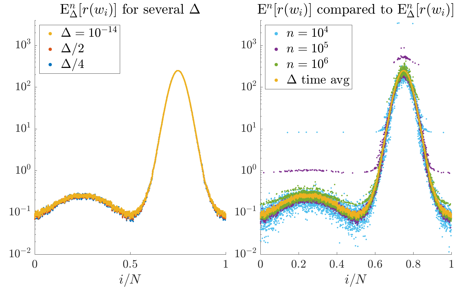
Refer to caption
Figure 16: Left: for a very small ΔΔ\Delta, we show that the effect of decreasing ΔΔ\Delta on the estimator 𝔼Δn[r(wi)]subscriptsuperscript𝔼𝑛Δdelimited-[]𝑟subscript𝑤𝑖\mathbb{E}\,^{n}_{\Delta}[r(w_{i})] is negligible. Right: As n𝑛n increases, the instantaneous-time rate expectation estimator 𝔼n[r(wi)]superscript𝔼𝑛delimited-[]𝑟subscript𝑤𝑖\mathbb{E}\,^{n}[r(w_{i})] approaches 𝔼Δ[r(wi)]subscript𝔼Δdelimited-[]𝑟subscript𝑤𝑖\mathbb{E}\,_{\Delta}[r(w_{i})].

B.3 Choice of ϵ(N)italic-ϵ𝑁\epsilon(N) to verify (E)

Recall (E): 12NϵiN(x±ϵ)𝔼wi(t)w(t,x)12𝑁italic-ϵsubscript𝑖𝑁plus-or-minus𝑥italic-ϵ𝔼subscript𝑤𝑖𝑡𝑤𝑡𝑥\frac{1}{2N\epsilon}\sum_{{i\in{N(x\pm\epsilon)}}}\mathbb{E}\,w_{i}(t)\to w(t,x) as N,ϵ0formulae-sequence𝑁italic-ϵ0N\to\infty,\,\epsilon\to 0.

Refer to caption
Figure 17: 𝔼[𝐰¯i±Nϵ]𝔼delimited-[]subscript¯𝐰plus-or-minus𝑖𝑁italic-ϵ\mathbb{E}\,[\overline{\bf w}_{i\pm N\epsilon}] for fixed N𝑁N and decreasing ϵitalic-ϵ\epsilon, on three scales. From the perspective of the large and medium scales, 𝔼[𝐰¯i±Nϵ]𝔼delimited-[]subscript¯𝐰plus-or-minus𝑖𝑁italic-ϵ\mathbb{E}\,[\overline{\bf w}_{i\pm N\epsilon}] has nearly converged for ϵ0.011italic-ϵ0.011\epsilon\leq 0.011.

We use the following proxy for N,ϵ0formulae-sequence𝑁italic-ϵ0N\to\infty,\epsilon\to 0 convergence. For each N𝑁N, we choose a “good” ϵ(N)italic-ϵ𝑁\epsilon(N): for ϵ>ϵ(N)italic-ϵitalic-ϵ𝑁\epsilon>\epsilon(N), 𝔼[𝐰¯i±Nϵ]𝔼delimited-[]subscript¯𝐰plus-or-minus𝑖𝑁italic-ϵ\mathbb{E}\,[\overline{\bf w}_{i\pm N\epsilon}] is smooth but biased, and for ϵ<ϵ(N)italic-ϵitalic-ϵ𝑁\epsilon<\epsilon(N), it is unbiased but rough. We then check that 𝔼[𝐰¯N(x±ϵ(N))]𝔼delimited-[]subscript¯𝐰𝑁plus-or-minus𝑥italic-ϵ𝑁\mathbb{E}\,[\overline{\bf w}_{N(x\pm\epsilon(N))}] is converging as N𝑁N\to\infty. Figure 17 shows 𝔼[𝐰¯i±Nϵ]𝔼delimited-[]subscript¯𝐰plus-or-minus𝑖𝑁italic-ϵ\mathbb{E}\,[\overline{\bf w}_{i\pm N\epsilon}] for N=15000𝑁15000N=15000 and several values of ϵitalic-ϵ\epsilon, on three scales. The largest scale is shown in the lefthand plot, with the medium scale region indicated by the rectangle on the bottom right. The medium and small scales are shown in the righthand plot. Relative to the variation in the range on the large and medium scales, 𝔼[𝐰¯i±Nϵ]𝔼delimited-[]subscript¯𝐰plus-or-minus𝑖𝑁italic-ϵ\mathbb{E}\,[\overline{\bf w}_{i\pm N\epsilon}] has nearly converged for ϵ0.011italic-ϵ0.011\epsilon\leq 0.011. But it has not converged on the small scale, which we use to pick ϵ(N)italic-ϵ𝑁\epsilon(N). For N=15000𝑁15000N=15000 shown here, we take ϵ(N)=0.008italic-ϵ𝑁0.008\epsilon(N)=0.008. The process is similar for other N𝑁N’s.

B.4 Local Gibbs Computations

Refer to caption
Figure 18: ω^i(1)superscriptsubscript^𝜔𝑖1\hat{\omega}_{i}^{(1)}, ω^i(2)superscriptsubscript^𝜔𝑖2\hat{\omega}_{i}^{(2)} are the estimators used to verify Props 1.1, 1.2. They become closer for larger N𝑁N.

We use two different estimates of ωisubscript𝜔𝑖\omega_{i} in the relative entropy calculation H(Law(wi)|μK[ωi,λi])𝐻conditionalLawsubscript𝑤𝑖subscript𝜇𝐾subscript𝜔𝑖subscript𝜆𝑖H(\mathrm{Law}(w_{i})\,|\,\mu_{K}[\omega_{i},\lambda_{i}]) needed to check Property 1.1, and for the finite difference computation N|ωi+1ωi|𝑁subscript𝜔𝑖1subscript𝜔𝑖N|\omega_{i+1}-\omega_{i}| in Property 1.2. We call these estimates ω^i(1)superscriptsubscript^𝜔𝑖1\hat{\omega}_{i}^{(1)} and ω^i(2)superscriptsubscript^𝜔𝑖2\hat{\omega}_{i}^{(2)}, respectively.

For the relative entropy computation, we find λisubscript𝜆𝑖\lambda_{i} as λi=λD(𝔼Δ[zi])subscript𝜆𝑖subscript𝜆𝐷subscript𝔼Δdelimited-[]subscript𝑧𝑖\lambda_{i}=\lambda_{D}(\mathbb{E}\,_{\Delta}[z_{i}]), where 𝔼Δ[zi]subscript𝔼Δdelimited-[]subscript𝑧𝑖\mathbb{E}\,_{\Delta}[z_{i}] is computed by taking cumulative sums of the 𝔼Δ[wj]subscript𝔼Δdelimited-[]subscript𝑤𝑗\mathbb{E}\,_{\Delta}[w_{j}] and then subtracting off a constant to ensure i𝔼Δ[zi]=0subscript𝑖subscript𝔼Δdelimited-[]subscript𝑧𝑖0\sum_{i}\mathbb{E}\,_{\Delta}[z_{i}]=0. Then

(72) ω^i(1)=λD(𝔼Δ[zi])λD(𝔼Δ[zi1]).superscriptsubscript^𝜔𝑖1subscript𝜆𝐷subscript𝔼Δdelimited-[]subscript𝑧𝑖subscript𝜆𝐷subscript𝔼Δdelimited-[]subscript𝑧𝑖1\hat{\omega}_{i}^{(1)}=\lambda_{D}(\mathbb{E}\,_{\Delta}[z_{i}])-\lambda_{D}(\mathbb{E}\,_{\Delta}[z_{i-1}]).

This determines the measure μK[ω^i(1),λi]subscript𝜇𝐾superscriptsubscript^𝜔𝑖1subscript𝜆𝑖\mu_{K}[\hat{\omega}_{i}^{(1)},\lambda_{i}] to which we compare Law(wi(t))Lawsubscript𝑤𝑖𝑡{\mathrm{Law}}(w_{i}(t)). To estimate the distributions Law(wi(t))Lawsubscript𝑤𝑖𝑡{\mathrm{Law}}(w_{i}(t)), we compute empirical probability mass functions based on 100010001000 independent samples of wi(t)subscript𝑤𝑖𝑡w_{i}(t).

To test the smoothness of ωisubscript𝜔𝑖\omega_{i}, we compute ωisubscript𝜔𝑖\omega_{i} as

(73) ω^i(2)=log(𝔼Δ[r(wi)])/(2K).superscriptsubscript^𝜔𝑖2subscript𝔼Δdelimited-[]𝑟subscript𝑤𝑖2𝐾\hat{\omega}_{i}^{(2)}=-\log\left(\mathbb{E}\,_{\Delta}[r(w_{i})]\right)/(2K).

Recall that μK[ωi,λi](r)=e2Kωisubscript𝜇𝐾subscript𝜔𝑖subscript𝜆𝑖𝑟superscript𝑒2𝐾subscript𝜔𝑖\mu_{K}[\omega_{i},\lambda_{i}](r)=e^{-2K\omega_{i}}. The estimates (72) and (73) would be very close if Δ1much-less-thanΔ1\Delta\ll 1 and Law(wi)=μK[ωi,λi]Lawsubscript𝑤𝑖subscript𝜇𝐾subscript𝜔𝑖subscript𝜆𝑖{\mathrm{Law}}(w_{i})=\mu_{K}[\omega_{i},\lambda_{i}] exactly. But for finite N𝑁N, we find that ω^i(2)superscriptsubscript^𝜔𝑖2\hat{\omega}_{i}^{(2)} is a significantly smoother estimate of ωisubscript𝜔𝑖\omega_{i}. Figure 18 confirms that the two estimates become closer as N𝑁N increases.

Appendix C Proofs from Section 6

Here we take Assumptions 2 to be true.

Proposition C.1.

If w(t,x)𝑤𝑡𝑥w(t,x)\in\mathbb{Z}, then (𝔼wj)jN(x±ϵ)subscript𝔼subscript𝑤𝑗𝑗𝑁plus-or-minus𝑥italic-ϵ\left(\mathbb{E}\,w_{j}\right)_{{j\in{N(x\pm\epsilon)}}} is locally smoothly varying as N𝑁N\to\infty, ϵ0italic-ϵ0\epsilon\to 0. In other words,

limϵ0¯limN¯maxjN(x±ϵ)|𝔼wj𝔼wj1|=0.¯subscriptitalic-ϵ0¯subscript𝑁subscript𝑗𝑁plus-or-minus𝑥italic-ϵ𝔼subscript𝑤𝑗𝔼subscript𝑤𝑗10\overline{\lim_{\epsilon\to 0}}\;\overline{\lim_{N\to\infty}}\max_{{j\in{N(x\pm\epsilon)}}}|\mathbb{E}\,w_{j}-\mathbb{E}\,w_{j-1}|=0.

Proof C.2.

Assume for simplicity that x=0𝑥0x=0. We have max|j|Nϵ|ωjωj1|0subscript𝑗𝑁italic-ϵsubscript𝜔𝑗subscript𝜔𝑗10\max_{|j|\leq N\epsilon}|\omega_{j}-\omega_{j-1}|\to 0 as N,ϵ0formulae-sequence𝑁italic-ϵ0N\to\infty,\,\epsilon\to 0. Let |j|Nϵ𝑗𝑁italic-ϵ|j|\leq N\epsilon. Recall that 𝔼wj=ωj+uo(λj)uo(λj1),𝔼subscript𝑤𝑗subscript𝜔𝑗subscript𝑢𝑜subscript𝜆𝑗subscript𝑢𝑜subscript𝜆𝑗1\mathbb{E}\,w_{j}=\omega_{j}+u_{o}(\lambda_{j})-u_{o}(\lambda_{j-1}), where uosubscript𝑢𝑜u_{o} is periodic and smooth. Taking finite differences,

(74) |𝔼wj𝔼wj1||ωjωj1|+2|uo(λj)uo(λj1)|.𝔼subscript𝑤𝑗𝔼subscript𝑤𝑗1subscript𝜔𝑗subscript𝜔𝑗12subscript𝑢𝑜subscript𝜆𝑗subscript𝑢𝑜subscript𝜆𝑗1\begin{split}\left|\mathbb{E}\,w_{j}-\mathbb{E}\,w_{j-1}\right|\leq|\omega_{j}-\omega_{j-1}|+2|u_{o}(\lambda_{j})-u_{o}(\lambda_{j-1})|.\end{split}

Now, using that w:=w(t,x)assign𝑤𝑤𝑡𝑥w:=w(t,x)\in\mathbb{Z}, we have λj=λ0+=1jω=λ0+jw+ϵjλ0+ϵjmod1,subscript𝜆𝑗subscript𝜆0superscriptsubscript1𝑗subscript𝜔subscript𝜆0𝑗𝑤subscriptitalic-ϵ𝑗modulosubscript𝜆0subscriptitalic-ϵ𝑗1\lambda_{j}=\lambda_{0}+\sum_{\ell=1}^{j}\omega_{\ell}=\lambda_{0}+jw+\epsilon_{j}\equiv\lambda_{0}+\epsilon_{j}\mod 1, where ϵj==1j(ωw)subscriptitalic-ϵ𝑗superscriptsubscript1𝑗subscript𝜔𝑤\epsilon_{j}=\sum_{\ell=1}^{j}\left(\omega_{\ell}-w\right). Hence for all |j|Nϵ𝑗𝑁italic-ϵ|j|\leq N\epsilon we have

(75) |uo(λj)uo(λj1)|=|uo(λ0+ϵj)uo(λ0+ϵj1)|uo|ϵjϵj1|=uo|ωjw|.subscript𝑢𝑜subscript𝜆𝑗subscript𝑢𝑜subscript𝜆𝑗1subscript𝑢𝑜subscript𝜆0subscriptitalic-ϵ𝑗subscript𝑢𝑜subscript𝜆0subscriptitalic-ϵ𝑗1subscriptdelimited-∥∥superscriptsubscript𝑢𝑜subscriptitalic-ϵ𝑗subscriptitalic-ϵ𝑗1subscriptdelimited-∥∥superscriptsubscript𝑢𝑜subscript𝜔𝑗𝑤\begin{split}\left|u_{o}(\lambda_{j})-u_{o}(\lambda_{j-1})\right|&=\left|u_{o}(\lambda_{0}+\epsilon_{j})-u_{o}(\lambda_{0}+\epsilon_{j-1})\right|\\ &\leq\|u_{o}^{\prime}\|_{\infty}\left|\epsilon_{j}-\epsilon_{j-1}\right|=\|u_{o}^{\prime}\|_{\infty}|\omega_{j}-w|.\end{split}

Substituting this bound into (74), we get

(76) |𝔼wj𝔼wj1||ωjωj1|+2uoωjw|.𝔼subscript𝑤𝑗𝔼subscript𝑤𝑗1subscript𝜔𝑗subscript𝜔𝑗12subscriptnormsuperscriptsubscript𝑢𝑜delimited-‖|subscript𝜔𝑗𝑤\left|\mathbb{E}\,w_{j}-\mathbb{E}\,w_{j-1}\right|\leq|\omega_{j}-\omega_{j-1}|+2\|u_{o}^{\prime}\|_{\infty}\|\omega_{j}-w|.

Both summands on the right go to zero uniformly over |j|Nϵ𝑗𝑁italic-ϵ|j|\leq N\epsilon as N𝑁N\to\infty, ϵ0italic-ϵ0\epsilon\to 0.

We now turn to the proof of Proposition 6.9. Recall that

μK[ω,λ](n)=exp(K2(nω)2)Q(n,ω,λ),subscript𝜇𝐾𝜔𝜆𝑛exp𝐾2superscript𝑛𝜔2𝑄𝑛𝜔𝜆\mu_{K}[\omega,\lambda](n)=\,\mathrm{exp}\left(-\frac{K}{2}(n-\omega)^{2}\right)Q(n,\omega,\lambda),

where Q𝑄Q is a function bounded away from zero such that Q(n,ω,λ)=Q(nmod2,ωmod2,λmod1)𝑄𝑛𝜔𝜆𝑄modulo𝑛2modulo𝜔2modulo𝜆1Q(n,\omega,\lambda)=Q(n\bmod 2,\omega\bmod 2,\lambda\bmod 1), smooth in the second two arguments. Recall

(77) μK[ω](n)=1212μK[ω,λ](n)𝑑λ.subscriptsuperscript𝜇𝐾delimited-[]𝜔𝑛superscriptsubscript1212subscript𝜇𝐾𝜔𝜆𝑛differential-d𝜆\mu^{\infty}_{K}[\omega](n)=\int_{-\frac{1}{2}}^{\frac{1}{2}}\mu_{K}[\omega,\lambda](n)d\lambda.
Lemma C.3.

Let vN,ϵsubscript𝑣𝑁italic-ϵv_{N,\epsilon} converge to v𝑣v as N𝑁N\to\infty and then ϵ0italic-ϵ0\epsilon\to 0. There exists CN,ϵ=CN,ϵ(v)>0subscript𝐶𝑁italic-ϵsubscript𝐶𝑁italic-ϵ𝑣0C_{N,\epsilon}=C_{N,\epsilon}(v)>0 such that

(78) |μK[vN,ϵ](n)μK[v](n)|CN,ϵeKn2/3,n,formulae-sequencesubscriptsuperscript𝜇𝐾delimited-[]subscript𝑣𝑁italic-ϵ𝑛subscriptsuperscript𝜇𝐾delimited-[]𝑣𝑛subscript𝐶𝑁italic-ϵsuperscript𝑒𝐾superscript𝑛23for-all𝑛\left|\mu^{\infty}_{K}[v_{N,\epsilon}](n)-\mu^{\infty}_{K}[v](n)\right|\leq C_{N,\epsilon}e^{-Kn^{2}/3},\quad\forall n\in\mathbb{Z},

where limϵ0limNCN,ϵ=0subscriptitalic-ϵ0subscript𝑁subscript𝐶𝑁italic-ϵ0\lim_{\epsilon\to 0}\lim_{N\to\infty}C_{N,\epsilon}=0.

Proof C.4.

We use the following bound: if |w|,|w|<R𝑤superscript𝑤𝑅|w|,|w^{\prime}|<R, then

(79) |μ[w,λ](n)μ[w,λ](n)|C(R)|ww|eK3n2𝜇𝑤𝜆𝑛𝜇superscript𝑤𝜆𝑛𝐶𝑅𝑤superscript𝑤superscript𝑒𝐾3superscript𝑛2\left|\mu[w,\lambda](n)-\mu[w^{\prime},\lambda](n)\right|\leq C(R)|w-w^{\prime}|e^{-\frac{K}{3}n^{2}}

for some C(R)𝐶𝑅C(R) and for all n𝑛n\in\mathbb{Z}. Indeed, using that Q𝑄Q is periodic in all variables and smooth in the second and third variable, we have that Qsubscriptnorm𝑄\|Q\|_{\infty} and 2Qsubscriptnormsubscript2𝑄\|\partial_{2}Q\|_{\infty} are finite. Hence

(80) |μ[w,λ](n)μ[w,λ](n)|Q|eK2(nw)2eK2(nw)2|+eK2(nw)2|ww|2Q𝜇𝑤𝜆𝑛𝜇superscript𝑤𝜆𝑛subscriptdelimited-∥∥𝑄superscript𝑒𝐾2superscript𝑛𝑤2superscript𝑒𝐾2superscript𝑛superscript𝑤2superscript𝑒𝐾2superscript𝑛𝑤2𝑤superscript𝑤subscriptdelimited-∥∥subscript2𝑄\begin{split}\left|\mu[w,\lambda](n)-\mu[w^{\prime},\lambda](n)\right|\leq&\|Q\|_{\infty}\left|e^{-\frac{K}{2}(n-w)^{2}}-e^{-\frac{K}{2}(n-w^{\prime})^{2}}\right|\\ &+e^{-\frac{K}{2}(n-w)^{2}}|w-w^{\prime}|\|\partial_{2}Q\|_{\infty}\end{split}

From here, basic calculus gives (79). Integrating this bound over λ[1/2,1/2]𝜆1212\lambda\in[-1/2,1/2] and substituting w=vN,ϵ𝑤subscript𝑣𝑁italic-ϵw=v_{N,\epsilon}, w=vsuperscript𝑤𝑣w^{\prime}=v, gives (78) with CN,ϵ=C(2v)|vN,ϵv|.subscript𝐶𝑁italic-ϵ𝐶2𝑣subscript𝑣𝑁italic-ϵ𝑣C_{N,\epsilon}=C(2v)|v_{N,\epsilon}-v|.

Using this lemma with vN,ϵ=𝔼𝐰¯N(x±ϵ)subscript𝑣𝑁italic-ϵ𝔼subscript¯𝐰𝑁plus-or-minus𝑥italic-ϵv_{N,\epsilon}=\mathbb{E}\,\overline{\bf w}_{{N(x\pm\epsilon)}} and v=w𝑣𝑤v=w, Proposition 6.9 simplifies to showing the following:

Proposition C.5.

Let ωi=ωiN,|i|Nϵformulae-sequencesubscript𝜔𝑖superscriptsubscript𝜔𝑖𝑁𝑖𝑁italic-ϵ\omega_{i}=\omega_{i}^{N},\,|i|\leq N\epsilon satisfy

limϵ0¯limN¯¯subscriptitalic-ϵ0¯subscript𝑁\displaystyle\overline{\lim_{\epsilon\to 0}}\;\overline{\lim_{N\to\infty}} max|i|NϵN|ωiωi1|<C<,subscript𝑖𝑁italic-ϵ𝑁subscript𝜔𝑖subscript𝜔𝑖1𝐶\displaystyle\max_{|i|\leq N\epsilon}N|\omega_{i}-\omega_{i-1}|<C<\infty,\quad (Assumption 2.2)
(81) limϵ0¯limN¯¯subscriptitalic-ϵ0¯subscript𝑁\displaystyle\overline{\lim_{\epsilon\to 0}}\;\overline{\lim_{N\to\infty}} max|i|Nϵ|ωiw|=0,subscript𝑖𝑁italic-ϵsubscript𝜔𝑖𝑤0\displaystyle\max_{|i|\leq N\epsilon}|\omega_{i}-w|=0,\quad (Lemma 6.2),(Lemma 6.2)\displaystyle\text{(Lemma~{}\ref{dlam-converge})},

for some w𝑤w irrational. Let λisubscript𝜆𝑖\lambda_{i} be some numbers such that ωi=λiλi1subscript𝜔𝑖subscript𝜆𝑖subscript𝜆𝑖1\omega_{i}=\lambda_{i}-\lambda_{i-1}. Then

(82) |12Nϵ|i|NϵμK[ωi,λi](n)μK[w](n)|CN,ϵexp(Kn2/3)12𝑁italic-ϵsubscript𝑖𝑁italic-ϵsubscript𝜇𝐾subscript𝜔𝑖subscript𝜆𝑖𝑛subscriptsuperscript𝜇𝐾delimited-[]𝑤𝑛subscript𝐶𝑁italic-ϵexp𝐾superscript𝑛23\left|\frac{1}{2N\epsilon}\sum_{|i|\leq N\epsilon}\mu_{K}[\omega_{i},\lambda_{i}](n)-\mu^{\infty}_{K}[w](n)\right|\leq C_{N,\epsilon}\,\mathrm{exp}\left(-Kn^{2}/3\right)

for all n𝑛n\in\mathbb{Z}, where CN,ϵ0subscript𝐶𝑁italic-ϵ0C_{N,\epsilon}\to 0 as N,ϵ0formulae-sequence𝑁italic-ϵ0N\to\infty,\,\epsilon\to 0.

Proof C.6.

Using the bound (79), we get that

(83) |12Nϵ|i|NϵμK[ωi,λi](n)12Nϵ|i|NϵμK[w,λi](n)|CN,ϵexp(Kn2/3),12𝑁italic-ϵsubscript𝑖𝑁italic-ϵsubscript𝜇𝐾subscript𝜔𝑖subscript𝜆𝑖𝑛12𝑁italic-ϵsubscript𝑖𝑁italic-ϵsubscript𝜇𝐾𝑤subscript𝜆𝑖𝑛subscript𝐶𝑁italic-ϵexp𝐾superscript𝑛23\left|\frac{1}{2N\epsilon}\sum_{|i|\leq N\epsilon}\mu_{K}[\omega_{i},\lambda_{i}](n)-\frac{1}{2N\epsilon}\sum_{|i|\leq N\epsilon}\mu_{K}[w,\lambda_{i}](n)\right|\leq C_{N,\epsilon}\,\mathrm{exp}\left(-Kn^{2}/3\right),

where CN,ϵ=C(w)max|i|Nϵ|ωiw|subscript𝐶𝑁italic-ϵ𝐶𝑤subscript𝑖𝑁italic-ϵsubscript𝜔𝑖𝑤C_{N,\epsilon}=C(w)\max_{|i|\leq N\epsilon}|\omega_{i}-w|. The proof then follows from

Lemma C.7.

Let ωisubscript𝜔𝑖\omega_{i}, λisubscript𝜆𝑖\lambda_{i}, and w𝑤w be as in Proposition C.5. Then

(84) |12Nϵ|i|NϵμK[w,λi](n)μK[w](n)|CN,ϵexp(Kn2/3),n,formulae-sequence12𝑁italic-ϵsubscript𝑖𝑁italic-ϵsubscript𝜇𝐾𝑤subscript𝜆𝑖𝑛subscriptsuperscript𝜇𝐾delimited-[]𝑤𝑛subscript𝐶𝑁italic-ϵexp𝐾superscript𝑛23for-all𝑛\left|\frac{1}{2N\epsilon}\sum_{|i|\leq N\epsilon}\mu_{K}[w,\lambda_{i}](n)-\mu^{\infty}_{K}[w](n)\right|\leq C_{N,\epsilon}\,\mathrm{exp}\left(-Kn^{2}/3\right),\quad\forall n\in\mathbb{Z},

where CN,ϵ0subscript𝐶𝑁italic-ϵ0C_{N,\epsilon}\to 0 as N,ϵ0formulae-sequence𝑁italic-ϵ0N\to\infty,\,\epsilon\to 0.

Proof C.8 (Proof of Lemma C.7).

First, we have

(85) |12Nϵ|i|NϵμK[w,λi](n)μK[w](n)|=eK2(nw)2|12Nϵ|i|NϵQ(n,w,λi)01Q(n,w,λ)𝑑λ|,12𝑁italic-ϵsubscript𝑖𝑁italic-ϵsubscript𝜇𝐾𝑤subscript𝜆𝑖𝑛subscriptsuperscript𝜇𝐾delimited-[]𝑤𝑛superscript𝑒𝐾2superscript𝑛𝑤212𝑁italic-ϵsubscript𝑖𝑁italic-ϵ𝑄𝑛𝑤subscript𝜆𝑖superscriptsubscript01𝑄𝑛𝑤𝜆differential-d𝜆\begin{split}\bigg{|}\frac{1}{2N\epsilon}\sum_{|i|\leq N\epsilon}&\mu_{K}[w,\lambda_{i}](n)-\mu^{\infty}_{K}[w](n)\bigg{|}\\ &=e^{-\frac{K}{2}(n-w)^{2}}\left|\frac{1}{2N\epsilon}\sum_{|i|\leq N\epsilon}Q(n,w,\lambda_{i})-\int_{0}^{1}Q(n,w,\lambda)d\lambda\right|,\end{split}

and there exists some C=C(w)𝐶𝐶𝑤C=C(w) such that eK2(nw)2CeK3n2superscript𝑒𝐾2superscript𝑛𝑤2𝐶superscript𝑒𝐾3superscript𝑛2e^{-\frac{K}{2}(n-w)^{2}}\leq Ce^{-\frac{K}{3}n^{2}} for all n𝑛n\in\mathbb{Z}. Hence it remains to show the term inside the absolute values goes to zero as N,ϵ0formulae-sequence𝑁italic-ϵ0N\to\infty,\,\epsilon\to 0 for n=0𝑛0n=0 and n=1𝑛1n=1 (since Q𝑄Q depends on n𝑛n through its parity only). Define the measure

PN,ϵ=12Nϵ|i|Nϵδλimod1.superscript𝑃𝑁italic-ϵ12𝑁italic-ϵsubscript𝑖𝑁italic-ϵsubscript𝛿modulosubscript𝜆𝑖1P^{N,\epsilon}=\frac{1}{2N\epsilon}\sum_{|i|\leq N\epsilon}\delta_{\lambda_{i}\bmod 1}.

Let Q(λ)=Q(n,ω,λ)/Q𝑄𝜆𝑄𝑛𝜔𝜆subscriptnorm𝑄Q(\lambda)=Q(n,\omega,\lambda)/\|Q\|_{\infty}, n=0,1𝑛01n=0,1. (The proof does not depend on n𝑛n or w𝑤w.) We have

||i|NϵQ(n,ω,λi)2Nϵ01Q(n,ω,λ)𝑑λ|=Q|Q(λ)PN,ϵ(dλ)Q(λ)𝑑λ|.subscript𝑖𝑁italic-ϵ𝑄𝑛𝜔subscript𝜆𝑖2𝑁italic-ϵsuperscriptsubscript01𝑄𝑛𝜔𝜆differential-d𝜆subscriptnorm𝑄𝑄𝜆superscript𝑃𝑁italic-ϵ𝑑𝜆𝑄𝜆differential-d𝜆\left|\sum_{|i|\leq N\epsilon}\frac{Q(n,\omega,\lambda_{i})}{2N\epsilon}-\int_{0}^{1}Q(n,\omega,\lambda)d\lambda\right|=\|Q\|_{\infty}\left|\int Q(\lambda)P^{N,\epsilon}(d\lambda)-\int Q(\lambda)d\lambda\right|.

We will show that for each step function g𝑔g on [0,1]01[0,1], with g1subscriptnorm𝑔1\|g\|_{\infty}\leq 1, we have

(86) limϵ0¯limN¯|g(λ)PN,ϵ(dλ)g(λ)𝑑λ|=0.¯subscriptitalic-ϵ0¯subscript𝑁𝑔𝜆superscript𝑃𝑁italic-ϵ𝑑𝜆𝑔𝜆differential-d𝜆0\overline{\lim_{\epsilon\to 0}}\;\overline{\lim_{N\to\infty}}\left|\int g(\lambda)P^{N,\epsilon}(d\lambda)-\int g(\lambda)d\lambda\right|=0.

Since Q𝑄Q is continuous, for each δ>0𝛿0\delta>0 we can find a step function g𝑔g with g1subscriptnorm𝑔1\|g\|_{\infty}\leq 1 such that gQδsubscriptnorm𝑔𝑄𝛿\|g-Q\|_{\infty}\leq\delta, and hence

(87) ||g(λ)PN,ϵ(dλ)g(λ)dλ||Q(λ)PN,ϵ(dλ)Q(λ)dλ|||Qg|PN,ϵ(dλ)+|Qg|𝑑λ2δ.𝑔𝜆superscript𝑃𝑁italic-ϵ𝑑𝜆𝑔𝜆𝑑𝜆𝑄𝜆superscript𝑃𝑁italic-ϵ𝑑𝜆𝑄𝜆𝑑𝜆𝑄𝑔superscript𝑃𝑁italic-ϵ𝑑𝜆𝑄𝑔differential-d𝜆2𝛿\begin{split}\bigg{|}\left|\int g(\lambda)P^{N,\epsilon}(d\lambda)-\int g(\lambda)d\lambda\right|&-\left|\int Q(\lambda)P^{N,\epsilon}(d\lambda)-\int Q(\lambda)d\lambda\right|\bigg{|}\\ &\leq\int|Q-g|P^{N,\epsilon}(d\lambda)+\int|Q-g|d\lambda\leq 2\delta.\end{split}

Then using (86), it follows that

limϵ0¯limN¯|Q(λ)PN,ϵ(dλ)Q(λ)𝑑λ|2δ,¯subscriptitalic-ϵ0¯subscript𝑁𝑄𝜆superscript𝑃𝑁italic-ϵ𝑑𝜆𝑄𝜆differential-d𝜆2𝛿\overline{\lim_{\epsilon\to 0}}\;\overline{\lim_{N\to\infty}}\left|\int Q(\lambda)P^{N,\epsilon}(d\lambda)-\int Q(\lambda)d\lambda\right|\leq 2\delta,

and since δ>0𝛿0\delta>0 is arbitrary, the limit is zero.

Returning to (86), let g(λ)=k=1mck𝟙Ik(λ)𝑔𝜆superscriptsubscript𝑘1𝑚subscript𝑐𝑘subscript1subscript𝐼𝑘𝜆g(\lambda)=\sum_{k=1}^{m}c_{k}\mathbbm{1}_{I_{k}}(\lambda) for intervals Iksubscript𝐼𝑘I_{k}. We have

(88) |g(λ)PN,ϵ(dλ)g(λ)𝑑λ|msupk=1,,m|PN,ϵ(Ik)|Ik||msupA|PN,ϵ(A)|A||,𝑔𝜆superscript𝑃𝑁italic-ϵ𝑑𝜆𝑔𝜆differential-d𝜆𝑚subscriptsupremum𝑘1𝑚superscript𝑃𝑁italic-ϵsubscript𝐼𝑘subscript𝐼𝑘𝑚subscriptsupremum𝐴superscript𝑃𝑁italic-ϵ𝐴𝐴\begin{split}\left|\int g(\lambda)P^{N,\epsilon}(d\lambda)-\int g(\lambda)d\lambda\right|&\leq m\sup_{k=1,\dots,m}|P^{N,\epsilon}(I_{k})-|I_{k}||\\ &\leq m\sup_{A}|P^{N,\epsilon}(A)-|A||,\end{split}

where the supremum is over all intervals A[0,1]𝐴01A\subset[0,1]. Thus it suffices to show

limϵ0¯limN¯supA|PN,ϵ(A)|A||=0.¯subscriptitalic-ϵ0¯subscript𝑁subscriptsupremum𝐴superscript𝑃𝑁italic-ϵ𝐴𝐴0\overline{\lim_{\epsilon\to 0}}\;\overline{\lim_{N\to\infty}}\sup_{A}|P^{N,\epsilon}(A)-|A||=0.

For the proof of this statement, see Lemma C.9

We use the Erdős-Turán inequality [2]:

(89) supA|ν(A)|A||C(1n+m=1n|ν^(m)|m)subscriptsupremum𝐴𝜈𝐴𝐴𝐶1𝑛superscriptsubscript𝑚1𝑛^𝜈𝑚𝑚\sup_{A}|\nu(A)-|A||\leq C\left(\frac{1}{n}+\sum_{m=1}^{n}\frac{|\hat{\nu}(m)|}{m}\right)

for an absolute constant C𝐶C and any n=1,2,𝑛12n=1,2,\dots, where ν𝜈\nu is a measure on [0,1]01[0,1] and ν^(m)=exp(2πimx)ν(dx).^𝜈𝑚exp2𝜋𝑖𝑚𝑥𝜈𝑑𝑥\hat{\nu}(m)=\int\,\mathrm{exp}\left(2\pi imx\right)\nu(dx).

Lemma C.9.

If ωC𝜔superscript𝐶\omega\in\mathbb{Q}^{C}, then supA|PN,ϵ(A)|A||0subscriptsupremum𝐴superscript𝑃𝑁italic-ϵ𝐴𝐴0\sup_{A}|P^{N,\epsilon}(A)-|A||\to 0 as N,ϵ0formulae-sequence𝑁italic-ϵ0N\to\infty,\epsilon\to 0.

Proof C.10.

We assume for simplicity that Nϵ𝑁italic-ϵN\epsilon, N1/3ϵsuperscript𝑁13italic-ϵN^{1/3}\epsilon, and N2/3superscript𝑁23N^{2/3} are all integers. We also assume that PN,ϵsuperscript𝑃𝑁italic-ϵP^{N,\epsilon} is actually the average of the point masses λimod1modulosubscript𝜆𝑖1\lambda_{i}\bmod 1 over i={1Nϵ,,Nϵ}𝑖1𝑁italic-ϵ𝑁italic-ϵi=\{1-N\epsilon,\dots,N\epsilon\} (omitting i=Nϵ𝑖𝑁italic-ϵi=-N\epsilon). The error these assumptions occur is negligible in the limit. Now, break up the indices {1Nϵ,,Nϵ}1𝑁italic-ϵ𝑁italic-ϵ\{1-N\epsilon,\dots,N\epsilon\} into subsets of N1/3ϵsuperscript𝑁13italic-ϵN^{1/3}\epsilon consecutive indices. We label the subsets Iksubscript𝐼𝑘I_{k}, |k|N2/3𝑘superscript𝑁23|k|\leq N^{2/3}, with

Ik={ik+1,,ik+N1/3ϵ},ik=kN1/3ϵ.formulae-sequencesubscript𝐼𝑘subscript𝑖𝑘1subscript𝑖𝑘superscript𝑁13italic-ϵsubscript𝑖𝑘𝑘superscript𝑁13italic-ϵI_{k}=\{i_{k}+1,\dots,i_{k}+N^{1/3}\epsilon\},\quad i_{k}=kN^{1/3}\epsilon.

We use the subintervals Iksubscript𝐼𝑘I_{k} to write P^N,ϵ(m)superscript^𝑃𝑁italic-ϵ𝑚\hat{P}^{N,\epsilon}(m).

(90) P^N,ϵ(m)=12Nϵ|k|N2/3j=1N1/3ϵexp(2πimλik+j)superscript^𝑃𝑁italic-ϵ𝑚12𝑁italic-ϵsubscript𝑘superscript𝑁23superscriptsubscript𝑗1superscript𝑁13italic-ϵexp2𝜋𝑖𝑚subscript𝜆subscript𝑖𝑘𝑗\hat{P}^{N,\epsilon}(m)=\frac{1}{2N\epsilon}\sum_{|k|\leq N^{2/3}}\sum_{j=1}^{N^{1/3}\epsilon}\,\mathrm{exp}\left(2\pi im\lambda_{i_{k}+j}\right)

Now, define δ(𝝎)=max|i|Nϵ|ωiωi1|subscriptnorm𝛿𝝎subscript𝑖𝑁italic-ϵsubscript𝜔𝑖subscript𝜔𝑖1\|\delta(\bm{\omega})\|_{\infty}=\max_{|i|\leq N\epsilon}|\omega_{i}-\omega_{i-1}|. We have

|ωik+ωik|δ(𝝎),|k|N2/3,=1,,N1/3ϵ,formulae-sequencesubscript𝜔subscript𝑖𝑘subscript𝜔subscript𝑖𝑘subscriptnorm𝛿𝝎formulae-sequence𝑘superscript𝑁231superscript𝑁13italic-ϵ\left|\omega_{i_{k}+\ell}-\omega_{i_{k}}\right|\leq\ell\|\delta(\bm{\omega})\|_{\infty},\quad|k|\leq N^{2/3},\;\ell=1,\dots,N^{1/3}\epsilon,\vspace{-0.2cm}

so that

(91) λik+j=λik+=1jωik+=λik+jωik+κj,k,subscript𝜆subscript𝑖𝑘𝑗subscript𝜆subscript𝑖𝑘superscriptsubscript1𝑗subscript𝜔subscript𝑖𝑘subscript𝜆subscript𝑖𝑘𝑗subscript𝜔subscript𝑖𝑘subscript𝜅𝑗𝑘\lambda_{i_{k}+j}=\lambda_{i_{k}}+\sum_{\ell=1}^{j}\omega_{i_{k}+\ell}=\lambda_{i_{k}}+j\omega_{i_{k}}+\kappa_{j,k},

where

(92) |κj,k|=1jδ(𝝎)BN,ϵ:=N2/3ϵ2δ(𝝎)subscript𝜅𝑗𝑘superscriptsubscript1𝑗subscriptnorm𝛿𝝎subscript𝐵𝑁italic-ϵassignsuperscript𝑁23superscriptitalic-ϵ2subscriptnorm𝛿𝝎|\kappa_{j,k}|\leq\sum_{\ell=1}^{j}\ell\|\delta(\bm{\omega})\|_{\infty}\leq B_{N,\epsilon}:=N^{2/3}\epsilon^{2}\|\delta(\bm{\omega})\|_{\infty}

for all |k|N2/3𝑘superscript𝑁23|k|\leq N^{2/3} and j=1,,N1/3ϵ𝑗1superscript𝑁13italic-ϵj=1,\dots,N^{1/3}\epsilon. Let

(93) κm,N,ϵ=12Nϵ|k|N23j=1N1/3ϵ|exp(2πimκj,k)1|.subscript𝜅𝑚𝑁italic-ϵ12𝑁italic-ϵsubscript𝑘superscript𝑁23superscriptsubscript𝑗1superscript𝑁13italic-ϵexp2𝜋𝑖𝑚subscript𝜅𝑗𝑘1\kappa_{m,N,\epsilon}=\frac{1}{2N\epsilon}\sum_{|k|\leq N^{\frac{2}{3}}}\sum_{j=1}^{N^{1/3}\epsilon}\left|\,\mathrm{exp}\left(2\pi im\kappa_{j,k}\right)-1\right|.

Using (92), we have |κm,N,ϵ|exp(2πmBN,ϵ)1.subscript𝜅𝑚𝑁italic-ϵexp2𝜋𝑚subscript𝐵𝑁italic-ϵ1|\kappa_{m,N,\epsilon}|\leq\,\mathrm{exp}\left(2\pi mB_{N,\epsilon}\right)-1. Now, substituting (91) into (90) and using the definition (93) of κm,N,ϵsubscript𝜅𝑚𝑁italic-ϵ\kappa_{m,N,\epsilon}, we get

(94) |P^N,ϵ(m)|12Nϵ|k|N2/3|j=1N1/3ϵexp(2πim[λik+jωik])|+κm,N,ϵ=12Nϵ|k|N2/3|j=1N1/3ϵexp(2πijmωik)|+κm,N,ϵ.superscript^𝑃𝑁italic-ϵ𝑚12𝑁italic-ϵsubscript𝑘superscript𝑁23superscriptsubscript𝑗1superscript𝑁13italic-ϵexp2𝜋𝑖𝑚delimited-[]subscript𝜆subscript𝑖𝑘𝑗subscript𝜔subscript𝑖𝑘subscript𝜅𝑚𝑁italic-ϵ12𝑁italic-ϵsubscript𝑘superscript𝑁23superscriptsubscript𝑗1superscript𝑁13italic-ϵexp2𝜋𝑖𝑗𝑚subscript𝜔subscript𝑖𝑘subscript𝜅𝑚𝑁italic-ϵ\begin{split}|\hat{P}^{N,\epsilon}(m)|&\leq\frac{1}{2N\epsilon}\sum_{|k|\leq N^{2/3}}\left|\sum_{j=1}^{N^{1/3}\epsilon}\,\mathrm{exp}\left(2\pi im\left[\lambda_{i_{k}}+j\omega_{i_{k}}\right]\right)\right|+\kappa_{m,N,\epsilon}\\ &=\frac{1}{2N\epsilon}\sum_{|k|\leq N^{2/3}}\left|\sum_{j=1}^{N^{1/3}\epsilon}\,\mathrm{exp}\left(2\pi ijm\omega_{i_{k}}\right)\right|+\kappa_{m,N,\epsilon}.\end{split}

Now, fix n𝑛n\in\mathbb{N}, and define

δ(n)=minq=1,,nminp=0,,q1|(wmod1)pq|.𝛿𝑛subscript𝑞1𝑛subscript𝑝0𝑞1modulo𝑤1𝑝𝑞\delta(n)=\min_{q=1,\dots,n}\;\min_{p=0,\dots,q-1}\left|\left(w\bmod 1\right)-\frac{p}{q}\right|.

Note that δ(n)𝛿𝑛\delta(n) is at most 1/n1𝑛1/n. We know δ(n)>0𝛿𝑛0\delta(n)>0 because w𝑤w is irrational. By the second bound in (C.5), there exists ϵ1subscriptitalic-ϵ1\epsilon_{1} such that for all ϵ<ϵ1italic-ϵsubscriptitalic-ϵ1\epsilon<\epsilon_{1}, N>N(ϵ)𝑁𝑁italic-ϵN>N(\epsilon), we have

(95) |ωikw|=|ωikmod1wmod1|<δ(n)/2,|k|N23.formulae-sequencesubscript𝜔subscript𝑖𝑘𝑤modulosubscript𝜔subscript𝑖𝑘modulo1𝑤1𝛿𝑛2for-all𝑘superscript𝑁23|\omega_{i_{k}}-w|=|\omega_{i_{k}}\bmod 1-w\bmod 1|<\delta(n)/2,\quad\forall|k|\leq N^{\frac{2}{3}}.

For such ϵ,Nitalic-ϵ𝑁\epsilon,N, and all |k|N23𝑘superscript𝑁23|k|\leq N^{\frac{2}{3}}, we have

(96) minq=1,,nminp=0,,q1|(ωikmod1)pq|δ(n)δ(n)/2=δ(n)/2.subscript𝑞1𝑛subscript𝑝0𝑞1modulosubscript𝜔subscript𝑖𝑘1𝑝𝑞𝛿𝑛𝛿𝑛2𝛿𝑛2\min_{q=1,\dots,n}\;\min_{p=0,\dots,q-1}\left|\left(\omega_{i_{k}}\bmod 1\right)-\frac{p}{q}\right|\geq\delta(n)-\delta(n)/2=\delta(n)/2.

We show that (96) implies that for all m=1,,n𝑚1𝑛m=1,\dots,n, we have |(mωik)mod1|mδ(n)/2δ(n)/2modulo𝑚subscript𝜔subscript𝑖𝑘1𝑚𝛿𝑛2𝛿𝑛2|(m\omega_{i_{k}})\bmod 1|\geq m\delta(n)/2\geq\delta(n)/2. First, assume without loss of generality that ωik[0,1)subscript𝜔subscript𝑖𝑘01\omega_{i_{k}}\in[0,1). Then since mωik[0,m)𝑚subscript𝜔subscript𝑖𝑘0𝑚m\omega_{i_{k}}\in[0,m), we can write

(mωik)mod1=minj=0,,m1|mωikj|.modulo𝑚subscript𝜔subscript𝑖𝑘1subscript𝑗0𝑚1𝑚subscript𝜔subscript𝑖𝑘𝑗(m\omega_{i_{k}})\bmod 1=\min_{j=0,\dots,m-1}|m\omega_{i_{k}}-j|.

Using (96), we then have

(97) minj=0,,m1|mωikj|=mminj=0,,m1|ωikj/m|mminm=1,,nminj=0,,m1|ωikj/m|mδ(n)/2.subscript𝑗0𝑚1𝑚subscript𝜔subscript𝑖𝑘𝑗𝑚subscript𝑗0𝑚1subscript𝜔subscript𝑖𝑘𝑗𝑚𝑚subscript𝑚1𝑛subscript𝑗0𝑚1subscript𝜔subscript𝑖𝑘𝑗𝑚𝑚𝛿𝑛2\begin{split}\min_{j=0,\dots,m-1}|m\omega_{i_{k}}-j|&=m\min_{j=0,\dots,m-1}\left|\omega_{i_{k}}-j/m\right|\\ &\geq m\min_{m=1,\dots,n}\min_{j=0,\dots,m-1}\left|\omega_{i_{k}}-j/m\right|\geq m\delta(n)/2.\end{split}

Now we return to (94). We can use the geometric sum formula for the sum inside the absolute value, since mωik𝑚subscript𝜔subscript𝑖𝑘m\omega_{i_{k}} is not an integer. Let C(n)=2/22cos(πδ(n))𝐶𝑛222𝜋𝛿𝑛C(n)=2/\sqrt{2-2\cos(\pi\delta(n))}. We have

(98) |P^N,ϵ(m)|12Nϵ|k|N2/32|1exp(2πimωik)|+κm,N,ϵ=12Nϵ|k|N2/3222cos(2πmωik)+κm,N,ϵC(n)N1/3ϵ1+κm,N,ϵ,m=1,,n.\begin{split}|\hat{P}^{N,\epsilon}(m)|&\leq\frac{1}{2N\epsilon}\sum_{|k|\leq N^{2/3}}\frac{2}{\left|1-\,\mathrm{exp}\left(2\pi im\omega_{i_{k}}\right)\right|}+\kappa_{m,N,\epsilon}\\ &=\frac{1}{2N\epsilon}\sum_{|k|\leq N^{2/3}}\frac{2}{\sqrt{2-2\cos(2\pi m\omega_{i_{k}})}}+\kappa_{m,N,\epsilon}\\ &\leq C(n)N^{-1/3}\epsilon^{-1}+\kappa_{m,N,\epsilon},\quad m=1,\dots,n.\end{split}

Finally, we apply this bound, together with κm,N,ϵexp(2πnBN,ϵ)1subscript𝜅𝑚𝑁italic-ϵexp2𝜋𝑛subscript𝐵𝑁italic-ϵ1\kappa_{m,N,\epsilon}\leq\,\mathrm{exp}\left(2\pi nB_{N,\epsilon}\right)-1, in (89). We get that for all ϵ<ϵ1italic-ϵsubscriptitalic-ϵ1\epsilon<\epsilon_{1} and N>N(ϵ)𝑁𝑁italic-ϵN>N(\epsilon),

supA|PN,ϵ(A)|A||C(1n+nC(n)N1/3ϵ1+n[exp(2πnBN,ϵ)1]).subscriptsupremum𝐴superscript𝑃𝑁italic-ϵ𝐴𝐴𝐶1𝑛𝑛𝐶𝑛superscript𝑁13superscriptitalic-ϵ1𝑛delimited-[]exp2𝜋𝑛subscript𝐵𝑁italic-ϵ1\sup_{A}|P^{N,\epsilon}(A)-|A||\leq C\left(\frac{1}{n}+nC(n)N^{-1/3}\epsilon^{-1}+n\left[\,\mathrm{exp}\left(2\pi nB_{N,\epsilon}\right)-1\right]\right).

Since we take N𝑁N\to\infty before taking ϵ0italic-ϵ0\epsilon\to 0, the second summand above will converge to zero in the limit. Further, recall that BN,ϵ=ϵ2N2/3δ(𝝎)subscript𝐵𝑁italic-ϵsuperscriptitalic-ϵ2superscript𝑁23subscriptnorm𝛿𝝎B_{N,\epsilon}=\epsilon^{2}N^{2/3}\|\delta(\bm{\omega})\|_{\infty}. By the first bound in (C.5), BN,ϵsubscript𝐵𝑁italic-ϵB_{N,\epsilon} goes to zero as N,ϵ0formulae-sequence𝑁italic-ϵ0N\to\infty,\,\epsilon\to 0, so the third summand also goes to zero. We conclude that

limϵ0¯limN¯supA|PN,ϵ(A)|A||Cn.¯subscriptitalic-ϵ0¯subscript𝑁subscriptsupremum𝐴superscript𝑃𝑁italic-ϵ𝐴𝐴𝐶𝑛\overline{\lim_{\epsilon\to 0}}\;\overline{\lim_{N\to\infty}}\sup_{A}|P^{N,\epsilon}(A)-|A||\leq\frac{C}{n}.

But n𝑛n was arbitrary, so we take n𝑛n\to\infty to conclude.

References

  • [1] D. M. Ambrose, The radius of analyticity for solutions to a problem in epitaxial growth on the torus, Bulletin of the London Mathematical Society, 51 (2019), pp. 877–886.
  • [2] P. Erdős and P. Turán, On a problem in the theory of uniform distribution, i, Indag. Math., 10 (1948), pp. 370–378.
  • [3] T. Funaki and H. Spohn, Motion by mean curvature from the ginzburg-landau interface model, Communications in Mathematical Physics, 185 (1997), pp. 1–36.
  • [4] T. Funaki, K. Uchiyama, and H. T. Yau, Hydrodynamic limit for lattice gas reversible under bernoulli measures, in Nonlinear Stochastic PDEs, T. Funaki and W. A. Woyczynski, eds., New York, NY, 1996, Springer New York, pp. 1–40.
  • [5] Y. Gao, A. E. Katsevich, J.-G. Liu, J. Lu, and J. L. Marzuola, Analysis of a fourth order exponential pde arising from a crystal surface jump process with metropolis-type transition rates, arXiv preprint arxiv:2003.07236, (2020).
  • [6] Y. Gao, J.-G. Liu, J. Lu, and J. L. Marzuola, Analysis of a continuum theory for broken bond crystal surface models with evaporation and deposition effects, Nonlinearity, 33 (2020), pp. 3816–3845.
  • [7] Gao, Yuan, Liu, Jian-Guo, and Lu, Xin Yang, Gradient flow approach to an exponential thin film equation: global existence and latent singularity, ESAIM: COCV, 25 (2019), p. 49.
  • [8] D. T. Gillespie, A general method for numerically simulating the stochastic time evolution of coupled chemical reactions, Journal of Computational Physics, 22 (1976), pp. 403–434.
  • [9] R. Granero-Belinchón and M. Magliocca, Global existence and decay to equilibrium for some crystal surface models, arXiv preprint arXiv:1804.09645, (2018).
  • [10] M. Z. Guo, G. C. Papanicolaou, and S. R. S. Varadhan, Nonlinear diffusion limit for a system with nearest neighbor interactions, Communications in Mathematical Physics, 118 (1988), pp. 31 – 59.
  • [11] A. Katsevich, From local equilibrium to numerical pde: Metropolis crystal surface dynamics in the rough scaling limit, arXiv preprint arXiv:2108.03527, (2022).
  • [12] C. Kipnis and C. Landim, Scaling limits of interacting particle systems, vol. 320, Springer Science & Business Media, 1998.
  • [13] C. Kipnis, C. Landim, and S. Olla, Hydrodynamical limit for a nongradient system: the generalized symmetric exclusion process, Communications on Pure and Applied Mathematics, 47 (1994), pp. 1475–1545.
  • [14] J. Krug, H. Dobbs, and S. Majaniemi, Adatom mobility for the solid-on-solid model, Zeitschrift für Physik B Condensed Matter, 97 (1995), pp. 281–291.
  • [15] J.-G. Liu and R. M. Strain, Global stability for solutions to the exponential pde describing epitaxial growth, arXiv preprint arXiv:1805.02246, (2018).
  • [16] J.-g. Liu and X. Xu, Existence theorems for a multidimensional crystal surface model, SIAM Journal on Mathematical Analysis, 48 (2016), pp. 3667–3687, https://doi.org/10.1137/16M1059400.
  • [17] J. L. Marzuola and J. Weare, Relaxation of a family of broken-bond crystal-surface models, Phys. Rev. E, 88 (2013), p. 032403.
  • [18] T. Nishikawa, Hydrodynamic limit for the ginzburg-landau φ𝜑\varphi interface model with a conservation law, Journal of Mathematical Sciences. The University of Tokyo, 9 (2002), pp. 481–519.
  • [19] A. Savu, Hydrodynamic scaling limit of continuum solid-on-solid model, Journal of Applied Mathematics, 2006 (2006), pp. 1 – 37.
  • [20] H. Spohn, Large scale dynamics of interacting particles, Springer Science & Business Media, 2012.
  • [21] S. Varadhan, Nongradient models in hydrodynamic scaling, in Analysis, geometry and probability, Springer, 1996, pp. 397–416.
  • [22] S. R. S. Varadhan, Nonlinear diffusion limit for a system with nearest neighbor interactions ii,, in Asymptotic Problems in Probability Theory : Stochastic Models and Diffusion on Fractals, K. Elworthy and N. Ikeda, eds., vol. 283 of Pitman Research Notes in Mathematics, Wiley, Oxford, 1994, pp. 75–128.
  • [23] W. D. Wick, Hydrodynamic limit of a nongradient interacting particle process, Journal of statistical physics, 54 (1989), pp. 873–892.
  • [24] H. Yau, Relative entropy and hydrodynamics of ginzburg-landau models, Letters in Mathematical Physics, 22 (1991), pp. 63–80.
  • [25] A. Zangwill, Physics at surfaces, Cambridge university press, 1988.

Disclaimer: This report was prepared as an account of work sponsored by an agency of the United States Government. Neither the United States Government nor any agency thereof, nor any of their employees, makes any warranty, express or implied, or assumes any legal liability or responsibility for the accuracy, completeness, or usefulness of any information, apparatus, product, or process disclosed, or represents that its use would not infringe privately owned rights. Reference herein to any specific commercial product, process, or service by trade name, trademark, manufacturer, or otherwise does not necessarily constitute or imply its endorsement, recommendation, or favoring by the United States Government or any agency thereof. The views and opinions of authors expressed herein do not necessarily state or reflect those of the United States Government or any agency thereof.