Abstract

We study the structure of scattering amplitudes of the Kaluza-Klein (KK) gravitons and of the gravitational KK Goldstone bosons in the compactified 5d General Relativity (GR). We analyze the geometric “Higgs” mechanism for mass-generation of KK gravitons under compactification with a general $R_{\xi}$ gauge-fixing, which we prove to be free from the vDVZ discontinuity. With these, we formulate the Gravitational Equivalence Theorem (GRET) to connect the longitudinal KK graviton amplitudes to the corresponding KK Goldstone amplitudes, which is a manifestation of the geometric “Higgs” mechanism at $S$-matrix level. We directly compute the gravitational KK Goldstone amplitudes at tree level and show that they equal the corresponding longitudinal KK graviton amplitudes in the high energy limit. We further extend the double-copy method with color-kinematics duality to reconstruct the massive KK longitudinal graviton (Goldstone) amplitudes from the KK longitudinal gauge boson (Goldstone) amplitudes in the compactified 5d Yang-Mills (YM) gauge theory under high energy expansion. From these, we reconstruct the GRET of the KK longitudinal graviton (Goldstone) amplitudes in the 5d GR theory from the KK longitudinal gauge boson (Goldstone) amplitudes in the 5d YM theory. Using either the GRET or the double-copy reconstruction, we provide a theoretical mechanism showing that the sum of all the energy-power terms up to $\mathcal{O}(E^{10})$ in the high-energy scattering amplitudes of four longitudinal KK gravitons must cancel down to $\mathcal{O}(E^{2})$ as enforced by matching the energy dependence of the corresponding KK Goldstone amplitudes or by matching that of the double-copy amplitudes from the KK YM theory. With the double-copy approach, we establish a new correspondence between the two energy-cancellations in the four-point longitudinal KK scattering amplitudes: $\,E^{4}\!\!\rightarrow\!E^{0}\,$ in the 5d KK YM theory and $\,E^{10}\!\!\rightarrow\!E^{2}\,$ in the 5d KK GR theory. We further analyze the structure of the residual term in the GRET and uncover a new energy-cancellation mechanism therein.
Phys. Rev. D 105 (2022) 084005, no.8 $[$arXiv:2106.04568 [hep-th]].

Introduction

The world is apparently four-dimensional, but it could be only part of a higher dimensional space-time structure, with all the extra spatial dimensions compactified at the boundaries and with their sizes much smaller than the present observational limits. The first of such theories was proposed a century ago by Kaluza and Klein in an attempt to unify the gravitational and electromagnetic forces with a compactified fifth dimension (5d) [1]. This intriguing avenue was subsequently extended and explored in various contexts, including the (super) string/M theories [2] and extra dimensional field theories with large or small extra dimensions [3][4][ExdRS].

The Kaluza-Klein (KK) compactification of an extra dimension leads to an infinite tower of massive KK states in the low energy 4d effective field theory for each type of particles that propagate into the extra dimension. On one hand, the low-lying KK states in such extra dimensional KK theories have intrigued much phenomenological and experimental efforts over the past two decades [5][6], as they may provide the first signatures for the new physics beyond the standard model (SM), ranging from the KK states of the SM particles to the spin-2 KK gravitons and possible dark matter candidate. On the other hand, the mass generation of these KK states has important implications for the theory side because it is realized by a geometric “Higgs” mechanism through compactification itself and without invoking any additional Higgs boson of the conventional Higgs mechanism [7].

For the compactified 5d KK Yang-Mills (YM) gauge theories, it was realized [8] that each massive KK gauge boson $A_{n}^{a\mu}$ of KK level-$n$ acquires its mass by absorbing the fifth component $A_{n}^{a5}$ (Goldstone boson) of the 5d gauge field. This geometric KK “Higgs” mechanism is quantitatively described by the KK equivalence theorem for compactified gauge theories (KK GAET) at the $S$-matrix level [8], stating that the scattering amplitude of the longitudinally-polarized KK gauge bosons ($A^{an}_{L}$) equals that of the corresponding KK Goldstone bosons in the high energy limit. This is a direct consequence of the spontaneous geometric breaking of the 5d gauge symmetry down to the 4d gauge symmetry via KK compactification [8][9]. It was proven that the nontrivial cancellation of energy-power terms of $\mathcal{O}(E^{4})\!\rightarrow\!\mathcal{O}(E^{0})$ in the four longitudinal KK gauge boson scattering amplitude in the high energy limit is generally guaranteed by the KK GAET under which the corresponding KK Goldstone boson amplitude is manifestly of $\mathcal{O}(E^{0})$ [8]. The extension of KK GAET to quantum loop level via BRST quantization was given in Ref. [9]. It was realized that the KK GAET (which ensures the energy-cancellation of $\,E^{4}\!\!\rightarrow\!E^{0}\hskip 0.85358pt$) [8][9] originates from the 5d gauge symmetry under compactification and the resulting BRST identity. The 5d KK gauge boson scattering amplitudes were further studied in the context of the deconstructed 5d YM theories [10][9] and the compactified 5d SM [11].

It was realized even earlier that the compactified 5d General Relativity (GR) also exhibits a geometric mechanism for the mass generation of KK gravitons. Refs. [12][13] gave formal discussions of such geometric breaking by formulating an infinite-parameter Virasoro-Kac-Moody group for the 4d effective KK theory which is spontaneously broken down to the four-dimensional translations and the U(1) gauge group by the 5d periodic boundary conditions. It is expected that the 5d gravitational diffeomorphism invariance of the Einstein-Hilbert (EH) action is spontaneously broken by the boundary conditions to that of the 4d KK theory via a geometric breaking mechanism, where at each KK level-$n$ the helicity $\pm 1$ components (${h}^{\mu 5}_{n}$) and the helicity-0 component (${h}^{55}_{n}$) of the 5d spin-2 graviton ($\hat{h}^{AB}$) are supposed to be absorbed by the KK graviton (${h}^{\mu\nu}_{n}$) via geometric “Higgs” mechanism under the 5d compactification. However, there is no quantitative formulation of this gravitational KK “Higgs” mechanism at the $S$-matrix level so far. There are recent works [14][15] which gave direct calculations of the four-point scattering amplitudes of (helicity-zero) longitudinal 5d KK gravitons at tree level, and explicitly showed large energy cancellations among the individual contributions of $\mathcal{O}(E^{10})\!\rightarrow\mathcal{O}(E^{2})$ for flat or warped 5d model. Following Ref. [14], the authors of Ref. [16] used Hodge and eigenfunction decompositions [17] to show that at tree level such energy cancellations of four-point KK graviton amplitudes occur for compactification on general closed Ricci-flat manifolds. While showing such intricate large energy cancellations in the tree-level amplitudes of four KK gravitons are interesting and valuable, it remains to be understood quantitatively why such nontrivial cancellations must occur at the tree level and even loop levels for the $N$-particle KK amplitudes ($N\!\geqslant\!4$) in connection to the compactified diffeomorphism (gauge) symmetry with geometric breaking in the 5d KK GR or in the 5d KK YM gauge theory.

In this work, we present a general formulation of the geometric “Higgs” mechanism for the compactified 5d GR in the $R_{\xi}$ gauge, at both the Lagrangian level and scattering $S$-matrix level. For this geometric “Higgs” mechanism, we will formulate a KK Gravitational Equivalence Theorem (GRET) which quantitatively connects each scattering amplitude of longitudinally-polarized KK gravitons to that of the corresponding gravitational KK Goldstone bosons. The formulation of the KK GRET is highly nontrivial and differs from the KK GAET of the 5d KK gauge theories [8], because the gravitational Goldstone bosons contain both spin-0 and spin-1 components. By inspecting the spin-0 gravitational KK Goldstone scattering amplitudes and the residual term of the GRET, we show that they are manifestly of $\mathcal{O}(E^{2})$ in the high energy regime without invoking any extra energy-power cancellation. Using the GRET (based on BRST quantization), we provide a theoretical mechanism showing that the sum of all the energy-power terms [up to $\mathcal{O}(E^{10})$] in the four longitudinal KK graviton scattering amplitude must cancel down to $\mathcal{O}(E^{2})$ at tree level as enforced by matching the energy-power dependence in the corresponding KK Goldstone amplitude (and residual term). We will also extend this conclusion to the case of $N$-point longitudinal KK graviton scattering amplitudes and up to any loop level, where we prove that each $N$-point longitudinal KK graviton amplitude has large energy cancellations by a power of $\hskip 0.85358ptE^{2N}$ ($N\!\!\geqslant\!4$). This is in contrast to the case of the Fierz-Pauli (FP) gravity and alike [18][19] where the four-point massive longitudinal graviton scattering amplitudes generally scale as $\,E^{10}$ [20]. By including additional non-linear polynomial interaction terms in the literature, the high energy behavior of the massive graviton amplitudes could be improved to no better than $\,E^{6}$ [21][22], which is still much worse than the final energy-dependence of $\mathcal{O}(E^{2})$ in the massive KK graviton scattering amplitudes as mentioned above.

In addition, using our general $R_{\xi}$ gauge formulation of the massive KK graviton propagator, we further demonstrate that the spontaneous breaking of the 5d gravitational diffeomorphism invariance of the EH action under geometric “Higgs” mechanism will ensure the absence of the vDVZ (van Dam-Veltman and Zakharov) discontinuity [23] under the massless limit, in contrast to the case of the Fierz-Pauli (FP) gravity and alike [18][19] which are plagued by the longstanding problem of the vDVZ discontinuity.

Furthermore, we attempt to reconstruct the 5d KK graviton scattering amplitudes from the corresponding 5d KK gauge boson scattering amplitudes [8] under high energy expansion to the leading order (LO) and the next-to-leading order (NLO) contributions, by extending the conventional double-copy method of the color-kinematics (CK) duality of Bern-Carrasco-Johansson (BCJ) [24][25] which was proposed for connecting the massless gauge theories to the massless gravity. The BCJ method was inspired by the Kawai-Lewellen-Tye (KLT) [26] relation which connects the product of the scattering amplitudes of two open strings to that of the closed string at tree level. Analyzing the properties of the heterotic string and open string amplitudes can prove and refine parts of the BCJ conjecture [27]. The conventional double-copy formulation reveals a deep connection between the GR theory with massless spin-2 gravitons and the YM theory with massless spin-1 gauge bosons. This may be schematically presented as follows [28]:

$$\mathrm{GR}=(\mathrm{Gauge\,Theory})^{2}\,.$$ (1.1)

We extend the double-copy method to the massive 5d KK gravity and KK gauge theories, and compute the LO and NLO four-particle scattering amplitudes under the high energy expansion. This provides an extremely simple and efficient way to construct the complicated KK graviton amplitudes from the 5d KK gauge boson amplitudes. Indeed, we find that our LO longitudinal KK graviton amplitudes as reconstructed from the LO amplitudes of 5d KK gauge bosons [8] are equal to the KK graviton amplitudes as obtained by the lengthy direct calculations of [14][15]. Because the 5d KK gauge boson amplitudes [8] are of $\mathcal{O}(E^{0}M_{n}^{0})$, our double-copy approach shows that the reconstructed KK graviton amplitudes must be of $\mathcal{O}(E^{2}M_{n}^{0})$, where $M_{n}$ denotes the relevant KK mass. Moreover, we use the KK Goldstone amplitudes of the 5d YM theory [which are manifestly of $\mathcal{O}(E^{0}M_{n}^{0})$] to reconstruct the corresponding gravitational KK Goldstone amplitudes by the double-copy method, and find that these gravitational KK Goldstone amplitudes must be of $\mathcal{O}(E^{2}M_{n}^{0})$. We further compare the reconstructed gravitational KK Goldstone amplitudes with the reconstructed longitudinal KK graviton amplitudes under the high energy expansion, and find that they are equal to each other at the leading order of $\,\mathcal{O}(E^{2}M_{n}^{0})$  and their difference is only $\,\mathcal{O}(E^{0}M_{n}^{2})$ . Hence, for the four-particle scattering processes, we establish the GRET in the 5d KK GR theory from the KK GAET in the 5d YM theory [8] by using the extended double-copy reconstruction method. By doing so, we will demonstrate a nontrivial new correspondence from the energy-cancellation of $\,E^{4}\!\!\rightarrow\!E^{0}$ in the four-particle amplitudes for longitudinal KK gauge bosons of the 5d KK YM theory (YM5) to the energy-cancellation of $\,E^{10}\!\!\rightarrow\!E^{2}\,$ in the four-particle amplitudes for longitudinal KK gravitons of the 5d KK GR theory (GR5). Schematically, we illustrate this correspondence between the two energy-cancellations as follows:

$$E^{4}\!\rightarrow\!E^{0}\,\mathrm{(YM5)}\leavevmode\nobreak\ \leavevmode\nobreak\ \Longrightarrow\leavevmode\nobreak\ \leavevmode\nobreak\ E^{10}\!\rightarrow\!E^{2}\,\mathrm{(GR5)}\,,$$ (1.2)

which will be established later in Eq.(2.3al) of section 5.2. In addition, using the double-copy approach, we analyze the structure of the residual terms in the GRET and further uncover a new energy-cancellation mechanism of $\,E^{2}\!\!\rightarrow\!E^{0}\,$ therein. It is clear that the GRET and its reconstruction from the 5d KK YM gauge theory via double-copy can provide a deep quantitative understanding on the structure of the KK graviton (Goldstone) scattering amplitudes and thus the realization of the geometric “Higgs” mechanism of KK compactification.

This paper is organized as follows. In section 2, we present the general $R_{\xi}$ gauge quantization for the 5d KK GR. We derive the propagators for the KK graviton and KK Goldstone bosons. We will show that the KK graviton propagator in the $R_{\xi}$ gauge is free from the vDVZ discontinuity, in contrast to that of the Fierz-Pauli gravity. In section 3, we present the formulation of the GRET and use it to establish a theoretical mechanism which ensures the nontrivial energy cancellations in the $N$-point longitudinal KK graviton scattering amplitudes. This cancellation mechanism holds not only for the four-particle amplitudes at tree level, but also can be applied to the general $N$-particle amplitudes ($N\!\!\geqslant\!4$) and up to loop levels in principle. In section 3.1, we first derive the formulation of the GRET, which nontrivially differs from the KK GAET of the 5d KK gauge theories [8]. Then, in section 3.2 we present a general method of energy power counting to determine the leading energy dependence of the high energy scattering amplitudes in the KK GR theory and in the KK YM theory. In section 4, we present the explicit analyses of the scattering amplitudes of longitudinal KK gravitons and of the corresponding gravitational KK Goldstone bosons to demonstrate how the GRET works. In section 5, we establish the double-copy constructions of the longitudinal KK graviton scattering amplitudes and the corresponding KK Goldstone scattering amplitudes. We give in section 5.1 the full scattering amplitudes of the longitudinal KK gauge boson amplitudes and the KK Goldstone amplitudes, and derive their LO and NLO contributions under high energy expansion. Then, in section 5.2, we use the double-copy approach to reconstruct the LO KK graviton amplitudes and KK Goldstone amplitudes. With these, we establish the GRET in the 5d KK GR theory from the KK GAET in the 5d YM gauge theory at the LO. In section 5.3, we study the double-copy construction of the NLO gravitational KK amplitudes of $\mathcal{O}(E^{0}M_{n}^{2})$. Based on the recent first principle approach of the KK string theory, we further propose an improved double-copy construction to derive the exact NLO KK graviton amplitudes. In section 5.4, we analyze the structure and size of the residual term in the GRET, and establish the correspondence from the KK GAET to the KK GRET. We conclude in section 6. Finally, the Appendices A-G present a number of analyses used for the text discussions.

Gauge-Fixing and Propagators without vDVZ Discontinuity

In this section, we first setup the 5d compactification under the $S^{1}/\mathbb{Z}_{2}$ orbifold, including the notations and KK expansions. Then, we present the quadratic Lagrangian terms from the 5d EH action, construct a general $R_{\xi}$ gauge-fixing, and also derive the relevant KK graviton and KK Goldstone propagators. Finally, we prove that the massive KK graviton propagator is naturally free from the longstanding puzzle of the vDVZ discontinuity which plagues the Pauli-Fierz gravity and alike [18][19].

Setup and Weak Field Expansion in 5d

For the current study, we consider the five-dimensional general relativity on a compactified flat space under orbifold $S^{1}\!/\mathbb{Z}_{2}$ .​​​ Thus, the compactified fifth dimension is a line segment with $\,0\!\leqslant\!x^{5}\!\leqslant\!\pi r_{c}$ , where $r_{c}$ stands for the compactification radius. Based on this, the 5d Einstein-Hilbert (EH) action is given by

$$S_{\mathrm{EH}}\,=\,\int\!\text{d}^{5}{x}\,\frac{2}{\,\hat{\kappa}^{2}\,}\sqrt{\!-\hat{g}\,}\hat{R}\,,$$ (2.1)

where $\hat{R}$ is the 5d Ricci scalar curvature, $\,\hat{\kappa}\,$ is the 5d gravitational coupling with mass-dimension $-\mbox{$\frac{\,{3}\,}{2}$}$  and it is related to the 5d Newton constant $\,\hat{G}\,$ via $\,\hat{\kappa}=\!\sqrt{32\pi\hat{G}\,}\,$. The 5d metric tensor is $\hat{g}_{AB}$ ($A,B=0,1,2,3,5$) and its determinant is given by $\,\hat{g}=\det(\hat{g}_{AB})\,$. We also adopt the metric signature $(-,+,+,+,+)$. In addition, we denote the 4d Lorentz indices by the lowercase Greek letters (such as $\mu=0,1,2,3$), and the 5d Lorentz indices by the uppercase Latin letters (such as $A=\mu,5$).

We make the following weak field expansion of the 5d EH action (2.1) around the flat Minkowski metric $\hat{\eta}_{AB}$ :

$$\hat{g}_{AB}=\hat{\eta}_{AB}+\hat{\kappa}\hat{h}_{AB}\,,$$ (2.2)

where the graviton field $\hat{h}_{AB}$ has the mass-dimension $\frac{\,{3}\,}{2}$. Then, it is straightforward to derive

$$\hat{g}^{AB} \,=\,\hat{\eta}^{AB}\!-\hat{\kappa}\hat{h}^{AB}\!+\hat{\kappa}^{2}\hat{h}^{AC}\tensor{\hat{h}}{{}_{C}^{B}}\!-\hat{\kappa}^{3}\hat{h}^{AC}\hat{h}_{CD}\hat{h}^{DB}\!+\mathcal{O}(\hat{h}^{4})\,$$

$$\sqrt{-\hat{g}\,} \,=\,1\!+\!\frac{\hat{\kappa}}{2}\hat{h}\!+\!\frac{\hat{\kappa}^{2}}{8}(\hat{h}^{2}\!-\!2\tensor{\hat{h}}{{}_{\!A}{}_{B}}\tensor{\hat{h}}{{}^{\!A}{}^{B}})\!+\!\frac{\,\hat{\kappa}^{3}}{\,48\,}(\hat{h}^{3}\!-6\hat{h}\tensor{\hat{h}}{{}_{\!A}{}_{B}}\tensor{\hat{h}}{{}^{\!A}{}^{B}}\!+8\tensor{\hat{h}}{{}_{\!A}{}_{B}}\tensor{\hat{h}}{{}^{\!B}{}^{C}}\tensor{\hat{h}}{{}_{C}^{A}})+\mathcal{O}(\hat{h}^{4}),$$ (2.3a)

where we have defined $\,\hat{h}=\hat{\eta}^{AB}\hat{h}_{AB}$ . Now, the 5d scalar curvature $\hat{R}$ can be decomposed in terms of the metric tensors $\hat{g}_{AB}$ and $\hat{g}^{AB}$ as follows:

$$\hat{R}\ \,=\,\hat{g}^{AB}\hat{R}_{AB}=\hat{g}^{AB}\tensor{\hat{R}}{{}_{A}{}_{C}{}_{B}^{C}},$$ (2.3da)

$$\tensor{\hat{R}}{{}_{A}{}_{C}{}_{B}^{C}}\! \,=\,\partial_{C}\tensor{\hat{\Gamma}}{{}^{C}_{A}{}_{B}}\!-\partial_{A}\tensor{\hat{\Gamma}}{{}^{C}_{C}{}_{B}}\!+\tensor{\hat{\Gamma}}{{}^{D}_{A}{}_{B}}\tensor{\hat{\Gamma}}{{}^{C}_{D}{}_{C}}\!-\tensor{\hat{\Gamma}}{{}^{D}_{C}{}_{B}}\tensor{\hat{\Gamma}}{{}^{C}_{D}{}_{A}}\,,$$ (2.3db)

$$\tensor{\hat{\Gamma}}{{}^{C}_{\!A}{}_{B}} \,=\,\mbox{$\frac{\,{1}\,}{2}$}\,{\hat{g}^{CD}(\partial_{B}\hat{g}_{DA}\!+\partial_{A}\hat{g}_{BD}\!-\partial_{D}\hat{g}_{AB})}\,.$$ (2.3dc)

With the above formulas, we can expand the 5d EH action $\,S_{\mathrm{EH}}\!=\!\int\!\text{d}^{5}{x}\,\hat{\mathcal{L}}_{\mathrm{EH}}\,$ shown in Eq.(2.1) as

$$\hat{\mathcal{L}}_{\mathrm{EH}}\,=\,\hat{\mathcal{L}}_{0}+\hat{\kappa}\,\hat{\mathcal{L}}_{1}+\hat{\kappa}^{2}\hat{\mathcal{L}}_{2}+\hat{\kappa}^{3}\hat{\mathcal{L}}_{3}+\cdots\,,$$ (2.3e)

where each expanded Lagrangian term $\,\hat{\mathcal{L}}_{j}$ $(j=0,1,\cdots)$  contains $\,j+2$  graviton fields. The effective 4d Lagrangian is obtained by integrating over the extra dimension coordinate $x^{5}$ under proper compactification:

$$\mathcal{L}_{\mathrm{eff}}\,=\leavevmode\nobreak\ \sum_{j=0}^{\infty}\int_{0}^{L}\!\!\text{d}x^{5}\,\hat{\kappa}^{j}\hat{\mathcal{L}}_{j}\,.$$ (2.3f)

The realization of 5d compactification will be given in the next subsection. Finally, the corresponding effective 4d coupling $\,\kappa=\!\sqrt{32\pi G\,}\,$ is connected to the $\hat{\kappa}$ and the reduced Planck mass $M_{\mathrm{Pl}}$ via

$$\kappa=\frac{\hat{\kappa}}{\sqrt{L\,}\,}=\frac{2}{M_{\text{Pl}}}\,,$$ (2.3g)

where we have denoted $\,L=\pi r_{c}\,$ as the length of the 5th dimension under the compactification of $S^{1}\!/\mathbb{Z}_{2}\,$, and the reduced Planck mass is represented as $M_{\text{Pl}}\!=(8\pi G)^{-1/2}\,$.

Geometric Higgs Mechanism and Gauge Fixing under KK Compactification

In this subsection, we will make KK compactification of the 5d EH action. This can be realized for the 5d obifold compactification $S^{1}\!/\mathbb{Z}_{2}$ with proper boundary conditions, and the resulting 4d effective KK theory contains the KK tower of massive graviton states. The 5d gravitational diffeomorphism invariance of the EH action is expected to be spontaneously broken by the boundary conditions to that of the 4d KK theory via a geometric breaking mechanism, where at each KK level-$n$ the vector components ($h^{\mu 5}_{n}$) and the scalar component ($h^{55}_{n}$) of the 5d spin-2 graviton ($\hat{h}^{AB}$) are supposed to be absorbed by the KK graviton ($h^{\mu\nu}_{n}$). There are formal discussions of such geometric breaking in the literature [12][13], by formulating an infinite-parameter Virasoro-Kac-Moody group for the 4d effective KK theory which is spontaneously broken down to the four-dimensional translations and the U(1) gauge group. These formal discussions [12][13] did not provide a practical formulation as needed for our current study of perturbative KK theory and for the scattering amplitudes at the $S$-matrix level.

In the following, we present an explicit formulation of this geometric “Higgs” mechanism at the Lagrangian level, and then at the $S$-matrix level via the GRET (section 3). The 5d geometric “Higgs” mechanism was previously established for the compactified 5d Yang-Mills theories in Ref. [8]. In this study, we present an explicit formulation of the 5d geometric “Higgs” mechanism for the 5d Einstein gravity, with which we will identify the gravitational Goldstone bosons $(h_{n}^{\mu 5},\,h_{n}^{55})$ for each massive KK graviton $h_{n}^{\mu\nu}$.  Then, we explicitly construct the $R_{\xi}$ gauge-fixing term and derive the propagators for KK gravitons and their corresponding Goldstone bosons.

The 5d graviton field $\hat{h}_{AB}$ can be parametrized as

$$\hat{h}_{AB}=\begin{pmatrix}\hat{h}_{\mu\nu}\!+w\eta_{\mu\nu}\hat{\phi}&\leavevmode\nobreak\ \hat{h}_{\mu 5}\\[5.69054pt] \hat{h}_{5\nu}&\leavevmode\nobreak\ \hat{\phi}\end{pmatrix}\!,$$ (2.3h)

where the (1,1) block is the 4d component of $\,\hat{h}_{AB}$  and the additional term $\,w\eta_{\mu\nu}\hat{\phi}\,$ corresponds to a Weyl transformation with a nonzero coefficient $w$ . The (2,2) block of $\hat{h}_{AB}$ is a scalar field known as the radion field ( $\hat{\phi}\equiv\hat{h}_{55}$ ). The blocks (1,2) and (2,1) correspond to the vector component of the 5d graviton field $\hat{h}_{AB}$ .

With the 5d metric tensor (2.2) and the 5d graviton field (2.3h), we derive the squared 5d interval

$$\text{d}\hat{s}^{2}=[\eta_{\mu\nu}\!+\hat{\kappa}(\hat{h}_{\mu\nu}\!+\!w\eta_{\mu\nu}\hat{\phi})]\text{d}x^{\mu}\text{d}x^{\nu}\!+2\hat{\kappa}\,\hat{h}_{\mu 5}\,\text{d}x^{\mu}\text{d}x^{5}\!+(1\!+\!\hat{\kappa}\hat{\phi})\text{d}x^{5}\text{d}x^{5}\,.$$ (2.3i)

We compactify the 5d space under $S^{1}/\mathbb{Z}_{2}$ orbifold and require $\,\text{d}\hat{s}^{2}\,$ to be invariant under a $\mathbb{Z}_{2}$ orbifold reflection $\,x_{5}\!\rightarrow\!-x_{5}$.  Hence, this requires that the graviton’s tensor component $\,\hat{h}_{\mu\nu}\,$ and the scalar component $\,\hat{\phi}\,$ to be even under $\mathbb{Z}_{2}$ symmetry, while the vector component $\hat{h}_{\mu 5}$ should be $\mathbb{Z}_{2}$ odd:

$$\hat{h}_{\mu\nu}(x_{\rho},x_{5})\, =\,\hat{h}_{\mu\nu}(x_{\rho},-x_{5})\,,$$ (2.3ja)

$$\hat{h}_{\mu 5}(x_{\rho},x_{5})\, =\,-\hat{h}_{\mu 5}(x_{\rho},-x_{5})\,,$$ (2.3jb)

$$\hat{\phi}(x_{\rho},x_{5})\, =\,\hat{\phi}(x_{\rho},-x_{5})\,.$$ (2.3jc)

This is equivalent to imposing the Neumann boundary conditions on $\,\hat{h}_{\mu\nu}$ and $\,\hat{\phi}\,$ at the ends of the 5d interval $[0,\,L]$, and imposing the Dirichlet boundary condition on $\hat{h}_{\mu 5}$ ,

$$\left.\partial_{5}\hat{h}_{\mu\nu}\right|_{x_{5}\,=\,0,L}\!=0\,,\hskip 28.45274pt\left.\partial_{5}\hat{\phi}\right|_{x_{5}\,=\,0,L}\!=0\,,\hskip 28.45274pt\left.\hat{h}_{\mu 5}\right|_{x_{5}\,=\,0,L}\!=0\,.$$ (2.3k)

With these, we can make the following KK expansions for the 5d graviton fields via Fourier series in terms of their zero-modes and KK states,

$$\hat{h}^{\mu\nu}(x^{\rho},x^{5}) \,=\,\frac{1}{\sqrt{L\,}\,}\!\left[\,h^{\mu\nu}_{0}(x^{\rho})+\sqrt{2}\sum_{n=1}^{\infty}h^{\mu\nu}_{n}(x^{\rho})\cos\!\frac{n\pi x^{5}}{L}\!\,\right]\!,$$ (2.3la)

$$\hat{h}^{\mu 5}(x^{\rho},x^{5}) \,=\,\sqrt{\frac{2}{L}\,}\sum_{n=1}^{\infty}h^{\mu 5}_{n}(x^{\rho})\sin\!\frac{n\pi x^{5}}{L}\,,$$ (2.3lb)

$$\hat{\phi}(x^{\rho},x^{5}) \,=\,\frac{1}{\sqrt{L\,}\,}\left[\,\phi_{0}(x^{\rho})+\sqrt{2}\sum_{n=1}^{\infty}\phi_{n}(x^{\rho})\cos\!\frac{n\pi x^{5}}{L}\!\,\right]\!.$$ (2.3lc)

Then, we examine the quadratic Lagrangian $\hat{\mathcal{L}}_{0}$, which takes the following form:

$$\hat{\mathcal{L}}_{0}\,=\,\mbox{$\frac{\,{1}\,}{2}$}(\partial_{A}\hat{h})^{2}-\mbox{$\frac{\,{1}\,}{2}$}(\partial_{C}\hat{h}_{AB})^{2}-\partial_{A}\hat{h}^{AB}\partial_{B}\hat{h}+\partial_{A}\hat{h}^{AC}\partial^{B}\hat{h}_{BC}\,.$$ (2.3m)

Substituting Eq.(2.3h) into the quadratic Lagrangian (2.3m), we thus derive

$$\hat{\mathcal{L}}_{0}\,= \ \mbox{$\frac{\,{1}\,}{2}$}(\partial_{\mu}\hat{h})^{2}\!+\!\mbox{$\frac{\,{1}\,}{2}$}(\partial_{5}\hat{h})^{2}\!-\!\mbox{$\frac{\,{1}\,}{2}$}(\partial_{\rho}\hat{h}_{\mu\nu})^{2}\!-\!\mbox{$\frac{\,{1}\,}{2}$}(\partial_{5}\hat{h}_{\mu\nu})^{2}\!-\!(\partial_{\mu}\hat{h}_{\nu 5})^{2}\!+\!(\partial_{\mu}\hat{h}^{\mu 5})^{2}\!+\!3w(w\!+\!1)(\partial_{\mu}\hat{\phi})^{2}$$

$$+6w^{2}(\partial_{5}\hat{\phi})^{2}\!-\partial_{\mu}\hat{h}^{\mu\nu}\partial_{\nu}\hat{h}+\partial_{\mu}\hat{h}^{\mu\rho}\partial^{\nu}\hat{h}_{\nu\rho}\!-(2w\!+\!1)(\partial_{\mu}\hat{h}^{\mu\nu}\partial_{\nu}\phi-\partial_{\mu}\hat{h}\,\partial^{\mu}\hat{\phi})$$

$$-2\partial_{\mu}\hat{h}^{\mu 5}\partial_{5}\hat{h}+2\partial^{5}\hat{h}^{\mu\nu}\partial_{\mu}\hat{h}_{\nu_{5}}\!-6w\,\partial_{\mu}\hat{h}^{\mu 5}\partial_{5}\hat{\phi}+3w\,\partial_{5}\hat{h}\partial^{5}\hat{\phi}\,.$$ (2.3n)

In terms of the KK expansions (2.3l) and integrating over $x^{5}$, we can further expand the Lagrangian (2.2) as follows:

$$\mathcal{L}_{0}\,=\, \,\sum_{n=0}^{\infty}\left[\mbox{$\frac{\,{1}\,}{2}$}(\partial_{\mu}h_{n})^{2}\!+\!\mbox{$\frac{\,{1}\,}{2}$}M_{n}^{2}(h_{n})^{2}\!-\!\mbox{$\frac{\,{1}\,}{2}$}(\partial^{\rho}h^{\mu\nu}_{n})^{2}\!-\!\mbox{$\frac{\,{1}\,}{2}$}M_{n}^{2}(h^{\mu\nu}_{n})^{2}\!-\!(\partial^{\mu}\mathcal{A}^{\nu}_{n})^{2}\!+(\partial_{\mu}\mathcal{A}_{n}^{\mu})^{2}\right.$$

$$\hskip 26.00009pt+3w(w\!+\!1)(\partial_{\mu}\phi_{n})^{2}\!+6w^{2}M_{n}^{2}\phi_{n}^{2}\!-\partial_{\mu}h^{\mu\nu}_{n}\partial_{\nu}h_{n}+\partial_{\mu}h^{\mu\rho}_{n}\partial^{\nu}h_{\nu\rho,n}$$

$$\hskip 26.00009pt-(2w\!+\!1)(\partial_{\mu}h^{\mu\nu}_{n}\partial_{\nu}\phi_{n}\!-\partial_{\mu}h_{n}\partial^{\mu}\phi_{n})\!+2M_{n}h_{n}\partial_{\mu}\mathcal{A}^{\mu}_{n}\!-2M_{n}h^{\mu\nu}_{n}\partial_{\mu}\mathcal{A}_{\nu,n}$$

$$\hskip 26.00009pt\left.+3wM_{n}^{2}\,h_{n}\phi_{n}+6wM_{n}\partial_{\mu}\mathcal{A}^{\mu}_{n}\,\phi_{n}\,\right]\!,$$ (2.3o)

where for convenience we have denoted the vector field as $\,\mathcal{A}_{n}^{\mu}\!\equiv h^{\mu 5}_{n}$, and $\,M_{n}\!=\!n\pi/L$  stands for the mass of KK states of level-$n$.

Inspecting the Lagrangian (2.2), we set $\,w\!=\!-\mbox{$\frac{\,{1}\,}{2}$}$  to remove the two undesirable mixing terms in its 3rd line. We can further eliminate the rest of the mixing terms in the 3rd and 4th lines of Eq.(2.2) by introducing the following $R_{\xi}$-type gauge-fixing terms,

$$\mathcal{L}_{\mathrm{GF}}=-\!\sum_{n=0}^{\infty}\!\left\{\frac{1}{\xi_{n}}\!\!\left[\,\!\partial_{\nu}h_{n}^{\mu\nu}\!-\!\left(\!1\!-\!\frac{1}{2\xi_{n}}\right)\!\partial^{\mu}h_{n}\!+\xi_{n}M_{n}\mathcal{A}^{\mu}_{n}\!\,\right]^{\!2}\!+\frac{\,M_{n}^{2}\,}{\,4\xi_{n}\,}\!\!\left(\!h_{n}\!\!-\!3\xi_{n}\phi_{n}\!+\!\frac{2\partial_{\!\mu}\mathcal{A}_{n}^{\mu}}{M_{n}}\right)^{\!\!2}\right\}\!,$$ (2.3p)

where $\,\xi_{n}\,$ is the gauge-fixing parameter for the zero-mode gravitons ($n=0$) and KK gravitons ($n\geqslant 1$) . By imposing the gauge-fixing term (2.3p) to remove the quadratic mixing terms, we explicitly verify that both the vector component $\,\mathcal{A}_{n}^{\mu}\,$ and scalar component $\,\phi_{n}\,$ are absorbed (“eaten”) by the KK graviton $h^{\mu\nu}_{n}$,  and identify them as the gravitational KK Goldstone fields, which are the direct outcome of realizing the 5d geometric KK “Higgs” mechanism.

From the above, we can explicitly integrate over $x^{5}$ and derive the effective 4d KK action at the quadratic order:

$$S_{\mathrm{eff}}=\int\!\!\text{d}^{4}x\,\sum_{n=0}^{\infty}\frac{1}{2}\!\left(h^{\mu\nu}_{n}\mathcal{D}^{-1}_{\mu\nu\alpha\beta,nn}h^{\alpha\beta}_{n}+\mathcal{A}^{\mu}_{n}\mathcal{D}_{\mu\nu,nn}^{-1}\mathcal{A}^{\nu}_{n}+\phi_{n}\mathcal{D}^{-1}_{nn}\phi_{n}\right),$$ (2.3q)

where the inverse KK propagators take the following forms:

$$\mathcal{D}^{-1}_{\mu\nu\alpha\beta,nn}= -\!\left[\,\!1\!-\!\frac{2}{\xi_{n}}\!\left(\!1-\frac{1}{2\xi_{n}}\right)^{\!\!2}\,\right]\!\eta_{\mu\nu}\eta_{\alpha\beta}\partial^{2}+\left(\!1\!-\!\frac{1}{2\xi_{n}}\right)\eta_{\mu\nu}\eta_{\alpha\beta}M_{n}^{2}$$

$$+\frac{1}{2}\left(\eta_{\mu\alpha}\eta_{\nu\beta}\!+\eta_{\mu\beta}\eta_{\nu\alpha}\right)\!\left(\partial^{2}\!-\!M_{n}^{2}\right)+\left(\frac{1}{\xi_{n}}\!-\!1\!\right)^{\!\!2}\!\left(\eta_{\mu\nu}\partial_{\alpha}\partial_{\beta}\!+\!\eta_{\alpha\beta}\partial_{\mu}\partial_{\nu}\right)$$

$$-\frac{1}{2}\!\left(\!1\!-\!\frac{1}{\xi_{n}}\right)\!\left(\eta_{\mu\alpha}\partial_{\nu}\partial_{\beta}+\eta_{\mu\beta}\partial_{\nu}\partial_{\alpha}+\eta_{\nu\alpha}\partial_{\mu}\partial_{\beta}+\eta_{\nu\beta}\partial_{\mu}\partial_{\alpha}\right),$$ (2.3ra)

$$\mathcal{D}^{-1}_{\mu\nu,nn}= \ \eta_{\mu\nu}(\partial^{2}\!-\xi_{n}M_{n}^{2})+\frac{\,1\!-\xi_{n}\,}{\xi_{n}}\,\partial_{\mu}\partial_{\nu}\,,\hskip 28.45274pt$$ (2.3rb)

$$\mathcal{D}^{-1}_{nn}= \ \partial^{2}\!-(3\xi_{n}\!-2)M_{n}^{2}\,,$$ (2.3rc)

and we have also rescaled the vector and scalar fields by

$$\mathcal{A}^{\mu}_{n}\rightarrow\frac{1}{\sqrt{2\,}\,}\mathcal{A}^{\mu}_{n}\,,\quad\leavevmode\nobreak\ \leavevmode\nobreak\ \leavevmode\nobreak\ \phi_{n}\rightarrow\sqrt{\frac{2}{3}\,}\phi_{n}\,,$$ (2.3s)

which ensure that their kinematic terms have the correct normalization factor $\frac{\,{1}\,}{2}$ . Furthermore, the propagators of the KK graviton and KK Goldstone bosons are the inverse of Eq.(2.3r) and satisfy the following conditions:

$$\int\!\text{d}^{4}z\,\mathcal{D}_{\mu\nu\alpha\beta,nn}^{-1}(x,z)\mathcal{D}^{\alpha\beta\rho\sigma}_{nn}(z,y) \,=\,\frac{\text{i}}{2}({\delta}{{}_{\mu}^{\rho}}{\delta}{{}_{\nu}^{\sigma}}+{\delta}{{}_{\mu}^{\sigma}}{\delta}{{}_{\nu}^{\rho}})\delta^{(4)}(x-y)\,,$$ (2.3ta)

$$\int\!\text{d}^{4}z\,\mathcal{D}_{\mu\nu,nn}^{-1}(x,z)\mathcal{D}^{\nu\rho}_{nn}(z,y) \,=\,\text{i}\,{\delta}{{}_{\mu}^{\rho}}\delta^{(4)}(x-y)\,,$$ (2.3tb)

$$\int\!\text{d}^{4}z\,\mathcal{D}_{nn}^{-1}(x,z)\mathcal{D}_{nn}(z,y) \,=\,\text{i}\,\delta^{(4)}(x-y)\,.$$ (2.3tc)

Substituting Eq.(2.3r) into Eq.(2.3t), we finally derive the following compact form of the propagators for the KK gravitons $(h_{n}^{\mu\nu})$ and for the KK Goldstone bosons ($\mathcal{A}^{\mu}_{n}$ and $\phi_{n}$) in momentum space:

$$\mathcal{D}_{nm}^{\mu\nu\alpha\beta}(p)\,=\, -\frac{\,\text{i}\delta_{nm}\,}{2}\left\{\frac{\,(\eta^{\mu\alpha}\eta^{\nu\beta}\!+\!\eta^{\mu\beta}\eta^{\nu\alpha}\!-\!\eta^{\mu\nu}\eta^{\alpha\beta})\,}{\,p^{2}\!+\!M_{n}^{2}\,}\right.$$

$$+\frac{1}{3}\!\left[\,\!\frac{1}{\,p^{2}\!+\!M_{n}^{2}\,}-\frac{1}{\,p^{2}\!+\!(3\xi_{n}\!-\!2)M_{n}^{2}\,}\!\,\right]\!\!\left(\!\eta^{\mu\nu}\!-\!\frac{\,2p^{\mu}p^{\nu}}{M_{n}^{2}}\!\right)\!\!\left(\!\eta^{\alpha\beta}\!-\!\frac{\,2p^{\alpha}p^{\beta}}{M_{n}^{2}}\!\right)$$

$$+\frac{1}{\,M_{n}^{2}\,}\!\left[\,\!\frac{1}{\,p^{2}\!+\!M_{n}^{2}}-\frac{1}{\,p^{2}\!+\!\xi_{n}M_{n}^{2}\,}\!\,\right]\!(\eta^{\mu\alpha}p^{\nu}p^{\beta}\!+\eta^{\mu\beta}p^{\nu}p^{\alpha}\!+\eta^{\nu\alpha}p^{\mu}p^{\beta}\!+\eta^{\nu\beta}p^{\mu}p^{\alpha})$$

$$\left.+\frac{\,4p^{\mu}p^{\nu}p^{\alpha}p^{\beta}\,}{\xi_{n}M_{n}^{4}}\!\left(\!\frac{1}{\,p^{2}\!+\!\xi_{n}^{2}M_{n}^{2}\,}-\frac{1}{\,p^{2}\!+\!\xi_{n}M_{n}^{2}\,}\!\right)\!\right\}\!,$$ (2.3ua)

$$\mathcal{D}^{\mu\nu}_{nm}(p)\,=\, \frac{-\text{i}\delta_{nm}}{\,p^{2}\!+\!\xi_{n}M_{n}^{2}\,}\!\left[\eta^{\mu\nu}\!\!-\!\frac{\,p^{\mu}p^{\nu}(1\!-\!\xi_{n})\,}{\,p^{2}\!+\xi_{n}^{2}M_{n}^{2}}\right]\!,$$ (2.3ub)

$$\mathcal{D}_{nm}(p)\,=\, \frac{-\text{i}\delta_{nm}}{\,p^{2}\!+\!(3\xi_{n}\!\!-\!2)M_{n}^{2}\,}\,.$$ (2.3uc)

The Faddeev-Popov ghosts can be further included for the loop analysis although this is not needed for our present study of KK scattering amplitudes at tree level. The unphysical states of the massive KK gravitons correspond to the spin-0 and spin-1 Goldstone bosons, and we see that the above Goldstone propagators (2.3ub) and (2.3uc) have the same $\xi_{n}$-dependent unphysical mass poles as those of the KK graviton propagator (2.3ua).

It is instructive to consider the Feynman-’t Hooft gauge with $\,\xi_{n}\!=\!1\,$. In this gauge, the above $R_{\xi}$-gauge propagators take the following simple forms:

$$\mathcal{D}_{nm}^{\mu\nu\alpha\beta}(p) =-\frac{\,\text{i}\delta_{nm}\,}{2}\frac{\,\eta^{\mu\alpha}\eta^{\nu\beta}\!+\!\eta^{\mu\beta}\eta^{\nu\alpha}\!-\!\eta^{\mu\nu}\eta^{\alpha\beta}\,}{\,p^{2}\!+\!M_{n}^{2}\,}\,,$$ (2.3va)

$$\mathcal{D}^{\mu\nu}_{nm}(p) =-\frac{\,\text{i}\eta^{\mu\nu}\delta_{nm}\,}{\,p^{2}\!+\!M_{n}^{2}\,}\,,$$ (2.3vb)

$$\mathcal{D}_{nm}(p) =-\frac{\,\text{i}\delta_{nm}\,}{\leavevmode\nobreak\ p^{2}\!+\!M_{n}^{2}\leavevmode\nobreak\ }\,.$$ (2.3vc)

We can find that all the mass poles are identical to $p^{2}\!=\!-M_{n}^{2}$ . Then, we take the limit $\,\xi_{n}\!\rightarrow\!\infty\,$ and derive the propagator under unitary gauge:

$$\mathcal{D}^{\mu\nu\alpha\beta}_{nm,\mathrm{UG}}(p)\,=\,-\frac{\text{i}\delta_{nm}\,}{\,2\,}\frac{\leavevmode\nobreak\ \bar{\eta}^{\mu\alpha}\bar{\eta}^{\nu\beta}\!+\!\bar{\eta}^{\mu\beta}\bar{\eta}^{\nu\alpha}\!-\!\frac{2}{3}\bar{\eta}^{\mu\nu}\bar{\eta}^{\alpha\beta}\leavevmode\nobreak\ }{\,p^{2}+M_{n}^{2}\,}\,,$$ (2.3w)

where $\,\bar{\eta}^{\mu\nu}\!=\eta^{\mu\nu}\!+p^{\mu}p^{\nu}\!/\!M_{n}^{2}\,$. As we will discuss in section 2.3, this just coincides with the massive graviton propagator (2.3y) of the 4d Fierz-Pauli Lagrangian. Appendix B gives more detailed discussions about the graviton propagator under the unitary gauge.

Massless Limit and Absence of vDVZ Discontinuity in $R_{\xi}$ Gauge

In this subsection, we examine the massless limit $\,M_{n}\!\rightarrow\!0\,$ under the $R_{\xi}$ gauge as constructed in section 2.2. We will demonstrate that our $R_{\xi}$ propagator (2.3ua) of KK gravitons has a smooth massless limit and is free from the conventional vDVZ (van Dam-Veltman and Zakharov) discontinuity [23] of the Fierz-Pauli massive gravity [18][19].

We recall the 4d Fierz-Pauli Lagrangian for massive graviton fields $h^{\mu\nu}$ with mass $M$ [18][19]

$$\mathcal{L}_{\mathrm{FP}}=\mbox{$\frac{\,{1}\,}{2}$}(\partial_{\mu}h)^{2}\!-\!\mbox{$\frac{\,{1}\,}{2}$}(\partial_{\alpha}h_{\mu\nu})^{2}-\partial_{\mu}h^{\mu\nu}\partial_{\nu}h+\partial_{\mu}h^{\mu\alpha}\partial^{\nu}h_{\nu\alpha}\!+\!\mbox{$\frac{\,{1}\,}{2}$}M^{2}(h^{2}-h_{\mu\nu}^{2})\,,$$ (2.3x)

which has the following propagator

$$\mathcal{D}^{\mu\nu\alpha\beta}_{\text{FP}}(p)\,=\,-\frac{\text{i}}{\,2\,}\frac{\leavevmode\nobreak\ \bar{\eta}^{\mu\alpha}\bar{\eta}^{\nu\beta}\!+\!\bar{\eta}^{\mu\beta}\bar{\eta}^{\nu\alpha}\!-\!\frac{2}{3}\bar{\eta}^{\mu\nu}\bar{\eta}^{\alpha\beta}\leavevmode\nobreak\ }{\,p^{2}+M^{2}\,}\,,$$ (2.3y)

where $\,\bar{\eta}^{\mu\nu}\!=\eta^{\mu\nu}\!+\!p^{\mu}p^{\nu}\!/\!M^{2}$. In comparison, for the 4d Einstein gravity under a harmonic gauge-fixing

$$\mathcal{L}_{\mathrm{GF}}=\frac{1}{\,\xi\,}\!\left(\partial_{\nu}h^{\mu\nu}-\mbox{$\frac{\,{1}\,}{2}$}\partial^{\mu}h\right)^{\!2},$$ (2.3z)

the massless graviton propagator is given by

$$\mathcal{D}_{00}^{\mu\nu\alpha\beta}(p) =-\frac{\text{i}}{\,2\,}\!\left[\,\!\frac{\,\eta^{\mu\alpha}\eta^{\nu\beta}\!+\!\eta^{\mu\beta}\eta^{\nu\alpha}\!-\!\eta^{\mu\nu}\eta^{\alpha\beta}\,}{p^{2}}+(\xi\!-\!1)\frac{\,\eta^{\mu\alpha}p^{\nu}p^{\beta}\!+\!\eta^{\mu\beta}p^{\nu}p^{\alpha}\!+\!\eta^{\nu\alpha}p^{\mu}p^{\beta}\!+\!\eta^{\nu\beta}p^{\mu}p^{\alpha}\,}{p^{4}}\!\,\right]$$

$$=-\frac{\text{i}}{\,2\,}\frac{\,\eta^{\mu\alpha}\eta^{\nu\beta}\!+\!\eta^{\mu\beta}\eta^{\nu\alpha}\!-\!\eta^{\mu\nu}\eta^{\alpha\beta}\,}{p^{2}}\,,\qquad(\text{for}\leavevmode\nobreak\ \xi\!=\!1).$$ (2.3aab)

This can also describe the propagator for the zero-mode gravitons in the KK theory under the harmonic gauge-fixing (2.3z). We inspect the massless limit $\,M\!\!\rightarrow\!0\,$ of the massive graviton propagator (2.3y) of Fierz-Pauli. In the massless limit, we note the following features of the numerator in Eq.(2.3y): (i). the graviton propagator (2.3y) has singularities from all the mass-dependent terms like $\,p^{\mu}p^{\nu}\!/M^{2}\,$ inside those $\bar{\eta}^{\mu\nu}$ ’s; (ii). the coefficient $-\mbox{$\frac{\,{2}\,}{3}$}$ of the pure metric term $\,{\eta}^{\mu\nu}{\eta}^{\alpha\beta}\,$ in the numerator does not match the coefficient $-1$ of the corresponding term in the massless graviton propagator (2.3aab), which is the so-called vDVZ discontinuity [23]. This discontinuity is unique for dealing with the spin-2 massive gravitons à la Fierz-Pauli. We note that the origin for such vDVZ discontinuity is due to the mismatch of physical degrees of freedom between the massive gravitons in the Fierz-Pauli gravity and the massless gravitons in GR: the massive graviton has 5 helicity states $(\lambda=\pm 2,\,\pm 1,\,0)$, while the massless graviton only has two ($\lambda=\pm 2$), namely, $5\neq 2\,$.

For the singularities mentioned above, we note that similar singularity exists for the spin-1 gauge fields in of the massive Yang-Mills theory (as well as the Maxwell theory with a massive photon) when considering the massless limit. To see this, we recall the propagator of the spin-1 massive gauge fields $A^{a}_{\mu}$ :

$$\mathcal{D}^{\mu\nu}(p)\,=\,-\text{i}\frac{\leavevmode\nobreak\ \eta^{\mu\nu}\!+p^{\mu}p^{\nu}\!/M^{2}\leavevmode\nobreak\ }{\,p^{2}\!+\!M^{2}\,}\,,$$ (2.3ab)

where the term $\,p^{\mu}p^{\nu}\!/M^{2}$ becomes singular in the massless limit. The appearance of the singularities in the massive graviton propagator and massive gauge boson propagator is also due to the mismatch of physical degrees of freedom. In the case of massive spin-1 gauge field $A^{a\mu}$, it has 3 helicity states $\lambda\!=\!\pm 1,0$, whereas the massless gauge field only has 2 helicity states $\lambda\!=\!\pm 1\,$. This mismatch is the cause of the singular term $\,p^{\mu}p^{\nu}\!/M^{2}\,$ in the massless limit. But in the $R_{\xi}$ gauge of the spontaneously broken gauge theories with the conventional 4d Higgs mechanism [7] or with the geometric “Higgs” mechanism under compactification [8], the propagator of a massive gauge boson $A^{a\mu}$ (with mass $M$) can smoothly reduce to the massless gauge boson propagator under the limit $\,M\!\!\rightarrow\!0\,$ without causing any singularity or discontinuity. This is because the massive gauge field $A^{a\mu}$ (with $M\!\neq\!0$) has 3 physical degrees of freedom, and in the massless limit $\,M\!\rightarrow\!0\,$ the physical states of $A^{a\mu}$ reduces to two transverse polarization states and its longitudinal component disappears while the “eaten” would-be Goldstone boson becomes a physical massless scalar. Hence, the physical degrees of freedom remain conserved, $\,3=2+1\,$,  before and after taking the massless limit.

Then, we examine the massless limit for the propagators of massive KK gravitons. For this, we take the massless limit  $M_{n}\!\rightarrow\!0$  for the $R_{\xi}$ gauge propagator (2.3ua) and expand it up to the zeroth order of $M_{n}$. We find that under the limit $\,M_{n}\!\rightarrow\!0\,$, the sum of all the negative powers of $M_{n}$ vanishes, and the remaining nonzero part takes the form:

$$\mathcal{D}_{nm}^{\mu\nu\alpha\beta}(p)= \,-\!\frac{\,\text{i}\delta_{nm}\,}{\,2\,}\!\left[\,\!\frac{\,(\eta^{\mu\alpha}\eta^{\nu\beta}\!+\!\eta^{\mu\beta}\eta^{\nu\alpha}\!-\!\eta^{\mu\nu}\eta^{\alpha\beta})\,}{p^{2}}\!-\!\frac{\,1\!-\!\xi_{n}\,}{p^{4}}\!\left(\eta^{\mu\alpha}p^{\nu}p^{\beta}\!+\!\eta^{\mu\beta}p^{\nu}p^{\alpha}\!+\!\eta^{\nu\alpha}p^{\mu}p^{\beta}\right.\right.$$

$$\left.\left.\hskip 17.07164pt+\,\eta^{\nu\beta}p^{\mu}p^{\alpha}\!-\!2\eta^{\mu\nu}p^{\alpha}p^{\beta}\!-\!2\eta^{\alpha\beta}p^{\mu}p^{\nu}\right)\!-4(1\!-\!\xi_{n})^{3}\frac{\,p^{\mu}p^{\nu}p^{\alpha}p^{\beta}\,}{p^{6}}\!\,\right]\!,$$ (2.3aca)

$$= -\!\frac{\,\text{i}\delta_{nm}\,}{\,2\,}\frac{\,\eta^{\mu\alpha}\eta^{\nu\beta}\!+\!\eta^{\mu\beta}\eta^{\nu\alpha}\!-\!\eta^{\mu\nu}\eta^{\alpha\beta}\,}{p^{2}}\,,\hskip 14.22636pt(\text{for}\leavevmode\nobreak\ \xi_{n}\!=\!1).$$ (2.3acb)

From the above, we see that under the massless limit there is no singular term, and the pure metric terms $(\eta^{\mu\alpha}\eta^{\nu\beta}\!+\!\eta^{\mu\beta}\eta^{\nu\alpha}\!-\!\eta^{\mu\nu}\eta^{\alpha\beta})$ in the numerator agree with the massless graviton propagator (2.3aa) (the $\xi_{n}\!\!=\!1$ part) in the conventional 4d Einstein gravity. Hence, it is impressive to see that in the massless limit the $R_{\xi}$ gauge propagator (2.3ua) of massive KK gravitons is free from singularity and the vDVZ discontinuity. Our $R_{\xi}$ gauge formulation of the KK theory has a well-defined massless limit because the physical degrees of freedom are conserved before and after taking the massless limit under the geometric “Higgs” mechanism. A massive KK graviton $h^{\mu\nu}_{n}$ (having 5 helicity states $\lambda\!=\!\pm 2,\pm 1,0$) acquires its mass via the geometric “Higgs” mechanism (compactification) by absorbing (“eating”) the corresponding vector-Goldstone component $\mathcal{A}^{\mu}_{n}$ (having 2 helicity states $\lambda\!=\!\pm 1$) and scalar-Goldstone component $\phi_{n}$ (having helicity $\lambda\!=\!0$) of the 5d graviton field $\,\hat{h}^{AB}$. In the massless limit, $h^{\mu\nu}_{n}$ becomes massless (having only 2 helicities $\lambda\!=\!\pm 2$), and the vector and scalar Goldstone bosons $(\mathcal{A}^{\mu}_{n},\,\phi_{n})$ become massless physical states (having $2\!+\!1$ helicities $\lambda\!=\!\pm 1,\,0$). Namely, each massive KK graviton $h^{\mu\nu}_{n}$ has its 3 extra helicity states ($\lambda\!=\!\pm 1,0$) originate from those of the vector component $\mathcal{A}^{\mu}_{n}$ ($\lambda\!=\!\pm 1$) and the scalar component $\phi_{n}$ ($\lambda=0$). Hence, we see that the total physical degrees of freedom remain conserved before and after taking the massless limit: $\,5=2+2+1\,$. This shows that the compactified KK GR theory provides a consistent description of the massive spin-2 gravitons and is free from the vDVZ discontinuity as well as singularities under the massless limit, because the KK gravitons acquire their masses via the geometric “Higgs” mechanism without explicitly breaking the diffeomorphism invariance in the 5d bulk (except realizing the compactification at the 5d boundaries).

Finally, we also note that the $\,\xi_{n}\!\neq 1\,$ part of our KK graviton propagator (2.3aca) differs from the conventional massless graviton propagator (2.3aa) under the harmonic gauge-fixing (2.3z). This is because under the massless limit our $R_{\xi}$ gauge-fixing term (2.3p) reduces to

$$\mathcal{L}_{\mathrm{GF}}\leavevmode\nobreak\ \longrightarrow\leavevmode\nobreak\ -\sum_{n=0}^{\infty}\frac{1}{\,\xi_{n}}\left[\,\!\partial_{\nu}h_{n}^{\mu\nu}-\left(\!1-\frac{1}{2\xi_{n}}\right)\!\partial^{\mu}h_{n}\!\,\right]^{\!2},$$ (2.3ad)

where the coefficient  $(1\!-\!\mbox{$\frac{\,{1}\,}{2\xi_{n}}$})$  differs from that of the conventional harmonic gauge-fixing (2.3z) except for the case $\,\xi_{n}\!=\!1\,$.

Formulation of Gravitational Equivalence Theorem and the Energy Cancellation Mechanism

In the previous section, we have presented the $R_{\xi}$ gauge formulation of the geometric “Higgs” mechanism for massive KK gravitons $h^{\mu\nu}_{n}$ and the corresponding KK Goldstone bosons $\mathcal{A}_{n}^{\mu}\,(=h^{\mu 5}_{n})$ and $\phi_{n}\,(=h_{n}^{55})$, under which we can derive the propagators.

In the subsection 3.1, we apply our $R_{\xi}$ gauge formulation in section 2.2 to establish a Gravitational Equivalence Theorem (GRET) for the 5d KK GR theory, which quantitatively connects the high-energy scattering amplitude of the (helicity-zero) longitudinal KK gravitons $h^{n}_{L}$ to that of the corresponding KK Goldstone bosons $\phi_{n}$ . Then, in the subsection 3.2, we will show that the GRET identity provides a theoretical mechanism which guarantees the longitudinal KK graviton scattering amplitudes to have nontrivial energy-cancellations, such as $\,E^{10}\!\!\rightarrow\!E^{2}\,$ for the four-particle amplitudes and $\,E^{2N+2}\!\!\rightarrow\!E^{2}\,$ for the $N$-particle amplitudes. We derive a generalized naive power counting method (à la Weinberg [30]) on the leading energy-dependence of the scattering amplitudes, and apply this to analyze the leading energy-dependence of the relevant amplitudes on both sides of the GRET identity (2.3o). With these, we can demonstrate the above-mentioned nontrivial energy-cancellations in the longitudinal KK graviton scattering amplitudes.

Formulation of Gravitational Equivalence Theorem

We first express the $R_{\xi}$ gauge-fixing term (2.3p) in the following form:

$$\mathcal{L}_{\mathrm{GF}} \,=\,-\sum_{n=0}^{\infty}\frac{1}{\,\xi_{n}}\!\left(F_{n}^{A}\right)^{2}=-\sum_{n=0}^{\infty}\frac{1}{\,\xi_{n}}\!\left[\,\!\left(F_{n}^{\mu}\right)^{2}+\left(F_{n}^{5}\right)^{2}\!\,\right],$$ (2.3aa)

$$F_{n}^{\mu} \,=\,\partial_{\nu}h^{\mu\nu}_{n}\!-\!\left(\!1\!-\!\frac{1}{\,2\xi_{n}}\right)\!\partial^{\mu}h_{n}+\xi_{n}M_{n}\mathcal{A}_{n}^{\mu}\,,$$ (2.3ab)

$$F_{n}^{5} \,=\,\frac{1}{\,2\,}\!\left(M_{n}h_{n}\!-3\xi_{n}M_{n}\phi_{n}\!+2\partial_{\mu}\mathcal{A}_{n}^{\mu}\right)\!.$$ (2.3ac)

Accordingly, we can write down the Faddeev-Popov ghost term $\mathcal{L}_{\mathrm{FP}}$ and the BRST (Becchi-Rouet-Stora-Tyutin) [31] transformations. With these and using the method of Ref. [32] (cf. Appendix A of the first paper therein), we can derive a Slavnov-Taylor-type identity

$$\langle 0|\hat{T}F_{n_{1}}^{\mu_{1}}(x_{1})F_{n_{2}}^{\mu_{2}}(x_{2})\cdots F_{m_{1}}^{5}(y_{1})F_{m_{2}}^{5}(y_{2})\cdots\Phi|0\rangle\,=\,0\,,$$ (2.3b)

where $\Phi$ denotes any other on-shell physical fields after the LSZ (Lehmann-Symanzik-Zimmermann) amputation. In the momentum space, the identity (2.3b) takes the form:

$$\langle 0|F_{n_{1}}^{\mu_{1}}(k_{1})F_{n_{2}}^{\mu_{2}}(k_{2})\cdots F_{m_{1}}^{5}(p_{1})F_{m_{2}}^{5}(p_{2})\cdots\Phi|0\rangle\,=\,0\,,$$ (2.3c)

where we will set each external momentum be on-shell (according to the mass of the corresponding physical KK graviton $h^{\mu\nu}_{n}$): $k_{j}^{2}=\!-M_{n_{j}}^{2}$ and $p_{j}^{2}=\!-M_{m_{j}}^{2}$ (with $j=1,2,\cdots\,$). For the case of just one external line of $F_{n}^{\mu}$ or $F_{n}^{5}$, we obtain the following identities of the scattering amplitudes:

$$\mathcal{M}[F_{n}^{\mu}(k),\Phi]=0\,,\qquad\mathcal{M}[F_{n}^{5}(k),\Phi]=0\,,$$ (2.3d)

where we have not yet imposed the LSZ amputation on the external line $F_{n}^{\mu}$ or $F_{n}^{5}$.

Now, combining Eqs.(2.3ab) with (2.3ac), we can eliminate the vector Goldstone field $\,\mathcal{A}_{n}^{\mu}\,$ and derive the expression:

$$\partial_{\mu}F_{n}^{\mu}\!-\xi_{n}M_{n}F_{n}^{5}\,=\,\partial_{\mu}\partial_{\nu}h_{n}^{\mu\nu}\!-\mbox{$\frac{\,{1}\,}{2}$}\!\left[\,\!(2\!-\xi_{n}^{-1})\partial^{2}\!+\xi_{n}M_{n}^{2}\,\right]\!h_{n}\!+\!\mbox{$\frac{\,{3}\,}{2}$}\xi_{n}^{2}M_{n}^{2}\phi_{n}\,.$$ (2.3e)

Then, choosing the Feynman-’t Hooft gauge $\,\xi_{n}\!=\!1\,$ for simplicity and imposing the on-shell condition $\,k^{2}\!=\!-M_{n}^{2}$  in momentum space, we derive the following formula:

$$\text{i}k_{\mu}F_{n}^{\mu}\!+M_{n}F_{n}^{5}\,=\sqrt{\frac{3}{2}\,}M_{n}^{2}\mathcal{F}_{n}\,,$$ (2.3fa)

$$\leavevmode\nobreak\ \mathcal{F}_{n}\,\equiv\,\sqrt{\frac{2}{3}\,}\frac{\,k_{\mu}k_{\nu}\,}{M_{n}^{2}}h_{n}^{\mu\nu}\!+\sqrt{\frac{2}{3}\,}h_{n}\!-\phi_{n},$$ (2.3fb)

where we have made the rescaling (2.3s) for $\phi_{n}\,$ and defined the external momentum $k^{\mu}$ to be incoming in Eq.(2.3fa). For the longitudinal polarization tensor $\,\varepsilon_{L}^{\mu\nu}\,$ of the massive KK graviton, we make the high-energy expansion under $E=k^{0}\!\gg\!M_{n}$ ,

$$\varepsilon_{L}^{\mu\nu}=\frac{1}{\sqrt{6\,}\,}\!\left(\epsilon_{+}^{\mu}\epsilon_{-}^{\nu}\!+\epsilon_{-}^{\mu}\epsilon_{+}^{\nu}\!+2\epsilon_{L}^{\mu}\epsilon_{L}^{\nu}\right)\equiv\sqrt{\frac{2}{3}\,}\frac{\,k^{\mu}k^{\nu}}{M_{n}^{2}}+\tilde{v}^{\mu\nu}=\sqrt{\frac{2}{3}\,}\varepsilon_{S}^{\mu\nu}+\tilde{v}^{\mu\nu},$$ (2.3g)

where the longitudinal polarization vector $\epsilon_{L}^{\mu}=(k^{0}/M_{n})(|\vec{k}|/k^{0},\,\vec{k}/|\vec{k}|)=\epsilon_{S}^{\mu}+v^{\mu}$  with $\,\epsilon_{S}^{\mu}=k^{\mu}/M_{n}\,$ and $\,v^{\mu}\!=\!\mathcal{O}(M_{n}/E_{n})\,$.​​ In the above, the scalar-polarization tensor is defined to be $\,\varepsilon_{S}^{\mu\nu}\!=\!\epsilon_{S}^{\mu}\epsilon_{S}^{\nu}={k^{\mu}k^{\nu}}\!/{M_{n}^{2}}\,$ and the residual term has the energy scale $\,\tilde{v}^{\mu\nu}\!\!=\!\mathcal{O}(E^{0})$. Thus, we can further express Eq.(2.3fb) as

$$\mathcal{F}_{n} =\tilde{h}_{n}^{S}-\overline{\Omega}_{n}=h_{n}^{L}-\Omega_{n}\,,$$ (2.3ha)

$$\overline{\Omega}_{n} =\phi_{n}\!-\!\tilde{h}_{n},\leavevmode\nobreak\ \leavevmode\nobreak\ \leavevmode\nobreak\ \Omega_{n}=\overline{\Omega}_{n}\!+\tilde{v}_{n}=\phi_{n}\!+\widetilde{\Delta}_{n},\leavevmode\nobreak\ \leavevmode\nobreak\ \leavevmode\nobreak\ \widetilde{\Delta}_{n}\!=\tilde{v}_{n}\!-\tilde{h}_{n},\hskip 28.45274pt$$ (2.3hb)

$$h_{n}^{S} =\varepsilon^{S}_{\mu\nu}h^{\mu\nu}_{n}\,,\leavevmode\nobreak\ \leavevmode\nobreak\ \leavevmode\nobreak\ \displaystyle\tilde{h}_{n}^{S}=\sqrt{\frac{2}{3}\,}h_{n}^{S},\leavevmode\nobreak\ \leavevmode\nobreak\ \leavevmode\nobreak\ \tilde{h}_{n}^{\mu\nu}=\sqrt{\frac{2}{3}\,}h_{n}^{\mu\nu},\leavevmode\nobreak\ \leavevmode\nobreak\ \leavevmode\nobreak\ \tilde{h}_{n}=\eta_{\mu\nu}\tilde{h}_{n}^{\mu\nu},$$ (2.3hc)

$$h_{n}^{L} =\varepsilon^{L}_{\mu\nu}h^{\mu\nu}_{n}=\tilde{h}_{n}^{S}+\tilde{v}_{n},\leavevmode\nobreak\ \leavevmode\nobreak\ \leavevmode\nobreak\ \tilde{v}_{n}=\tilde{v}_{\mu\nu}h^{\mu\nu}_{n},$$ (2.3hd)

$$\epsilon_{S}^{\mu} =\frac{\,k^{\mu}}{M_{n}},\leavevmode\nobreak\ \leavevmode\nobreak\ \leavevmode\nobreak\ \leavevmode\nobreak\ \varepsilon_{S}^{\mu\nu}=\epsilon_{S}^{\mu}\epsilon_{S}^{\nu}=\frac{\,k^{\mu}k^{\nu}\,}{M_{n}^{2}}\,.\hskip 42.67912pt$$ (2.3he)

Then, using Eqs.(2.3d) and (2.3fa), we deduce

$$\mathcal{M}[\mathcal{F}_{n}(k),\,\Phi]=0\,,$$ (2.3i)

for one external $\mathcal{F}_{n}$ line. In the Feynman-’t Hooft gauge, all the KK fields of level-$n$ have mass-pole $\,k^{2}\!=\!-M_{n}^{2}$ . Also, due to our $R_{\xi}$ gauge-fixing (2.3aa) or (2.3p), all the KK fields have diagonal propagators at tree level. So we can amputate the external line $\mathcal{F}_{n}$ à la LSZ by multiplying the propagator-inverse $(k^{2}\!+\!M_{n}^{2})\!\rightarrow\!0$ . Thus, the amplitude in Eq.(2.3i) will take the same form except that the external line $\mathcal{F}_{n}$ is amputated. After this, we can rewrite the identity (2.3i) as follows:

$$\mathcal{M}[\tilde{h}_{n}^{S}(k),\,\Phi]\,=\,\mathcal{M}[\overline{\Omega}_{n}(k),\Phi]\,,$$ (2.3j)

or, equivalently,

$$\mathcal{M}[h_{n}^{L}(k),\Phi] \,=\,\mathcal{M}[\overline{\Omega}_{n}(k),\Phi]+\mathcal{M}[\tilde{v}_{n}(k),\Phi]$$ (2.3ka)

$$\,=\,\mathcal{M}[\phi_{n}(k),\Phi]+\mathcal{M}[\widetilde{\Delta}_{n}(k),\Phi]\,,$$ (2.3kb)

where $\,\overline{\Omega}_{n}=\phi_{n}\!-\!\tilde{h}_{n}\,$ and $\,\widetilde{\Delta}_{n}\!=\tilde{v}_{n}-\tilde{h}_{n}\,$.

For the $N$ external $\mathcal{F}_{n}$ lines, we thus deduce the following identity with all $\mathcal{F}_{n}$ lines amputated and on-shell

$$\mathcal{M}[\mathcal{F}_{n_{1}}\!(k_{1}),\mathcal{F}_{n_{2}}\!(k_{2}),\cdots\!,\mathcal{F}_{n_{N}}\!(k_{N}),\Phi]\,=\,0\,,$$ (2.3l)

where $\,\mathcal{F}_{n}\!=\!h_{n}^{L}-\Omega_{n}\,$ and $\,\Phi\,$ denotes any possible amputated on-shell external physical fields. Then, we derive an identity for the scattering amplitude of $N$ longitudinally-polarized KK gravitons:

$$\mathcal{M}[h^{L}_{n_{1}}(k_{1}),\cdots\!,h^{L}_{n_{N}}(k_{N}),\Phi]\,=\,\mathcal{M}[\Omega_{n_{1}}(k_{1}),\cdots\!,\Omega_{n_{N}}(k_{N}),\Phi]\,.$$ (2.3m)

Using the identity (2.3l), we can prove the GRET identity (2.3m) directly by computing its righ-hand-side (RHS)

$$\mathcal{M}[\Omega_{n_{1}}(k_{1}),\cdots\!,\Omega_{n_{N}}(k_{N}),\Phi] =\mathcal{M}[h_{n_{1}}^{L}\!(k_{1})\!-\!\mathcal{F}_{n_{1}}\!(k_{1}),\cdots\!,h_{n_{N}}^{L}\!(k_{N})\!-\!\mathcal{F}_{n_{N}}\!(k_{N}),\Phi]$$

$$=\mathcal{M}[h_{n_{1}}^{L}(k_{1}),\cdots\!,h_{n_{N}}^{L}(k_{N}),\Phi]\,.$$ (2.3n)

In the last step of the above derivation, we have used the fact that an amplitude including one (or more) external $\mathcal{F}_{n}$ line plus any other external on-shell physical fields must vanish according to the identity (2.3l).

Expanding the RHS of Eq.(2.3m), we can derive an identity that connects the longitudinal KK graviton amplitude to the corresponding KK Goldstone boson amplitude and will be called the GRET identity hereafter:

$$\mathcal{M}[h^{L}_{n_{1}}(k_{1}),\cdots\!,h^{L}_{n_{N}}(k_{N}),\Phi]\,=\,\mathcal{M}[\phi_{n_{1}}(k_{1}),\cdots\!,\phi_{n_{N}}(k_{N}),\Phi]+\mathcal{M}_{\!\Delta}\,,$$ (2.3oa)

$$\mathcal{M}_{\!\Delta}\,\equiv\,\sum_{1\leqslant j\leqslant N}\!\!\!\!\mathcal{M}[\{\widetilde{\Delta}_{n_{j}},\phi_{n_{\!j^{\prime}}}\},\Phi]\,,$$ (2.3ob)

where $\,\widetilde{\Delta}_{n}\!=\tilde{v}_{n}\!-\tilde{h}_{n}\,$ with the notations $\,\tilde{v}_{n}\!=\!\tilde{v}_{\mu\nu}h_{n}^{\mu\nu}$  and $\,\tilde{h}_{n}\!=\!\eta_{\mu\nu}\tilde{h}^{\mu\nu}_{n}\,$. The last term $\,\mathcal{M}_{\!\Delta}\,$ on the RHS of Eq.(2.3o) denotes the residual term of GRET which is the sum of individual amplitudes where each amplitude $\,\mathcal{M}[\{\widetilde{\Delta}_{n_{j}},\phi_{n_{\!j^{\prime}}}\},\Phi]\,$ contains $\,j\,$ external states of $\,\widetilde{\Delta}_{n_{j}}$ with $\,j\!\in\!\{1,2,\cdots\!,N\}\,$ and $\,{j^{\prime}}\,(=\!N\!\!-\!j)\,$ external states of $\phi_{n_{\!j^{\prime}}}$ . We note that an on-shell KK graviton has five physical helicity states ($\lambda\!=\!\pm 2,\,\pm 1,\,0$) and their polarization tensors, as given by Eq.(A.6) of Appendix A, are all traceless. Hence, the external KK graviton $\,\tilde{h}_{n}\,$ is an unphysical state. This means that the amplitudes containing one or more external $\,\tilde{h}_{n}$ state(s) are unphysical amplitudes. This is why we arrange all the $\,\tilde{h}_{n}$-related amplitudes on the RHS of the GRET identity (2.3o) as part of the summed residual term $\,\mathcal{M}_{\!\Delta}\,$.

Besides, we can further extend the above proof of the GRET identity (2.3o) beyond tree-level and to be valid for all $R_{\xi}$ gauges by using the gravitational BRST identities. Then, each external Goldstone boson state $\phi_{n}$ in the amplitudes on the RHS of Eq.(2.3o) will receive a multiplicative modification factor $\,C_{\mathrm{mod}}\!=\!1+\mathcal{O}(\mathrm{loop})$,  which is energy-independent and similar to the case of the KK GAET formulation in the compactified 5d YM theories [9] and in the 4d SM [32][33][34]. So, such energy-independent factor $\,C_{\mathrm{mod}}$ does not affect the energy-power counting of the (Goldstone-related) amplitudes of Eq.(2.3o) at loop levels. Since we focus on the scattering amplitudes and the application of GRET at tree level for the current study, we will present a generalized loop-level formulation elsewhere [35].

Next, inspecting both sides of the GRET identity (2.3oa), we can readily make naive power counting on the energy-dependence of the individual Feynman diagrams for each scattering amplitude. For the four-particle scattering at tree level, the longitudinal KK graviton amplitude on the LHS of the identity (2.3oa) contains the contributions by individual diagrams via quartic contact interactions or via exchanging KK (or zero-mode) gravitons. Since each exteral longitudinal KK graviton has polarization tensor (2.3g) scales like $\,\varepsilon_{L}^{\mu\nu}\!\propto\!k^{\mu}k^{\nu}/M_{n}^{2}\,$ in the high energy limit, the contribution by each individual diagram behaves as $\mathcal{O}(E^{10})$, where the energy-power $\,10=8+2$  contains the energy-power of $\,8=2\!\times\!4\,$ arising from the four external longitudinal KK gravitons and the energy-power  2  contributed by the internal couplings and propagators. On the other hand, we can make naive power counting on the energy-dependence of the individual diagrams in each amplitude of the RHS of Eq.(2.3oa). Because the external states (either the KK Goldstone boson $\phi_{n}$, or, the KK gravitons such as $\,\tilde{v}_{n}\!=\!\tilde{v}_{\mu\nu}h_{n}^{\mu\nu}$  or $\,\tilde{h}_{n}\!=\!\eta_{\mu\nu}\tilde{h}^{\mu\nu}_{n}\,$) in all such amplitudes have no extra enhancement or suppression factor, we can readily make naive power counting on their energy-dependence and deduce that they all behave as $\mathcal{O}(E^{2})$ under the high energy expansion. Hence, the GRET identity (2.3oa) provides a general mechanism for the energy-power cancellation of $\,E^{10}\!\!\rightarrow\!E^{2}\,$ in the longitudinal KK graviton scattering amplitudes at tree level.

We note that on the RHS of Eq.(2.3oa) the residual term $\,\mathcal{M}_{\Delta}\,$ contains individual amplitude $\,\mathcal{M}[\{\widetilde{\Delta}_{n_{j}},\phi_{n_{\!j^{\prime}}}\},\Phi]\,$ with external states of the type $\,\widetilde{\Delta}_{n}\!=\tilde{v}_{n}-\tilde{h}_{n}\,$. The external state $\,\tilde{v}_{n}\!\!=\!\tilde{v}_{\mu\nu}h^{\mu\nu}_{n}\,$ is not suppressed under high energy expansion due to $\,\tilde{v}^{\mu\nu}\!\!=\!\mathcal{O}(E^{0})\,$,  and the external state $\,\tilde{h}_{n}\!=\!\eta_{\mu\nu}\tilde{h}_{n}^{\mu\nu}\,$ is unsuppressed either by any factor of $M_{n}/E$ . Thus, there is no apparent “equivalence” between the (helicity-zero) longitudinal KK graviton $h_{L}^{n}$-amplitude and the KK Goldstone $\phi_{n}$-amplitude in Eq.(2.3oa) under the high energy expansion. This differs essentially from the conventional equivalence theorem (ET) for the spin-1 massive gauge bosons in the SM and in the compactified KK gauge theory, where the residual term is suppressed in the high energy limit because of the corresponding residual factor $\,v^{\mu}\!=\!\epsilon_{L}^{\mu}\!-\!\epsilon_{S}^{\mu}\!=\!\mathcal{O}(M_{n}/E_{n})\,$. In fact, we observe that the GRET residual term $\,\mathcal{M}_{\Delta}\,$ in Eq.(2.3ob) is given by the sum of amplitudes like $\,\mathcal{M}[\{\widetilde{\Delta}_{n},\phi_{n}\},\Phi]\,$ with $\,\widetilde{\Delta}_{n}\!=\tilde{v}_{n}\!-\tilde{h}_{n}\,$ containing both the external fields $\,\tilde{v}_{n}\,$ and $\,\tilde{h}_{n}\,$, which do not receive additional suppression under the high energy expansion. As we will show in sections 4.2 and 5.4 for the four longitudinal KK graviton scattering, the residual term $\,\mathcal{M}_{\Delta}\,$ as a sum of the $\widetilde{\Delta}_{n}$-dependent individual amplitudes in Eq.(2.3o) has $\mathcal{O}(E^{2})$ by the naive power counting and will be further cancelled down to $\mathcal{O}(E^{0})$ in comparison with the leading Goldstone $\phi_{n}$-amplitude of $\mathcal{O}(E^{2})$ under the high energy expansion.

With the above observations, we can express the GRET as follows:

$$\mathcal{M}[h^{L}_{n_{1}}(k_{1}),\cdots\!,h^{L}_{n_{N}}(k_{N}),\Phi]\,=\,\mathcal{M}[\phi_{n_{1}}(k_{1}),\cdots\!,\phi_{n_{N}}(k_{N}),\Phi]\,+\,\mathcal{O}(\widetilde{\Delta}_{n})\,,$$ (2.3p)

where the residual term $\,\mathcal{M}_{\Delta}\,$ is denoted by $\mathcal{O}(\widetilde{\Delta}_{n})$ summing up all the remaining amplitudes with at least one external state being $\,\widetilde{\Delta}_{n}\,$. We will demonstrate later in sections 4.2 and 5.4 that the sum of residual terms $\mathcal{O}(\widetilde{\Delta}_{n})$ is indeed suppressed by $M_{n}/E$  factors relative to the leading Goldstone amplitude on the RHS of the GRET (2.3p) for the high energy scattering processes (with two or more external longitudinal KK gravitons).

In principle, the GRET identity (2.3oa) and the GRET (2.3p) hold for any number of external longitudinal KK graviton states, although in the above we take the case of four longitudinal KK graviton scattering ($N\!\!=\!4$) at tree level as an important example for discussing the naive energy-power-counting and energy cancellations. In the following, we will extend the above naive power counting analysis on energy-dependence of the longitudinal KK graviton amplitudes, the KK Goldstone amplitudes and the residual-term amplitudes in the GRET identity (2.3oa) to the general case of $\,N\!\!\geqslant\!4$  and up to loop levels.

Energy Cancellation Mechanism for KK Graviton Scattering Amplitudes

We recall that Steven Weinberg originally derived a power counting rule of energy dependence for the ungauged nonlinear $\sigma$-model as a description of low energy QCD interactions [30]. This power counting rule has two major ingredients: (i). The total mass-dimension $D_{\mathbb{S}}$ of a scattering $S$-matrix element $\,\mathbb{S}\,$ is determined by the number of external states ($\mathcal{E}$) and the spacetime dimension, namely, $\,D_{\mathbb{S}}=4-\mathcal{E}\,$, for 4d field theories. (ii). Consider that the typical scattering energy $E$ is much larger than all the relevant mass-poles in the internal propagators of the scattering amplitude $\,{\mathbb{S}}$ . Then the total mass-dimension $D_{C}$ of the $E$-independent coupling constants contained in the amplitude $\mathbb{S}$  can be directly counted according to the type of vertices therein. With these, one can deduce the total energy-power dependence $D_{E}$ of the amplitude $\,\mathbb{S}\,$ as $\,D_{E}=D_{\mathbb{S}}-D_{C}\,$. We note that the point (i) is fully general, and the point (ii) holds for any field theory in which the particle masses are much smaller than the scattering energy $E$  and the nontrivial energy-dependence of the polarization tensors (vectors) for the possible longitudinally polarized KK gravitons (gauge bosons) can be properly taken into account. Hence, we can generalize Weinberg’s power counting rule to the compactified 5d theories including KK graviton (Goldstone) fields and/or KK gauge (Goldstone) fields, and study the high energy scattering amplitudes of KK particles whose masses are much smaller than the scattering energy $E$ .

Consider a scattering $S$-matrix element $\,\mathbb{S}\,$ having $\,\mathcal{E}\,$ external states and $L$ loops ($L\!\geqslant\!0$). Thus, the amplitude $\,\mathbb{S}\,$ has a mass-dimension:

$$D_{\mathbb{S}}\,=\,4-\mathcal{E}\,,$$ (2.3q)

where the number of external states $\,\mathcal{E}\!=\mathcal{E}_{B}+\mathcal{E}_{F}\,$, with $\,\mathcal{E}_{B}\,(\mathcal{E}_{F})\,$ being the number of external bosonic (fermionic) states. For the fermions, we only consider the SM fermions whose masses are much smaller than the scattering energy $E$ .  We denote the number of vertices of type-$j$ as $\mathcal{V}_{j}$ . Each vertex of type-$j$ contains $\,d_{j}\,$ derivatives, $\,b_{j}\,$ bosonic lines and $\,f_{j}\,$ fermionic lines. Then, the energy-independent effective coupling constant in the amplitude $\,\mathbb{S}\,$ is given by

$$D_{C}\,=\,\sum_{j}\mathcal{V}_{j}\!\left(4-d_{j}\!-b_{j}\!-\mbox{$\frac{\,{3}\,}{2}$}f_{j}\right)\!.$$ (2.3r)

For each Feynman diagram in the scattering amplitude  $\mathbb{S}$ ,  we denote the number of the internal lines as $\,I=I_{B}+I_{F}\,$ with $\,I_{B}$ ($\,I_{F}\,$) being the number of the internal bosonic (fermionic) lines. Thus, we have the following general relations:

$$L=1+I-\mathcal{V}\,,\leavevmode\nobreak\ \leavevmode\nobreak\ \leavevmode\nobreak\ \leavevmode\nobreak\ \leavevmode\nobreak\ \sum_{j}\mathcal{V}_{j}b_{j}=2I_{B}+\mathcal{E}_{B}\,,\leavevmode\nobreak\ \leavevmode\nobreak\ \leavevmode\nobreak\ \leavevmode\nobreak\ \leavevmode\nobreak\ \sum_{j}\mathcal{V}_{j}f_{j}=2I_{F}+\mathcal{E}_{F}\,,$$ (2.3s)

where $\,\mathcal{V}=\sum_{j}\!\mathcal{V}_{j}\,$ is the total number of vertices in a given Feynman diagram. The amplitude $\,\mathbb{S}\,$ may include $\,\mathcal{E}_{h_{L}}\!$ external longitudinal KK graviton states. Then, using Eqs.(2.3q)-(2.3s), we deduce the leading energy-power dependence $\,D_{E}=D_{\mathbb{S}}-D_{C}\,$ of the high energy scattering amplitude $\mathbb{S}$  as follows:

$$D_{E}\leavevmode\nobreak\ =\leavevmode\nobreak\ 2\mathcal{E}_{h_{L}}\!\!+(2L\!+2)+\sum_{j}\mathcal{V}_{j}\!\left(d_{j}\!-2+\!\mbox{$\frac{\,{1}\,}{2}$}f_{j}\right).$$ (2.3t)

Then, we consider the pure 5d KK GR theory without involving any matter fields. Thus, for the pure longitudinal KK graviton scattering amplitude with $\,N\,$ external states $\,\mathbb{S}\!=\!\mathcal{M}[h^{L}_{n_{1}},\cdots\!,h^{L}_{n_{N}}]\,$,  we have $\,\mathcal{E}_{h_{L}}\!\!\!=\!N\,$ and $\,f_{j}\!=\!0\,$. Each pure KK graviton vertex always contains two partial derivatives and thus $\,d_{j}\!=2\,$. For the loop level ($L\geqslant 1$), the amplitude may contain gravitational ghost loop which involves graviton-ghost-antighost vertex, but the number of partial derivatives $\,d_{j}$ should be no more than two. This means that the leading energy dependence is always given by the diagrams containing only the KK gravitons and/or zero-mode gravitons. Hence, to count the leading energy dependence of the pure longitudinal KK graviton scattering amplitudes, we can further derive the power counting formula (2.3t) as

$$D_{E}[Nh^{L}_{n}]\,=\,2(N\!+\!1)\!+2L\,,$$ (2.3u)

where the notation $\,[Nh^{L}_{n}]\,$ just denotes the $N$ external longitudinal KK graviton states ($h^{L}_{n}$) whose KK indices can differ from each other in an inelastic scattering amplitude. Similar notations, such as $\,[N\phi_{n}]$  for $N$ external KK Goldstone states and so on, will be used for other amplitudes.

Next, we consider the corresponding gravitational KK Goldstone boson scattering amplitude $\mathcal{M}[\phi_{n_{1}},\cdots\!,\phi_{n_{N}}]\,$ with $N$ external states. Its leading energy dependence is given by the diagrams containing $\phi_{n}$-$\phi_{m}$-$h^{\mu\nu}_{\ell}$ type of cubic vertices and the pure (KK) graviton self-interaction vertices, where each of these vertices includes two derivatives ($d_{j}\!=2$). Hence, to count the leading energy dependence, we can further derive the power counting formula (2.3t) as follows:

$$D_{E}[N\phi_{n}]\,=\,2+2L\,.$$ (2.3v)

Here we also note that each external Goldstone boson state $\phi_{n}$ in the amplitudes on the RHS of Eq.(2.3oa) will receive a multiplicative modification factor $\,C_{\mathrm{mod}}\!=\!1\!+\mathcal{O}(\mathrm{loop})$  at loop level, which is energy-independent as mentioned earlier. Hence such loop factor $\,C_{\mathrm{mod}}$ will not affect the energy power counting of the Goldstone $\phi_{n}$-amplitudes. Comparing the energy power counting formulas (2.3u) and (2.3v), we note that their difference arises from the leading energy-dependence of the polarization tensors $\,\varepsilon_{L}^{\mu\nu}\!\!\sim\!k^{\mu}k^{\nu}/M_{n}^{2}\,$ for the $N$ external longitudinal KK gravitons in the high energy scattering:

$$D_{E}[Nh^{L}_{n}]-D_{E}[N\phi_{n}]\,=\,2N\,.$$ (2.3w)

We further examine the leading $E$-power dependence of the individual amplitudes in the residual term $\,\mathcal{M}_{\Delta}\,$ of the GRET (2.3o). A typical leading amplitude can be $\mathcal{M}[\tilde{v}_{n_{1}},\cdots\!,\tilde{v}_{n_{N}}]\,$,  in which all the external states are KK gravitons contracted with the tensor $\,\tilde{v}^{\mu\nu}\!=\varepsilon_{L}^{\mu\nu}\!\!-\varepsilon_{S}^{\mu\nu}\!=\mathcal{O}(E^{0})\,$, such as $\,\tilde{v}_{n}\!=\tilde{v}_{\mu\nu}h_{n}^{\mu\nu}\,$.  Hence, we can count the leading energy dependence of this amplitude in the same way as Eq.(2.3u) for the longitudinal KK graviton amplitude $\mathcal{M}[h^{L}_{n_{1}},\cdots\!,h^{L}_{n_{N}}]\,$ except taking out the energy-enhancement factor $E^{2}$ from each external longitudinal polarization tensor $\varepsilon_{L}^{\mu\nu}$.  Then, we deduce the following energy power dependence of the leading residual amplitude $\mathcal{M}[\tilde{v}_{n_{1}},\cdots\!,\tilde{v}_{n_{N}}]\,$:

$$D_{E}[N\tilde{v}_{n}]\,=\,2+2L\,,$$ (2.3x)

which gives the same energy power dependence as Eq.(2.3v) for the leading scattering amplitude of $N$ KK Goldstone bosons. We will establish a further energy cancellation in the residual term $\mathcal{M}_{\Delta}$ in section 5.4 based upon the double-copy construction.

Applying the leading energy-power counting results (2.3u)-(2.3x) to both sides of the GRET identity (2.3oa), we thus establish an energy cancellation by $\,E^{2N}\,$ in a scattering amplitude of $N$ longitudinal KK gravitons $\mathcal{M}[h^{L}_{n_{1}},\cdots\!,h^{L}_{n_{N}}]\,$. For the case of four longitudinal KK graviton scattering amplitudes ($N\!\!=\!4$) at tree level ($L\!=\!0$),  we can deduce the energy power cancellation $\,E^{10}\!\!\rightarrow\!E^{2}\,$, which reduces the energy powers by $\,(10-2)\!=8\,$,  as we mentioned earlier. For another case of four KK graviton scattering amplitudes containing two external longitudinal KK gravitons and two external transverse KK gravitons ($\,\mathcal{E}_{h_{L}}\!\!=\!2\,$),  we have the $E$-power counting $\,D_{E}[2h_{L}^{n}\!+2h_{T}^{n}]=6+2L\,$. For the corresponding KK Goldstone amplitudes, we have energy counting $\,D_{E}[2\phi_{n}+\!2h_{T}^{n}]=2+\!2L\,$. The leading residual term contains the amplitudes such as $\mathcal{M}[\tilde{v}_{n_{1}},\tilde{v}_{n_{2}},h^{T}_{n_{3}},h^{T}_{n_{4}}]\,$, which has the same energy-power dependence as the residual term amplitude with all external states being $\tilde{v}_{n}$’s [cf. Eq.(2.3x)]. Namely, we can deduce $\,D_{E}[2\tilde{v}_{n}\!+\!2h_{T}^{n}]=2+2L\,$.  Hence, from the GRET identity (2.3oa), we deduce that the KK graviton amplitude $\mathcal{M}[h^{L}_{n_{1}},h^{L}_{n_{2}},h^{T}_{n_{3}},h^{T}_{n_{4}}]\,$ has an energy cancellation down by a factor of $\,E^{4}\,$. This energy mechanism holds not only for the tree level, but also for the loop levels ($L\!\geqslant\!1$)  since, as we noted earlier, the loop-induced multiplicative modification factor $\,C_{\mathrm{mod}}\!=\!1\!+\mathcal{O}(\mathrm{loop})$ associated with each external KK Goldstone state is energy-independent and thus does not affect the naive energy-power counting on the RHS of Eq.(2.3o).

In the rest of this subsection, we consider the energy power counting in the compactified 5d KK YM theory (YM5) under $S^{1}/\mathbb{Z}_{2}$ [8]. For a scattering amplitude containing $\,\mathcal{E}_{\!A_{L}^{n}}\!$ external longitudinal KK gauge bosons $A_{L}^{an}$ and $\,\mathcal{E}_{v}\,$ external KK gauge bosons $\,v_{n}^{a}\!=\!v_{\mu}A^{a\mu}\,$ (with $v^{\mu}\!=\!\epsilon_{L}^{\mu}\!-\epsilon_{S}^{\mu}\,$), we can derive the following leading energy dependence $\,D_{E}\!=\!D_{\mathbb{S}}\!-\!D_{C}\,$ from Eqs.(2.3q)-(2.3s),

$$D_{E}\,=\,\mathcal{E}_{\!A_{L}^{n}}\!-\mathcal{E}_{v}\!+(2L\!+2)+\sum_{j}\mathcal{V}_{j}\!\left(d_{j}\!-2+\!\mbox{$\frac{\,{1}\,}{2}$}f_{j}\right)\!.$$ (2.3y)

Inspecting the interaction Lagrangian of the zero-modes and KK-modes of gauge bosons, we note that it contains only cubic and quartic vertices. Some of the cubic vertices contain one partial derivative and others do not (including all quartic gauge boson vertices). For notational convenience, we denote the gauge fields $\,V_{0}\!=\!A_{0}^{a\mu}$,  $V_{n}\!=\!A_{n}^{a\mu}$,  and $\,\widetilde{V}_{n}\!=\!A_{n}^{a5}$. After the BRST quantization, the ghost term contains the cubic interactions between KK ghost-antighost $(c_{n}^{a},\,\bar{c}_{m}^{b})$ and KK gauge bosons with one partial derivative in each vertex [9]. Thus, the cubic vertices with one partial derivative have the types of $\,(V_{0}V_{n}V_{n},\,V_{n}V_{m}V_{\ell},\,c_{n}\bar{c}_{m}V_{\ell})$  and $(V_{0}\widetilde{V}_{n}\widetilde{V}_{n},\,V_{n}\widetilde{V}_{m}\widetilde{V}_{\ell})$. Hence, we have

$$\sum_{j}\mathcal{V}_{j}d_{j}\,=\,\mathcal{V}_{d}\,,$$ (2.3za)

$$\mathcal{V}_{d}\,=\,\mathcal{V}_{3}(V_{0}V_{n}V_{n})+\mathcal{V}_{3}(V_{n}V_{m}V_{\ell})+\mathcal{V}_{3}(c_{n}\bar{c}_{m}V_{\ell})+\mathcal{V}_{3}(V_{0}\widetilde{V}_{n}\widetilde{V}_{n})+\mathcal{V}_{3}(V_{n}\widetilde{V}_{m}\widetilde{V}_{\ell})\,,\hskip 14.22636pt$$ (2.3zb)

where $\,\mathcal{V}_{d}$  denotes the number of all cubic vertices including one partial derivative and $\,\mathcal{V}_{3}(XYZ)$  denotes the number of cubic vertices of type $XYZ$. For the YM5 theory, we further have the following relations:

$$\mathcal{V}\,=\, \leavevmode\nobreak\ \sum_{j}\mathcal{V}_{j}\,=\,\mathcal{V}_{3}+\mathcal{V}_{4}\,,$$ (2.3aaa)

$$\mathcal{V}_{3}\,=\, \leavevmode\nobreak\ \mathcal{V}_{d}+\mathcal{V}_{F}+\overline{\mathcal{V}}_{3}\,,$$ (2.3aab)

$$\mathcal{V}_{F}\,=\, \leavevmode\nobreak\ \mathcal{V}_{3}(V_{0}f_{n}\bar{f}_{n})+\mathcal{V}_{3}(V_{n}f_{m}\bar{f}_{\ell})+\mathcal{V}_{3}(\widetilde{V}_{n}f_{m}\bar{f}_{\ell})\,,$$ (2.3aac)

$$\overline{\mathcal{V}}_{3}\,=\, \leavevmode\nobreak\ \mathcal{V}_{3}(V_{0}V_{n}\widetilde{V}_{n})+\mathcal{V}_{3}(V_{n}V_{m}\widetilde{V}_{\ell})+\mathcal{V}_{3}(c_{n}\bar{c}_{m}\widetilde{V}_{\ell})\,,$$ (2.3aad)

$$\mathcal{V}_{4}\,=\, \leavevmode\nobreak\ \mathcal{V}_{4}(V_{0}V_{0}V_{n}V_{n})+\mathcal{V}_{4}(V_{0}V_{n}V_{m}V_{\ell})+\mathcal{V}_{4}(V_{n}V_{m}V_{k}V_{\ell})$$

$$\leavevmode\nobreak\ +\mathcal{V}_{4}(V_{0}V_{0}\widetilde{V}_{n}\widetilde{V}_{n})+\mathcal{V}_{4}(V_{0}V_{n}\widetilde{V}_{m}\widetilde{V}_{\ell})+\mathcal{V}_{4}(V_{n}V_{m}\widetilde{V}_{k}\widetilde{V}_{\ell})\,,$$ (2.3aae)

where the possible fermions and their KK states are included although they are not needed for analyzing the pure KK gauge theory in the present work. Using Eqs.(2.3z)-(2.3aa), we further derive the leading energy-power dependence (2.3y) as follows:

$$D_{E}\,=\leavevmode\nobreak\ \mathcal{E}_{\!A_{L}^{n}}\!-\mathcal{E}_{v}\!+(2L\!+\!2)-(\mathcal{V}_{d}\!+\!\mathcal{V}_{F}\!+2\overline{\mathcal{V}}_{3}\!+2\mathcal{V}_{4})\,.$$ (2.3ab)

Then, using the general relation $\,L\!=I\!+1\!-\mathcal{V}\,$ given by Eq.(2.3s) and the following relation of the YM5 theory

$$2I+\mathcal{E}\,=\,3\mathcal{V}_{3}+4\mathcal{V}_{4}\,,$$ (2.3ac)

we can express the leading energey dependence (2.3ab) as

$$D_{E}\,=\,(4-\mathcal{E})+(\mathcal{E}_{\!A_{L}^{n}}\!-\mathcal{E}_{v})-\overline{\mathcal{V}}_{3}\,,$$ (2.3ad)

where $\,\mathcal{E}$  stands for the total number of the external states and $\,\overline{\mathcal{V}}_{3}\,$ denotes the number of cubic vertices containing no partial derivative. In Eq.(2.3ad), $\mathcal{E}_{v}$ denotes of number of external KK gauge bosons contracted with the vector $\,v^{\mu}\!=\epsilon_{L}^{\mu}\!-\epsilon_{S}^{\mu}=\mathcal{O}(M_{n}/E)\,$. So each external state $\,v_{n}^{a}=v_{\mu}A_{n}^{a\mu}\,$ contributes an energy suppression factor $\,E^{-1}$ . The naive power counting formula (2.3ad) does not depend on the loop number $L$ and takes similar form to that of the SM case [41], because the structure of each individual vertex of the KK YM5 theory is similar to that of the SM while the non-renormalizability nature of the KK YM5 theory is reflected by its infinite tower of KK states.

Inspecting Eq.(2.3ad), we note that for the pure longitudinal KK gauge boson scattering amplitude with $\,\mathcal{E}\!=\mathcal{E}_{\!A_{L}^{n}}\!=\!N(\geqslant\!4)\,$ and $\,\mathcal{E}_{v}\!=\!0\,$,  the leading energy dependence is given by

$$D_{E}[N\!A_{L}^{n}]\,=\,4\,,$$ (2.3ae)

which corresponds to $\,\overline{\mathcal{V}}_{3}\!\!=\!0\,$. This means that the leading energy-power dependence of the pure longitudinal KK gauge boson scattering is always given by the diagrams containing only cubic derivative gauge vertices and/or quartic gauge vertices. We stress that the leading energy dependence $\,D_{E}=4\,$ does not depend on the number of external longitudinal KK gauge bosons ($\,\mathcal{E}_{\!A_{L}^{n}}\!=\!N$ ). The case of $\,N\!=4\,$ scattering amplitudes was studied before [8]. Then, we consider the scattering amplitudes of pure KK Goldstone bosons ($A_{n}^{a5}$) with $\,\mathcal{E}\!=\mathcal{E}_{\!A_{5}^{n}}\!=\!N\,$ external $A_{n}^{a5}$ states. This also means $\,\mathcal{E}_{\!A_{L}^{n}}\!\!=0\,$ and $\,\mathcal{E}_{v}\!=0\,$. Thus, using Eq.(2.3ad), we deduce the leading energy dependence of $N$ KK Goldstone boson scattering amplitude as

$$D_{E}[N\!A_{5}^{n}]\,=\,4-N-\overline{\mathcal{V}}_{3}^{\min}\,,$$ (2.3af)

where the number of the external KK Goldstone states $\,N\!\!\geqslant\!4$  and the involved minimal number of non-derivative cubic vertices $\,\overline{\mathcal{V}}_{3}^{\min}=0\,(1)$  for $\,N\!=\,$even (odd).

It was established [8][9] that the longitudinal KK gauge boson scattering amplitude and the corresponding KK Goldstone boson scattering amplitude are connected by the KK equivalence theorem for gauge theory (KK GAET) under the high energy expansion:

$$\mathcal{T}[A_{L}^{a_{1}n_{1}},\cdots\!,A_{L}^{a_{N}n_{N}},\Phi]\leavevmode\nobreak\ =\leavevmode\nobreak\ C_{\mathrm{mod}}\mathcal{T}[A_{5}^{a_{1}n_{1}},\cdots\!,A_{5}^{a_{N}n_{N}},\Phi]\,+\,\mathcal{T}_{v}\,,$$ (2.3aga)

$$\mathcal{T}_{v}\,=\,\sum_{\ell=1}^{N}\!C_{\mathrm{mod}}^{\prime}\mathcal{T}[v^{a_{1}n_{1}},\cdots\!,v^{a_{\ell}n_{\ell}},A_{5}^{a_{\ell+1}n_{\ell+1}},\cdots\!,A_{5}^{a_{N}n_{N}},\Phi]\,=\,\mathcal{O}(M_{n}/E)\,,$$ (2.3agb)

where $\,\Phi\,$ denotes any other external physical state(s). The modification factors $\,C_{\mathrm{mod}},C_{\mathrm{mod}}^{\prime}\!=1\!+\mathcal{O}(\mathrm{loop})\,$ are energy-independent constants and do not affect the energy power counting, which are generated at loop level [9][34] and are not needed for the tree-level analysis in the current study.

Then, we consider the scattering amplitudes of $N$ longitudinal KK gauge bosons and of the corresponding $N$ KK Goldstone bosons. Their leading energy powers are given by Eqs.(2.3ae) and (2.3af). Thus, we deduce the following difference between their leading energy powers:

$$D_{E}[N\!A^{L}_{n}]-D_{E}[N\!A_{5}^{n}]\,=\,N+\overline{\mathcal{V}}_{3}^{\min}\,,$$ (2.3ah)

where $\,\overline{\mathcal{V}}_{3}^{\min}$  denotes the involved minimal number of non-derivative cubic vertices in the KK Goldstone amplitude and $\,\overline{\mathcal{V}}_{3}^{\min}=0\,(1)$  for $\,N\!=\,$even (odd) . Next, we make naive energy counting on the residual term $\,\mathcal{T}_{v}\,$ of the KK GAET (2.3ag). To extract the leading energy dependence, we start with the pure KK Goldstone amplitude $\,\mathcal{T}[A_{5}^{a_{1}n_{1}},\cdots\!,A_{5}^{a_{N}n_{N}}]\,$ and replace one external KK Goldstone state (say, $A_{5}^{a_{1}n_{1}}$) by the KK gauge boson contracted with the $\,v^{\mu}$ factor ($v^{\mu}\!A_{\mu}^{a_{1}n_{1}}\!=v^{a_{1}n_{1}}$). For the case of $\,N\!=\mathrm{even}$,  this means to replace a derivative vertex by a non-derivative vertex and add the factor $v^{\mu}$,  so the leading energy dependence $D_{E}$ will be reduced by $E^{-2}$. For the case of $\,N\!=\mathrm{odd}$,  this means to replace a non-derivative cubic vertex by a derivative cubic vertex and add a $v^{\mu}$ factor. So the leading energy dependence $D_{E}$ will not change. Thus, we conclude that the leading energy dependence of the residual term (2.3agb) is given by

$$D_{E}[\mathcal{T}_{v}]\, =\,2-N\,,\qquad(\text{for}\leavevmode\nobreak\ N\!=\mathrm{even}),$$ (2.3aia)

$$D_{E}[\mathcal{T}_{v}]\, =\,3-N\,,\qquad(\text{for}\leavevmode\nobreak\ N\!=\mathrm{odd}).$$ (2.3aib)

Comparing this with the leading energy-power counting (2.3af) of the $N$ KK Goldstone boson amplitudes in the high energy scattering, we deduce that for the case of $\,N\!=\!\mathrm{even}$  the residual term (2.3agb) is suppressed by $M_{n}^{2}/E^{2}\,$ factor relative to the leading KK Goldstone amplitude on the RHS of the KK GAET (2.3aga) and thus can be ignored, while for the case of $\,N\!=\mathrm{odd}$  the residual term (2.3agb) has the same leading energy dependence as that of the leading KK Goldstone amplitude. In either case, the KK GAET (2.3ag) guarantees that the leading energy dependence $\,E^{4}\,$ of the pure longitudinal KK gauge boson amplitudes in Eq.(2.3ae) has to be cancelled down to the leading energy dependence of the corresponding KK Goldstone amplitudes in Eq.(2.3af). This energy cancellation shows that even though the $N$-particle longitudinal KK gauge boson scattering amplitudes have superficial leading energy dependence $E^{4}$ as contributed by individual Feynman diagrams, these must be cancelled down by an energy factor $\,E^{\delta D_{\!E}}\,$ to match the leading energy dependence of the corresponding KK Goldstone boson amplitudes, where the energy power factor changes by

$$\delta D_{E}\,=\,N+\frac{\,1\!-\!(-1)^{N}\,}{2}\,.$$ (2.3aj)

This energy cancellation of $\delta D_{E}$ coincides with the above formula (2.3ah). For the case of four longitudinal KK gauge boson scattering amplitudes ($N=4$), it was proven [8] that the leading energy cancellation $\,E^{4}\!\rightarrow\!E^{0}\,$ is guaranteed by the KK GAET to match the leading energy dependence of the corresponding KK Goldstone boson amplitudes. This fully agrees with the above general analysis for the $N$-particle scattering amplitudes. In the following, we will focus on the four-particle KK amplitudes ($N\!=4$) for the explicit analysis of the GRET in section 4 and for the double-copy construction in section 5. We will pursue the analysis of $N\!>\!4\,$ case in future works [35].

Structure of KK Graviton Scattering Amplitudes from Gravitational Equivalence Theorem

The compactified five-dimensional Yang-Mills theory under orbifold $S^{1}/\mathbb{Z}_{2}$ generates a tower of massive gauge bosons via KK construction. The KK gauge boson mass-generation can be formulated by the geometric “Higgs” mechanism in a generic $R_{\xi}$ gauge [8], where each massive longitudinal KK gauge boson $A^{a\mu}_{n}$ acquires its mass by absorbing the corresponding KK-state Goldstone $A^{a5}_{n}$ from the fifth component of the 5d gauge field. Ref. [8] has established the KK GAET which states that each on-shell scattering amplitude of the longitudinal KK gauge bosons ($A^{aL}_{n}$) equals the amplitude of the corresponding Goldstone bosons ($A^{a5}_{n}$) down to $\mathcal{O}(E^{0})$ under the high energy expansion,

$$\mathcal{T}\!\left[\,\!A^{aL}_{n_{1}}A^{bL}_{n_{2}}\!\rightarrow\!A^{cL}_{n_{3}}A^{dL}_{n_{4}}\,\right]\,=\,\mathcal{T}\!\left[\,\!A^{a5}_{n_{1}}A^{b5}_{n_{2}}\!\rightarrow\!A^{c5}_{n_{3}}A^{d5}_{n_{4}}\,\right]+\mathcal{O}(M_{n_{i}}^{2}/E^{2})\,.$$ (2.3a)

This formulation was extended to gauge theories in deconstructed extra dimension [10] and to the realistic compactified 5d standard model [11].

In this section, we will systematically compute the $2\!\rightarrow\!2$ scattering amplitudes of gravitational KK Goldstone bosons for the first time. Then, we will explicitly demonstrate the validity of the GRET by comparing our gravitational KK Goldstone amplitudes with the corresponding helicity-zero KK graviton amplitudes obtained in [15]. For the case of $2\!\rightarrow\!2$ scattering, we first deduce the GRET identity from Eq.(2.3oa):

$$\mathcal{M}\!\left[\,\!h^{L}_{n_{1}}h^{L}_{n_{2}}\!\!\rightarrow\!h^{L}_{n_{3}}h^{L}_{n_{4}}\!\,\right]\,=\,\mathcal{M}\!\left[\,\!\Omega_{n_{1}}\Omega_{n_{2}}\!\!\rightarrow\!\Omega_{n_{3}}\Omega_{n_{4}}\!\,\right]\,,$$ (2.3b)

where $\,\Omega_{n}\!=\phi_{n}\!+\widetilde{\Delta}_{n}$  and $\,\widetilde{\Delta}_{n}\!=\tilde{v}_{n}\!-\tilde{h}_{n}\,$. Furthermore, according to Eq.(2.3p), we reexpress our four-point GRET identity (2.3b) as

$$\mathcal{M}\!\left[\,\!h^{L}_{n_{1}}h^{L}_{n_{2}}\!\!\rightarrow\!h^{L}_{n_{3}}h^{L}_{n_{4}}\!\,\right]\,=\,\mathcal{M}\!\left[\,\!\phi_{n_{1}}\phi_{n_{2}}\!\!\rightarrow\!\phi_{n_{3}}\phi_{n_{4}}\!\,\right]\,+\,\mathcal{O}(\widetilde{\Delta}_{n})\,.$$ (2.3c)

As we will show in the following section 4.2, the leading gravitational KK Goldstone amplitude on the RHS of the GRET (2.3c) is of $\mathcal{O}(E^{2})$ and equals the corresponding leading longitudinal KK graviton amplitude on the LHS of Eq.(2.3c). However, it is highly nontrivial to demonstrate that the full residual term $\,\mathcal{O}(\widetilde{\Delta}_{n})\!=\!\mathcal{O}(E^{0})\,$ actually holds and thus can be neglected relative to the leading gravitational KK Goldstone amplitude on the RHS of the GRET (2.3c). This is because the naive power counting shows each individual amplitude in the residual term $\,\mathcal{O}(\widetilde{\Delta}_{n})\,$ is of $\,\mathcal{O}(E^{2})\,$. This can be understood by noting that the tensor $\,\tilde{v}^{\mu\nu}\!\!=\!\mathcal{O}(E^{0})$  and thus the external state $\,\tilde{v}_{n}=\tilde{v}_{\mu\nu}h_{n}^{\mu\nu}\,$ is unsuppressed under high energy expansion. The same is true for the external state $\,\tilde{h}_{n}=\eta_{\mu\nu}\tilde{h}_{n}^{\mu\nu}\,$ which has no extra suppression factor. Thus, by naive power counting of energy, each individual residual term $\,\mathcal{O}(\widetilde{\Delta}_{n})\!=\!\mathcal{O}(E^{2})\,$ which has the same energy-dependence as the leading Goldstone amplitude and is not superficially suppressed. This is an essential difference from the KK GAET [8] of the compactified 5d KK gauge theories [8], where the residual term is suppressed by the vector $\,v^{\mu}\!=\epsilon^{\mu}_{L}\!-\epsilon^{\mu}_{S}=\mathcal{O}(M_{n}/E)\,$ and thus is of $\,\mathcal{O}(M_{n}^{2}/E^{2})$  for the case of four-particle scattering process as shown in Eq.(2.3a). We will demonstrate this additional energy-cancellation of $\,E^{2}\!\rightarrow\!E^{0}\,$ in the residual term $\,\mathcal{O}(\widetilde{\Delta}_{n})\,$ in section 4.2 by the explicit calculations and in section 5.4 by the double-copy construction from the KK GAET of 5d YM theory.

GRET for the 5d Gravitational Scalar QED

In this subsection, we first consider the 5d gravitational scalar QED (GSQED5) compactified under $S^{1}/\mathbb{Z}_{2}$, as an example to explicitly test the GRET. This will provide important insights for our general formulation of the GRET and double-copy reconstruction analysis in section 5.

In this GSQED5, both graviton and scalar fields live in the 5d bulk. Therefore, we can write down the 5d action for the matter part, including a general gauge-fixing term for the gauge field,

$$S_{\mathrm{m}}=\int\!\text{d}^{5}x\sqrt{\!-\hat{g}\,}\left\{-\frac{1}{4}\hat{g}^{MP}\hat{g}^{NQ}\hat{F}_{MN}\hat{F}_{PQ}-\frac{1}{2\zeta}(\partial_{M}\hat{A}^{M})^{2}+|D_{M}\hat{\SS}|^{2}+m_{0}^{2}|\hat{\SS}|^{2}\right\},$$ (2.3d)

where $\,\hat{F}_{MN}=\partial_{M}\hat{A}_{N}-\partial_{N}\hat{A}_{M}$ and $\,D_{M}=\partial_{M}+\text{i}\hat{e}\hat{A}_{M}$. From this, we derive the action of the graviton-matter interactions:

$$S_{\mathrm{int}} \,=\,-\frac{\hat{\kappa}}{2}\int\!\text{d}^{5}x\!\left(\hat{h}^{MN}\hat{T}_{MN}\right)$$

$$\,=\,-\frac{\hat{\kappa}}{4}\int\!\text{d}^{5}x\!\left[\,2\hat{h}^{\mu\nu}\hat{T}_{\mu\nu}\!+4\hat{h}^{\mu 5}\hat{T}_{\mu 5}-\hat{h}^{55}\,(\tensor{\hat{T}}{{}^{\mu}_{\mu}}\!\!-2\hat{T}_{55})\!\,\right]\!,$$ (2.3e)

where the 5d energy-momentum tensor is defined as

$$\hat{T}_{MN}\,=\,\left.\frac{2}{\sqrt{-\hat{g}\,}\,}\frac{\delta S_{\mathrm{m}}}{\,\delta\hat{g}^{MN}\,}\right|_{\hat{g}\rightarrow\hat{\eta}}\,.$$ (2.3f)

Therefore, we can derive the energy-momentum tensors for both the photon field and scalar field as follows:

$$\hat{T}_{MN}^{A}\,=\, \ \frac{\hat{\eta}_{MN}}{4}\hat{F}_{PQ}^{2}+\hat{F}_{M}^{\ \ P}\hat{F}_{PN}+\frac{\hat{\eta}_{MN}}{2\zeta}(\partial^{P}\!\hat{A}_{P})^{2}\,,$$ (2.3ga)

$$\hat{T}_{MN}^{\mathcal{S}}\,=\, \ (D_{M}\hat{\mathcal{S}})^{*}D_{N}\hat{\mathcal{S}}+(D_{N}\hat{\mathcal{S}})^{*}D_{M}\hat{\mathcal{S}}-\hat{\eta}_{MN}(|D_{P}\hat{\mathcal{S}}|^{2}+m_{0}^{2}|\hat{\mathcal{S}}|^{2})\,.$$ (2.3gb)

Then, we make KK expansions for the 5d photon field and scalar field, under the boundary conditions of the orbifold $S^{1}\!/\mathbb{Z}_{2}$

$$\hat{A}^{\mu}(x^{\nu},x^{5}) \,=\,\frac{1}{\sqrt{L\,}\,}\!\left[\,\!A^{\mu}_{0}(x^{\nu})+\sqrt{2}\sum_{n=1}^{\infty}\!A^{\mu}_{n}(x^{\nu})\cos\!\frac{\,n\pi x^{5}}{L}\,\right]\!,$$ (2.3ha)

$$\hat{A}^{5}(x^{\nu},x^{5}) \,=\,\sqrt{\frac{2}{L}\,}\sum_{n=1}^{\infty}A^{5}_{n}(x^{\nu})\sin\!\frac{\,n\pi x^{5}\,}{L}\,,$$ (2.3hb)

$$\hat{\mathcal{S}}(x^{\nu},x^{5}) \,=\,\frac{1}{\sqrt{L\,}\,}\!\left[\,\!\mathcal{S}_{0}(x^{\nu})+\sqrt{2}\sum_{n=1}^{\infty}\mathcal{S}_{n}(x^{\nu})\cos\!\frac{\,n\pi x^{5}\,}{L}\,\right]\!.$$ (2.3hc)

With these, we can derive the effective KK Lagrangian in 4d and obtain the corresponding Feynman rules, which are presented in Appendix C.

To test the GRET explicitly, we consider the scattering of zero-mode photon and KK graviton into a pair of scalar bosons, $h_{n}^{L}(p_{1})A_{0}^{T}(p_{2})\!\rightarrow\!\SS^{-}_{0}(p_{3})\SS^{+}_{n}(p_{4})$ and $\tilde{h}_{n}^{S}(p_{1})A_{0}^{T}(p_{2})\!\rightarrow\!\SS^{-}_{0}(p_{3})\SS^{+}_{n}(p_{4})$, where the initial state KK graviton is either longitudinally-polarized $\,h_{n}^{L}$ or scalar-polarized $\,\tilde{h}_{n}^{S}$,  and the zero-mode photon $\,A_{0}^{T}=\epsilon_{\mu}^{T}A^{\mu}_{0}$  is massless. The final state includes the zero-mode scalar boson $\SS^{-}_{0}$ and the KK scalar boson $\SS^{+}_{n}$. We present the relevant Feynman diagrams in Fig. 1.

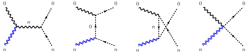
Figure 1: Scattering processes of zero-mode photon and longitudinally (scalar)-polarized KK graviton, $\,h_{n}^{L}A^{T}_{0}\!\rightarrow\!\SS^{-}_{0}\SS^{+}_{n}$ and $\,\tilde{h}_{n}^{S}A^{T}_{0}\!\rightarrow\!\SS^{-}_{0}\SS^{+}_{n}$, via the $(s,t,u)$-channels and contact interactions. Here the blue double-waved-line denotes the KK graviton $h_{n}^{\mu\nu}$, the black waved-line denotes zero-mode photon $A_{0}^{\mu}$ , and the black dashed line denotes the zero-mode scalar $\SS_{0}$ or KK scalar $\SS_{n}$.

We first compute the diagrams in Fig. 1 for the initial state with scalar-polarized KK graviton $\tilde{h}_{n}^{S}$ . Thus, the scattering amplitude is derived as

$$\mathcal{M}[\tilde{h}_{n}^{S}]\,=\,-\sqrt{\frac{3}{2}\,}e\kappa\,(\hskip 0.85358ptp_{3}\!\cdot\epsilon_{2}^{\pm})\,.$$ (2.3i)

Then, we consider the corresponding scattering amplitudes $\,\phi_{n}A^{T}_{0}\!\rightarrow\!\SS^{-}_{0}\SS^{+}_{n}$ and $\,\tilde{h}_{n}A^{T}_{0}\!\rightarrow\!\SS^{-}_{0}\SS^{+}_{n}$, as shown in Fig. 2. From Fig. 2, we compute the scattering amplitudes with initial state KK Goldstone boson $\phi_{n}$ and the unphysical trace-part of the KK graviton field $\tilde{h}_{n}$, respectively. We further derive their summed scattering amplitude. Now, these scattering amplitudes are presented as follows:

$$\mathcal{M}[\phi_{n}] =\frac{1}{2}\sqrt{\frac{2}{3}}\,e\kappa\,(\hskip 0.85358ptp_{3}\!\cdot\epsilon_{2}^{\pm})\,,\qquad\mathcal{M}[\tilde{h}_{n}]=2\sqrt{\frac{2}{3}}\,e\kappa\,(\hskip 0.85358ptp_{3}\!\cdot\epsilon_{2}^{\pm})\,,$$ (2.3ja)

$$\mathcal{M}[\,\overline{\Omega}_{n}] =\mathcal{M}[\phi_{n}]-\mathcal{M}[\tilde{h}_{n}]\,=\,-\sqrt{\frac{3}{2}}\,e\kappa\,(\hskip 0.85358ptp_{3}\!\cdot\epsilon_{2}^{\pm})\,,$$ (2.3jb)

where the notation $\,\overline{\Omega}_{n}\!=\phi_{n}\!-\tilde{h}_{n}$ was introduced in Eq.(2.3h). Inspecting the scalar-polarized KK graviton amplitude (2.3i) and the summed amplitude (2.3jb), we deduce an equality,

$$\mathcal{M}[\tilde{h}_{n}^{S}]\,=\,\mathcal{M}[\,\overline{\Omega}_{n}]\,,$$ (2.3k)

which explicitly verifies the GRET identity (2.3j). We also note that for the current scattering process, the $\overline{\Omega}_{n}$-amplitude contains contributions by both the gravitational KK Goldstone boson $\,\phi_{n}\,$ and the trace-part of the KK graviton $\,\tilde{h}_{n}\,$,  which are of the same order of magnitude. This shows an essential difference from the case of the pure KK gauge theories (without gravity), where for each longitudinal KK gauge boson $A_{n}^{L}$, its corresponding KK Goldstone boson is just given by the scalar component $A_{n}^{5}$ [8].

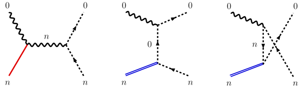
Figure 2: Scattering processes of the zero-mode photon and the KK gravitational Goldstone boson or the trace-part of KK graviton, $\,\phi_{n}A^{T}_{0}\!\!\rightarrow\!\SS^{-}_{0}\SS^{+}_{n}$ and $\,\tilde{h}_{n}A^{T}_{0}\!\!\rightarrow\!\SS^{-}_{0}\SS^{+}_{n}$ , via the $(s,t,u)$-channels, where the red solid-line denotes the KK gravitational scalar Goldstone $\phi_{n}$, the blue double-line denotes the trace-part of the KK graviton $\tilde{h}_{n}$.

Then, in order to compute the scattering amplitudes explicitly, we choose the momenta in the center-of-mass frame and make the initial state particles move along the $z$-axis. Then, the momenta for the initial state particles and final state particles are given by

$$p_{1}^{\mu}= -\!E(1,0,0,\beta), \hskip 28.45274ptp_{2}^{\mu}=-E\beta(1,0,0,-1),$$

$$p_{3}^{\mu}= \,E\beta(1,s_{\theta},0,c_{\theta}), \hskip 28.45274ptp_{4}^{\mu}=E(1,-\beta s_{\theta},0,-\beta c_{\theta}),$$ (2.3l)

where $\,\beta=\!\sqrt{1\!-\!M_{n}^{2}/E^{2}\,}$ and  $(s_{\theta},\,c_{\theta})\!=\!(\sin\theta,\,\cos\theta)$ with $\theta$ being the scattering angle. For simplicity of illustration, we consider the zero-mode mass $\,m_{0}\!\ll\!M_{n}$ and thus $\,m_{0}$  is negligible for this analysis. The polarization vectors of the KK graviton $h_{n}^{L}(p_{1})$ and zero-mode photon $A_{0}^{T}(p_{2})$ in the initial state take the following forms:

$$\varepsilon_{1L}^{\mu\nu} =\frac{1}{\sqrt{6\,}\,}(\epsilon^{\mu}_{1+}\epsilon^{\nu}_{1-}\!+\epsilon^{\mu}_{1-}\epsilon^{\nu}_{1+}\!+2\epsilon^{\mu}_{1L}\epsilon^{\nu}_{1L}),\leavevmode\nobreak\ \leavevmode\nobreak\ \leavevmode\nobreak\ \leavevmode\nobreak\ \epsilon^{\mu}_{1\pm}=\frac{1}{\sqrt{2\,}\,}(0,\pm 1,-\text{i},0),\leavevmode\nobreak\ \leavevmode\nobreak\ \leavevmode\nobreak\ \leavevmode\nobreak\ \leavevmode\nobreak\ \leavevmode\nobreak\$$

$$\epsilon_{1L}^{\mu} =-\frac{E}{M_{n}}(\beta,0,0,1),\leavevmode\nobreak\ \leavevmode\nobreak\ \quad\epsilon^{\mu}_{2\pm}=-\frac{1}{\sqrt{2\,}\,}(0,\pm 1,\text{i},0)\,.$$ (2.3m)

With the above, we compute explicitly the scattering amplitudes of $\,h_{n}^{L}A_{0}^{T}\!\!\rightarrow\!\SS^{-}_{0}\SS^{+}_{n}$ and $\,\tilde{h}_{n}^{S}A_{0}^{T}\!\rightarrow\!\SS^{-}_{0}\SS^{+}_{n}$ under the high energy expansion:

$$\mathcal{M}[h_{n}^{L}] \,=\,-\frac{5\sqrt{3}\,e\kappa}{6}(Es_{\theta})+\frac{\,\sqrt{3}\,e\kappa\,}{6}\frac{\,M_{n}^{2}(4\!-\!c_{\theta})\,}{\,E\tan(\theta/2)\,}+\mathcal{O}(E^{-3})\,,$$ (2.3na)

$$\mathcal{M}[\phi_{n}] \,=\,-\frac{\,\sqrt{3}\,e\kappa\,}{6}(Es_{\theta})+\frac{\,\sqrt{3}\,e\kappa\,}{12}\frac{\,M_{n}^{2}\,s_{\theta}\,}{E}+\mathcal{O}(E^{-3})\,,$$ (2.3nb)

where we have chosen the transverse polarization $\epsilon^{\mu}_{2+}$ for the initial state photon $A_{0}^{T}$.  For the other transverse polarization $\epsilon^{\mu}_{2-}$ of $A_{0}^{T}$,  all of the corresponding amplitudes will flip an overall sign.

According to the GRET identities (2.3j) and (2.3kb), we can compute the residual term:

$$\mathcal{M}[\widetilde{\Delta}_{n}]\,=\,\mathcal{M}[\tilde{v}_{n}]-\mathcal{M}[\tilde{h}_{n}]\,=\,\mathcal{M}[h_{n}^{L}]-\mathcal{M}[\phi_{n}]\,,$$ (2.3o)

where we have used the abbreviations $\,\mathcal{M}[\widetilde{\Delta}_{n}]\!\equiv\!\mathcal{M}[\widetilde{\Delta}_{n}A_{0}^{T}\!\!\rightarrow\!\SS^{-}_{0}\SS^{+}_{n}]$, $\,\mathcal{M}[\tilde{v}_{n}]\!\equiv\!\mathcal{M}[\tilde{v}_{n}A_{0}^{T}\!\!\rightarrow\!\SS^{-}_{0}\SS^{+}_{n}]$,  and $\,\mathcal{M}[\tilde{h}_{n}]\!\equiv\!\mathcal{M}[\tilde{h}_{n}A_{0}^{T}\!\!\rightarrow\!\SS^{-}_{0}\SS^{+}_{n}]\,$. Using the longitudinal KK graviton amplitude (2.3na) and KK Goldstone amplitude (2.3nb), we derive the residual term (2.3o) as follows:

$$\mathcal{M}[\widetilde{\Delta}_{n}]\,=\,-\frac{\,2\sqrt{3}\,e\kappa\,}{3}(Es_{\theta})+\mathcal{O}\!\left(\!\frac{M_{n}^{2}}{E}\right)\!,$$ (2.3p)

which has the same energy order as the longitudinal KK graviton amplitude $\mathcal{M}[h_{n}^{L}]$ . This demonstrates that for the case of one external KK graviton line, although the GRET identity (2.3k) holds as expected,

$$\mathcal{M}[h_{n}^{L}]\,=\,\mathcal{M}[\,\overline{\Omega}_{n}]+\mathcal{M}[\tilde{v}_{n}]\,=\,\mathcal{M}[\phi_{n}]+\mathcal{M}[\widetilde{\Delta}_{n}]\,,$$ (2.3q)

the GRET itself no longer holds. This is because the residual term $\,\mathcal{M}[\widetilde{\Delta}_{n}]\,$ in Eq.(2.3p) has the same order of magnitude as the longitudinal KK graviton amplitude $\,\mathcal{M}[h_{n}^{L}]\,$ or the KK Goldstone amplitude $\,\mathcal{M}[\phi_{n}]\,$ in Eq.(2.3n) under the high energy expansion.

Gravitational KK Goldstone Boson Scattering Amplitudes

In this subsection, we explicitly compute the elastic and inelastic scattering amplitudes of four gravitational KK Goldstone bosons in the compactified 5d GR, which will be compared quantitatively with the corresponding longitudinal (helicity-zero) KK graviton scattering amplitudes.

Elastic Gravitational KK Goldstone Boson Scattering Amplitudes

To compute the scattering amplitudes of the gravitational KK Goldstone bosons, we first derive the relevant interaction vertices. We will show that the leading contributions arise from the Feynman diagrams with zero-mode graviton and KK graviton exchanges. For the cubic interaction vertices containing one graviton and two KK scalar-Goldstone bosons, we expand EH Lagrangian up to $\mathcal{O}(\hat{\kappa}^{3})$, denoted as $\,\hat{\mathcal{L}}_{1}[\hat{h}\hat{\phi}^{2}]$ . We inspect the structure of $\,\hat{\mathcal{L}}_{1}[\hat{h}\hat{\phi}^{2}]$ and classify it into 12 Lorentz-invariant terms, as presented in Table 1.

$\hat{\mathcal{L}}_{1}[\hat{h}\hat{\phi}^{2}]$	$\hat{h}^{\mu\nu}\partial_{\mu}\hat{\phi}\,\partial_{\nu}\hat{\phi}$	$\hat{h}^{\mu\nu}\hat{\phi}\,\partial_{\mu}\partial_{\nu}\hat{\phi}$	$\hat{h}\,\partial_{\mu}\hat{\phi}\,\partial^{\mu}\hat{\phi}$	$\hat{h}\,\hat{\phi}\,\partial_{\mu}^{2}\hat{\phi}$	$\hat{h}\,\partial_{5}\hat{\phi}\,\partial^{5}\hat{\phi}$	$\hat{h}\,\hat{\phi}\,\partial_{5}^{2}\hat{\phi}$
	$\partial_{\mu}\hat{h}^{\mu\nu}\hat{\phi}\,\partial_{\nu}\hat{\phi}$	$(\partial_{\mu}\partial_{\nu}\hat{h}^{\mu\nu})\hat{\phi}^{2}$	$\partial_{\mu}\hat{h}\,\hat{\phi}\,\partial^{\mu}\hat{\phi}$	$(\partial_{\mu}^{2}\hat{h})\hat{\phi}^{2}$	$\partial_{5}\hat{h}\,\hat{\phi}\,\partial^{5}\hat{\phi}$	$(\partial_{5}^{2}\hat{h})\hat{\phi}^{2}$

Table 1: Classification of the 12 Lorentz-invariant interaction vertices in $\hat{\mathcal{L}}_{1}[\hat{h}\hat{\phi}^{2}]$, where the 6 operators in the second row (black color) can be converted into the combinations of the operators in the first row (red color) via integration by parts.

We note that in Table 1 all the 6 operators in the second row (black color) contain partial derivatives acting on the graviton fields, but we can always shift the partial derivatives on to the scalar fields via integration by parts, and thus they can be converted into combinations of the 6 operators in the first row (red color). In this way, we can organize the cubic vertices in the Lagrangian $\,\hat{\mathcal{L}}_{1}[\hat{h}\hat{\phi}^{2}]$  as follows:

$$\hat{\mathcal{L}}_{1}[\hat{h}\hat{\phi}^{2}]\,=\,\leavevmode\nobreak\ a_{1}\,\hat{h}^{\mu\nu}\partial_{\mu}\hat{\phi}\,\partial_{\nu}\hat{\phi}+a_{2}\,\hat{h}^{\mu\nu}\hat{\phi}\,\partial_{\mu}\partial_{\nu}\hat{\phi}+a_{3}\,\hat{h}(\partial_{\mu}\hat{\phi})^{2}+a_{4}\,\hat{h}\,\hat{\phi}\,\partial_{\mu}^{2}\hat{\phi}$$

$$+a_{5}\,\hat{h}(\partial_{5}\hat{\phi})^{2}+a_{6}\,\hat{h}\,\hat{\phi}\,\partial_{5}^{2}\hat{\phi}\,,$$ (2.3t)

where the coefficients are given by

$$(\hskip 0.85358pta_{1},\,a_{2},\,a_{3},\,a_{4},\,a_{5},\,a_{6}\hskip 0.85358pt)\,=\,\left(\!-\frac{1}{\,2\,},\,-1,\,\frac{3}{\,4\,},\,1,\,-\frac{1}{\,2\,},\,-\frac{1}{\,2\,}\hskip 0.85358pt\right)\!.$$ (2.3u)

Next, by substituting Eqs.(2.3la)-(2.3lc) into the Lagrangian (2.3t) and integrating over $x^{5}$, we derive the corresponding effective Lagrangian in 4d,

$$\mathcal{L}_{1}[h\phi^{2}]=\frac{\kappa}{\sqrt{2}}\sum_{n,m,\ell=1}^{\infty}\!\biggl{\{}\!$$

$$a_{1}\!\left[\!\sqrt{2}\left(h_{0}^{\mu\nu}\partial_{\mu}\phi_{0}\partial_{\nu}\phi_{0}+h_{0}^{\mu\nu}\partial_{\mu}\phi_{m}\partial_{\nu}\phi_{\ell}\delta_{m\ell}+h_{n}^{\mu\nu}\partial_{\mu}\phi_{m}\partial_{\nu}\phi_{0}\delta_{nm}+h_{n}^{\mu\nu}\partial_{\mu}\phi_{0}\partial_{\nu}\phi_{\ell}\delta_{n\ell}\right)\right.$$

$$\left.+\,h_{n}^{\mu\nu}\partial_{\mu}\phi_{m}\partial_{\nu}\phi_{\ell}\Delta_{3}(n,m,\ell)\right]+a_{2}\left[\!\sqrt{2}\left(h_{0}^{\mu\nu}\phi_{0}\partial_{\mu}\partial_{\nu}\phi_{0}+h_{0}^{\mu\nu}\phi_{m}\partial_{\mu}\partial_{\nu}\phi_{\ell}\delta_{m\ell}+h_{n}^{\mu\nu}\phi_{m}\partial_{\mu}\partial_{\nu}\phi_{0}\delta_{nm}\right.\right.$$

$$\left.\left.+\,h_{n}^{\mu\nu}\phi_{0}\partial_{\mu}\partial_{\nu}\phi_{\ell}\delta_{n\ell}\right)+h_{n}^{\mu\nu}\phi_{m}\partial_{\mu}\partial_{\nu}\phi_{\ell}\Delta_{3}(n,m,\ell)\right]+a_{3}\left[\,\!\!\sqrt{2}\left(h_{0}\partial_{\mu}\phi_{0}\partial^{\mu}\phi_{0}+h_{0}\partial_{\mu}\phi_{m}\partial^{\mu}\phi_{\ell}\delta_{m\ell}\right.\right.$$

$$\left.\left.+\,h_{n}\partial_{\mu}\phi_{m}\partial^{\mu}\phi_{0}\delta_{nm}+h_{n}\partial_{\mu}\phi_{0}\partial^{\mu}\phi_{\ell}\delta_{n\ell}\right)+h_{n}\partial_{\mu}\phi_{m}\partial^{\mu}\phi_{\ell}\Delta_{3}(n,m,\ell)\right]+a_{4}\left[\!\sqrt{2}\left(h_{0}\phi_{0}\partial^{2}_{\mu}\phi_{0}\right.\right.$$

$$\left.\left.+\,h_{0}\phi_{m}\partial^{2}_{\mu}\phi_{\ell}\delta_{m\ell}+h_{n}\phi_{m}\partial^{2}_{\mu}\phi_{0}\delta_{nm}+h_{n}\phi_{0}\partial^{2}_{\mu}\phi_{\ell}\delta_{n\ell}\right)+h_{n}\phi_{m}\partial^{2}_{\mu}\phi_{\ell}\Delta_{3}(n,m,\ell)\right]$$

$$+a_{5}M_{m}M_{\ell}\left[\,\!\!\sqrt{2}h_{0}\phi_{m}\phi_{\ell}\delta_{m\ell}h_{n}\phi_{m}\phi_{\ell}\widetilde{\Delta}_{3}(n,m,\ell)\!\,\right]-a_{6}M_{\ell}^{2}\left[\,\!\!\sqrt{2}\left(h_{0}\phi_{m}\phi_{\ell}\delta_{m\ell}+h_{n}\phi_{0}\phi_{\ell}\delta_{n\ell}\right)\right.$$

$$\left.+\,h_{n}\phi_{m}\phi_{\ell}\Delta_{3}(n,m,\ell)\,\right]\biggr{\}},$$ (2.3v)

where $\Delta_{3}(n,m,\ell)$ and $\widetilde{\Delta}_{3}(n,m,\ell)$ are given by

$$\Delta_{3}(n,m,\ell) \,=\,\delta(n+m-\ell)+\delta(n-m-\ell)+\delta(n-m+\ell)\,,$$ (2.3wa)

$$\widetilde{\Delta}_{3}(n,m,\ell) \,=\,\delta(n+m-\ell)-\delta(n-m-\ell)+\delta(n-m+\ell)\,.$$ (2.3wb)

Hence, using Eq.(2.3v), we can derive the Feynman rule for graviton-scalar-scalar interactions as shown in Fig. 3.

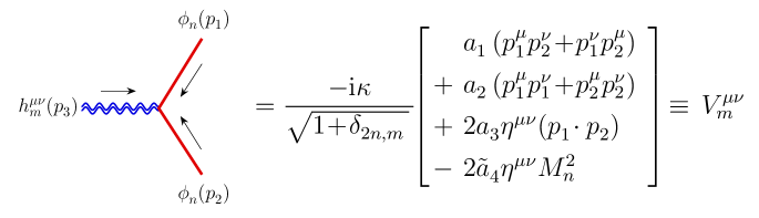
Figure 3: Feynman rule for the cubic interaction vertex between KK graviton and gravitational KK Goldstone bosons, where we define, $\,\tilde{a}_{4}=a_{4}+(-1)^{\delta_{2n,m}}a_{5}-a_{6}\hskip 0.85358pt$, with $m\!=0,\,2n$ .

With the above, we are ready to analyze the elastic scattering of the gravitational KK Goldstone bosons,  $\phi_{n}\phi_{n}\!\rightarrow\!\phi_{n}\phi_{n}$ . Fig. 4 shows the Feynman diagrams at the tree level, which include the scattering via the zero-mode graviton exchange and the KK graviton exchange at level-$2n$. By straightforward power counting, we find that each diagram in Fig. 4 has the leading contribution of $\,\mathcal{O}(E^{2})\,$ in the high energy limit. We stress that our gravitational KK Goldstone boson scattering amplitudes in our study do not invoke any energy cancellation among the individual diagrams and the leading energy dependence of $\mathcal{O}(E^{2})$ is manifest in each diagram. This feature is an essential difference from the longitudinal KK graviton amplitudes which involve a complicated large energy cancellations from $\mathcal{O}(E^{10})$ to $\mathcal{O}(E^{2})$ as in [14][15]. In fact, as we will demonstrate, our formulation of the GRET (section 3) together with the double-copy construction (section 5) can provide a general mechanism for these large energy cancellations.

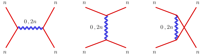
Figure 4: Elastic scattering of gravitational KK Goldstone bosons,  $\phi_{n}\phi_{n}\!\!\rightarrow\!\phi_{n}\phi_{n}$ , via $(s,\,t,\,u)$-channels mediated by the zero-mode graviton and by the KK graviton of level-$2n$.

By using the trilinear interaction vertices Fig. 3 and the KK graviton propagator (2.3va) as well as the kinematics defined in Appendix A, we can compute all the Feynman diagrams of Fig. 4 in a straightforward way. Summing up the individual diagrams, we derive the elastic scattering amplitude of  $\phi_{n}\phi_{n}\!\!\rightarrow\!\phi_{n}\phi_{n}$  to the leading order (LO) of $\mathcal{O}(E^{2})$ under the high energy expansion:

$$\mathcal{M}[\phi_{n}\phi_{n}\!\!\rightarrow\!\phi_{n}\phi_{n}] \leavevmode\nobreak\ =\leavevmode\nobreak\ \frac{\,3\kappa^{2}\,}{\,32}\!\left[\,\!\!\frac{\leavevmode\nobreak\ (3+\cos^{2}\!\theta)^{2}\,}{\sin^{2}\!\theta}\!\!\,\right]\!s_{0}\,,$$ (2.3xa)

$$\leavevmode\nobreak\ =\leavevmode\nobreak\ \frac{\,3\kappa^{2}\,}{\,128}\!\left[\,\!\!\frac{\leavevmode\nobreak\ (7\!+\cos 2\theta)^{2}\,}{\sin^{2}\!\theta}\!\!\,\right]\!s_{0}\,.$$ (2.3xb)

Then, the expansion to the next-to-leading order (NLO) gives the subleading amplitude:

$$\delta\mathcal{M}[\phi_{n}\phi_{n}\!\!\rightarrow\!\phi_{n}\phi_{n}]\,=\,-\frac{\,\kappa^{2}M_{n}^{2}\,}{128}(-1318+2865c_{2\theta}\!-522c_{4\theta}\!-c_{6\theta})\csc^{4}\!\theta\,,\hskip 28.45274pt$$ (2.3y)

which is mass-dependent contribution of $\,\mathcal{O}(E^{0}M_{n}^{2})\,$. We see that this NLO amplitude (2.3y) is much smaller than the LO amplitude (2.3x) of $\mathcal{O}(E^{2}M_{n}^{0})$ in the high energy scattering.

In order to explicitly demonstrate our GRET, we will first compare our gravitational KK Goldstone boson amplitude (2.3xb) with the corresponding longitudinal KK graviton amplitude $\mathcal{M}[h^{n}_{L}h^{n}_{L}\!\rightarrow\!h^{n}_{L}h^{n}_{L}]$ as given in Ref. [15] (cf. its Eq.(70)). For this comparison, we note a notational difference: our 4d gravitational coupling constant $\kappa$ is defined in Eq.(2.3g) as $\,\kappa\!=\!{\hat{\kappa}}/{\sqrt{L\,}}$  and differs from that of Ref. [15] by a factor  $\frac{\,{1}\,}{\sqrt{2}}$  since their definition leads to $\,\kappa\!=\!\hat{\kappa}/\!\sqrt{2L\,}$. Hence, our KK Goldstone amplitude (2.3xb) should be rescaled by a factor $\frac{\,{1}\,}{2}$ for the comparison:

$$\mathcal{M}\longrightarrow\mathcal{M}\times\frac{1}{2}=\frac{3\kappa^{2}}{\,256}\!\left[\,\!\!\frac{\,(7\!+\cos 2\theta)^{2}\,}{\sin^{2}\!\theta}\!\!\,\right]\!s_{0}\,,$$ (2.3z)

which equals the KK graviton amplitude in its Eq.(70) of Ref. [15]. This is truly impressive because our independent computation of the KK Goldstone amplitude (2.3xb) fully differs from that of the KK graviton amplitude which contains much more complicated energy cancellations from $\mathcal{O}(E^{10})$ to $\mathcal{O}(E^{2})$. Naively and intuitively, this equivalence seems quite expected for us because the scalar component of the KK graviton field $\,{\phi_{n}}\,(\equiv\!{h}^{55}_{n})$ should be converted to the degree of freedom of the helicity-zero longitudinal component of the KK graviton, and thus we would have

$$\mathcal{M}[h^{n}_{L}h^{n}_{L}\!\rightarrow\!h^{n}_{L}h^{n}_{L}]\,=\,\mathcal{M}[\phi_{n}\phi_{n}\!\!\rightarrow\!\phi_{n}\phi_{n}]+\mathcal{O}(M_{n}^{2}E^{0})\,.$$ (2.3aa)

However, in the actual situation it is far more nontrivial to quantitatively demonstrate the equivalence between the two amplitudes in the high energy limit. This is because our quantative formulation of the GRET (2.3c) (as systematically presented in section 3) shows that the second term on the RHS of the GRET contains a combination of both the KK Goldstone bosons $\,\phi_{n}\,$ and trace-part of graviton $\tilde{h}_{n}$  due to the structure of our $R_{\xi}$ gauge-fixing functions in Eqs.(2.3ab)-(2.3ac) and (2.3fa). To fully demonstrate such an equivalence as in Eq.(2.3aa), we have to further show that all the $\tilde{h}_{n}$-related Goldstone amplitudes on the RHS of the GRET (2.3c) together with the $\mathcal{O}(\tilde{v}_{n})$ amplitudes could be of $\mathcal{O}(M_{n}^{2}E^{0})$ at most. We will present this nontrivial demonstration in section 5 based on our double-copy construction.

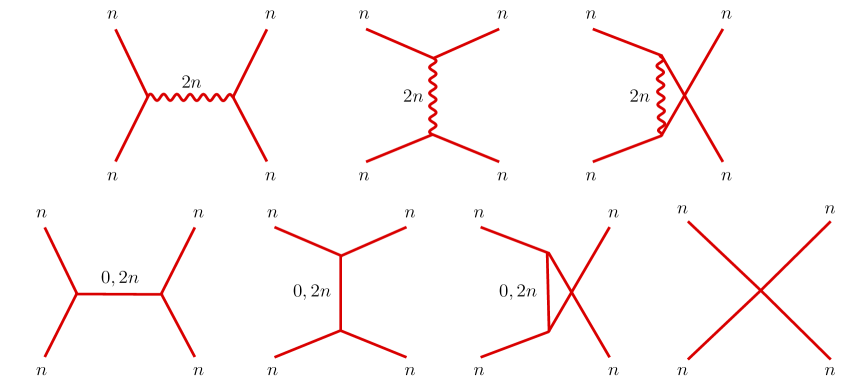
Figure 5: Gravitational KK Goldstone boson scattering $\,\phi_{n}\phi_{n}\!\!\rightarrow\!\phi_{n}\phi_{n}$ from Feynman diagrams of subleading contributions. The diagrams in the first row arise from exchanging the KK vector $\mathcal{A}_{2n}^{\mu}$ via $(s,t,u)$-channels, while the diagrams in the second row arise from exchanging both the zero-mode and KK scalar ($\phi_{0}\,,\phi_{2n}$) via $(s,t,u)$-channels and a KK scalar-Goldstone contact interaction.

Next, we compute the subleading contributions to the elastic KK Goldstone amplitude $\,\phi_{n}\phi_{n}\!\rightarrow\!\phi_{n}\phi_{n}\,$ as shown in Fig. 5, where the relevant Feynman rules are presented in Appendix D. These include the subleading contributions via $(s,t,u)$-channels mediated by a vector $\mathcal{A}_{2n}^{\mu}$ (the first row), a scalar $\phi_{0}$ or $\phi_{2n}$ (the second row), and a contact interaction (the second row). Thus, we derive the following three kinds of subleading contributions accordingly under the high energy expansion:

$$\mathcal{M}_{\mathcal{A}}[\phi_{n}\phi_{n}\!\rightarrow\!\phi_{n}\phi_{n}] \leavevmode\nobreak\ =\leavevmode\nobreak\ \frac{\,3\,}{4}\kappa^{2}M_{n}^{2}\,,$$ (2.3aba)

$$\mathcal{M}_{\phi}[\phi_{n}\phi_{n}\!\rightarrow\!\phi_{n}\phi_{n}] \leavevmode\nobreak\ =\leavevmode\nobreak\ -18\kappa^{2}M_{n}^{2}\,,$$ (2.3abb)

$$\mathcal{M}_{c}[\phi_{n}\phi_{n}\!\rightarrow\!\phi_{n}\phi_{n}] \leavevmode\nobreak\ =\leavevmode\nobreak\ \frac{\,9\,}{2}\kappa^{2}M_{n}^{2}\,.$$ (2.3abc)

Their sum is given by

$$\mathcal{M}_{\mathcal{A}}+\mathcal{M}_{\phi}+\mathcal{M}_{c}\,=\,-\frac{\,51\,}{4}\kappa^{2}M_{n}^{2}\,.$$ (2.3ac)

We see that the above subleading contributions are all of $\mathcal{O}(E^{0}M_{n}^{2})$. The same feature also holds for the subleading contributions to the inelastic channels.

Finally, we sum up the contributions of both Fig. 4 and Fig. 5, and derive the complete elastic scattering amplitude of KK scalar-Goldstone bosons without energy expansion:

$$\mathcal{M}[\phi_{n}\phi_{n}\!\!\rightarrow\!\phi_{n}\phi_{n}]\,=\,\frac{\,\kappa^{2}M_{n}^{2}(\widetilde{X}^{0}_{0}\!+\!\widetilde{X}^{0}_{2}c_{2\theta}\!+\!\widetilde{X}^{0}_{4}c_{4\theta}\!+\!\widetilde{X}^{0}_{6}c_{6\theta})}{\leavevmode\nobreak\ 512\bar{s}_{0}(\bar{s}_{0}\!+\!4)\left[\,2s_{\theta}^{2}\bar{s}_{0}^{2}\!+\!32\bar{s}_{0}\!+\!128\,\right]\!s_{\theta}^{2}\leavevmode\nobreak\ }\,,\hskip 28.45274pt$$ (2.3ad)

where $\,\bar{s}_{0}=s_{0}/M_{n}^{2}$ ,  $\bar{s}=s/M_{n}^{2}=\bar{s}_{0}\!+\!4\,$,  and

$$\widetilde{X}^{0}_{0} =2(255\bar{s}_{0}^{5}+\!13348\bar{s}_{0}^{4}+168624\bar{s}_{0}^{3}\!+\!984384\bar{s}_{0}^{2}+3514368\bar{s}_{0}+6012928)\hskip 0.85358pt,$$ (2.3aea)

$$\widetilde{X}^{0}_{2} =-429\bar{s}_{0}^{5}-12732\bar{s}_{0}^{4}-156288\bar{s}_{0}^{3}-777728\bar{s}_{0}^{2}-2572288\bar{s}_{0}-5210112\hskip 0.85358pt,$$ (2.3aeb)

$$\widetilde{X}^{0}_{4} =-2(39\bar{s}_{0}^{5}-1212\bar{s}_{0}^{4}-7824\bar{s}_{0}^{3}-10688\bar{s}_{0}^{2})\hskip 0.85358pt,$$ (2.3aec)

$$\widetilde{X}^{0}_{6} \,=\,-\left(3\bar{s}_{0}^{5}+\!4\bar{s}_{0}^{4}\right)\!.$$ (2.3aed)

From the above, we expand the full amplitude (2.3ad) $(\mathcal{M}[\phi_{n}\phi_{n}\!\!\rightarrow\!\phi_{n}\phi_{n}]\equiv\mathcal{M}[4\phi_{n}])$ down to the subleading order under the high energy expansion $\,s_{0}\!\gg\!M_{n}^{2}\,$ (or $\bar{s}_{0}\!\gg\!1$),

$$\mathcal{M}[4\phi_{n}] \,=\,\mathcal{M}_{0}[4\phi_{n}]+\delta\mathcal{M}[4\phi_{n}]\,,$$ (2.3afa)

$$\mathcal{M}_{0}[4\phi_{n}] \,=\,\frac{\,3\kappa^{2}\,}{\,128\,}\!\left[\,\!\!\frac{\,(7\!+\cos 2\theta)^{2}\,}{\sin^{2}\!\theta}\!\!\,\right]\!s_{0}\,,$$ (2.3afb)

$$\delta\mathcal{M}[4\phi_{n}] \,=\,-\frac{\,\kappa^{2}M_{n}^{2}\,}{128}(-706+2049c_{2\theta}\!-318c_{4\theta}\!-c_{6\theta})\csc^{4}\!\theta\,.$$ (2.3afc)

We see that the above leading amplitude $\,\mathcal{M}_{0}[4\phi_{n}]=\mathcal{O}(E^{2}M_{n}^{0})$  is mass-independent and agrees with Eq.(2.3x), while the subleading amplitude $\,\delta\mathcal{M}[4\phi_{n}]=\mathcal{O}(M_{n}^{2}E^{0})\,$ is mass-dependent. As a consistency check, we also note that the above subleading amplitude $\,\delta\mathcal{M}[4\phi_{n}]\,$ just equals the sum of the two NLO amplitudes (2.3y) and (2.3ac) which are computed earlier.

Inelastic Gravitational KK Goldstone Boson Scattering Amplitudes

In this subsection, we further analyze the inelastic scattering processes for the gravitational KK Goldstone bosons. Based on the analysis of the previous section, we have demonstrated that the longitudinal-Goldstone equivalence (2.3aa) holds down to $\mathcal{O}(E^{2})$ under the high energy expansion, which is equivalent to taking the high energy limit $\,M_{n}/E\!\rightarrow\!0$ .

From the trilinear interaction vertex Fig. 3, we can deduce a relation between the $\,h_{0}^{\mu\nu}$-$\phi_{n}$-$\phi_{n}\,$ coupling ($V^{\mu\nu}_{0}$) and $\,h_{2n}^{\mu\nu}$-$\phi_{n}$-$\phi_{n}\,$ coupling ($V^{\mu\nu}_{2n}$):

$$V^{\mu\nu}_{0}=\sqrt{2}\,V^{\mu\nu}_{2n}\,.$$ (2.3ag)

Thus, for each channel of the elastic scattering process, the corresponding amplitudes with the exchanges of zero-mode graviton $h_{0}^{\mu\nu}$ and KK graviton $h_{2n}^{\mu\nu}$ are connected by the relation: $\,\mathcal{M}_{j}^{2n}\!=\!\mbox{$\frac{\,{1}\,}{2}$}\mathcal{M}_{j}^{0}\,$.  Hence, for a given channel-$j$ , we have $\,\mathcal{M}_{j}\!=\mathcal{M}_{j}^{0}\!+\!\mathcal{M}_{j}^{2n}\!=\mbox{$\frac{\,{3}\,}{2}$}\mathcal{M}_{j}^{0}\,$ in the high energy limit $\,M_{n}/E\!\rightarrow\!0$ . With these, we can reproduce the elastic KK Goldstone scattering amplitude (2.3x) by

$$\mathcal{M}[\phi_{n}\phi_{n}\!\!\rightarrow\!\phi_{n}\phi_{n}]\,=\,\frac{3}{2}\,\sum_{j}\!\mathcal{M}_{j}^{0}\,,$$ (2.3ah)

where $\,j\in(s,\,t,\,u)$.  The above amplitude $\,\mathcal{M}_{j}^{0}\,$ arises from the exchange of zero-mode graviton and is given by

$$\mathcal{M}_{j}^{0}\leavevmode\nobreak\ =\,-\text{i}\,V_{\mu\nu}^{\,0}\,\mathcal{D}^{\mu\nu\alpha\beta}_{00}\,V_{\alpha\beta}^{\,0}\,.$$ (2.3ai)

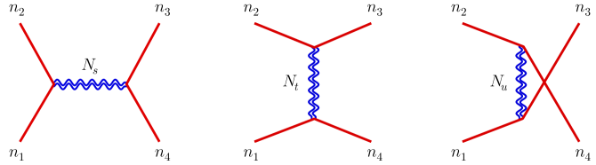
Figure 6: General four-point scattering process of the gravitational KK Goldstone bosons,  $\phi_{n_{1}}\phi_{n_{2}}\!\!\rightarrow\!\phi_{n_{3}}\phi_{n_{4}}$ , via $(s,\,t,\,u)$-channels mediated by a KK graviton of level $N_{s_{j}}$, where $N_{s_{j}}\!\!\geqslant 0$ and $s_{j}\in(s,t,u)$.

With the above, we can extend our analysis of the elastic scattering amplitude to a general case as shown in Fig. 6, including all the inelastic scattering channels. In Fig. 6, the external KK Goldstone bosons have KK-levels of $(n_{1},\,n_{2},\,n_{3},\,n_{4})$, and we denote the intermediate graviton with levels $(N_{s},\,N_{t},\,N_{u})\!\geqslant 0$, respectively.

In the following, we consider two types of the inelasic scattering processes:

1. For the inelasic scattering $\phi_{n}\phi_{n}\!\rightarrow\!\phi_{m}\phi_{m}$ (with $n\!\neq\!m$), we have

   $$n_{1}=n_{2}=n\,,\quad n_{3}=n_{4}=m\,,$$

   $$N_{s}=0\,,\quad N_{t}=N_{u}=|n\pm m|\,,$$ (2.3aj)

   where only the $s$-channel diagram includes the exchange of zero-mode graviton because of KK number conservation. With these, we compute the inelastic KK graviton scattering amplitude in the high energy limit as follows:

   $$\mathcal{M}[\phi_{n}\phi_{n}\!\rightarrow\!\phi_{m}\phi_{m}] \leavevmode\nobreak\ =\leavevmode\nobreak\ \mathcal{M}_{s}^{0}+2\times\mbox{$\frac{\,{1}\,}{2}$}\left(\mathcal{M}_{t}^{0}+\mathcal{M}_{u}^{0}\,\right)$$

   $$\leavevmode\nobreak\ =\leavevmode\nobreak\ \mbox{$\frac{\,{2}\,}{3}$}\,\mathcal{M}[\phi_{n}\phi_{n}\!\!\rightarrow\!\phi_{n}\phi_{n}]\,,$$ (2.3ak)

   where $\,\mathcal{M}_{j}^{0}\,$ is defined in Eq.(2.3ai) and equals the elastic amplitude of $\,h_{0}^{\mu\nu}$ exchange in the channel-$j$ .

2. For the inelasic scattering $\phi_{n}\phi_{k}\!\rightarrow\!\phi_{m}\phi_{\ell}$ (with $n\neq k\neq m\neq\ell$), we have

   $$n_{1}=n\,,\quad n_{2}=k\,,\quad n_{3}=m\,,\quad n_{4}=\ell\,,$$

   $$N_{s}=|n\pm k|=|m\pm\ell|\,,\quad N_{t}=|n\pm\ell|=|k\pm m|\,,\quad N_{u}=|n\pm m|=|k\pm\ell|\,.\quad$$ (2.3al)

   In this case, the process of exchanging zero-mode graviton is prohibited because of the KK number conservation, while the process by exchanging the relevant KK gravitons is allowed via $(s,\,t,\,u)$-channels. Thus, we have

   $$\mathcal{M}[\phi_{n}\phi_{k}\!\rightarrow\!\phi_{m}\phi_{\ell}] \leavevmode\nobreak\ =\leavevmode\nobreak\ \mbox{$\frac{\,{1}\,}{2}$}\left(\mathcal{M}_{s}^{0}+\mathcal{M}_{t}^{0}+\mathcal{M}_{u}^{0}\right)$$

   $$\leavevmode\nobreak\ =\leavevmode\nobreak\ \mbox{$\frac{\,{1}\,}{3}$}\,\mathcal{M}[\phi_{n}\phi_{n}\!\!\rightarrow\!\phi_{n}\phi_{n}]\,.$$ (2.3am)

As we checked, our above inelastic KK Goldstone boson amplitudes (2.3ak) and (2.3am) also equal the inelastic longitudinal KK graviton amplitudes [15] (cf. its Eq.(76)) after taking into account the notation difference.

Construction of Gravitational KK Amplitudes from Gauge KK Amplitudes with Double-Copy

In this section, we study the double-copy construction of the massive gravitational KK scattering amplitudes from the corresponding massive gauge KK scattering amplitudes under the high energy expansion. The conventional double-copy approaches (such as [24][25]) are realized for massless gauge theories and massless GR. The extension to the massive YM theory and massive Fierz-Pauli gravity is difficult without modification [44]. We stress that the KK YM gauge theory and KK GR are truly distinctive because they can consistently generate masses for KK gauge bosons and KK gravitons via geometric “Higgs” mechanism (under compactification) as shown in our sections 2-3 and in Refs. [8][9][12][13]. Hence, we expect that extending the conventional double-copy method to the KK theories should be truly promising even though highly challenging due to the KK mass-poles in the scattering amplitudes. Unlike the conventional double-copy approaches in the literature, we propose to realize the double-copy construction by using the high energy expansion order by order, and we will demonstrate explicitly how such a double-copy construction can work up to the leading order (LO) and the next-to-leading order (NLO). We are well motivated to use this high energy expansion approach for realizing the double-copy construction also because it perfectly matches our KK GAET and GRET formulations. So it should appropriately reconstruct the GRET based upon the KK GAET. Under the high energy expansion, we find that the LO KK gauge boson (Goldstone) amplitudes and KK graviton (Goldstone) amplitudes are mass-independent, so we can directly realize the double-copy construction of the LO KK amplitudes. Then, we show that the gauge and gravitational KK scattering amplitudes at the NLO are mass-dependent. We find that the double-copy construction for the mass-dependent NLO KK-amplitudes is highly nontrivial, where the conventional double-copy methods (such as BCJ [24][25]) could not fully work. We will present an improved BCJ-type double-copy construction for the KK gauge and gravitational amplitudes at the NLO.

In section 5.1, we will first analyze the structure of KK scattering amplitudes for the compactified 5d KK YM gauge theories without gravity. We present the exact tree-level four-particle scattering amplitudes of the KK longitudinal gauge bosons ($A_{L}^{an}$) and of the corresponding KK Goldstone bosons ($A_{5}^{an}$). With these, we analyze the structure of the KK $A_{L}^{an}$-amplitudes and KK $A_{5}^{an}$-amplitudes at both the LO and NLO under the high energy expansion. We show explicitly that the BCJ-type numerators hold the kinematic Jacobi identity for the LO KK-amplitudes, but the numerators of the NLO KK-amplitudes do not. Then, we show that the NLO numerators can be properly improved to obey the kinematic Jacobi identities. We also show explicitly how the KK equivalence theorem for gauge theory (KK GAET) [8] is realized in such KK YM gauge theories. Then, in section 5.2, we demonstrate that the scattering amplitudes of massive longitudinal KK gravitons ($h_{L}^{n}$) and the amplitudes of their KK Goldstone bosons ($\phi_{n}$) in the 5d KK GR can be reconstructed from the corresponding scattering amplitudes of the massive longitudinal KK gauge bosons and KK Goldstone bosons in the 5d KK YM gauge theory by using the double-copy method at the LO of the high energy expansion, where the reconstructed LO KK-amplitudes of $h_{L}^{n}$ and of $\phi_{n}$ have $\mathcal{O}(E^{2}M_{n}^{0})$ and are mass-independent. The reconstructed NLO gravitational KK-amplitudes have $\mathcal{O}(E^{0}M_{n}^{2})$ and are mass-dependent. We find that their double-copy construction is highly nontrivial. In section 5.3, we show that by direct extension of the double-copy method to the NLO KK amplitudes, we can reconstruct the correct kinematic structure of the KK $h_{L}^{n}$-amplitude and $\phi_{n}$-amplitude, but not their exact cofficients. For the difference between the $h_{L}^{n}$-amplitude and $\phi_{n}$-amplitude, such a naive extension fails to reproduce even the correct structure in the original gravitational amplitude-difference at the NLO. We will present an improved method to realize the correct structure of the NLO gravitational amplitude-difference, and then further demonstrate how to fully reconstruct the exact KK $h_{L}^{n}$-amplitude and $\phi_{n}$-amplitude separately. In section 5.4, we apply the double-copy approach of sections 5.2-5.3 to reconstruct the residual term of the KK GRET and show it has $\mathcal{O}(E^{0}M_{n}^{2})$ and is indeed suppressed relatively to the leading KK Goldstone $\phi_{n}$-amplitude. In this way, we can build the KK GRET in the 5d KK GR theory from the KK GAET in the 5d KK YM gauge theory.

Structure of Amplitudes for KK Gauge Bosons and Goldstone Bosons

Consider a non-Abelian gauge group $\mathcal{G}$, such as $\mathcal{G}=\mathrm{SU(N)}$, with group structure constant $C^{abc}$. For convenience, we denote the products of two structure constants as

$$\left(\,\mathcal{C}_{s},\,\mathcal{C}_{t},\,\mathcal{C}_{u}\,\right)\equiv\left(C^{abe}C^{cde},\,C^{ade}C^{bce},\,C^{ace}C^{dbe}\right).$$ (2.3a)

Thus, the Jacobi identity for the group structure constants takes the following form:

$$\mathcal{C}_{s}+\mathcal{C}_{t}+\mathcal{C}_{u}\,=\,0\,.$$ (2.3b)

This maybe called the “color” Jacobi identity since it contains the gauge group’s structure constants only.

We compactify a 5d YM gauge theory on $S^{1}\!/\mathbb{Z}_{2}$. This 5d compactification leads to a geometric “Higgs” mechanism [8] for the KK gauge boson mass-generation, where the longitudinal KK gauge boson $A^{an}_{L}$ arises from absorbing the fifth component of the KK state $A^{an}_{5}$. We start with the elastic scattering of longitudinal KK gauge bosons $A^{an}_{L}A^{bn}_{L}\!\rightarrow\!A^{cn}_{L}A^{dn}_{L}$ and the elastic scattering of the corresponding KK Goldstone bosons $A^{an}_{5}A^{bn}_{5}\!\rightarrow\!A^{cn}_{5}A^{dn}_{5}$. For the KK Goldstone amplitude, we choose the Feynman-’t Hooft gauge under which each KK Goldstone boson $A^{an}_{5}$ has the same mass $M_{n}$ as the KK gauge boson $A^{an}_{\mu}$. In the center-of-mass frame of the four-particle elastic scattering, we recall the kinematic variables defined in Eq.(A.3):

$$s_{0} =4k^{2}\,,$$ (2.3ca)

$$t_{0} =-\frac{\,s_{0}\,}{2}(1+c_{\theta})\,,$$ (2.3cb)

$$u_{0} =-\frac{\,s_{0}\,}{2}(1-c_{\theta})\,,$$ (2.3cc)

where the on-shell condition $\,k^{2}\!=\!E^{2}\!-\!M_{n}^{2}\,$ and $\,k\!=\!|\vec{p}\,|$ . The notations $(s_{0},\,t_{0},\,u_{0})$ correspond to the massless limit whose sum obeys $\,s_{0}+t_{0}+u_{0}=0$ . They are connected to the Mandelstam variables of the massive case via $(s_{0},\,t_{0},\,u_{0})=(s\!-\!4M_{n}^{2},\,t,\,u)$, where $\,s\!+t\!+u=4M_{n}^{2}\,$. We choose the convention that the momenta of all external particles are outgoing and the external particle numbers (1,2,3,4) are arranged clockwise in the scattering plane.

For the longitudinal KK gauge boson scattering and the corresponding KK Goldstone boson scattering in 5d YM under $S^{1}\!/\mathbb{Z}_{2}$ , the leading tree-level scattering amplitudes were given before [8] under high energy expansion. For the current study, we have further computed the exact tree-level KK longitudinal gauge boson amplitude $\,\mathcal{T}[A^{an}_{L}A^{bn}_{L}\!\rightarrow\!A^{cn}_{L}A^{dn}_{L}]\!\equiv\!\mathcal{T}[4A_{L}^{n}]$  and KK Goldstone boson amplitude $\,\widetilde{\mathcal{T}}[A^{an}_{5}A^{bn}_{5}\!\rightarrow\!A^{cn}_{5}A^{dn}_{5}]\equiv\widetilde{\mathcal{T}}[4A_{5}^{n}]$  as follows:

$$\mathcal{T}[4A_{L}^{n}]\,=\leavevmode\nobreak\ \, g^{2}({\mathcal{C}_{s}\mathcal{K}_{s}}+{\mathcal{C}_{t}\mathcal{K}_{t}}+{\mathcal{C}_{u}\mathcal{K}_{u}})\,,$$ (2.3da)

$$\widetilde{\mathcal{T}}[4A_{5}^{n}]\,=\leavevmode\nobreak\ \, g^{2}({\mathcal{C}_{s}\widetilde{\mathcal{K}}_{s}}+{\mathcal{C}_{t}\widetilde{\mathcal{K}}_{t}}+{\mathcal{C}_{u}\widetilde{\mathcal{K}}_{u}})\,,$$ (2.3db)

where

$$\mathcal{K}_{s} \displaystyle=-\frac{\,(4\bar{s}^{2}_{0}\!+27\bar{s}_{0}\!+36)c_{\theta}\,}{2(\bar{s}_{0}\!+\!4)}\,, \widetilde{\mathcal{K}}_{s} \displaystyle=-\frac{\,(3\bar{s}_{0}\!+4)c_{\theta}\,}{2(\bar{s}_{0}\!+4)}\,,$$ (2.3ea)

$$\mathcal{K}_{t} \displaystyle=-\frac{\,Q_{0}\!+Q_{1}c_{\theta}\!+Q_{2}c_{2\theta}\!+Q_{3}c_{3\theta}\,}{\,4\bar{s}_{0}[8+\bar{s}_{0}(1\!+\!c_{\theta})](1\!+\!c_{\theta})\,}\,, \widetilde{\mathcal{K}}_{t} \displaystyle=\frac{\,\widetilde{Q}_{0}\!+\widetilde{Q}_{1}c_{\theta}\!+\widetilde{Q}_{2}c_{2\theta}\,}{\,4\bar{s}_{0}[8+\bar{s}_{0}(1\!+\!c_{\theta})](1\!+\!c_{\theta})\,}\,,$$ (2.3eb)

$$\mathcal{K}_{u} \displaystyle=\frac{\,Q_{0}\!-Q_{1}c_{\theta}\!+Q_{2}c_{2\theta}\!-Q_{3}c_{3\theta}\,}{\,4\bar{s}_{0}[8+\bar{s}_{0}(1\!-\!c_{\theta})](1\!-\!c_{\theta})\,}\,, \widetilde{\mathcal{K}}_{u} \displaystyle=-\frac{\,\widetilde{Q}_{0}\!-\widetilde{Q}_{1}c_{\theta}\!+\widetilde{Q}_{2}c_{2\theta}\,}{\,4\bar{s}_{0}[8+\bar{s}_{0}(1\!-\!c_{\theta})](1\!-\!c_{\theta})\,}\,,$$ (2.3ec)

with

$$\bar{s}_{0}=s_{0}/M_{n}^{2}\,,\leavevmode\nobreak\ \leavevmode\nobreak\ \leavevmode\nobreak\ \bar{s}=s/M_{n}^{2}=\bar{s}_{0}\!+\!4\,,\leavevmode\nobreak\ \leavevmode\nobreak\ \leavevmode\nobreak\ c_{2\theta}\!=\cos 2\theta\,,\leavevmode\nobreak\ \leavevmode\nobreak\ \leavevmode\nobreak\ c_{3\theta}\!=\cos 3\theta\,,\hskip 14.22636pt$$ (2.3fa)

$$Q_{0}=8\bar{s}_{0}^{3}\!+33\bar{s}_{0}^{2}\!-48\bar{s}_{0}-\!128\,,\leavevmode\nobreak\ \leavevmode\nobreak\ \leavevmode\nobreak\ \leavevmode\nobreak\ Q_{1}=2(7\bar{s}_{0}^{3}\!+40\bar{s}_{0}^{2}\!+64\bar{s}_{0})\,,$$ (2.3fb)

$$Q_{2}=8\bar{s}_{0}^{3}\!+51\bar{s}_{0}^{2}\!+32\bar{s}_{0}\!-128\,,\hskip 16.21805ptQ_{3}=2(\bar{s}^{3}_{0}\!+\!2\bar{s}_{0}^{2}\!-8\bar{s}_{0})\,,$$ (2.3fc)

$$\widetilde{Q}_{0}=15\bar{s}_{0}^{2}\!+\!144\bar{s}_{0}\!+\!256\,,\leavevmode\nobreak\ \leavevmode\nobreak\ \leavevmode\nobreak\ \leavevmode\nobreak\ \widetilde{Q}_{1}=4(3\bar{s}^{2}_{0}\!+\!4\bar{s}_{0})\,,\leavevmode\nobreak\ \leavevmode\nobreak\ \leavevmode\nobreak\ \leavevmode\nobreak\ \widetilde{Q}_{2}=-3\bar{s}_{0}^{2}\,.$$ (2.3fd)

We note that the scattering amplitudes (2.3da)-(2.3db) have the leading high-energy behavior of $\mathcal{O}(E^{0})$. We make the high energy expansion for the amplitudes (2.3d)-(2.3f) down to the subleading order:

$$\mathcal{T}[4A_{L}^{n}]=\mathcal{T}_{0L}\!+\delta\mathcal{T}_{L}\,, \widetilde{\mathcal{T}}[4A_{5}^{n}]\,=\widetilde{\mathcal{T}}_{05}\!+\delta\widetilde{\mathcal{T}}_{5}\,,$$ (2.3ga)

$$\mathcal{T}_{0L}=\,g^{2}({\mathcal{C}_{s}\mathcal{K}_{s}^{0}}+{\mathcal{C}_{t}\mathcal{K}_{t}^{0}}+{\mathcal{C}_{u}\mathcal{K}_{u}^{0}})\,,\hskip 28.45274pt \widetilde{\mathcal{T}}_{05}=\,g^{2}({\mathcal{C}_{s}\widetilde{\mathcal{K}}_{s}^{0}}+{\mathcal{C}_{t}\widetilde{\mathcal{K}}_{t}^{0}}+{\mathcal{C}_{u}\widetilde{\mathcal{K}}_{u}^{0}})\,,$$ (2.3gb)

$$\delta\mathcal{T}_{L}=\,g^{2}({\mathcal{C}_{s}\delta\mathcal{K}_{s}}+{\mathcal{C}_{t}\delta\mathcal{K}_{t}}+{\mathcal{C}_{u}\delta\mathcal{K}_{u}})\,,\quad \delta\widetilde{\mathcal{T}}_{5}=\,g^{2}({\mathcal{C}_{s}\delta\widetilde{\mathcal{K}}_{s}}+{\mathcal{C}_{t}\delta\widetilde{\mathcal{K}}_{t}}+{\mathcal{C}_{u}\delta\widetilde{\mathcal{K}}_{u}})\,,$$ (2.3gc)

where $\,(\mathcal{K}_{j},\,\widetilde{\mathcal{K}}_{j})=(\mathcal{K}_{j}^{0}\!+\!\delta\mathcal{K}_{j},\,\widetilde{\mathcal{K}}_{j}^{0}\!+\!\delta\widetilde{\mathcal{K}}_{j})$  are given by

$$\mathcal{K}_{s}^{0} \displaystyle\,=\,-\frac{\,11\,}{2}c_{\theta}\,, \widetilde{\mathcal{K}}_{s}^{0} \displaystyle\,=\,-\frac{3}{\,2\,}c_{\theta}\,,$$ (2.3ha)

$$\mathcal{K}_{t}^{0} \displaystyle\,=\,\frac{\,5-11c_{\theta}\!-4c_{2\theta}\,}{\,2(1\!+\!c_{\theta})\,}\,, \widetilde{\mathcal{K}}_{t}^{0} \displaystyle\,=\,\frac{\,3(3\!-\!c_{\theta})\,}{\,2(1\!+\!c_{\theta})\,}\,,$$ (2.3hb)

$$\mathcal{K}_{u}^{0} \displaystyle\,=\,-\frac{\,5+11c_{\theta}\!-4c_{2\theta}\,}{\,2(1\!-\!c_{\theta})\,}\,, \widetilde{\mathcal{K}}_{u}^{0} \displaystyle\,=\,-\frac{\,3(3\!+\!c_{\theta})\,}{\,2(1\!-\!c_{\theta})\,}\,;$$ (2.3hc)

and

$$\delta\mathcal{K}_{s} \displaystyle\,=\,\frac{\,4c_{\theta}\,}{\bar{s}_{0}}\,, \delta\widetilde{\mathcal{K}}_{s} \displaystyle\,=\,\frac{\,4c_{\theta}\,}{\bar{s}_{0}}\,,$$ (2.3ia)

$$\delta\mathcal{K}_{t} \displaystyle\,=\,\frac{\,2(2\!-\!3c_{\theta}\!-\!2c_{2\theta}\!-\!c_{3\theta})\,}{(1\!+\!c_{\theta})\,\bar{t}_{0}}\,, \delta\widetilde{\mathcal{K}}_{t} \displaystyle\,=\,-\frac{\,8c_{\theta}\,}{(1\!+\!c_{\theta})\,\bar{t}_{0}}\,,$$ (2.3ib)

$$\delta\mathcal{K}_{u} \displaystyle\,=\,-\frac{\,2(2\!+\!3c_{\theta}\!-\!2c_{2\theta}\!+\!c_{3\theta})\,}{(1\!-\!c_{\theta})\,\bar{u}_{0}}\,, \delta\widetilde{\mathcal{K}}_{u} \displaystyle\,=\,-\frac{\,8c_{\theta}\,}{(1\!-\!c_{\theta})\,\bar{u}_{0}}\,.$$ (2.3ic)

We note that the leading order amplitudes $\,\mathcal{K}_{j}^{0},\widetilde{\mathcal{K}}_{j}^{0}\!=\!\mathcal{O}(E^{0}M_{n}^{0})\,$ which are both energy-independent and mass-independent, while the subleading amplitudes $\,\delta\mathcal{K}_{j},\delta\widetilde{\mathcal{K}}_{j}=\mathcal{O}(M_{n}^{2}/E^{2})\,$ which will vanish in the high energy limit $M_{n}^{2}/E^{2}\!\rightarrow\!0$ .

Inspecting the leading amplitudes of $\mathcal{O}(E^{0}M_{n}^{0})$ as in Eq.(2.3gb) and Eqs.(2.3ia)-(2.3ic), we find that longitudinal KK gauge boson amplitude and KK Goldstone boson amplitude differ by the same amount in each channel:

$$\mathcal{K}_{s}^{0}-\widetilde{\mathcal{K}}_{s}^{0}\,=\,\mathcal{K}_{t}^{0}-\widetilde{\mathcal{K}}_{t}^{0}\,=\,\mathcal{K}_{u}^{0}-\widetilde{\mathcal{K}}_{u}^{0}\,=\,-4c_{\theta}\,,$$ (2.3j)

which has zero contribution to the scattering amplitude due to the color Jacobi identity (2.3b). Hence, we have explicitly demonstrated the longitudinal-Goldstone equivalence between the longitudinal KK gauge boson scattering amplitude and KK Goldstone boson scattering amplitude at the leading order:

$$\mathcal{T}_{0L}\leavevmode\nobreak\ =\leavevmode\nobreak\ \widetilde{\mathcal{T}}_{05}\,.$$ (2.3k)

We note that since our above leading amplitudes are obtained by the high energy expansion of $\,M_{n}^{2}/s_{0}$ , instead of $\,M_{n}^{2}/s$ , our present longitudinal KK amplitude $\,\mathcal{T}_{0L}\,$ differs from that of Ref. [8] [in its Eq.(17)] by a common term of $\,-8g^{2}c_{\theta}\,$ in each of the $(s,t,u)$ channels, whose contribution to the amplitude vanishes due to the Jacobi identity (2.3b). On the other hand, the leading KK Goldstone boson amplitude $\,\widetilde{\mathcal{T}}_{05}\,$ coincides with that of Ref. [8] [in its Eq.(21)]. This is because there is no extra energy-cancellation in the KK Goldstone boson amplitude and the leading Goldstone amplitude does not depend on the choice of the expansion parameter as $\,M_{n}^{2}/s_{0}$  or $M_{n}^{2}/s$ .

We note that the subleading amplitudes (2.3gc) and (2.3ia)-(2.3ic) are of $\mathcal{O}(M_{n}^{2}/E^{2})$. Thus, we deduce the KK longitudinal-Goldstone equivalence at the LO under the high energy expansion:

$$\mathcal{T}[A^{an}_{L}A^{bn}_{L}\!\rightarrow\!A^{cn}_{L}A^{dn}_{L}]\,=\,\widetilde{\mathcal{T}}[A^{an}_{5}A^{bn}_{5}\!\rightarrow\!A^{cn}_{5}A^{dn}_{5}]+\,\mathcal{O}(M_{n}^{2}/E^{2})\,,$$ (2.3l)

which coincides with the KK Equivalence Theorem (KK-ET) [8].

For the convenience of double-copy construction, we define the notations:

$$(\mathcal{N}_{s},\,\mathcal{N}_{t},\,\mathcal{N}_{u})\,=\,(s_{0}\hskip 0.4pt\mathcal{K}_{s},\,t_{0}\hskip 0.4pt\mathcal{K}_{t},\,u_{0}\hskip 0.4pt\mathcal{K}_{u})\,,$$ (2.3ma)

$$(\widetilde{\mathcal{N}}_{s},\,\widetilde{\mathcal{N}}_{t},\,\widetilde{\mathcal{N}}_{u})\,=\,(s_{0}\hskip 0.4pt\widetilde{\mathcal{K}}_{s},\,t_{0}\hskip 0.4pt\widetilde{\mathcal{K}}_{t},\,u_{0}\hskip 0.4pt\widetilde{\mathcal{K}}_{u})\,,$$ (2.3mb)

$$\mathcal{N}_{j}=\,\mathcal{N}_{j}^{0}\!+\delta\mathcal{N}_{j}=\,s_{0j}(\mathcal{K}_{j}^{0}\!+\delta\mathcal{K}_{j})\,,$$ (2.3mc)

$$\widetilde{\mathcal{N}}_{j}=\,\widetilde{\mathcal{N}}_{j}^{0}\!+\delta\widetilde{\mathcal{N}}_{j}=\,s_{0j}(\widetilde{\mathcal{K}}_{j}^{0}\!+\delta\widetilde{\mathcal{K}}_{j})\,,$$ (2.3md)

where $\,s_{0j}\!\in\!(s_{0},\,t_{0},\,u_{0})\,$ and $\,j\!\in\!(s,\,t,\,u)\,$. With these, we can reexpress the elastic KK longitudinal and Goldstone scattering amplitudes as follows:

$$\mathcal{T}[4A^{n}_{L}] \,=\,g^{2}\!\left(\!\frac{\,\mathcal{C}_{s}\mathcal{N}_{s}\,}{s_{0}}+\frac{\,\mathcal{C}_{t}\mathcal{N}_{t}\,}{t_{0}}+\frac{\,\mathcal{C}_{u}\mathcal{N}_{u}\,}{u_{0}}\!\right)\!,$$ (2.3na)

$$\widetilde{\mathcal{T}}[4A^{n}_{5}] \,=\,g^{2}\!\left(\!\frac{\,\mathcal{C}_{s}\widetilde{\mathcal{N}}_{s}\,}{s_{0}}+\frac{\,\mathcal{C}_{t}\widetilde{\mathcal{N}}_{t}\,}{t_{0}}+\frac{\,\mathcal{C}_{u}\widetilde{\mathcal{N}}_{u}\,}{u_{0}}\!\right)\!.$$ (2.3nb)

Inspecting the leading-order kinematic quantities $(\mathcal{N}^{0}_{s},\,\mathcal{N}^{0}_{t},\,\mathcal{N}^{0}_{u})$ and $(\widetilde{\mathcal{N}}^{0}_{s},\,\widetilde{\mathcal{N}}^{0}_{t},\,\widetilde{\mathcal{N}}^{0}_{u})$ as given Eqs.(2.3ma)-(2.3mb) and Eq.(2.3h), we find that they are mass-independent and satisfy the following kinematic Jacobi identities:

$$\mathcal{N}_{s}^{0}+\mathcal{N}_{t}^{0}+\mathcal{N}_{u}^{0} \,=\,0\,,$$ (2.3oa)

$$\widetilde{\mathcal{N}}_{s}^{0}+\widetilde{\mathcal{N}}_{t}^{0}+\widetilde{\mathcal{N}}_{u}^{0} \,=\,0\,.$$ (2.3ob)

We can compare the two types of Jacobi identities (2.3b) and (2.3o): the former depends on the color factor (group structure constants) and the latter depends on kinematics. Since our above kinematic Jacobi identities (2.3oa)-(2.3ob) are mass-independent, they bear a similarity with the conventional color-kinematics duality [24][25] which was constructed for the 4d massless YM gauge theory and massless GR.

Furthermore, we note that, because of the Jacobi identity (2.3b), the above amplitudes (2.3na)-(2.3nb) are invariant under the shift:

$$\mathcal{N}_{j}\,\longrightarrow\,\mathcal{N}_{j}^{\,\prime}=\mathcal{N}_{j}+\Delta\!\times\!s_{0j}\,,$$ (2.3p)

where $\,\Delta\,$ is an arbitrary local function of kinematics. This shift may be called a generalized gauge transformation since its form bears some similarity to the gauge transformation. From Eq.(2.3p), we deduce the sum relation for numerators, $\,\sum_{j}\mathcal{N}_{j}^{\,\prime}\!=\sum_{j}\mathcal{N}_{j}\hskip 0.85358pt$, due to the fact of $\,s_{0}+t_{0}+u_{0}\!=0\,$. This will no longer hold for our double-copy construction under the $\hskip 0.85358pt1/s\hskip 0.85358pt$ expansion in section 5.3.2 because of $\hskip 0.85358pts+t+u=4M_{n}^{2}\,$.

Then, we compare the formulas of the leading KK longitudinal and Goldstone boson amplitudes in Eq.(2.3h) and Eqs.(2.3mc)-(2.3md). With these we derive the following relations between the two sets of kinematic quantities $(\mathcal{N}_{s}^{0},\,\mathcal{N}_{t}^{0},\,\mathcal{N}_{u}^{0})$ and $(\widetilde{\mathcal{N}}_{s}^{0},\,\widetilde{\mathcal{N}}_{t}^{0},\,\widetilde{\mathcal{N}}_{u}^{0})\hskip 0.85358pt$:

$$\mathcal{N}_{s}^{0}\,=\,\widetilde{\mathcal{N}}_{s}^{0}\!-4\hskip 0.85358ptc_{\theta}\hskip 0.85358pts_{0}\,,\leavevmode\nobreak\ \leavevmode\nobreak\ \leavevmode\nobreak\ \leavevmode\nobreak\ \mathcal{N}_{t}^{0}\,=\,\widetilde{\mathcal{N}}_{t}^{0}\!-4\hskip 0.85358ptc_{\theta}\hskip 0.85358ptt_{0}\,,\leavevmode\nobreak\ \leavevmode\nobreak\ \leavevmode\nobreak\ \leavevmode\nobreak\ \mathcal{N}_{s}^{0}\,=\,\widetilde{\mathcal{N}}_{u}^{0}\!-4\hskip 0.85358ptc_{\theta}\hskip 0.85358ptu_{0}\,.$$ (2.3q)

The above relations (2.3q) show that the leading longitudinal KK gauge boson scattering amplitude in Eq.(2.3na) and the leading KK Goldstone boson scattering amplitude in Eq.(2.3nb) differ by an amount $\,-4g^{2}c_{\theta}(\mathcal{C}_{s}+\mathcal{C}_{t}+\mathcal{C}_{u})$,  which vanishes identically due to the Jacobi identity (2.3b). As we noted earlier, this realizes the KK GAET as in Eq.(2.3k) or (2.3l).

We can further extend the above analysis to general processes including the inelastic KK scattering channels $A^{an}_{L}A^{bk}_{L}\!\rightarrow\!A^{cm}_{L}A^{d\ell}_{L}$  and $A^{an}_{5}A^{bk}_{5}\!\rightarrow\!A^{cm}_{5}A^{d\ell}_{5}$ , where the KK numbers of the initial and final states obey the condition $|n\!\pm\!k|=|m\!\pm\!\ell|$ . For this, we derive the following relations under the high energy expansion:

$$\mathcal{T}\!\left[\,\!A^{an}_{L}A^{bk}_{L}\!\rightarrow\!A^{cm}_{L}A^{d\ell}_{L}\,\right] \,=\,\zeta_{nkm\ell}\mathcal{T}\!\left[\,\!A^{an}_{L}A^{bn}_{L}\!\rightarrow\!A^{cn}_{L}A^{dn}_{L}\!\,\right]+\mathcal{O}(M_{j}^{2}/E^{2})\,,$$ (2.3ra)

$$\widetilde{\mathcal{T}}\!\left[\,\!A^{an}_{5}A^{bk}_{5}\!\rightarrow\!A^{cm}_{5}A^{d\ell}_{5}\,\right] \,=\,\zeta_{nkm\ell}\widetilde{\mathcal{T}}\!\left[\,\!A^{an}_{5}A^{bn}_{5}\!\rightarrow\!A^{cn}_{5}A^{dn}_{5}\!\,\right]+\mathcal{O}(M_{j}^{2}/E^{2})\,,$$ (2.3rb)

where $\,\zeta_{nnnn}\!=\!1\,$, $\,\zeta_{nnmm}\!=\!\mbox{$\frac{\,{2}\,}{3}$}\,$ for $n\!\neq\!m$ ,  and $\,\zeta_{nkm\ell}\!=\!\mbox{$\frac{\,{1}\,}{3}$}\,$ for the cases where the KK numbers $(n,k,m,\ell)$ have no more than one equality. From the above, we derive the KK GAET for general scattering processes including inelastic channels:

$$\mathcal{T}\!\left[\,\!A^{an}_{L}A^{bk}_{L}\!\rightarrow\!A^{cm}_{L}A^{d\ell}_{L}\,\right]=\widetilde{\mathcal{T}}\!\left[\,\!A^{an}_{5}A^{bk}_{5}\!\rightarrow\!A^{cm}_{5}A^{d\ell}_{5}\,\right]+\mathcal{O}(M_{j}^{2}/E^{2})\,,$$ (2.3s)

where the KK GAET for the elastic channel ($\,n\!=\!k\!=\!m\!=\!\ell\,$) and the inelastic channel ($\,n\!=\!k\neq m\!=\!\ell$ ) were demonstrated in Ref. [8].

Next, we examine the subleading amplitudes in Eqs.(2.3ia)-(2.3ic) and Eqs.(2.3mc)-(2.3md). From these, we derive

$$\sum_{j}\delta\mathcal{N}_{j}\,=\,\sum_{j}\delta\widetilde{\mathcal{N}}_{j}\,=\,\chi\,,$$ (2.3ta)

$$\chi\,=-2(7\!+c_{2\theta})c_{\theta}\csc^{2}\!\theta\,M_{n}^{2}\,,$$ (2.3tb)

where $\,j\!\in\!(s,\,t,\,u)\,$. We note that the next-to-leading-order (NLO) sums of $\delta\mathcal{N}_{j}$ and $\delta\widetilde{\mathcal{N}}_{j}$ are equal and do not vanish. Then, we compute the differences of the NLO numerators $\,(\delta\mathcal{N}_{j}-\delta\widetilde{\mathcal{N}}_{j})\,$ as follows:

$$\delta\mathcal{N}_{s}\!-\delta\widetilde{\mathcal{N}}_{s}=\,0\,,\leavevmode\nobreak\ \leavevmode\nobreak\ \leavevmode\nobreak\ \leavevmode\nobreak\ \leavevmode\nobreak\ \delta\mathcal{N}_{t}\!-\delta\widetilde{\mathcal{N}}_{t}=\,8s_{\theta}^{2}M_{n}^{2}\,,\leavevmode\nobreak\ \leavevmode\nobreak\ \leavevmode\nobreak\ \leavevmode\nobreak\ \leavevmode\nobreak\ \delta\mathcal{N}_{u}\!-\delta\widetilde{\mathcal{N}}_{u}=\,-8s_{\theta}^{2}M_{n}^{2}\,.$$ (2.3u)

From the above results, we find that the sum of the differences of these NLO numerators obeys a Jacobi identity:

$$\sum_{j}(\delta\mathcal{N}_{j}\!-\delta\widetilde{\mathcal{N}}_{j})=\,0\,.$$ (2.3v)

This property is important for us to understand the structure of the residual term in the GRET (2.3o) or (2.3p), as will be shown in section 5.2. Using (2.3u) and from Eqs.(2.3ga)(2.3n), we also derive the NLO amplitude difference:

$$\delta\mathcal{T}_{L}-\delta\widetilde{\mathcal{T}}_{5}\leavevmode\nobreak\ =\leavevmode\nobreak\ 8g^{2}s_{\theta}^{2}M_{n}^{2}\left(\frac{\,\mathcal{C}_{t}\,}{t_{0}}-\frac{\,\mathcal{C}_{u}\,}{u_{0}}\right)\!.$$ (2.3w)

As an extension, we may make two possible re-decompositions of the sum $\chi$ into the $(s,t,u)$ channels:

$$\chi\,\equiv\,\sum_{j}\chi_{j}\,\equiv\,\sum_{j}\widetilde{\chi}_{j}\,,$$ (2.3x)

where the kinematics hold the relations $\chi_{u}(\theta)=-\chi_{t}(\pi\!-\!\theta)$ and $\widetilde{\chi}_{u}(\theta)=-\widetilde{\chi}_{t}(\pi\!-\!\theta)$ . Then, we define the following modified subleading numerator factors:

$$\delta\mathcal{N}_{j}^{\prime}\,=\,\delta\mathcal{N}_{j}\!-\!\chi_{j}\,,\leavevmode\nobreak\ \leavevmode\nobreak\ \leavevmode\nobreak\ \leavevmode\nobreak\ \delta\widetilde{\mathcal{N}}_{j}^{\prime}\,=\,\delta\widetilde{\mathcal{N}}_{j}\!-\!\widetilde{\chi}_{j}\,,$$ (2.3y)

which keep Eq.(2.3v) invariant and satisfy the kinematic Jacobi identities separately:

$$\sum_{j}(\delta\mathcal{N}_{j}^{\prime}\!-\delta\widetilde{\mathcal{N}}_{j}^{\prime})=\,0\,,$$ (2.3za)

$$\sum_{j}\!\delta\mathcal{N}_{j}^{\prime}=0\,,\leavevmode\nobreak\ \leavevmode\nobreak\ \leavevmode\nobreak\ \leavevmode\nobreak\ \sum_{j}\!\delta\widetilde{\mathcal{N}}_{j}^{\prime}=0\,.$$ (2.3zb)

Thus, from Eq.(2.3n), we define the improved scattering amplitudes for the KK longitudinal gauge bosons and KK Goldstone bosons:

$$\mathcal{T}^{\prime}[4A^{n}_{L}] \,=\,g^{2}\!\left(\!\frac{\,\mathcal{C}_{s}\mathcal{N}_{s}^{\prime}\,}{s_{0}}+\frac{\,\mathcal{C}_{t}\mathcal{N}_{t}^{\prime}\,}{t_{0}}+\frac{\,\mathcal{C}_{u}\mathcal{N}_{u}^{\prime}\,}{u_{0}}\!\right)\!,$$ (2.3aaa)

$$\widetilde{\mathcal{T}}^{\prime}[4A^{n}_{5}] \,=\,g^{2}\!\left(\!\frac{\,\mathcal{C}_{s}\widetilde{\mathcal{N}}_{s}^{\prime}\,}{s_{0}}+\frac{\,\mathcal{C}_{t}\widetilde{\mathcal{N}}_{t}^{\prime}\,}{t_{0}}+\frac{\,\mathcal{C}_{u}\widetilde{\mathcal{N}}_{u}^{\prime}\,}{u_{0}}\!\right)\!.$$ (2.3aab)

We note that according to the Jacobi identities (2.3o) and (2.3zb), the improved numerators $\,\mathcal{N}_{j}^{\prime}=\mathcal{N}_{j}^{0}+\delta\mathcal{N}_{j}^{\prime}\,$ and $\,\widetilde{\mathcal{N}}_{j}^{\prime}=\widetilde{\mathcal{N}}_{j}^{0}+\delta\widetilde{\mathcal{N}}_{j}^{\prime}\,$ obey the kinematic Jacobi identities separately:

$$\mathcal{N}_{s}^{\prime}+\mathcal{N}_{t}^{\prime}+\mathcal{N}_{u}^{\prime} \,=\,0\,,$$ (2.3aba)

$$\widetilde{\mathcal{N}}_{s}^{\prime}+\widetilde{\mathcal{N}}_{t}^{\prime}+\widetilde{\mathcal{N}}_{u}^{\prime} \,=\,0\,.$$ (2.3abb)

Thus, the improved KK scattering amplitudes (2.3aba)-(2.3abb) exhibit all the nice features required by the conventional double-copy construction of BCJ-type [24][25]. We will present such a double-copy construction for the KK graviton scattering amplitudes and the GRET in the next subsection. For the subleading KK YM amplitudes and KK graviton amplitudes, our focus will be on the residual term $\,\mathcal{T}_{v}\,$ in the KK GAET identity and the residual term $\,\mathcal{M}_{\Delta}\,$ in the GRET identity, which can be expressed respectively as the difference between the NLO longitudinal KK amplitude and the corresponding NLO KK Goldstone amplitude:

$$\mathcal{T}_{v} \leavevmode\nobreak\ =\leavevmode\nobreak\ \delta\mathcal{T}_{L}-\delta\widetilde{\mathcal{T}}_{5}\,,$$ (2.3aca)

$$\mathcal{M}_{\Delta} \leavevmode\nobreak\ =\leavevmode\nobreak\ \delta\mathcal{M}-\delta\widetilde{\mathcal{M}}\,,$$ (2.3acb)

where we have used the notations $\,\delta\mathcal{M}\equiv\delta\mathcal{M}[4h_{L}^{n}]\,$ and $\,\delta\widetilde{\mathcal{M}}\equiv\delta\widetilde{\mathcal{M}}[4\phi_{n}]\,$. For deriving the above NLO KK GAET identity (2.3aca) and the NLO GRET identity (2.3acb), we have input the LO KK GAET identity (2.3k) and the LO GRET identity (F.7a). The modified NLO numerators in Eq.(2.3y) give the modified NLO amplitudes as follows:

$$\delta\mathcal{T}_{L}^{\prime} \leavevmode\nobreak\ =\leavevmode\nobreak\ \delta\mathcal{T}_{L}-\,\sum_{j}\frac{\,\mathcal{C}_{j}\chi_{j}\,}{s_{0j}}\,,$$ (2.3ada)

$$\delta\widetilde{\mathcal{T}}_{5}^{\prime} \leavevmode\nobreak\ =\leavevmode\nobreak\ \delta\widetilde{\mathcal{T}}_{5}-\,\sum_{j}\frac{\,\mathcal{C}_{j}\widetilde{\chi}_{j}\,}{s_{0j}}\,.$$ (2.3adb)

With the above, we can reexpress the NLO KK GAET identity (2.3aca) in the following form:

$$\mathcal{T}_{v}^{\prime}\leavevmode\nobreak\ =\leavevmode\nobreak\ \delta\mathcal{T}_{L}^{\prime}-\delta\widetilde{\mathcal{T}}_{5}^{\prime}\,,$$ (2.3ae)

where $\,\mathcal{T}_{v}^{\prime}\,$ denotes the modified residual term defined by $\,\mathcal{T}_{v}^{\prime}=\mathcal{T}_{v}-\sum_{j}\mathcal{C}_{j}(\chi_{j}-\widetilde{\chi}_{j})/s_{0j}\,$. We note that even though in Eq.(2.3ae) the NLO KK longitudinal and Goldstone amplitudes $(\delta\mathcal{T}_{L}^{\prime},\,\delta\widetilde{\mathcal{T}}_{5}^{\prime})$ are both modified as in Eq.(2.3ad), the residual term is also modified as $\,\mathcal{T}_{v}^{\prime}\,$ accordingly. Hence, the NLO KK GAET identity (2.3ae) is equivalent to its original form (2.3aca), which means that the gauge symmetry of the KK YM theory is still retained by the identity (2.3ae).

With the double-copy construction, we can justify the size of the GRET residual term $\,\mathcal{M}_{\Delta}\!=\mathcal{O}(M_{n}^{2}E^{0})\,$ from the KK GAET residual term $\,\mathcal{T}_{v}\!\!=\!\mathcal{O}(M_{n}^{2}/E^{2})\,$, where $\mathcal{T}_{v}$ is well understood. We will demonstrate that the connection between sizes of the two residual terms $\,\mathcal{T}_{v}\!=\!\mathcal{O}(M_{n}^{2}/E^{2})\,$ and $\,\mathcal{M}_{\Delta}\!\!=\!\mathcal{O}(M_{n}^{2}E^{0})\,$ is a general prediction of the double-copy construction and does not depend on details of the construction.

Constructing KK Scattering Amplitudes and GRET by Double-Copy

For the compactified 5d YM gauge theory and compactified 5d GR theory, we expect the double-copy correspondence:

$$A_{n}^{a\mu}\otimes\!A_{n}^{a\nu}\ \longrightarrow\,h^{\mu\nu}_{n}\,,$$ (2.3afa)

$$A_{n}^{a5}\otimes\!A_{n}^{a5}\ \longrightarrow\,h^{55}_{n}\,,$$ (2.3afb)

$$A_{n}^{a\mu}\otimes\!A_{n}^{a5}\ \longrightarrow\,h^{\mu 5}_{n}\,.$$ (2.3afc)

It is instructive to note that the physical spin-2 KK graviton field $h^{\mu\nu}_{n}$ arises from the double-copy of spin-1 KK gauge fields $A_{n}^{a\mu}\otimes\!A_{n}^{a\nu}$. On the other hand, the $A_{n}^{a5}$ is the would-be KK Goldstone boson in the compactified 5d YM gauge theory, and the double-copy counterparts $h^{55}_{n}(=\phi_{n})$ and $h^{\mu 5}_{n}$ just correspond to the scalar KK Goldstone boson and vector KK Goldstone boson in the compactified 5d GR. From Eq.(2.3afa) , we further expect the double-copy correspondence between the (helicity-zero) longitudinal KK graviton and KK gauge boson: $\,A_{L}^{an}\otimes\!A_{L}^{an}\!\longrightarrow h_{L}^{n}\,$. We observe that in the high energy limit the longitudinal KK gauge boson $A_{L}^{an}\!=\epsilon_{L}^{\mu}A^{an}_{\mu}\,$ has its polarization vector $\,\epsilon_{L}^{\mu}\!\!\sim\!k^{\mu}/M_{n}\,$, and the longitudinal KK graviton $\,h_{L}^{n}\!=\!\varepsilon_{L}^{\mu\nu}h^{n}_{\mu\nu}\,$ has its polarization tensor $\,\varepsilon_{L}^{\mu\nu}\!\!\sim\!k^{\mu}k^{\nu}/M_{n}^{2}\,$. Thus, we have $\,\varepsilon_{L}^{\mu\nu}\!\!\sim\!\epsilon_{L}^{\mu}\epsilon_{L}^{\nu}\,$ in the high energy limit, which also makes the longitudinal correspondence ($\,A_{L}^{an}\otimes\!A_{L}^{an}\!\longrightarrow h_{L}^{n}\,$) well expected. The demonstration of the double-copy correspondence between the longitudinal KK gauge boson amplitudes and the longitudinal KK graviton amplitudes is much more nontrivial than the above relation between the on-shell longitudinal polarization vector/tensor, as we will analyze further in this subsection.

In this subsection, we will first demonstrate that a double-copy construction from the KK gauge theory amplitudes to the KK graviton amplitudes at the leading order (LO) of the high energy expansion, which corresponds to the limit $\,M_{n}/E\!\rightarrow\!0\,$. We find that such leading order amplitudes are mass-independent and their kinematic Jacobi identities (2.3o) hold, in addition to the massless Mandelstam relation $\,s_{0}\!+t_{0}\!+u_{0}\!=0\,$. Thus, we will first extend the conventional double-copy method [24][25] to the LO amplitudes in our 5d KK theory and demonstrate how it works quantitatively.

We note that the (helicity-zero) longitudinal KK gauge bosons $A_{L}^{an}$ and longitudinal KK gravitons $h_{L}^{n}$ are truly distinctive in the KK theory because they do not exist in the commonly studied massless YM gauge theory or massless GR. Also, in the limit $M_{n}\!\rightarrow\!0$ , the KK Goldstone bosons $A_{5}^{an}$ and $\phi^{n}(=\!h^{n}_{55})$ both become massless and correspond to the physical degrees of freedom. But, it is important to observe that according to the KK GAET (cf. section 5.1) [8][9] and GRET (sections 3-4), the leading scattering amplitudes of the longitudinal KK gauge bosons (KK gravitons) equal the corresponding amplitudes of the KK Goldstone bosons and are mass-independent (which correspond to the limit $M_{n}^{2}/E^{2}\!\rightarrow\!0$  under high energy expansion). Hence, we can construct a double-copy from the leading longitudinal KK gauge boson amplitudes of $\mathcal{O}(E^{0})$ to the corresponding longitudinal KK graviton amplitudes of $\mathcal{O}(E^{2})$, in parallel to the double-copy construction between the KK Goldstone amplitudes in the KK YM theory and KK GR. The KK Goldstone amplitudes are much simpler due to the absence of any nontrivial energy-cancellations in the KK Goldstone amplitudes. Furthermore, since the compactified KK theories have very different Feynman rules from the 4d massless gauge theory or massless GR as commonly studied, the double-copy realization in the KK theory is far from obvious even for the leading order amplitudes before explicit demonstration. For instance, there are highly nontrivial and intricate energy-cancellations in the longitudinal KK gauge boson scattering amplitudes [from $\mathcal{O}(E^{4})$ down to $\mathcal{O}(E^{0}$)] [8] and in the (helicity-zero) longitudinal KK graviton scattering amplitudes [from $\mathcal{O}(E^{10})$ down to $\mathcal{O}(E^{2}$)] [15], all these do not exist in the 4d massless gauge theory and massless GR.

We inspect the structures of the KK longitudinal gauge boson scattering amplitude (2.3na) and the KK corresponding Goldstone boson scattering amplitude (2.3nb) in the compactified 5d YM gauge theory under the high energy expansion. We see from Eqs.(2.3g) and (2.3h)-(2.3i) that under high energy expansions, the leading amplitudes $(\mathcal{T}_{0L}\,,\,\widetilde{\mathcal{T}}_{05})$ are of $\,\mathcal{O}(E^{0})\,$ and mass-independent, while the subleading amplitudes $(\delta\mathcal{T}_{L}\,,\,\delta\widetilde{\mathcal{T}}_{5})$ are of $\,\mathcal{O}(M_{n}^{2}/E^{2})\,$ and vanish in the massless limit $M_{n}\!\rightarrow\!0$ . We have formally expressed these leading amplitudes in the form the massless gauge theories with pole factors $(s_{0},\,t_{0},\,u_{0})$ in the denominator of each channel, even though these poles are no longer real poles under the current high energy expansion. For the current study of the 5d KK YM gauge theories and 5d KK GR, we present an extended formulation of the conventional BCJ double-copy method of the massless gauge theories [24][25], by making the high energy expansion with $\,M_{n}^{2}/E^{2}\!\ll\!1$  under which all the nonzero KK mass-poles are removed, and the mass-dependent contributions can be treated order by order.

From the numerators of the amplitudes (2.3na)-(2.3nb), we see that the kinematic factors $(\mathcal{N}_{s},\,\mathcal{N}_{t},\,\mathcal{N}_{u})$ and $(\widetilde{\mathcal{N}}_{s},\,\widetilde{\mathcal{N}}_{t},\,\widetilde{\mathcal{N}}_{u})$ may be viewed as dual to the color factors $(\mathcal{C}_{s},\,\mathcal{C}_{t},\,\mathcal{C}_{u})$ according to the conventional double-copy method in the massless gauge theories [24][25]. Thus, we attempt to construct the elastic scattering amplitude $\,\mathcal{M}[h^{n}_{L}h^{n}_{L}\!\rightarrow\!h^{n}_{L}h^{n}_{L}]\,$ of the longitudinal KK gravitons and the gravitational KK Goldstone boson amplitude $\,\widetilde{\mathcal{M}}[\phi_{n}\phi_{n}\!\!\rightarrow\!\phi_{n}\phi_{n}]\,$ from the corresponding longitudinal KK gauge boson amplitude $\,\mathcal{T}[A^{an}_{L}A^{bn}_{L}\!\rightarrow\!A^{cn}_{L}A^{dn}_{L}]$  and the KK Goldstone boson amplitude $\,\widetilde{\mathcal{T}}[A^{an}_{5}A^{bn}_{5}\!\rightarrow\!A^{cn}_{5}A^{dn}_{5}]$,  respectively. We realize an extended double-copy construction for the 5d KK YM gauge theory and 5d KK GR by the following replacement:

$$(\mathcal{C}_{s},\,\mathcal{C}_{t},\,\mathcal{C}_{u})\ \longrightarrow\ (\mathcal{N}_{s},\,\mathcal{N}_{t},\,\mathcal{N}_{u})\,,$$ (2.3aga)

$$(\mathcal{C}_{s},\,\mathcal{C}_{t},\,\mathcal{C}_{u})\ \longrightarrow\ (\widetilde{\mathcal{N}}_{s},\,\widetilde{\mathcal{N}}_{t},\,\widetilde{\mathcal{N}}_{u})\,.$$ (2.3agb)

Applying this duality replacement to the scattering amplitudes of the longitudinal KK gauge bosons and KK Goldstone bosons in Eqs.(2.3na)-(2.3nb) and Eqs.(2.3h)(2.3mc)-(2.3md), we first construct the corresponding scattering amplitudes of the longitudinal KK gravitons and gravitational KK Goldstone bosons, to the nonzero leading contributions of $\mathcal{O}(E^{2})$ in the high energy expansion:

$$\mathcal{M}_{0}[h^{n}_{L}h^{n}_{L}\!\rightarrow\!h^{n}_{L}h^{n}_{L}]\, =c_{0}\,g^{2}\!\left[\,\!\frac{(\mathcal{N}_{s}^{0})^{2}}{s_{0}}+\frac{(\mathcal{N}_{t}^{0})^{2}}{t_{0}}+\frac{(\mathcal{N}_{u}^{0})^{2}}{u_{0}}\!\,\right]\!,$$ (2.3aha)

$$\widetilde{\mathcal{M}}_{0}[\phi_{n}\phi_{n}\!\!\rightarrow\!\phi_{n}\phi_{n}]\, =c_{0}\,g^{2}\!\left[\,\!\frac{(\widetilde{\mathcal{N}}_{s}^{0})^{2}}{s_{0}}+\frac{(\widetilde{\mathcal{N}}_{t}^{0})^{2}}{t_{0}}+\frac{(\widetilde{\mathcal{N}}_{u}^{0})^{2}}{u_{0}}\!\,\right]\!,$$ (2.3ahb)

where the overall coefficient $c_{0}$ is a conversion constant due to replacing the gauge coupling $\hskip 0.85358ptg\hskip 0.85358pt$ by gravitational coupling $\kappa$ . The constant $c_{0}$ is not known a priority before a unified UV theory of gauge and gravitational forces becomes available.

Then, substituting Eqs.(2.3ha)-(2.3hc) into Eqs.(2.3aha)-(2.3ahb), we explicitly reconstruct the longitudinal KK graviton scattering amplitude and the gravitational KK Goldstone scattering amplitude as follows:

$$\mathcal{M}_{0}[h^{n}_{L}h^{n}_{L}\!\rightarrow\!h^{n}_{L}h^{n}_{L}] =\widetilde{\mathcal{M}}_{0}[\phi_{n}\phi_{n}\!\!\rightarrow\!\phi_{n}\phi_{n}]$$

$$=\left(\!-\frac{\,9c_{0}g^{2}\,}{\,4\,}\!\right)\!\left[\,\!\frac{\,(3+\cos^{2}\!\theta)^{2}\,}{\sin^{2}\!\theta}\!\,\right]\!s_{0}$$ (2.3aia)

$$=\left(\!-\frac{\,9c_{0}g^{2}\,}{\,16\,}\!\right)\!\left[\left(7\!+\cos 2\theta\right)^{2}\!\csc^{2}\!\theta\,\right]\!s_{0}$$ (2.3aib)

$$=\left(\!-\frac{\,9c_{0}g^{2}\,}{\,4\,}\!\right)\!\!\left[\frac{\,(s_{0}^{2}+t_{0}^{2}+u_{0}^{2})^{2}\,}{s_{0}\hskip 1.5ptt_{0}\hskip 1.5ptu_{0}}\right]\!,$$ (2.3aic)

where we have dropped the mass-dependent subleading term of $\mathcal{O}(M_{n}^{2})$ which is much smaller than the above leading $\mathcal{O}(E^{2})$ amplitude in the high energy scattering.

Strikingly, we find that our above leading amplitudes of the longitudinal KK graviton and the gravitational KK Goldstone boson in Eq.(2.3ai), as constructed by the double-copy method, perfectly agree to the gravitational KK Goldstone amplitude (2.3x) at $\mathcal{O}(E^{2})$ which we computed directly from the KK theory of compactified 5d GR.

Eq.(2.3ai) also explicitly establishes the equivalence between the longitudinal KK graviton amplitude and the corresponding gravitational KK Goldstone boson amplitude. In fact, we can demonstrate this equivalence in a more elegant and transparent way, by making use of the relation (2.3q). With this, we can express the KK graviton amplitude (2.3aha) in terms of the gravitational KK Goldstone boson amplitude:

$$\mathcal{M}_{0}[h^{n}_{L}h^{n}_{L}\!\rightarrow\!h^{n}_{L}h^{n}_{L}]$$

$$=c_{0}g^{2}\!\left\{\!\left[\,\!\frac{(\widetilde{\mathcal{N}}_{s}^{0})^{2}}{s_{0}}\!+\!\frac{(\widetilde{\mathcal{N}}_{t}^{0})^{2}}{t_{0}}\!+\!\frac{(\widetilde{\mathcal{N}}_{u}^{0})^{2}}{u_{0}}\!\,\right]\!\!-8c_{\theta}(\widetilde{\mathcal{N}}_{s}^{0}\!+\widetilde{\mathcal{N}}_{t}^{0}\!+\widetilde{\mathcal{N}}_{u}^{0})\!+16c_{\theta}^{2}(s_{0}\!+t_{0}\!+u_{0})\right\}\hskip 28.45274pt$$

$$=\widetilde{\mathcal{M}}_{0}[\phi_{n}\phi_{n}\!\!\rightarrow\!\phi_{n}\phi_{n}],$$ (2.3aj)

where in the last step we have made use of the kinematic Jacobi identity (2.3ob) and the Mandelstam relation $\,s_{0}+t_{0}+u_{0}\!=0\,$. We see that the longitudinal KK graviton scattering amplitude equals the gravitational KK Goldstone scattering amplitude at the leading $\mathcal{O}(E_{n}^{2})$ and they differ only by subleading terms of $\mathcal{O}(E^{0}M_{n}^{2})$. The above Eq.(2.3aj) just demonstrates that the GRET holds for the longitudinal KK graviton scattering amplitude and the corresponding KK Goldstone scattering amplitude down to $\mathcal{O}(E^{2}M_{n}^{0})$ under the high energy expansion,

$$\mathcal{M}[h^{n}_{L}h^{n}_{L}\!\rightarrow\!h^{n}_{L}h^{n}_{L}]\,=\,\widetilde{\mathcal{M}}[\phi_{n}\phi_{n}\!\!\rightarrow\!\phi_{n}\phi_{n}]+\mathcal{O}(E^{0}M_{n}^{2})\,.$$ (2.3ak)

It is truly impressive to see that building upon the longitudinal-Goldstone equivalence of the KK GAET (2.3l) [or (2.3s)], we have established the corresponding longitudinal-Goldstone equivalence of the GRET for the amplitudes of the longitudinal KK graviton scattering and of the gravitational KK Goldstone scattering as in the above Eq.(2.3ak) by using the double-copy construction. Hence, this demonstrates a double-copy correspondence between the KK GAET in the compactified 5d YM gauge theory and the KK GRET in the compactified 5d GR.

We have the following comments in order:

1. Impressively, we find that our reconstructed gravitational KK Goldstone $\phi_{n}\,(=h^{55}_{n})$ amplitude $\widetilde{\mathcal{M}}_{0}[\phi_{n}\phi_{n}\!\!\rightarrow\!\phi_{n}\phi_{n}]$ in Eqs.(2.3ahb)(2.3ai) from the KK Goldstone $A_{5}^{an}$-amplitude $\widetilde{\mathcal{T}}_{0}[A^{an}_{5}A^{bn}_{5}\!\rightarrow\!A^{cn}_{5}A^{dn}_{5}]$ in Eqs.(2.3nb)(2.3ha)-(2.3hc) in the compactified 5d YM gauge theory via the double-copy approach has exactly the same energy and angular dependence as what we obtained by directly computing the $\phi_{n}$-amplitude (2.3x) in the compactified 5d KK GR theory. This double-copy reconstruction is naturally expected via the correspondence $\,A_{5}^{an}\otimes\!A_{5}^{an}\!\longrightarrow h_{55}^{n}\,$ where both the KK Goldstone bosons $A_{5}^{an}$ and $h^{n}_{55}(=\!\phi_{n})$ become effectively massless in the high energy limit $M_{n}^{2}/E^{2}\!\rightarrow\!0$ . We note that both the leading gravitational KK Goldstone amplitude (2.3ahb)(2.3ai) of $\mathcal{O}(E^{2})$ and the leading gauge-theory KK Goldstone amplitude (2.3nb)(2.3ha)-(2.3hc) of $\mathcal{O}(E^{0})$ are mass-independent. Hence, their structures reflect the 5d gauge symmetry of the KK YM theory and the 5d diffeomorphism invariance of the KK GR theory.

2. Note that the (helicity-zero) longitudinal KK gauge bosons $A_{L}^{an}$ and longitudinal KK gravitons $h_{L}^{n}$ do not exist in the massless YM gauge theory or massless GR. Hence they are truly distinctive in the KK theories. As we observe, the key point is that according to the KK GAET (section 5.1) [8][9] and GRET (sections 3-4), the leading longitudinal scattering amplitudes of $\,A_{L}^{an}\,$ and $\,h_{L}^{n}\,$ equal the corresponding amplitudes of the KK Goldstone bosons ($A_{5}^{an}$ and $h_{55}^{n}$) and are mass-independent (corresponding to the limit $M_{n}^{2}/E^{2}\!\rightarrow\!0$  under high energy expansion), despite that the longitudinal polarization vector $\epsilon_{L}^{\mu}$ (tensor $\varepsilon_{L}^{\mu\nu}$) of $A_{L}^{an}$ ($h_{L}^{n}$) has explicit mass-dependence. This is why we can construct a similar double-copy from the leading longitudinal KK gauge boson amplitudes of $\mathcal{O}(E^{0}M_{n}^{0})$ to the corresponding longitudinal KK graviton amplitudes of $\mathcal{O}(E^{2}M_{n}^{0})$. The above also explains that even though the original double-copy formulation [24][25] was shown to hold in the massless theory, we can still extend it to our current double-copy construction for the compactified massive KK theories to the leading order amplitude of $\mathcal{O}(E^{2}M_{n}^{0})$, which is mass-independent. All the mass-dependent terms belong to the subleading order of $\mathcal{O}(E^{0}M_{n}^{2})$ and are of the same order as the residual term in the GRET, as we will analyze further in sections 5.3-5.4.

   We stress that our double-copy construction guarantees that the leading longitudinal KK graviton (Goldstone) amplitude (2.3ah)-(2.3ai) must scale as $\,\mathcal{O}(E^{2}M_{n}^{0})\,$ under the high energy expansion. According to our double-copy construction, this $\,\mathcal{O}(E^{2}M_{n}^{0})\,$ high energy behavior just corresponds to the  $\mathcal{O}(E^{0}M_{n}^{0})\,$ leading energy behavior of the KK gauge (Goldstone) boson amplitude (2.3n), which are both mass-independent. In fact, our double-copy construction (based on the scattering amplitudes of 5d YM gauge theory and the KK GAET [8][9]) gives an independent proof that the longitudinal KK graviton scattering amplitudes must have large energy-cancellations of $\mathcal{O}(E^{10})\!\rightarrow\!\mathcal{O}(E^{2})$. We achieve this by establishing a new correspondence between the two energy-cancellations of the four-particle longitudinal KK scattering amplitudes: $\,E^{4}\!\!\rightarrow\!E^{0}\,$ in the 5d KK YM theory (YM5) and $\,E^{10}\!\!\rightarrow\!E^{2}\,$ in the 5d KK GR (GR5). Here, with the double-copy construction, we use the first energy-cancellation of $\,E^{4}\!\!\rightarrow\!E^{0}\,$ (YM5) to deduce the second energy-cancellation of $\,E^{10}\!\!\rightarrow\!E^{2}\,$ (GR5). Thus, we may present schematically this new correspondence between the two energy-cancellations as follows:

   $$E^{4}\!\!\rightarrow\!E^{0}\,\mathrm{(YM5)}\leavevmode\nobreak\ \leavevmode\nobreak\ \Longrightarrow\leavevmode\nobreak\ \leavevmode\nobreak\ E^{10}\!\!\rightarrow\!E^{2}\,\mathrm{(GR5)}\,.$$ (2.3al)

   In passing, some recent literature on the double-copy construction for certain specific KK models appeared [45][46], in which [45] briefly discussed a scalar model compactified on $\mathbb{R}^{4}\!\times\!S^{1}$ with an extra spectral condition imposed on the KK mass-spectrum, and [46] discussed a KK inspired action with extra global U(1) symmetry to have certain special mass-condition for double-copy. But these special KK models differ from the standard KK theory with obifold $S^{1}\!/\mathbb{Z}_{2}$ in our study and their methods do not apply to our case, so they do not overlap with our current study.

3. Our reconstructed gravitational KK Goldstone boson scattering amplitude (2.3ahb)(2.3ai) by double-copy method is confirmed by our direct computation of the gravitational KK Goldstone amplitude in Eq.(2.3x), which also equals our reconstructed (helicity-zero) longitudinal KK graviton amplitude (2.3ai). In addition, we find that our longitudinal KK graviton amplitude in Eq.(2.3ai) as reconstructed from our longitudinal KK gauge boson amplitude (2.3na) has exactly the same energy and angular dependence as those obtained by direct Feynman-diagram calculations of the longitudinal KK graviton amplitudes in Refs. [14][15].

4. The amplitudes (2.3aha)-(2.3ahb) have no double poles, so its denominator should be proportional to the product $\,s_{0}\hskip 1.0ptt_{0}\hskip 1.0ptu_{0}\,$,  which is permutation invariant among $(s_{0},\,t_{0},\,u_{0})$. We note that for the elastic scattering $\,(n,n)\!\!\rightarrow\!\!(n,n)\,$, the above amplitude should be invariant under all possible permutations, so the structure of this amplitude should take the form of $\,(s_{0}\hskip 1.0ptt_{0}\hskip 1.0ptu_{0})^{a}(s_{0}^{2}\!+\!t_{0}^{2}\!+\!u_{0}^{2})^{b}\,$ with $(a,\,b)$ being certain integers. Since the denominator of the scattering amplitude should scale like $\,s_{0}\hskip 1.0ptt_{0}\hskip 1.0ptu_{0}\!\propto\!s_{0}^{3}\,$,  so we have $\,a=-1\,$. Note that the whole amplitude is expected to scale like $\mathcal{O}(s^{1})$,  so the numerator has to scale as $\mathcal{O}(s^{4})$ . This means that the only possibility for the numerator is to scale as $\,(s_{0}^{2}+t_{0}^{2}+u_{0}^{2})^{2}\,$ with $\,b\!=\!2\,$. With these, we can generally deduce that the kinematic structure of the amplitude (2.3ah) behaves as $\,(s_{0}^{2}\!+\!t_{0}^{2}\!+\!u_{0}^{2})^{2}/(s_{0}\hskip 1.0ptt_{0}\hskip 1.0ptu_{0})\,$,  which explains why our explicit construction should lead to the formula of (2.3aic) indeed.

5. The overall conversion constant $c_{0}$ in Eqs.(2.3ah)-(2.3ai) is undetermined by the double-copy construction itself, but is expected to be universal at least for each given spacetime dimension. To match our double-copy result (2.3ai) with the gravitational KK Goldstone amplitude (2.3x), we choose the following conversion constant:

   $$c_{0}\,=\,-\frac{\kappa^{2}}{\,24g^{2}\,}\,.$$ (2.3am)

   We also notice that in the traditional massless 4d theory, the graviton amplitude reconstructed from the BCJ double-copy can fully match the graviton amplitude in 4d massless GR with the conversion constant

   $$\tilde{c}_{0}\,=\,\frac{\kappa^{2}}{\,16g^{2}\,}\,.$$ (2.3an)

   Our definition of the group structure constant $C^{abc}$ differs from the group structure constant $f^{abc}$ of Refs.[24][25] by a simple normalization factor:

   $$C^{abc}=\frac{1}{\sqrt{2\,}\,}f^{abc}=-\frac{\text{i}}{\sqrt{2\,}\,}\text{Tr}\left([T^{a},T^{b}]\,T^{c}\right)\,,$$ (2.3ao)

   where $T^{a}$ is the generator of SU(N) group.

Next, we further extend the above analysis to general processes $A^{an}_{L}A^{bk}_{L}\!\rightarrow\!A^{cm}_{L}A^{d\ell}_{L}$  and $A^{an}_{5}A^{bk}_{5}\!\rightarrow\!A^{cm}_{5}A^{d\ell}_{5}$  including the inelastic KK scattering channels. According to the Eqs.(2.3na)-(2.3nb) and Eq.(2.3r), we write the LO inelastic scattering amplitudes as follows:

$$\mathcal{T}_{0}\!\left[\,\!A^{an}_{L}A^{bk}_{L}\!\rightarrow\!A^{cm}_{L}A^{d\ell}_{L}\,\right] =g^{2}\zeta_{nkm\ell}\!\left(\!\frac{\,\mathcal{C}_{s}\mathcal{N}_{s}^{0}\,}{s_{0}}+\frac{\,\mathcal{C}_{t}\mathcal{N}_{t}^{0}\,}{t_{0}}+\frac{\,\mathcal{C}_{u}\mathcal{N}_{u}^{0}\,}{u_{0}}\!\right)\!,$$ (2.3apa)

$$\widetilde{\mathcal{T}}_{0}\!\left[\,\!A^{an}_{5}A^{bk}_{5}\!\rightarrow\!A^{cm}_{5}A^{d\ell}_{5}\,\right] =g^{2}\zeta_{nkm\ell}\!\left(\!\frac{\,\mathcal{C}_{s}\widetilde{\mathcal{N}}_{s}^{0}\,}{s_{0}}+\frac{\,\mathcal{C}_{t}\widetilde{\mathcal{N}}_{t}^{0}\,}{t_{0}}+\frac{\,\mathcal{C}_{u}\widetilde{\mathcal{N}}_{u}^{0}\,}{u_{0}}\!\right)\!,$$ (2.3apb)

where $\,\zeta_{nnnn}\!\!=\!\!1\,$, $\,\zeta_{nnmm}\!=\!\mbox{$\frac{\,{2}\,}{3}$}\,$ for $n\!\neq\!m$ ,  and $\,\zeta_{nkm\ell}\!=\!\mbox{$\frac{\,{1}\,}{3}$}\,$ for $(n,k,m,\ell)$ having no more than one equality. Thus, using the color-kinematics duality relations (2.3aga)-(2.3agb) and up to an overall conversion constant $c_{0}$ , we can further reconstruct the general scattering amplitude of longitudinal KK gravitons and the scattering amplitude of the corresponding gravitational KK Goldstone bosons by using the following relations:

$$\mathcal{M}\!\left[\,\!h^{n}_{L}h^{k}_{L}\!\rightarrow\!h^{m}_{L}h^{\ell}_{L}\!\,\right] \,=\leavevmode\nobreak\ \zeta_{nkm\ell}\,\mathcal{M}\!\left[\,\!h^{n}_{L}h^{n}_{L}\!\rightarrow\!h^{n}_{L}h^{n}_{L}\!\,\right]+\mathcal{O}(E^{0}M_{j}^{2})\,,$$ (2.3aqa)

$$\widetilde{\mathcal{M}}\!\left[\,\!\phi_{n}\phi_{k}\!\rightarrow\!\phi_{m}\phi_{\ell}\!\,\right] \,=\leavevmode\nobreak\ \zeta_{nkm\ell}\,\widetilde{\mathcal{M}}[\phi_{n}\phi_{n}\!\!\rightarrow\!\phi_{n}\phi_{n}]+\mathcal{O}(E^{0}M_{j}^{2})\,.$$ (2.3aqb)

Then, using Eq.(2.3ak), we can deduce the GRET by double-copy reconstruction for the general scattering process:

$$\mathcal{M}\!\left[\,\!h^{n}_{L}h^{k}_{L}\!\rightarrow\!h^{m}_{L}h^{\ell}_{L}\!\,\right]\,=\,\widetilde{\mathcal{M}}\!\left[\,\!\phi_{n}\phi_{k}\!\rightarrow\!\phi_{m}\phi_{\ell}\!\,\right]+\mathcal{O}(E^{0}M_{j}^{2})\,,$$ (2.3ar)

where the KK numbers of the initial and final states obey $|n\!\pm\!k|=|m\!\pm\!\ell|$ .

We observe that our double-copy constructions in Eqs.(2.3ak) and (2.3ar) have explicitly established the KK GRET from the KK GAET (2.3l) and (2.3s): the leading amplitude of the longitudinal KK graviton scattering equals that of the gravitational KK Goldstone scattering at $\mathcal{O}(E^{2})$ (which is mass-independent) under the high energy expansion, and their difference is only of $\hskip 0.85358pt\mathcal{O}(E^{0}M_{n}^{2})\hskip 0.85358pt$. This means that in our general formulation of the KK GRET (2.3p) the sum of all the $\mathcal{O}(\widetilde{\Delta}_{n})$ residual terms must be of $\mathcal{O}(E^{0}M_{n}^{2})$, even though the naive power counting on their individual amplitudes containing one or more external state of $\,\tilde{v}_{n}(=\tilde{v}_{\mu\nu}h^{\mu\nu}_{n})$  or  $\tilde{h}_{n}(=\eta_{\mu\nu}\tilde{h}_{n}^{\mu\nu})$  gives $\mathcal{O}(E^{2})$. Hence, we deduce that the double-copy construction of the KK GRET identity (2.3o) from the KK GAET identity [9] in the KK YM gauge theory provides a new mechanism of energy cancellation from $\mathcal{O}(E^{2})$ down to $\mathcal{O}(E^{0})$ in the sum of all the $\mathcal{O}(\widetilde{\Delta}_{n})$ residual terms on the RHS of the KK GRET (2.3p). We will further demonstrate the realization of this new energy-cancellation mechanism of $\,E^{2}\!\rightarrow\!E^{0}\,$ for the residual terms of GRET in the next subsections.

Constructing Mass-Dependent KK Amplitudes from Double-Copy

In this subsection, we study the extended double-copy construction of the mass-dependent KK scattering amplitudes at the NLO. We will make two types of high energy expansions by using the expansion parameter $\hskip 0.85358pt1/s_{0}\hskip 0.85358pt$ or $\hskip 0.85358pt1/s\hskip 0.85358pt$, where the Mandelstam variable $\,s=s_{0}+4M_{n}^{2}\,$ for the four-point elastic KK amplitudes. As we will show, the advantage of the $\hskip 0.85358pt1/s_{0}\hskip 0.85358pt$ expansion is that it can automatically ensure that the LO numerators of the KK amplitudes are mass-independent, but then the mass-dependent NLO numerators cannot obey the kinematic Jacobi identity even after the generalized gauge-transformation due to $\,s_{0}+t_{0}+u_{0}=0\hskip 0.85358pt$ [cf. Eq.(A.3)]. So additional modifications are needed. In contrast, under the $\hskip 0.85358pt1/s\hskip 0.85358pt$ expansion the LO numerators of KK amplitudes depend only on the $\hskip 0.85358pts\hskip 0.85358pt$ and $\hskip 0.85358pt\theta\hskip 0.85358pt$ (where the mass-dependence is contained only in $\hskip 0.85358pts\hskip 0.85358pt$ via $\hskip 0.85358pts=s_{0}+4M_{n}^{2}\,$), and we can make the gauge-transformed numerators obey the kinematic Jacobi identity oredr by order in the $\hskip 0.85358pt1/s\hskip 0.85358pt$ expansion due to $\,s+t+u=4M_{n}^{2}\hskip 0.85358pt$ [cf. Eq.(A.2)]. Hence, the $\hskip 0.85358pt1/s\hskip 0.85358pt$ expansion is expected to realize the double-copy construction more successfully. In the following, we will present the extended double-copy constructions for the NLO massive KK amplitudes by using the high energy expansion of $\hskip 0.85358pt1/s_{0}\hskip 0.85358pt$ in section 5.3.1 and the high energy expansion of $\hskip 0.85358pt1/s\hskip 0.85358pt$ in section 5.3.2.

Double-Copy of NLO KK Amplitudes under $1/s_{0}$ Expansion

In section 5.2, we focused on the double-copy construction of the KK gravitational amplitudes (2.3aha)-(2.3ahb) at the leading order (LO) of the high energy expansion. For this subsection, we study the double-copy KK amplitudes (2.3na)-(2.3nb) of the 5d KK YM gauge theory up to the next-to-leading order (NLO) of the $\hskip 0.85358pt1/s_{0}\hskip 0.85358pt$ expansion. For this, we extend the reconstructed KK gravitational amplitudes (2.3aha)-(2.3ahb) as follows:

$$\mathcal{M}[4h_{L}^{n}] \leavevmode\nobreak\ =\leavevmode\nobreak\ c_{0}\,g^{2}\!\left[\,\frac{(\mathcal{N}_{s})^{2}}{s_{0}}+\frac{(\mathcal{N}_{t})^{2}}{t_{0}}+\frac{(\mathcal{N}_{u})^{2}}{u_{0}}\,\right]=\mathcal{M}_{0}+\delta\mathcal{M}\,,$$ (2.3asa)

$$\widetilde{\mathcal{M}}[4\phi_{n}] \leavevmode\nobreak\ =\leavevmode\nobreak\ c_{0}\,g^{2}\!\left[\,\frac{(\widetilde{\mathcal{N}}_{s})^{2}}{s_{0}}+\frac{(\widetilde{\mathcal{N}}_{t})^{2}}{t_{0}}+\frac{(\widetilde{\mathcal{N}}_{u})^{2}}{u_{0}}\,\right]=\widetilde{\mathcal{M}}_{0}+\delta\widetilde{\mathcal{M}}\,,$$ (2.3asb)

where the conversion constant $\,c_{0}\!\!=\!\!-{\kappa^{2}}/(24g^{2})\,$ is given by Eq.(2.3am), as determined by matching the corresponding leading order gravitational KK amplitude (2.3x). According to Eqs.(2.3mc)-(2.3md), we expand the numerator factors $(\mathcal{N}_{j},\,\widetilde{\mathcal{N}}_{j})$ to the NLO and naively derive the following reconstructed subleading order gravitational KK amplitudes:

$$\delta\mathcal{M} \,=\leavevmode\nobreak\ 2c_{0}\,g^{2}\!\left(\frac{\mathcal{N}_{s}^{0}\delta\mathcal{N}_{s}}{s_{0}}+\frac{\mathcal{N}_{t}^{0}\delta\mathcal{N}_{t}}{t_{0}}+\frac{\mathcal{N}_{u}^{0}\delta\mathcal{N}_{u}}{u_{0}}\right)\!,$$ (2.3ata)

$$\delta\widetilde{\mathcal{M}} \,=\leavevmode\nobreak\ 2c_{0}\,g^{2}\!\left(\frac{\widetilde{\mathcal{N}}_{s}^{0}\delta\widetilde{\mathcal{N}}_{s}}{s_{0}}+\frac{\widetilde{\mathcal{N}}_{t}^{0}\delta\widetilde{\mathcal{N}}_{t}}{t_{0}}+\frac{\widetilde{\mathcal{N}}_{u}^{0}\delta\widetilde{\mathcal{N}}_{u}}{u_{0}}\right)\!.$$ (2.3atb)

We first note that the above double-copy construction should give the correct powers of the (energy, mass)-dependence of the corresponding NLO gravitational KK amplitudes under the high energy expansion. The structure of the KK amplitudes in the 5d KK YM gauge theory has been well understood as we showed in Eqs.(2.3d)-(2.3i) and Eqs.(2.3m)-(2.3n) of section 5.1. We see that in the 5d KK YM gauge theory, the LO and NLO amplitudes in each channel are $(\mathcal{K}_{j}^{0},\,\widetilde{\mathcal{K}}_{j}^{0})\!=\mathcal{O}(E^{0}M_{n}^{0})$ and $(\delta\mathcal{K}_{j},\,\delta\widetilde{\mathcal{K}}_{j})\!=\mathcal{O}(M_{n}^{2}/E^{2})$. Thus, the LO and NLO numerators are $(\mathcal{N}_{j}^{0},\,\widetilde{\mathcal{N}}_{j}^{0})=\mathcal{O}(E^{2}M_{n}^{0})$ and $(\delta\mathcal{N}_{j},\,\delta\widetilde{\mathcal{N}}_{j})=\mathcal{O}(E^{0}M_{n}^{2})$. Hence, we generally deduce that the reconstructed double-copy of the LO and NLO KK amplitudes for gravitational KK scattering should have the following power-dependence on the (energy, mass):

$$(\mathcal{M}_{0},\,\widetilde{\mathcal{M}}_{0}) \,=\,\mathcal{O}\!\left(\!\kappa^{2}\frac{\,(\mathcal{N}_{j}^{0})^{2}\!,\,(\widetilde{\mathcal{N}}_{j}^{0})^{2}\,}{s_{0j}}\!\right)=\,\mathcal{O}\!\left(\kappa^{2}E^{2}M_{n}^{0}\right)\!,$$ (2.3aua)

$$(\delta\mathcal{M},\,\delta\widetilde{\mathcal{M}}) \,=\,\mathcal{O}\!\left(\!\kappa^{2}\frac{\,\mathcal{N}_{j}^{0}\delta\mathcal{N}_{j},\,\widetilde{\mathcal{N}}_{j}^{0}\delta\widetilde{\mathcal{N}}_{j}\,}{s_{0j}}\!\right)=\,\mathcal{O}\!\left(\kappa^{2}E^{0}M_{n}^{2}\right)\!,$$ (2.3aub)

where $\,s_{0j}\!\in\!(s_{0},t_{0},u_{0})\!=\!\mathcal{O}(E^{2})\,$ and we have used $\,c_{0}g^{2}\sim\!\mathcal{O}(\kappa^{2})$ according to Eq.(2.3am). The above power counting fully agrees with the explicit calculations of the KK graviton (Goldstone) amplitudes of the compactified 5d GR (GR5) in Eqs.(2.3af) and (F.7b)-(F.7c). The above general power counting results (2.3aua)-(2.3aub) are predicted by the double-copy method based upon the amplitude structure of the well-understood 5d KK YM gauge theory (section 5.1). These are important for our GRET formulation as we will discuss further in section 5.4.

As we noted in Eq.(2.3t), the NLO numerators $(\delta\mathcal{N}_{j},\,\delta\widetilde{\mathcal{N}}_{j})$ do not satisfy the kinematic Jacobi identity. Thus, we expect that the reconstructed NLO amplitudes by double-copy may not exactly reproduce the corresponding gravitational amplitudes. Using Eqs.(2.3h)-(2.3i) and Eqs.(2.3mc)-(2.3md), we can directly compute the reconstructed NLO amplitudes (2.3ata)-(2.3atb) as follows:

$$\delta\mathcal{M} \,=\,-\frac{\,\kappa^{2}M_{n}^{2}}{192\,}(2050+959\hskip 0.85358ptc_{2\theta}\!+62\hskip 0.85358ptc_{4\theta}\!+c_{6\theta})\csc^{4}\!\theta\,,$$ (2.3ava)

$$\delta\widetilde{\mathcal{M}} \,=\,-\frac{\,\kappa^{2}M_{n}^{2}\,}{64}(494+513\hskip 0.85358ptc_{2\theta}\!+18\hskip 0.85358ptc_{4\theta}\!-c_{6\theta})\csc^{4}\!\theta\,,$$ (2.3avb)

where the conversion constant $c_{0}$ is given by Eq.(2.3am) as determined by matching the double-copy amplitudes with the gravitational amplitudes at the leading order. It is instructive to compare the above NLO double-copy amplitudes (2.3ava)-(2.3avb) with the corresponding gravitational amplitudes (F.7b)-(F.7c) as directly computed from the 5d KK GR theory. It is good to see that the reconstructed NLO double-copy amplitudes (2.3ava)-(2.3avb) indeed have the same kinematic structures as that of the corresponding gravitational amplitudes (F.7b)-(F.7c) because they all contain the angular terms of the type $\,(1,\,c_{2\theta},\,c_{4\theta},\,c_{6\theta})\!\times\!\csc^{4}\!\theta\,$ though their coefficients differ. Their differences in the coefficients are qiute expected because our Eq.(2.3t) shows that the NLO numerators $(\delta\mathcal{N}_{j},\,\delta\widetilde{\mathcal{N}}_{j})$ do not satisfy the kinematic Jacobi identity even though in each channel of the NLO amplitudes (2.3ata)-(2.3atb) the numerator $\,\mathcal{N}_{j}^{0}\delta\mathcal{N}_{j}\,$ or $\,\widetilde{\mathcal{N}}_{j}^{0}\delta\widetilde{\mathcal{N}}_{j}\,$ contains product of both LO and NLO factors where the LO factors $(\mathcal{N}_{j}^{0},\,\widetilde{\mathcal{N}}_{j}^{0})$ still obey the kinematic Jacobi identities. Thus, we do not expect the current BCJ-type double-copy method would exactly hold.

Next, we further compute the differences between the NLO amplitudes of the longitudinal KK graviton scattering and of the KK gravitational Goldstone bosons for the original gravitational amplitudes (F.7b)-(F.7c) of the GR5 and for the above reconstructed amplitudes (2.3ava)-(2.3avb) by double-copy (DC) at the NLO:

$$\Delta\mathcal{M}(\mathrm{GR5}) \,=\,\delta\mathcal{M}-\delta\widetilde{\mathcal{M}}\,=\,-\frac{\leavevmode\nobreak\ 3\kappa^{2}\!M_{n}^{2}\leavevmode\nobreak\ }{2}\hskip 0.85358pt(19.5+c_{2\theta})\hskip 0.85358pt,$$ (2.3awa)

$$\Delta\mathcal{M}(\mathrm{DC}) \,=\,\delta\mathcal{M}-\delta\widetilde{\mathcal{M}}\,=\,\frac{\leavevmode\nobreak\ \kappa^{2}\!M_{n}^{2}\leavevmode\nobreak\ }{12}\hskip 0.85358pt(-69+4\hskip 0.85358ptc_{2\theta}+c_{4\theta})\csc^{2}\!\theta\hskip 0.85358pt,$$ (2.3awb)

which exhibit different angular structures.

We see that the GR5 result (2.3awa) contains only the terms of $(1,\,c_{2\theta})$ types due to rather precise cancellations of the $(c_{4\theta},\,c_{6\theta})\times\csc^{4}\!\theta$ terms between the amplitudes (F.7b) and (F.7c), while the double-copy result (2.3awb) contains an extra non-cancelled angular term $\,c_{4\theta}\,$ and an extra overall angular factor $\,\csc^{2}\theta\,$. This shows the failure of the double-copy result (2.3awb) to correctly reconstruct even the structure of $(1,\,c_{2\theta})$ in the original GR5 result (2.3awa). In fact, this precise cancellation is highly nontrivial because after careful examination we observe that this precise cancellation depends on all the coefficients in the angular structure $\,(1,\,c_{2\theta},\,c_{4\theta},\,c_{6\theta})\!\times\!\csc^{4}\!\theta\,$ of both the original gravitational amplitudes (F.7b) and (F.7c). We find that if one changes by hand any one of these coefficients [even for the constant term inside the parentheses of $\,(\cdots)\!\times\csc^{4}\!\theta$ ] by any small number (such as $+1$ or $-1$) in either the KK graviton amplitude (F.7b) or the KK Goldstone amplitude (F.7c), then it has to destroy this precise cancellation in the amplitude-difference $\,\Delta\mathcal{M}(\text{GR5})$  of Eq.(2.3awa) and thus all the terms of $\,(1,\,c_{2\theta},\,c_{4\theta},\,c_{6\theta})\times\csc^{4}\!\theta\,$ in the original amplitudes have to reappear in the difference $\,\Delta\mathcal{M}(\text{GR5})$ .

We can understand the failure of the correct cancellation in the reconstructed result $\,\Delta\mathcal{M}(\text{DC})$  of Eq.(2.3awb) by noting the violation of the kinematic Jacobi identity for the NLO numerators $(\delta\mathcal{N}_{j},\,\delta\widetilde{\mathcal{N}}_{j})$ as shown in Eq.(2.3t). In fact, by inspecting Eqs.(2.3ata)-(2.3atb), we note that for each given channel the amplitude-difference $\,\Delta\mathcal{M}(\mathrm{DC})\!=\delta\mathcal{M}\!-\delta\widetilde{\mathcal{M}}\,$ has the numerator $\,\mathcal{N}_{j}^{0}\delta\mathcal{N}_{j}-\widetilde{\mathcal{N}}_{j}^{0}\delta\widetilde{\mathcal{N}}_{j}\,$ which could not even be factorized into any BCJ-type product $\,X_{j}Y_{j}\,$ with each factor ($X_{j}$ or $Y_{j}$) obeying the kinematic Jacobi identity separately. Hence, it is no surprise that the reconstructed amplitude-difference $\,\Delta\mathcal{M}(\mathrm{DC})$  could not even reproduce the correct structure of the original GR5 result (2.3awa).

In the following, we will try to construct an improved amplitude-difference $\,\Delta\hbox to0.0pt{\hskip 3.33334pt\leavevmode\hbox{\set@color$\overline{\hbox{}}$}\hss}{\leavevmode\hbox{\set@color$\mathcal{M}$}}(\mathrm{DC})$  in which the numerator of each channel can take the BCJ-type product form $\,X_{j}Y_{j}\,$ with each factor ($X_{j}$ or $Y_{j}$) obeying the kinematic Jacobi identity separately. For the above purpose, we first rewrite the reconstructed NLO KK scattering amplitudes (2.3ata)-(2.3atb) by using the relation (2.3q):

$$\delta\mathcal{M} \,=\,\delta\mathcal{M}^{\prime}-8c_{0}g^{2}c_{\theta}\sum_{j}\!\delta\mathcal{N}_{j}\,=\,\delta\mathcal{M}^{\prime}-8c_{0}g^{2}c_{\theta}\,\chi\,,$$ (2.3axa)

$$\delta\widetilde{\mathcal{M}} \,=\,\delta\widetilde{\mathcal{M}}^{\prime}+8c_{0}g^{2}c_{\theta}\sum_{j}\!\delta\widetilde{\mathcal{N}}_{j}\,=\,\delta\widetilde{\mathcal{M}}^{\prime}+8c_{0}g^{2}c_{\theta}\,\chi\,,$$ (2.3axb)

$$\delta\mathcal{M}^{\prime} \hskip 0.85358pt\equiv\,2c_{0}\,g^{2}\!\sum_{j}\!\frac{\,\widetilde{\mathcal{N}}_{j}^{0}\delta\mathcal{N}_{j}\,}{s_{0j}}\,,\quad\leavevmode\nobreak\ \leavevmode\nobreak\ \delta\widetilde{\mathcal{M}}^{\prime}\hskip 0.85358pt\equiv\,2c_{0}\,g^{2}\!\sum_{j}\!\frac{\,\mathcal{N}_{j}^{0}\delta\widetilde{\mathcal{N}}_{j}\,}{s_{0j}}\,,$$ (2.3axc)

where $\,s_{0j}\!\in\!(s_{0},\,t_{0},\,u_{0})\,$, and we have used Eq.(2.3t) in the last step of Eqs.(2.3axa)-(2.3axb). It is clear that the last terms on the RHS of Eqs.(2.3axa)-(2.3axb) are proportional to $\,\sum_{j}\!\delta\mathcal{N}_{j}=\sum_{j}\!\delta\widetilde{\mathcal{N}}_{j}\!=\chi\neq 0\,$, which violate the kinematic Jacobi identity.

Then, we can compute the difference between the NLO KK longitudinal and Goldstone amplitudes:

$$\Delta\mathcal{M}_{1} \,\equiv\,\delta\mathcal{M}^{\prime}\!-\delta\widetilde{\mathcal{M}}\,=\,2c_{0}g^{2}\sum_{j}\!\frac{\,\widetilde{\mathcal{N}}_{j}^{0}(\delta\mathcal{N}_{j}\!-\delta\widetilde{\mathcal{N}}_{j})\,}{s_{0j}}\,=\,-\kappa^{2}M_{n}^{2}(7\!+\!c_{2\theta})\,,$$ (2.3aya)

$$\Delta\mathcal{M}_{2} \,\equiv\,\delta\mathcal{M}\!-\delta\widetilde{\mathcal{M}}^{\prime}\,=\,2c_{0}g^{2}\sum_{j}\!\frac{\,\mathcal{N}_{j}^{0}(\delta\mathcal{N}_{j}\!-\delta\widetilde{\mathcal{N}}_{j})\,}{s_{0j}}\,=\,-\kappa^{2}M_{n}^{2}(7\!+\!c_{2\theta})\,,$$ (2.3ayb)

where in the last steps of Eqs.(2.3aya)-(2.3ayb), we have computed each sum directly by using the LO and NLO numerators of the KK gauge (Goldstone) amplitudes (section 5.1) as well as Eq.(2.3am) for the conversion constant $c_{0}\,$. This explicit calculation shows an equality $\,\Delta\mathcal{M}_{1}\!=\Delta\mathcal{M}_{2}\,$. We can prove this equality in a more general way. Using Eqs.(2.3aya)-(2.3ayb) and Eqs.(2.3axa)-(2.3axb), we reexpress the difference (2.3awb) of the NLO double-copy amplitudes as follows:

$$\Delta\mathcal{M}(\mathrm{DC})\,=\,\delta\mathcal{M}\!-\delta\widetilde{\mathcal{M}}\,=\,\Delta\mathcal{M}_{1}\!-8c_{0}g^{2}c_{\theta}\!\sum_{j}\!\delta\mathcal{N}_{j}\,=\,\Delta\mathcal{M}_{2}\!-8c_{0}g^{2}c_{\theta}\!\sum_{j}\!\delta\widetilde{\mathcal{N}}_{j}\,,$$ (2.3az)

where $\,\sum_{j}\!\delta\mathcal{N}_{j}\!=\sum_{j}\!\delta\widetilde{\mathcal{N}}_{j}\!=\!\chi\,$ because of the equality (2.3ta). This leads to $\,\Delta\mathcal{M}_{1}\!=\!\Delta\mathcal{M}_{2}$ , which agrees with the explicit calculations of Eq.(2.3ay). Hence, we deduce

$$\Delta\mathcal{M}(\mathrm{DC}) \,=\,\Delta\hbox to0.0pt{\hskip 3.33334pt\leavevmode\hbox{\set@color$\overline{\hbox{}}$}\hss}{\leavevmode\hbox{\set@color$\mathcal{M}$}}(\mathrm{DC})-\mathbb{X}\,,$$ (2.3baa)

$$\mathbb{X} \,\equiv\,8c_{0}g^{2}c_{\theta}\,\chi=\frac{2}{3}\kappa^{2}M_{n}^{2}(7+c_{2\theta})\cot^{2}\!\theta\,,$$ (2.3bab)

and

$$\Delta\hbox to0.0pt{\hskip 3.33334pt\leavevmode\hbox{\set@color$\overline{\hbox{}}$}\hss}{\leavevmode\hbox{\set@color$\mathcal{M}$}}(\mathrm{DC}) \,\equiv\,\Delta\mathcal{M}_{1}=\Delta\mathcal{M}_{2}\,=\,-\kappa^{2}M_{n}^{2}\,(7+c_{2\theta})\,.$$ (2.3bb)

It is important to note that in Eq.(2.3baa) we have identified and separated a special term $\mathbb{X}$ from the amplitude-difference $\Delta\mathcal{M}(\mathrm{DC})$, where $\,\mathbb{X}\!\propto\!\chi\,$ violates the kinematic Jacobi identity at the NLO as shown in Eq.(2.3ta). By doing so, we observe that the improved amplitude-difference $\,\Delta\hbox to0.0pt{\hskip 3.33334pt\leavevmode\hbox{\set@color$\overline{\hbox{}}$}\hss}{\leavevmode\hbox{\set@color$\mathcal{M}$}}(\mathrm{DC})\,$,  as defined in Eq.(2.3ay), does have a good feature, namely, each numerator of Eq.(2.3aya) [Eq.(2.3ayb)] just equals the product of the LO factor $\,\widetilde{\mathcal{N}}_{j}^{0}$ ($\,\mathcal{N}_{j}^{0}\,$) and the NLO factor $\,\delta\mathcal{N}_{j}\!-\delta\widetilde{\mathcal{N}}_{j}\,$, which satisfy separately the kinematic Jacobi identities (2.3o) and (2.3v).

This is just the desired feature as required by the conventional BCJ-type double-copy construction [24][25]. On the other hand, the situation of $\Delta\mathcal{M}(\mathrm{DC})$ [Eq.(2.3awb)] is different because in each channel the numerator of $\Delta\mathcal{M}(\mathrm{DC})$ cannot be factorized into a simple product of two factors which could hold the kinematic Jacobi identity separately.

Then, it is instructive to compare our improved amplitude-difference $\,\Delta\hbox to0.0pt{\hskip 3.33334pt\leavevmode\hbox{\set@color$\overline{\hbox{}}$}\hss}{\leavevmode\hbox{\set@color$\mathcal{M}$}}(\mathrm{DC})\,$ [Eq.(2.3bb)] by double-copy construction with the original gravitational amplitude-difference $\Delta\mathcal{M}(\mathrm{GR5})$ [Eq.(2.3awa)] as computed in the compactified 5d GR. It is impressive that our improved amplitude-difference $\,\Delta\hbox to0.0pt{\hskip 3.33334pt\leavevmode\hbox{\set@color$\overline{\hbox{}}$}\hss}{\leavevmode\hbox{\set@color$\mathcal{M}$}}(\mathrm{DC})\,$ in Eq.(2.3bb) does have a much simpler structure than the naive double-copy construction $\,\Delta\mathcal{M}(\mathrm{DC})\,$ in Eq.(2.3awb), because the undesired extra $\,c_{4\theta}\,$ term and extra overall factor $\,\csc^{2}\!\theta\,$ of $\,\Delta\mathcal{M}(\mathrm{DC})\,$ fully disappear in our improved amplitude-difference $\,\Delta\hbox to0.0pt{\hskip 3.33334pt\leavevmode\hbox{\set@color$\overline{\hbox{}}$}\hss}{\leavevmode\hbox{\set@color$\mathcal{M}$}}(\mathrm{DC})\,$. This comparison shows that our improved amplitude-difference $\,\Delta\hbox to0.0pt{\hskip 3.33334pt\leavevmode\hbox{\set@color$\overline{\hbox{}}$}\hss}{\leavevmode\hbox{\set@color$\mathcal{M}$}}(\mathrm{DC})\,$ does share the same kinematic structure of $(1,\,c_{2\theta})$ as that of $\,\Delta\mathcal{M}(\mathrm{GR5})$  in the GR5, although their coefficients are still different. Given the fact that the conventional BCJ approach was formulated only for the massless gauge and gravity theories, it is expected that for constructing the mass-dependent scattering amplitudes such as the NLO amplitudes of our 5d KK theories, the conventional BCJ approach would not exactly work. Nevertheless, we have shown that our reconstructed KK longitudinal graviton and Goldstone scattering amplitudes (2.3ava)-(2.3avb) indeed exhibit the same kinematic structure $\,(1,\,c_{2\theta},\,c_{4\theta},\,c_{6\theta})\!\times\!\csc^{4}\!\theta\,$ as that of the corresponding gravitational KK amplitudes (F.7b)-(F.7c).

Furthermore, the double-copy reconstruction of the KK amplitude-difference at the NLO is much more nontrivial because the original gravitational amplitude-difference $\Delta\mathcal{M}(\mathrm{GR5})$ [Eq.(2.3awa)] contains very precise cancellations of the terms $\,(c_{4\theta},\,c_{6\theta})\!\times\csc^{4}\!\theta$  between the amplitudes (F.7b)-(F.7c). The naive double-copy construction of the NLO amplitude-difference $\,\Delta\mathcal{M}(\mathrm{DC})\,$ [Eq.(2.3awb)] fails to reproduce the correct kinematic structure of the $\Delta\mathcal{M}(\mathrm{GR5})$. But, it is impressive that after we properly define the improved amplitude-difference $\,\Delta\hbox to0.0pt{\hskip 3.33334pt\leavevmode\hbox{\set@color$\overline{\hbox{}}$}\hss}{\leavevmode\hbox{\set@color$\mathcal{M}$}}(\mathrm{DC})\,$ as in Eq.(2.3bb) and Eqs.(2.3aya)-(2.3ayb) by removing the Jacobi-violating term and ensuring its numerator in each channel factorized into product factors (obeying the kinematic Jacobi identities respectively), we find that the improved double-copy result $\,\Delta\hbox to0.0pt{\hskip 3.33334pt\leavevmode\hbox{\set@color$\overline{\hbox{}}$}\hss}{\leavevmode\hbox{\set@color$\mathcal{M}$}}(\mathrm{DC})\,$ [Eq.(2.3bb)] does exhibit the same kinematic structure as that of the original gravitational amplitude-difference $\Delta\mathcal{M}(\mathrm{GR5})$ [Eq.(2.3awa)]. This is an encouraging evidence showing that as long as the BCJ-type numerators can be properly improved to satisfy the kinematic Jacobi identities, such a double-copy approach is still quite meaningful to certain extent, predicting the correct structure of the corresponding gravitational amplitudes and the (energy, mass)-dependence up to NLO, even for the mass-dependent amplitudes.

In the rest of this subsection, we will attempt to make an improved double-copy construction of the NLO KK amplitudes and reproduce the original NLO KK graviton (Goldstone) amplitudes (2.3ava)-(2.3avb) by following our proposal of the improved NLO numerators $(\delta\mathcal{N}_{j}^{\prime},\,\delta\widetilde{\mathcal{N}}_{j}^{\prime})$ in Eq.(2.3y) which have the desired property of satisfying the kinematic Jacobi identities (2.3aba)-(2.3abb). Moreover, the corresponding improved NLO KK longitudinal and Goldstone amplitudes $\,(\delta\mathcal{T}_{L}^{\prime},\,\delta\widetilde{\mathcal{T}}_{5}^{\prime})$  still obey the KK GAET identity (2.3ae) which reflects the KK YM gauge symmetry.

Using the improved KK gauge (Goldstone) boson amplitudes (2.3aaa)-(2.3aab), we construct the following new NLO gravitational KK amplitudes by double-copy:

$$\delta\mathcal{M}^{\prime\prime} \,=\leavevmode\nobreak\ 2c_{0}\,g^{2}\!\left(\frac{\mathcal{N}_{s}^{0}\delta\mathcal{N}_{s}^{\prime}}{s_{0}}+\frac{\mathcal{N}_{t}^{0}\delta\mathcal{N}_{t}^{\prime}}{t_{0}}+\frac{\mathcal{N}_{u}^{0}\delta\mathcal{N}_{u}^{\prime}}{u_{0}}\right)\!,$$ (2.3bca)

$$\delta\widetilde{\mathcal{M}}^{\prime\prime} \,=\leavevmode\nobreak\ 2c_{0}\,g^{2}\!\left(\frac{\widetilde{\mathcal{N}}_{s}^{0}\delta\widetilde{\mathcal{N}}_{s}^{\prime}}{s_{0}}+\frac{\widetilde{\mathcal{N}}_{t}^{0}\delta\widetilde{\mathcal{N}}_{t}^{\prime}}{t_{0}}+\frac{\widetilde{\mathcal{N}}_{u}^{0}\delta\widetilde{\mathcal{N}}_{u}^{\prime}}{u_{0}}\right)\!,$$ (2.3bcb)

where the improved NLO numerators $\,\delta\mathcal{N}_{j}^{\prime}\!=\delta\mathcal{N}_{j}\!-\chi_{j}\,$ and $\,\delta\widetilde{\mathcal{N}}_{j}^{\prime}\!=\delta\widetilde{\mathcal{N}}_{j}\!-\widetilde{\chi}_{j}\,$ as defined in Eq.(2.3y). Since the NLO gravitational KK amplitudes (2.3ava)-(2.3avb) only contain angular factors $\cos m\theta$ (with $m=2,4,6$) and $\csc^{4}\!\theta\!=\!1/\sin^{4}\!\theta\,$ which are invariant under $\,\theta\!\rightarrow\!\pi-\theta$ , we may choose the decomposition terms in Eq.(2.3x) as  $(\chi_{s},\,\chi_{t},\,\chi_{u})=(\chi,\,z,\,-z)$  and $\,(\widetilde{\chi}_{s},\,\widetilde{\chi}_{t},\,\widetilde{\chi}_{u})=(\chi,\,\tilde{z},\,-\tilde{z})$ ,  where $\,\chi\,$ is given by Eq.(2.3tb). Thus, using Eq.(2.3y) we express the improved NLO numerators as follows:

$$(\delta\mathcal{N}_{s}^{\prime},\,\delta\mathcal{N}_{t}^{\prime},\,\delta\mathcal{N}_{u}^{\prime}) \,=\,(\delta\mathcal{N}_{s}\!-\!\chi,\,\delta\mathcal{N}_{t}\!-\!z,\,\delta\mathcal{N}_{u}\!+\!z\,)\hskip 0.85358pt,$$ (2.3bda)

$$(\delta\widetilde{\mathcal{N}}_{s}^{\prime},\,\delta\widetilde{\mathcal{N}}_{t}^{\prime},\,\delta\widetilde{\mathcal{N}}_{u}^{\prime}) \,=\,(\delta\widetilde{\mathcal{N}}_{s}\!-\!\chi,\,\delta\widetilde{\mathcal{N}}_{t}\!-\!\tilde{z},\,\delta\widetilde{\mathcal{N}}_{u}\!+\!\tilde{z}\,)\hskip 0.85358pt.$$ (2.3bdb)

The new parameters $(z,\,\tilde{z})$ are functions of $\,\theta\,$ and will be determined by matching the reconstructed NLO KK amplitudes $(\delta\mathcal{M}^{\prime\prime},\,\delta\widetilde{\mathcal{M}}^{\prime\prime})$ in Eq.(2.3bca)-(2.3bcb) with the original NLO KK graviton (Goldstone) amplitudes $(\delta\mathcal{M},\,\delta\widetilde{\mathcal{M}})$ in Eqs.(F.7b)-(F.7c) of the 5d KK GR:

$$\delta\mathcal{M}^{\prime\prime}=\,\delta\mathcal{M}\,,\leavevmode\nobreak\ \leavevmode\nobreak\ \leavevmode\nobreak\ \leavevmode\nobreak\ \delta\widetilde{\mathcal{M}}^{\prime\prime}=\,\delta\widetilde{\mathcal{M}}\,.$$ (2.3be)

Thus, we can solve the parameters $\,(z,\,\tilde{z})$  from Eq.(2.3be) as follows:

$$z \,=\,\frac{\,M_{n}^{2}\left(614+371c_{2\theta}\!+42c_{4\theta}\!-3c_{6\theta}\right)\,}{16\left(7\!+c_{2\theta}\right)\sin^{2}\!\theta}\hskip 0.85358pt,$$ (2.3bfa)

$$\tilde{z} \,=\,\frac{\,M_{n}^{2}(1666-\!1025c_{2\theta}\!+382c_{4\theta}\!+c_{6\theta})\,}{16\left(7\!+c_{2\theta}\right)\sin^{2}\!\theta}\hskip 0.85358pt.$$ (2.3bfb)

Finally, by substituting the improved NLO numerators (2.3bd) with Eqs.(2.3bfa)-(2.3bfb) into Eqs.(2.3bca)-(2.3bcb), we obtain the reconstructed NLO KK amplitudes:

$$\delta\mathcal{M}^{\prime\prime}\text{(DC)} \,=\,-\frac{\,\kappa^{2}M_{n}^{2}\,}{128}\left(650+261\hskip 0.85358ptc_{2\theta}+102c_{4\theta}+11\hskip 0.85358ptc_{6\theta}\right)\csc^{4}\!\theta\hskip 0.85358pt,$$ (2.3bga)

$$\delta\widetilde{\mathcal{M}}^{\prime\prime}\text{(DC)} \,=\,-\frac{\,\kappa^{2}M_{n}^{2}\,}{128}(-706+2049\hskip 0.85358ptc_{2\theta}-318\hskip 0.85358ptc_{4\theta}-c_{6\theta})\csc^{4}\!\theta\hskip 0.85358pt,$$ (2.3bgb)

which reproduce precisely the original NLO gravitational KK amplitudes $\,(\delta\mathcal{M},\,\delta\widetilde{\mathcal{M}})$  in Eqs. (F.7b)-(F.7c) of the 5d KK GR theory, as expected. This gives a consistency check of the above analysis.

In passing, it would be useful to extend our present LO and NLO analyses to the scattering processes with five or more external particles in our future work. We also note that the original BCJ conjecture was inspired by the KLT relation that connects the amplitudes of the massless gravity theory to that of the massless YM gauge theory. The KLT kernal may be further reinterpreted as the inverse amplitude of a bi-adjoint scalar field theory [47]. In Appedix G, we will extend the KLT double-copy approach for constructing the four-particle KK graviton amplitudes and demonstrate the consistency with the above improved BCJ construction.

Improved Double-Copy of NLO KK Amplitudes under $1/s$ Expansion

In this subsection, we present an improved double-copy construction of the KK graviton (Goldstone) amplitudes from the KK gauge boson (Goldstone) amplitudes under the high energy expansion of $\hskip 0.85358pt1/s\hskip 0.85358pt$. With this we can construct improved numerators for the KK gauge boson (Goldstone) amplitudes which can fully satisfy the kinematic Jacobi identity. We will show that this improved massive double-copy approach is better than the double-copy method by using the $\hskip 0.85358pt1/s_{0}\hskip 0.85358pt$ expansion as we gave in the previous subsection 5.3.1.

In the following, we make the high energy expansion of $\hskip 0.85358pt1/s\hskip 0.85358pt$, where $\hskip 0.85358pts\hskip 0.85358pt$ is the conventional Mandelstam variable and $\hskip 0.85358pts=s_{0}+4M_{n}^{2}\hskip 0.85358pt$ holds for the four-particle elastic scattering. We use the notations $\hskip 0.85358pt(\bar{s},\,\bar{s}_{0})=(s,\,s_{0})/M_{n}^{2}\,$ and thus $\,\bar{s}\!=\!\bar{s}_{0}+4\,$. For the exact tree-level KK longitudinal gauge boson amplitude $\,\mathcal{T}[4A_{L}^{n}]$  and the KK Goldstone boson amplitude $\,\widetilde{\mathcal{T}}[4A_{5}^{n}]$  in Eq.(2.3d), we can reexpress their kinematic factors (2.3e) in terms of the conventional Mandelstam variable $\hskip 0.85358pt\bar{s}\hskip 0.85358pt$ as follows:

$$\mathcal{K}_{s} \displaystyle=-\frac{\,(4\bar{s}^{2}\!-\!5\bar{s}\!-\!8)c_{\theta}\,}{2\bar{s}}\,,\hskip 2.84526pt \widetilde{\mathcal{K}}_{s} \displaystyle=-\frac{\,(3\bar{s}\!-\!8)c_{\theta}\,}{2\bar{s}}\,,$$ (2.3bha)

$$\mathcal{K}_{t} \displaystyle=-\frac{\,Q_{0}\!+Q_{1}c_{\theta}\!+Q_{2}c_{2\theta}\!+Q_{3}c_{3\theta}\,}{\,2(\bar{s}\!-\!4)[(3\bar{s}\!+\!4)\!+\!4\bar{s}\hskip 0.85358ptc_{\theta}\!+\!(\bar{s}\!-\!4)c_{2\theta}]\,}\,,\hskip 2.84526pt \widetilde{\mathcal{K}}_{t} \displaystyle=\frac{\,\widetilde{Q}_{0}\!+\widetilde{Q}_{1}c_{\theta}\!+\widetilde{Q}_{2}c_{2\theta}\,}{\,2(\bar{s}\!-\!4)[(3\bar{s}\!+\!4)\!+\!4\bar{s}\hskip 0.85358ptc_{\theta}\!+\!(\bar{s}\!-\!4)c_{2\theta}]\,}\,,$$ (2.3bhb)

$$\mathcal{K}_{u} \displaystyle=\frac{\,Q_{0}\!-Q_{1}c_{\theta}\!+Q_{2}c_{2\theta}\!-Q_{3}c_{3\theta}\,}{\,2(\bar{s}\!-\!4)[(3\bar{s}\!+\!4)\!-\!4\bar{s}\hskip 0.85358ptc_{\theta}\!+\!(\bar{s}\!-\!4)c_{2\theta}]\,}\,,\hskip 2.84526pt \widetilde{\mathcal{K}}_{u} \displaystyle=-\frac{\,\widetilde{Q}_{0}\!-\widetilde{Q}_{1}c_{\theta}\!+\widetilde{Q}_{2}c_{2\theta}\,}{\,2(\bar{s}\!-\!4)[(3\bar{s}\!+\!4)\!-\!4\bar{s}\hskip 0.85358ptc_{\theta}\!+\!(\bar{s}\!-\!4)c_{2\theta}]\,}\,,$$ (2.3bhc)

where the functions $\{Q_{j},\widetilde{Q}_{j}\}$ are given by

$$Q_{0}=8\bar{s}^{3}\!-\!63\bar{s}^{2}\!+\!72\bar{s}\!+\!80\hskip 0.85358pt,\hskip 22.76219pt \widetilde{Q}_{0}=15\bar{s}^{2}\!+\!24\bar{s}\!-\!80\hskip 0.85358pt,$$ (2.3bi)

$$Q_{1}=2(7\bar{s}^{3}\!-\!44\bar{s}^{2}\!+\!80\bar{s}\!-\!64)\hskip 0.85358pt,\hskip 22.76219pt \widetilde{Q}_{1}=4(3\bar{s}^{2}\!-\!20\bar{s}\!+\!32)\hskip 0.85358pt,$$

$$Q_{2}=8\bar{s}^{3}\!-\!45\bar{s}^{2}\!+\!8\bar{s}\!+\!48\hskip 0.85358pt,\hskip 22.76219pt \widetilde{Q}_{2}=-3(\bar{s}\!-\!4)^{2}\hskip 0.85358pt,$$

$$Q_{3}=2\bar{s}(\bar{s}^{2}\!-\!10\bar{s}\!+\!24)\hskip 0.85358pt.$$

Then, we make the $\hskip 0.85358pt1/s\hskip 0.85358pt$ expansion for Eq.(2.3bh) and derive the LO expressions,

$$\mathcal{K}_{s}^{0} =\frac{\,5c_{\theta}\,}{2}\,,\hskip 28.45274pt \widetilde{\mathcal{K}}_{s}^{0} =-\frac{\,3c_{\theta}\,}{2}\,,$$ (2.3bja)

$$\mathcal{K}_{t}^{0} =\frac{\,13\!+\!5c_{\theta}\!+\!4c_{2\theta}\,}{2(1\!+\!c_{\theta})\,}\,,\hskip 28.45274pt \widetilde{\mathcal{K}}_{t}^{0} =\frac{\,3(3\!-\!c_{\theta})\,}{2(1\!+\!c_{\theta})\,}\,,$$ (2.3bjb)

$$\mathcal{K}_{u}^{0} =-\frac{\,13\!-\!5c_{\theta}\!+\!4c_{2\theta}\,}{2(1\!-\!c_{\theta})\,}\,,\hskip 28.45274pt \widetilde{\mathcal{K}}_{u}^{0} =-\frac{\,3(3\!+\!c_{\theta})\,}{2(1\!-\!c_{\theta})\,}\,,$$ (2.3bjc)

and the NLO expressions,

$$\delta\mathcal{K}_{s} =\frac{4c_{\theta}}{\bar{s}}\,,\hskip 28.45274pt \delta\widetilde{\mathcal{K}}_{s} =\frac{4c_{\theta}}{\bar{s}}\,,$$ (2.3bka)

$$\delta\mathcal{K}_{t} =-\frac{\,4(2\!-\!3c_{\theta}\!-\!2c_{2\theta}\!-\!c_{3\theta})\,}{(1\!+\!c_{\theta})^{2}\,\bar{s}\,}\,,\hskip 28.45274pt \delta\widetilde{\mathcal{K}}_{t} =\frac{16\hskip 0.85358ptc_{\theta}}{(1\!+\!c_{\theta})^{2}\,\bar{s}}\,,$$ (2.3bkb)

$$\delta\mathcal{K}_{u} =\frac{\,4(2\!+\!3c_{\theta}\!-\!2c_{2\theta}\!+\!c_{3\theta})\,}{(1\!-\!c_{\theta})^{2}\,\bar{s}\,}\,,\hskip 28.45274pt \delta\widetilde{\mathcal{K}}_{u} =\frac{16\hskip 0.85358ptc_{\theta}}{\,(1\!-\!c_{\theta})^{2}\,\bar{s}\,}\,.$$ (2.3bkc)

We further define the BCJ-type numerators:

$$\mathcal{N}_{j}=s_{j}\hskip 0.85358pt\mathcal{K}_{j}\hskip 0.85358pt,\hskip 28.45274pt \mathcal{N}_{j}=\mathcal{N}_{j}^{0}\!+\delta\mathcal{N}_{j}=s_{j}(\mathcal{K}_{j}^{0}\!+\delta\mathcal{K}_{j})\hskip 0.85358pt,$$ (2.3bla)

$$\widetilde{\mathcal{N}}_{j}=s_{j}\hskip 0.85358pt\widetilde{\mathcal{K}}_{j}\hskip 0.85358pt,\hskip 28.45274pt \widetilde{\mathcal{N}}_{j}=\widetilde{\mathcal{N}}_{j}^{0}\!+\delta\widetilde{\mathcal{N}}_{j}=s_{j}(\widetilde{\mathcal{K}}_{j}^{0}\!+\delta\widetilde{\mathcal{K}}_{j})\hskip 0.85358pt,$$ (2.3blb)

where the subscripts $\,j\!\in\!(s,\hskip 0.85358ptt,\hskip 0.85358ptu)\,$ and $\,s_{j}\!\in\!(s,\hskip 0.85358ptt,\hskip 0.85358ptu)\,$. With these, we reformulate the amplitudes (2.3d) in the following forms:

$$\mathcal{T}[A_{L}^{a\hskip 0.85358ptn}A_{L}^{b\hskip 0.85358ptn}\!\rightarrow\!A_{L}^{c\hskip 0.85358ptn}A_{L}^{d\hskip 0.85358ptn}]\,=\leavevmode\nobreak\ \, g^{2}\!\left(\!\frac{\,\mathcal{C}_{s}\hskip 0.85358pt\mathcal{N}_{s}\,}{s}+\frac{\,\mathcal{C}_{t}\hskip 0.85358pt\mathcal{N}_{t}\,}{t}+\frac{\,\mathcal{C}_{u}\,\mathcal{N}_{u}\,}{u}\!\right)\!,$$ (2.3bma)

$$\widetilde{\mathcal{T}}[A_{5}^{a\hskip 0.85358ptn}A_{5}^{b\hskip 0.85358ptn}\!\rightarrow\!A_{5}^{c\hskip 0.85358ptn}A_{5}^{d\hskip 0.85358ptn}]\,=\leavevmode\nobreak\ \, g^{2}\!\left(\!\frac{\,\mathcal{C}_{s}\hskip 0.85358pt\widetilde{\mathcal{N}}_{s}\,}{s}+\frac{\,\mathcal{C}_{t}\hskip 0.85358pt\widetilde{\mathcal{N}}_{t}\,}{t}+\frac{\,\mathcal{C}_{u}\hskip 0.85358pt\widetilde{\mathcal{N}}_{u}\,}{u}\!\right)\!.$$ (2.3bmb)

We note that the newly formed LO numerators $\hskip 0.85358pt\{\mathcal{N}_{j}^{0},\,\widetilde{\mathcal{N}}_{j}^{0}\hskip 0.85358pt\}$ and NLO numerators $\hskip 0.85358pt\{\delta\mathcal{N}_{j},\,\delta\widetilde{\mathcal{N}}_{j}\}$ are mass-dependent (through $\hskip 0.85358pts\hskip 0.85358pt$), and their sums violate the kinematic Jacobi identity:

$$\sum_{j}\mathcal{N}_{j}^{0}=10\hskip 0.85358ptc_{\theta}M_{n}^{2}\,,\leavevmode\nobreak\ \leavevmode\nobreak\ \leavevmode\nobreak\ \leavevmode\nobreak\ \sum_{j}\widetilde{\mathcal{N}}_{j}^{0}=-6\hskip 0.85358ptc_{\theta}M_{n}^{2}\,,$$ (2.3bna)

$$\sum_{j}\delta\mathcal{N}_{j}=-\frac{\,M_{n}^{2}\,}{2\bar{s}}[13\bar{s}\!-\!496\!-\!12\bar{s}\hskip 0.85358ptc_{2\theta}\!-\!(\bar{s}\!+\!16)c_{4\theta}]c_{\theta}\csc^{4}\theta\,,$$ (2.3bnb)

$$\sum_{j}\delta\widetilde{\mathcal{N}}_{j}=-\frac{\,M_{n}^{2}\,}{2\bar{s}}[13\bar{s}\!-\!448\!-\!4(3\bar{s}\!+\!16)c_{2\theta}\!-\!\bar{s}\hskip 0.85358ptc_{4\theta}]c_{\theta}\csc^{4}\theta\,.$$ (2.3bnc)

The violation of the kinematic Jacobi identity at both the LO and NLO shows that the conventional BCJ double-copy method of the massless gauge theories cannot be naively applied to the case of the elastic scattering amplitudes of KK gauge (Goldstone) bosons. But, we observe that the amplitudes (2.3bm) are invariant under the generalized gauge transformations of the kinematic numerators:

$$\mathcal{N}_{j}^{\prime}=\hskip 0.85358pt\mathcal{N}_{j}+s_{j}\hskip 0.85358pt\Delta\,,\hskip 22.76219pt\widetilde{\mathcal{N}}_{j}^{\prime}=\hskip 0.85358pt\widetilde{\mathcal{N}}_{j}+s_{j}\hskip 0.85358pt\widetilde{\Delta}\,.$$ (2.3bo)

Thus, we can realize the kinematic Jacobi identities for the gauge-transformed numerators

$$\sum_{j}\mathcal{N}_{j}^{\prime}=0\,,\hskip 22.76219pt\sum_{j}\widetilde{\mathcal{N}}_{j}^{\prime}=0\,,$$ (2.3bp)

by generally solving the gauge parameters $(\Delta,\,\widetilde{\Delta})$ for the elastic amplitudes as follows:

$$\Delta=-\frac{1}{\,4M_{n}^{2}\,}\!\sum_{j}\mathcal{N}_{j}\,,\hskip 22.76219pt\widetilde{\Delta}=-\frac{1}{\,4M_{n}^{2}\,}\!\sum_{j}\widetilde{\mathcal{N}}_{j}\,.\leavevmode\nobreak\ \leavevmode\nobreak\ \leavevmode\nobreak\$$ (2.3bq)

Expanding both sides of Eq.(2.3bq), we derive the gauge parameters $(\Delta,\,\widetilde{\Delta})=(\Delta_{0}+\Delta_{1},\,\widetilde{\Delta}_{0}+\widetilde{\Delta}_{1})\,$ at the LO and NLO :

$$\Delta_{0} =\frac{1}{\,4\,}(9+7c_{2\theta})c_{\theta}\csc^{2}\!\theta\,,\qquad \widetilde{\Delta}_{0} =\frac{1}{\,4\,}(17\!-c_{2\theta})c_{\theta}\csc^{2}\!\theta\,,$$ (2.3bra)

$$\Delta_{1} =-\frac{\,(62c_{\theta}\!+5c_{3\theta}\!+c_{5\theta})\csc^{4}\!\theta\,}{\bar{s}}\,,\qquad \widetilde{\Delta}_{1} =-\frac{\,(15c_{\theta}\!+c_{3\theta})\csc^{4}\!\theta\,}{\bar{s}}\,.$$ (2.3brb)

Using Eqs.(2.3bo) and (2.3bra), we derive the gauge-transformed LO numerators $(\mathcal{N}_{j}^{0\hskip 0.85358pt\prime},\,\widetilde{\mathcal{N}}_{j}^{0\hskip 0.85358pt\prime})$, which are equal to each other:

$$\mathcal{N}_{s}^{0\hskip 0.85358pt\prime} =\,\widetilde{\mathcal{N}}_{s}^{0\hskip 0.85358pt\prime}=\,\mbox{$\frac{\,{1}\,}{\,2\,}$}\hskip 0.85358pts\hskip 0.85358pt(7+c_{2\theta})\hskip 0.85358ptc_{\theta}\csc^{2}\!\theta\,,$$ (2.3bsa)

$$\mathcal{N}_{t}^{0\hskip 0.85358pt\prime} =\,\mathcal{N}_{t}^{0\hskip 0.85358pt\prime}=\,-\frac{\leavevmode\nobreak\ s\hskip 0.85358pt(42-15\hskip 0.85358ptc_{\theta}+6\hskip 0.85358ptc_{2\theta}-c_{3\theta})\leavevmode\nobreak\ }{16\hskip 0.85358pt(1\!-c_{\theta})}\,,\hskip 14.22636pt$$ (2.3bsb)

$$\mathcal{N}_{u}^{0\hskip 0.85358pt\prime} =\,\widetilde{\mathcal{N}}_{u}^{0\hskip 0.85358pt\prime}=\,\frac{\leavevmode\nobreak\ s\hskip 0.85358pt(42+15\hskip 0.85358ptc_{\theta}+6\hskip 0.85358ptc_{2\theta}+c_{3\theta})\leavevmode\nobreak\ }{16\hskip 0.85358pt(1\!+c_{\theta})}\,.$$ (2.3bsc)

We see that the LO numerators $(\mathcal{N}_{j}^{0\hskip 0.85358pt\prime},\,\widetilde{\mathcal{N}}_{j}^{0\hskip 0.85358pt\prime})$ are of $\mathcal{O}(E^{2}M_{n}^{0})$ and the LO equality holds: $\mathcal{N}_{j}^{0\hskip 0.85358pt\prime}\!=\widetilde{\mathcal{N}}_{j}^{0\hskip 0.85358pt\prime}\hskip 0.85358pt$. Hence, we deduce the equivalence between the two LO amplitudes

$$\mathcal{T}_{\hskip 0.85358pt0}^{\,\prime}[4A^{n}_{L}]\,=\,\widetilde{\mathcal{T}}_{\hskip 0.85358pt0}^{\,\prime}[4A_{5}^{n}]\,,$$ (2.3bt)

at the $\mathcal{O}(E^{0}M_{n}^{0})$, which is an explicit realization of the KK GAET [8].

Then, substituting Eq.(2.3brb) into Eq.(2.3bo), we further derive the gauge-transformed NLO numerators $\,\delta\mathcal{N}_{j}^{\prime}\,$ for the elastic KK gauge boson amplitude:

$$\delta\mathcal{N}^{\prime}_{s} \,=\,-\mbox{$\frac{\,{1}\,}{\,4\,}$}M_{n}^{2}\hskip 0.85358pt(246\hskip 0.85358ptc_{\theta}\!+\!7\hskip 0.85358ptc_{3\theta}\!+\!3\hskip 0.85358ptc_{5\theta})\csc^{4}\!\theta\,,$$ (2.3bua)

$$\delta\mathcal{N}^{\prime}_{t} \,=\,\frac{\leavevmode\nobreak\ M_{n}^{2}\hskip 0.85358pt(131\!-\!8c_{\theta}\!-\!4c_{2\theta}\!+\!8c_{3\theta}\!+\!c_{4\theta})\leavevmode\nobreak\ }{8\hskip 0.85358pt(1\!-\!c_{\theta})^{2}}\,,$$ (2.3bub)

$$\delta\mathcal{N}^{\prime}_{u} \,=\,-\frac{\leavevmode\nobreak\ M_{n}^{2}\hskip 0.85358pt(131\!+\!8c_{\theta}\!-\!4c_{2\theta}\!-\!8c_{3\theta}\!+\!c_{4\theta})\leavevmode\nobreak\ }{8\hskip 0.85358pt(1\!+\!c_{\theta})^{2}}\,,$$ (2.3buc)

and the gauge-transformed NLO numerators $\,\delta\widetilde{\mathcal{N}}_{j}^{\prime}\,$ for the corresponding KK Goldstone boson amplitude:

$$\delta\widetilde{\mathcal{N}}^{\prime}_{s} \,=\,-\mbox{$\frac{\,{1}\,}{\,4\,}$}M_{n}^{2}\hskip 0.85358pt(238\hskip 0.85358ptc_{\theta}\!+\!19\hskip 0.85358ptc_{3\theta}\!-\!c_{5\theta})\csc^{4}\!\theta\,,$$ (2.3bva)

$$\delta\widetilde{\mathcal{N}}^{\prime}_{t} \,=\,\frac{\leavevmode\nobreak\ M_{n}^{2}\hskip 0.85358pt(99+8\hskip 0.85358ptc_{\theta}\!+\!28c_{2\theta}\!-8\hskip 0.85358ptc_{3\theta}\!+c_{4\theta})\leavevmode\nobreak\ }{8\hskip 0.85358pt(1\!-\!c_{\theta})^{2}}\,,$$ (2.3bvb)

$$\delta\widetilde{\mathcal{N}}^{\prime}_{u} \,=\,-\frac{\leavevmode\nobreak\ M_{n}^{2}\hskip 0.85358pt(99\!-\!8\hskip 0.85358ptc_{\theta}\!+\!28\hskip 0.85358ptc_{2\theta}\!+\!8\hskip 0.85358ptc_{3\theta}\!+c_{4\theta})\leavevmode\nobreak\ }{8\hskip 0.85358pt(1\!+\!c_{\theta})^{2}}\,.$$ (2.3bvc)

We see that these NLO numerators are of $\mathcal{O}(E^{0}M_{n}^{2})$, which are mass-dependent. It is straightforward to verify explicitly that the gauge-transformed numerators (2.3bs) and (2.3bu)-(2.3bv) obey the kinematic Jacobi identities (2.3bp) at the LO and NLO, respectively.

Since the above gauge-transformed numerators hold the kinematic Jacobi identities (2.3bp), they are expected to realize the color-kinematics duality order by order. Thus, we construct the following extended BCJ-type massive double-copy formulas for the elastic scattering amplitudes of KK gravitons and KK Goldstone bosons:

$$\mathcal{M}^{\prime}[4h_{L}^{n}] \,=\,c_{0}\,g^{2}\!\left[\,\frac{(\mathcal{N}_{s}^{\prime})^{2}}{s}+\frac{(\mathcal{N}_{t}^{\prime})^{2}}{t}+\frac{(\mathcal{N}_{u}^{\prime})^{2}}{u}\,\right]=\,\mathcal{M}_{0}^{\prime}+\delta\mathcal{M}^{\prime}\,,$$ (2.3bwa)

$$\widetilde{\mathcal{M}}^{\prime}[4\phi_{n}] \,=\,c_{0}\,g^{2}\!\left[\,\frac{(\widetilde{\mathcal{N}}_{s}^{\prime})^{2}}{s}+\frac{(\widetilde{\mathcal{N}}_{t}^{\prime})^{2}}{t}+\frac{(\widetilde{\mathcal{N}}_{u}^{\prime})^{2}}{u}\,\right]=\,\widetilde{\mathcal{M}}_{0}^{\prime}+\delta\widetilde{\mathcal{M}}^{\prime}\,,$$ (2.3bwb)

where the LO and NLO KK gravitational amplitudes are given by

$$\mathcal{M}_{0}^{\prime} \,=\,c_{0}\,g^{2}\!\left[\,\frac{(\mathcal{N}_{s}^{0\hskip 0.85358pt\prime})^{2}}{s}+\frac{(\mathcal{N}_{t}^{0\hskip 0.85358pt\prime})^{2}}{t}+\frac{(\mathcal{N}_{u}^{0\hskip 0.85358pt\prime})^{2}}{u}\,\right]\!,$$ (2.3bxa)

$$\widetilde{\mathcal{M}}_{0}^{\prime} \,=\,c_{0}\,g^{2}\!\left[\,\frac{(\widetilde{\mathcal{N}}_{s}^{0\hskip 0.85358pt\prime})^{2}}{s}+\frac{(\widetilde{\mathcal{N}}_{t}^{0\hskip 0.85358pt\prime})^{2}}{t}+\frac{(\widetilde{\mathcal{N}}_{u}^{0\hskip 0.85358pt\prime})^{2}}{u}\,\right]\!,$$ (2.3bxb)

and

$$\delta\mathcal{M}^{\prime} \,=\leavevmode\nobreak\ 2c_{0}\,g^{2}\!\left(\frac{\mathcal{N}_{s}^{0\hskip 0.85358pt\prime}\delta\mathcal{N}_{s}^{\prime}}{s}+\frac{\mathcal{N}_{t}^{0\hskip 0.85358pt\prime}\delta\mathcal{N}_{t}^{\prime}}{t}+\frac{\mathcal{N}_{u}^{0\hskip 0.85358pt\prime}\delta\mathcal{N}_{u}^{\prime}}{u}\right)\!,$$ (2.3bya)

$$\delta\widetilde{\mathcal{M}}^{\prime} \,=\leavevmode\nobreak\ 2c_{0}\,g^{2}\!\left(\frac{\widetilde{\mathcal{N}}_{s}^{0\hskip 0.85358pt\prime}\delta\widetilde{\mathcal{N}}_{s}^{\prime}}{s}+\frac{\widetilde{\mathcal{N}}_{t}^{0\hskip 0.85358pt\prime}\delta\widetilde{\mathcal{N}}_{t}^{\prime}}{t}+\frac{\widetilde{\mathcal{N}}_{u}^{0\hskip 0.85358pt\prime}\delta\widetilde{\mathcal{N}}_{u}^{\prime}}{u}\right)\!.$$ (2.3byb)

In the above the conversion constant $\,c_{0}\!=\!-{\kappa^{2}}/(24g^{2})\,$ is given by Eq.(2.3am).

Using the double-copy formulas in Eqs.(2.3bx)-(2.3by) and the gauge-transformed numerators $(\mathcal{N}_{j}^{\prime},\,\widetilde{\mathcal{N}}_{j}^{\prime})$ in Eqs.(2.3bs)-(2.3bv), we construct the following LO elastic KK graviton and KK Goldstone amplitudes:

$$\mathcal{M}_{0}^{\prime}(\mathrm{DC}) =\widetilde{\mathcal{M}}_{0}^{\prime}(\mathrm{DC})=\frac{\,3\kappa^{2}\,}{\,128\,}\frac{\leavevmode\nobreak\ (7\!+\cos 2\theta)^{2}\,}{\sin^{2}\!\theta}\hskip 0.85358pts\,,$$ (2.3bz)

and NLO elastic KK graviton and KK Goldstone amplitudes:

$$\delta\mathcal{M}^{\prime}(\mathrm{DC}) =-\frac{\leavevmode\nobreak\ 5\kappa^{2}M_{n}^{2}\leavevmode\nobreak\ }{768}(1642+297\hskip 0.85358ptc_{2\theta}+102\hskip 0.85358ptc_{4\theta}+7\hskip 0.85358ptc_{6\theta})\csc^{4}\theta\,,$$ (2.3caa)

$$\delta\widetilde{\mathcal{M}}^{\prime}(\mathrm{DC}) =-\frac{\leavevmode\nobreak\ \kappa^{2}M_{n}^{2}\leavevmode\nobreak\ }{768}(6386+3837\hskip 0.85358ptc_{2\theta}+30\hskip 0.85358ptc_{4\theta}-13\hskip 0.85358ptc_{6\theta})\csc^{4}\theta\,,$$ (2.3cab)

The above Eq.(2.3bz) shows that the reconstructed LO KK amplitude $\,\mathcal{M}_{0}^{\prime}\,(\widetilde{\mathcal{M}}_{0}^{\prime})\,$ equals the LO KK Goldstone amplitude (2.3xb) and the corresponding LO longitudinal KK graviton amplitude [14][15]. It is impressive that with Eq.(2.3bz) we have proven explicitly the KK GRET relation $\mathcal{M}_{0}^{\prime}(\text{DC})\!=\!\widetilde{\mathcal{M}}_{0}^{\prime}(\text{DC})\hskip 0.85358pt$ from the KK GAET realtion $\,\mathcal{T}_{\hskip 0.85358pt0}[4A^{n}_{L}]\!=\!\widetilde{\mathcal{T}}_{\hskip 0.85358pt0}[4A_{5}^{n}]\,$ by using the double-copy construction. Note that we deduced the GRET relation $\,\mathcal{M}_{0}^{\prime}\!=\!\widetilde{\mathcal{M}}_{0}^{\prime}$  earlier in Eq.(2.3aa) based on the direct Feynman-diagram calculations. Because our KK GAET relation $\,\mathcal{T}_{0}=\widetilde{\mathcal{T}}_{0}\,$ generally holds for $N$-point longitudinal KK gauge (Goldstone) amplitudes [8][9], we can make double-copy on both sides of $\,\mathcal{T}_{0}=\widetilde{\mathcal{T}}_{0}\,$ and establish the GRET, $\hskip 0.85358pt\mathcal{M}_{0}^{\prime}(\mathrm{DC})\!=\!\widetilde{\mathcal{M}}_{0}^{\prime}(\mathrm{DC})\hskip 0.85358pt$, for $N$-point longitudinal KK graviton (Goldstone) amplitudes.

We can further compute the gravitational residual term of the GRET from the difference between the two NLO amplitudes (2.3caa) and (2.3cab):

$$\Delta\mathcal{M}^{\prime}(\mathrm{DC})=\delta\mathcal{M}^{\prime}(\text{DC})-\delta\widetilde{\mathcal{M}}^{\prime}(\text{DC})=-\kappa^{2}M_{n}^{2}\,(7\!+c_{2\theta})\hskip 0.85358pt.$$ (2.3cb)

We see that the above reconstructed residual term (2.3cb) by the extended double-copy approach does give the same size of $\mathcal{O}(E^{0}M_{n}^{2})$ and takes the same angular structure of $(1,\,c_{2\theta})$ as the original residual term (F.8) although their numerical coefficients still differ. It is impressive to note that Eq.(2.3cb) also demonstrates a very precise cancellation between the angular structures $(1,\,c_{2\theta},\,c_{4\theta},\,c_{6\theta})\!\times\!\csc^{4}\!\theta\,$ of the NLO double-copied KK amplitudes (2.3caa)-(2.3cab) down to the much simpler angular structure $(1,\,c_{2\theta})\hskip 0.85358pt$. This is the same kind of angular cancellations as what we found for the original NLO KK graviton-Goldstone amplitudes (F.6b)-(F.6c) and their difference (F.8). This shows that the above double-copied NLO KK amplitudes have captured the essential features of the original KK graviton-Goldstone amplitudes at both the LO and NLO.

Finally, as a comparison, we also note that the above NLO amplitude-difference (2.3cb) does agree to our earlier independent derivation of Eq.(2.3bb) which was deduced under the high energy expansion of $\hskip 0.85358pt1/s_{0}\hskip 0.85358pt$ and by further removing the Jacobi-violating terms in the NLO amplitude-difference (2.3ay) with the improved NLO amplitudes (2.3ax) by double-copy. We stress that the key advantage of the current double-copy approach under $\hskip 0.85358pt1/s\hskip 0.85358pt$ expansion is that our gauge-transformed numerators $(\mathcal{N}_{j}^{\prime},\,\widetilde{\mathcal{N}}_{j}^{\prime})$ in Eqs.(2.3bo)(2.3bq) are generally guaranteed to obey the kinematic Jacobi identities (2.3bp) under the high energy expansion of $\hskip 0.85358pt1/s\hskip 0.85358pt$. Hence they are expected to naturally realize the color-kinematics duality order by order.

The above extended NLO double-copy results of the NLO KK amplitudes (2.3caa)-(2.3cab) and their difference (2.3cb) are very encouraging, because this construction uses only the pure longitudinal KK gauge boson amplitude and can already give the correct structure of the NLO KK amplitudes including the precise cancellations of the angular dependence from Eqs.(2.3caa)-(2.3cab) to Eq.(2.3cb). We have made the gauge-transformed numerators $(\mathcal{N}_{j}^{\prime},\,\widetilde{\mathcal{N}}_{j}^{\prime})$ obey the kinematic Jacobi identities, which is a necessary condition for realizing color-kinematics duality, although not yet sufficient. To further construct the precise KK graviton (Goldstone) amplitudes at the NLO and beyond, we propose another improved double-copy method, which also uses the amplitudes of pure longitudinal KK gauge bosons (KK Goldstone bosons) alone, hence it is practically simple and valuable. For this, we propose the following improved BCJ-respecting numerators at the NLO:

$$(\delta\mathcal{N}_{s}^{\prime\prime},\,\delta\mathcal{N}_{t}^{\prime\prime},\,\delta\mathcal{N}_{u}^{\prime\prime}) \,=\,(\delta\mathcal{N}_{s}^{\prime},\,\delta\mathcal{N}_{t}^{\prime}\!-\!z,\,\delta\mathcal{N}_{u}^{\prime}\!+\!z\,)\hskip 0.85358pt,$$ (2.3cca)

$$(\delta\widetilde{\mathcal{N}}_{s}^{\prime\prime},\,\delta\widetilde{\mathcal{N}}_{t}^{\prime\prime},\,\delta\widetilde{\mathcal{N}}_{u}^{\prime\prime}) \,=\,(\delta\widetilde{\mathcal{N}}_{s}^{\prime},\,\delta\widetilde{\mathcal{N}}_{t}^{\prime}\!-\!\tilde{z},\,\delta\widetilde{\mathcal{N}}_{u}^{\prime}\!+\!\tilde{z}\,)\hskip 0.85358pt,$$ (2.3ccb)

where the new parameters $(z,\,\tilde{z})$ are functions of $\,\theta\,$ and can be determined by matching our improved NLO KK amplitudes of double-copy with the original NLO KK graviton (Goldstone) amplitudes of the GR5. We stress that the modified numerators (2.3bd) still respect the Jacobi identity because $\,\sum\delta\mathcal{N}_{j}^{\prime\prime}=\sum\delta\mathcal{N}_{j}^{\prime}=0\,$ and $\sum\delta\widetilde{\mathcal{N}}_{j}^{\prime\prime}\!=\!\sum\delta\widetilde{\mathcal{N}}_{j}^{\prime}=0\,$. Then, we can solve the parameters $(z,\,\tilde{z})$ as follows:

$$z \,=\,\frac{\,M_{n}^{2}(1390\!+\!603\hskip 0.85358ptc_{2\theta}\!+\!66\hskip 0.85358ptc_{4\theta}\!-11c_{6\theta})\,}{12(13\!-\!12\hskip 0.85358ptc_{2\theta}\!-\!c_{4\theta})}\hskip 0.85358pt,$$ (2.3cda)

$$\tilde{z} \,=\,\frac{\,M_{n}^{2}(4546\!-\!3585\hskip 0.85358ptc_{2\theta}\!+\!1086\hskip 0.85358ptc_{4\theta}\!+c_{6\theta})\,}{12\left(13\!-\!12\hskip 0.85358ptc_{2\theta}\!-\!c_{4\theta}\right)}\hskip 0.85358pt.$$ (2.3cdb)

Since the corresponding NLO KK gauge (Goldstone) boson amplitudes $(\delta\mathcal{T}^{\prime\prime},\,\delta\widetilde{\mathcal{T}}^{\prime\prime})$ are corrected only by terms of NLO, we can still retain the general GAET identity $\mathcal{T}^{\prime\prime}\!\!=\!\widetilde{\mathcal{T}}^{\prime\prime}\!+\!\mathcal{T}_{v}^{\prime\prime}$ by redefining the residual term as

$$\mathcal{T}_{v}^{\prime\prime}\,=\,\mathcal{T}_{v}\!-g^{2}\!\left(\!\frac{\,\mathcal{C}_{t}\,}{t}-\frac{\mathcal{C}_{u}}{u}\!\right)\!(z\!-\!\tilde{z})\,.$$ (2.3ce)

Using Eqs.(2.3cc)-(2.3cd), we can reproduce the exact NLO gravitational KK amplitudes (F.6b) and (F.6c) at tree level. We can further apply this double-copy procedure to higher orders (beyond NLO) when needed.

Exact NLO Double-Copy based on KK String Approach

In this subsection, we will construct an exact double-copy of the KK graviton scattering amplitudes at the NLO based on our recent first principle approach of the KK string theory [57]. We note that the above improved NLO double-copy constructions in Eqs.(2.3ca)-(2.3cb) can already give the correct structure of the NLO KK amplitudes including the precise cancellations of the angular dependence as in Eq.(2.3awa). These are indeed truly encouraging, and provide strong evidence that our massive KK double-copy approach is on the right track. The importance of the current approach is twofold: (i). In practice, this KK double-copy construction is realized under high energy expansion. Thus, the LO double-copy is the most important part, with which we newly establish the GRET relation $\mathcal{M}_{0}\!=\!\widetilde{\mathcal{M}}_{0}$  [Eq.(2.3bz)] from the GAET relation $\,\mathcal{T}_{0}=\widetilde{\mathcal{T}}_{0}\,$ [Eq.(2.3bt)], as will be stressed in Eq.(2.3cx). We use the NLO KK graviton amplitudes only for estimating the size of the residual term $\mathcal{M}_{\!\Delta}$ of the GRET (2.3p). So the precise form of $\mathcal{M}_{\!\Delta}\!$ is not needed for the GRET except to justify its size $\mathcal{M}_{\!\Delta}\!\!=\mathcal{O}(E^{0}M_{n}^{2})$ by our double-copy construction [cf. Eq.(2.3cw)]. Hence, for our GRET formulation under the high energy limit, the residual term $\mathcal{M}_{\!\Delta}\!$ does belong to the NLO amplitudes and is thus neligible. (ii). The current KK double-copy approach makes the first serious attempt to construct the massive KK graviton amplitudes. In general, this provides strong motivation and important guideline for realizing the exact massive double-copy. Our further investigation has fully clarified the mismatch between the numerical coefficients of the double-copied NLO amplitudes (2.3ca) and that of the exact NLO amplitudes (F.6b)-(F.6c). One reason is because the KK amplitudes from the orbifold compactification ($S^{1}/\mathbb{Z}_{2}$) contain the double-pole structure (including exchanges of both the zero-mode and KK-modes) beyond the conventional massless theories. Hence our mass-dependent NLO amplitudes has extra contributions from the KK mass-poles under the high energy expansion, which cause a mismatch. Another reason is due to the fact that the (helicity-zero) longitudinal KK graviton has its full polarization tensor given by $\,\varepsilon_{L}^{\mu\nu}\!=\!\left(\epsilon_{+}^{\mu}\epsilon_{-}^{\nu}\!+\epsilon_{-}^{\mu}\epsilon_{+}^{\nu}\!+2\epsilon_{L}^{\mu}\epsilon_{L}^{\nu}\right)\!/\!\sqrt{6\,}$,  where $\,\varepsilon_{L}^{\mu\nu}\,$ contains both the longitudinal product $\epsilon_{L}^{\mu}\epsilon_{L}^{\nu}$ and the transverse products $\,\epsilon_{+}^{\mu}\epsilon_{-}^{\nu}\!+\epsilon_{-}^{\mu}\epsilon_{+}^{\nu}$ .  This means that for a full double-copy construction, all the four-point massive KK scattering amplitudes containing possible external transverse KK gauge boson states have to be included in addition to the four-longitudinal KK gauge boson amplitude (2.3n).

Taking these into account, we have further proposed a first principle approach of the KK string theory in our recent work [57]. With this approach, we derived the extended massive KLT-type relations between the product of the KK open string amplitudes and the KK closed string amplitude at tree level. Thus, under the field theory limit, we can further derive the exact double-copy relations between the product of the KK gauge boson amplitudes and the corresponding KK graviton amplitude [57]. We note that in these exact double-copy relations we have summed over all the relevant helicity indices of the external KK gauge boson states to match the corresponding polarization tensors of the external KK graviton states. We can further avoid the double-pole structure by first studying the 5d compactification under $S^{1}$ (without orbifold), which conserves the KK numbers ($\pm n\!=\!\pm 1,\pm 2,\pm 3,\cdots$) and ensures the KK amplitudes to have single-pole structure. With these, we then define the following KK states $|n_{\pm}\rangle$ with $\mathbb{Z}_{2}$ even (odd) parity:

$$|n_{\pm}\rangle\,=\,\mbox{$\frac{\,{1}\,}{\sqrt{2\,}\,}$}(|+n\rangle\pm|-n\rangle)\,,$$ (2.3cf)

and derive the KK amplitudes under the compactification of $S^{1}\!/\mathbb{Z}_{2}$ from the combinations of those KK amplitudes under the $S^{1}$ compactification [57]. Hence, we can exactly reconstruct all the massive KK graviton amplitudes at tree level by this improved massive KK double-copy method. For instance, consider the four-point longitudinal KK graviton amplitudes under the $S^{1}\!/\mathbb{Z}_{2}$ compactification. We can construct the (BCJ-type) exact massive double-copy formula as follows:

$$\mathcal{M}\,=\,-\frac{\kappa^{2}}{\,64\,}\sum_{\mathsf{P}}\sum_{j}\sum_{\lambda_{k},\lambda^{\prime}_{k}}\prod_{k}\!C_{\lambda_{k}\lambda^{\prime}_{k}}\frac{\,N_{j}^{\mathsf{P}}(\lambda_{k})N_{j}^{\mathsf{P}}(\lambda_{k}^{\prime})\,}{D_{j}}\,,$$ (2.3cg)

where each external KK gauge boson has three helicity states (with $\lambda_{k}\!=\!\pm 1,L$ and $k\!=\!1,2,3,4$). The kinematic numerators $\{N_{j}\}$ are given by each given scattering amplitude of KK gauge bosons under the $S^{1}$ compactification. Here we denote each possible combination of the KK numbers for the external gauge bosons by $\mathsf{P}\!=\!\{n_{1},n_{2},n_{3},n_{4}\}$ and they obey the KK-number conservation condition, $\sum_{k=1}^{4}\!n_{k}=0\hskip 0.85358pt$. For the elastic KK scattering process, we have the following combinations:

$$\mathsf{P}\hskip 0.85358pt=\hskip 0.85358pt\{\pm n,\pm n,\mp n,\mp n\},\leavevmode\nobreak\ \leavevmode\nobreak\ \{\pm n,\mp n,\pm n,\mp n\},\leavevmode\nobreak\ \leavevmode\nobreak\ \{\pm n,\mp n,\mp n,\pm n\}\hskip 0.85358pt.$$ (2.3ch)

In the above formula (2.3cg), we use $\,C_{\lambda_{k}\lambda^{\prime}_{k}}$ to denote the coefficients in the longitudinal polarization tensor of the $k$-th external KK graviton, $\epsilon_{L,k}^{\mu\nu}\!=\!\sum C_{\lambda_{k}\lambda^{\prime}_{k}}\epsilon_{\lambda_{k}}^{\mu}\epsilon_{\lambda^{\prime}_{k}}^{\nu}$, where $\lambda_{k},\lambda^{\prime}_{k}\!=\!\pm 1,L$ are the helicity indices for the $k$-th external gauge boson and $(C_{+-},\,C_{-+},\,C_{LL})\!=\!(1,\hskip 0.85358pt1,\hskip 0.85358pt2)/\sqrt{6\,}\,$, as shown in Eq.(A.6). The denominator of Eq.(2.3cg) is given by $\,D_{j}\!=s_{j}-M_{j}^{2}$,  where $\,s_{j}\!\in\!\{s,t,u\}\,$ and $M_{j}^{2}\!\in\!\{M_{n_{1}+n_{2}}^{2},M_{n_{1}+n_{4}}^{2},M_{n_{1}+n_{3}}^{2}\}$.

Next, we consider the corresponding elastic scattering amplitude of the KK gauge bosons under $S^{1}$ compactification, and make the high energy expansion of it at the LO and NLO:

$$\mathcal{T}=\,g^{2}\sum_{j}\frac{\,\mathcal{C}_{j}N_{j}^{\mathsf{P}}}{D_{j}}=g^{2}\sum_{j}\frac{\,\mathcal{C}_{j}(N^{0,\mathsf{P}}_{j}\!+\delta N^{\mathsf{P}}_{j})}{s_{j}}=\mathcal{T}_{0}+\delta\mathcal{T}\,,$$ (2.3cia)

$$\frac{s_{j}}{\,D_{j}\,}N_{j}^{\mathsf{P}}={N_{j}^{0,\mathsf{P}}}\!+\delta N^{\mathsf{P}}_{j}\hskip 0.85358pt.$$ (2.3cib)

With the above, we can expand the exact double-copy formula of the longitudinal KK graviton amplitude (2.3cg) under the high energy expansion of $1/s$ :

$$\mathcal{M} =-\frac{\kappa^{2}}{\,64\,}\sum_{\mathsf{P}}\sum_{j}\!\sum_{\lambda_{k},\lambda^{\prime}_{k}}\prod_{k}C_{\lambda_{k}\lambda^{\prime}_{k}}\frac{\,D_{j}\,}{s_{j}^{2}}\!\left[\,\!N_{j}^{0,\mathsf{P}}\!(\lambda_{k})\!+\delta N_{j}^{\mathsf{P}}\!(\lambda_{k})\!\,\right]\!\left[\,\!N_{j}^{0,\mathsf{P}}\!(\lambda^{\prime}_{k})\!+\delta N_{j}^{\mathsf{P}}\!(\lambda^{\prime}_{k})\!\,\right]$$

$$=\,\mathcal{M}_{0}+\delta\mathcal{M}\,,$$ (2.3cj)

where $\mathcal{M}_{0}$ and $\delta\mathcal{M}$ are expanded up to the LO and NLO respectively,

$$\mathcal{M}_{0} =-\frac{\kappa^{2}}{\,64\,}\sum_{\mathsf{P}}\sum_{j}\!\sum_{\lambda_{k},\lambda^{\prime}_{k}}\prod_{k}C_{\lambda_{k}\lambda^{\prime}_{k}}\frac{\,N_{j}^{0,\mathsf{P}}\!(\lambda_{k})\hskip 0.85358ptN_{j}^{0,\mathsf{P}}\!(\lambda^{\prime}_{k})\leavevmode\nobreak\ }{s_{j}}\,,$$ (2.3cka)

$$\delta\mathcal{M} =-\frac{\kappa^{2}}{\,64\,}\!\sum_{\mathsf{P}}\!\sum_{j}\!\sum_{\lambda_{k},\lambda^{\prime}_{k}}\!\prod_{k}\!C_{\lambda_{k}\lambda^{\prime}_{k}}\!\frac{\,N_{j}^{0,\mathsf{P}}\!(\lambda_{k})\delta N_{j}^{\mathsf{P}}\!(\lambda^{\prime}_{k})\!+\!N_{j}^{0,\mathsf{P}}\!(\lambda^{\prime}_{k})\delta N_{j}^{\mathsf{P}}\!(\lambda_{k})\!-\!N_{j}^{0,\mathsf{P}}\!(\lambda_{k})N_{j}^{0,\mathsf{P}}\!(\lambda^{\prime}_{k})M_{j}^{2}/s_{j}\,}{s_{j}}\hskip 0.85358pt.$$ (2.3ckb)

The above precise LO and NLO double-copy formulas are fully general. For the four-point elastic longitudinal KK graviton scattering, we can readily prove that the above double-copied LO amplitude (2.3cka) is equivalent to the LO amplitude given in Eq.(2.3bxa) [57]. Then, we explicitly compute the LO amplitude (2.3cka) and find that $\mathcal{M}_{0}$ is equal to that of Eq.(2.3bz), as expected. We further compute the above double-copied NLO amplitude (2.3ckb) and derive the following expression:

$$\delta\mathcal{M}=-\frac{\,\kappa^{2}M_{n}^{2}\,}{256}(1810+93\hskip 0.85358ptc_{2\theta}+126\hskip 0.85358ptc_{4\theta}+19\hskip 0.85358ptc_{6\theta})\csc^{4}\theta\,.$$ (2.3cl)

It is impressive that this NLO formula does fully agree to the exact NLO elastic KK graviton amplitude (F.6b) given by the direct Feynman diagram calculation. The above demonstration explicitly shows that we can realize the (BCJ-type) exact massive double-copy construction of the four-point KK graviton amplitudes in Eq.(2.3cg), and accordingly we can successfully construct the precise double-copy for the KK graviton amplitudes (5.3.3)-(2.3cl) at the LO and NLO under the high energy expansion. The above success is truly encouraging and strongly motivates us to pursue this new direction systematically in the future works.

GRET Residual Terms: Energy Cancellation from Double-Copy

The main purpose of this subsection is to understand the structure of the GRET (2.3o) or (2.3p) including its mass-dependent residual term in the 5d KK GR theory from the structure of the KK GAET in the 5d KK YM gauge theory by using the double-copy construction of sections 5.2-5.3. This will bring us important insights on the gravitational KK scattering amplitudes and how the GRET actually works.

We start by considering the compactified 5d YM gauge theory and the KK GAET identity as derived in Ref. [9] (cf. its section 3). For the application to the current study, we consider the four-particle scattering of longitudinal KK gauge bosons $\,A^{an}_{L}A^{bk}_{L}\!\rightarrow\!A^{cm}_{L}A^{d\ell}_{L}\,$ and the corresponding KK Goldstone boson scattering $A^{an}_{5}A^{bk}_{5}\!\rightarrow\!A^{cm}_{5}A^{d\ell}_{5}$. According to Refs. [8][9], we can write the KK GAET identity for the above four-particle scattering process:

$$\mathcal{T}[4A_{L}^{n}]\,=\,\widetilde{\mathcal{T}}[4A_{5}^{n}]+\sum\!\mathcal{T}[A_{5}^{n},v_{n}]\,,$$ (2.3cm)

where the residual term $\mathcal{T}[A_{5}^{n},v_{n}]$ contains at least one external field $v_{n}\!=\!v_{\mu}A^{a\mu}_{n}$  with $\,v^{\mu}=\epsilon_{L}^{\mu}\!-\epsilon_{S}^{\mu}=\mathcal{O}(M_{n}/E_{n})\,$ for the high energy scattering. In this subsection, the amplitudes such as $\mathcal{T}[4A_{L}^{n}]$ or $\widetilde{\mathcal{T}}[4A_{5}^{n}]$ will denote either elastic or inelastic scattering process. In section 5.1, we showed that the leading longitudinal KK gauge boson amplitude $\,\mathcal{T}[4A_{L}^{n}]$  and the leading KK Goldstone amplitude $\,\widetilde{\mathcal{T}}[4A_{5}^{n}]$  are of $\,\mathcal{O}(E^{0}M_{n}^{0})\,$ under the high energy expansion. In the following, we expand them symbolically to the next-to-leading order (NLO) of $E^{-2}$ :

$$\mathcal{T}[4A_{L}^{n}] \leavevmode\nobreak\ =\leavevmode\nobreak\ \mathcal{T}_{0L}+\delta\mathcal{T}_{L}\,,$$ (2.3cna)

$$\widetilde{\mathcal{T}}[4A_{5}^{n}] \leavevmode\nobreak\ =\leavevmode\nobreak\ \widetilde{\mathcal{T}}_{05}+\delta\widetilde{\mathcal{T}}_{5}\,,$$ (2.3cnb)

where the leading order (LO) amplitudes $\,\mathcal{T}_{0L},\widetilde{\mathcal{T}}_{05}\!=\!\mathcal{O}(E^{0}M_{n}^{0})\,$ and the NLO amplitudes $\,\delta\mathcal{T}_{L},\delta\widetilde{\mathcal{T}}_{5}=\mathcal{O}(M_{n}^{2}/E^{2})\,$.  In Eqs.(2.3k) and (2.3s) of section 5.1, we showed explicitly that under high energy expansion, the LO KK amplitudes obey the longitudinal-Goldstone equivalence:

$$\mathcal{T}_{0L}\,=\,\widetilde{\mathcal{T}}_{05}\,=\,\mathcal{O}(E^{0}M_{n}^{0})\,,$$ (2.3co)

which is the prediction of KK GAET [8]. Thus, from the KK GAET identity (2.3cm), we can derive the residual term as follows:

$$\mathcal{T}_{v}\,\equiv\,\sum\!\mathcal{T}[A_{5}^{n},v_{n}]\,=\,\delta\mathcal{T}_{L}-\delta\widetilde{\mathcal{T}}_{5}\,=\,\mathcal{O}(M_{n}^{2}/E^{2})\,.$$ (2.3cp)

In the above, each residual term $\mathcal{T}[A_{5}^{n},v_{n}]$ is no larger than $\mathcal{O}(E^{-1})$ by the naive power counting. In fact, we can explicitly compute the above four-particle amplitudes of the longitudinal and Goldstone boson scattering, and our Eq.(2.3w) proves their difference is of $\,\mathcal{O}(M_{n}^{2}/E^{2})\,$. This also agrees with the general estimate of Ref. [42], with which we have the following power counting formula for the residual term:

$$\mathcal{T}_{v}\leavevmode\nobreak\ =\leavevmode\nobreak\ \mathcal{O}\!\left(\!\frac{M_{n}^{2}}{E_{n}^{2}}\right)\!\widetilde{\mathcal{T}}[4A_{5}^{n}]+\mathcal{O}\!\left(\!\frac{M_{n}}{E_{n}}\!\right)\!\mathcal{T}[A_{T}^{n},3A_{5}^{n}]\,,$$ (2.3cq)

where $E_{n}$ denotes the energy of the relevant external KK gauge boson and $A_{T}^{n}$ denotes a transverse KK gauge boson. The naive power counting shows $\,\widetilde{\mathcal{T}}[4A_{5}^{n}]\!=\!\mathcal{O}(E_{n}^{0})\,$ and $\,\mathcal{T}[A_{T}^{n},3A_{5}^{n}]\!=\mathcal{O}(M_{n}/E_{n})\,$. Thus, using Eq. (2.3cq), we also deduce $\,\mathcal{T}_{v}\!=\mathcal{O}(M_{n}^{2}/E_{n}^{2})\,$, which agrees with the (mass, energy)-dependence given in Eq.(2.3cp).

Next, we consider the four-particle scattering of the longitudinal KK gravitons $\,h^{n}_{L}h^{k}_{L}\!\rightarrow\!h^{m}_{L}h^{\ell}_{L}\,$ and the corresponding KK Goldstone boson scattering $\,\phi_{n}\phi_{k}\!\rightarrow\!\phi_{m}\phi_{\ell}\,$. Thus, we can express the GRET identity (2.3o) as follows:

$$\mathcal{M}[4h_{L}^{n}]\leavevmode\nobreak\ =\leavevmode\nobreak\ \widetilde{\mathcal{M}}[4\phi_{n}]+\sum\!\mathcal{M}[\widetilde{\Delta}_{n},\phi_{n}]\,,$$ (2.3cr)

where $\,\widetilde{\Delta}_{n}\!=\tilde{v}_{n}\!-\tilde{h}_{n}\,$ with $\,\tilde{v}_{n}\!=\!\tilde{v}_{\mu\nu}h_{n}^{\mu\nu}$  and $\,\tilde{h}_{n}\!=\eta_{\mu\nu}\tilde{h}^{\mu\nu}_{n}\hskip 0.85358pt$. We denote the residual term on the RHS of Eq.(2.3cr) as $\,\mathcal{M}_{\Delta}\!\equiv\sum\!\mathcal{M}[\widetilde{\Delta}_{n},\phi_{n}]$ . We note that each amplitude inside the residual term contains at least one external state of $\,\widetilde{\Delta}_{n}\,$, which will further split into two amplitudes with external fields $\,\tilde{v}_{n}\,$ and $\,\tilde{h}_{n}\,$, respectively. Since the naive power counting shows the residual term $\,\mathcal{M}_{\Delta}\!=\!\mathcal{O}(E^{2}M_{n}^{0})$  under the high energy expansion, we expect that $\,\mathcal{M}_{\Delta}$  should contain further nontrivial energy-cancellations of $\,\mathcal{O}(E^{2}M_{n}^{0})\!\rightarrow\!\mathcal{O}(E^{0}M_{n}^{2})\,$, which we will justify shortly.

For high energy scattering, we can expand the amplitudes of the longitudinal KK gravitons and of their KK Goldstone bosons into the LO and NLO contributions:

$$\mathcal{M}[4h_{L}^{n}] \,=\,\mathcal{M}_{0}+\delta\mathcal{M}\,,$$ (2.3csa)

$$\widetilde{\mathcal{M}}[4\phi_{n}] \,=\,\widetilde{\mathcal{M}}_{0}+\delta\widetilde{\mathcal{M}}\,.$$ (2.3csb)

As shown explicitly in section 4.2 and Appendix F for the gravitational KK scattering, the LO KK amplitudes $\,\mathcal{M}_{0}\!=\!\mathcal{O}(E^{2}M_{n}^{0})\,$ and $\,\widetilde{\mathcal{M}}_{0}\!=\!\mathcal{O}(E^{2}M_{n}^{0})$,  while the NLO KK amplitudes $\delta\mathcal{M}=\mathcal{O}(E^{0}M_{n}^{2})$ and $\delta\widetilde{\mathcal{M}}=\mathcal{O}(E^{0}M_{n}^{2})$ .

Furthermore, using the double-copy construction from the 5d KK YM gauge theory in sections 5.2-5.3, we have deduced independently the magnitudes of the LO and NLO gravitational KK amplitudes in Eqs.(2.3aua)-(2.3aub) which agree with the direct calculations in the 5d KK GR theory. According to Eqs.(2.3ai)(2.3ar) of section 5.2, our double-copy constructions of the LO longitudinal KK graviton (Goldstone) amplitudes give:

$$\mathcal{M}_{0}(\mathrm{DC})\,=\,\widetilde{\mathcal{M}}_{0}(\mathrm{DC})\,=\,\mathcal{O}(E^{2}M_{n}^{0})\,.$$ (2.3ct)

In fact, our double-copy construction has explicitly demonstrated in sections 5.1-5.2 that the gravitational equivalence (2.3ct) between the two LO gravitational amplitudes is generally built upon the KK GAET (2.3co). The KK GAET identity (2.3cm) can be expressed as $\,\mathcal{T}_{v}=\mathcal{T}[4A_{L}^{n}]-\widetilde{\mathcal{T}}[4A_{5}^{n}]\,$, and the double-copy of its left-hand-side $\,\mathcal{T}_{v}\!\rightarrow\!\mathcal{M}_{\Delta}(\mathrm{DC})\,$ corresponds to the double-copy of its right-hand-side:

$$\mathcal{T}[4A_{L}^{n}]\!-\!\widetilde{\mathcal{T}}[4A_{5}^{n}]\leavevmode\nobreak\ \longrightarrow\leavevmode\nobreak\ \mathcal{M}(\mathrm{DC})\!-\!\widetilde{\mathcal{M}}(\mathrm{DC})=\delta\mathcal{M}(\mathrm{DC})\!-\!\delta\widetilde{\mathcal{M}}(\mathrm{DC})\,,\,$$ (2.3cu)

where in the last step we haved used the LO double-copy result (2.3ct). Using this double-copy construction from the 5d KK gauge theory amplitudes, we further demonstrated in Eq.(2.3aub) of section 5.3 that under the high energy expansion (2.3cn), the NLO gravitational KK scattering amplitudes depend on the KK mass, but not on the energy:

$$\delta\mathcal{M}(\mathrm{DC})\,=\,\mathcal{O}(E^{0}M_{n}^{2})\,,\leavevmode\nobreak\ \leavevmode\nobreak\ \leavevmode\nobreak\ \leavevmode\nobreak\ \leavevmode\nobreak\ \delta\widetilde{\mathcal{M}}(\mathrm{DC})\,=\,\mathcal{O}(E^{0}M_{n}^{2})\,.$$ (2.3cv)

Given this result (2.3cv) and using Eq.(2.3cu), we deduce that the double-copy construction of the residual term $\,\mathcal{T}_{v}\rightarrow\mathcal{M}_{\Delta}(\mathrm{DC})\,$ is given by

$$\mathcal{T}_{v}\leavevmode\nobreak\ \longrightarrow\leavevmode\nobreak\ \mathcal{M}_{\Delta}(\mathrm{DC})=\delta\mathcal{M}(\mathrm{DC})-\delta\widetilde{\mathcal{M}}(\mathrm{DC})=\mathcal{O}(E^{0}M_{n}^{2})\,.$$ (2.3cw)

We can extend the above estimate (2.3cw) of the residual term to the general case of GRET (2.3p) for any KK graviton amplitude containing two or more longitudinal KK gravitons.

Because in the residual term $\,\mathcal{M}_{\Delta}\equiv\sum\!\mathcal{M}[\widetilde{\Delta}_{n},\phi_{n}]$  each individual amplitude $\,\mathcal{M}[\widetilde{\Delta}_{n},\phi_{n}]=\mathcal{O}(E^{2})$  by naive power counting, the conclusion of Eq.(2.3cw) proves that there is in fact a nontrivial energy-cancellation of $\,\mathcal{O}(E^{2})\!\!\rightarrow\!\mathcal{O}(E^{0})\,$ in the residual term of the GRET. Hence, Eq.(2.3cw) ensures our GRET to realize the equivalence between the longitudinal KK graviton amplitude and its corresponding KK gravitational Goldstone boson amplitude at $\mathcal{O}(E^{2})$ .

In summary, based on the KK GAET identity (2.3cm) for the 5d KK YM gauge theory (YM5) and the double-copy construction in sections 5.2-5.3, we have established a new correspondence from the KK GAET of the YM5 theory to the KK GRET of the 5d KK GR theory (GR5):

$$\mathrm{KK\ GAET\,(YM5)}\ \Longrightarrow\ \mathrm{KK\ GRET\,(GR5)}\,.$$ (2.3cx)

We have demonstrated that the residual term in the GRET (2.3cr) or (2.3p) is indeed suppressed relative to the leading KK Goldstone $\phi_{n}$-amplitude; and in the case of four-particle longitudinal KK graviton scattering, the leading (helicity-zero) longitudinal KK graviton amplitude and KK Goldstone amplitude scale as $\mathcal{O}(E^{2}M_{n}^{0})$ and are equal to each other; while the residual term of the GRET is only of $\mathcal{O}(E^{0}M_{n}^{2})$, as in Eq.(2.3cw), due to a nontrivial energy-cancellation of $\,\mathcal{O}(E^{2})\!\rightarrow\!\mathcal{O}(E^{0})$.  This conclusion can be readily extended to other longitudinal KK graviton scattering processes with two or more external longitudinal KK graviton states. As a final remark, we build the above correspondence (2.3cx) based on our current analyses of the tree-level scattering amplitudes, and it will be worthwhile to further extend it to loop orders by invoking the BRST transformations in both the 5d KK YM gauge theory and the 5d KK GR theory [35]. We also note that our power-counting method presented in section 3.2 holds for the general $N$-point amplitudes with $L$ loops ($L\!\geqslant 0\hskip 0.85358pt$), so our present power-counting analysis can be extended up to loop orders in a straightforward way.

Conclusions

Studying the structure of scattering amplitudes of Kaluza-Klein (KK) gravitons and that of the KK gauge bosons is important for understanding the dynamics of KK theories and the deep gauge-gravity connection. The KK gravitons and KK gauge bosons serve as the key ingredients in all extra dimensional models [3]-[6] and string theories [2] which attempt to resolve the naturalness problem, the quantum gravity, and the gauge-gravity unification.

In this work, we studied the structure of the scattering amplitudes of the KK gravitons and their KK Goldstone bosons (radions) with compactified fifth dimension. In section 2, using a general $R_{\xi}$ gauge-fixing (2.3p) for the quantization of 5d KK General Relativity (GR), we derived the massive KK graviton propagator and the corresponding Goldstone boson propagators in Eq.(2.3u). These propagators take particularly simple forms of Eq.(2.3v) under the Feynman-’t Hooft gauge ($\,\xi_{n}\!=\!1\,$). We proved that the KK graviton propagator is naturally free from the longstanding puzzle of the vDVZ discontinuity [23], in contrast to that of the Fierz-Pauli gravity [18] and alike [19]. Hence, the KK gravity theories provide a consistent realization of mass-generations for the spin-2 KK gravitons.

With these, we presented in section 3.1 the formulation of the Gravitational Equivalence Theorem (GRET) to connect the scattering amplitudes of longitudinally-polarized (helicity-zero) KK gravitons $\,h_{L}^{n}\,$ to that of the corresponding gravitational KK scalar Goldstone bosons $\phi_{n}\,(\equiv\!h^{55}_{n})$. The GRET is a manifestation of the geometric “Higgs” mechanism at the $S$-matrix level. Starting from the general Slavnov-Taylor-type identity (2.3c) for the gravitational gauge-fixing functions, we derived its LSZ amputated form (2.3l) under the Feynman-’t Hooft gauge at tree level, which suffices for the present study. From this we derived the key GRET identity (2.3oa) and gave the GRET formulation in Eqs.(2.3o) and (2.3p). Then, extending Weinberg’s power counting rule for the low energy QCD [30] to the KK theories, we derived general energy-power counting rule (2.3t) for the 5d KK GR theory. With this we derived the leading energy-dependence of the $N$-particle longitudinal KK graviton scattering amplitudes and of $N$-particle KK Goldstone scattering amplitudes in Eqs.(2.3u)-(2.3v), namely, $\,D_{E}(Nh^{L}_{n})\!=2(N\!+\!1)\!+2L\,$ and $\,D_{E}(N\phi_{n})\!=\!2+2L\hskip 0.85358pt$. We further counted the superficial leading energy-dependence of the residual term $\mathcal{M}_{\Delta}$ as in Eq.(2.3x), which gives $D_{E}(N\tilde{v}_{n})\!=\!2+2L\,$. Using the GRET identity (2.3o), we established the nontrivial energy cancellations in the $N$-particle longitudinal KK graviton scattering amplitudes by $\hskip 0.85358ptE^{2N}$ as in Eq.(2.3w), where the number of external KK states $N\!\!\geqslant\!4\,$. For the scattering amplitudes of $N$ longitudinal KK gravitons at tree level ($L\!=\!0$), this proves the large energy cancellations of $\,E^{2N+2}\!\!\rightarrow\!E^{2}\hskip 0.85358pt$. In the case of the four longitudinal KK graviton scattering amplitudes ($N\!\!=\!4$), this establishes the energy cancellations of $\,E^{10}\!\rightarrow\!E^{2}\,$,  which we further demonstrated by explicit analyses in sections 4.2 and 5.2. Hence, the GRET identity (2.3o) provides a general mechanism for guaranteeing the nontrivial large energy-cancellations in the $N$-particle longitudinal KK graviton amplitudes by $\,E^{2N}$, where $N\!\geqslant 4$ . This conclusion holds up to loop levels because the radiative multiplicative modification factor $\,C_{\text{mod}}\,$ associated with each external Goldstone state is energy-independent. Our present GRET formulation is highly nontrivial because its residual term does not appear superficially suppressed relative to the leading KK Goldstone amplitude in high energy limit by the naive power counting. The suppression of the residual term was further established in the following sections 4-5.

In section 4, we performed systematically a direct computation of the gravitational KK Goldstone boson scattering amplitudes at tree level. In section 4.1, we took a simple model of 5d gravitational scalar QED (GSQED5) as an example and explicitly verified the GRET identity (2.3k) or (2.3q) for the case of including a single external KK graviton field. Our analysis showed that the GRET identity in this case holds exactly. Then, in section 4.2, we derived the exact four-particle KK Goldstone boson scattering amplitude, and expanded it to the leading order (LO) and the next-to-leading order (NLO) under the high energy expansion, which are given in Eq.(2.3x) and Eqs.(2.3ad)-(2.3af). The leading energy-dependence in these KK Goldstone amplitudes is manifestly of $\mathcal{O}(E^{2})$ without any extra energy cancellations among the individual diagrams. Hence, they are substantially simpler than those of the longitudinal KK graviton amplitudes in the literatures [14][15] since the latter involve various intricate energy cancellations among individual diagrams from $\mathcal{O}(E^{10})$ down to $\mathcal{O}(E^{2})$. With these we proved explicitly the equivalence between the leading $h_{L}^{n}$-amplitudes and $\phi_{n}$-amplitudes at $\mathcal{O}(E^{2})$, which supports the GRET (2.3p). Hence, the longitudinal-Goldstone equivalence of the GRET guarantees the nontrivial large energy-power cancellations in the longitudinal KK graviton amplitudes. We further computed the difference between the exact $h_{L}^{n}$-amplitude and $\phi_{n}$-amplitude as in Eq.(F.8), which has $\mathcal{O}(M_{n}^{2}E^{0})$ and determines the size of the residual term of the GRET to be of the NLO.

In section 5, we studied systematically the double-copy construction of the gravitational KK scattering amplitudes by using the corresponding KK gauge (Goldstone) boson scattering amplitudes in the 5d KK YM gauge theory, under the high energy expansion. The conventional BCJ-type double-copy approach [24][25]) is given for massless gauge theories and massless GR. Because the KK gauge theories and KK GR can consistently generate masses for KK gauge bosons and KK gravitons by geometric “Higgs” mechanism under compactification, we expect that extending the conventional double-copy method to the KK theories should be truly promising even though highly challenging due to the nontrivial KK-mass-poles in the scattering amplitudes and the nontrivial polarization tensors for the external longitudinal KK gravition states. Unlike the conventional double-copy approaches, we proposed to realize the double-copy construction by using the high energy expansion order by order. With this, we demonstrated explicitly how such a double-copy construction can work at the LO and the NLO, as in sections 5.2-5.3. This high energy expansion approach for realizing our double-copy construction also perfectly matches our KK GAET and GRET formulations.

In section 5.2, under the high energy expansion, we found that the LO KK gauge boson (Goldstone) amplitudes have  $\mathcal{O}(E^{0}M_{n}^{0})$  and the LO KK graviton (Goldstone) amplitudes have  $\mathcal{O}(E^{2}M_{n}^{0})$,  which are both mass-independent. Thus, we made an extended BCJ double-copy construction from our LO KK gauge boson (Goldstone) amplitudes and fully reconstructed the correct KK graviton (Goldstone) amplitudes at the LO, as shown in Eqs.(2.3ai) and (2.3aq). Then, in section 5.3, we studied the extended double-copy constructions of the NLO KK gauge/gravity amplitudes by making two types of high energy expansions, under $\hskip 0.85358pt1/s_{0}\hskip 0.85358pt$ expansion (section 5.3.1) and under $\hskip 0.85358pt1/s\hskip 0.85358pt$ expansion (section 5.3.2), respectively. We showed that the NLO KK gauge (Goldstone) boson amplitudes have  $\mathcal{O}(M_{n}^{2}/E^{2})$  and the NLO KK graviton (Goldstone) amplitudes have  $\mathcal{O}(E^{0}M_{n}^{2})$,  which are both mass-dependent. We demonstrated that the double-copy construction for the mass-dependent NLO KK-amplitudes is highly nontrivial, where the conventional double-copy method could not fully work. We found that the reason for this problem is due to violations of the kinematic Jacobi identities (2.3t) at the NLO of the $\hskip 0.85358pt1/s_{0}\hskip 0.85358pt$ expansion, where the generalized gauge-transformations (2.3p) cannot recover the kinematic Jacobi identities as we explained below Eq.(2.3t). But, for our extended double-copy construction under the $\hskip 0.85358pt1/s\hskip 0.85358pt$ expansion in section 5.3.2, we successfully recovered the kinematic Jacobi identities as in Eq.(2.3bp) by using the generalized gauge-transformations (2.3bo) and the solutions (2.3bq)-(2.3br). With these, we derived the NLO double-copied KK graviton/Goldstone amplitudes (2.3ca) and their difference (2.3cb), which predict the correct angular structures as in the original exact KK graviton (Goldstone) amplitudes (F.6b)-(F.6c) and (F.8). Finally, in section 5.3.3, we constructed an exact double-copy of the KK graviton scattering amplitudes at the NLO based on our recent first principle approach of the KK string theory [57]. We presented the exact double-copy formulas for the LO and NLO KK graviton amplitudes in Eqs.(5.3.3)-(2.3ck), respectively. Applying these formulas to the four-point elastic longitudinal KK graviton scattering, we explicitly computed the double-copied LO amplitude [which fully agrees to Eq.(2.3bz)] and the double-copied NLO amplitude (2.3cl) [which exactly agrees to Eq.(F.6b)]. The above analyses and findings are truly encouraging and we will pursue this direction in future works.

In passing, we recently studied [59] the extended double-copy construction of the scattering amplitudes of massive gauge bosons/grvitons in the 3d topologically massive Yang-Mills theory (TMYM) and the 3d topologically massive gravity (TMG) theory [58]. There we proposed [59] a brand-new Topological Equivalence Theorem (TET) to formulate the topological mass-generation and to uncover the nontrivial energy cancellations in the massive Chern-Simons gauge boson scattering amplitudes of the TMYM. Using the TET and the double-copy construction, we further discovered [59] the strikingly large energy cancellations in the massive Chern-Simons graviton scattering amplitudes of the TMG.

Finally, in section 5.4, based upon the KK GAET identity (2.3cm) in the 5d KK YM theory, we used double-copy approach to reconstruct the KK GRET identity (2.3cr), and demonstrated a new correspondence of  KK GAET $\Rightarrow$ KK GRET  in Eq.(2.3cx). Especially, we analyzed the (energy, mass)-dependence of the residual term $\mathcal{M}_{\!\Delta}$ in the GRET and deduced $\,\mathcal{M}_{\!\Delta}\!=\mathcal{O}(E^{0}M_{n}^{2})\,$ in Eq.(2.3cw). This justifies that even though the amplitudes in the GRET residual term $\,\mathcal{M}_{\Delta}\,$ contain individual contributions having superficial energy-dependence of $\,\mathcal{O}(E^{2})\,$ by naive power counting, they are ensured to cancel down to $\mathcal{O}(E^{0}M_{n}^{2})$, in agreement with our explicit computation of $\,\mathcal{M}_{\!\Delta}\!=\delta\mathcal{M}\!-\delta\widetilde{\mathcal{M}}\,$ in Eq.(F.8).

In summary, it is impressive that using the double-copy approach, we established a new correspondence between the two energy-cancellations in the four-particle longitudinal KK scattering amplitudes: $\,E^{4}\!\!\rightarrow\!E^{0}\,$ in the 5d KK YM gauge theory and $\,E^{10}\!\!\rightarrow\!E^{2}\,$ in the 5d KK GR theory. This was presented schematically in Eq.(2.3al). Furthermore, using the double-copy approach, we analyzed the structure of the residual term $\,\mathcal{M}_{\!\Delta}$ in the GRET and further uncovered a new energy-cancellation mechanism of $\,E^{2}\!\rightarrow\!E^{0}\,$ therein. Some of our key analyses and findings of this substantial work are summarized in the companion letter paper [60].

Acknowledgements We would like to thank Song He, Henry Tye, and Yang Zhang for discussing the double-copy approaches and KLT relations, and thank Huan-Hang Chi for discussing the conventional BCJ method and joining this study at an early stage. We thank Sekhar Chivukula and Elizabeth Simmons for correspondence on this subject. We also thank Tony Zee for discussing the geometric mass-generation of Kaluza-Klein compactification. This research was supported in part by National NSF of China (under grants Nos. 11835005, 12175136 and 11675086), by National Key R & D Program of China (under grant No. 2017YFA0402204).

Appendix:

Appendix A Kinematics of KK Particle Scattering

We consider $\,2\!\rightarrow\!2\,$ KK scattering process, with the four-momentum of each external state obeying the on-shell condition $\,p^{2}_{j}\!=\!-M_{j}^{2}$, ($j=1,2,3,4$). We number the external states clockwise, with their momenta being outgoing. Thus, the energy-momentum conservation gives $\,\sum p_{j}\!=0\,$, and the physical momenta of the two incident particles equal $-p_{1}$ and $-p_{2}$, respectively. For illustration, we take the elastic scattering $\,X_{n}X_{n}\!\!\rightarrow\!X_{n}X_{n}$ ($n\!\!\geqslant\!0$) as an example, where $X_{n}$ denotes any given KK state of level-$n$ and has $M_{j}\!=\!M_{n}$. For the KK theory, the external particle has mass $M_{n}$ for a given KK-state of level-$n$ .

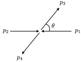
Figure 7: Kinematics of the $\,2\!\rightarrow\!2\,$ scattering process in the center-of-mass frame.

In the center-of-mass frame (Fig.7), we define the momenta as follows:

$$p_{1}^{\mu}= -\left(E,0,0,k\right), \quad\quad p_{2}^{\mu}=-\left(E,0,0,-k\right),$$

$$p_{3}^{\mu}= \left(E,ks_{\theta},0,kc_{\theta}\right), \quad\quad p_{4}^{\mu}=\left(E,-ks_{\theta},0,-kc_{\theta}\right),$$ (A.1)

where $k=|\vec{p}\,|$. Then, the Mandelstam variables $(s,t,u)$ take the following form:

$$s\, =-\left(p_{1}+p_{2}\right)^{2}=4E^{2}\,,$$ (A.2a)

$$t\, =-\left(p_{1}+p_{4}\right)^{2}=-\frac{s-4M_{n}^{2}}{2}(1+c_{\theta})\,,$$ (A.2b)

$$u\, =-\left(p_{1}+p_{3}\right)^{2}=-\frac{s-4M_{n}^{2}}{2}(1-c_{\theta})\,.$$ (A.2c)

Optionally, with Eq.(A.2), we can also use the relation $\,E^{2}\!=k^{2}\!+\!M_{n}^{2}\,$ to define another set of Mandelstam variables $(s_{0},t_{0},u_{0})$:

$$s_{0} \,=\,4k^{2}\,,$$ (A.3a)

$$t_{0} \,=\,-\frac{\,s_{0}\,}{2}(1+c_{\theta})\,,$$ (A.3b)

$$u_{0} \,=\,-\frac{\,s_{0}\,}{2}(1-c_{\theta})\,.$$ (A.3c)

The summations of the Mandelstam variables (A.2) and (A.3) obey the identities $\,s+t+u\!=\!4M_{n}^{2}$  and $\,s_{0}\!+t_{0}\!+u_{0}\!=0$ , respectively.

Moreover, the above formulas can be extended to the general scattering process $\,X_{n}X_{k}\!\!\rightarrow\!X_{m}X_{\ell}\,$,  where $\,n,k,m,\ell\!\geqslant 0$ . Thus, the sum of these Mandelstam variables $(s,t,u)$ satisfies $\,s+t+u=M_{n}^{2}\!+\!M_{k}^{2}\!+\!M_{m}^{2}\!+\!M_{\ell}^{2}$ . The incident and outgoing states have the following momenta in the center of mass frame,

$$p_{1}^{\mu}= -\!(E_{1},0,0,k), \hskip 28.45274ptp_{2}^{\mu}=-(E_{2},0,0,-k),$$

$$p_{3}^{\mu}= \,(E_{3},k^{\prime}s_{\theta},0,k^{\prime}c_{\theta}), \hskip 28.45274ptp_{4}^{\mu}=(E_{4},-k^{\prime}s_{\theta},0,-k^{\prime}c_{\theta}),$$ (A.4)

where the energy conservation condition, $\sqrt{s\,}\!=E_{1}\!+\!E_{2}=E_{3}\!+\!E_{4}$ ,  determines the momenta $k$ and $k^{\prime}$ as follows:

$$k =\frac{1}{\,2\sqrt{s\,}\,}\left([s-(M_{1}\!+\!M_{2})^{2}][s-(M_{1}\!-\!M_{2})^{2}]\right)^{\!{1}/{2}},$$

$$k^{\prime} =\frac{1}{\,2\sqrt{s\,}\,}\left([s-(M_{3}\!+\!M_{4})^{2}][s-(M_{3}\!-\!M_{4})^{2}]\right)^{\!{1}/{2}}.$$ (A.5)

Finally, as mentioned in section 2, a massive KK graviton has 5 helicity states ($\lambda\!=\pm 2,\pm 1,0$ ). Their polarization tensors take the following forms:

$$\varepsilon_{\pm 2}^{\mu\nu} =\epsilon_{\pm}^{\mu}\epsilon_{\pm}^{\nu}\,,\qquad\varepsilon_{\pm 1}^{\mu\nu}=\frac{1}{\sqrt{2\,}\,}\!\left(\epsilon_{\pm}^{\mu}\epsilon_{L}^{\nu}\!+\epsilon_{L}^{\mu}\epsilon_{\pm}^{\nu}\right)\!,\qquad\varepsilon_{L}^{\mu\nu}\!=\frac{1}{\sqrt{6\,}\,}\!\left(\epsilon_{+}^{\mu}\epsilon_{-}^{\nu}\!+\epsilon_{-}^{\mu}\epsilon_{+}^{\nu}\!+2\epsilon_{L}^{\mu}\epsilon_{L}^{\nu}\right)\!,$$ (A.6)

where $(\epsilon_{\pm}^{\mu},\,\epsilon_{L}^{\mu})$ denote the (transverse, longitudinal) polarization vectors of a vector boson with the same 4-momentum $p^{\mu}$. These polarization tensors satisfy the traceless and orthonormal conditions. They are also orthogonal to the 4-momentum $p^{\mu}$ of the KK graviton. Thus, the following conditions hold:

$$\eta_{\mu\nu}\varepsilon^{\mu\nu}=0\,,\qquad\varepsilon_{\lambda}^{\mu\nu}\varepsilon_{\lambda^{\prime}\!,\,\mu\nu}^{*}=\delta_{\lambda\lambda^{\prime}}\,,\qquad p_{\mu}\varepsilon^{\mu\nu}=0\,,$$ (A.7)

where $\,\lambda,\lambda^{\prime}\,(=\pm 2,\,\pm 1,\,0)\,$ are the helicity indices of the KK graviton.

Appendix B From $R_{\xi}$ Gauge to Unitary Gauge

We note that the KK graviton propagator (2.3ua) in the general $R_{\xi}$ gauge can be decomposed into the unitary gauge propagator (2.3w) plus the $\xi_{n}$-dependent part. In momentum space, we present this decomposition in the following form:

$$\mathcal{D}^{\mu\nu\alpha\beta}_{nm}(p)\ = \ \mathcal{D}_{nm,{\mathrm{UG}}}^{\mu\nu\alpha\beta}(p)+\mathcal{D}_{nm,\,\xi}^{\mu\nu\alpha\beta}(p)\,,$$ (B.1a)

$$\mathcal{D}_{nm,{\mathrm{UG}}}^{\mu\nu\alpha\beta}(p)\ = \ -\frac{\text{i}\delta_{nm}}{2}\frac{\leavevmode\nobreak\ \bar{\eta}^{\mu\alpha}\bar{\eta}^{\nu\beta}\!+\!\bar{\eta}^{\mu\beta}\bar{\eta}^{\nu\alpha}\!-\!\frac{2}{3}\bar{\eta}^{\mu\nu}\bar{\eta}^{\alpha\beta}\leavevmode\nobreak\ }{\,p^{2}\!+\!M_{n}^{2}\,}\,,$$ (B.1b)

$$\mathcal{D}_{nm,\,\xi}^{\mu\nu\alpha\beta}(p)\ = \ \frac{\text{i}\delta_{nm}/2}{\,p^{2}+\xi_{n}M_{n}^{2}\,}\biggl{[}\!\left(\!\eta^{\mu\alpha}\!+\!\frac{p^{\mu}p^{\alpha}}{\xi_{n}M_{n}^{2}\,}\!\right)\!\frac{p^{\nu}p^{\beta}}{\,\xi_{n}M_{n}^{2}\,}\!+\!\left(\!\eta^{\mu\beta}\!+\!\frac{p^{\mu}p^{\beta}}{\xi_{n}M_{n}^{2}\,}\!\right)\!\frac{p^{\nu}p^{\alpha}}{\,\xi_{n}M_{n}^{2}\,}$$

$$\ +\!\left(\!\eta^{\nu\alpha}\!+\!\frac{p^{\nu}p^{\alpha}}{\xi_{n}M_{n}^{2}\,}\!\right)\!\!\frac{p^{\mu}p^{\beta}}{\,\xi_{n}M_{n}^{2}\,}\!+\!\left(\!\eta^{\nu\beta}\!+\!\frac{p^{\nu}p^{\beta}}{\,\xi_{n}M_{n}^{2}\,}\!\right)\!\frac{p^{\mu}p^{\alpha}}{\,\xi_{n}M_{n}^{2}\,}\!\biggr{]}-\frac{\text{i}\delta_{nm}2p^{\mu}p^{\nu}p^{\alpha}p^{\beta}}{\,(p^{2}\!+\!\xi_{n}^{2}M_{n}^{2})\,\xi_{n}M_{n}^{4}\,}$$

$$\ +\frac{\text{i}\delta_{nm}/6}{\,p^{2}\!+\!(3\xi_{n}\!-\!2)M_{n}^{2}\,}\!\left(\!\eta^{\mu\nu}\!\!-\!\frac{\,2p^{\mu}p^{\nu}\,}{M_{n}^{2}}\!\right)\!\!\left(\!\eta^{\alpha\beta}\!-\!\frac{\,2p^{\alpha}p^{\beta}\,}{M_{n}^{2}}\!\right)\!,$$ (B.1c)

where $\,\bar{\eta}^{\mu\nu}\!=\!\eta^{\mu\nu}\!+p^{\mu}p^{\nu}\!/\!M^{2}$. We see that the $\xi_{n}$-dependent part $\mathcal{D}_{nm,\,\xi}^{\mu\nu\alpha\beta}(p)$ vanishes under $\,\xi_{n}\!\!\rightarrow\!\infty$. So, the propagator $\,\mathcal{D}^{\mu\nu\alpha\beta}_{nm}(p)\,$ will reduce to the unitary gauge form $\,\mathcal{D}_{nm,{\mathrm{UG}}}^{\mu\nu\alpha\beta}(p)\,$ in this limit. Also, the gravitational KK Goldstone propagators $\mathcal{D}_{nm}^{\mu\nu}(p)$ and $\mathcal{D}_{nm}(p)$ in Eqs.(2.3ub)-(2.3uc) vanish in this limit $\,\xi_{n}\!\!\rightarrow\!\infty\,$, which removes the unphysical KK Goldstone bosons in the unitary gauge as expected. For the Feynman-’t Hooft gauge ($\hskip 0.85358pt\xi_{n}\!=1$), we find that the $\xi_{n}$-dependent part of the KK graviton propagator takes a much simpler form:

$$\mathcal{D}_{nm,\,\xi}^{\mu\nu\alpha\beta}(p)\Big{|}_{\xi=1}= \ \frac{\text{i}\delta_{nm}/6}{\leavevmode\nobreak\ p^{2}\!+\!M_{n}^{2}\leavevmode\nobreak\ }\!\left(\!\eta^{\mu\nu}\!\!-\!\frac{\,2p^{\mu}p^{\nu}\,}{M_{n}^{2}}\!\right)\!\!\left(\!\eta^{\alpha\beta}\!-\!\frac{\,2p^{\alpha}p^{\beta}\,}{M_{n}^{2}}\!\right)$$

$$\ +\frac{\text{i}\delta_{nm}/2}{\,(p^{2}\!+\!M_{n}^{2})M_{n}^{2}\,}\!\left(p^{\mu}p^{\alpha}\eta^{\nu\beta}\!+p^{\nu}p^{\alpha}\eta^{\mu\beta}\!+p^{\mu}p^{\beta}\eta^{\nu\alpha}\!+p^{\nu}p^{\beta}\eta^{\mu\alpha}\right)\!.\hskip 28.45274pt$$ (B.2)

In passing, a $R_{\xi}$ gauge-fixing was considered [48] in the Randall-Sundrum model with warped 5d which contains additional terms related to warp parameter; we note that their KK graviton propagator was written in a rather different form, but can be converted into the form consistent with our (B.1).

We note that the Lagrangian (2.3m) is invariant under the general coordinate transformation (gauge transformation):

$$\hat{h}_{AB}\,\rightarrow\leavevmode\nobreak\ \hat{h}_{AB}^{\prime}=\hat{h}_{AB}-2\partial_{(A}\hat{\chi}_{B)}\,,$$ (B.3)

where $\hat{\chi}_{A}(x)$  is an infinitesimal translation which refers to a vector field generating a one-parameter diffeomorphism group in the background spacetime.

Taking Eq.(2.3h) under the KK expansion (2.3l), we derive the following gauge transformations for the KK fields:

$$h^{\mu\nu}_{n} \,\leavevmode\nobreak\ \rightarrow\leavevmode\nobreak\ \leavevmode\nobreak\ h^{\prime\,\mu\nu}_{n}=\,h^{\mu\nu}_{n}-2\partial^{(\mu}\chi^{\nu)}_{n}-M_{n}\eta^{\mu\nu}\chi^{5}_{n}\,,$$ (B.4a)

$$\mathcal{A}^{\mu}_{n} \,\leavevmode\nobreak\ \rightarrow\leavevmode\nobreak\ \leavevmode\nobreak\ \mathcal{A}^{\prime\,\mu}_{n}=\,\mathcal{A}^{\mu}_{n}-\partial^{\mu}\chi^{5}_{n}+M_{n}\chi^{\mu}_{n}\,,$$ (B.4b)

$$\phi_{n} \,\leavevmode\nobreak\ \rightarrow\leavevmode\nobreak\ \leavevmode\nobreak\ \phi^{\prime}_{n}=\,\phi_{n}-2M_{n}\chi^{5}_{n}\,.$$ (B.4c)

In the above the group parameters $(\chi_{n}^{\mu},\,\chi_{n}^{5})$ arise from the following KK expansions of the corresponding 5d parameters $(\hat{\chi}^{\mu},\,\hat{\chi}^{5})$:

$$\hat{\chi}^{\mu}(x^{\nu},x^{5}) \,=\,\frac{1}{\sqrt{L}}\left[\,\chi^{\mu}_{0}(x^{\nu})+\sqrt{2}\sum_{n=1}^{\infty}\chi^{\mu}_{n}(x^{\nu})\cos\!\frac{\,n\pi x^{5}\,}{L}\,\right]\!,$$ (B.5a)

$$\hat{\chi}^{5}(x^{\nu},x^{5}) \,=\,\sqrt{\frac{2}{L}}\,\sum_{n=1}^{\infty}\chi^{5}_{n}(x^{\nu})\sin\!\frac{\,n\pi x^{5}\,}{L}\,,$$ (B.5b)

where we set $\,(\hat{\chi}^{\mu},\,\hat{\chi}^{5})$  as  (even, odd)  under the $\mathbb{Z}_{2}$ reflection of 5d orbifold.

To transform into unitary gauge, we choose the gauge parameters as follows:

$$\chi^{\mu}_{n}=-\frac{1}{M_{n}}\!\left(\!\mathcal{A}^{\mu}_{n}-\frac{\,\partial^{\mu}\phi_{n}\,}{2M_{n}}\right)\!,\quad\leavevmode\nobreak\ \leavevmode\nobreak\ \leavevmode\nobreak\ \chi^{5}_{n}=\frac{\phi_{n}}{2M_{n}}\,.$$ (B.6)

Then, we derive the field transformations to the unitary gauge:

$$h^{\mu\nu}_{n} \,\leavevmode\nobreak\ \rightarrow\leavevmode\nobreak\ \leavevmode\nobreak\ h^{\prime\,\mu\nu}_{n}\!=\,h^{\mu\nu}_{n}+\frac{2}{M_{n}}\,\partial^{(\mu}\!\mathcal{A}^{\nu)}_{n}-\frac{1}{2}\!\left(\!\eta^{\mu\nu}\!+\!\frac{2\partial^{\mu}\partial^{\nu}}{M_{n}^{2}}\right)\!\phi_{n}\,,$$ (B.7a)

$$\mathcal{A}^{\mu}_{n} \,\leavevmode\nobreak\ \rightarrow\leavevmode\nobreak\ \leavevmode\nobreak\ \mathcal{A}^{\prime\,\mu}_{n}=\,0\,,$$ (B.7b)

$$\phi_{n} \,\leavevmode\nobreak\ \rightarrow\leavevmode\nobreak\ \leavevmode\nobreak\ \phi_{n}^{\prime}=\,0\,.$$ (B.7c)

Thus, under the unitary gauge, both the KK Goldstone states $\,\mathcal{A}^{\mu}_{n}\,$ and $\,\phi_{n}$ ($n\!>\!0$) are gauged away, so the 4d action of the Lagrangian (2.2) becomes:

$$S_{\mathrm{eff}} \,=\int\!\text{d}^{4}x\!\sum_{n=0}^{\infty}\bigg{\{}\!\!-\mbox{$\frac{\,{1}\,}{2}$}(\partial^{\mu}h_{n})^{2}+\mbox{$\frac{\,{1}\,}{2}$}(\partial^{\rho}h_{n}^{\mu\nu})^{2}+\partial_{\mu}h^{\mu\nu}_{n}\partial_{\nu}h_{n}-\partial_{\mu}h^{\mu\rho}_{n}\partial^{\nu}h_{\nu\rho,n}$$

$$\hskip 60.00009pt-\mbox{$\frac{\,{1}\,}{2}$}M^{2}_{n}\left[\,h_{n}^{2}\!-\!(h^{\mu\nu}_{n})^{2}\,\,\right]\!\bigg{\}}+\mbox{$\frac{\,{3}\,}{4}$}(\partial_{\mu}\phi_{0})^{2}\,.$$ (B.8)

Appendix C Feynman Rules for KK Graviton Interaction with Matter

In this Appendix, we present the relevant Feynman rules of the 5d gravitational scalar QED (GSQED5) as studied in section 4.1, including the propagators of the matter fields and the vertices for the KK graviton (Goldstone) interaction with the matter fields. All the Feynman Rules are derived in the Feynman-’t Hooft gauge ($\zeta_{n}=1$).

We first present the photon propagator and scalar propagator as follows:

$$\mathcal{D}_{nm}^{\mu\nu}(p)=\frac{-\text{i}\eta^{\mu\nu}\delta_{nm}}{p^{2}+M_{n}^{2}}\,,\qquad\mathcal{D}_{nm}(p)=\frac{\text{i}\delta_{nm}}{p^{2}+m_{n}^{2}}\,,$$ (C.1)

where the KK number  $n\!\geqslant\!0$  and the KK mass for the scalar field is $\,m_{n}\!=\!\sqrt{m_{0}^{2}\!+\!M_{n}^{2}\,}\,$.

Then, with the relations between the 4d coupling constants and 5d couplings $\,e=\hat{e}/\!\sqrt{L\,}$  and $\,\kappa=\hat{\kappa}/\!\sqrt{L\,}$ ,  we derive the cubic and quartic interaction vertices for the KK graviton (Goldstone) interactions with matter, which are presented in Fig. 8.

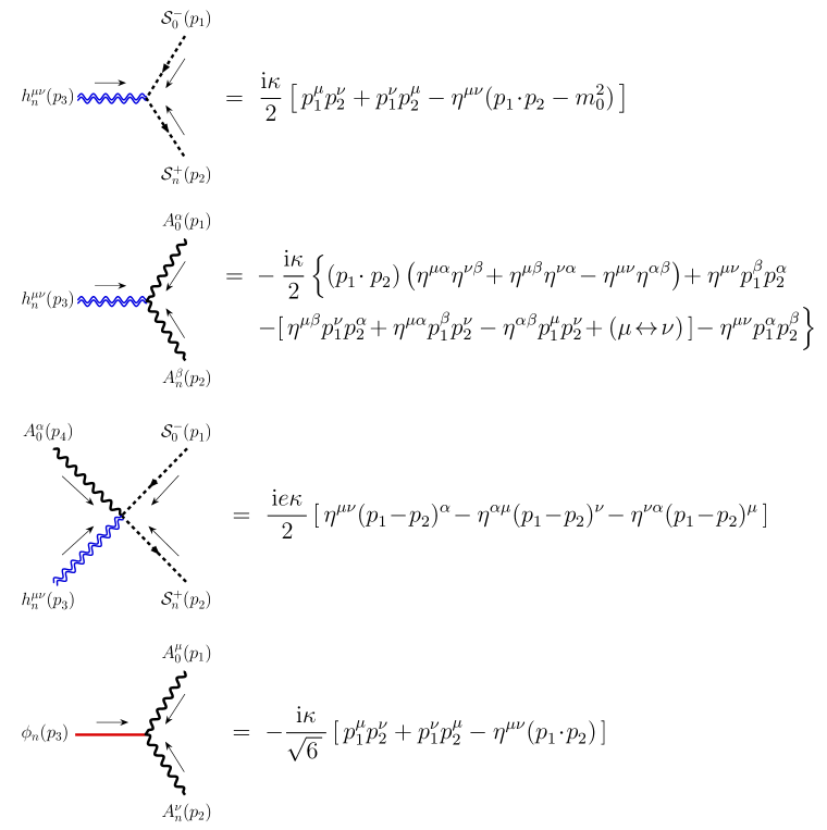
Figure 8: Feynman rules for the cubic and quartic interaction vertices between the KK graviton (KK Goldstone boson) and matter fields.

Appendix D Gravitational KK Goldstone Amplitudes from Goldstone Exchanges and Contact Interactions

In this Appendix, we derive the Feynman rules of the KK Goldstone self-interactions which we will use to compute the subleading diagrams in Fig. 5, for the analysis of section 4.2.

$\hat{\mathcal{L}}_{1}[\hat{\mathcal{A}}\hat{\phi}^{2}]$	$\hat{\mathcal{A}}^{\mu}\partial_{\mu}\hat{\phi}\,\partial_{5}\hat{\phi}$	$\hat{\mathcal{A}}^{\mu}(\partial_{\mu}\partial_{5}\hat{\phi})\hat{\phi}$	$\partial_{\mu}\hat{\mathcal{A}}^{\mu}\partial_{5}\hat{\phi}\,\hat{\phi}$	$\partial_{5}\hat{\mathcal{A}}^{\mu}\partial_{\mu}\hat{\phi}\,\hat{\phi}$	$\partial_{\mu}\partial_{5}\hat{\mathcal{A}}^{\mu}\hat{\phi}^{2}$
$\hat{\mathcal{L}}_{1}[\hat{\phi}^{3}]$	$\hat{\phi}(\partial_{\mu}\hat{\phi})^{2}$	$\hat{\phi}(\partial_{5}\hat{\phi})^{2}$	$\hat{\phi}^{2}\partial_{\mu}^{2}\hat{\phi}$	$\hat{\phi}^{2}\partial_{5}^{2}\hat{\phi}$
$\hat{\mathcal{L}}_{2}[\hat{\phi}^{4}]$	$\hat{\phi}^{2}(\partial_{\mu}\hat{\phi})^{2}$	$\hat{\phi}^{2}(\partial_{5}\hat{\phi})^{2}$	$\hat{\phi}^{3}\partial_{\mu}^{2}\hat{\phi}$	$\hat{\phi}^{3}\partial_{5}^{2}\hat{\phi}$

Table 2: Lorentz-invariant vertices in the 5d Lagrangian terms $\hat{\mathcal{L}}_{1}[\hat{\mathcal{A}}\hat{\phi}^{2}]$,  $\hat{\mathcal{L}}_{1}[\hat{\phi}^{3}]$, and $\,\hat{\mathcal{L}}_{2}[\hat{\phi}^{4}]$.

Under the basis defined in Table 2, we can expand the Lorentz-invariant structure of 5d Lagrangian terms $\hat{\mathcal{L}}_{1}[\hat{\mathcal{A}}\hat{\phi}^{2}]$,  $\hat{\mathcal{L}}_{1}[\hat{\phi}^{3}]$,  and $\hat{\mathcal{L}}_{2}[\hat{\phi}^{4}]$ as follows:

$$\hat{\mathcal{L}}_{1}[\hat{\mathcal{A}}\hat{\phi}^{2}] \,=\,b_{1}\,\hat{\mathcal{A}}^{\mu}\partial_{\mu}\hat{\phi}\,\partial_{5}\hat{\phi}+b_{2}\,\hat{\mathcal{A}}^{\mu}\hat{\phi}\,\partial_{\mu}\partial_{5}\hat{\phi}\,,$$ (D.4a)

$$\hat{\mathcal{L}}_{1}[\hat{\phi}^{3}] \,=\,c_{1}\,\hat{\phi}\,(\partial_{\mu}\hat{\phi})^{2}+c_{2}\,\hat{\phi}\,(\partial_{5}\hat{\phi})^{2}\,,$$ (D.4b)

$$\hat{\mathcal{L}}_{2}[\hat{\phi}^{4}] \,=\,d_{1}\,\hat{\phi}^{2}(\partial_{\mu}\hat{\phi})^{2}+d_{2}\,\hat{\phi}^{2}(\partial_{5}\hat{\phi})^{2}\,,$$ (D.4c)

where we have computed systematically the coefficients $(b_{1},\,b_{2},\,c_{1},\,c_{2},\,d_{1},\,d_{2})$ as follows:

$$(b_{1},\,b_{2},\,c_{1},\,c_{2},\,d_{1},\,d_{2})\,=\left(0,\,\frac{1}{\sqrt{2\,}\,},\,\sqrt{\frac{2}{3}\,},\,-\frac{1}{\sqrt{6\,}\,}\,,-\frac{1}{\,8\,},\,\frac{1}{\,4\,}\right)\!.$$ (D.5)

Then, by integrating over $x^{5}$ on the 5d interval $[0,\,L]$, we derive the 4d effective KK Lagrangian terms as follows:

$$\mathcal{L}_{1}[\mathcal{A}\phi^{2}] =-\frac{\kappa}{\sqrt{2\,}}\sum_{n,m,\ell=1}^{\infty}\!\biggl{\{}b_{1}M_{\ell}[\sqrt{2}\mathcal{A}^{\mu}_{n}\partial_{\mu}\phi_{0}\phi_{\ell}\delta_{n\ell}+\mathcal{A}^{\mu}_{n}\partial_{\mu}\phi_{m}\phi_{\ell}\widetilde{\Delta}_{3}(m,n,\ell)]$$

$$+b_{2}M_{\ell}[\sqrt{2}\mathcal{A}^{\mu}_{n}\phi_{0}\partial_{\mu}\phi_{\ell}\delta_{n\ell}+\mathcal{A}^{\mu}_{n}\phi_{m}\partial_{\mu}\phi_{\ell}\widetilde{\Delta}_{3}(m,n,\ell)]\biggr{\}},$$ (D.6a)

$$\mathcal{L}_{1}[\phi^{3}] =\frac{\kappa}{\sqrt{2\,}}\sum_{n,m,\ell=1}^{\infty}\bigg{\{}c_{1}[\sqrt{2}(\phi_{0}(\partial_{\mu}\phi_{0})^{2}+\phi_{0}\partial_{\mu}\phi_{m}\partial^{\mu}\phi_{\ell}\,\delta_{m\ell}+\phi_{n}\partial_{\mu}\phi_{0}\partial^{\mu}\phi_{m}\delta_{nm}$$

$$+\phi_{n}\partial_{\mu}\phi_{0}\partial^{\mu}\phi_{\ell}\,\delta_{n\ell})+\phi_{n}\partial_{\mu}\phi_{m}\partial^{\mu}\phi_{\ell}\Delta_{3}(n,m,\ell)]+c_{2}M_{m}M_{\ell}[\sqrt{2}\,\phi_{0}\phi_{m}\phi_{\ell}\delta_{m\ell}$$

$$+\phi_{n}\phi_{m}\phi_{\ell}\widetilde{\Delta}_{3}(n,m,\ell)]\bigg{\}},$$ (D.6b)

$$\mathcal{L}_{2}[\phi^{4}] =\frac{\kappa^{2}}{2\,}\!\sum_{n,m,\ell,k=1}^{\infty}\biggl{\{}d_{1}\{2\left(\phi_{0}\partial_{\mu}\phi_{0}\right)^{2}+2[\left(\partial_{\mu}\phi_{0}\right)^{2}\phi_{n}\phi_{m}\delta_{nm}+\phi_{0}\partial_{\mu}\phi_{0}\phi_{n}\partial^{\mu}\phi_{\ell}\delta_{n\ell}$$

$$+\phi_{0}\partial_{\mu}\phi_{0}\phi_{n}\partial^{\mu}\phi_{k}\delta_{nk}+\phi_{0}\partial_{\mu}\phi_{0}\phi_{m}\partial^{\mu}\phi_{k}\delta_{mk}+\phi_{0}\partial_{\mu}\phi_{0}\phi_{m}\partial^{\mu}\phi_{\ell}\delta_{m\ell}+\phi_{0}^{2}\partial_{\mu}\phi_{\ell}\partial^{\mu}\phi_{k}\delta_{\ell k}]$$

$$+\sqrt{2}[\partial_{\mu}\phi_{0}\phi_{n}\phi_{m}\partial^{\mu}\phi_{\ell}\Delta_{3}(n,m,\ell)+\partial_{\mu}\phi_{0}\phi_{n}\phi_{m}\partial^{\mu}\phi_{k}\Delta_{3}(n,m,k)+\partial_{\mu}\phi_{0}\phi_{n}\phi_{\ell}\partial^{\mu}\phi_{k}\Delta_{3}(n,\ell,k)$$

$$+\phi_{0}\phi_{m}\partial_{\mu}\phi_{\ell}\partial^{\mu}\phi_{k}\Delta_{3}(m,\ell,k)]+\phi_{n}\phi_{m}\partial_{\mu}\phi_{\ell}\partial^{\mu}\phi_{k}\Delta_{4}(n,m,\ell,k)\}+d_{2}M_{\ell}M_{k}[2(\phi_{0})^{2}\phi_{\ell}\phi_{k}\delta_{\ell k}$$

$$+\sqrt{2}\phi_{0}\phi_{m}\phi_{\ell}\phi_{k}\widetilde{\Delta}_{3}(m,\ell,k)+\sqrt{2}\phi_{0}\phi_{n}\phi_{\ell}\phi_{k}\widetilde{\Delta}_{3}(n,\ell,k)+\phi_{n}\phi_{m}\phi_{\ell}\phi_{k}\widetilde{\Delta}_{4}(n,m,\ell,k)]\biggr{\}},$$ (D.6c)

where

$$\Delta_{4}(n,m,\ell,k)= \,\,\delta(n\!+\!m\!+\!\ell\!-\!k)+\delta(n\!+\!m\!-\!\ell\!-\!k)+\delta(n\!-\!m\!+\!\ell\!-\!k)+\delta(n\!-\!m\!-\!\ell\!-\!k)\hskip 36.98857pt$$

$$+\delta(n\!-\!m\!-\!\ell\!+\!k)+\delta(n\!+\!m\!-\!\ell\!+\!k)+\delta(n\!-\!m\!+\!\ell\!+\!k)\,,$$ (D.7a)

$$\widetilde{\Delta}_{4}(n,m,\ell,k)= \,\,\delta(n\!+\!m\!+\!\ell\!-\!k)-\delta(n\!+\!m\!-\!\ell\!-\!k)+\delta(n\!-\!m\!+\!\ell\!-\!k)-\delta(n\!-\!m\!-\!\ell\!-\!k)$$

$$+\delta(n\!-\!m\!-\!\ell\!+\!k)-\delta(n\!+\!m\!-\!\ell\!+\!k)+\delta(n\!-\!m\!+\!\ell\!+\!k)\,.$$ (D.7b)

With these, we derive the cubic and quartic interaction vertices of $\mathcal{A}\phi^{2}$, $\phi^{3}$, and $\phi^{4}$, which are presented in Fig. 9.

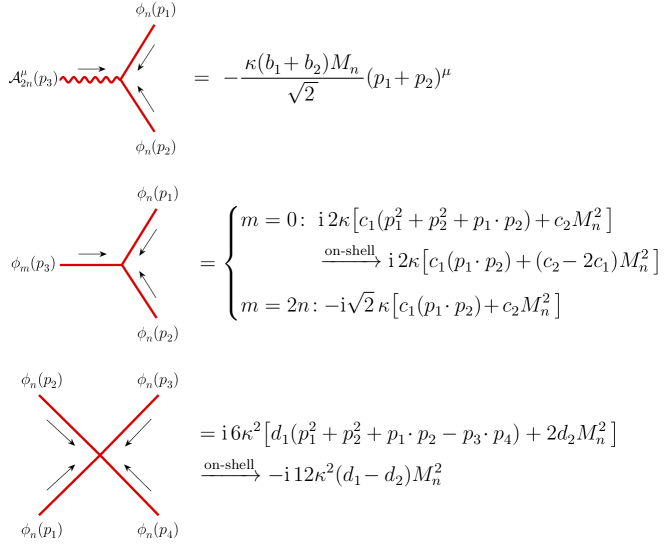
Figure 9: Feynman rules for the cubic and quartic interaction vertices among the KK gravitational Goldstone bosons $\phi_{n}$ and $\mathcal{A}^{\mu}_{n}$ .

By explicit calculations, we find that the scattering amplitudes of $\,\phi_{n}\phi_{n}\!\!\rightarrow\!\phi_{n}\phi_{n}\,$ from the $\phi_{0}$ ($\phi_{2n}$) exchanges and from the contact interaction are all of $\,\mathcal{O}(M_{n}^{2})\,$ under the high energy expansion, which do not contribute to the LO Goldstone boson amplitude of $\mathcal{O}(E^{2})$ . This conclusion still holds for the inelastic scattering process $\phi_{n}\phi_{k}\!\rightarrow\!\phi_{m}\phi_{\ell}$ .

Appendix E Massless Graviton Scattering and Double-Copy in 4d

For the sake of comparison, in this Appendix we compute the scattering amplitudes of four gluons and of four gravitons at tree level in 4d, by using the conventional Feynman techniques and the reduced super-string amplitudes, respectively. We also verify the double-copy construction of massless graviton amplitudes from the massless gluon amplitudes by using the color-kinematics (CK) duality. We find that the conversion constant between the gauge boson coupling and the graviton coupling in 4d differs from what we have obtained in the 5d KK theory analysis (section 5.2).

Massless Graviton Scattering from Double-Copy Construction in 4d

For an SU(N) non-Abelian gauge theory, we can express the four-gluon scattering amplitudes at tree level as follows:

$$\mathcal{T}[gg\rightarrow gg]\,=\,-g^{2}\,(\mathcal{T}_{c}+\mathcal{T}_{s}+\mathcal{T}_{t}+\mathcal{T}_{u})\,,$$ (E.1)

where the amplitude contains the contributions from a contact interaction diagram and the $(s,t,u)$-channel pole-diagrams whose amplitudes are given by

$$\mathcal{T}_{c}\ = \ \ \mathcal{C}_{s}\left[\,(\epsilon_{1}\!\cdot\epsilon_{3})(\epsilon_{2}\!\cdot\epsilon_{4})-(\epsilon_{1}\!\cdot\epsilon_{4})(\epsilon_{2}\!\cdot\epsilon_{3})\,\right]+\mathcal{C}_{t}\left[\,(\epsilon_{1}\!\cdot\epsilon_{2})(\epsilon_{3}\!\cdot\epsilon_{4})-(\epsilon_{1}\!\cdot\epsilon_{3})(\epsilon_{2}\!\cdot\epsilon_{4})\,\right]\hskip 22.76219pt$$

$$\ +\mathcal{C}_{u}\left[\,(\epsilon_{1}\!\cdot\epsilon_{4})(\epsilon_{2}\!\cdot\epsilon_{3})-(\epsilon_{1}\!\cdot\epsilon_{2})(\epsilon_{3}\!\cdot\epsilon_{4})\,\right],$$ (E.2a)

$$\mathcal{T}_{s}\ = \ \ \frac{\,\mathcal{C}_{s}\,}{s}\left[\,\left(p_{1}\!-p_{2}\right)(\epsilon_{1}\!\cdot\epsilon_{2})+2(p_{2}\!\cdot\epsilon_{1})\epsilon_{2}-2(p_{1}\!\cdot\epsilon_{2})\epsilon_{1}\,\right]$$

$$\hskip 20.00003pt\cdot\left[\,\left(p_{4}\!-p_{3}\right)(\epsilon_{3}\!\cdot\epsilon_{4})+2(p_{3}\!\cdot\epsilon_{4})\epsilon_{3}-2(p_{4}\!\cdot\epsilon_{3})\epsilon_{4}\,\right],$$ (E.2b)

$$\mathcal{T}_{t}\ = \ \ -\frac{\leavevmode\nobreak\ \mathcal{C}_{t}\,}{t}\left[\,\left(-p_{1}\!+p_{4}\right)(\epsilon_{1}\!\cdot\epsilon_{4})-2(p_{4}\!\cdot\epsilon_{1})\epsilon_{4}+2(p_{1}\!\cdot\epsilon_{4})\epsilon_{1}\,\right]$$

$$\hskip 20.00003pt\cdot\left[\,\left(-p_{2}\!+p_{3}\right)(\epsilon_{2}\!\cdot\epsilon_{3})-2(p_{3}\!\cdot\epsilon_{2})\epsilon_{3}+2(p_{2}\!\cdot\epsilon_{3})\epsilon_{2}\,\right],$$ (E.2c)

$$\mathcal{T}_{u}\ = \ \ \frac{\leavevmode\nobreak\ \mathcal{C}_{u}\,}{u}\left[\,\left(-p_{1}\!+p_{3}\right)(\epsilon_{1}\!\cdot\epsilon_{3})-2(p_{3}\!\cdot\epsilon_{1})\epsilon_{3}+2(p_{1}\!\cdot\epsilon_{3})\epsilon_{1}\,\right]$$

$$\hskip 20.00003pt\cdot\left[\,\left(-p_{2}\!+p_{4}\right)(\epsilon_{2}\!\cdot\epsilon_{4})-2(p_{4}\!\cdot\epsilon_{2})\epsilon_{4}+2(p_{2}\!\cdot\epsilon_{4})\epsilon_{2}\,\right].$$ (E.2d)

Here each external massless gauge boson (gluon) has two helicity states, as described by its two transverse polarization vectors $\,\epsilon_{j\pm}^{\mu}\,$ ($j=1,2,3,4$):

$$\epsilon^{\mu}_{1+}=\epsilon^{\mu}_{2-} =\frac{1}{\sqrt{2\,}\,}(0,1,\text{i},0), \qquad\epsilon^{\mu}_{1-}=\epsilon^{\mu}_{2+}=\frac{1}{\sqrt{2\,}\,}(0,-1,\text{i},0),$$

$$\epsilon^{\mu}_{3+}=\epsilon^{\mu}_{4-} =\frac{1}{\sqrt{2\,}\,}(0,\text{i}c_{\theta},1,-\text{i}s_{\theta}), \qquad\epsilon^{\mu}_{3-}=\epsilon^{\mu}_{4+}=\frac{1}{\sqrt{2\,}\,}(0,\text{i}c_{\theta},-1,-\text{i}s_{\theta}).$$ (E.3)

Then, we compute the helicity amplitudes of the gauge boson scattering:

$$\mathcal{T}[++++]=\mathcal{T}[----]$$

$$\hskip 58.32823pt=g^{2}\!\left\{\mathcal{C}_{s}\left(-2c_{\theta}\right)+\mathcal{C}_{t}\left[\,\!\frac{3-2c_{\theta}-c_{2\theta}}{1-c_{\theta}}\!\,\right]+\mathcal{C}_{u}\left[\,\!\frac{-3-2c_{\theta}+c_{2\theta}}{1+c_{\theta}}\!\,\right]\right\}\!,$$ (E.4a)

$$\mathcal{T}[+-+-]=\mathcal{T}[-+-+]$$

$$\hskip 58.32823pt=g^{2}\!\left\{\mathcal{C}_{t}\left(-1-c_{\theta}\right)+\mathcal{C}_{u}\left[\,\!\frac{3+4c_{\theta}+c_{2\theta}}{2(1-c_{\theta})}\!\,\right]\right\}\!,$$ (E.4b)

$$\mathcal{T}[+--+]=\mathcal{T}[-++-]$$

$$\hskip 58.32823pt=g^{2}\!\left\{\mathcal{C}_{t}\left[\,\!\frac{-3+4c_{\theta}-c_{2\theta}}{2(1+c_{\theta})}\!\,\right]+\mathcal{C}_{u}\left(1-c_{\theta}\right)\right\},$$ (E.4c)

where $\,c_{2\theta}\!=\!\cos 2\theta$,  and all the helicity-flipped amplitudes vanish, which include the amplitudes like $\mathcal{T}[+++-]$, $\mathcal{T}[++--]$, and so on. For convenience, we rewrite the above amplitudes (E.4)-(E.4) as follows:

$$\mathcal{T}[++++]\,=\,\mathcal{T}[----] \,=\,g^{2}\!\left[\,\!\frac{\mathcal{C}_{s}\mathcal{N}_{s}}{s}+\frac{\mathcal{C}_{t}\mathcal{N}_{t}}{t}+\frac{\mathcal{C}_{u}\mathcal{N}_{u}}{u}\!\,\right]\!,$$ (E.5a)

$$\mathcal{T}[+-+-]\,=\,\mathcal{T}[-+-+] \,=\,g^{2}\!\left[\,\!\frac{\mathcal{C}_{s}\mathcal{N}^{\prime}_{s}}{s}+\frac{\mathcal{C}_{t}\mathcal{N}^{\prime}_{t}}{t}+\frac{\mathcal{C}_{u}\mathcal{N}^{\prime}_{u}}{u}\!\,\right]\!,$$ (E.5b)

$$\mathcal{T}[+--+]\,=\,\mathcal{T}[-++-] \,=\,g^{2}\!\left[\,\!\frac{\mathcal{C}_{s}\mathcal{N}^{\prime\prime}_{s}}{s}+\frac{\mathcal{C}_{t}\mathcal{N}^{\prime\prime}_{t}}{t}+\frac{\mathcal{C}_{u}\mathcal{N}^{\prime\prime}_{u}}{u}\!\,\right]\!,$$ (E.5c)

where the numerator parameters $(\mathcal{N}_{j},\,\mathcal{N}_{j}^{\prime},\,\mathcal{N}_{j}^{\prime\prime})$ are given by

$$\mathcal{N}_{s} =-2sc_{\theta}\,,\hskip 14.22636pt\mathcal{N}_{t} =\frac{\,s\,}{2}(-3+\!2c_{\theta}\!+c_{2\theta})\,,\hskip 14.22636pt\hskip 19.91692pt\mathcal{N}_{u} =\frac{\,s\,}{2}(3+\!2c_{\theta}\!-c_{2\theta})\,,$$ (E.6a)

$$\mathcal{N}^{\prime}_{s} =0\,,\qquad\hskip 14.22636pt\mathcal{N}^{\prime}_{t} =\frac{\,s(2\!+\!c_{\theta}\!-2c_{2\theta}\!-c_{3\theta})\,}{8(1\!-\!c_{\theta})}\,,\hskip 14.22636pt\hskip 3.69885pt\mathcal{N}^{\prime}_{u} =\frac{\,s(-2\!-c_{\theta}\!+2c_{2\theta}\!+\!c_{3\theta})\,}{8(1\!-\!c_{\theta})}\,,$$ (E.6b)

$$\mathcal{N}^{\prime\prime}_{s} =0\,,\qquad\hskip 14.22636pt\mathcal{N}^{\prime\prime}_{t} =\frac{\,s(2\!-\!c_{\theta}\!-\!2c_{2\theta}\!+\!c_{3\theta})\,}{8(1\!+\!c_{\theta})}\,,\hskip 14.22636pt\hskip 3.69885pt\mathcal{N}^{\prime\prime}_{u} =\frac{\,s(-2\!+\!c_{\theta}\!+\!2c_{2\theta}\!-\!c_{3\theta})\,}{8(1\!+\!c_{\theta})}\,.$$ (E.6c)

Hence, we can readily verify that the numerators in Eq.(E.6) obey the kinematic Jacobi identity:

$$\mathcal{N}_{s}+\mathcal{N}_{t}+\mathcal{N}_{u} \,=\,0\,,$$ (E.7a)

$$\mathcal{N}^{\prime}_{s}+\mathcal{N}^{\prime}_{t}+\mathcal{N}^{\prime}_{u} \,=\,0\,,$$ (E.7b)

$$\mathcal{N}^{\prime\prime}_{s}+\mathcal{N}^{\prime\prime}_{t}+\mathcal{N}^{\prime\prime}_{u} \,=\,0\,.$$ (E.7c)

Next, by using the double-copy approach with CK duality, we reconstruct the massless graviton scattering amplitudes as follows:

$$\mathcal{T}_{\mathrm{DC}}[++++]\,=\,\mathcal{T}_{\mathrm{DC}}[----] \,=\,-16\tilde{c}_{0}g^{2}s\csc^{2}\!\theta =\,-\frac{\kappa^{2}}{4}\frac{s^{3}}{\,t\hskip 1.3ptu\,}\,,$$ (E.8a)

$$\mathcal{T}_{\mathrm{DC}}[+-+-]\,=\,\mathcal{T}_{\mathrm{DC}}[-+-+] \,=\,-\,\tilde{c}_{0}g^{2}\frac{s\,s^{6}_{\theta}}{\,(1\!-\!c_{\theta})^{4}\,} =\,-\frac{\kappa^{2}}{4}\frac{t^{3}}{\,s\hskip 1.3ptu\,}\,,$$ (E.8b)

$$\mathcal{T}_{\mathrm{DC}}[+--+]\,=\,\mathcal{T}_{\mathrm{DC}}[-++-] \,=\,-\,\tilde{c}_{0}g^{2}\frac{s\left(1-c_{\theta}\right)^{4}}{s^{2}_{\theta}} =\,-\frac{\kappa^{2}}{4}\frac{u^{3}}{\,s\hskip 1.3ptt\,}\,,$$ (E.8c)

where we have applied the conversion constant (2.3an) for the amplitudes in the last equality of Eqs.(E.8a)-(E.8c) and $(+,-)\equiv(+2,-2)$. The above reconstructed massless graviton scattering amplitudes agree with the results of Refs. [49][50] which computed directly the graviton amplitudes by the conventional Feynman techniques.

Massless Graviton Scattering from Type-II Superstring Theory

The massless graviton scattering amplitudes can be computed by the conventional Feynman technique in quantum field theory. The 3-point and 4-point graviton interaction vertices were derived by DeWitt [51]. It is clear that by using the conventional Feynman diagram approach, the calculations of graviton scattering amplitudes are extremely complicated and tedious. Hence, we will use the amplitudes as computed within the type-II superstring theory (SST-II) [2][52][53]. The massless gravitons are described by closed strings and their 4-point scattering amplitude at tree level in the SST-II is given by

$$\mathcal{M}[\lambda_{1}\lambda_{2}\lambda_{3}\lambda_{4}]\,=\,\hat{\kappa}^{2}C(\hat{s},\hat{t},\hat{u})\,\varepsilon_{\lambda_{1}}^{\hat{\mu}\hat{\alpha}}\varepsilon_{\lambda_{2}}^{\hat{\nu}\hat{\beta}}\varepsilon_{\lambda_{3}}^{\hat{\rho}\hat{\gamma}}\varepsilon_{\lambda_{4}}^{\hat{\sigma}\hat{\lambda}}\widehat{K}_{\hat{\mu}\hat{\nu}\hat{\rho}\hat{\sigma}}\widehat{K}_{\hat{\alpha}\hat{\beta}\hat{\gamma}\hat{\lambda}}\,,$$ (E.9)

where $\,\hat{\kappa}\,$ is the 10-dimensional gravitational coupling constant, and the Mandelstam variables $(\hat{s},\,\hat{t},\,\hat{u})$ and the Lorentz indices $(\hat{\mu},\hat{\nu},\cdots)$ are defined in 10d. In Eq.(E.9), the $C$ function takes the following form:

$$C(\hat{s},\hat{t},\hat{u})\,=\,\frac{1}{\,128\,}\frac{\leavevmode\nobreak\ \Gamma(-\alpha^{\prime}\hat{s}/2)\Gamma(-\alpha^{\prime}\hat{t}/2)\Gamma(-\alpha^{\prime}\hat{u}/2)\leavevmode\nobreak\ }{\,\Gamma(1\!+\!\alpha^{\prime}\hat{s}/2)\Gamma(1\!+\!\alpha^{\prime}\hat{t}/2)\Gamma(1\!+\!\alpha^{\prime}\hat{u}/2)\,}\,,$$ (E.10)

where we have set the Regge slope for the closed string to be $\,\alpha^{\prime}\!=\!\mbox{$\frac{\,{1}\,}{4}$}\,$.

Using the relation of gamma functions $\,\Gamma(1\!+\!z)\!=\!z\Gamma(z)\,$, we can rewrite the function $C(\hat{s},\hat{t},\hat{u})$  as follows:

$$C(\hat{s},\hat{t},\hat{u})\,=\,-\frac{4}{\,\hat{s}\,\hat{t}\,\hat{u}\,}\frac{\leavevmode\nobreak\ \Gamma(1\!-\!\alpha^{\prime}\hat{s}/2)\,\Gamma(1\!-\!\alpha^{\prime}\hat{t}/2)\,\Gamma(1\!-\!\alpha^{\prime}\hat{u}/2)\leavevmode\nobreak\ }{\leavevmode\nobreak\ \Gamma(1\!+\!\alpha^{\prime}\hat{s}/2)\,\Gamma(1\!+\!\alpha^{\prime}\hat{t}/2)\,\Gamma(1\!+\!\alpha^{\prime}\hat{u}/2)\,}\,.$$ (E.11)

With Ref. [52], we note that by imposing compactification of  $(10\!-\!d)$  spatial dimensions, the amplitude defined in $d$-dimension has the same structure as that of the original 10-dimension case at tree level. In order to reduce the SST-II amplitude (E.9) to the amplitude in 4d , we take the limit for Regge slope $\,\alpha^{\prime}\!\rightarrow\!0$  and derive the reduced 4d graviton scattering amplitude:

$$\mathcal{M}[\lambda_{1}\lambda_{2}\lambda_{3}\lambda_{4}]\,=\,-\frac{\,4\kappa^{2}\,}{\,s\hskip 1.2ptt\hskip 1.0ptu\,}K_{\lambda_{1}^{\prime}\lambda_{2}^{\prime}\lambda_{3}^{\prime}\lambda_{4}^{\prime}}^{2},$$ (E.12)

where the $K_{\lambda_{1}^{\prime}\lambda_{2}^{\prime}\lambda_{3}^{\prime}\lambda_{4}^{\prime}}$ factor is given as follows [2][52][53]:

$$K_{\lambda_{1}^{\prime}\lambda_{2}^{\prime}\lambda_{3}^{\prime}\lambda_{4}^{\prime}}\!= -\frac{1}{4}\big{\{}[st(\epsilon_{1}\!\cdot\epsilon_{3})(\epsilon_{2}\!\cdot\epsilon_{4})+su(\epsilon_{1}\!\cdot\epsilon_{4})(\epsilon_{2}\!\cdot\epsilon_{3})+tu(\epsilon_{1}\!\cdot\epsilon_{2})(\epsilon_{3}\!\cdot\epsilon_{4})]$$

$$-2s\,[(p_{1}\!\cdot\epsilon_{4})(p_{3}\!\cdot\epsilon_{2})(\epsilon_{1}\!\cdot\epsilon_{3})+(p_{1}\!\cdot\epsilon_{3})(p_{4}\!\cdot\epsilon_{2})(\epsilon_{1}\!\cdot\epsilon_{4})+(p_{2}\!\cdot\epsilon_{3})(p_{4}\!\cdot\epsilon_{1})(\epsilon_{2}\!\cdot\epsilon_{4})$$

$$+(p_{2}\!\cdot\epsilon_{4})(p_{3}\!\cdot\epsilon_{1})(\epsilon_{2}\!\cdot\epsilon_{3})]-2t\,[(p_{1}\!\cdot\epsilon_{2})(p_{3}\!\cdot\epsilon_{4})(\epsilon_{1}\!\cdot\epsilon_{3})+(p_{1}\!\cdot\epsilon_{3})(p_{2}\!\cdot\epsilon_{4})(\epsilon_{1}\!\cdot\epsilon_{2})$$

$$+(p_{2}\!\cdot\epsilon_{1})(p_{4}\!\cdot\epsilon_{3})(\epsilon_{2}\!\cdot\epsilon_{4})+(p_{3}\!\cdot\epsilon_{1})(p_{4}\!\cdot\epsilon_{2})(\epsilon_{3}\!\cdot\epsilon_{4})]-2u\,[(p_{1}\!\cdot\epsilon_{2})(p_{4}\!\cdot\epsilon_{3})(\epsilon_{1}\!\cdot\epsilon_{4})$$

$$+(p_{1}\!\cdot\epsilon_{4})(p_{2}\!\cdot\epsilon_{3})(\epsilon_{1}\!\cdot\epsilon_{2})+(p_{3}\!\cdot\epsilon_{2})(p_{4}\!\cdot\epsilon_{1})(\epsilon_{3}\!\cdot\epsilon_{4})+(p_{3}\!\cdot\epsilon_{4})(p_{2}\!\cdot\epsilon_{1})(\epsilon_{2}\!\cdot\epsilon_{3})]\big{\}}\,,$$ (E.13)

where we denote the polarization vectors as $\,\epsilon_{j}^{\mu}\equiv\epsilon_{\lambda^{\prime}_{j}}^{\mu}$ . We substitute the polarizations (E.3) into the above kinematic factor (E.2). Thus, we can readily deduce the 4d graviton scattering amplitudes at tree level:

$$\mathcal{M}[++++] =\mathcal{M}[----]=-\frac{\,\kappa^{2}\,}{4}\,\frac{s^{3}}{\,t\hskip 1.0ptu\,}\,,$$ (E.14a)

$$\mathcal{M}[+-+-] =\mathcal{M}[-+-+]=-\frac{\,\kappa^{2}\,}{4}\frac{t^{3}}{\,s\hskip 1.0ptu\,}\,,$$ (E.14b)

$$\mathcal{M}[+--+] =\mathcal{M}[-++-]=-\frac{\,\kappa^{2}\,}{4}\frac{u^{3}}{\,s\hskip 1.5ptt\,}\,.$$ (E.14c)

These fully agree with the amplitudes (E.8) by the double-copy construction from the corresponding gauge boson amplitudes.

Appendix F Full Amplitudes of KK Gravitons and Goldstones in 5d GR

For completeness, we summarize the full elastic amplitudes of the four longitudinal KK graviton scattering [15] and the four gravitational KK Goldstone boson scattering (section 4.2) as follows:

$$\mathcal{M}[4h_{L}^{n}] =-\frac{\kappa^{2}M_{n}^{2}(X_{0}+X_{2}c_{2\theta}+X_{4}c_{4\theta}+X_{6}c_{6\theta})\csc^{2}\!\theta}{512\bar{s}(\bar{s}-4)[\bar{s}^{2}-(\bar{s}-4)^{2}c_{2\theta}+24\bar{s}+16]}\,,$$ (F.1a)

$$\widetilde{\mathcal{M}}[4\phi_{n}] =-\frac{\kappa^{2}M_{n}^{2}(\widetilde{X}_{0}+\widetilde{X}_{2}c_{2\theta}+\widetilde{X}_{4}c_{4\theta}+\widetilde{X}_{6}c_{6\theta})\csc^{2}\!\theta}{512\bar{s}(\bar{s}-4)[\bar{s}^{2}-(\bar{s}-4)^{2}c_{2\theta}+24\bar{s}+16]}\,,$$ (F.1b)

where parameters $X_{j}$ and $\widetilde{X}_{j}$ are defined as

$$X_{0} =-2(255\hskip 0.85358pt\bar{s}^{5}+2824\hskip 0.85358pt\bar{s}^{4}-19936\hskip 0.85358pt\bar{s}^{3}+39936\hskip 0.85358pt\bar{s}^{2}-256\hskip 0.85358pt\bar{s}+14336),$$ (F.2a)

$$X_{2} =429\hskip 0.85358pt\bar{s}^{5}-10152\bar{s}^{4}+30816\hskip 0.85358pt\bar{s}^{3}-27136\hskip 0.85358pt\bar{s}^{2}-49920\hskip 0.85358pt\bar{s}+34816\,,$$ (F.2b)

$$X_{4} =2(39\hskip 0.85358pt\bar{s}^{5}-312\hskip 0.85358pt\bar{s}^{4}-2784\hskip 0.85358pt\bar{s}^{3}-11264\hskip 0.85358pt\bar{s}^{2}+26368\hskip 0.85358pt\bar{s}-2048),$$ (F.2c)

$$X_{6} =3\hskip 0.85358pt\bar{s}^{5}+40\hskip 0.85358pt\bar{s}^{4}+416\hskip 0.85358pt\bar{s}^{3}-1536\hskip 0.85358pt\bar{s}^{2}-3328\hskip 0.85358pt\bar{s}-2048\,,$$ (F.2d)

$$\widetilde{X}_{0} =-2(255\hskip 0.85358pt\bar{s}^{5}+8248\hskip 0.85358pt\bar{s}^{4}-4144\hskip 0.85358pt\bar{s}^{3}+79104\hskip 0.85358pt\bar{s}^{2}+642560\hskip 0.85358pt\bar{s}+69632)\,,$$ (F.2e)

$$\widetilde{X}_{2} =429\hskip 0.85358pt\bar{s}^{5}+4152\hskip 0.85358pt\bar{s}^{4}+21216\hskip 0.85358pt\bar{s}^{3}-150016\hskip 0.85358pt\bar{s}^{2}+1142016\hskip 0.85358pt\bar{s}+182272\hskip 0.85358pt,$$ (F.2f)

$$\widetilde{X}_{4} =2(39\hskip 0.85358pt\bar{s}^{5}-1992\hskip 0.85358pt\bar{s}^{4}+17808\hskip 0.85358pt\bar{s}^{3}-58112\hskip 0.85358pt\bar{s}^{2}+70144\hskip 0.85358pt\bar{s}-20480)\hskip 0.85358pt,$$ (F.2g)

$$\widetilde{X}_{6} =3\hskip 0.85358pt\bar{s}^{5}-56\hskip 0.85358pt\bar{s}^{4}+416\hskip 0.85358pt\bar{s}^{3}-1536\hskip 0.85358pt\bar{s}^{2}+2816\hskip 0.85358pt\bar{s}-2048\hskip 0.85358pt.$$ (F.2h)

For our analyses in sections 4-5, it is also useful to express the above amplitudes in terms of the variable $\bar{s}_{0}$ :

$$\mathcal{M}[4h_{L}^{n}] =\frac{\,\kappa^{2}M_{n}^{2}(X^{0}_{0}\!+\!X^{0}_{2}c_{2\theta}\!+\!X^{0}_{4}c_{4\theta}\!+\!X^{0}_{6}c_{6\theta})\csc^{2}\!\theta}{\leavevmode\nobreak\ 512\bar{s}_{0}(\bar{s}_{0}\!+\!4)\left[\,2\bar{s}_{0}^{2}s_{\theta}^{2}\!+\!32\bar{s}_{0}\!+\!128\,\right]}\,,$$ (F.3a)

$$\widetilde{\mathcal{M}}[4\phi_{n}] =\frac{\,\kappa^{2}M_{n}^{2}(\widetilde{X}^{0}_{0}\!+\!\widetilde{X}^{0}_{2}c_{2\theta}\!+\!\widetilde{X}^{0}_{4}c_{4\theta}\!+\!\widetilde{X}^{0}_{6}c_{6\theta})\csc^{2}\!\theta}{\leavevmode\nobreak\ 512\bar{s}_{0}(\bar{s}_{0}\!+\!4)\left[\,2\bar{s}_{0}^{2}s_{\theta}^{2}\!+\!32\bar{s}_{0}\!+\!128\,\right]}\,,$$ (F.3b)

where we have the following coefficients:

$$X^{0}_{0} =2(255\hskip 0.85358pt\bar{s}_{0}^{5}+7924\hskip 0.85358pt\bar{s}_{0}^{4}+66048\hskip 0.85358pt\bar{s}_{0}^{3}+235008\hskip 0.85358pt\bar{s}_{0}^{2}+411648\hskip 0.85358pt\bar{s}_{0}+360448)\hskip 0.85358pt,$$ (F.4a)

$$X^{0}_{2} =-429\hskip 0.85358pt\bar{s}_{0}^{5}+1572\hskip 0.85358pt\bar{s}_{0}^{4}+62976\hskip 0.85358pt\bar{s}_{0}^{3}+357376\hskip 0.85358pt\bar{s}_{0}^{2}+837632\hskip 0.85358pt\bar{s}_{0}+786432\hskip 0.85358pt,$$ (F.4b)

$$X^{0}_{4} =2(-39\hskip 0.85358pt\bar{s}_{0}^{5}-468\hskip 0.85358pt\bar{s}_{0}^{4}+1536\hskip 0.85358pt\bar{s}_{0}^{3}+49664\hskip 0.85358pt\bar{s}_{0}^{2}+227328\hskip 0.85358pt\bar{s}_{0}+294912),$$ (F.4c)

$$X^{0}_{6} =-(3\hskip 0.85358pt\bar{s}_{0}^{5}+100\hskip 0.85358pt\bar{s}_{0}^{4}+1536\hskip 0.85358pt\bar{s}_{0}^{3}+9216\hskip 0.85358pt\bar{s}_{0}^{2}+18432\hskip 0.85358pt\bar{s}_{0})\hskip 0.85358pt,$$ (F.4d)

$$\widetilde{X}^{0}_{0} =2(255\hskip 0.85358pt\bar{s}_{0}^{5}+13348\hskip 0.85358pt\bar{s}_{0}^{4}+168624\hskip 0.85358pt\bar{s}_{0}^{3}+984384\hskip 0.85358pt\bar{s}_{0}^{2}+3514368\hskip 0.85358pt\bar{s}_{0}+6012928)\hskip 0.85358pt,$$ (F.4e)

$$\widetilde{X}^{0}_{2} =-429\hskip 0.85358pt\bar{s}_{0}^{5}-12732\hskip 0.85358pt\bar{s}_{0}^{4}-156288\hskip 0.85358pt\bar{s}_{0}^{3}-777728\hskip 0.85358pt\bar{s}_{0}^{2}-2572288\hskip 0.85358pt\bar{s}_{0}-5210112\hskip 0.85358pt,$$ (F.4f)

$$\widetilde{X}^{0}_{4} =-2(39\bar{s}_{0}^{5}-1212\hskip 0.85358pt\bar{s}_{0}^{4}-7824\hskip 0.85358pt\bar{s}_{0}^{3}-10688\hskip 0.85358pt\bar{s}_{0}^{2})\hskip 0.85358pt,$$ (F.4g)

$$\widetilde{X}^{0}_{6} =-(3\bar{s}_{0}^{5}+4\bar{s}_{0}^{4})\hskip 0.85358pt.$$ (F.4h)

Then, we make high energy expansion for the KK graviton (Goldstone) scattering amplitudes (F.1a)-(F.1b) or (F.3a)-(F.3b) as follows:

$$\mathcal{M}[4h_{L}^{n}] \,=\,\mathcal{M}_{0}[4h_{L}^{n}]+\delta\mathcal{M}[4h_{L}^{n}]\,,$$ (F.5a)

$$\widetilde{\mathcal{M}}[4\phi_{n}] \,=\,\widetilde{\mathcal{M}}_{0}[4\phi_{n}]+\delta\widetilde{\mathcal{M}}[4\phi_{n}]\,,$$ (F.5b)

where the LO and NLO amplitudes are given by $(\mathcal{M}_{0},\,\widetilde{\mathcal{M}}_{0})$ and $(\delta\mathcal{M},\,\delta\widetilde{\mathcal{M}})$, respectively. For the high energy expansion in terms $\,1/\bar{s}\,$, we derive from expanding Eqs.(F.1a)-(F.1b) the following KK graviton (Goldstone) scattering amplitudes at the LO and NLO:

$$\mathcal{M}_{0}[4h_{L}^{n}] \,=\,\widetilde{\mathcal{M}}_{0}[4\phi_{n}]=\frac{\leavevmode\nobreak\ 3\kappa^{2}\,}{\leavevmode\nobreak\ 128\leavevmode\nobreak\ }\hskip 0.85358pts\hskip 0.85358pt(7+c_{2\theta})^{2}\csc^{2}\!\theta\,,$$ (F.6a)

$$\delta\mathcal{M}[4h_{L}^{n}] \,=\,-\frac{\leavevmode\nobreak\ \kappa^{2}M_{n}^{2}\leavevmode\nobreak\ }{256}(1810+93\hskip 0.85358ptc_{2\theta}+126\hskip 0.85358ptc_{4\theta}+19\hskip 0.85358ptc_{6\theta})\csc^{4}\theta\,,$$ (F.6b)

$$\delta\widetilde{\mathcal{M}}[4\phi_{n}] \,=\,-\frac{\,\kappa^{2}M_{n}^{2}\,}{256}(-902+3669\hskip 0.85358ptc_{2\theta}-714\hskip 0.85358ptc_{4\theta}-5\hskip 0.85358ptc_{6\theta})\csc^{4}\!\theta\,.$$ (F.6c)

For the high energy expansion in terms $\,1/\bar{s}_{0}\,$, we can expand Eqs.(F.3a)-(F.3b) and derive the following KK graviton (Goldstone) scattering amplitudes at the LO and NLO:

$$\mathcal{M}_{0}[4h_{L}^{n}] \,=\,\widetilde{\mathcal{M}}_{0}[4\phi_{n}]\,=\,\frac{\,3\kappa^{2}\,}{\,128\,}s_{0}\left(7+c_{2\theta}\right)^{2}\csc^{2}\!\theta\hskip 0.85358pt,$$ (F.7a)

$$\delta\mathcal{M}[4h_{L}^{n}] \,=\,-\frac{\,\kappa^{2}M_{n}^{2}\,}{128}(650+261c_{2\theta}\!+102\hskip 0.85358ptc_{4\theta}\!+11c_{6\theta})\csc^{4}\!\theta\hskip 0.85358pt,$$ (F.7b)

$$\delta\widetilde{\mathcal{M}}[4\phi_{n}] \,=\,-\frac{\,\kappa^{2}M_{n}^{2}\,}{128}(-706+2049\hskip 0.85358ptc_{2\theta}-318\hskip 0.85358ptc_{4\theta}-c_{6\theta})\csc^{4}\!\theta\hskip 0.85358pt,$$ (F.7c)

where $\,s_{0}=s-4M_{n}^{2}\hskip 0.85358pt$. We note that the $\hskip 0.85358pt1/s_{0}\hskip 0.85358pt$ expansion has shifted a hidden $\mathcal{O}(M_{n}^{2})$ subleading term (contained in $\hskip 0.85358pts=s_{0}+4M_{n}^{2}\hskip 0.85358pt)\hskip 0.85358pt$ from the LO amplitudes (F.6a) into the NLO amplitudes (F.7b)-(F.7c). But the difference between the above two NLO amplitudes remains unchanged under this rearrangement in Eqs.(F.7a)-(F.7c). Hence, we can derive the contribution of the residual terms by computing the following amplitude-difference either from Eqs.(F.6b)-(F.6c) or from Eqs.(F.7b)-(F.7c):

$$\delta\mathcal{M}[4h_{L}^{n}]-\delta\widetilde{\mathcal{M}}[4\phi_{n}]\leavevmode\nobreak\ =\leavevmode\nobreak\ -\frac{\,3\kappa^{2}M_{n}^{2}\,}{2}\!\left(\!\frac{\,39\,}{2}+c_{2\theta}\right)\!.$$ (F.8)

Appendix G Extending KLT Construction to KK Amplitudes

In this Appendix, we extend the KLT [26] relation to studying the double-copy construction of the KK amplitudes, in comparison with the extended BCJ approach used in sections 5.2-5.3. The KLT relation was derived to connect the product of the scattering amplitudes of two open strings to that of the closed string at tree level. The KLT kernal may be further reinterpreted as the inverse amplitude of a bi-adjoint scalar theory in QFT (à la CHY) [47].

We summarize the LO and NLO amplitudes for $A^{n}_{L}$ and $A^{n}_{5}$ as well as their difference:

$$\mathcal{T}_{0L} =\,g^{2}\sum_{j}\!\frac{\,\mathcal{C}_{j}\mathcal{N}_{j}^{0}\,}{s_{0j}}\,,\qquad\delta\mathcal{T}_{L}=\,g^{2}\sum_{j}\!\frac{\,\mathcal{C}_{j}\delta\mathcal{N}_{j}\,}{s_{0j}}\,,$$ (G.1a)

$$\widetilde{\mathcal{T}}_{05} =\,g^{2}\sum_{j}\!\frac{\,\mathcal{C}_{j}\widetilde{\mathcal{N}}_{j}^{0}\,}{s_{0j}}\,,\qquad\delta\widetilde{\mathcal{T}}_{5}=\,g^{2}\sum_{j}\!\frac{\,\mathcal{C}_{j}\delta\widetilde{\mathcal{N}}_{j}\,}{s_{0j}}\,,$$ (G.1b)

$$\Delta\mathcal{T} \equiv\delta\mathcal{T}_{L}\!-\delta\widetilde{\mathcal{T}}_{5}\,=\,g^{2}\sum_{j}\!\frac{\,\mathcal{C}_{j}(\delta\mathcal{N}_{j}\!-\!\delta\widetilde{\mathcal{N}}_{j})\,}{s_{0j}}\,,$$ (G.1c)

where $j\in(s,t,u)$  and their numerators satisfy the kinematic Jacobi identities:

$$\sum_{j}\mathcal{N}_{j}^{0}=\sum_{j}\widetilde{\mathcal{N}}_{j}^{0}=0\,,\leavevmode\nobreak\ \leavevmode\nobreak\ \leavevmode\nobreak\ \leavevmode\nobreak\ \leavevmode\nobreak\ \leavevmode\nobreak\ \leavevmode\nobreak\ \sum_{j}(\delta\mathcal{N}_{j}\!-\!\delta\widetilde{\mathcal{N}}_{j})=0\,.$$ (G.2)

Then, we expand the color factors ($\mathcal{C}_{j}$) in terms of traces of group generators:

$$\mathcal{C}_{s} \,=\,\mbox{$\frac{\,{1}\,}{2}$}\!\left(-\text{Tr}[1234]+\text{Tr}[1243]+\text{Tr}[2134]-\text{Tr}[2143]\right)\,,$$ (G.3a)

$$\mathcal{C}_{t} \,=\,\mbox{$\frac{\,{1}\,}{2}$}\!\left(-\text{Tr}[1423]+\text{Tr}[1432]+\text{Tr}[4123]-\text{Tr}[4132]\right)\,,$$ (G.3b)

$$\mathcal{C}_{u} \,=\,\mbox{$\frac{\,{1}\,}{2}$}\!\left(-\text{Tr}[1342]+\text{Tr}[1324]+\text{Tr}[3142]-\text{Tr}[3124]\right)\,,$$ (G.3c)

where the abbreviation $\,\{1,2,3,4\}\!=\!\{T^{a},T^{b},T^{c},T^{d}\}$ is used. Thus, each full four-particle scattering amplitude $\,\mathcal{T}_{4}\,$ can be decomposed into the sum of color-ordered partial amplitudes in terms of the trace of group factors:

$$\mathcal{T}_{4}\leavevmode\nobreak\ =\,g^{2}\!\!\sum_{\mathcal{P}(234)}\!\mathcal{A}_{4}[1234]\,\text{Tr}\!\left[\,\!T^{a}T^{b}T^{c}T^{d}\!\,\right]\!.$$ (G.4)

We may further write the $n$-point color-ordered partial amplitudes in the following general form [28][54],

$$\mathcal{A}_{i}\leavevmode\nobreak\ =\leavevmode\nobreak\ g^{2}\sum_{j=1}^{(n-2)!}\Theta_{ij}\,\hat{n}_{j}\,,$$ (G.5)

where the quantities $\,\{\Theta_{ij}\}\,$ form a $\,(n\!-\!2)!\!\times\!(n\!-\!2)!$  matrix containing massless scalar propagators, and the numerators $\,\hat{n}_{j}\,$ include the kinematic information.

For the case of four-particle scattering ($n=4$),  we choose the partial amplitudes with ordering $\mathcal{A}[1234]$ and $\mathcal{A}[1243]$ in the Kleiss-Kuijf basis [55][56].  Thus, the amplitudes in Eq.(G.1) can be reexpressed as follows:

$$\left(\!\begin{aligned} \mathcal{A}[1234]\\[-2.84526pt] \mathcal{A}[1243]\end{aligned}\right)=\leavevmode\nobreak\ g^{2}\,\Theta\!\times\!\left(\!\begin{aligned} \hat{n}_{s}\\[-2.84526pt] \hat{n}_{t}\end{aligned}\right)\!,$$ (G.6)

where $\,\mathcal{A}=\mathcal{T}_{0L}\,,\,\widetilde{\mathcal{T}}_{05}\,,\,\Delta\mathcal{T}$ and $\,\hat{n}_{j}=\mathcal{N}^{0}_{j},\,\widetilde{\mathcal{N}}^{0}_{j},\,\delta\mathcal{N}_{j}\!-\!\delta\widetilde{\mathcal{N}}_{j}\,$. The above propagator matrix $\,\Theta\,$ takes the form:

$$\Theta\leavevmode\nobreak\ =\left(\!\begin{aligned} -\frac{1}{\,s_{0}}\hskip 12.80365pt&\hskip 14.22636pt\frac{1}{\,t_{0}}\\[2.84526pt] \frac{1}{\,s_{0}}\!+\!\frac{1}{\,u_{0}}&\hskip 14.22636pt\frac{1}{\,u_{0}}\end{aligned}\,\right)\!,$$ (G.7)

where we can readily check $\,\det\Theta=0\,$. Then, we can derive the color-ordered LO amplitudes:

$$\mathcal{T}_{0L}[1234] \,=\,g^{2}\!\left(\!-\frac{\mathcal{N}_{s}^{0}}{s_{0}}+\frac{\mathcal{N}_{t}^{0}}{t_{0}}\right)\!, \mathcal{T}_{0L}[1243] \,=\,g^{2}\!\left(\!\frac{\mathcal{N}_{s}^{0}}{s_{0}}-\frac{\mathcal{N}_{u}^{0}}{u_{0}}\right)\!,$$ (G.8a)

$$\widetilde{\mathcal{T}}_{05}[1234] \,=\,g^{2}\!\left(\!-\frac{\widetilde{\mathcal{N}}_{s}^{0}}{s_{0}}+\frac{\widetilde{\mathcal{N}}_{t}^{0}}{t_{0}}\right)\!, \widetilde{\mathcal{T}}_{05}[1243] \,=\,g^{2}\!\left(\!\frac{\widetilde{\mathcal{N}}_{s}^{0}}{s_{0}}-\frac{\widetilde{\mathcal{N}}_{u}^{0}}{u_{0}}\right)\!,$$ (G.8b)

and the color-ordered NLO amplitudes:

$$\Delta\mathcal{T}[1234] \,=\,g^{2}\!\left(\!-\frac{\,\delta\mathcal{N}_{s}\!-\!\delta\widetilde{\mathcal{N}}_{s}\,}{s_{0}}+\frac{\,\delta\mathcal{N}_{t}\!-\!\delta\widetilde{\mathcal{N}}_{t}\,}{t_{0}}\right)\!,$$ (G.9a)

$$\Delta\mathcal{T}[1243] \,=\,g^{2}\!\left(\!\frac{\,\delta\mathcal{N}_{s}\!-\!\delta\widetilde{\mathcal{N}}_{s}\,}{s_{0}}-\frac{\,\delta\mathcal{N}_{u}\!-\!\delta\widetilde{\mathcal{N}}_{u}\,}{u_{0}}\right)\!.$$ (G.9b)

With the above, we extend the KLT double-copy construction and compute the KK graviton scattering amplitudes at the LO:

$$\mathcal{M}_{0}[1234] \,=\,\frac{\kappa^{2}}{\,24\,}\,s_{0}\,\mathcal{T}_{0L}[1234]\,\mathcal{T}_{0L}[1243]\,=\,\frac{\,3\kappa^{2}}{\,128\,}\,s_{0}\,(7\!+c_{2\theta})^{2}\csc^{2}\!\theta\,,$$ (G.10a)

$$\widetilde{\mathcal{M}}_{0}[1234] \,=\,\frac{\kappa^{2}}{\,24\,}\,s_{0}\,\widetilde{\mathcal{T}}_{05}[1234]\,\widetilde{\mathcal{T}}_{05}[1243]\,=\,\frac{\,3\kappa^{2}}{\,128\,}\,s_{0}\,(7\!+c_{2\theta})^{2}\csc^{2}\!\theta\,.$$ (G.10b)

Then, with the definitions of $(\Delta\mathcal{M}_{1},\,\Delta\mathcal{M}_{2})$ in Eqs.(2.3aya)-(2.3ayb), we construct the KK graviton amplitudes at the NLO:

$$\Delta\mathcal{M}_{1}[1234] \,=\,\frac{\kappa^{2}}{\,12\,}s_{0}\,\widetilde{\mathcal{T}}_{05}[1234]\,\Delta\mathcal{T}[1243]=\frac{\,\kappa^{2}}{\,12\,}\,s_{0}\,\Delta\mathcal{T}[1234]\,\widetilde{\mathcal{T}}_{05}[1243]$$

$$\,=\,-\kappa^{2}M_{n}^{2}\,(7\!+c_{2\theta})\,,$$ (G.11a)

$$\Delta\mathcal{M}_{2}[1234] =\frac{\,\kappa^{2}}{\,12\,}\,s_{0}\,\mathcal{T}_{0L}[1234]\,\Delta\mathcal{T}[1243]\,=\,\frac{\,\kappa^{2}}{\,12\,}\,s_{0}\,\Delta\mathcal{T}[1234]\,\mathcal{T}_{0L}[1243]$$

$$\,=\,-\kappa^{2}M_{n}^{2}\,(7\!+c_{2\theta})\,.$$ (G.11b)

From the above, we see that the amplitudes (G.10a)-(G.10b) and (G.11a)-(G.11b) agree with the amplitudes (2.3aib) and (2.3aya)-(2.3ayb) which we derived by using the improved BCJ construction in the case of four-point amplitudes. We will consider generalizing the present analysis to the KK graviton (Goldstone) amplitudes with five or more external lines in the future work.

References

• [1] T. Kaluza, “On the Unification Problem in Physics”, Sitzungsber. Preuss. Akad. Wiss. Berlin (Math. Phys.) 1921 (1921) 966 [Int. J. Mod. Phys. D 27 (2018) 1870001, [arXiv:1803.08616 [physics.hist-ph]]; O. Klein, “Quantum Theory and Five-Dimensional Theory of Relativity”, Z. Phys. 37 (1926) 895 [Surveys High Energ. Phys. 5 (1986) 241].
• [2] M. B. Green, J. H. Schwarz, and E. Witten, “Superstring Theory”, Cambridge University Press, 1987; J. Polchinski, “String Theory”, Cambridge University Press, 1998.
• [3] I. Antoniadis, Phys. Lett. B 246 (1990) 377.
• [4] N. Arkani-Hamed, S. Dimopoulos, and G. R. Dvali, Phys. Lett. B 429 (1998) 263 [arXiv: hep-ph/9803315 [hep-ph]]; I. Antoniadis, N. Arkani-Hamed, S. Dimopoulos, and G. R. Dvali, Phys. Lett. B 436 (1998) 257 [arXiv:hep-ph/9804398 [hep-ph]]; L. Randall and R. Sundrum, Phys. Rev. Lett. 83 (1999) 3370 [arXiv:hep-ph/9905221 [hep-ph]].
• [5] G. F. Giudice, R. Rattazzi, J. D. Wells, Nucl. Phys. B 544 (1999) 3 [arXiv:hep-ph/9811291]; E. A. Mirabelli, M. Perelstein, M. E. Peskin, Phys. Rev. Lett. 82 (1999) 2236 [arXiv:hep-ph/9811337] T. Han, J. D. Lykken, R. J. Zhang, Phys. Rev. D59, 105006 (1999), [arXiv:hep-ph/9811350]; and references therein.
• [6] For some reviews, e.g., R. Rattazzi, arXiv:hep-ph/0607055; R. Sundrum, arXiv: hep-th/0508134; C. Csaki, arXiv:hep-ph/0404096; and references therein.
• [7] F. Englert and R. Brout, Phys. Rev. Lett. 13 (1964) 321; P. W. Higgs, Phys. Rev. Lett. 13 (1964) 508; Phys. Lett. 12 (1964) 132; G. S. Guralnik, C. R. Hagen and T. Kibble, Phys. Rev. Lett. 13 (1964) 585; T. Kibble, Phys. Rev. 155 (1967) 1554.
• [8] R. S. Chivukula, D. A. Dicus, H. J. He, Phys. Lett. B 525 (2002) 175 [hep-ph/0111016].
• [9] H.-J. He, Int. J. Mod. Phys. A 20 (2005) 3362 [arXiv:hep-ph/0412113] (cf. its section 3), and presentation at DPF-2004: Annual Meeting of the Division of Particles and Fields, American Physical Society, August 26-31, 2004, Riverside, California, USA.
• [10] R. S. Chivukula and H. J. He, Phys. Lett. B 532 (2002) 121 [hep-ph/0201164].
• [11] R. S. Chivukula, D. A. Dicus, H. J. He, and S. Nandi, Phys. Lett. B 562 (2003) 109 [hep-ph/0302263].
• [12] L. Dolan and M. Duff, Phys. Rev. Lett. 52 (1984) 14.
• [13] Y. M. Cho, S. W. Zoh Phys. Rev. D 46 (1992) 2290; Phys. Rev. D 46 (1992) 3483.
• [14] R. S. Chivukula, D. Foren, K. A. Mohan, D. Sengupta, E. H. Simmons, Phys. Rev. D 101 (2020) 055013 [arXiv:1906.11098 [hep-ph]].
• [15] R. S. Chivukula, D. Foren, K. A. Mohan, D. Sengupta, and E. H. Simmons, Phys. Rev. D 101, 075013 [arXiv:2002.12458 [hep-ph]].
• [16] J. Bonifacio and Kurt Hinterbichler, JHEP 1912 (2019) 165 [arXiv:1910.04767 [hep-th]].
• [17] K. Hinterbichler, J. Levin, and C. Zukowski, Phys. Rev. D 89 (2014) 086007 [arXiv: 1310.6353 [hep-th]].
• [18] M. Fierz and W. Pauli, Proc. Roy. Soc. Lond. A 173 (1939) 211.
• [19] For a review, K. Hinterbichler, Rev. Mod. Phys. 84 (2012) 671 [arXiv:1105.3735 [hep-th]].
• [20] N. Arkani-Hamed, H. Georgi and M. D. Schwartz, Annals Phys. 305 (2003) 96-118 [arXiv: hep-th/0210184].
• [21] C. Cheung and G. N. Remmen, JHEP 1604 (2016) 002 [arXiv:1601.04068 [hep-th]].
• [22] J. Bonifacio and K. Hinterbichler, Phys. Rev. D 98 (2018) 045003, no.4 [arXiv:1804.08686 [hep-th]]; Phys. Rev. D 98 (2018) 085006, no.8 [arXiv:1806.10607 [hep-th]].
• [23] H. van Dam and M. J. G. Veltman, Nucl. Phys. B 22 (1970) 397; V. I. Zakharov JETP Letters (Sov. Phys.) 12 (1970) 312.
• [24] Z. Bern, J. J. M. Carrasco, H. Johansson, Phys. Rev. D 78 (2008) 085011 [arXiv:0805.3993 [hep-th]]; Phys. Rev. Lett. 105 (2010) 061602 [arXiv:1004.0476 [hep-th]].
• [25] For a review, Z. Bern, J. J. M. Carrasco, M. Chiodaroli, H. Johansson, and R. Roiban, [arXiv:1909.01358 [hep-th]].
• [26] H. Kawai, D. C. Lewellen, and S. H. H. Tye, Nucl. Phys. B 269 (1986) 1-23.
• [27] S. H. H. Tye and Y. Zhang, JHEP 1006 (2010) 071 [on [hep-th]].
• [28] H. Elvang and Y. T. Huang, “Scattering Amplitudes”, [arXiv:1308.1697 [hep-th]], Cambridge University Press, 2015.
• [29] L. Randall and R. Sundrum, Phys. Rev. Lett. 83 (1999) 3370 [arXiv:hep-ph/9905221].
• [30] S. Weinberg, Physica 96A (1979) 327.
• [31] C. Becchi, A. Rouet, and B. Stora, Commun. Math. Phys. 42 (1975) 127; Ann. Phys. (N.Y.) 98 (1976) 287; I. V. Tyutin, Lebedev-75-39, 0812.0580 [hep-th].
• [32] H. J. He, Y. P. Kuang and X. Li, Phys. Rev. D 49 (1994) 4842; Phys. Rev. Lett. 69 (1992) 2619.
• [33] H. J. He and W. B. Kilgore, Phys. Rev. D 55 (1997) 1515 [hep-ph/9609326].
• [34] For a comprehensive review of the conventional ET in the 4d spacetime, H. J. He, Y. P. Kuang and C. P. Yuan, arXiv:hep-ph/9704276 and DESY-97-056, published in the proceedings of the workshop on “Physics at the TeV Energy Scale”, vol.72, p.119 (Gordon and Breach, New York, 1996).
• [35] Y.-F. Hang and H.-J. He, in preparation.
• [36] Z. Z. Xianyu, J. Ren, H. J. He, Phys. Rev. D 88 (2013) 096013 [arXiv:1305.0251].
• [37] J. Ren, Z. Z. Xianyu, H. J. He, JCAP 1406 (2014) 032 [arXiv:1404.4627 [gr-qc]].
• [38] F. L. Bezrukov and M. Shaposhnikov, Phys. Lett. B 659 (2008) 703 [arXiv:0710.3755].
• [39] E.g., J. Ellis, H. J. He, Z. Z. Xianyu, JCAP 1608 (2016) 068 [arXiv:1606.02202]; J. Ellis, H. J. He, Z. Z. Xianyu, Phys. Rev. D 91 (2015) 021302 (R) [arXiv:1411.5537]; H. J. He and Z. Z. Xianyu, JCAP 1410 (2014) 019 [arXiv:1405.7331]; and JCAP 1410 (2014) 083 [arXiv:1407.6993 [astro-ph.CO]]; S. f. Ge, H. J. He, J. Ren, and Z. Z. Xianyu, Phys. Lett. B 757 (2016) 480 [arXiv:1602.01801].
• [40] H. J. He, J. Ren, and W. Yao, Phys. Rev. D 93 (2016) 015003 [arXiv:1506.03302].
• [41] H. J. He, Y. P. Kuang and C. P. Yuan, Phys. Rev. D 55 (1997) 3038 [hep-ph/9611316].
• [42] H. J. He, Y. P. Kuang and C. P. Yuan, Phys. Rev. D 51 (1995) 6463 [hep-ph/9410400].
• [43] E.g., W. Donnelly and A. C. Wall, Phys. Rev. D 87 (2013) 125033 [arXiv:1303.1885 [hep-th]].
• [44] C. de Rham, G. Gabadadze, and A. J. Tolley, Phys. Rev. Lett. 106 (2011) 231101 [arXiv: 1011.1232 [hep-th]].
• [45] L. A. Johnson, C. R. T. Jones, and S. Paranjape, JHEP 2102 (2021) 148 [arXiv:2004.12948 [hep-th]].
• [46] A. Momeni, J. Rumbutis, and A. J. Tolley, [arXiv:2012.09711 [hep-th]].
• [47] F. Cachazo, S. He, and E. Y. Yuan, Phys. Rev. D 90 (2014) 065001, no.6 [arXiv:1306.6575 [hep-th]]; Phys. Rev. Lett. 113 (2014) 171601, no.17, [arXiv:1307.2199 [hep-th]]. JHEP 1407 (2014) 033 [arXiv:1309.0885 [hep-th]].
• [48] C. S. Lim, T. Nagasawa, S. Ohya, K. Sakamoto, M. Sakamoto, Phys. Rev. D 77 (2008) 045020 [arXiv:0710.0170 [hep-th]]; D 77 (2008) 065009 [arXiv:0801.0845 [hep-th]].
• [49] F. A. Berends and R. Gastmans, Nucl. Phys. B 88 (1975) 99.
• [50] M. T. Grisaru and P. van Nieuwenhuizen, and C. C. Wu, Phys. Rev. D 12 (1975) 397.
• [51] B. S. DeWitt, Phys. Rev. 162 (1967) 1239.
• [52] J. H. Schwarz, “Superstring Theory”, Phys. Rept. 89 (1982) 223.
• [53] S. Sannan, Phys. Rev. D 34 (1986) 1749.
• [54] D. Vaman and Y. P. Yao, JHEP 11 (2010) 028 [arXiv:1007.3475 [hep-th]].
• [55] R. Kleiss and H. Kuijf, Nucl. Phys. B 312 (1989) 616.
• [56] V. Del Duca, L. J. Dixon, and F. Maltoni, Nucl. Phys. B 571 (2000) 51 [hep-ph/9910563].
• [57] Y. Li, Y.-F. Hang, H.-J. He, and S. He, JHEP 02 (2022) 120 [arXiv:2111.12042 [hep-th]].
• [58] S. Deser, R. Jackiw, and S. Templeton, Phys. Rev. Lett. 48 (1982) 975; Annals Phys. 140 (1982) 372-411.
• [59] Y.-F. Hang, H.-J. He, and C. Shen, JHEP 01 (2022) 153 [arXiv:2110.05399 [hep-th]].
• [60] Y.-F. Hang and H.-J. He, Research, vol. 2022 (2022), Article ID 9860945, (DOI: https:// doi.org/10.34133/2022/9860945), [arXiv:2207.11214 [hep-th]].