Identification of Magnetic Interactions and High-field Quantum Spin Liquid in $\alpha$-RuCl₃

Abstract

Abstract
The frustrated magnet $\alpha$-RuCl₃ constitutes a fascinating quantum material platform that harbors the intriguing Kitaev physics. However, a consensus on its intricate spin interactions and field-induced quantum phases has not been reached yet. Here we exploit multiple state-of-the-art many-body methods and determine the microscopic spin model that quantitatively explains major observations in $\alpha$-RuCl₃, including the zigzag order, double-peak specific heat, magnetic anisotropy, and the characteristic M-star dynamical spin structure, etc. According to our model simulations, the in-plane field drives the system into the polarized phase at about 7 T and a thermal fractionalization occurs at finite temperature, reconciling observations in different experiments. Under out-of-plane fields, the zigzag order is suppressed at 35 T, above which, and below a polarization field of 100 T level, there emerges a field-induced quantum spin liquid. The fractional entropy and algebraic low-temperature specific heat unveil the nature of a gapless spin liquid, which can be explored in high-field measurements on $\alpha$-RuCl₃.

Introduction
The spin-orbit magnet $\alpha$-RuCl₃, with edge-sharing RuCl₆ octahedra and a nearly perfect honeycomb plane, has been widely believed to be a correlated insulator with the Kitaev interaction Plumb et al. (2014); Sears et al. (2015); Kubota et al. (2015); Sandilands et al. (2016); Zhou et al. (2016); Sears et al. (2020). The compound $\alpha$-RuCl₃, and the Kitaev materials in general, have recently raised great research interest in exploring the inherent Kitaev physics Jackeli and Khaliullin (2009); Trebst ; Winter et al. (2017); Takagi et al. (2019); Janssen and Vojta (2019), which can realize non-Abelian anyon with potential applications in topological quantum computations Kitaev (2003, 2006). Due to additional non-Kitaev interactions in the material, $\alpha$-RuCl₃ exhibits a zigzag antiferromagnetic (AF) order at sufficiently low temperature ($T_{\rm c}\simeq 7$ K) Sears et al. (2015); Banerjee et al. (2017); Do et al. (2017), which can be suppressed by an external in-plane field of 7-8 T Sears et al. (2017); Zheng et al. (2017); Banerjee et al. (2018). Surprisingly, the thermodynamics and the unusual excitation continuum observed in the inelastic neutron scattering (INS) measurements suggest the presence of fractional excitations and the proximity of $\alpha$-RuCl₃ to a quantum spin liquid (QSL) phase Banerjee et al. (2016, 2017); Do et al. (2017). Furthermore, experimental probes including the nuclear magnetic resonance (NMR) Zheng et al. (2017); Baek et al. (2017); Janša et al. (2018), Raman scattering Wulferding et al. (2020), electron spin resonance (ESR) Ponomaryov et al. (2020), THz spectroscopy  Little et al. (2017); Wang et al. (2017a), and magnetic torque Leahy et al. (2017); Modic et al. (2021), etc, have been employed to address the possible Kitaev physics in $\alpha$-RuCl₃ from all conceivable angles. In particular, the unusual (even half-integer quantized) thermal Hall signal was observed in a certain temperature and field window Kasahara et al. (2018a, b); Yokoi et al. ; Yamashita et al. (2020), suggesting the emergent Majorana fractional excitations. However, significant open questions remain to be addressed: whether the in-plane field in $\alpha$-RuCl₃ induces a QSL ground state that supports the spin-liquid signals in experiment, and furthermore, is there a QSL phase induced by fields along other direction?

To accommodate the QSL states in quantum materials like $\alpha$-RuCl₃, realization of magnetic interactions of Kitaev type plays a central role. Therefore, the very first step toward the precise answer to above questions is to pin down an effective low-energy spin model of $\alpha$-RuCl₃. As a matter of fact, people have proposed a number of spin models with various couplings Winter et al. (2016, 2017); Wu et al. (2018); Cookmeyer and Moore (2018); Kim and Kee (2016); Suzuki and Suga (2018, 2019); Ran et al. (2017); Wang et al. (2017b); Ozel et al. (2019); Banerjee et al. (2016); Kim et al. (2015), yet even the signs of the couplings are not easy to determine and currently no single model can simultaneously cover the major experimental observations Laurell and Okamoto (2020), leaving a gap between theoretical understanding and experimental observations. In this work, we exploit multiple accurate many-body approaches to tackle this problem, including the exponential tensor renormalization group (XTRG) Chen et al. (2018); Li et al. (2019) for thermal states, the density matrix renormalization group (DMRG) and variational Monte Carlo (VMC) for the ground state, and the exact diagonalization (ED) for the spectral properties. Through large-scale calculations, we determine an effective Kitaev-Heisenberg-Gamma-Gamma^′ ($K$-$J$-$\Gamma$-$\Gamma^{\prime}$) model [cf. Eq. (1) below] that can perfectly reproduce the major experimental features in the equilibrium and dynamic measurements.

Specifically, in our $K$-$J$-$\Gamma$-$\Gamma^{\prime}$ model the Kitaev interaction $K$ is much greater than other non-Kitaev terms and found to play the predominant role in the intermediate temperature regime, showing that $\alpha$-RuCl₃ is indeed in close proximity to a QSL. As the compound, our model also possesses a low-$T$ zigzag order, which is melted at about 7 K. At intermediate energy scale, a characteristic M star in the dynamical spin structure is unambiguously reproduced. Moreover, we find that in-plane magnetic field suppresses the zigzag order at around 7 T, and drives the system into a trivial polarized phase. Nevertheless, even above the partially polarized states, our finite-temperature calculations suggest that $\alpha$-RuCl₃ could have a fractional liquid regime with exotic Kitaev paramagnetism, reconciling previous experimental debates. We put forward proposals to explore the fractional liquid in $\alpha$-RuCl₃ via thermodynamic and spin-polarized INS measurements. Remarkably, when the magnetic field is applied perpendicular to the honeycomb plane, we disclose a QSL phase driven by high fields, which sheds new light on the search of QSL in Kitaev materials. Further, we propose experimental probes through magnetization and calorimetry Imajo et al. measurements under 100-T class pulsed magnetic fields Zhou et al. ; Zhou and Matsuda (2020).

Results
Effective spin model and quantum many-body methods. We study the $K$-$J$-$\Gamma$-$\Gamma^{\prime}$ honeycomb model with the interactions constrained within the nearest-neighbor sites, i.e.,

$$\begin{split}H=&\sum_{\langle i,j\rangle_{\gamma}}[KS_{i}^{\gamma}S_{j}^{\gamma}+J\,\textbf{S}_{i}\cdot\textbf{S}_{j}+\Gamma(S_{i}^{\alpha}S_{j}^{\beta}+S_{i}^{\beta}S_{j}^{\alpha})\\ &+\Gamma^{\prime}(S_{i}^{\gamma}S_{j}^{\alpha}+S_{i}^{\gamma}S_{j}^{\beta}+S_{i}^{\alpha}S_{j}^{\gamma}+S_{i}^{\beta}S_{j}^{\gamma})],\end{split}$$ (1)

where $\textbf{S}_{i}=\{S^{x}_{i},S^{y}_{i},S^{z}_{i}\}$ are the pseudo spin-$1/2$ operators at site $i$, and $\langle i,j\rangle_{\gamma}$ denotes the nearest-neighbor pair on the $\gamma$ bond, with $\{\alpha,\beta,\gamma\}$ being $\{x,y,z\}$ under a cyclic permutation. $K$ is the Kitaev coupling, $\Gamma$ and $\Gamma^{\prime}$ the off-diagonal couplings, and $J$ is the Heisenberg term. The symmetry of the model, besides the lattice translation symmetries, is described by the finite magnetic point group $D_{\rm 3d}\times Z_{2}^{T}$, where $Z_{2}^{T}=\{E,T\}$ is the time-reversal symmetry group and each element in $D_{\rm 3d}$ stands for a combination of lattice rotation and spin rotation due to the spin-orbit coupling. The symmetry group restricts the physical properties of the system. For instance, the Landé $g$ tensor and the magnetic susceptibility tensor, should be uni-axial.

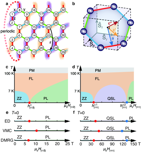
Fig. 1: Honeycomb lattice, crystalline directions, and phase diagrams. a shows the YC $W\times L\times 2$ honeycomb lattice of width $W=4$ and length $L$, with two sites per unit cell. The quasi-1D mapping path and site ordering is shown by the numbers, with the edge of each small hexagon set as length unit. In the zigzag magnetic order, spins align parallel along the highlighted lines, while anti-parallel between the yellow and purple lines. b shows an unit cell in $\alpha$-RuCl₃, with the a, $\textbf{c}^{*}$, and $\textbf{c}^{\prime}$ axes indicated. Finite-temperature phase diagrams under in-plane ($H_{[11\bar{2}]}\parallel\textbf{a}$) and out-of-plane ($H_{[111]}\parallel\textbf{c}^{*}$) fields are presented in c and d, respectively, with in-plane critical field $h^{c}_{[11\bar{2}]}\simeq 7$ T (computed at 1.9 K), and two out-of-plane critical fields $h^{c1}_{[111]}\approx 35$ T (lower) and $h^{c2}_{[111]}\approx 120$-130 T (upper), estimated at 0 K. In the phase diagrams, ZZ stands for the zigzag phase, PM for paramagnetic, FL for fractional liquid, and PL for the polarized phase, with the QPTs (red and blue points) indicated. e,f show the $T=0$ phase diagrams obtained by ED, VMC and DMRG, where the in-plane critical field is pinpointed at between 6.5 and 10 T, while two QPTs and a QSL phase are uncovered under out-of-plane fields.

We recall that the $\Gamma^{\prime}$ term is important for stabilizing the zigzag magnetic order at low temperature in the extended ferromagnetic (FM) Kitaev model with $K<0$ Kim and Kee (2016); Gordon et al. (2019); Lee et al. (2020). While the zigzag order can also be induced by the third-neighbor Heisenberg coupling $J_{3}$ Winter et al. (2016, 2017), we constrain ourselves within a minimal $K$-$J$-$\Gamma$-$\Gamma^{\prime}$ model in the present study and leave the discussion on the $J_{3}$ coupling in the Supplementary Note 1. In the simulations of $\alpha$-RuCl₃ under magnetic fields, we mainly consider the in-plane field along the $[11\bar{2}]$ direction, $H_{[11\bar{2}]}\parallel\textbf{a}$, and the out-of-plane field along the [111] direction, $H_{[111]}\parallel\textbf{c}^{*}$, with the corresponding Landé factors $g_{\rm ab}(=g_{[11\bar{2}]})$ and $g_{\rm c^{*}}(=g_{[111]})$, respectively. The index $[l,m,n]$ represents the field direction in the spin space depicted in Fig. 1b. Therefore, the Zeeman coupling between field $H_{[l,m,n]}$ to local moments can be written as $H_{\rm Zeeman}=g_{[l,m,n]}\mu_{\rm B}\mu_{0}H_{[l,m,n]}S_{i}^{[l,m,n]}$, where $S^{[l,m,n]}\equiv\mathbf{S}\cdot\mathbf{d}_{l,m,n}$ with $\mathbf{S}=(S_{x},S_{y},S_{z})$ and $\mathbf{d}_{l,m,n}=(l,m,n)^{T}/\sqrt{l^{2}+m^{2}+n^{2}}$. The site index $i=1,\cdots,N$, with $N\equiv W\times L\times 2$ the total site number.

In the simulations, various quantum many-body calculation methods have been employed (see Methods). The thermodynamic properties under zero and finite magnetic fields are computed by XTRG on finite-size systems (see, e.g, YC4 systems shown in Fig. 1a). The model parameters are pinpointed by fitting the XTRG results to the thermodynamic measurements, and then confirmed by the ground-state magnetization calculations by DMRG with the same geometry and VMC on an 8$\times$8$\times$2 torus. Moreover, the ED calculations of the dynamical properties are performed on a 24-site torus, which are in remarkable agreement to experiments and further strengthen the validity and accuracy of our spin model. Therefore, by combining these cutting-edge many-body approaches, we explain the experimental observations from the determined effective spin Hamiltonian, and explore the field-induced QSL in $\alpha$-RuCl₃ under magnetic fields.

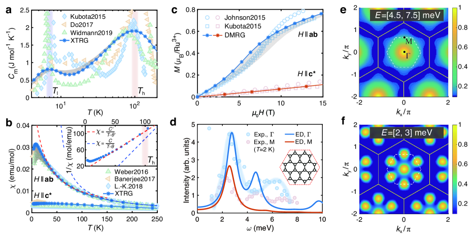
Fig. 2: Model simulations of thermodynamic and dynamic properties. With the $K$-$J$-$\Gamma$-$\Gamma^{\prime}$ model, we perform many-body simulations and compare the results to experiments, including a the magnetic specific heat $C_{\rm m}$ Kubota et al. (2015); Do et al. (2017); Widmann et al. (2019), b in-plane ($\chi_{\rm ab}$) and out-of-plane ($\chi_{\rm c^{*}}$) susceptibilities (measured at the field of 1 T) Lampen-Kelley et al. (2018); Banerjee et al. (2017); Weber et al. (2016), and c magnetization curves $M(H)$ Johnson et al. (2015); Kubota et al. (2015) on the YC4 $\times L\times$2 lattice, with the grey shaded region indicating the influences of different system lengths $L=4,6$. The Curie-Weiss fittings of the high- and intermediate-$T$ susceptibility $\chi_{\rm ab}$ in b lead to $C\simeq 0.67$ cm³K/mol, $\theta\simeq 41.4$ K, and $C^{\prime}\simeq 1.07$ cm³ K/mol, $\theta^{\prime}\simeq-12.7$ K, respectively. We also compute the dynamical spin structure by ED and compare the results with neutron scattering intensity $\mathcal{I}(\textbf{k},\omega)$ at $\textbf{k}=\Gamma$ and M in d, on a $C_{3}$ symmetric 24-site cluster shown in the inset (see more information and its comparison to another 24-site cluster with lower symmetry in the Supplementary Fig. 4). The light blue bold line is a guide to the eye for INS data at $\Gamma$ point Banerjee et al. (2018). The calculated intensity peak positions $\omega_{\Gamma}$ and $\omega_{\rm M}$ are in very good agreement with experiments. We further plot the integrated intensities within the energy interval e [4.5, 7.5] meV and f [2, 3] meV, where a clear M-star shape is reproduced in e at intermediate energy and the bright M points are evident in f at low energy, both in excellent agreement with the INS experiments Banerjee et al. (2017). The dashed white hexagon marks the first BZ, and the outer yellow hexagon is the extended BZ.

Model parameters. As shown in Fig. 2a-b, through simulating the experimental measurements, including the magnetic specific heat and both in- and out-of-plane susceptibility data Kubota et al. (2015); Do et al. (2017); Widmann et al. (2019); Lampen-Kelley et al. (2018); Banerjee et al. (2017); Weber et al. (2016); Johnson et al. (2015), we accurately determine the parameters in the Hamiltonian Eq. (1), which read $K=-25$ meV, $\Gamma=0.3\ |K|$, $\Gamma^{\prime}=-0.02\ |K|$, and $J=-0.1\ |K|$. The in- and out-of-plane Landé factors are found to be $g_{\rm ab}=2.5$ and $g_{\rm c^{*}}=2.3$, respectively. We find that both the magnetic specific heat $C_{\rm m}$ and the two susceptibilities (in-plane $\chi_{\rm ab}$ and out-of-plane $\chi_{\rm c^{*}}$) are quite sensitive to the $\Gamma$ term, and the inclusion of $\Gamma^{\prime}$($J$) term can significantly change the low-$T$ $C_{\rm m}$($\chi_{\rm ab}$) data. Based on these observations, we accurately pinpoint the various couplings. The details of parameter determination, with detailed comparisons to the previously proposed candidate models can be found in Supplementary Notes 1, 2. To check the robustness and uniqueness of the parameter fittings, we have also performed an automatic Hamiltonian searching Yu et al. with the Bayesian optimization combined large-scale thermodynamics solver XTRG, and find that the above effective parameter set indeed locates within the optimal regime of the optimization (Supplementary Note 1). In addition, the validity of our $\alpha$-RuCl₃ model is firmly supported by directly comparing the model calculations to the measured magnetization curves in Fig. 2c and INS measurements in Fig. 2d-f.

In our $K$-$J$-$\Gamma$-$\Gamma^{\prime}$ model of $\alpha$-RuCl₃, we see a dominating FM Kitaev interaction and a sub-leading positive $\Gamma$ term ($\Gamma>0$), which fulfill the interaction signs proposed from recent experiments Ran et al. (2017); Wu et al. (2018); Sears et al. (2020) and agree with some ab initio studies Kim and Kee (2016); Winter et al. (2017, 2017); Suzuki and Suga (2018); Laurell and Okamoto (2020). The strong Kitaev interaction seems to play a predominant role at intermediate temperature, which leads to the fractional liquid regime and therefore naturally explains the observed proximate spin liquid behaviors Banerjee et al. (2016, 2017); Do et al. (2017).

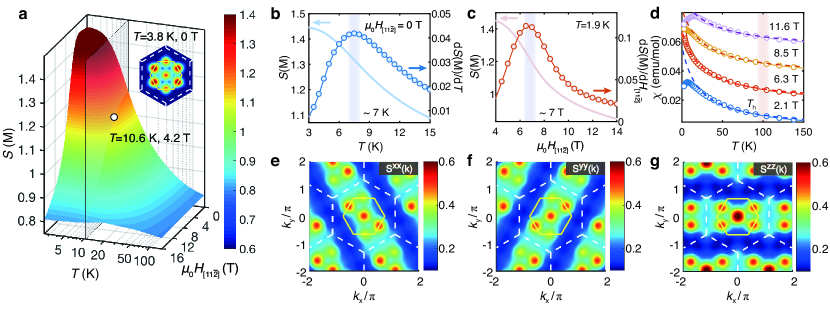
Fig. 3: Low-temperature zigzag order and intermediate-$T$ fractional liquid regime under in-plane fields $H_{[11\bar{2}]}\parallel\textbf{a}$. a Surface plot of the M-point spin structure factor $S(\rm{M})$ (average over six M points in the BZ) vs. temperature $T$ and field $H_{[11\bar{2}]}$. The inset is a low-$T$ structure factor with six bright M points in the BZ, representing the zigzag order. The $S(\rm{M})$ curve and its derivative over $T$ and $H_{[11\bar{2}]}$ are shown in b and c, respectively, which indicate a suppression of zigzag order at around the temperature $T_{\rm c}\simeq 7$ K and field $h^{c}_{[11\bar{2}]}\simeq 7$ T. d shows the emergent Curie-Weiss behavior in the magnetic susceptibility at intermediate $T$, with the fitted $C^{\prime}\simeq$ 1.17, 1.20, 1.21, and 1.27 $\rm{cm^{3}K/mol}$ and $\theta^{\prime}\simeq$ -20.7, -24.2, -26, and -34.4 K for fields $\mu_{0}H_{[11\bar{2}]}=$2.1, 6.3, 8.5 and 11.6 T, respectively. The different $\chi$ curves under various fields are shifted vertically by 0.018 emu/mol for clarify. The bright stripes of spin-resolved magnetic structure factors, i.e., $S^{xx}(\textbf{k})$, $S^{yy}(\textbf{k})$, and $S^{zz}(\textbf{k})$ as shown in e,f,g, respectively, calculated at $\mu_{0}H_{[11\bar{2}]}=4.2$ T and $T=10.6$ K, rotate counterclockwise (by 120^∘) as the spin component switches, reflecting the peculiar bond-oriented spin correlations in the intermediate fractional liquid regime.

Magnetic specific heat and two-temperature scales. We now show our simulations of the $K$-$J$-$\Gamma$-$\Gamma^{\prime}$ model and compare the results to the thermodynamic measurements. In Fig. 2a, the XTRG results accurately capture the prominent double-peak feature of the magnetic specific heat $C_{\rm m}$, i.e., a round high-$T$ peak at $T_{\rm h}\simeq 100$ K and a low-$T$ one at $T_{\rm l}\simeq 7$ K. As $T_{\rm h}\simeq 100$ K is a relatively high-temperature scale where the phonon background needs to be carefully deal with Widmann et al. (2019), and there exists quantitative difference among the various $C_{\rm m}$ measurements in the high-$T$ regime Kubota et al. (2015); Do et al. (2017); Widmann et al. (2019). Nevertheless, the high-$T$ scale $T_{\rm h}$ itself is relatively stable, and in Fig. 2a our XTRG result indeed exhibits a high-$T$ peak centered at around 100 K, in good agreement with various experiments. Note that the high-temperature crossover at $T_{\rm h}$ corresponds to the establishment of short-range spin correlations, which can be ascribed to the emergence of itinerant Majorana fermions Nasu et al. (2015); Do et al. (2017) in the fractional liquid picture that we will discuss. Such a crossover can also be observed in the susceptibilities, which deviate the high-$T$ Curie-Weiss law and exhibit an intermediate-$T$ Curie-Weiss scaling below $T_{\rm h}$ Li et al. (2020), as shown in Fig. 2b for $\chi_{\rm ab}$ (the same for $\chi_{\rm c^{*}}$).

At the temperature $T_{\rm l}\simeq 7$ K, the experimental $C_{\rm m}$ curves of $\alpha$-RuCl₃ exhibit a very sharp peak, corresponding to the establishment of a zigzag magnetic order Kubota et al. (2015); Do et al. (2017); Widmann et al. (2019); Sears et al. (2015); Banerjee et al. (2017). Such a low-$T$ scale can be accurately reproduced by our model calculations, as shown in Fig. 2a. As our calculations are performed on the cylinders of a finite width, the height of the $T_{\rm l}$ peak is less prominent than experiments, where the transition in the compound $\alpha$-RuCl₃ may be enhanced by the inter-layer couplings. Importantly, the location of $T_{\rm l}$ fits excellently to the experimental results. Below $T_{\rm l}$ our model indeed shows significantly enhanced zigzag spin correlation, which is evidenced by the low-energy dynamical spin structure in Fig. 2f and the low-$T$ static structure in the inset of Fig. 3a.

Anisotropic susceptibility and magnetization curves. It has been noticed from early experimental studies of $\alpha$-RuCl₃ that there exists a very strong magnetic anisotropy in the compound Sears et al. (2015); Kubota et al. (2015); Johnson et al. (2015); Weber et al. (2016); Banerjee et al. (2017); Lampen-Kelley et al. (2018); Sears et al. (2020), which was firstly ascribed to anisotropic Landé $g$ factor Kubota et al. (2015); Johnson et al. (2015), and recently to the existence of the off-diagonal $\Gamma$ interaction Lampen-Kelley et al. (2018); Sears et al. (2020). We compute the magnetic susceptibilities along two prominent field directions, i.e., $H_{[11\bar{2}]}$ and $H_{[111]}$, and compare them to experiments in Fig. 2b Weber et al. (2016); Banerjee et al. (2017); Lampen-Kelley et al. (2018). The discussions on different in-plane and tilted fields are left in the Supplementary Note 3.

In Fig. 2b, we show that both the in- and out-of-plane magnetic susceptibilities $\chi_{\rm ab}$ and $\chi_{\rm c^{*}}$ can be well fitted using our $K$-$J$-$\Gamma$-$\Gamma^{\prime}$ model, with dominant Kitaev $K$, considerable off-diagonal $\Gamma$, as well as similar in-plane ($g_{\rm ab}$) and out-of-plane ($g_{\rm c^{*}}$) Landé factors. Therefore, our many-body simulation results indicate that the anisotropic susceptibilities mainly originate from the off-diagonal $\Gamma$ coupling (cf. Supplementary Fig. 2), in consistent with the resonant elastic X-ray scattering Sears et al. (2020) and susceptibility measurements Lampen-Kelley et al. (2018). Moreover, with the parameter set of $K$, $\Gamma$, $\Gamma^{\prime}$, $J$, $g_{\rm ab}$, and $g_{\rm c^{*}}$ determined from our thermodynamics simulations, we compute the magnetization curves $M(H_{[l,m,n]})=1/N\sum_{i=1}^{N}g_{[l,m,n]}\mu_{\rm B}\langle S_{i}^{[l,m,n]}\rangle$ along the $[11\bar{2}]$ and [111] directions using DMRG, as shown in Fig. 2c. The two simulated curves, showing clear magnetic anisotropy, are in quantitative agreement with the experimental measurements at very low temperature Johnson et al. (2015); Kubota et al. (2015).

Dynamical spin structure and the M star. The INS measurements on $\alpha$-RuCl₃ revealed iconic dynamical structure features at low and intermediate energies Banerjee et al. (2017); Do et al. (2017). With the determined $\alpha$-RuCl₃ model, we compute the dynamical spin structure factors using ED, and compare the results to experiments. Firstly, we show in Fig. 2d the constant k-cut at the $\textbf{k}=\Gamma$ and M points (as indicated in Fig. 2e), where a quantitative agreement between theory and experiment can be observed. In particular, the positions of the intensity peak $\omega_{\Gamma}=2.69\pm 0.11$ meV and $\omega_{\rm M}=2.2\pm 0.2$ meV from the INS measurements Banerjee et al. (2017), are accurately reproduced with our determined model. For the $\Gamma$-point intensity, the double-peak structure, which was observed in experimental measurements Banerjee et al. (2018), can also be well captured.

We then integrate the INS intensity $\mathcal{I}(\textbf{k},\omega)$ over the low- and intermediate-energy regime with the atomic form factor taken into account, and check their k-dependence in Fig. 2e-f. In experiment, a structure factor with bright $\Gamma$ and M points was observed at low energy, and, on the other hand, a renowned six-pointed star shape (dubbed M star Laurell and Okamoto (2020)) was reported at intermediate energies Banerjee et al. (2017); Do et al. (2017). In Fig. 2e-f, these two characteristic dynamical spin structures are reproduced, in exactly the same energy interval as experiments. Specifically, the zigzag order at low temperature is reflected in the bright M points in the Brillouin zone (BZ) when integrated over [2, 3] meV, and the $\Gamma$ point in the BZ is also turned on. As the energy interval increases to [4.5, 7.5] meV, the M star emerges as the zigzag correlation is weakened while the continuous dispersion near the $\Gamma$ point remains prominent. The round $\Gamma$ peak, which also appears in the pure Kitaev model, is consistent with the strong Kitaev term in our $\alpha$-RuCl₃ model.

Suppressing the zigzag order by in-plane fields. In experiments, the low-$T$ zigzag magnetic order has been observed to be suppressed by the in-plane magnetic fields above 7-8 T Kubota et al. (2015); Johnson et al. (2015); Zheng et al. (2017); Banerjee et al. (2018). We hereby investigate this field-induced effect by computing the spin structure factors under finite fields. The M-point peak of the structure factor $S(\rm M)$ in the $T$-$H_{[11\bar{2}]}$ plane characterizes the zigzag magnetic order as shown in Fig. 3a. The derivatives $\frac{dS({\rm M})}{dT}|_{H=0}$ and $\frac{dS({\rm M})}{dH}|_{T=1.9~{}\rm{K}}$ are calculated in Fig. 3b-c, which can only show a round peak at the transition as limited by our finite-size simulation. For $H=0$, the turning temperature is at about $7$ K, below which the zigzag order builds up; on the other hand, the isothermal $M$-$H$ curves in Fig. 3c suggest a transition point at $h_{[11\bar{2}]}^{c}=\mu_{0}H_{[11\bar{2}]}\simeq 7$ T, beyond which the zigzag order is suppressed. Correspondingly, in Fig. 4c [and also in Fig. 4d], the low-temperature scale $T_{\rm l}$ decreases as the fields increase, initially very slow for small fields and then quickly approaches zero only in the field regime near the critical point, again in very good consistency with experimental measurements Kubota et al. (2015); Zheng et al. (2017); Baek et al. (2017).

Besides, from the contour plots of $C_{\rm m}/T$ and the isentropes in Fig. 4a, c, one can also recognize the critical temperature and field consistent with the above estimations. Moreover, when the field direction is tilted about $55^{\circ}$ away from the a axis in the a-$\textbf{c}^{*}$ plane (i.e., $H_{[110]}$ along the $c^{\prime}$ axis), as shown in Fig. 4b, d, our model calculations suggest a critical field $h_{[110]}^{c}=\mu_{0}H_{[110]}\simeq 10$ T with suppressed zigzag order, in accordance with recent NMR probe Baek et al. (2017). Overall, the excellent agreements of the finite-field simulations with different experiments further confirm our $K$-$J$-$\Gamma$-$\Gamma^{\prime}$ model as an accurate description of the Kitaev material $\alpha$-RuCl₃.

Finite-$T$ phase diagram under in-plane fields. Despite intensive experimental and theoretical studies, the phase diagram of $\alpha$-RuCl₃ under in-plane fields remains an interesting open question. The thermal Hall Kasahara et al. (2018b), Raman scattering Wulferding et al. (2020), and thermal expansion Gass et al. (2020) measurements suggest the existence of an intermediate QSL phase between the zigzag and polarized phases. On the other hand, the magnetization Kubota et al. (2015); Johnson et al. (2015), INS Banerjee et al. (2018), NMR Zheng et al. (2017); Baek et al. (2017); Janša et al. (2018), ESR Ponomaryov et al. (2020), Grüneisen parameter Bachus et al. (2020), and magnetic torque measurements Modic et al. (2021) support a single-transition scenario (leaving aside the transition between two zigzag phases due to different inter-layer stackings Balz et al. (2019)). Nevertheless, most experiments found signatures of fractional excitations at finite temperature, although an alternative multi-magnon interpretation has also been proposed Ponomaryov et al. (2020).

Fig. 4: Contour plots of $C_{\rm m}/T$ and the isentropes. The magnetic specific heat $C_{\rm m}/T$ under $H_{[11\bar{2}]}\parallel\textbf{a}$ and $H_{[110]}\parallel\textbf{c}^{\prime}$ are shown in panels a and b, respectively. The white dashed lines indicate the low-temperature scale $T_{\rm l}$ and $T_{\rm l}^{\prime}$ and are guides for the eye. The red dots on the $T=0$ axis denote the QPT at $h_{[11\bar{2}]}^{c}\simeq 7$ T and $h_{[110]}^{c}\simeq 10$ T. The isentropes along the two field directions are shown in panels c and d, where we find an intermediate regime with fractional thermal entropies $\sim(\ln{2})/2$.

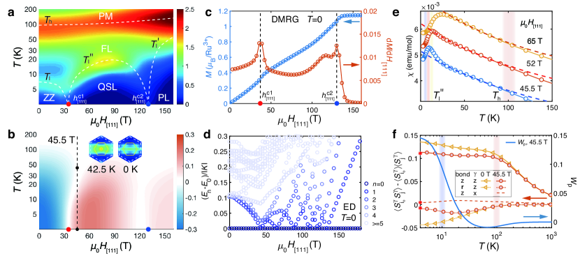
Fig. 5: Quantum spin liquid regime of $\alpha$-RuCl₃ model under the out-of-plane field $H_{[111]}\parallel$ c^∗. a Color map of the specific heat $C_{\rm m}$, where a double-peak feature appears at both low and intermediate fields. The white dashed lines, with $T_{\rm h}$, $T_{\rm l}$, and $T^{\prime\prime}_{\rm l}$ determined from the specific heat and $T^{\prime}_{\rm l}$ from spin structure (cf. Supplementary Note 4), represent the phase boundaries and are guides for the eye. b shows the $Z_{2}$ flux $W_{\rm p}$, where the regime with positive(negative) $W_{\rm p}$ is plotted in orange(blue). The zero and finite-temperature spin structure factors $\tilde{S}^{zz}(\textbf{k})$ (see main text) at $\mu_{0}H_{[111]}=45.5$ T are shown in the inset of b and plotted with the same colorbar as that in Fig. 3e-g. c shows the $T=0$ magnetization curve and its derivative d$M$/d$H_{[111]}$, where the two peaks can be clearly identified at $\mu_{0}H_{[111]}\simeq$ 35 and 130 T, respectively. The two transition fields, marked by $h_{[111]}^{c1}$ and $h_{[111]}^{c2}$, are also indicated in panels a and b. d ED Energy spectra $E_{\rm n}{\rm-}E_{\rm 0}$ under $H_{[111]}$ fields, with gapless low-energy excitations emphasized by dark colored symbols. e The magnetic susceptibility with an intermediate-$T$ Curie-Weiss behavior, with the fitted $C^{\prime}\simeq$ 1.22, 1.14, and 1.00 $\rm{cm^{3}K/mol}$ and $\theta^{\prime}\simeq$ -236.8, -217.8, and -187.4 K, for fields $\mu_{0}H_{[111]}=$45.5, 52 and 65 T, respectively. The susceptibility curves in e are shifted vertically by a constant 0.001 emu/mol for clarify. f shows the temperature dependence of the spin correlations (left $y$-axis) and the flux $W_{\rm p}$ (right $y$-axis), where the correlations $\langle S_{i_{0}}^{z}S_{j}^{z}\rangle$- $\langle S^{z}_{i_{0}}\rangle\langle S^{z}_{j}\rangle$ are measured on both $z$- and r-bonds [see Fig. 1a], and $\langle S_{i_{0}}^{x}S_{j}^{x}\rangle$- $\langle S^{x}_{i_{0}}\rangle\langle S^{x}_{j}\rangle$ on the $z$-bond, under two different fields of 0 and 45.5 T (with $i_{0}$ a fixed central reference site). The low-$T$ XTRG data are shown to converge to the $T=0$ DMRG results, with the latter marked as red asterisks on the left vertical axis. The flux expectation $W_{\rm p}$ are measured under $\mu_{0}H_{[111]}=45.5$ T, which increases rapidly around low-$T$ scale $T^{\prime\prime}_{\rm l}$.

Now with the accurate $\alpha$-RuCl₃ model and multiple many-body computation techniques, we aim to determine the phase diagram and nature of the field-driven phase(s). Our main results are summarized in Fig. 1c, e, where a single quantum phase transition (QPT) is observed as the in-plane fields $H_{[11\bar{2}]}$ increases. Both VMC and DMRG calculations find a trivial polarized phase in the large-field side ($\mu_{0}H_{[11\bar{2}]}>h_{[11\bar{2}]}^{c}$), as evidenced by the magnetization curve in Fig. 2c as well as the results in Supplementary Note 3.

Despite the QSL phase is absent under in-plane fields, we nevertheless find a Kitaev fractional liquid at finite temperature, whose properties are determined by the fractional excitations of the system. For the pure Kitaev model, it has been established that the itinerant Majorana fermions and $Z_{2}$ fluxes each releases half of the entropy at two crossover temperature scales Nasu et al. (2015); Do et al. (2017). Such an intriguing regime is also found robust in the extended Kitaev model with additional non-Kitaev couplings Li et al. (2020). Now for the realistic $\alpha$-RuCl₃ model in Eq. (1), we find again the presence of fractional liquid at intermediate $T$. As shown in Fig. 2b (zero field) and Fig. 3d (finite in-plane fields), the intermediate-$T$ Curie-Weiss susceptibility can be clearly observed, with the fitted Curie constant $C^{\prime}$ distinct from the high-$T$ paramagnetic constant $C$. This indicates the emergence of a novel correlated paramagnetism — Kitaev paramagnetism — in the material $\alpha$-RuCl₃. The fractional liquid constitutes an exotic finite-temperature quantum state with disordered fluxes and itinerant Majorana fermions, driven by the strong Kitaev interaction that dominates the intermediate-$T$ regime Li et al. (2020).

In Fig. 4c-d of the isentropes, we find that the Kitaev fractional liquid regime is rather broad under either in-plane ($H_{[11\bar{2}]}$) or tilted ($H_{[110]}$) fields. When the field is beyond the critical value, the fractional liquid regime gradually gets narrowed, from high-$T$ scale $T_{\rm h}$ down to a new lower temperature scale $T^{\prime}_{\rm l}$, below which the field-induced uniform magnetization builds up (see Supplementary Note 3). From the specific heat and isentropes in Fig. 4, we find in the polarized phase $T^{\prime}_{\rm l}$ increases linearly as field increases, suggesting that such a low-$T$ scale can be ascribed to the Zeeman energy. At the intermediate temperature, the thermal entropy is around $(\ln{2})/2$ [see Fig. 4c-d], indicating that “one-half” of the spin degree of freedom, mainly associated with the itinerant Majorana fermions, has been gradually frozen below $T_{\rm h}$.

Besides, we also compute the spin structure factors $S^{\gamma\gamma}(\textbf{k})={1}/{N_{\rm Bulk}}\,\sum_{i,j\in{\rm Bulk}}e^{i\textbf{k}(\textbf{r}_{j}-\textbf{r}_{i})}\langle S^{\gamma}_{i}S^{\gamma}_{j}\rangle$ under an in-plane field of $\mu_{0}H_{[11\bar{2}]}=4.2$ T in the fractional liquid regime, where ${N_{\rm Bulk}}$ is the number of bulk sites (with left and right outmost columns skipped), $i,j$ run over the bulk sites, and $\gamma=x,y,z$. Except for the bright spots at $\Gamma$ and M points, there appears stripy background in Fig. 3e-g very similar to that observed in the pure Kitaev model Li et al. (2020), which reflects the extremely short-range and bond-directional spin correlations there. The stripe rotates as the spin component $\gamma$ switches, because the $\gamma$-type spin correlations $\langle S^{\gamma}_{i}S^{\gamma}_{j}\rangle_{\gamma}$ are nonzero only on the nearest-neighbor $\gamma$-type bond. As indicated in the realistic model calculations, we propose such distinct features in $S^{\gamma\gamma}(\textbf{k})$ can be observed in the material $\alpha$-RuCl₃ via the polarized neutron diffusive scatterings.

Signature of Majorana fermions and the Kitaev fractional liquid. It has been highly debated that whether there exists a QSL phase under intermediate in-plane fields. Although more recent experiments favor the single-transition scenario Bachus et al. (2020); Modic et al. (2021), there is indeed signature of fractional Majorana fermions and spin liquid observed in the intermediate-field regime Banerjee et al. (2018); Kasahara et al. (2018b); Janša et al. (2018); Wulferding et al. (2020); Modic et al. (2021). Based on the model simulations, here we show that our finite-$T$ phase diagram in Fig. 1 provides a consistent scenario that reconciles these different in-plane field experiments.

For example, large Kasahara et al. (2018a); Hentrich et al. (2019) or even half-quantized thermal Hall conductivity was observed at intermediate fields and between 4-6 K Kasahara et al. (2018c); Yamashita et al. (2020); Yokoi et al. . However, it has also been reported that the thermal Hall conductivity vanishes rapidly when the field further varies or the temperature lowers below approximately 2 K Czajka et al. (2021). Therefore, one possible explanation, according to our model calculations, is that the ground state under in-plane fields above $7$ T is a trivial polarized phase [see Fig. 1c], while the large thermal Hall conductivity at intermediate fields may originate from the Majorana fermion excitations in the finite-$T$ fractional liquid Nasu et al. (2015).

In the intermediate-$T$ fractional liquid regime, the Kitaev interaction is predominating and the system resembles a pure Kitaev model under external fields and at a finite temperature. This effect is particularly prominent as the field approaches the intermediate regime, i.e., near the quantum critical point, where the fractional liquid can persist to much lower temperature. Matter of fact, given a fixed low temperature, when the field is too small or too large, the system leaves the fractional liquid regime (cf. Fig. 4) and the signatures of the fractional excitation become blurred, as if there were a finite-field window of “intermediate spin liquid phase”. Such fractional liquid constitutes a Majorana metal state with a Fermi surface Nasu et al. (2015); Li et al. (2020), accounting possibly for the observed quantum oscillation in longitudinal thermal transport Czajka et al. (2021). Besides thermal transport, the fractional liquid dominated by fractional excitations can lead to rich experimental ramifications, e.g., the emergent Curie-Weiss susceptibilities in susceptibility measurements [see Fig. 3d] and the stripy spin structure background in the spin-resolved neutron or resonating X-ray scatterings [Fig. 3e-g], which can be employed to probe the finite-$T$ fractional liquid in the compound $\alpha$-RuCl₃.

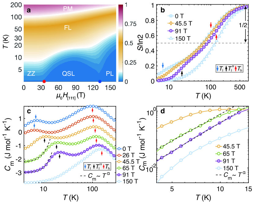
Fig. 6: Fractional entropy and specific heat under out-of-plane fields. a The contour plot of thermal entropy $S$/ln2, where the two critical fields (red and blue dots) are clearly signaled by the two dips in the isentropic lines. The entropy curves $S(T)$ are shown in b, where half of the entropy $\Delta S=(\ln{2})/2$ is released around the high temperature scale $T_{\rm h}$, while the rest half released either by forming zigzag order (below $h_{[111]}^{c1}$, see, e.g., the 0 T curve), or freezing $Z_{2}$ flux (between $h_{[111]}^{c1}$ and $h_{[111]}^{c2}$, e.g., the 45.5 T and 91 T curves), at the lower-temperature scale $T_{\rm l}$ and $T^{\prime\prime}_{\rm l}$ denoted by the arrows. For field above $h_{[111]}^{c2}$ the system gradually crossover to the polarized states at low temperature. c shows the specific heat $C_{\rm m}$ curves under various fields, with the blue(black) arrows indicating the low-$T$ scales $T_{\rm l}$($T^{\prime\prime}_{\rm l}$), and the red arrows for $T_{\rm h}$ which increases as the field enhances. The $C_{\rm m}$ curves are shifted vertically by a constant 0.75 J mol^-1 K^-1 for clarify. In the QSL regime, the low-$T$ specific heat show algebraic behaviors in c, also zoomed in and plotted with log-log scale in d, and we plot a power-law $C_{\rm m}\sim T^{\alpha}$ in both panels as guides for the eye, with $\alpha$ estimated to be around 2.8-3.4 based on our YC4 calculations.

Quantum spin liquid induced by out-of-plane fields. Now we apply the $H_{[111]}\parallel\textbf{c}^{*}$ field out of the plane and investigate the field-induced quantum phases in $\alpha$-RuCl₃. As shown in the phase diagram in Fig. 1d, f, under the $H_{[111]}$ fields a field-induced QSL phase emerges at intermediate fields between the zigzag and the polarized phases, confirmed in both the thermal and ground-state calculations. The existence of two QPTs and an intermediate phase can also be seen from the color maps of $C_{\rm m}$, $Z_{2}$ fluxes, and thermal entropies shown in Figs. 5a-b and 6a.

To accurately nail down the two QPTs, we plot the $\textbf{c}^{*}$ DMRG magnetization curve $M(H_{[111]})$ and the derivative $dM/dH_{[111]}$ in Fig. 5c, together with the ED energy spectra in Fig. 5d, from which the ground-state phase diagram can be determined (cf. Fig. 1f). In particular, the lower transition field, $h_{[111]}^{c1}\simeq 35$ T, estimated from both XTRG and DMRG, is in excellent agreement with recent experiment through measuring the magnetotropic coefficient Modic et al. (2021). The existence of the upper critical field $h_{[111]}^{c2}$ at 100 T level can also be probed with current pulsed high field techniques Zhou and Matsuda (2020).

Correspondingly, we find in Fig. 5b that the $Z_{2}$ flux $W_{\rm p}=2^{6}\langle S_{i}^{x}S_{j}^{y}S_{k}^{z}S_{l}^{x}S_{m}^{y}S_{n}^{z}\rangle$ (where $i,j,k,l,m,n$ denote the six vertices of a hexagon $p$) changes its sign from negative to positive at $h_{[111]}^{c1}$, then to virtually zero at $h_{[111]}^{c2}$, and finally converge to very small (positive) values in the polarized phase. These observations of flux signs in different phases are consistent with recent DMRG and tensor network studies on a $K$-$\Gamma$-$\Gamma^{\prime}$ model Gordon et al. (2019); Lee et al. (2020), and it is noteworthy that the flux is no longer a strictly conserved quantity as in the pure Kitaev model, the low-$T$ expectation values of $|W_{\rm p}|$ thus would be very close to $1$ only deep in the Kitaev spin liquid phase Gordon et al. (2019); Hickey and Trebst (2019); Li et al. (2020).

From the $C_{\rm m}$ color map in Fig. 5a and $C_{\rm m}$ curves in Fig. 6c, we find double-peaked specific heat curves in the QSL phase, which clearly indicate the two temperature scales, e.g., $T_{\rm h}\simeq 105$ K and $T^{\prime\prime}_{\rm l}\simeq 10$ K for $\mu_{0}H_{[111]}=45.5$ T. They correspond to the establishment of spin correlations at $T_{\rm h}$ and the alignment of $Z_{2}$ fluxes at $T^{\prime\prime}_{\rm l}$, respectively, as shown in Fig. 5f. As a result, in Fig. 6a-b the system releases $(\ln{2})/2$ thermal entropy around $T_{\rm h}$, and the rest half is released at around $T^{\prime\prime}_{\rm l}$. The magnetic susceptibility curves in Fig. 5e fall into an intermediate-$T$ Curie-Weiss behavior below $T_{\rm h}$ when the spin correlations are established, and deviate such emergent universal behavior when approaching $T^{\prime\prime}_{\rm l}$ as the gauge degree of freedom (flux) gradually freezes.

Furthermore, we study the properties of the QSL phase. We find very peculiar spin correlations as evidenced by the (modified) structure factor

$$\tilde{S}^{zz}(\textbf{k})=\frac{1}{N_{{\rm Bulk}}}\sum_{i,j\in{\rm Bulk}}e^{i\textbf{k}(\textbf{r}_{j}-\textbf{r}_{i})}(\langle S_{i}^{z}S_{j}^{z}\rangle-\langle S^{z}_{i}\rangle\langle S^{z}_{j}\rangle).$$ (2)

As shown in the inset of Fig. 5b, there appears no prominent peak in $\tilde{S}^{zz}(\textbf{k})$ at both finite and zero temperatures, for a typical field of $45.5$ T in the QSL phase. As shown in Fig. 5f, we find the dominating nearest-neighboring correlations at $T>0$ are bond-directional and the longer-range correlations are rather weak, same for the QSL ground state at $T=0$. This is in sharp contrast to the spin correlations in the zigzag phase. More spin structure results computed with both XTRG and DMRG can be found in Supplementary Note 4. Below the temperature $T^{\prime\prime}_{\rm l}$, we observe an algebraic specific heat behavior as shown in Fig. 6c-d, which strongly suggests a gapless QSL. We remark that the gapless spin liquid in the pure Kitaev model also has bond-directional and extremely short-range spin correlations Kitaev (2006). The similar features of spin correlations in this QSL state may be owing to the predominant Kitaev interaction in our model.

Overall, under the intermediate fields between $h_{[111]}^{c1}$ and $h_{[111]}^{c2}$, and below the low-temperature scale $T^{\prime\prime}_{\rm l}$, our model calculations predict the presence of the long-been-sought QSL phase in the compound $\alpha$-RuCl₃.

Discussion
Firstly, we discuss the nature of the QSL driven by the out-of-plane fields. In Fig. 5d, the ED calculation suggests a gapless spectrum in the intermediate phase, and the DMRG simulations on long cylinders find the logarithmic correction in the entanglement entropy scaling (see Supplementary Note 4), which further supports a gapless QSL phase. On the other hand, the VMC calculations identify the intermediate phase as an Abelian chiral spin liquid, which is topologically nontrivial with a quantized Chern number $\nu=2$. Overall, various approaches consistently find the same scenario of two QPTs and an intermediate-field QSL phase under high magnetic fields [cf. Fig. 1d, f]. It is worth noticing that a similar scenario of a gapless QSL phase induced by out-of-plane fields has also been revealed in a Kitaev-Heisenberg model with $K>0$ and $J<0$ Jiang et al. (2019), where the intermediate QSL was found to be smoothly connected to the field-induced spin liquid in a pure AF Kitaev model Zhu et al. (2018); Hickey and Trebst (2019); Patel and Trivedi (2019). We note the extended AF Kitaev model in Ref. Jiang et al. (2019) can be transformed into a $K$-$J$-$\Gamma$-$\Gamma^{\prime}$ model with FM Kitaev term (and other non-Kitaev terms still distinct from our model) through a global spin rotation Chaloupka and Khaliullin (2015). Therefore, despite the rather different spin structure factors of the field-induced QSL in the AF Kitaev model from ours, it is interesting to explore the possible connections between the two in the future.

Based on our $\alpha$-RuCl₃ model and precise many-body calculations, we offer concrete experimental proposals for detecting the intermediate QSL phase via the magnetothermodynamic measurements under high magnetic fields. The two QPTs are within the scope of contemporary technique of pulsed high fields, and can be confirmed by measuring the magnetization curves Zhou et al. ; Zhou and Matsuda (2020). The specific heat measurements can also be employed to confirm the two-transition scenario and the high-field gapless QSL states. As field increases, the lower temperature scale $T_{\rm l}$ first decreases to zero as the zigzag order is suppressed, and then rises up again (i.e., $T^{\prime\prime}_{\rm l}$) in the QSL phase [cf. Fig. 5a]. As the specific heat exhibits a double-peak structure in the high-field QSL regime, the thermal entropy correspondingly undergoes a two-step release in the QSL phase and exhibits a quasi-plateau near the fractional entropy $(\ln{2})/2$ [cf. 45.5 T and 91 T lines in Fig. 6b]. This, together with the low-$T$ (below $T^{\prime\prime}_{\rm l}$) algebraic specific heat behavior reflecting the gapless excitations, can be probed through high-field calorimetry Imajo et al. .

Lastly, it is interesting to note that the emergent high-field QSL under out-of-plane fields may be closely related to the off-diagonal $\Gamma$ term (see, e.g., Refs. Gordon et al. (2019); Lee et al. (2020)) in the compound $\alpha$-RuCl₃. The $\Gamma$ term has relatively small influences in ab plane, while introduces strong effects along the $\textbf{c}^{*}$ axis — from which the magnetic anisotropy in $\alpha$-RuCl₃ mainly originates. The zigzag order can be suppressed by relatively small in-plane fields and the system enters the polarized phase, as the $\Gamma$ term does not provide a strong “protection” of both zigzag and QSL phases under in-plane fields (recall the QSL phase in pure FM Kitaev model is fragile under external fields Jiang et al. (2011); Hickey and Trebst (2019); Li et al. (2020)). The situation is very different for out-of-plane fields, where the Kitaev (and also Gamma) interactions survive the QSL after the zigzag order is suppressed by high fields. Intuitively, the emergence of this QSL phase can therefore be ascribed to the strong competition between the $\Gamma$ interaction and magnetic field along the hard axis $\textbf{c}^{*}$ of $\alpha$-RuCl₃. With such insight, we expect a smaller critical field for compounds with a less significant $\Gamma$ interaction. In the fast-moving Kitaev materials studies, such compounds with relatively weaker magnetic anisotropy, e.g., the recent Na₂Co₂TeO₆ and Na₂Co₂SbO₆ Yao and Li (2020); Hong et al. ; Lin et al. ; Songvilay et al. (2020), have been found, which may also host QSL induced by out-of-plane fields at lower field strengths.

Methods
Exponential tensor renormalization group. The thermodynamic quantities including the specific heat, magnetic susceptibility, $Z_{2}$ flux, and the spin correlations can be computed with the exponential tensor renormalization group (XTRG) method Chen et al. (2018); Li et al. (2019) on the Y-type cylinders with width $W=4$ and length up to $L=6$ (i.e., YC4$\times$6$\times$2). We retain up to $D=800$ states in the XTRG calculations, with truncation errors $\epsilon\lesssim 2\times 10^{-5}$, which guarantees a high accuracy of computed thermal data down to the lowest temperature $T\simeq 1.9$ K. Note the truncation errors in XTRG, different from that in DMRG, directly reflects the relative errors in the free energy and other thermodynamics quantities. The low-$T$ data are shown to approach the $T=0$ DMRG results (see Fig. 5f). In the thermodynamics simulations of the $\alpha$-RuCl₃ model, one needs to cover a rather wide range of temperatures as the high- and low-$T$ scales are different by more than one order of magnitude (100 K vs. 7 K in $\alpha$-RuCl₃ under zero field). In the XTRG cooling procedure, we represent the initial density matrix $\rho_{0}(\tau)$ at a very high temperature $T\equiv 1/\tau$ (with $\tau\ll 1$) as a matrix product operator (MPO), and the series of lower temperature density matrices $\rho_{n}(2^{n}\tau)$ ($n\geq 1$) are obtained by successively multiplying and compressing $\rho_{n}=\rho_{n-1}\cdot\rho_{n-1}$ via the tensor-network techniques. Thus XTRG is very suitable to deal with such Kitaev model problems, as it cools down the system exponentially fast in temperature Li et al. (2020).

Density matrix renormalization group. The ground state properties are computed by the density matrix renormalization group (DMRG) method, which can be considered as a variational algorithm based on the matrix product state (MPS) ansatz. We keep up to $D=2048$ states to reduce the truncation errors $\epsilon\lesssim 1\times 10^{-8}$ with a very good convergence. The simulations are based on the high-performance MPS algorithm library GraceQ/MPS2 Sun and Peng .

Variational Monte Carlo. The ground state of $\alpha$-RuCl₃ model are evaluated by the variational Monte Carlo (VMC) method based on the fermionic spinon representation. The spin operators are written in quadratic forms of fermionic spinons $S_{i}^{m}=\frac{1}{2}C_{i}^{\dagger}\sigma^{m}C_{i},m=x,y,z$ under the local constraint $\hat{N}_{i}=c_{i\uparrow}^{\dagger}c_{i\uparrow}+c_{i\downarrow}^{\dagger}c_{i\downarrow}=1$, where $C_{i}^{\dagger}=(c_{i\uparrow}^{\dagger},c_{i\downarrow}^{\dagger})$ and $\sigma^{m}$ are Pauli matrices. Through this mapping, the spin interactions are expressed in terms of fermionic operators and are further decoupled into a non-interacting mean-field Hamiltonian $H_{\rm mf}(\boldsymbol{R})$, where $\boldsymbol{R}$ denotes a set of parameters (see Supplementary Note 5). Then we perform Gutzwiller projection to the mean-field ground state $|\Phi_{\rm mf}(\boldsymbol{R})\rangle$ to enforce the particle number constraint ($\hat{N}_{i}=1$). The projected states $|\Psi(\boldsymbol{R})\rangle=P_{G}|\Phi_{\rm mf}(\boldsymbol{R})\rangle=\sum_{\alpha}f(\alpha)|\alpha\rangle$ (here $\alpha$ stands for the Ising bases in the many-body Hilbert space, same for $\beta$ and $\gamma$ below) provide a series of trial wave functions, depending on the specific choice of the mean-field Hamiltonian $H_{\rm mf}(\boldsymbol{R})$. Owing to the huge size of the many-body Hilbert space, the energy of the trial state $E(\boldsymbol{R})=\langle\Psi(\boldsymbol{R})|H|\Psi(\boldsymbol{R})\rangle/\langle\Psi(\boldsymbol{R})|\Psi(\boldsymbol{R})\rangle=\sum_{\alpha}{|f(\alpha)|^{2}\over\sum_{\gamma}|f(\gamma)|^{2}}\Big{(}\sum_{\beta}\langle\beta|H|\alpha\rangle{f(\beta)^{*}\over f(\alpha)^{*}}\Big{)}$ is computed using Monte Carlo sampling. The optimal parameters $\boldsymbol{R}$ are determined by minimizing the energy $E(\boldsymbol{R})$. While the VMC calculations are performed on a relatively small size (up to $128$ sites), once the optimal parameters are determined we can plot the spinon dispersion of a QSL state by diagonalizing the mean-field Hamiltonian on a larger lattice size, e.g., $120\times 120$ unit cells in practice.

Exact diagonalization. The 24-site exact diagonalization (ED) is employed to compute the zero-temperature dynamical correlations and energy spectra. The clusters with periodic boundary conditions are depicted in the inset of Fig. 2d and the Supplementary Information, and the $\alpha$-RuCl₃ model under in-plane fields ($H_{[11\bar{2}]}\parallel\textbf{a}$ and $H_{[1\bar{1}0]}\parallel\textbf{b}$) as well as out-of-plane fields $H_{[111]}\parallel\textbf{c}^{*}$ have been calculated, as shown in Fig. 5 and Supplementary Note 3. Regarding the dynamical results — the neutron scattering intensity — is defined as

$$\begin{split}\mathcal{I}(\textbf{k},\omega)\varpropto&f^{2}(\textbf{k})\int dt\sum_{\mu,\nu}(\delta_{\mu,\nu}-k_{\mu}k_{\nu}/k^{2})\\ &\times\sum_{i,j}\langle S_{i}^{\mu}(t)S_{j}^{\nu}(0)\rangle e^{i\textbf{k}\cdot(\textbf{r}_{j}-\textbf{r}_{i})}e^{-i\omega t},\\ \end{split}$$ (3)

where $f(\textbf{k})$ is the atomic form factor of Ru³⁺, which can be fitted by an analytical function as reported in Ref. Cromer and Waber (1965). $S^{\mu\nu}(\textbf{k},\omega)=\sum_{i,j}\langle S_{i}^{\mu}(t)S_{j}^{\nu}(0)\rangle e^{i\textbf{k}\cdot(\textbf{r}_{j}-\textbf{r}_{i})}e^{-i\omega t}$ is the dynamical spin structure factor, which can be expressed by the continued fraction expansion in the tridiagonal basis of the Hamiltonian using Lanczos iterative method. For the diagonal part,

$$\begin{split}S^{\mu\mu}(\textbf{k},\omega)&=-\frac{1}{\pi}{\rm Im}{\Big{[}}\langle\psi_{0}|\hat{S}^{\mu}_{-\textbf{k}}\frac{1}{z-\hat{H}}\hat{S}^{\mu}_{\textbf{k}}|\psi_{0}\rangle{\Big{]}}\\ &=-\frac{1}{\pi}{\rm Im}{\Bigg{[}}\frac{\langle\psi_{0}|\hat{S}^{\mu}_{-\textbf{k}}\hat{S}^{\mu}_{\textbf{k}}|\psi_{0}\rangle}{z-a_{0}-\frac{b_{1}^{2}}{z-a_{1}-\frac{b_{2}^{2}}{z-a_{2}-\cdot\cdot\cdot}}}{\Bigg{]}},\\ \end{split}$$ (4)

where $z=\omega+E_{0}+i\eta$, $E_{0}$ is the ground state energy, $|\psi_{0}\rangle$ is the ground state wave function, $\eta$ is the Lorentzian broadening factor (here we take $\eta=0.5$ meV in the calculations, i.e., 0.02 times the Kitaev interaction strength $|K|=$25 meV), and $a_{i}$ ($b_{i+1}$) is the diagonal (sub-diagonal) matrix element of the tridiagonal Hamiltonian. On the other hand, for the off-diagonal part, we define a Hermitian operator $\hat{S}_{\textbf{k}}^{\mu}+\hat{S}_{\textbf{k}}^{\nu}$ to do the continued fraction expansion,

$$\begin{split}&S^{(\mu+\nu)(\mu+\nu)}(\textbf{k},\omega)\\ &\hskip 8.53581pt=-\frac{1}{\pi}{\rm Im}{\Big{[}}\langle\psi_{0}|(\hat{S}^{\mu}_{-\textbf{k}}+\hat{S}^{\nu}_{-\textbf{k}})\frac{1}{z-\hat{H}}(\hat{S}^{\mu}_{\textbf{k}}+\hat{S}^{\nu}_{\textbf{k}})|\psi_{0}\rangle{\Big{]}}\\ &\hskip 8.53581pt=-\frac{1}{\pi}{\rm Im}{\Bigg{[}}\frac{\langle\psi_{0}|(\hat{S}^{\mu}_{-\textbf{k}}+\hat{S}^{\nu}_{-\textbf{k}})(\hat{S}^{\mu}_{\textbf{k}}+\hat{S}^{\nu}_{\textbf{k}})|\psi_{0}\rangle}{z-a_{0}-\frac{b_{1}^{2}}{z-a_{1}-\frac{b_{2}^{2}}{z-a_{2}-\cdot\cdot\cdot}}}{\Bigg{]}}.\\ \end{split}$$ (5)

Then the off-diagonal $S^{\mu\nu}(\textbf{k},\omega)$ can be computed by $S^{\mu\nu}(\textbf{k},\omega)+S^{\nu\mu}(\textbf{k},\omega)=S^{(\mu+\nu)(\mu+\nu)}(\textbf{k},\omega)-S^{\mu\mu}(\textbf{k},\omega)-S^{\nu\nu}(\textbf{k},\omega)$. Following the INS experiments Banerjee et al. (2017), the shown scattering intensities in Fig. 2 are integrated over perpendicular momenta $k_{z}\in[-5\pi,5\pi]$, assuming perfect two-dimensionality of $\alpha$-RuCl₃ in the ED calculations.

Data availability
The data that support the findings of this study are available from the corresponding author upon reasonable request.

Code availability
All numerical codes in this paper are available upon request to the authors.

 
Acknowledgements
We are indebted to Yang Qi, Xu-Guang Zhou, Yasuhiro Matsuda, Wentao Jin, Weiqiang Yu, Jinsheng Wen, Kejing Ran, Yanyan Shangguan and Hong Yao for helpful discussions. This work was supported by the National Natural Science Foundation of China (Grant Nos. 11834014, 11974036, 11974421, 11804401), Ministry of Science and Technology of China (Grant No. 2016YFA0300504), and the Fundamental Research Funds for the Central Universities (BeihangU-ZG216S2113, SYSU-2021qntd27). We thank the High-Performance Computing Cluster of Institute of Theoretical Physics-CAS for the technical support and generous allocation of CPU time.

 
Author contributions
W.L., S.S.G. and Z.X.L initiated this work. H.L. and D.W.Q. performed the thermal tensor network calculations, H.L. obtained the Hamiltonian parameters by fitting experiments, Y.G. confirmed the model parameters with Bayesian searching, H.K.Z. (DMRG) and J.C.W. (VMC) performed the ground state simulations, and H.Q.W. computed the dynamical correlations by ED. All authors contributed to the analysis of the results and the preparation of the draft. S.S.G., Z.X.L., and W.L. supervised the project.

 
Competing interests
The authors declare no competing interests.

 
Additional information
Supplementary Information is available in the online version of the paper.

Supplementary Note 1 Determination of the Effective $\alpha$-RuCl₃ Hamiltonian

Fitting the model parameters from thermodynamic measurements. In this section we show the workflow of the model parameter fittings. By performing exponential tensor renormalization (XTRG) calculations on a YC$4\times$4$\times$2 lattice, we scan the parameter space spanned by the couplings $[K,\Gamma,\Gamma^{\prime},J]$, and fit the specific heat $C_{\rm{m}}(T)$, in-plane ($\chi_{\rm ab}$) and out-of-plane susceptibilities ($\chi_{\rm c^{*}}$) measured under a small magnetic field $\mu_{0}H\simeq 1$ T. From the susceptibility simulations, we also determine the corresponding $g$-factors, $g_{\rm ab}$ and $g_{\rm c^{*}}$, along with other couplings. Given the determined parameters, we can compute the static spin structure factors, and confirm the appearance of zigzag magnetic order at low temperature (see Figs. 2,3 in the main text). XTRG and density matrix renormalization group (DMRG) are employed to compute the magnetization curve and compared to experiments directly. Exact diagonalization (ED) calculations are performed on 24-site clusters [see Supplementary Fig. 4(a,b) insets], from which we obtain the dynamical spin structure factors.

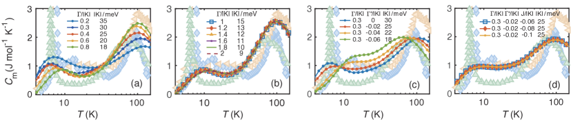
Supplementary Figure 1: Simulations of the magnetic specific heat $C_{\rm m}$. (a,b) show the $C_{\rm m}$ curves with different $\Gamma$ terms, with rest interactions temporarily set to be zero. (c) shows the simulated $C_{\rm m}$ with various $\Gamma^{\prime}$ couplings and fixed $\Gamma/|K|=0.3$, and (d) checks the effects of Heisenberg term $J$ with fixed $\Gamma=0.3$ and $\Gamma^{\prime}=-0.02$. All those curves are compared with experimental data Kubota et al. (2015); Do et al. (2017); Widmann et al. (2019), which are shown in the background. The energy scale $|K|$ is tuned adaptively in different cases to fit the $C_{\rm m}$ curves.

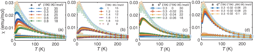
Supplementary Figure 2: Simulations of the magnetic susceptibility $\chi_{\rm ab}$ and $\chi_{\rm c^{*}}$. (a,b) The susceptibility results, including the in-plane susceptibility $\chi_{\rm ab}$ computed under fields $H_{[11\bar{2}]}\parallel\textbf{a}$ and the out-of-plane one $\chi_{\rm c^{*}}$ under $H_{[111]}\parallel\textbf{c}^{*}$, are shown with different $\Gamma/|K|$ values. (c) shows the fittings with various $\Gamma^{\prime}$ and a fixed $\Gamma=0.3$, and (d) the various Heisenberg $J$ with fixed $\Gamma=0.3$ and $\Gamma^{\prime}=-0.02$. The two $g$-factors, i.e., $g_{\rm ab}$ and $g_{\rm c^{*}}$, are determined to be between 2.2-2.5 (depending on other coupling parameters) from fitting the high-temperature susceptibility. The magnetic field $\mu_{0}H$ involved in our fittings are between 0.8-1 T, in consistent with the experimental field of 1 T.

To be concrete, we show in Supplementary Figs. 1, 2 part of our simulated data in the thermodynamic properties. In Supplementary Fig. 1(a,b), we start with scanning over various $\Gamma$ values with ferromagnetic $K<0$, by setting $\Gamma^{\prime}=J=0$ at first. As shown in Supplementary Fig. 1(a), the $C_{\rm{m}}$ curves are sensitive to $\Gamma$ for $\Gamma<1$, while the curves do not change much for $\Gamma\geq 1$ in Supplementary Fig. 1(b), given that the energy scale $|K|$ is properly tuned. Therefore, to uniquely pinpoint the parameter $\Gamma/|K|$, we need to include more thermodynamic measurements like the magnetic susceptibility.

As shown in Supplementary Fig. 2(a,b), as the $\Gamma$ interaction increases, the height of computed susceptibility peak decreases accordingly and deviates the experimental in-plane susceptibility $\chi_{\rm ab}$ curves. After a thorough scanning, we find $\Gamma=0.3$ constitutes an overall optimal parameter in our model fittings of the specific heat and susceptibility. With the given $\Gamma$, we find in Supplementary Fig. 2(c) the susceptibility curves turn out to be not very sensitive to the small $\Gamma^{\prime}$ interactions, while, on the other hand, the low-$T$ peak of $C_{\rm m}$ moves towards higher temperatures as $|\Gamma^{\prime}|$ increases in Supplementary Fig. 1(c). This can be understood as the $\Gamma^{\prime}$ term is crucial for stabilizing the zigzag order when $K<0$ and thus has strong influences on the low-$T$ peak. Therefore, we fix $\Gamma^{\prime}=-0.02$ from the specific heat fittings.

Lastly, we determine the nearest-neighboring Heisenberg term $J$. In Supplementary Fig. 2(d), we find the height of the susceptibility $\chi_{\rm ab}$ peak enhances and thus approaches the experimental curves as $J$ changes from $-0.06$ to $-0.1$, while the specific heat $C_{\rm m}$ is not sensitive to $J$, as shown in Supplementary Fig. 1(d). From these careful scanings in the parameter space, we determine the parameter set as $[\Gamma/|K|,\Gamma^{\prime}/|K|,J/|K|,g_{\rm ab},g_{\rm c^{*}}]=[0.3,-0.02,-0.1,2.5,2.3]$ with $K=-25$ meV, which can very well fit both the specific heat as well as the in- and out-of-plane magnetic susceptibilities.

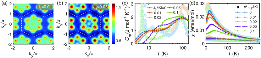
Supplementary Figure 3: Effects of the $J_{3}$ coupling in magnetic structure and thermodynamics. (a,b) show the static spin structure factors of our $\alpha$-RuCl₃ model ($\Gamma/|K|=0.3$, $\Gamma^{\prime}/|K|=-0.02$, $J/|K|=-0.1$) with additional $J_{3}=$ 0.01 and 0.05, respectively. The results are computed at $T\simeq 2.7$ K, and the increased M-point intensity with $J_{3}$ shows that the latter enhances the zigzag order. (c) shows the specific heat $C_{\rm{m}}$ results with various $J_{3}>0$ interactions, as compared to the experimental data in the background. (d) The in- and out-of-plane susceptibility results of our $\alpha$-RuCl₃ model with additional $J_{3}$ values.

The third-nearest neighboring $J_{3}$ interaction. Besides the parameter set considered above, a third neighboring Heisenberg interaction $J_{3}$ has also been suggested to stabilize the zigzag order for $K<0$ Winter et al. (2017, 2017, 2018), which can play a similar role to the off-diagonal $\Gamma^{\prime}$ interaction. In order to explore its effects, we introduce an additional $J_{3}$ term to our $\alpha$-RuCl₃ model and show the computed results in Supplementary Fig. 3.

In the spin structure factors in Supplementary Fig. 3(a,b), we find the M-point intensity clearly enhances when $J_{3}$ increases from 0.01 to 0.05. At the same time, even a small $J_{3}$ can have a considerable impact on the low-temperature thermodynamics and makes our model fittings deviate from the experimental data. In Supplementary Fig. 3(c,d), we find a $J_{3}\geq 0.05$ clearly spoils the fittings to $C_{\rm m}$ and $\chi$: The low-$T$ specific heat peak moves towards higher temperature, and the height of the susceptibility peak gets reduced when increasing $J_{3}$. In addition, from Supplementary Fig. 3(b), $J_{3}=0.05$ interaction evidently cripples the spin intensity at the $\Gamma$ point of the Brillouin zone (BZ). Overall, we find $J_{3}$ indeed plays a very similar role as $\Gamma^{\prime}$ in stabilizing the zigzag order, and, such a term, if exists, should have a small coupling strength. We therefore leave out $J_{3}$ in the main text as well as the discussion below, and mostly focus on the minimal $K$-$J$-$\Gamma$-$\Gamma^{\prime}$ effective model in the main text.

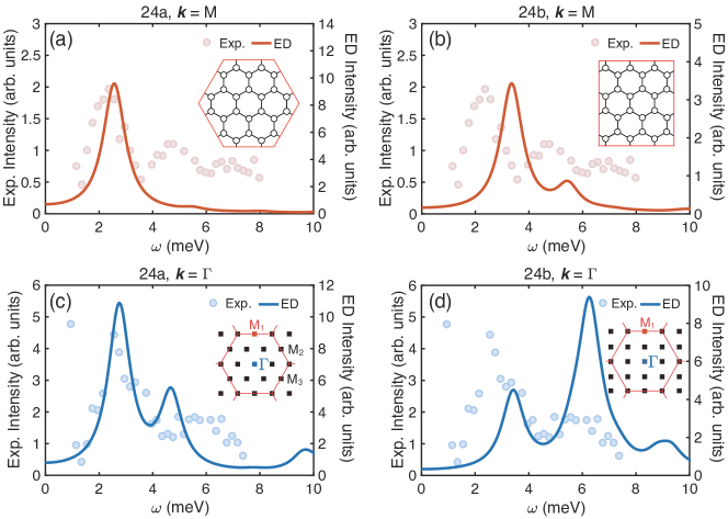
Supplementary Figure 4: The dynamical ED results of intensity $\mathcal{I}(\textbf{k},\omega)$ at the K and $\Gamma$ points. (a,b) shows the constant k-cut of $\mathcal{I}(\textbf{k},\omega)$ at k = M and (c,d) at k = $\Gamma$ points. The dynamical data in (a,c) are computed on cluster 24a with its real-space and reciprocal lattices illustrated in panels (a) and (c), respectively. The corresponding results of 24b cluster are shown in (b,d), note there are no M₂ and M₃ points in the BZ of 24b cluster as illustrated in the inset of (d). The intensity peak locations $\omega_{\rm M}$ and $\omega_{\Gamma}$ are stable [$\omega_{\rm M}$ = 2.5 and 3.3 meV in (a,b), and $\omega_{\Gamma}$ = 2.7 and 3.4 meV in (c,d), respectively] while the relative intensities between two peaks are found more sensitive to the specific geometries due to the finite-size effects.

Exact diagonalization results of dynamical spin structure factors. In the dynamical simulations, the 24-site cluster with $C_{3}$ symmetry (denoted as 24a henceforth) has been widely adopted in ED calculations of the Kitaev model (see, e.g., Refs. Winter et al. (2017); Gordon et al. (2019); Hickey and Trebst (2019); Laurell and Okamoto (2020)). Amongst other geometries that are accessible by ED, the 24a cluster is unique as it contains all the high-symmetry points in the BZ [c.f., inset in Supplementary Fig. 4(c)], which is important for dynamical property calculations. Therefore, we choose the 24a cluster in presenting our dynamical data in the main text. Nevertheless, in Supplementary Fig. 4 we also perform dynamical ED simulations on a different 24-site geometry (24b) and compare the results to those of the 24a cluster. It can be seen in Supplementary Fig. 4 that the positions $\omega_{\rm M}$ and $\omega_{\Gamma}$ of the intensity peaks as well as the double-peak structure of $\Gamma$-intensity curves are qualitatively consistent. Note the 24b cluster shown in Supplementary Fig. 4(b,d) are not $C_{3}$ symmetric and thus does not possess all high symmetry moment points.

Magnetic anisotropy and the off-diagonal $\Gamma$ term. The off-diagonal $\Gamma$ interaction has been suggested to be responsible for the strong magnetic anisotropy between in- and out-of-plane directions Lampen-Kelley et al. (2018); Sears et al. (2020). In a pure Kitaev model without the $\Gamma$ term, it has been shown that the in-plane ($\chi_{\rm ab}$) and out-of-plane ($\chi_{\rm c^{*}}$) susceptibilities are of similar magnitudes Li et al. (2020). On the other hand, as shown in Supplementary Fig. 2, when the $\Gamma$ term is introduced, we find the two susceptibility curves are clearly separated, suggesting that the off-diagonal $\Gamma$ interaction indeed constitutes a resource of strong easy-plane anisotropy observed in $\alpha$-RuCl₃.

Automatic searching of the Hamiltonian parameters. Through the fitting process described above, we have manually determined an accurate set of model parameters of $\alpha$-RuCl₃. As a double-check, below we exploit the recently developed automatic parameter searching technique based on the Bayesian approach Yu et al. to conduct a global optimization of the model parameters in Supplementary Fig. 5. The target is to minimize the fitting loss of the simulated results to measured thermodynamic quantities, including the specific heat $C_{\rm m}$ as well as the in- ($\chi_{\rm ab}$) and out-of-plane ($\chi_{\rm c^{*}}$) susceptibilities. Since the specific heat data vary greatly in various measurements and the lower-$T$ peak diverges likely due to 3D effects, we take the mean values of several measurements as the specific heat data $C_{\rm m}^{\rm exp}(T)$ used in the fittings. In practice, the loss function $\mathcal{L}$ is designed as follows:

$$\begin{split}\mathcal{L}=\text{log}\{\frac{\lambda_{\chi}}{N_{\chi_{\rm ab}}}\sum_{T>T_{\rm cut}}[{\chi_{\rm ab}^{\rm exp}(T)-\chi_{\rm ab}^{\rm sim}(T)}]^{2}&+\frac{\lambda_{\chi}}{N_{\chi_{\rm c^{*}}}}\sum_{T>T_{\rm cut}}[{\chi_{\rm c^{*}}^{\rm exp}(T)-\chi_{\rm c^{*}}^{\rm sim}(T)}]^{2}\\ &+\frac{\mathcal{P}\,\lambda_{C}}{N_{C_{\rm m}}}\sum_{T>T^{\prime}_{\rm cut}}[{C_{\rm m}^{\rm exp}(T)-C_{\rm m}^{\rm sim}(T)}]^{2}\},\end{split}$$ (S1)

where $\lambda_{C}=1/{\mathrm{max}(C_{\rm m}^{\rm exp})}^{2}$ and $\lambda_{\chi}=1/{\mathrm{max}(\chi_{ab}^{\rm exp})}^{2}$ controls the weights of specific heat and magnetic susceptibility in defining the fitting loss function. $N_{\chi_{\rm ab}}$, $N_{\chi_{\rm c^{*}}}$, and $N_{C_{\rm m}}$ are the data point numbers in three experimental curves, respectively. To focus on the fittings of the locations of two specific heat peaks at 100 K and 8 K, respectively, we further introduce a penalty factor $\mathcal{P}$ defined as

$$\mathcal{P}=\left\{\begin{matrix}\text{min}[\frac{1}{2}\sum_{i}^{1,2}\text{exp}({\frac{|T_{i}^{\rm exp}-T_{i}^{\rm sim}|}{0.15\,T_{i}^{\rm exp}}})-1,a]+\text{min}[\frac{1}{2}\sum_{i}^{1,2}\text{exp}({\frac{|C_{i}^{\rm exp}-C_{i}^{\rm sim}|}{0.25\,C_{i}^{\rm exp}}})-1,a]&,&\text{ two peaks}\\ 2a&,&\text{otherwise}\end{matrix}\right.$$ (S2)

where $\{T_{1},T_{2}\}=\{100~{}\text{K},8~{}\text{K}\}$ are the position of the peaks, with $\{C_{1},C_{2}\}$ the specific heat value at corresponding higher and lower $T$. As our many-body calculations are performed on a finite-size system, we need to introduce the $T_{\rm cut}(T^{\prime}_{\rm cut})$ as the lowest temperature involved in the fittings, and in practice it is set as $T_{\rm cut}=25$ K for magnetic susceptibility and $T^{\prime}_{\rm cut}=3$ K for the specific heat data. The factor $\mathcal{P}$ emphasizes the double-peak structure as well as the locations and heights of each peaks in the simulated $C_{\rm m}$, where we set an empirical factor $a=2$ to enlarge the loss function as a penalty for the simulated specific heat curves without double-peak structure.

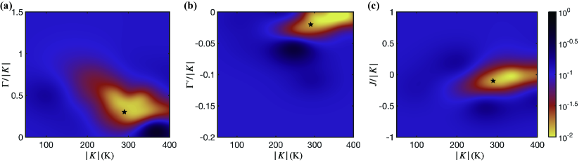
Supplementary Figure 5: The estimated fitting loss $\mathcal{L}$ shown in (a) $K$-$\Gamma$, (b) $K$-$\Gamma^{\prime}$, and (c) $K$-$J$ planes. The results are obtained by Bayesian optimization through 120 iterations of XTRG calculations on the YC4$\times$4$\times$2 cylinder. The asterisk represents the optimal parameter set found to also reproduce other major experimental observations including the magnetization curve and dynamical spin structures, which is located within the bright regime with small fitting loss of thermodynamics. The two Landé factors $g_{\rm ab}$ and $g_{\rm c^{*}}$ at each parameter point are tuned to their optimal values (between 1.5 and 3) to minimize the loss $\mathcal{L}$. Note, when plotting the cross sectors, like the $K$-$\Gamma$ plane in (a), the other model parameters are fixed at their optimal values.

In Supplementary Fig. 5, we show the estimated loss $\mathcal{L}$ in the $K$-$\Gamma$, $K$-$\Gamma^{\prime}$, and $K$-$J$ planes, respectively. From the color map of $\mathcal{L}$, we see clearly optimal (bright) regimes, and the determined optimal parameter set in the main text is indicated by the asterisk, i.e., $K=-25$ meV, $\Gamma=0.3\ |K|$, $\Gamma^{\prime}=-0.02\ |K|$, and $J=-0.1\ |K|$, with the in- and out-of-plane Landé factors found to be $g_{\rm ab}=2.5$ and $g_{\rm c^{*}}=2.3$, respectively, which can fit excellently both the thermodynamic and dynamic measurements in Fig. 2 of the main text.

Supplementary Note 2 Revisit of Various $\alpha$-RuCl₃ Candidate Models

We now employ XTRG to revisit some of the previously proposed $\alpha$-RuCl₃ candidate models in the literature Winter et al. (2016, 2017); Wu et al. (2018); Cookmeyer and Moore (2018); Kim and Kee (2016); Suzuki and Suga (2019); Ran et al. (2017); Wang et al. (2017b); Ozel et al. (2019), where the Kitaev coupling $K$, Heisenberg $J$ (nearest neighboring), $J_{3}$ (third-nearest neighboring), as well as off-diagonal $\Gamma$ and $\Gamma^{\prime}$ terms are considered. We calculated the thermodynamics and static spin structure factors, the main results are summarized in Supplementary Table. 1 and the detailed thermodynamic results are shown in Supplementary Figs. 6 and 7.

Refs.	$K$ (meV)	$\Gamma/|K|$	$\Gamma^{\prime}/|K|$	$J/|K|$	$J_{3}/|K|$	${C_{\rm{m}}}^{{\dagger}}$	$\chi_{a}$	$\chi_{\rm c^{*}}$	zigzag order‡	M-star ∗
Winter2016 Winter et al. (2016)	-6.7	0.985	-0.134	-0.254	0.403	✗	✗	✓	✓	✗
Winter2017 Winter et al. (2017)	-5	0.5	/	-0.1	0.1	✗	✗	✗	✓	✗
Wu2018 Wu et al. (2018)	-2.8	0.857	/	-0.125	0.121	✗	✗	✗	✓	✗
Cookmeyer2018 Cookmeyer and Moore (2018)	-5	0.5	/	-0.1	0.023	✗	✗	✗	✓	✓
Kim2016 Kim and Kee (2016)	-6.55	0.802	-0.145	-0.234	/	✗	✓	✓	✓	✗
Suzuki2019 Suzuki and Suga (2019)	-24.4	0.215	-0.039	-0.063	/	✓	✓	✓	✓	✗
Ran2017 Ran et al. (2017)	-6.8	1.397	/	/	/	✓	✓	✓	✗	✓
Wang2017 Wang et al. (2017b)	-10.9	0.56	/	-0.028	0.003	✗	✓	✓	✗	✗
Ozel2019 Ozel et al. (2019)	-3.5	0.671	/	0.131	/	✗	✗	✗	✗	✗
Our model⋆	-25	0.3	-0.02	-0.1	/	✓	✓	✓	✓	✓
${{\dagger}}$ Check if the double-peak feature exists in the calculated $C_{\rm{m}}$ curves.
${\ddagger}$ Check if the model exhibits a low-$T$ zigzag order.
$\ast$ Check if the dynamical M-star structure exists (taken from Ref. Laurell and Okamoto (2020), except for our model in the last row).
$\star$ Our $\alpha$-RuCl3 model proposed in the main text.

Supplementary Table 1: Checklist of various candidate models of $\alpha$-RuCl₃ on typical experimental features. The “✓ ” symbol indicates a good fitting between model calculations and experimental measurements, while “✗ ” represents a disagreement between the two.

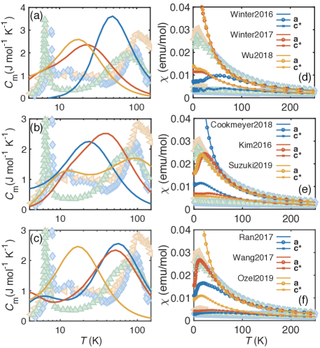
Supplementary Figure 6: Thermodynamic properties of various $\alpha$-RuCl₃ candidate models. (a-c) The magnetic specific heat $C_{\rm m}$ curves (marked as solid lines) compared to the experimental measurements. (d-f) The susceptibility data with fields $\mu_{0}H\parallel$ a and c^∗ around 1 T. The calculations are performed on YC4$\times$4$\times$2 lattice.

Specific heat and susceptibility curves. In Supplementary Fig. 6 we show the simulated magnetic specific heat $C_{\rm m}$ and susceptibility $\chi$ of various candidate models, and compare them to the experimental measurements. From Supplementary Fig. 6(a-c), we find only the models Suzuki2019 Suzuki and Suga (2019) and Ran2017 Ran et al. (2017) exhibit a double-peaked $C_{\rm m}$ curve, each located at the characteristic temperature precisely as in experiments. For the rest of revisited candidate models, however, we did not observe the desired double-peak feature in the right temperature window.

The magnetic susceptibility results of the candidate models are shown in Supplementary Fig. 6(d-f), where we find four models out of them, i.e., Kim2016 Kim and Kee (2016), Suzuki2019 Suzuki and Suga (2019), Ran2017 Ran et al. (2017), and Wang2017 Wang et al. (2017b) offer adequate fittings to both in- and out-of-plane susceptibility measurements, with similar Landé factors $g_{\rm ab}$ and $g_{\rm c^{*}}$ ranging between 2.1 and 2.3 (depending on the specific candidate model).

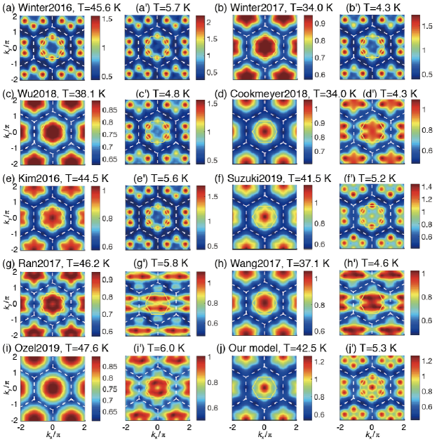
Supplementary Figure 7: Color maps of the static spin structure factors $S(\textbf{k})$ of various candidate $\alpha$-RuCl₃ models. (a-j) show the intermediate-$T$ results and (a^′-j^′) show their low-$T$ counterparts.

Spin structures and the low-$T$ zigzag order. The compound $\alpha$-RuCl₃ exhibits a zigzag antiferromagnetic order below $T\simeq 7$ K Kubota et al. (2015); Do et al. (2017); Widmann et al. (2019); Sears et al. (2015); Banerjee et al. (2017), which corresponds to a spin structure peak at the M point. Therefore, in Supplementary Fig. 7 we show the static spin structure factors $S(\textbf{k})=\sum_{\gamma=\{x,y,z\}}S^{\gamma\gamma}(\textbf{k})$ at an intermediate $T\sim 40$ K [see Supplementary Fig. 7(a-j)] and a low temperature $T\sim 5$ K [Supplementary Fig. 7(a^′-j^′)]. Besides the prominent M-peak at low $T$, we also anticipate a M-star static structure factor emerging at intermediate temperatures, which reflects the short-range spin correlations at both the $\Gamma$ and M points of the BZ. All these features can be well reproduced in the candidate models Winter2017 Winter et al. (2017), Wu2018 Wu et al. (2018), Cookmeyer2018 Cookmeyer and Moore (2018), Kim2016 Kim and Kee (2016), and Suzuki2019 Suzuki and Suga (2019). As for the dynamical structure factors, it has been discussed before in Ref. Laurell and Okamoto (2020) that only the models Cookmeyer2018 Cookmeyer and Moore (2018) and Ran2017 Ran et al. (2017) could reproduce the M-star shape of the inelastic neutron scattering intensity, when integrated over [4.5, 7.5] meV Banerjee et al. (2018).

Overall, as concluded in Ref. Laurell and Okamoto (2020), we also find no single candidate model revisited here can satisfactorily explain all observed phenomena of experiments on $\alpha$-RuCl₃. For example, both Cookmeyer2018 Cookmeyer and Moore (2018) and Ran2017 Ran et al. (2017) have M-star shape in the intermediate-energy dynamical spin structure, however, the former does not fit the specific heat and susceptibility measurements well and the latter does not host a zigzag oder at low temperature. Nevertheless, we note that the model Suzuki2019 Suzuki and Suga (2019) can reproduce the prominent thermodynamic features such as the double-peaked specific heat, highly anisotropic susceptibility, and zigzag static spin structures (although the dynamical M star was not found in this candidate model according to Ref. Laurell and Okamoto (2020)). Our model, on the other hand, accurately describes the spin interactions and explain thus major experimental findings in the compound $\alpha$-RuCl₃.

Supplementary Note 3 $\alpha$-RuCl₃ Model Simulations under In-plane and Tilted Magnetic Fields

In this Note, we show various thermodynamic properties of $\alpha$-RuCl₃ under in-plane and tilted $\textbf{c}^{\prime}$ fields (see Fig. 1b in the main text), and compare the simulated results to experimental measurements.

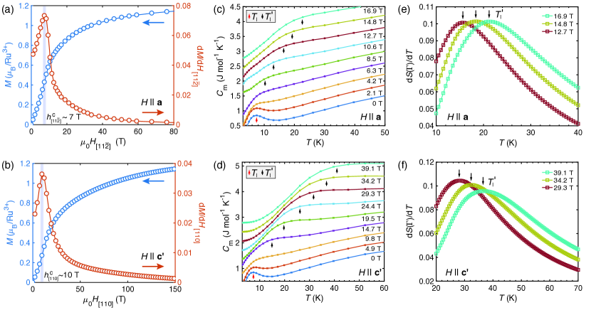
Supplementary Figure 8: Magnetization curves and thermodynamic properties under fields $H_{[11\bar{2}]}\parallel\textbf{a}$ and $H_{[110]}\parallel\textbf{c}^{\prime}$. The ground-state magnetization curves, under (a) in-plane field $H_{[11\bar{2}]}$ along a- and (b) the tilted $H_{[110]}$ along $\textbf{c}^{\prime}$-axis, are plotted with their derivatives $dM/dH$, where only one QPT can be observed in both cases. (c, d) Low-temperature specific heat curves $C_{\rm m}$, with each curve shifted by 0.35 J mol^-1 K^-1 vertically for clarify. The low-$T$ scale $T_{\rm l}$ and $T_{\rm l}^{\prime}$ are indicated by the red and black arrows, respectively. (e,f) show the temperature derivatives of the uniform magnetization, i.e., $dS(\Gamma)/dT$, with the peaks located at $T^{\prime}_{\rm l}$.

Magnetization curves along the a- and $\textbf{c}^{\prime}$-axis. In Supplementary Fig. 8(a,b), we show the magnetization curves obtained from the $T=0$ DMRG calculations on YC4$\times$4$\times$2 geometry. QPT takes place at 7 T and 10 T, for $H_{[11\bar{2}]}\parallel\textbf{a}$ and $H_{[110]}\parallel\textbf{c}^{\prime}$, respectively. The QPT is clearly signaled by the divergent derivative $dM/dH$, where the zigzag order becomes suppressed and the system enters the polarized phase. As the field further increases, the uniform magnetization $M$ gradually approaches the saturation value.

Specific heat under magetic fields and the Zeeman energy scale $T^{\prime}_{\rm l}$. In Supplementary Fig. 8(c,d), we show the low-$T$ part of the magnetic specific heat curves on YC4$\times$6$\times$2 systems calculated by XTRG. For $\mu_{0}H_{[11\bar{2}]}<7$ T, we find the height of the $C_{\rm m}$ peaks is suppressed by fields, and the low-temperature scale $T_{\rm l}$ associated with the zigzag order, as indicated by the red arrow in Supplementary Fig. 8(c), decreases to zero when the field approaches the critical value, in agreement with experiments Kubota et al. (2015). Above that, a new low-temperature scale $T^{\prime}_{\rm l}$ builds up and moves towards higher temperatures almost linearly vs $H_{[11\bar{2}]}$, as indicated by the black arrows in Supplementary Fig. 8(c). We find $T^{\prime}_{\rm l}$ is intimately related to the uniform magnetization, as observed from the temperature variation of spin structure intensity $S(\Gamma)$. In Supplementary Fig. 8(e), we show the derivative ${\rm d}S(\Gamma)/{\rm d}T$ exhibits clear peaks, whose locations are in agreement with the temperature scale $T^{\prime}_{\rm l}$ determined from the low-temperature peak of $C_{\rm m}$ in Supplementary Fig. 8(c). The peaks moving towards higher temperature as the magnetic field increases, and we thus relate $T^{\prime}_{\rm l}$ to the Zeeman energy scale. Beside in-plane fields, as depicted in Supplementary Fig. 8(d,f), the case of $H_{[110]}\parallel\textbf{c}^{\prime}$ exhibits very similar behaviors.

Energy spectra under in-plane fields. In Supplementary Fig. 9 we show ED results of the energy spectra on the 24-site cluster (24a), under two in-plane fields $H_{[11\bar{2}]}\parallel\textbf{a}$ and $H_{[1\bar{1}0]}\parallel\textbf{b}$ axis [c.f., Supplementary Fig. 9(a)]. The energy spectra results under various fields are plotted in Supplementary Fig. 9(b) and (c), for $H\parallel\textbf{a}$ and b, respectively. From there we observe the spin gap $(E_{\rm 1}-E_{\rm 0})$ changes its behavior at an intermediate field, which can be estimated as the transition field $h_{[11\bar{2}]}^{c}$ and $h_{[1\bar{1}0]}^{c}$, and the spectra appear differently along a and b directions, consistent with the observation in recent experiments Lampen-Kelley et al. (2018); Yokoi et al. .

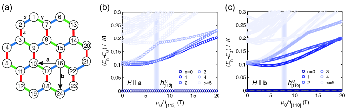
Supplementary Figure 9: The energy spectra under in-plane magnetic fields. (a) The 24-site cluster involved in the ED calculations, with the directions of two in-plane fields $H_{[11\bar{2}]}\parallel\textbf{a}$ and $H_{[1\bar{1}0]}\parallel\textbf{b}$ indicated by the black arrows. (b,c) show the energy spectra ($E_{\rm n}-E_{\rm 0})$ under the in-plane fields, with the ground-state energy $E_{0}$ subtracted. In two cases, the spin gap starts to increase rapidly at about $h_{[11\bar{2}]}^{c}\simeq 7$ T and $h_{[1\bar{1}0]}^{c}\simeq 8$ T, respectively, as indicated by the thick vertical lines.

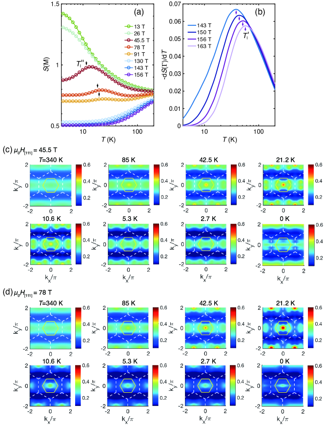
Supplementary Figure 10: The spin structure factors under out-of-plane $H_{[111]}$ fields. We show (a) the $S($M$)$ and (b) $-dS(\Gamma)/dT$ curves with temperature $T$, which are computed on the YC4$\times$6$\times$2 lattice. The black arrows in (a) represent the temperature scale $T^{\prime\prime}_{\rm l}$ determined from the low-$T$ peak of the specific heat in Fig. 6 of the main text, and the purple ones in (b) indicates the low-$T$ scales $T^{\prime}_{\rm l}$ which locates at the peak of $-dS(\Gamma)/dT$. The static spin-structure factors $\tilde{S}^{zz}(\textbf{k})$ [following the definition in Eq. (2) of the main text] under the field of $\mu_{0}H_{[111]}=45.5$ T and 78 T are shown in (c) and (d), respectively, from high to low temperatures and compared to the ground-state results. The data are plotted here in the same colorbar as that in Fig. 3e-g of the main text.

Supplementary Note 4 Quantum Spin Liquid under Out-of-plane Magnetic Fields

Finite-temperature Spin structures under out-of-plane fields. In Supplementary Fig. 10, we plot the spin structure factors at two typical momentum points in the BZ, i.e., $\textbf{k}=$M and $\Gamma$. From the $S({\rm M})$ curves in Supplementary Fig. 10(a), we find the zigzag order [cf. 13 T and 26 T lines in Supplementary Fig. 10(a)] gets suppressed in the quantum spin liquid (QSL) phase under strong out-of-plane magnetic fields [see, e.g., 45.5 T, 78 T, and 91 T lines in Supplementary Fig. 10(a)]. In the QSL phase, there exists enhanced M-point spin correlation near the emergent lower temperature scale $T^{\prime\prime}_{\rm l}$, as indicated by the black arrows in Supplementary Fig. 10(a). In Supplementary Fig. 10(b), we show the temperature derivative $-dS(\Gamma)/dT$, whose peak position signals the low-temperature scale $T^{\prime}_{\rm l}$, below which the field-induced uniform magnetization gets established, i.e., $T^{\prime}_{\rm l}$ is a crossover temperature scale to the polarized state. As shown in Supplementary Fig. 10(b), $T^{\prime}_{\rm l}$ moves to higher temperatures as the field increases.

In the main text, we have discussed the static spin-structure factors $\tilde{S}^{zz}(\textbf{k})$ under an out-of-plane field of 45.5 T (cf. the insets of Fig. 5b of the main text). In Supplementary Fig. 10(c,d), we supplement with XTRG results of $\tilde{S}^{zz}(\textbf{k})$ at various temperatures and under two fields, 45.5 T and 78 T. For each case, we compare the finite-$T$ XTRG results to the $T=0$ data obtained by DMRG. At high temperature, i.e., $T=340$ K, the spin structure is virtually featureless for both cases, with only a faint stripe due to the strong Kitaev interaction ($\sim-25$ meV), which becomes more and more clear as the system cools down near the low-$T$ scale $T^{\prime\prime}_{\rm l}$, around which the brightness at $\Gamma$ and M points are slightly enhanced due to the strong spin fluctuations. When $T<T^{\prime\prime}_{\rm l}$ the $\Gamma$ peak in the spin structures becomes flattened, yet the stripy background remains distinct, which is in excellent agreement with the DMRG results, supporting strongly the existence of QSL state under high out-of-plane fields.

Ground-state static spin structures under a field of 78 T. In Supplementary Fig. 11 and Supplementary Fig. 12, we show the ground-state static structure factor $\tilde{S}^{\alpha\beta}(\textbf{k})={\sum_{j\in{\rm bulk},\ j\neq i_{0}}}e^{i\textbf{k}\cdot(\textbf{r}_{j}-\textbf{r}_{i_{0}})}(\langle S^{\alpha}_{i_{0}}S^{\beta}_{j}\rangle-\langle S^{\alpha}_{i_{0}}\rangle\langle S^{\beta}_{j}\rangle)$ of our $\alpha$-RuCl₃ model on cylinders of different sizes in the high-field QSL phase (under a magnetic fields of 78 T), obtained by DMRG simulations with bond dimension up to $D=2048$. Here we fix a central site $i_{0}$ and compute the correlations with respect to this reference site, instead of computing the all-to-all correlations, to speed up the computations. From Supplementary Fig. 11, we find strong stripy background in $\tilde{S}^{xx}$, $\tilde{S}^{yy}$, and $\tilde{S}^{zz}$, divided by $N_{\rm{bulk}}$, where $N_{\rm{bulk}}$ is the number of bulk sites (i.e., with the left- and right-most columns of the cylinder skipped), representing intrinsic Kitaev spin liquid characteristics. There also exists a bright $\Gamma$ point in the BZ, and we depict the profiles with fixed $k_{y}=0$ in Supplementary Fig. 12, to check whether the structure factor diverges at any k point. In Supplementary Fig. 12 we find both the diagonal part $\tilde{S}_{{\rm diag}}(\textbf{k})=\sum_{\alpha,\beta}{\tilde{S}^{\alpha\beta}(\textbf{k})\delta_{\alpha\beta}}$ and the off-diagonal part $\tilde{S}_{{\rm off-diag}}(\textbf{k})=\sum_{\alpha,\beta}{\tilde{S}^{\alpha\beta}(\textbf{k})(1-\delta_{\alpha\beta})}$, when divided by $N_{\rm bulk}$, are moving towards zero as the system size increases, indicating the absence of spontaneous long-range order in the phase.

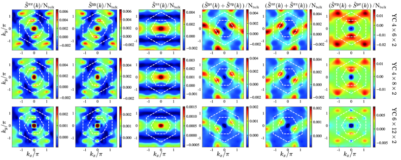
Supplementary Figure 11: Color maps of the static spin structure factors $\tilde{S}^{\alpha\beta}(\textbf{k})/{N_{\rm{bulk}}}$. The results are calculated in the intermediate QSL phase under $\mu_{0}H_{[111]}\simeq 78$ T on cylinders of different sizes, obtained by DMRG simulations.

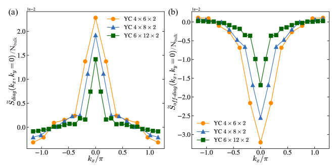
Supplementary Figure 12: The static spin structure factors cut at $k_{y}=0$. (a) shows $\tilde{S}_{\rm diag}(k_{x},k_{y}=0)/{N_{\rm{bulk}}}$ and (b) $\tilde{S}_{\rm off-diag}(k_{x},k_{y}=0)/{N_{\rm{bulk}}}$ in the intermediate QSL phase under $\mu_{0}H_{[111]}\simeq 78$ T on cylinders of different sizes.

Ground-state entanglement scaling. The nature of the intermediate QSL phase can be further characterized by entanglement scaling in the ground state. Here we study the von Neumann entanglement entropy $S_{v}$. Considering a bipartition of the system into two parts A and B, the reduced density matrix of A can be obtained by tracing out the degrees of freedom of B, i.e., $\rm\rho_{A}=Tr_{B}\rho$, where $\rho=|\psi_{0}\rangle\langle\psi_{0}|$ is density matrix of the normalized ground state $|\psi_{0}\rangle$ of the whole system. The von Neumann entropy is defined as

$$S_{v}=-\rm{Tr}(\rho_{A}ln\rho_{A}).$$ (S3)

Here, we consider the cut along circumference direction and measure $S_{v}$ for each cut at $l$. By virtue of the conformal mapping: $l\rightarrow\tilde{l}=(L/\pi)\sin(\pi l/L)$, a central charge $c$ on the open cylindrical geometry can be formally extracted using

$$S_{v}=\frac{c}{6}\ln{\tilde{l}}+{\rm const.},$$ (S4)

originally proposed in the (1+1)-D conformal field theory. The prominent “dome”-like $S_{v}$ curves in Supplementary Fig. 13(a) together with the linear fitting with effective central charge $c$ in Supplementary Fig. 13(b), indicates a gapless intermediate phase. This is consistent with the gapless feature observed in the energy spectra as shown in Fig. 5d and algebraic magnetic specific heat in Fig. 6d of the main text. Furthermore, the effective central charge $c$ increases with the system width $W$, i.e. the allowed $\hat{y}$ momenta in the Brillouin zone, suggesting the increased gapless modes.

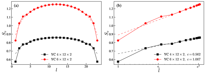
Supplementary Figure 13: The ground-state entanglement entropy $S_{v}$ in the intermediate phase. (a) The $S_{v}$ profile over the system with $\mu_{0}H_{[111]}\simeq 78$ T on cylinders of length $L=12$. (b) $S_{v}$ versus conformal distance $\tilde{l}\equiv(L/\pi)\sin(\pi l/L)$ in logarithmic scale. The fittings are plotted as dashed lines in both panels, which reveal a central charge $c$ close to 0.5 and 1 for $W=4$ and 6, respectively.

Supplementary Note 5 Variational Monte Carlo Results

Spin-liquid ansatz based on $D_{\rm 3d}\times Z_{2}^{T}$ symmetry. We start with the extended Kitaev honeycomb model containing $K$, $J$, $\Gamma$ and $\Gamma^{\prime}$ interactions. The most general expression of the mean-field Hamiltonian ansatz Wang et al. (2019, 2020); Liu and Normand (2018) with nearest-neighbor couplings reads

$$H_{\rm mf}^{\rm SL} = \!\!\!\!\sum_{\langle i,j\rangle\in\alpha\beta(\gamma)}\!\!\!\Big{(}{\rm Tr}\,[U_{ji}^{(0)}\psi_{i}^{\dagger}\psi_{j}]\!+\!{\rm Tr}\,[U_{ji}^{(1)}\psi_{i}^{\dagger}(iR_{\alpha\beta}^{\gamma})\psi_{j}]+{\rm Tr}\,[U_{ji}^{(2)}\psi_{i}^{\dagger}\sigma^{\gamma}\psi_{j}]\!+\!{\rm Tr}\,[U_{ji}^{(3)}\psi_{i}^{\dagger}\sigma^{\gamma}R_{\alpha\beta}^{\gamma}\psi_{j}]\!+\!{\rm H.c.}\Big{)}$$ (S5)

$$\;\;\;\;+\sum_{i}{\rm Tr}(\boldsymbol{\lambda}_{i}\cdot\psi_{i}\boldsymbol{\tau}\psi_{i}^{\dagger}),$$

where $\psi_{i}=(C_{i}\ \bar{C}_{i})$, $C_{i}=(c_{i\downarrow},c_{i\uparrow})^{T},\bar{C}_{i}=(c_{i\downarrow}^{\dagger},-c_{i\uparrow}^{\dagger})^{T}$, and $R_{\alpha\beta}^{\gamma}=-\frac{i}{\sqrt{2}}(\sigma^{\alpha}+\sigma^{\beta})$. Owing to the subtle $SU(2)$ gauge symmetry Affleck et al. (1988) in the fermionic spinon representation, the particle number constraint $\hat{N}_{i}=1$ is extended into the $SU(2)$ gauge invariant three-component form ${\rm Tr}(\boldsymbol{\psi}_{i}\boldsymbol{\tau}\psi_{i}^{\dagger})=0$ which are ensured by the three Lagrangian multipliers $\lambda^{x,y,z}$, where $\tau^{x,y,z}$ are the generators of the $SU(2)$ gauge group. The matrices $U_{ji}^{(0,1,2,3)}$ can be expanded with the identity matrix and $\tau^{x,y,z}$, where the expanding coefficients form a subset of $\boldsymbol{R}$. For the present model, the $SU(2)$ gauge symmetry breaks down to its subgroup $Z_{2}$ (which is called the invariant gauge group, IGG) and the resultant quantum spin liquids are $Z_{2}$ QSLs.

A QSL ground state preserves the whole space group symmetry whose point group is $D_{\rm 3d}\times Z_{2}^{T}$. However, the symmetry group of a spin liquid mean-field Hamiltonian is the projective symmetry group (PSG) Wen (2002); You et al. (2012) whose group elements are space group operations followed by $SU(2)$ gauge transformations. Although there are more than 100 classes of PSGs for Z₂ QSLs, here we adopt the PSG that describes the symmetry of the mean-field Hamiltonian of the pure Kitaev model (called Kitaev PSG). Under this constraint, the allowed mean-field Hamiltonian contains the following parameters.

Firstly, recalling that in KSL the Kitaev interactions are decoupled in a way that the $c$ Majorana fermions are not mixed with the $b^{\gamma}$ Majorana fermions, we have

$$H_{\rm mf}^{K} = \sum_{\langle i,j\rangle\in\alpha\beta(\gamma)}\rho_{a}(ic_{i}c_{j})+\rho_{c}(ib_{i}^{\gamma}b_{j}^{\gamma})$$

$$= \sum_{\langle i,j\rangle\in\alpha\beta(\gamma)}\Big{(}i\rho_{a}{\rm Tr}\big{(}\psi_{i}^{\dagger}\psi_{j}+\tau^{x}\psi_{i}^{\dagger}\sigma^{x}\psi_{j}+\tau^{y}\psi_{i}^{\dagger}\sigma^{y}\psi_{j}+\tau^{z}\psi_{i}^{\dagger}\sigma^{z}\psi_{j}\big{)}$$

$$+i\rho_{c}{\rm Tr}\big{(}\psi_{i}^{\dagger}\psi_{j}+\tau^{\gamma}\psi_{i}^{\dagger}\sigma^{\gamma}\psi_{j}-\tau^{\alpha}\psi_{i}^{\dagger}\sigma^{\alpha}\psi_{j}-\tau^{\beta}\psi_{i}^{\dagger}\sigma^{\beta}\psi_{j}\big{)}+{\rm H.c.}\Big{)}$$

Similarly, the $\Gamma$ interactions are decoupled as

$$H_{\rm mf}^{\Gamma} = \!\!\sum_{\langle i,j\rangle\in\alpha\beta(\gamma)}\!\!i\rho_{d}(b_{i}^{\alpha}b_{j}^{\beta}+b_{i}^{\beta}b_{j}^{\alpha})$$

$$= \!\!\sum_{\langle i,j\rangle\in\alpha\beta(\gamma)}\!\!\Big{(}i\rho_{d}{\rm Tr}\big{(}\tau^{\alpha}\psi_{i}^{\dagger}\sigma^{\beta}\psi_{j}+\tau^{\beta}\psi_{i}^{\dagger}\sigma^{\alpha}\psi_{j}\big{)}+{\rm H.c.}\Big{)},$$

and the $\Gamma^{\prime}$ interactions are decoupled as

$$H_{\rm mf}^{\Gamma^{\prime}} = \!\!\sum_{\langle i,j\rangle\in\alpha\beta(\gamma)}\!\!i\rho_{f}(b_{i}^{\alpha}b_{j}^{\gamma}+b_{i}^{\gamma}b_{j}^{\alpha}+b_{i}^{\beta}b_{j}^{\gamma}+b_{i}^{\gamma}b_{j}^{\beta})$$

$$= \!\!\sum_{\langle i,j\rangle\in\alpha\beta(\gamma)}\!\!\Big{(}i\rho_{f}{\rm Tr}\big{(}\tau^{\alpha}\psi_{i}^{\dagger}\sigma^{\gamma}\psi_{j}+\tau^{\gamma}\psi_{i}^{\dagger}\sigma^{\alpha}\psi_{j}+\tau^{\beta}\psi_{i}^{\dagger}\sigma^{\gamma}\psi_{j}+\tau^{\gamma}\psi_{i}^{\dagger}\sigma^{\beta}\psi_{j}\big{)}+{\rm H.c.}\Big{)}.$$

Comparing with the general form Supplementary Eq. (S5), the decouplings expressed in Supplementary Eqs. (Supplementary Note 5), (Supplementary Note 5) and (Supplementary Note 5) contribute the terms ${\tilde{U}}_{ji}^{(0)}=i(\rho_{a}+\rho_{c}),\ {\tilde{U}}_{ji}^{(1)}=i(\rho_{a}-\rho_{c}+\rho_{d}+2\rho_{f})(\tau^{\alpha}+\tau^{\beta}),\ {\tilde{U}}_{ji}^{(2)}=i(\rho_{a}+\rho_{c})\tau^{\gamma}+i\rho_{f}(\tau^{\alpha}+\tau^{\beta}),\ {\tilde{U}}_{ji}^{(3)}=i(\rho_{c}-\rho_{a}-\rho_{d})(\tau^{\alpha}-\tau^{\beta}),$ to the coefficients $U_{ji}^{(m)}$, in which $j$ and $i$ specify $\gamma$.

Secondly, we consider a more general mean-field decoupling which means $c$ Majorana fermions can mix with $b^{\gamma}$ Majorana fermions. In addition, the most general coefficients preserving the $C_{3}$ rotation symmetry (in the PSG sense) also contain multiples of the uniform ($I$) and $\tau^{x}+\tau^{y}+\tau^{z}$ gauge components, ${\tilde{\tilde{U}}_{ji}^{(0)}}=i\eta_{0}+\eta_{1}(\tau^{x}+\tau^{y}+\tau^{z}),\ {\tilde{\tilde{U}}_{ji}^{(1)}}=\eta_{2}+i\eta_{3}(\tau^{x}+\tau^{y}+\tau^{z}),\ {\tilde{\tilde{U}}_{ji}^{(2)}}=\eta_{4}+i\eta_{5}(\tau^{x}+\tau^{y}+\tau^{z}),\ {\tilde{\tilde{U}}_{ji}^{(3)}}=\eta_{6}+i\eta_{7}(\tau^{x}+\tau^{y}+\tau^{z}).$ If the full symmetry group, $G=D_{\rm 3d}\times Z_{2}^{T}$, is preserved, then only three parameters $\eta_{0}$, $\eta_{3}$, and $\eta_{5}$ are allowed. Thus a spin-liquid ansatz that preserves the full Kitaev PSG contains the variables $U_{ji}^{(m)}={\tilde{U}}_{ji}^{(m)}+{\tilde{\tilde{U}}_{ji}^{(m)}}$, namely

$$U_{ji}^{(0)}=i(\rho_{a}+\rho_{c})+i\eta_{0},$$ (S9)

$$U_{ji}^{(1)}=i(\rho_{a}-\rho_{c}+\rho_{d}+2\rho_{f})(\tau^{\alpha}+\tau^{\beta})+i\eta_{3}(\tau^{x}+\tau^{y}+\tau^{z}),$$

$$U_{ji}^{(2)}=i(\rho_{a}+\rho_{c})\tau^{\gamma}+i\rho_{f}(\tau^{\alpha}+\tau^{\beta})+i\eta_{5}(\tau^{x}+\tau^{y}+\tau^{z}),$$

$$U_{ji}^{(3)}=i(\rho_{c}-\rho_{a}-\rho_{d})(\tau^{\alpha}-\tau^{\beta}),$$

with seven real parameters, $\rho_{a}$, $\rho_{c}$, $\rho_{d}$, $\rho_{f}$, $\eta_{0}$, $\eta_{3}$ and $\eta_{5}$.

Magnetically ordered states. Because fermions do not condense alone to form a magnetic order, we introduce the classical order under single-${\boldsymbol{Q}}$ approximation Rau et al. (2014) to describe the magnetic order of the spin-symmetry-breaking phases of the $K$-$J$-$\Gamma$-$\Gamma^{\prime}$ model.

$$\boldsymbol{M}_{i}=M\{\sin\phi[\hat{\boldsymbol{e}}_{x}\cos(\boldsymbol{Q}\cdot\boldsymbol{r}_{i})+\hat{\boldsymbol{e}}_{y}\sin(\boldsymbol{Q}\cdot\boldsymbol{r}_{i})]+\cos\phi\,\hat{\boldsymbol{e}}_{z}\},$$

where $\boldsymbol{Q}$ is the ordering momentum, $\hat{\boldsymbol{e}}_{x,y,z}$ are the local spin axes (not to be confused with the global spin axes), and $\phi$ is the canting angle. $\pi/2-\phi$ describes the angle by which the spins deviate from the plane spanned by $\hat{\boldsymbol{e}}_{x}$ and $\hat{\boldsymbol{e}}_{y}$. The classical ground state is obtained by minimizing the energy of the trial states.

In our VMC calculations, the static order is treated as a background field coupling to the spins as site-dependent Zeeman field, hence the complete mean-field Hamiltonian for the $K$-$J$-$\Gamma$-$\Gamma^{\prime}$ model reads

$$H_{\rm mf}^{\rm total}=H_{\rm mf}^{\rm SL}-{\textstyle\frac{1}{2}}\sum_{i}(\boldsymbol{M}_{i}\cdot C_{i}^{\dagger}\boldsymbol{\sigma}C_{i}+{\rm H.c.})$$ (S10)

The ordering momentum $\boldsymbol{Q}$ of $\boldsymbol{M}_{i}$ in VMC is adopted from the classical ground state or the classical metastable states (depending on the energy of the projected state). For a given $\boldsymbol{Q}$, the local axes $\hat{\boldsymbol{e}}_{x,y,z}$ are fixed as they are in the classical state, $M$ and $\phi$ are treated as variational parameters. The amplitude of the static magnetic order $M$ we compute includes quantum corrections.

Finally, since the magnetic order essentially breaks the $C_{3}$ symmetry, the parameter $\eta_{7}$ and an additional parameter $\theta$ describing the ratio of certain parameters in the $z$-bond and $x$-($y$-) bonds are allowed (similar to the model discussed in Ref. Wang and Liu (2020)).

Field-induced chiral spin liquid. By comparing various ansatzes, including the spin-liquid and magnetically ordered states, our VMC calculations reveals an exotic phase under the out-of-plane magnetic field $\boldsymbol{B}\equiv\mu_{0}H_{[111]}$. As the zigzag order being suppressed by a large field, an intermediate chiral spin liquid (CSL) phase with Chern number $\nu=2$ emerges before the system enters the polarized phase. The phase transition between the zigzag ordered state and the the CSL phase is of first order. According to Kitaev’s seminal work Kitaev (2006), the CSL is an Abelian phase whose quasiparticle excitations include $a,\bar{a},\varepsilon,1$, where 1 denotes the vacuum, $\varepsilon$ is the fermion, $a$ and $\bar{a}$ are two types of vortices with topological spin $e^{i\pi/4}$. The fusion rules are $\varepsilon\times\varepsilon=1$, $a\times\bar{a}=1,a\times\varepsilon=\bar{a},\bar{a}\times\varepsilon=a,\bar{a}\times\bar{a}=\varepsilon$. The edge of the CSL state is gapless and contains 2 branches of chiral Majorana excitations, each branch carries a chiral central charge of $1/2$. Therefore, the thermal Hall conductance is integer quantized, with $\kappa_{xy}/T=\pi k_{B}^{2}/6h$ at low temperature.

In the following, we discuss whether the field-induced Z₂ CSL is topologically nontrivial or not. The confinement or deconfinement of the Z₂ gauge field is reflected in the ground state degeneracy (GSD) of the Gutzwiller projected state when placed on a torus. Therefore, we calculate the density matrix of the projected states from the wave-function overlap $\rho_{\alpha\beta}=\langle P_{G}\psi_{\alpha}|P_{G}\psi_{\beta}\rangle=\rho_{\beta\alpha}^{*}$, where $\alpha,\beta\in\{++,+-,-+,--\}$ are the boundary conditions ($+$ stands for the periodic boundary condition and $-$ for antiperiodic boundary condition) along $\boldsymbol{a}_{1}$ and $\boldsymbol{a}_{2}$ direction, respectively. If $\rho$ has only one significant eigenvalue, with the others vanishingly small, then the GSD is 1, indicating that the Z₂ gauge field is confined. Otherwise, for $\rho$ with more than one (near-degenerate) nonzero eigenvalues, then the GSD is nontrivial and hence the Z₂ gauge fluctuations are deconfined. In the VMC calculations, we find the field-induced CSL (with Chern number $\nu=2$) is deconfined, with GSD equals 4 (the eigenvalues of the overlap matrix $\rho$ are given by $0.5915,0.8066,1.0419,1.5600$ under $g_{c^{*}}\mu_{\rm B}B/|K|=0.52$ for a system on an 8$\times$8$\times$2 torus). Actually, we have performed a finite-size scaling calculation (not shown), which indeed indicates that the GSD of this state is 4 in the large-size limit. Indeed, such a GSD matches the number of topologically distinct quasiparticle types.

References

- Plumb et al. (2014) K. W. Plumb, J. P. Clancy, L. J. Sandilands, V. V. Shankar, Y. F. Hu, K. S. Burch, H.-Y. Kee, and Y.-J. Kim, “-RuCl3: A spin-orbit assisted Mott insulator on a honeycomb lattice,” Phys. Rev. B 90, 041112(R) (2014).
- Sears et al. (2015) J. A. Sears, M. Songvilay, K. W. Plumb, J. P. Clancy, Y. Qiu, Y. Zhao, D. Parshall, and Y.-J. Kim, “Magnetic order in -RuCl3: A honeycomb-lattice quantum magnet with strong spin-orbit coupling,” Phys. Rev. B 91, 144420 (2015).
- Kubota et al. (2015) Y. Kubota, H. Tanaka, T. Ono, Y. Narumi, and K. Kindo, “Successive magnetic phase transitions in -RuCl3: XY-like frustrated magnet on the honeycomb lattice,” Phys. Rev. B 91, 094422 (2015).
- Sandilands et al. (2016) L. J. Sandilands, Y. Tian, A. A. Reijnders, H.-S. Kim, K. W. Plumb, Y.-J. Kim, H.-Y. Kee, and K. S. Burch, “Spin-orbit excitations and electronic structure of the putative Kitaev magnet -RuCl3,” Phys. Rev. B 93, 075144 (2016).
- Zhou et al. (2016) X. Zhou, H. Li, J. A. Waugh, S. Parham, H.-S. Kim, J. A. Sears, A. Gomes, H.-Y. Kee, Y.-J. Kim, and D. S. Dessau, “Angle-resolved photoemission study of the Kitaev candidate -RuCl3,” Phys. Rev. B 94, 161106 (2016).
- Sears et al. (2020) J. A. Sears, L. E. Chern, S. Kim, P. J. Bereciartua, S. Francoual, Y. B. Kim, and Y.-J. Kim, “Ferromagnetic Kitaev interaction and the origin of large magnetic anisotropy in -RuCl3,” Nat. Phys. 16, 837–840 (2020).
- Jackeli and Khaliullin (2009) G. Jackeli and G. Khaliullin, “Mott insulators in the strong spin-orbit coupling limit: From Heisenberg to a quantum compass and Kitaev models,” Phys. Rev. Lett. 102, 017205 (2009).
- (8) S. Trebst, “Kitaev materials,” arXiv:1701.07056 (2017) .
- Winter et al. (2017) S. M Winter, A. A Tsirlin, M. Daghofer, J. van den Brink, Y. Singh, P. Gegenwart, and R. Valentí, “Models and materials for generalized Kitaev magnetism,” J. Phys.: Condens. Matter 29, 493002 (2017).
- Takagi et al. (2019) H. Takagi, T. Takayama, G. Jackeli, G. Khaliullin, and S. E. Nagler, “Concept and realization of Kitaev quantum spin liquids,” Nat. Rev. Phys. 1, 264–280 (2019).
- Janssen and Vojta (2019) L. Janssen and M. Vojta, “Heisenberg–Kitaev physics in magnetic fields,” J. Phys.: Condens. Matter 31, 423002 (2019).
- Kitaev (2003) A. Kitaev, “Fault-tolerant quantum computation by anyons,” Ann. Phys. 303, 2–30 (2003).
- Kitaev (2006) A. Kitaev, “Anyons in an exactly solved model and beyond,” Ann. Phys. 321, 2–111 (2006).
- Banerjee et al. (2017) A. Banerjee, J. Yan, J. Knolle, C. A. Bridges, M. B. Stone, M. D. Lumsden, D. G. Mandrus, D. A. Tennant, R. Moessner, and S. E. Nagler, “Neutron scattering in the proximate quantum spin liquid -RuCl3,” Science 356, 1055–1059 (2017).
- Do et al. (2017) S.-H. Do, S.-Y. Park, J. Yoshitake, J. Nasu, Y. Motome, Y. S. Kwon, D. T. Adroja, D. J. Voneshen, K. Kim, T.-H. Jang, J.-H. Park, K.-Y. Choi, and S. Ji, “Majorana fermions in the Kitaev quantum spin system -RuCl3,” Nat. Phys. 13, 1079 (2017).
- Sears et al. (2017) J. A. Sears, Y. Zhao, Z. Xu, J. W. Lynn, and Y.-J. Kim, “Phase diagram of -RuCl3 in an in-plane magnetic field,” Phys. Rev. B 95, 180411 (2017).
- Zheng et al. (2017) J. Zheng, K. Ran, T. Li, J. Wang, P. Wang, B. Liu, Z.-X. Liu, B. Normand, J. Wen, and W. Yu, “Gapless spin excitations in the field-induced quantum spin liquid phase of -RuCl3,” Phys. Rev. Lett. 119, 227208 (2017).
- Banerjee et al. (2018) A. Banerjee, P. Lampen-Kelley, J. Knolle, C. Balz, A. Aczel, B. Winn, Y. Liu, D. Pajerowski, J. Yan, C. A. Bridges, A. T. Savici, B. C. Chakoumakos, M. D. Lumsden, D. A. Tennant, R. Moessner, D. G. Mandrus, and S. E. Nagler, “Excitations in the field-induced quantum spin liquid state of -RuCl3,” npj Quantum Mater. 3, 8 (2018).
- Banerjee et al. (2016) A. Banerjee, C. A. Bridges, J. Q. Yan, A. A. Aczel, L. Li, M. B. Stone, G. E. Granroth, M. D. Lumsden, Y. Yiu, J. Knolle, S. Bhattacharjee, D. L. Kovrizhin, R. Moessner, D. A. Tennant, D. G. Mandrus, and S. E. Nagler, “Proximate Kitaev quantum spin liquid behaviour in a honeycomb magnet,” Nat. Mater. 15, 733–740 (2016).
- Baek et al. (2017) S.-H. Baek, S.-H. Do, K.-Y. Choi, Y. S. Kwon, A. U. B. Wolter, S. Nishimoto, Jeroen van den Brink, and B. Büchner, “Evidence for a field-induced quantum spin liquid in -RuCl3,” Phys. Rev. Lett. 119, 037201 (2017).
- Janša et al. (2018) N. Janša, A. Zorko, M. Gomilšek, M. Pregelj, K. W. Krämer, D. Biner, A. Biffin, C. Rüegg, and M. Klanjšek, “Observation of two types of fractional excitation in the Kitaev honeycomb magnet,” Nat. Phys. 14, 786–790 (2018).
- Wulferding et al. (2020) D. Wulferding, Y. Choi, S.-H. Do, C. H. Lee, P. Lemmens, C. Faugeras, Y. Gallais, and K.-Y. Choi, “Magnon bound states versus anyonic Majorana excitations in the Kitaev honeycomb magnet -RuCl3,” Nat. Commun. 11, 1603 (2020).
- Ponomaryov et al. (2020) A. N. Ponomaryov, L. Zviagina, J. Wosnitza, P. Lampen-Kelley, A. Banerjee, J.-Q. Yan, C. A. Bridges, D. G. Mandrus, S. E. Nagler, and S. A. Zvyagin, “Nature of magnetic excitations in the high-field phase of -RuCl3,” Phys. Rev. Lett. 125, 037202 (2020).
- Little et al. (2017) A. Little, L. Wu, P. Lampen-Kelley, A. Banerjee, S. Patankar, D. Rees, C. A. Bridges, J.-Q. Yan, D. Mandrus, S. E. Nagler, and J. Orenstein, “Antiferromagnetic resonance and terahertz continuum in -RuCl3,” Phys. Rev. Lett. 119, 227201 (2017).
- Wang et al. (2017a) Z. Wang, S. Reschke, D. Hüvonen, S.-H. Do, K.-Y. Choi, M. Gensch, U. Nagel, T. Rõõm, and A. Loidl, “Magnetic excitations and continuum of a possibly field-induced quantum spin liquid in -RuCl3,” Phys. Rev. Lett. 119, 227202 (2017a).
- Leahy et al. (2017) I. A. Leahy, C. A. Pocs, P. E. Siegfried, D. Graf, S.-H. Do, K.-Y. Choi, B. Normand, and M. Lee, “Anomalous thermal conductivity and magnetic torque response in the honeycomb magnet -RuCl3,” Phys. Rev. Lett. 118, 187203 (2017).
- Modic et al. (2021) K. A. Modic, R. D. McDonald, J. P. C. Ruff, M. D. Bachmann, You Lai, J. C. Palmstrom, D. Graf, M. K. Chan, F. F. Balakirev, J. B. Betts, G. S. Boebinger, M. Schmidt, M. J. Lawler, D. A. Sokolov, P. J. W. Moll, B. J. Ramshaw, and A. Shekhter, “Scale-invariant magnetic anisotropy in RuCl3 at high magnetic fields,” Nat. Phys. 17, 240–244 (2021).
- Kasahara et al. (2018a) Y. Kasahara, K. Sugii, T. Ohnishi, M. Shimozawa, M. Yamashita, N. Kurita, H. Tanaka, J. Nasu, Y. Motome, T. Shibauchi, and Y. Matsuda, “Unusual thermal Hall effect in a Kitaev spin liquid candidate -RuCl3,” Phys. Rev. Lett. 120, 217205 (2018a).
- Kasahara et al. (2018b) Y. Kasahara, T. Ohnishi, Y. Mizukami, O. Tanaka, S. Ma, K. Sugii, N. Kurita, H. Tanaka, J. Nasu, Y. Motome, T. Shibauchi, and Y. Matsuda, “Majorana quantization and half-integer thermal quantum Hall effect in a Kitaev spin liquid,” Nature 559, 227–231 (2018b).
- (30) T. Yokoi, S. Ma, Y. Kasahara, S. Kasahara, T. Shibauchi, N. Kurita, H. Tanaka, J. Nasu, Y. Motome, C. Hickey, S. Trebst, and Y. Matsuda, “Half-integer quantized anomalous thermal Hall effect in the Kitaev material -RuCl3,” arXiv:2001.01899 (2020) .
- Yamashita et al. (2020) M. Yamashita, J. Gouchi, Y. Uwatoko, N. Kurita, and H. Tanaka, “Sample dependence of half-integer quantized thermal Hall effect in the Kitaev spin-liquid candidate -RuCl3,” Phys. Rev. B 102, 220404 (2020).
- Winter et al. (2016) S. M. Winter, Y. Li, H. O. Jeschke, and R. Valentí, “Challenges in design of Kitaev materials: Magnetic interactions from competing energy scales,” Phys. Rev. B 93, 214431 (2016).
- Winter et al. (2017) S. M. Winter, K. Riedl, P. A. Maksimov, A. L. Chernyshev, A. Honecker, and R. Valentí, “Breakdown of magnons in a strongly spin-orbital coupled magnet,” Nat. Commun. 8, 1152 (2017).
- Wu et al. (2018) L. Wu, A. Little, E. E. Aldape, D. Rees, E. Thewalt, P. Lampen-Kelley, A. Banerjee, C. A. Bridges, J.-Q. Yan, D. Boone, S. Patankar, D. Goldhaber-Gordon, D. Mandrus, S. E. Nagler, E. Altman, and J. Orenstein, “Field evolution of magnons in -RuCl3 by high-resolution polarized terahertz spectroscopy,” Phys. Rev. B 98, 094425 (2018).
- Cookmeyer and Moore (2018) J. Cookmeyer and J. E. Moore, “Spin-wave analysis of the low-temperature thermal Hall effect in the candidate Kitaev spin liquid -RuCl3,” Phys. Rev. B 98, 060412 (2018).
- Kim and Kee (2016) H.-S. Kim and H.-Y. Kee, “Crystal structure and magnetism in -RuCl3: An ab initio study,” Phys. Rev. B 93, 155143 (2016).
- Suzuki and Suga (2018) T. Suzuki and S.-i. Suga, “Effective model with strong Kitaev interactions for -RuCl3,” Phys. Rev. B 97, 134424 (2018).
- Suzuki and Suga (2019) T. Suzuki and S.-i. Suga, “Erratum: Effective model with strong Kitaev interactions for -RuCl3 [Phys. Rev. B 97, 134424 (2018)],” Phys. Rev. B 99, 249902 (2019).
- Ran et al. (2017) K. Ran, J. Wang, W. Wang, Z.-Y. Dong, X. Ren, S. Bao, S. Li, Z. Ma, Y. Gan, Y. Zhang, J. T. Park, G. Deng, S. Danilkin, S.-L. Yu, J.-X. Li, and J. Wen, “Spin-wave excitations evidencing the Kitaev interaction in single crystalline -RuCl3,” Phys. Rev. Lett. 118, 107203 (2017).
- Wang et al. (2017b) W. Wang, Z.-Y. Dong, S.-L. Yu, and J.-X. Li, “Theoretical investigation of magnetic dynamics in -RuCl3,” Phys. Rev. B 96, 115103 (2017b).
- Ozel et al. (2019) I. O. Ozel, C. A. Belvin, E. Baldini, I. Kimchi, S.-H. Do, K.-Y. Choi, and N. Gedik, “Magnetic field-dependent low-energy magnon dynamics in -RuCl3,” Phys. Rev. B 100, 085108 (2019).
- Kim et al. (2015) H.-S. Kim, V. V. Shankar, A. Catuneanu, and H.-Y. Kee, “Kitaev magnetism in honeycomb RuCl3 with intermediate spin-orbit coupling,” Phys. Rev. B 91, 241110 (2015).
- Laurell and Okamoto (2020) P. Laurell and S. Okamoto, “Dynamical and thermal magnetic properties of the Kitaev spin liquid candidate -RuCl3,” npj Quantum Mater. 5, 2 (2020).
- Chen et al. (2018) B.-B. Chen, L. Chen, Z. Chen, W. Li, and A. Weichselbaum, “Exponential thermal tensor network approach for quantum lattice models,” Phys. Rev. X 8, 031082 (2018).
- Li et al. (2019) H. Li, B.-B. Chen, Z. Chen, J. von Delft, A. Weichselbaum, and W. Li, “Thermal tensor renormalization group simulations of square-lattice quantum spin models,” Phys. Rev. B 100, 045110 (2019).
- (46) S. Imajo, C. Dong, A. Matsuo, K. Kindo, and Y. Kohama, “High-resolution calorimetry in pulsed magnetic fields,” arXiv:2012.02411 (2020) .
- (47) X.-G. Zhou, Y. Yao, Y. H. Matsuda, A. Ikeda, A. Matsuo, K. Kindo, and H. Tanaka, “Particle-hole symmetry breaking in a spin-dimer system TlCuCl3 observed at 100 T,” arXiv:2009.11028 (2020) .
- Zhou and Matsuda (2020) X.-G. Zhou and Y. H. Matsuda, “Private communications,” (2020).
- Gordon et al. (2019) J. S. Gordon, A. Catuneanu, E. S. Sørensen, and H.-Y. Kee, “Theory of the field-revealed Kitaev spin liquid,” Nat. Commun. 10, 2470 (2019).
- Lee et al. (2020) H.-Y. Lee, R. Kaneko, L. E. Chern, T. Okubo, Y. Yamaji, N. Kawashima, and Y. B. Kim, “Magnetic field induced quantum phases in a tensor network study of Kitaev magnets,” Nat. Commun. 11, 1639 (2020).
- Widmann et al. (2019) S. Widmann, V. Tsurkan, D. A. Prishchenko, V. G. Mazurenko, A. A. Tsirlin, and A. Loidl, “Thermodynamic evidence of fractionalized excitations in -RuCl3,” Phys. Rev. B 99, 094415 (2019).
- Lampen-Kelley et al. (2018) P. Lampen-Kelley, S. Rachel, J. Reuther, J.-Q. Yan, A. Banerjee, C. A. Bridges, H. B. Cao, S. E. Nagler, and D. Mandrus, “Anisotropic susceptibilities in the honeycomb Kitaev system -RuCl3,” Phys. Rev. B 98, 100403 (2018).
- Weber et al. (2016) D. Weber, L. M. Schoop, V. Duppel, J. M. Lippmann, J. Nuss, and B. V. Lotsch, “Magnetic Properties of Restacked 2D Spin 1/2 honeycomb RuCl3 Nanosheets,” Nano Lett. 16, 3578–3584 (2016).
- Johnson et al. (2015) R. D. Johnson, S. C. Williams, A. A. Haghighirad, J. Singleton, V. Zapf, P. Manuel, I. I. Mazin, Y. Li, H. O. Jeschke, R. Valentí, and R. Coldea, “Monoclinic crystal structure of -RuCl3 and the zigzag antiferromagnetic ground state,” Phys. Rev. B 92, 235119 (2015).
- (55) S. Yu, Y. Gao, B.-B. Chen, and W. Li, “Learning the effective spin Hamiltonian of a quantum magnet,” arXiv:2011.12282 (2020) .
- Nasu et al. (2015) J. Nasu, M. Udagawa, and Y. Motome, “Thermal fractionalization of quantum spins in a Kitaev model: Temperature-linear specific heat and coherent transport of majorana fermions,” Phys. Rev. B 92, 115122 (2015).
- Li et al. (2020) H. Li, D.-W. Qu, H.-K. Zhang, Y.-Z. Jia, S.-S. Gong, Y. Qi, and W. Li, “Universal thermodynamics in the Kitaev fractional liquid,” Phys. Rev. Research 2, 043015 (2020).
- Gass et al. (2020) S. Gass, P. M. Cônsoli, V. Kocsis, L. T. Corredor, P. Lampen-Kelley, D. G. Mandrus, S. E. Nagler, L. Janssen, M. Vojta, B. Büchner, and A. U. B. Wolter, “Field-induced transitions in the Kitaev material -RuCl3 probed by thermal expansion and magnetostriction,” Phys. Rev. B 101, 245158 (2020).
- Bachus et al. (2020) S. Bachus, D. A. S. Kaib, Y. Tokiwa, A. Jesche, V. Tsurkan, A. Loidl, S. M. Winter, A. A. Tsirlin, R. Valentí, and P. Gegenwart, “Thermodynamic perspective on field-induced behavior of -RuCl3,” Phys. Rev. Lett. 125, 097203 (2020).
- Balz et al. (2019) C. Balz, O. Lampen-Kelley, A. Banerjee, J. Yan, Z. Lu, X. Hu, S. M. Yadav, Y. Takano, Y. Liu, D. A. Tennant, M. D. Lumsden, D. Mandrus, and S. E. Nagler, “Finite field regime for a quantum spin liquid in -RuCl3,” Phys. Rev. B 100, 060405 (2019).
- Hentrich et al. (2019) R. Hentrich, M. Roslova, A. Isaeva, T. Doert, W. Brenig, B. Büchner, and C. Hess, “Large thermal Hall effect in -RuCl3: Evidence for heat transport by Kitaev-Heisenberg paramagnons,” Phys. Rev. B 99, 085136 (2019).
- Kasahara et al. (2018c) Y. Kasahara, T. Ohnishi, Y. Mizukami, O. Tanaka, S. Ma, K. Sugii, N. Kurita, H. Tanaka, J. Nasu, Y. Motome, T. Shibauchi, and Y. Matsuda, “Majorana quantization and half-integer thermal quantum Hall effect in a Kitaev spin liquid,” Nature 559, 227–231 (2018c).
- Czajka et al. (2021) P. Czajka, T. Gao, M. Hirschberger, P. Lampen-Kelley, A. Banerjee, J. Yan, D. G. Mandrus, S. E. Nagler, and N. P. Ong, “Oscillations of the thermal conductivity observed in the spin-liquid state of -RuCl3,” Nat. Phys. (2021).
- Hickey and Trebst (2019) C. Hickey and S. Trebst, “Emergence of a field-driven U(1) spin liquid in the Kitaev honeycomb model,” Nat. Commun. 10, 530 (2019).
- Jiang et al. (2019) Y.-F. Jiang, T. P. Devereaux, and H.-C. Jiang, “Field-induced quantum spin liquid in the Kitaev-Heisenberg model and its relation to -RuCl3,” Phys. Rev. B 100, 165123 (2019).
- Zhu et al. (2018) Z. Zhu, I. Kimchi, D. N. Sheng, and L. Fu, “Robust non-Abelian spin liquid and a possible intermediate phase in the antiferromagnetic Kitaev model with magnetic field,” Phys. Rev. B 97, 241110 (2018).
- Patel and Trivedi (2019) N. D. Patel and N. Trivedi, “Magnetic field-induced intermediate quantum spin liquid with a spinon Fermi surface,” PNAS 116, 12199–12203 (2019).
- Chaloupka and Khaliullin (2015) J. Chaloupka and G. Khaliullin, “Hidden symmetries of the extended Kitaev-Heisenberg model: Implications for the honeycomb-lattice iridates ,” Phys. Rev. B 92, 024413 (2015).
- Jiang et al. (2011) H.-C. Jiang, Z.-C. Gu, X.-L. Qi, and S. Trebst, “Possible proximity of the Mott insulating iridate Na2IrO3 to a topological phase: Phase diagram of the Heisenberg-Kitaev model in a magnetic field,” Phys. Rev. B 83, 245104 (2011).
- Yao and Li (2020) W. Yao and Y. Li, “Ferrimagnetism and anisotropic phase tunability by magnetic fields in Na2Co2TeO6,” Phys. Rev. B 101, 085120 (2020).
- (71) X. Hong, M. Gillig, R. Hentrich, W. Yao, V. Kocsis, A. R. Witte, T. Schreiner, D. Baumann, N. Pérez, A. U. B. Wolter, Y. Li, B. Büchner, and C. Hess, “Unusual heat transport of the Kitaev material Na2Co2TeO6: putative quantum spin liquid and low-energy spin excitations,” arXiv:2101.12199 (2021) .
- (72) G. Lin, J. Jeong, C. Kim, Y. Wang, Q. Huang, T. Masuda, S. Asai, S. Itoh, G. Günther, M. Russina, Z. Lu, J. Sheng, L. Wang, J. Wang, G. Wang, Q. Ren, C. Xi, W. Tong, L. Ling, Z. Liu, L. Wu, J. Mei, Z. Qu, H. Zhou, J.-G. Park, Y. Wan, and J. Ma, “Field-induced quantum spin disordered state in spin-1/2 honeycomb magnet Na2Co2TeO6 with small Kitaev interaction,” arXiv:2012.00940 (2020) .
- Songvilay et al. (2020) M. Songvilay, J. Robert, S. Petit, J. A. Rodriguez-Rivera, W. D. Ratcliff, F. Damay, V. Balédent, M. Jiménez-Ruiz, P. Lejay, E. Pachoud, A. Hadj-Azzem, V. Simonet, and C. Stock, “Kitaev interactions in the Co honeycomb antiferromagnets Na3Co2SbO6 and Na2Co2TeO6,” Phys. Rev. B 102, 224429 (2020).
- (74) R. Y. Sun and C. Peng, “GraceQ/MPS2: A high-performance matrix product state (MPS) algorithms library based on GraceQ/tensor,” https://github.com/gracequantum/MPS2 .
- Cromer and Waber (1965) D. T. Cromer and J. T. Waber, “Scattering factors computed from relativistic Dirac–Slater wave functions,” Acta Cryst. 18, 104–109 (1965).
- Winter et al. (2018) S. M. Winter, K. Riedl, D. Kaib, R. Coldea, and R. Valentí, “Probing -RuCl3 beyond magnetic order: Effects of temperature and magnetic field,” Phys. Rev. Lett. 120, 077203 (2018).
- Wang et al. (2019) J. Wang, B. Normand, and Z.-X. Liu, “One proximate Kitaev spin liquid in the model on the honeycomb lattice,” Phys. Rev. Lett. 123, 197201 (2019).
- Wang et al. (2020) J. Wang, Q. Zhao, X. Wang, and Z.-X. Liu, “Multinode quantum spin liquids on the honeycomb lattice,” Phys. Rev. B 102, 144427 (2020).
- Liu and Normand (2018) Z.-X. Liu and B. Normand, “Dirac and Chiral Quantum Spin Liquids on the Honeycomb Lattice in a Magnetic Field,” Phys. Rev. Lett. 120, 187201 (2018).
- Affleck et al. (1988) I. Affleck, Z. Zou, T. Hsu, and P. W. Anderson, “SU(2) gauge symmetry of the large-U limit of the Hubbard model,” Phys. Rev. B 38, 745 (1988).
- Wen (2002) X.-G Wen, “Quantum Orders and Symmetric Spin Liquids,” Phys. Rev. B 65, 165113 (2002).
- You et al. (2012) Y.-Z. You, I. Kimchi, and A. Vishwanath, “Doping a spin-orbit Mott Insulator: Topological Superconductivity from the Kitaev-Heisenberg Model and possible application to (Na2/Li2)IrO3,” Phys. Rev. B 86, 085145 (2012).
- Rau et al. (2014) J. G. Rau, E. K.-H. Lee, and H.-Y. Kee, “Generic Spin Model for the Honeycomb Iridates beyond the Kitaev Limit,” Phys. Rev. Lett. 112, 077204 (2014).
- Wang and Liu (2020) J. Wang and Z.-X. Liu, “Symmetry-protected gapless spin liquids on the strained honeycomb lattice,” Phys. Rev. B 102, 094416 (2020).