What Makes Multi-modal Learning
Better than Single (Provably)

Abstract

The world provides us with data of multiple modalities. Intuitively, models fusing data from different modalities outperform their uni-modal counterparts, since more information is aggregated. Recently, joining the success of deep learning, there is an influential line of work on deep multi-modal learning, which has remarkable empirical results on various applications. However, theoretical justifications in this field are notably lacking.

Can multi-modal learning provably perform better than uni-modal?

In this paper, we answer this question under a most popular multi-modal fusion framework, which firstly encodes features from different modalities into a common latent space and seamlessly maps the latent representations into the task space. We prove that learning with multiple modalities achieves a smaller population risk than only using its subset of modalities. The main intuition is that the former has a more accurate estimate of the latent space representation. To the best of our knowledge, this is the first theoretical treatment to capture important qualitative phenomena observed in real multi-modal applications from the generalization perspective. Combining with experiment results, we show that multi-modal learning does possess an appealing formal guarantee.

1 Introduction

Our perception of the world is based on different modalities, e.g. sight, sound, movement, touch, and even smell [38]. Inspired from the success of deep learning [28, 23], deep multi-modal research is also activated, which covers fields like audio-visual learning [9, 45], RGB-D semantic segmentation [37, 22] and Visual Question Answering [19, 2].

While deep multi-modal learning shows excellent power in practice, theoretical understanding of deep multi-modal learning is limited. Some recent works have been done towards this direction [41, 50]. However, these works made strict assumptions on the probability distributions across different modalities, which may not hold in real-life applications [32]. Notably, they do not take generalization performance of multi-modal learning into consideration. Toward this end, the following fundamental problem remains largely open:

Can multi-modal learning provably performs better than uni-modal?

In this paper, we provably answer this question from two perspectives:

• (When) Under what conditions multi-modal performs better than uni-modal?

• (Why) What results in the performance gains ?

The framework we study is abstracted from the multi-modal fusion approaches, which is one of the most researched topics of multi-modal learning [3]. Specifically, we first encode the complex data from heterogeneous sources into a common latent space $\mathcal{Z}$. The true latent representation is $g^{\star}$ in a function class $\mathcal{G}$, and the task mapping $h^{\star}$ is contained in a function class $\mathcal{H}$ defined on the latent space. Our model corresponds to the recent progress of deep multi-modal learning on various applications, such as scene classification [11] and action recognition [26, 45].

Under this composite framework, we provide the first theoretical analysis to shed light on what makes multi-modal outperform uni-modal from the generalization perspective. We identify the relationship between the population risk and the distance between a learned latent representation $\hat{g}$ and the $g^{\star}$, under the metric we will define later. Informally, closer to the true representation leads to less population loss, which indicates that a better latent representation guarantees the end-to-end multi-modal learning performance. Instead of simply considering the comparison of multi vs uni modalities, we consider a general case, $\mathcal{M}$ vs $\mathcal{N}$ modalities, which are distinct subsets of all modalities. We focus on the condition that the latter is a subset of the former. Our second result is a bound for the closeness between $\hat{g}$ and the $g^{\star}$, from which we provably show that the latent representation $\hat{g}_{\mathcal{M}}$ learning from the $\mathcal{M}$ modalities is closer to the true $g^{\star}$ than $\hat{g}_{\mathcal{N}}$ learning from $\mathcal{N}$ modalities. As shown in Figure 1, $\hat{g}_{\mathcal{M}}$ has a more sufficient latent space exploration than $\hat{g}_{\mathcal{N}}$. Moreover, in a specific linear regression model, we directly verify that using multiple modalities rather than its subset learns a better latent representation.

Figure 1: $\mathcal{M}$ vs $\mathcal{N}$ modalities latent space representation, where the latter is a subset of the former. $z_{\mathcal{M}}$, $z_{\mathcal{N}}$ and $z^{\star}$ are images on the latent space $\mathcal{Z}$ corresponding to the representation mappings $\hat{g}_{\mathcal{M}}$, $\hat{g}_{\mathcal{N}}$ and $g^{\star}$. $M_{i}$ denotes modality $i$.

The main contributions of this paper are summarized as follows:

• We formalize the multi-modal learning problem into a theoretical framework. Firstly, we show that the performance of multi-modal learning in terms of population risk can be bounded by the latent representation quality, a novel metric we propose to measure the distance from a learned latent representation to the true representation, which reveals that the ability of learning the whole task coincides with the ability of learning the latent representation when we have sufficient training samples.

• We derive an upper bound for the latent representation quality of training over a subset of modalities. This directly implies a principle to guide us in modality selection, i.e., when the number of sample size is large and multiple modalities can efficiently optimize the empirical risk, using multi-modal to build a recognition or detection system can have a better performance.

• Restricted to linear latent and task mapping, we provide rigorous theoretical analysis that latent representation quality degrades when the subset of multiple modalities is applied. Experiments are also carried out to empirically validate the theoretical observation that $\hat{g}_{\mathcal{N}}$ is inferior to $\hat{g}_{\mathcal{M}}$.

The rest of the paper is organized as follows. In the next section, we review the related literature. The formulation of multi-modal learning problem is described in Section 3. Main results are presented in Section 4. In Section 5, we show simulation results to support our theoretical claims. Additional discussions about the inefficiency of multi-modal learning are presented in Section 6. Finally, conclusions are drawn in Section 7.

2 Related Work

Multi-modal Learning Applications

Deep learning makes fusing different signals easier, which enables us to develop many multi-modal frameworks. For example, [37, 25, 24, 33, 22] combine RGB and depth images to improve semantic segmentation; [9, 18] fuse audio with video to do scene understanding; researchers also explore audio-visual source separation and localization [51, 13].

Theory of Multi-modal Learning

On the theory side, in semi-supervised setting, [41] proposed a novel method, Total Correlation Gain Maximization (TCGM), and theoretically proved that TCGM can find the groundtruth Bayesian classifier given each modality. Moreover, CPM-Nets [50] showed multi-view representation can recover the same performance as only using the single-view observation by constructing the versatility. However, they made strict assumptions on the relationship across different modalities, while our analysis does not require such additional assumptions. Besides, previous multi-view analysis [39, 1, 47, 15] typically assumes that each view alone is sufficient to predict the target accurately, which may not hold in our multi-modal setting. For instance, it is difficult to build a classifier just using a weak modality with limited labeled data, e.g., depth modality in RGB-D images for object detection task [20].

Transfer Learning

A line of work closely related to our composite learning framework is transfer learning via representation learning, which firstly learns a shared representation on various tasks and then transfers the learned representation to a new task. [42, 8, 34, 12] have provided the sample complexity bounds in the special case of the linear feature and linear task mapping. [43] introduces a new notion of task diversity and provides a generalization bound with general tasks, features, and losses. Unfortunately, the function class which contains feature mappings is the same across all different tasks while our focus is that the function classes generated by different subsets modalities are usually inconsistent.

Notation:

Throughout the paper, we use $\|\cdot\|$ to denote the $\ell_{2}$ norm. We also denote the set of positive integer numbers less or equal than $n$ by $[n]$, i.e. $[n]\triangleq\left\{1,2,\cdots,n\right\}$.

3 The Multi-modal Learning Formulation

In this section, we present the Multi-modal Learning problem formulation. Specifically, we assume that a given data $\mathbf{x}:=\left(x^{(1)},\cdots,x^{(K)}\right)$ consists of $K$ modalities, where $x^{(k)}\in\mathcal{X}^{(k)}$ the domain set of the $k$-th modality. Denote $\mathcal{X}=\mathcal{X}^{(1)}\times\cdots\times\mathcal{X}^{(K)}$. We use $\mathcal{Y}$ to denote the target domain and use $\mathcal{Z}$ to denote a latent space. Then, we denote $g^{\star}:\mathcal{X}\mapsto\mathcal{Z}$ the true mapping from the input space (using all of $K$ modalities) to the latent space, and $h^{\star}:\mathcal{Z}\mapsto\mathcal{Y}$ is the true task mapping. For instance, in aggregation-based multi-modal fusion, $g^{\star}$ is an aggregation function compounding on $K$ seperate sub-networks and $h^{\star}$ is a multi-layer neural network [46].

In the learning task, a data pair $(\mathbf{x},y)\in\mathcal{X}\times\mathcal{Y}$ is generated from an unknown distribution $\mathcal{D}$, such that

$$\mathbb{P}_{\mathcal{D}}(\mathbf{x},y)\triangleq\mathbb{P}_{y\mid\mathbf{x}}\left(y\mid h^{\star}\circ g^{\star}(\mathbf{x})\right)\mathbb{P}_{\mathbf{x}}(\mathbf{x})$$ (1)

Here $h^{\star}\circ g^{\star}(\mathbf{x})=h^{\star}(g^{\star}(\mathbf{x}))$ represents the composite function of $h^{\star}$ and $g^{\star}$.

In real-world settings, we often face incomplete multi-modal data, i.e., some modalities are not observed. To take into account this situation, we let $\mathcal{M}$ be a subset of $[K]$, and without loss of generality, focus on the learning problem only using the modalities in $\mathcal{M}$. Specifically, define $\mathcal{X}^{\prime}:=\left(\mathcal{X}^{(1)}\cup\{\perp\}\right)\times\ldots\times\left(\mathcal{X}^{(K)}\cup\{\perp\}\right)$ as the extension of $\mathcal{X}$, where $\mathbf{x}^{\prime}\in\mathcal{X}^{\prime}$, $\mathbf{x}^{\prime}_{k}=\perp$ means that the $k$-th modality is not used (collected). Then we define a mapping $p_{\mathcal{M}}$ from $\mathcal{X}$ to $\mathcal{X}^{\prime}$ induced by $\mathcal{M}$:

$$p_{\mathcal{M}}(\mathbf{x})^{(k)}=\begin{cases}\mathbf{x}^{(k)}&\text{if }k\in\mathcal{M}\\ \perp&\text{else}\end{cases}$$

Also define $p^{\prime}_{\mathcal{M}}:\mathcal{X}^{\prime}\mapsto\mathcal{X}^{\prime}$ as the extension of $p_{\mathcal{M}}$. Let $\mathcal{G}^{\prime}$ denote a function class, which contains the mapping from $\mathcal{X}^{\prime}$ to the latent space $\mathcal{Z}$, and define a function class $\mathcal{G}_{\mathcal{M}}$ as follows:

$$\mathcal{G}_{\mathcal{M}}\triangleq\{g_{\mathcal{M}}:\mathcal{X}\mapsto\mathcal{Z}\mid g_{\mathcal{M}}(\mathbf{x}):=g^{\prime}(p_{\mathcal{M}}(\mathbf{x})),g^{\prime}\in\mathcal{G}^{\prime}\}$$ (2)

Given a data set $\mathcal{S}=\left(\left(\mathbf{x}_{i},y_{i}\right)\right)_{i=1}^{m}$, where $\left(\mathbf{x}_{i},y_{i}\right)$ is drawn i.i.d. from $\mathcal{D}$, the learning objective is, following the Empirical Risk Minimization (ERM) principle [29], to find $h\in\mathcal{H}$ and $g_{\mathcal{M}}\in\mathcal{G}_{\mathcal{M}}$ to jointly minimize the empirical risk, i.e.,

$$\min \hat{r}\left(h\circ g_{\mathcal{M}}\right)\triangleq\frac{1}{m}\sum_{i=1}^{m}\ell\left(h\circ g_{\mathcal{M}}(\mathbf{x}_{i}),y_{i}\right)$$ (3)

s.t. $$h\in\mathcal{H},g_{\mathcal{M}}\in\mathcal{G}_{\mathcal{M}}.$$ (4)

where $\ell(\cdot,\cdot)$ is the loss function. Given $\hat{r}\left(h\circ g_{\mathcal{M}}\right)$, we similarly define its corresponding population risk as

$$r\left(h\circ g_{\mathcal{M}}\right)=\mathbb{E}_{(\mathbf{x}_{i},y_{i})\sim\mathcal{D}}\left[\hat{r}\left(h\circ g_{\mathcal{M}}\right)\right]$$ (5)

Similar to [1, 43], we use the population risk to measure the performance of learning.

Example.

As a concrete example of our model, consider the video classification problem under the late-fusion model in [45]. In this case, each modality $k$, e.g. RGB frames, audio or optical flows, is encoded by a deep network $\varphi_{k}$, and their features are fused and passed to a classifier $\mathcal{C}$. If we train on the first $M$ modalities, we can let $\mathcal{M}=[M]$. Then $g_{\mathcal{M}}$ has the form: $\varphi_{1}\oplus\varphi_{2}\oplus\cdots\oplus\varphi_{M}$, where $\oplus$ denotes a fusion operation, e.g. self-attention ($\mathcal{Z}$ is the output of $g_{\mathcal{M}}$), and $h$ is the classifier $\mathcal{C}$. More examples are provided in Appendix B.

Why Composite Framework ?

Note that the composite multi-modal framework is often observed in applications. In fact, in recent years, a large number of papers, e.g., [3, 14, 16, 46, 45, 26], appear to have utilized this framework in one way or another, even though the contributors did not clearly summarize the relationship between their methods and this common underlying structure. However, despite the popularity of the framework, existing works lack a very formal definition in theory.

What is Special about Multi-modal Learning?

For the multi-modal representation $\mathbf{x}:=\left(x^{(1)},\cdots,x^{(K)}\right)$ consists of $K$ modalities, we allow the dimension of the domain set of each modality $\mathcal{X}^{(k)}$ to be different, which well models the source of heterogeneity of each modality. The relationships across different modalities are usually of varying levels due to the heterogeneous sources. Therefore, compared to previous works [47, 50], we make no assumptions on the relationship across every single modality in our analysis, which makes it general to allow different correlations. Moreover, the main assumption behind previous analysis [39, 41, 44] is that each view/modality contains sufficient information for target tasks, which does not shed light on our analysis. It may not hold in multi-modal applications [49], e.g., in object detecting task, it is known that depth images are with lower accuracy than RGB images [20].

4 Main Results

In this section, we provide main theoretical results to rigorously establish various aspects of the folklore claim that multi-modal is better than single. We first detail several assumptions throughout this section.

Assumption 1.

The loss function $\ell(\cdot,\cdot)$ is $L$-smooth with respect to the first coordinate, and is bounded by a constant $C.$

Assumption 2.

The true latent representation $g^{\star}$ is contained in $\mathcal{G}$, and the task mapping $h^{\star}$ is contained in $\mathcal{H}$.

Assumption 1 is a classical regularity condition for loss function in theoretical analysis [29, 43, 42]. Assumption 2 is also be known as realizability condition in representation learning [43, 12, 42], which ensures that the function class that we optimize over contains the true latent representation and the task mapping.

Assumption 3.

For any $g^{\prime}\in\mathcal{G}^{\prime}$ and $\mathcal{M}\subset[K]$, $g^{\prime}\circ p_{\mathcal{M}}^{\prime}\in\mathcal{G}^{\prime}$.

To understand Assumption 3, note that for any $\mathcal{N}\subset\mathcal{M}\subset[K]$, by definition, for any $g_{\mathcal{N}}\in\mathcal{G}_{\mathcal{N}}$, there exists $g^{\prime}\in\mathcal{G}^{\prime}$, s.t.

$$g_{\mathcal{N}}(\mathbf{x})=g^{\prime}(p_{\mathcal{N}}(\mathbf{x}))=g^{\prime}(p_{\mathcal{N}}^{\prime}(p_{\mathcal{M}}(\mathbf{x})))$$

Therefore, Assumption 3 directly implies $g_{\mathcal{N}}\in\mathcal{G}_{\mathcal{M}}$. Moreover, we have $\mathcal{G}_{\mathcal{N}}\subset\mathcal{G}_{\mathcal{M}}\subset\mathcal{G}$, which means that the inclusion relationship of modality subsets remains unchanged on the latent function class induced by them. As an example, if $\mathcal{G}^{\prime}$ is linear, represented as matrix $\mathbf{G}\in\mathbb{R}^{Q\times K}$. Also $p^{\prime}_{\mathcal{M}}$ can be represented as a diagonal matrix $\mathbf{P}\in\mathbb{R}^{K\times K}$ with the $i$-th diagonal entry being $1$ for $i\in\mathcal{M}$ and $0$ otherwise. In this case, Assumption 3 holds, i.e. $\mathbf{G}\times\mathbf{P}\in\mathcal{G}^{\prime}$. Moreover, $\mathbf{G}\times\mathbf{P}$ is a matrix with $i$-th column all be zero for $i\notin\mathcal{M}$, which is commonly used in the underfitting analysis in linear regression [36].

4.1 Connection to Latent Representation Quality

Latent space is employed to better exploit the correlation among different modalities. Therefore, we will naturally conjecture that the performance of training with different modalities is related to its ability to learn latent space representation. In this section, we will formally characterize this relationship.

In order to measure the goodness of a learned latent representation $g$, we introduce the following definition of latent representation quality.

• Given a data distribution with the form in $(\ref{dis})$, for any learned latent representation mapping $g\in\mathcal{G}$, the latent representation quality is defined as

  $$\eta(g)=\inf_{h\in\mathcal{H}}\left[r\left(h\circ g\right)-r(h^{*}\circ g^{*})\right]$$ (6)

Here $\inf_{h\in\mathcal{H}}r\left(h\circ g\right)$ is the best achievable population risk with the fixed latent representation $g$. Thus, to a certain extent, $\eta(g)$ measures the loss incurred by the distance between $g$ and $g^{\star}$.

Next, we recap the Rademacher complexity measure for model complexity. It will be used in quantifying the population risk performance based on different modalities. Specifically, let $\mathcal{F}$ be a class of vector-valued function $\mathbb{R}^{d}\mapsto\mathbb{R}^{n}$. Let $Z_{1},\ldots,Z_{m}$ be i.i.d. random variables on $\mathbb{R}^{d}$ following some distribution $P.$ Denote the sample $S=\left(Z_{1},\ldots,Z_{m}\right)$. The empirical Rademacher complexity of $\mathcal{F}$ with respect to the sample $S$ is given by [5]

$$\widehat{\mathfrak{R}}_{S}(\mathcal{F}):=\mathbb{E}_{\sigma}\left[\sup_{f\in\mathcal{F}}\frac{1}{m}\sum_{i=1}^{m}\sigma_{i}f\left(Z_{i}\right)\right]$$

where $\sigma=\left(\sigma_{1},\ldots,\sigma_{n}\right)^{\top}$ with $\sigma_{i}\stackrel{{\scriptstyle iid}}{{\sim}}$ unif $\{-1,1\}.$ The Rademacher complexity of $\mathcal{F}$ is

$$\mathfrak{R}_{m}(\mathcal{F})=\mathbb{E}_{S}\left[\widehat{\mathfrak{R}}_{S}(\mathcal{F})\right]$$

Now we present our first main result regarding multi-modal learning.

Theorem 1.

Let $\mathcal{S}=\left(\left(\mathbf{x}_{i},y_{i}\right)\right)_{i=1}^{m}$ be a dataset of $m$ examples drawn i.i.d. according to $\mathcal{D}.$ Let $\mathcal{M},\mathcal{N}$ be two distinct subsets of $[K]$. Assuming we have produced the empirical risk minimizers $(\hat{h}_{\mathcal{M}},\hat{g}_{\mathcal{M}})$ and $(\hat{h}_{\mathcal{N}},\hat{g}_{\mathcal{N}})$, training with the $\mathcal{M}$ and $\mathcal{N}$ modalities separately. Then, for all $1>\delta>0,$ with probability at least $1-\frac{\delta}{2}$:

$$r\left(\hat{h}_{\mathcal{M}}\circ\hat{g}_{\mathcal{M}}\right)-r\left(\hat{h}_{\mathcal{N}}\circ\hat{g}_{\mathcal{N}}\right)$$

$$\leq\gamma_{\mathcal{S}}(\mathcal{M},\mathcal{N})+8L\mathfrak{R}_{m}(\mathcal{H}\circ\mathcal{G}_{\mathcal{M}})+\frac{4C}{\sqrt{m}}+2C\sqrt{\frac{2\ln(2/\delta)}{m}}$$ (7)

where

$$\gamma_{\mathcal{S}}(\mathcal{M},\mathcal{N})\triangleq\eta(\hat{g}_{\mathcal{M}})-\eta(\hat{g}_{\mathcal{N}})\qquad\Box$$ (8)

Remark. A few remarks are in place. First of all, $\gamma_{\mathcal{S}}(\mathcal{M},\mathcal{N})$ defined in $(\ref{gamma})$ compares the quality between latent representations learning from $\mathcal{M}$ and $\mathcal{N}$ modalities with respect to the given dataset $\mathcal{S}$. Theorem 1 bounds the difference of population risk training with two different subsets of modalities by $\gamma_{\mathcal{S}}(\mathcal{M},\mathcal{N})$, which validates our conjecture that including more modalities is advantageous in learning. Second, for the commonly used function classes in the field of machine learning, Radamacher complexity for a sample of size $m$, $\mathfrak{R}_{m}(\mathcal{F})$ is usually bounded by $\sqrt{C(\mathcal{F})/m}$, where $C(\mathcal{F})$ represents the intrinsic property of function class $\mathcal{F}$. Third, $(\ref{mg})$ can be written as $\gamma_{\mathcal{S}}(\mathcal{M},\mathcal{N})+\mathcal{O}(\sqrt{\frac{1}{m}})$ in order terms. This shows that as the number of sample size grows, the performance of using different modalities mainly depends on its latent representation quality.

4.2 Upper Bound for Latent Space Exploration

Having establish the connection between the population risk difference with latent representation quality, our next goal is to estimate how close the learned latent representation $\hat{g}_{\mathcal{M}}$ is to the true latent representation $g^{\star}$. The following theorem shows how the latent representation quality can be controlled in the training process.

Theorem 2.

Let $\mathcal{S}=\{\left(\mathbf{x}_{i},y_{i}\right)\}_{i=1}^{m}$ be a dataset of $m$ examples drawn i.i.d. according to $\mathcal{D}.$ Let $\mathcal{M}$ be a subset of $[K]$. Assuming we have produced the empirical risk minimizers $(\hat{h}_{\mathcal{M}},\hat{g}_{\mathcal{M}})$ training with the $\mathcal{M}$ modalities. Then, for all $1>\delta>0,$ with probability at least $1-\delta$:

$$\eta(\hat{g}_{\mathcal{M}})\leq 4L\mathfrak{R}_{m}(\mathcal{H}\circ\mathcal{G}_{\mathcal{M}})+4L\mathfrak{R}_{m}(\mathcal{H}\circ\mathcal{G})+6C\sqrt{\frac{2\ln(2/\delta)}{m}}+\hat{L}(\hat{h}_{\mathcal{M}}\circ\hat{g}_{\mathcal{M}},\mathcal{S})$$ (9)

where $\hat{L}(\hat{h}_{\mathcal{M}}\circ\hat{g}_{\mathcal{M}},\mathcal{S})\triangleq\hat{r}\left(\hat{h}_{\mathcal{M}}\circ\hat{g}_{\mathcal{M}}\right)-\hat{r}\left(h^{\star}\circ g^{\star}\right)$ is the centered empirical loss. $\Box$

Remark. Consider sets $\mathcal{N}\subset\mathcal{M}\subset[K]$. Under Assumption 3, $\mathcal{G}_{\mathcal{N}}\subset\mathcal{G}_{\mathcal{M}}\subset\mathcal{G}$, optimizing over a larger function class results in a smaller empirical risk. Therefore

$$\hat{L}(\hat{h}_{\mathcal{M}}\circ\hat{g}_{\mathcal{M}},\mathcal{S})\leq\hat{L}(\hat{h}_{\mathcal{N}}\circ\hat{g}_{\mathcal{N}},\mathcal{S})$$ (10)

Similar to the analysis in Theorem 1, the first term on the Right-hand Side (RHS), $\mathfrak{R}_{m}(\mathcal{H}\circ\mathcal{G}_{\mathcal{M}})\sim\sqrt{C(\mathcal{H}\circ\mathcal{G}_{\mathcal{M}})/m}$ and $\mathfrak{R}_{m}(\mathcal{H}\circ\mathcal{G}_{\mathcal{N}})\sim\sqrt{C(\mathcal{H}\circ\mathcal{G}_{\mathcal{N}})/m}$. Following the basic structural property of Radamacher complexity [5], we have $C(\mathcal{H}\circ\mathcal{G}_{\mathcal{N}})\leq C(\mathcal{H}\circ\mathcal{G}_{\mathcal{M}})$. Therefore, Theorem 2 offers the following principle for choosing modalities to improve the latent representation quality.

Principle: choose to learn with more modalities if:

$$\hat{L}(\hat{h}_{\mathcal{N}}\circ\hat{g}_{\mathcal{N}},\mathcal{S})-\hat{L}(\hat{h}_{\mathcal{M}}\circ\hat{g}_{\mathcal{M}},\mathcal{S})\geq\sqrt{\frac{C(\mathcal{H}\circ\mathcal{G}_{\mathcal{M}})}{m}}-\sqrt{\frac{C(\mathcal{H}\circ\mathcal{G}_{\mathcal{N}})}{m}}$$

What this principle implies are twofold. (i) When the number of sample size $m$ is large, the impact of intrinsic complexity of function classes will be reduced. (ii) Using more modalities can efficiently optimize the empirical risk, hence improve the latent representation quality.

Through the trade-off illustrated in the above principle, we provide theoretical evidence that when $\mathcal{N}\subset\mathcal{M}$ and training samples are sufficient, $\eta(\hat{g}_{\mathcal{M}})$ may be less than $\eta(\hat{g}_{\mathcal{N}})$, i.e.$\gamma_{\mathcal{S}}(\mathcal{M},\mathcal{N})\leq 0$. Moreover, combining with the conclusion from Theorem 1, if the sample size $m$ is large enough, $\gamma_{\mathcal{S}}(\mathcal{M},\mathcal{N})\leq 0$ guarantees $r\left(\hat{h}_{\mathcal{M}}\circ\hat{g}_{\mathcal{M}}\right)\leq r\left(\hat{h}_{\mathcal{N}}\circ\hat{g}_{\mathcal{N}}\right)$, which indicates learning with the $\mathcal{M}$ modalities outperforms only using its subset $\mathcal{N}$ modalities.

Role of the intrinsic property $\mathcal{C}(\cdot)$

Hypothesis function classes are typically overparametrized in deep learning, and will be extremely large for some typical measures, e.g., VC dimension, absolute dimension. Some recent efforts aim to offer an explanation about why neural networks generalize better with over-parametrization [30, 31, 4]. [30] suggest a novel complexity measure based on unit-wise capacities, which implies if both in overparametrized settings, the complexity will not change much or even decrease when we have more modalities (using more parameters). Thus, the inequality in the principle is trivially satisfied, and we will choose to learn with more modalities.

4.3 Non-Positivity Guarantee

In this section, we focus on a composite linear data generating model to theoretically verify that the $\gamma_{\mathcal{S}}(\mathcal{M},\mathcal{N})$ is indeed non-positive in this special case.Specifically, we consider the case where the mapping to the latent space and the task mapping are both linear. Formally, let the function class $\mathcal{G}$ and $\mathcal{H}$ be:

$$\begin{array}[]{l}\mathcal{G}=\left\{g\mid g(\mathbf{x})=\mathbf{A}^{\top}\mathbf{x},\mathbf{A}\in\mathbb{R}^{d\times n},\mathbf{A}\right\}\\ \mathcal{H}=\left\{h\mid h(\mathbf{z})=\boldsymbol{\beta}^{\top}\mathbf{z},\boldsymbol{\beta}\in\mathbb{R}^{n},\|\boldsymbol{\beta}\|\leq C_{b}\right\}\end{array}$$ (11)

where $\mathbf{x}=\left(\mathbf{x}^{(1)},\cdots,\mathbf{x}^{(K)}\right)$ is a $d$-dimensional vector, $\mathbf{x}^{(k)}\in\mathbb{R}^{d_{k}}$ denotes the feature vector for the $k$-th modality and $\sum_{k=1}^{K}d_{k}=d$. Here, the distribution $\mathbb{P}_{\mathbf{x}}(\cdot)$ satisfies that its covariance matrix is positive definite. The data is generated by:

$$y=\left(\boldsymbol{\beta}^{\star}\right)^{\top}{\mathbf{A}^{\star}}^{\top}\mathbf{x}+\epsilon$$ (12)

where r.v. $\epsilon$ is independent of $\mathbf{x}$ and has zero-mean and bounded second moment. Note that in practical multi-modal learning, usually only one layer is linear and the other is a neural network. For instance, [52] employs the linear matrix to project the feature matrix from different modalities into a common latent space for early dementia diagnosis, i.e., $\mathcal{G}$ is linear. Another example is in pedestrian detection [48], where a linear task mapping is adopted, i.e., $\mathcal{H}$ is linear. Thus, our composite linear model can be viewed as an approximation to such popular models, and our results can offer insights into the performance of these models.

We consider a special case that $\mathcal{M}=[K]$ and $\mathcal{N}=[K-1]$. Thus $\mathcal{G}_{\mathcal{M}}=\mathcal{G}$ and we have the following result.

$$\begin{array}[]{l}\mathcal{G}_{\mathcal{N}}=\left\{g\mid g(\mathbf{x})=\left[\begin{array}[]{cc}\mathbf{A}_{1:\sum_{k=1}^{K-1}d_{k}}\\ \mathbf{0}\end{array}\right]^{\top}\mathbf{x},\mathbf{A}\in\mathbb{R}^{d\times n}\text{ with orthonormal columns }\right\}\end{array}$$ (13)

Proposition 1.

Consider the dataset $\mathcal{S}=\{\left(\mathbf{x}_{i},y_{i}\right)\}_{i=1}^{m}$ generating from the linear model defined in $(\ref{ldg})$ with $\ell_{2}$ loss. Let $\mathcal{M}=[K]$ and $\mathcal{N}=[K-1]$. Let $\hat{\mathbf{A}}_{\mathcal{M}}$, $\hat{\mathbf{A}}_{\mathcal{N}}$ denote the projection matrix estimated by $\mathcal{M}$, $\mathcal{N}$ modalities. Assume that $\hat{\mathbf{A}}_{\mathcal{M}}$, $\mathbf{A}^{\star}$ has orthonormal columns. If $n=d$, for sufficiently large constant $C_{b}$, we have:

$$\gamma_{\mathcal{S}}(\mathcal{M},\mathcal{N})\leq 0$$ (14)

In this special case, Proposition 1 directly guarantees that training with incomplete modalities weakens the ability to learn a optimal latent representation. As a result, it also degrades the learning performance.

5 Experiment

We conduct experiments to validate our theoretical results. The source of the data we consider is two-fold, multi-modal real-world dataset and well-designed generated dataset.

5.1 Real-world dataset

Dataset.

The natural dataset we use is the Interactive Emotional Dyadic Motion Capture (IEMOCAP) database, which is an acted multi-modal and multi-speaker database [7]. It contains three modalities, Text, Video and Audio. We follow the data preprocessing method of [35] and obtain $100$ dimensions data for audio, $100$ dimensions for text, and $500$ dimensions for video. There are six labels here, namely, happy, sad, neutral, angry, excited and frustrated. We use $13200$ data for training and $3410$ for testing.

Training Setting.

For all experiments on IEMOCAP, we use one linear neural network layer to extract the latent feature, and we set the hidden dimension to be $128$. In multi-modal network, different modalities do not share encoders and we concatenate the features first, and then map the feature to the task space. We use Adam [27] as the optimizer and set the learning rate to be $0.01$, with other hyper-parameters default. The batch size is $2048$ for the data. For this classification task, the top-1 accuracy is used for performance measurement. We use naively multi-modal late-fusion training as our framework [45, 11]. In Appendix C, we provide more discussions on stable multi-modal training.

Connection to the Latent Representation Quality.

The classification accuracy on IEMOCAP, using different combinations of modalities are summarized in Table 1. All learning strategies using multiple modalities outperform the single modal baseline. To validate Theorem 1, we calculate the test accuracy difference between different subsets of modalities using the result in Table 1 and show them in the third column of Table 3.

Moreover, we empirically evaluate the $\eta(\hat{g}_{\mathcal{M}})$ in the following way: freeze the encoder $\hat{g}_{M}$ obtained through pretraining and then finetune to obtain a better classifier $h$. Having $\eta(\hat{g}_{\mathcal{M}})$ and $\eta(\hat{g}_{\mathcal{N}})$, the values of $\gamma_{\mathcal{S}}(\mathcal{M},\mathcal{N})$ between different subsets of modalities are also presented in Table 3. Previous discussions on Theorem 1 implies that the population risk difference between $\mathcal{M}$ and $\mathcal{N}$ modalities has the same sign as $\gamma_{\mathcal{S}}(\mathcal{M},\mathcal{N})$ when the sample size is large enough, and negativity implies performance gains. Since we use accuracy as the measure, on the contrary, positivity indicates a better performance in our settings. As shown in Table 3, when more modalities are added for learning, the test accuracy difference and $\gamma_{\mathcal{S}}(\mathcal{M},\mathcal{N})$ are both positive, which confirms the important role of latent representation quality characterized in Theorem 1.

Modalities	Test Acc
Text(T)	49.93$\pm$0.57
Text + Video(TV)	51.08$\pm$0.66
Text + Audio(TA)	53.03$\pm$0.21
Text + Video + Audio(TVA)	53.89 $\pm$ 0.47

Table 1: Test classification accuracy on IEMOCAP, using different combinations of modalities, only Text, Text + Video, Text + Audio and Text + Video + Audio.

Modalities	Test Acc (Ratio of Sample Size)
	$10^{-4}$	$10^{-3}$	$10^{-2}$	$10^{-1}$	1
T	23.66$\pm$1.28	29.08$\pm$3.34	45.63$\pm$0.29	48.30$\pm$1.31	49.93$\pm$0.57
TA	25.06$\pm$1.05	34.28$\pm$4.54	47.28$\pm$1.24	50.46$\pm$0.61	51.08$\pm$0.66
TV	24.71$\pm$0.87	38.37$\pm$3.12	46.54$\pm$1.62	49.50$\pm$1.04	53.03$\pm$0.21
TVA	24.71$\pm$0.76	32.24$\pm$1.17	46.39$\pm$3.82	50.75$\pm$1.45	53.89$\pm$0.47

Table 2: Latent representation quality vs. The number of the sample size on IEMOCAP. Noting that in this table, we show the results from naively end-to-end late-fusion training and in Appendix C, we discuss on more stable multi-modal training methods.

$\mathcal{M}$ Modalities	$\mathcal{N}$ Modalities	Test Acc Difference	$\gamma_{\mathcal{S}}(\mathcal{M},\mathcal{N})$
TA	T	1.15	1.36
TV	T	3.10	3.57
TVA	TV	0.86	0.19
TVA	TA	2.81	2.4

Table 3: Comparison of test accuracy and latent representation quality among different combinations of modalities.

Upper Bound for Latent Space Exploration.

Table 3 also confirms our theoretical analysis in Theorem 2. In all cases, the $\mathcal{N}$ modalities is a subset of $\mathcal{M}$ modalities, and correspondingly, a positive $\gamma_{\mathcal{S}}(\mathcal{M},\mathcal{N})$ is observed. This indicates that $\mathcal{M}$ modalities has a more sufficient latent space exploration than its subset $\mathcal{N}$ modalities.

We also attempt to understand the use of sample size for exploring the latent space. Table 2 presents the latent representation quality $\eta$ obtained by using different numbers of sample size, which is measured by the test accuracy of the pretrain+finetuned modal. Here, the ratio of sample size is set to the total number of training samples. The corresponding curve is also ploted in Figure 2(a). As the number of sample size grows, the increase in performance of $\eta$ is observed, which is in keeping with the $\mathcal{O}(\sqrt{1/m})$ term in our upper bound for $\eta$. The phenomenon that the combination of Text, Video and Audio (TVA) modalities underperforms the uni-modal when the number of sample size is relatively small, can also be interpreted by the trade-off we discussed in Theorem 2. When there are insufficient training examples, the intrinsic complexity of the function class induced by multiple modalities dominates, thus weakening its latent representation quality.

(a) Latent representation quality vs.The ratio of the sample size on IEMOCAP

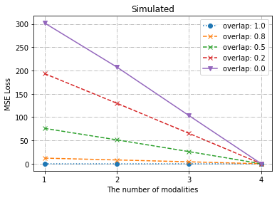
(b) Latent representation quality vs. The number of modalities on simulated data

Figure 2: Evaluation of the latent representation quality on different data sets

5.2 Synthetic Data

In this subsection, we investigate the effect of modality correlation on latent representation quality. Typically, there are three situations for the correlation across each modality [41]. (i) Each modality does not share information at all, that is, each modality only contains modal-specific information. (ii) The other is that, all modalities only maintain the share information without unique information on their own. (iii) The last is a moderate condition, i.e., each modal not only shares information, but also owns modal-specific information. The reason to utilize simulated data in this section is due to the fact that it is hard in practice to have natural datasets that possess the required degree of modality correlation.

Data Generation.

For the synthetic data, we have four modalities, denoted by $m_{1},m_{2},m_{3},m_{4}$, respectively, and the generation process is summarized as follows:

• Generate $m_{i}\sim\mathcal{N}(\mathbf{0},\mathbf{I})$, $i=1,2,3,4$, where $m_{i}$ is i.i.d. 100-dimensional random vector;

• Generate $m_{i}\leftarrow(1-w)\cdot m_{i}+w\cdot m_{1}$for $i=2,3,4$

• Generate the labels as follows. First, add the four modality vectors and calculate the sum of coordinates. Then, obatin the 1-dimensional label, i.e. $y=(m_{1}+m_{2}+m_{3}+m_{4}).sum(dim=1)$

We can see that information from $m_{1}$ is shared across different modalities, and $w$ controls how much is shared, which one can use to measure the degree of overlaps. We tune it in $\{0.0,0.2,0.5,0.8,1.0\}$. A high weight $w$ (close to $1$) indicates a high degree of overlaps, while $w=0$ means each modality is totally independent and is non-overlapping.

Training Setting.

We use the multi-layer perceptron neural network as our model. To be more specific, we first use a linear layer to encode the input to a $10$-dimension latent space and then we map the latent feature to the output space. The first layer’s input dimension depends on the number of modality. For example, if we use two modalities, the input dimension is $200$. We use SGD as our optimizer, and set a learning rate $0.01$, momentum $0.9$, batch size $10000$, training for $10000$ steps. The Mean Square Error (MSE) loss is considered for evaluation in this regression problem.

$\eta$ vs Modality Correlation

Our aim is to discover the influence of modality correlation on the latent representation quality $\eta$. To this end, Table 4 shows the $\eta$ with the varying number of modalities under different correlation conditions, which is measured by the MSE loss of the pretrain+finetuned modal. The trend that the loss decreases as the number of modalities increases is described in Figure 2(b), which also validates our analysis of Theorem 2. Moreover, Figure 2(b) shows that higher correlation among modalities achieves a lower loss for $\eta$, which means a better latent representation. This emphasizes the role of latent space to exploit the intrinsic correlations among different modalities.

Modalities	MSE Loss (Degree of Overlap )
	1	0.8	0.5	0.2	0.0
$m_{1}$	0	12.04$\pm$0.39	75.89$\pm$1.28	193.28$\pm$1.08	301.92$\pm$7.85
$m_{1},m_{2}$	0	8.16$\pm$0.17	51.25$\pm$1.06	129.81$\pm$4.36	207.45$\pm$4.68
$m_{1},m_{2},m_{3}$	0	4.18$\pm$0.05	26.06$\pm$0.69	65.17$\pm$1.52	103.23$\pm$0.61
$m_{1},m_{2},m_{3},m_{4}$	0	0	0	0	0

Table 4: Latent representation quality among different correlation situations on synthetic data

6 Discussion

It has been discovered that the use of multi-modal data in practice will degrade the performance of the model in some cases[45, 21, 40, 17]. These works identify the causes of performance drops of multi-modal as interactions between modalities in the training stage and try to improve the performance by proposing new optimization strategies. Therefore, to theoretically understand them, we need to analyze the training process from the optimization perspective. Our results, on the other hand, mainly focus on the generalization side, which is separated from optimization and assumes that we get the best performance possible in training. Moreover, our theory is general and does not require additional assumptions on the relationship across every single modality, which may be crucial for theoretically analyzing the observations in a multi-modal performance drop. Understanding why multi-modal fails in practice is a very interesting direction and worth further investigation in future research.

7 Conclusion

In this work, we formulate a multi-modal learning framework that has been extensively studied in the empirical literature towards rigorously understanding why multi-modality outperforms single since the former has access to a better latent space representation. The results answer the two questions: when and why multi-modal outperforms uni-modal jointly. To the best of our knowledge, this is the first theoretical treatment to explain the superiority of multi-modal from the generalization standpoint.

The key takeaway message is that the success of multi-modal learning relies essentially on the better quality of latent space representation, which points to an exciting direction that is worth further investigation: to find which encoder is the bottleneck and focus on improving it. More importantly, our work provides new insights for multi-modal theoretical research, and we hope this can encourage more related research.

Appendix A Proof of Main Results

A.1 Proof of Theorem 1

Proof.

Let $h^{\prime}_{\mathcal{M}}$ denote the minimizer of the population risk over $\mathcal{D}$ with the representation $\hat{g}_{\mathcal{M}}$, then we can decompose the difference between $r\left(\hat{h}_{\mathcal{M}}\circ\hat{g}_{\mathcal{M}}\right)-r\left(\hat{h}_{\mathcal{N}}\circ\hat{g}_{\mathcal{N}}\right)$ into two parts:

$$r\left(\hat{h}_{\mathcal{M}}\circ\hat{g}_{\mathcal{M}}\right)-r\left(\hat{h}_{\mathcal{N}}\circ\hat{g}_{\mathcal{N}}\right)$$ (15)

$$=\underbrace{r\left(\hat{h}_{\mathcal{M}}\circ\hat{g}_{\mathcal{M}}\right)-r\left(h^{\prime}_{\mathcal{M}}\circ\hat{g}_{\mathcal{M}}\right)}_{J_{1}}+\underbrace{r\left(h^{\prime}_{\mathcal{M}}\circ\hat{g}_{\mathcal{M}}\right)-r\left(\hat{h}_{\mathcal{N}}\circ\hat{g}_{\mathcal{N}}\right)}_{J_{2}}$$ (16)

$J_{1}$ can further be decomposed into:

$$J_{1}= \underbrace{r\left(\hat{h}_{\mathcal{M}}\circ\hat{g}_{\mathcal{M}}\right)-\hat{r}\left(\hat{h}_{\mathcal{M}}\circ\hat{g}_{\mathcal{M}}\right)}_{J_{11}}+\underbrace{\hat{r}\left(\hat{h}_{\mathcal{M}}\circ\hat{g}_{\mathcal{M}}\right)-\hat{r}\left(h^{\prime}_{\mathcal{M}}\circ\hat{g}_{\mathcal{M}}\right)}_{J_{12}}$$ (17)

$$+\underbrace{\hat{r}\left(h^{\prime}_{\mathcal{M}}\circ\hat{g}_{\mathcal{M}}\right)-r\left(h^{\prime}_{\mathcal{M}}\circ\hat{g}_{\mathcal{M}}\right)}_{J_{13}}$$ (18)

Clearly, $J_{12}\leq 0$ since $\hat{h}_{\mathcal{M}}$ is the minimizer of the empirical risk over $\mathcal{D}$ with the representation $\hat{g}_{\mathcal{M}}$. And $J_{11}+J_{13}\leq 2\sup_{h\in\mathcal{H},g_{\mathcal{M}}\in\mathcal{G}_{\mathcal{M}}}\left|r(h\circ g_{\mathcal{M}})-\hat{r}(h\circ g_{\mathcal{M}})\right|$.

$$\sup_{h\in\mathcal{H},g_{\mathcal{M}}\in\mathcal{G}_{\mathcal{M}}}\left|\hat{r}\left(h\circ g_{\mathcal{M}}\right)-r\left(h\circ g_{\mathcal{M}}\right)\right|$$

$$=\sup_{h\in\mathcal{H},g_{\mathcal{M}}\in\mathcal{G}_{\mathcal{M}}}\left|\frac{1}{m}\sum_{i=1}^{m}\ell\left(h\circ g_{\mathcal{M}}(\mathbf{x}_{i}),y_{i}\right)-\mathbb{E}_{(\mathbf{x}^{\prime},y^{\prime})\sim\mathcal{D}}\left[\ell\left(h\circ g_{\mathcal{M}}(\mathbf{x}^{\prime}),y^{\prime}\right)\right]\right|$$

Since $\ell$ is bounded by a constant $C$, we have $0\leq\ell\left(h\circ g_{\mathcal{M}}(\mathbf{x}),y\right)\leq C$ for any $(\mathbf{x},y)$. As one pair $(\mathbf{x}_{i},y_{i})$ changes, the above equation cannot change by at most $\frac{2C}{m}$. Applying McDiarmid’s[10] inequality, we obtain that with probability $1-\delta/2$:

$$\sup_{h\in\mathcal{H},g_{\mathcal{M}}\in\mathcal{G}_{\mathcal{M}}}\left|\hat{r}\left(h\circ g_{\mathcal{M}}\right)-r\left(h\circ g_{\mathcal{M}}\right)\right|$$ (20)

$$\leq \mathbb{E}_{(\mathbf{x}_{i},y_{i})\sim\mathcal{D}}\sup_{h\in\mathcal{H},g_{\mathcal{M}}\in\mathcal{G}_{\mathcal{M}}}\left|\frac{1}{m}\sum_{i=1}^{m}\ell\left(h\circ g_{\mathcal{M}}(\mathbf{x}_{i}),y_{i}\right)-\mathbb{E}_{(\mathbf{x}^{\prime},y^{\prime})\sim\mathcal{D}}\left[\ell\left(h\circ g_{\mathcal{M}}(\mathbf{x}^{\prime}),y^{\prime}\right)\right]\right|$$ (21)

$$+C\sqrt{\frac{2\ln(2/\delta)}{m}}$$ (22)

To proceed the proof, we introduce a popular result of Rademacher complexity in the following lemma[5]:

Lemma 1.

Let $U,\left\{U_{i}\right\}_{i=1}^{m}$ be i.i.d. random variables taking values in some space $\mathcal{U}$ and $\mathcal{F}\subseteq[a,b]^{\mathcal{U}}$ is a set of bounded functions. We have

$$\mathbb{E}\left[\sup_{f\in\mathcal{F}}\left(\mathbb{E}[f(U)]-\frac{1}{m}\sum_{i=1}^{m}f\left(U_{i}\right)\right)\right]\leq 2\mathfrak{R}_{m}(\mathcal{F})$$ (23)

Proof of lemma 1.

Denote $\left\{U^{\prime}_{i}\right\}_{i=1}^{m}$ be ghost examples of $\left\{U_{i}\right\}_{i=1}^{m}$, i.e. $U_{i}^{\prime}$ be independent of each other and have the same distribution as $U_{i}$. Then we have,

$$\mathbb{E}\left[\sup_{f\in\mathcal{F}}\left(\mathbb{E}[f(U)]-\frac{1}{m}\sum_{i=1}^{m}f\left(U_{i}\right)\right)\right]$$ (24)

$$= \mathbb{E}\left[\sup_{f\in\mathcal{F}}\left(\frac{1}{m}\sum_{i=1}^{m}\left(\mathbb{E}[f(U)]-f\left(U_{i}\right)\right)\right)\right]$$ (25)

$$\stackrel{{\scriptstyle(a)}}{{=}} \mathbb{E}\left[\sup_{f\in\mathcal{F}}\left(\frac{1}{m}\sum_{i=1}^{m}\mathbb{E}\left[f\left(U_{i}^{\prime}\right)-f\left(U_{i}\right)\mid\left\{U_{i}\right\}_{i=1}^{m}\right]\right)\right]$$ (26)

$$\leq \mathbb{E}\left[\mathbb{E}\left[\sup_{f\in\mathcal{F}}\left(\frac{1}{m}\sum_{i=1}^{m}\left(f\left(U_{i}^{\prime}\right)-f\left(U_{i}\right)\right)\right)\mid\left\{U_{i}\right\}_{i=1}^{m}\right]\right]$$ (27)

$$\stackrel{{\scriptstyle(b)}}{{=}} \mathbb{E}\left[\sup_{f\in\mathcal{F}}\left(\frac{1}{m}\sum_{i=1}^{m}\left(f\left(U_{i}^{\prime}\right)-f\left(U_{i}\right)\right)\right)\right]$$ (28)

$$= \mathbb{E}\left[\sup_{f\in\mathcal{F}}\left(\frac{1}{m}\sum_{i=1}^{m}\sigma_{i}\left(f\left(U_{i}^{\prime}\right)-f\left(U_{i}\right)\right)\right)\right]$$ (29)

$$\leq \mathbb{E}\left[\sup_{f\in\mathcal{F}}\frac{1}{m}\sum_{i=1}^{m}\sigma_{i}f\left(U_{i}^{\prime}\right)\right]+\mathbb{E}\left[\sup_{f\in\mathcal{F}}\frac{1}{m}\sum_{i=1}^{m}\sigma_{i}f\left(U_{i}\right)\right]$$ (30)

$$\stackrel{{\scriptstyle(c)}}{{=}} 2\mathfrak{R}_{m}(\mathcal{F}).$$ (31)

where $\sigma_{1},\ldots,\sigma_{m}$ is i.i.d. $\{\pm 1\}$ -valued random variables with $\mathbb{P}\left(\sigma_{i}=+1\right)=\mathbb{P}\left(\sigma_{i}=-1\right)=1/2$. $(a)$ $(b)$ are obtained by the tower property of conditional expectation; $(c)$ follows from the definition of Rademacher complexity of $\mathcal{F}$. ∎

Consider the function class:

$$\ell_{\mathcal{H}\circ\mathcal{G}_{\mathcal{M}}}:=\{(\mathbf{x},y)\mapsto\ell\left(h\circ g_{\mathcal{M}}(\mathbf{x}),y\right)\mid h\in\mathcal{H},g_{\mathcal{M}}\in\mathcal{G}_{\mathcal{M}}\}$$

let $\mathcal{F}=\ell_{\mathcal{H}\circ\mathcal{G}_{\mathcal{M}}}$ in lemma 1, then we have equation $(\ref{rad})$ can be upper bound by $2\mathfrak{R}_{m}(\ell_{\mathcal{H}\circ\mathcal{G}_{\mathcal{M}}})$. To directly work with the hypothesis function class, we need to decompose the Rademacher term which consists of the loss function classes. We center the function $\ell^{\prime}(h\circ g_{\mathcal{M}}(\mathbf{x}),y)=\ell(h\circ g_{\mathcal{M}}(\mathbf{x}),y)-\ell(\mathbf{0},y)$. The constant-shift property of Rademacher averages[5] indicates that

$$\mathfrak{R}_{m}(\ell_{\mathcal{H}\circ\mathcal{G}_{\mathcal{M}}})\leq\mathfrak{R}_{m}(\ell^{\prime}_{\mathcal{H}\circ\mathcal{G}_{\mathcal{M}}})+\frac{C}{\sqrt{m}}$$

Since $\ell^{\prime}$ is Lipschitz in its first coordinate with constant $L$ and $\ell^{\prime}(h\circ g_{\mathcal{M}}(\mathbf{0}),y)=0$, applying the contraction principle[5], we have:

$$\mathfrak{R}_{m}(\ell^{\prime}_{\mathcal{H}\circ\mathcal{G}_{\mathcal{M}}})\leq 2L\mathfrak{R}_{m}(\mathcal{H}\circ{G}_{\mathcal{M}})$$

Combining the above discussion, we obtain:

$$J_{1}\leq 8L\mathfrak{R}_{m}(\mathcal{H}\circ{G}_{\mathcal{M}})+\frac{4C}{\sqrt{m}}+2C\sqrt{\frac{2\ln(2/\delta)}{m}}$$

For $J_{2}$, by the definition of $h^{\prime}_{\mathcal{M}}$:

$$J_{2} =\inf_{h_{\mathcal{M}}\in\mathcal{H}}\left[r\left(h_{\mathcal{M}}\circ\hat{g}_{\mathcal{M}}\right)-r\left(\hat{h}_{\mathcal{N}}\circ\hat{g}_{\mathcal{N}}\right)\right]$$ (32)

$$\leq\sup_{h_{\mathcal{N}}\in\mathcal{H}}\inf_{h_{\mathcal{M}}\in\mathcal{H}}\left[r\left(h_{\mathcal{M}}\circ\hat{g}_{\mathcal{M}}\right)-r\left(h_{\mathcal{N}}\circ\hat{g}_{\mathcal{N}}\right)\right]$$ (33)

$$=\inf_{h_{\mathcal{M}}\in\mathcal{H}}\left[r\left(h_{\mathcal{M}}\circ\hat{g}_{\mathcal{M}}\right)-r(h^{*}\circ g^{*})\right]-\inf_{h_{\mathcal{N}}\in\mathcal{H}}\left[r\left(h_{\mathcal{N}}\circ\hat{g}_{\mathcal{N}}\right)-r(h^{*}\circ g^{*})\right]$$ (34)

$$=\eta(\hat{g}_{\mathcal{M}})-\eta(\hat{g}_{\mathcal{N}})$$ (35)

$$=\gamma_{\mathcal{S}}(\mathcal{M},\mathcal{N})$$ (36)

Finally,

$$r\left(\hat{h}_{\mathcal{M}}\circ\hat{g}_{\mathcal{M}}\right)-r\left(\hat{h}_{\mathcal{N}}\circ\hat{g}_{\mathcal{N}}\right)\leq\gamma_{\mathcal{S}}(\mathcal{M},\mathcal{N})+8L\mathfrak{R}_{m}(\mathcal{H}\circ\mathcal{G}_{\mathcal{M}})+\frac{4C}{\sqrt{m}}+2C\sqrt{\frac{2\ln(2/\delta)}{m}}$$

with probability $1-\frac{\delta}{2}$. ∎

A.2 Proof of Theorem 2

Proof.

Let $\tilde{h}_{\mathcal{M}}$ denote the minimizer of the population risk over $\mathcal{D}$ with the representation $\hat{g}_{\mathcal{M}}$, then we have:

$$\eta(\hat{g}_{\mathcal{M}})$$ (37)

$$=r(\tilde{h}_{\mathcal{M}}\circ\hat{g}_{\mathcal{M}})-r(h^{*}\circ g^{*})$$ (38)

$$\leq\underbrace{r(\hat{h}_{\mathcal{M}}\circ\hat{g}_{\mathcal{M}})-\hat{r}(\hat{h}_{\mathcal{M}}\circ\hat{g}_{\mathcal{M}})}_{J_{1}}+\underbrace{\hat{r}(\hat{h}_{\mathcal{M}}\circ\hat{g}_{\mathcal{M}})-\hat{r}(h^{*}\circ g^{*})}_{J_{2}}+\underbrace{\hat{r}(h^{*}\circ g^{*})-r(h^{*}\circ g^{*})}_{J_{3}}$$ (39)

$J_{2}$ is the centering empirical risk. Following the similar analysis in Theorem 1, we obtain:

$$J_{1}+J_{3} \leq\sup_{h\in\mathcal{H},g_{\mathcal{M}}\in\mathcal{G}_{\mathcal{M}}}\left|r(h\circ g_{\mathcal{M}})-\hat{r}(h\circ g_{\mathcal{M}})\right|+\sup_{h\in\mathcal{H},g\in\mathcal{G}}\left|r(h\circ g)-\hat{r}(h\circ g)\right|$$ (40)

$$\leq 4L\mathfrak{R}_{m}(\mathcal{H}\circ\mathcal{G}_{\mathcal{M}})+4L\mathfrak{R}_{m}(\mathcal{H}\circ\mathcal{G})+\frac{4C}{\sqrt{m}}+2C\sqrt{\frac{2\ln(2/\delta)}{m}}$$ (41)

with probability $1-\delta$. Combining the above discussion yields the result:

$$\eta(\hat{g}_{\mathcal{M}})\leq$$ (42)

$$4L\mathfrak{R}_{m}(\mathcal{H}\circ\mathcal{G}_{\mathcal{M}})+4L\mathfrak{R}_{m}(\mathcal{H}\circ\mathcal{G})+\frac{4C}{\sqrt{m}}+2C\sqrt{\frac{2\ln(2/\delta)}{m}}+\hat{L}(\hat{h}_{\mathcal{M}}\circ\hat{g}_{\mathcal{M}},\mathcal{S})$$ (43)

∎

A.3 Proof of Proposition 1

Proof.

With the $l_{2}$ loss, we have

$$\mathbb{E}_{\mathbf{x},y\sim h^{\star}\circ g^{\star}(\mathbf{x})}\{\ell(h\circ g(\mathbf{x}),y)-\ell(h^{\star}\circ g^{\star}(\mathbf{x}),y)\}=\mathbb{E}_{\mathbf{x}}\left[\left|\ \boldsymbol{\beta}^{\top}\mathbf{A}^{\top}\mathbf{x}-{\boldsymbol{\beta}^{\star}}^{\top}{\mathbf{A}^{\star}}^{\top}\mathbf{x}\right|^{2}\right]$$

Define the covariance matrix[43] for two linear projections $\mathbf{A}$, $\mathbf{A}^{\prime}$ as follows:

$$\Gamma(\mathbf{A},\mathbf{A}^{\prime})=\mathbb{E}_{\mathbf{x}}\left[\begin{array}[]{cc}\mathbf{A}^{\top}\mathbf{x}\left(\mathbf{A}^{\top}\mathbf{x}\right)^{\top}&\mathbf{A}^{\top}\mathbf{x}\left({\mathbf{A}^{\prime}}^{\top}\mathbf{x}\right)^{\top}\\ {\mathbf{A}^{\prime}}^{\top}\mathbf{x}\left(\mathbf{A}^{\top}\mathbf{x}\right)^{\top}&{\mathbf{A}^{\prime}}^{\top}\mathbf{x}\left({\mathbf{A}^{\prime}}^{\top}\mathbf{x}\right)^{\top}\end{array}\right]$$ (46)

$$=\left[\begin{array}[]{cc}\mathbf{A}^{\top}\Sigma\mathbf{A}&\mathbf{A}^{\top}\Sigma\mathbf{A}^{\prime}\\ {\mathbf{A}^{\prime}}^{\top}\Sigma\mathbf{A}&{\mathbf{A}^{\prime}}^{\top}\Sigma\mathbf{A}^{\prime}\end{array}\right]=\left[\begin{array}[]{cc}\Gamma_{11}(\mathbf{A},\mathbf{A}^{\star})&\Gamma_{12}(\mathbf{A},\mathbf{A}^{\star})\\ \Gamma_{21}(\mathbf{A},\mathbf{A}^{\star})&\Gamma_{22}(\mathbf{A},\mathbf{A}^{\star})\end{array}\right]$$ (51)

where $\Sigma$ denotes the covariance matrix of the distribution $\mathbb{P}_{\mathbf{x}}$. Then the latent representation quality of $\mathbf{A}$ becomes:

$$\eta(\mathbf{A}) =\inf_{\boldsymbol{\beta}:\|\boldsymbol{\beta}\|\leq C_{b}}\mathbb{E}_{\mathbf{x}}\left[\left|\ \boldsymbol{\beta}^{\top}\mathbf{A}^{\top}\mathbf{x}-{\boldsymbol{\beta}^{\star}}^{\top}{\mathbf{A}^{\star}}^{\top}\mathbf{x}\right|^{2}\right]$$ (52)

$$=\inf_{\boldsymbol{\beta}:\|\boldsymbol{\beta}\|\leq C_{b}}\left[\boldsymbol{\beta},-\boldsymbol{\beta}^{\star}\right]\Gamma(\mathbf{A},\mathbf{A}^{\star})\left[\boldsymbol{\beta},-\boldsymbol{\beta}^{\star}\right]^{\top}$$ (53)

For sufficiently large $C_{b}$, the constrained minimizer of $(\ref{mini})$ is equivalent to the unconstrained minimizer. Following the standard discussion of the quadratic convex optimization [6], if $\Gamma_{11}(\mathbf{A},\mathbf{A}^{\star})\succ 0$ and $\det\Gamma_{11}(\mathbf{A},\mathbf{A}^{\star})\not=0$, the solution of the above minimization problem is $\boldsymbol{\beta}=\Gamma_{11}(\mathbf{A},\mathbf{A}^{\star})^{-1}\Gamma_{12}(\mathbf{A},\mathbf{A}^{\star})\boldsymbol{\beta}^{\star}$, and

$$\eta(\mathbf{A})=\boldsymbol{\beta}^{\star}\Gamma_{sch}(\mathbf{A},\mathbf{A}^{\star}){\boldsymbol{\beta}^{\star}}^{\top}$$ (54)

where $\Gamma_{sch}(\mathbf{A},\mathbf{A}^{\star})$ is the Schur complement of $\Gamma(\mathbf{A},\mathbf{A}^{\star})$, defined as:

$$\Gamma_{sch}(\mathbf{A},\mathbf{A}^{\star})$$ (55)

$$=\Gamma_{22}(\mathbf{A},\mathbf{A}^{\star})-\Gamma_{21}(\mathbf{A},\mathbf{A}^{\star})\Gamma_{11}(\mathbf{A},\mathbf{A}^{\star})^{-1}\Gamma_{12}(\mathbf{A},\mathbf{A}^{\star})$$ (56)

Under the orthogonal assumption, $\hat{\mathbf{A}}_{\mathcal{M}}$ is nonsingular. Notice that $\hat{\mathbf{A}}_{\mathcal{N}}$ cannot be orthonormal in our settings. And $\sum$ is also invertible. Therefore, the Schur complement of $\Gamma(\hat{\mathbf{A}}_{\mathcal{M}},\mathbf{A}^{\star})$ exists,

$$\Gamma_{sch}(\hat{\mathbf{A}}_{\mathcal{M}},\mathbf{A}^{\star})={\mathbf{A}^{\star}}^{\top}\Sigma\mathbf{A}^{\star}-\left({\mathbf{A}^{\star}}^{\top}\Sigma\hat{\mathbf{A}}_{\mathcal{M}}\right)\left({\hat{\mathbf{A}}_{\mathcal{M}}}^{\top}\Sigma\hat{\mathbf{A}}_{\mathcal{M}}\right)^{-1}\left({\hat{\mathbf{A}}_{\mathcal{M}}}^{\top}\Sigma\mathbf{A}^{\star}\right)=\mathbf{0}$$ (57)

Hence, $\eta(\hat{\mathbf{A}}_{\mathcal{M}})=0$. Given the above discussion, we obtain:

$$\gamma_{\mathcal{S}}(\mathcal{M},\mathcal{N}) =\eta(\hat{\mathbf{A}}_{\mathcal{M}})-\eta(\hat{\mathbf{A}}_{\mathcal{N}})$$ (58)

$$=0-\inf_{\boldsymbol{\beta}:\|\boldsymbol{\beta}\|\leq C_{b}}\mathbb{E}_{\mathbf{x}}\left[\left|\ \boldsymbol{\beta}^{\top}\hat{\mathbf{A}}_{\mathcal{N}}^{\top}\mathbf{x}-{\boldsymbol{\beta}^{\star}}^{\top}{\mathbf{A}^{\star}}^{\top}\mathbf{x}\right|^{2}\right]\leq 0$$ (59)

∎

Appendix B The Composite Framework in Applications

As we stated in Section 3, our model well captures the essence of lots of existing multi-modal methods [3, 14, 16, 46, 45, 26]. Below, we explicitly discuss how these methods fit well into our general model, by providing the corresponding function class $\mathcal{G}$ under each method.

Audiovisual fusion for sound recognition [14]:

The audio and visual models map the respective inputs to segment-level representations, which are then used to obtain single-modal predictions, $\mathbf{h}_{a}$ and $\mathbf{h}_{v}$, respectively. The attention fusion function $n_{attn}$, ingests the single-modal predictions, $\mathbf{h}_{a}$ and $\mathbf{h}_{v}$, to produce weights for each modality, $\boldsymbol{\alpha}_{a}$ and $\boldsymbol{\alpha}_{v}$. The single-modal audio and visual predictions, $\mathbf{h}_{a}$ and $\mathbf{h}_{v}$, are mapped to $\tilde{\mathbf{h}}_{a}$ and $\tilde{\mathbf{h}}_{v}$ via functions $n_{a}$ and $n_{v}$ respectively, and fused using the attention weights, $\boldsymbol{\alpha}_{a}$ and $\boldsymbol{\alpha}_{v}$. In summary, $g$ has the form:

$$g=\tilde{\mathbf{h}}_{av}=\boldsymbol{\alpha}_{a}\odot\tilde{\mathbf{h}}_{a}+\boldsymbol{\alpha}_{v}\odot\tilde{\mathbf{h}}_{v}$$

Channel-Exchanging-Network [46]:

A feature map will be replaced by that of other modalities at the same position, if its scaling factor is lower than a threshold. $g$ in this problem can be formulated as a multi-dimensional mapping $g:=(f_{1},\cdots,f_{M})$, where subnetwork $f_{m}(x)$ adopts the multi-modal data $x$ as input and fuses multi-modal information by channel exchanging.

Other Fusion Methods [16, 45, 26, 3]:

Methods in these works can be formulated into the form we mentioned in the example in Section 3. Specifically, recall the example, $g$ has the form: $\varphi_{1}\oplus\varphi_{2}\oplus\cdots\oplus\varphi_{M}$, where $\oplus$ denotes a fusion operation, (e.g., averaging, concatenation, and self-attention), and $\varphi_{k}$ is a deep network which uses each modality data $x^{(k)}$ as input. Under these notations:

• For the early-fusion BERT method in [26], the temporal features are concatenated before the BERT layer and only a single BERT module is utilized. Here, the $\oplus$ is a concatenation function, and $g$ has the form $(\varphi_{1},\varphi_{2})$.

• [45, 16]discussed different fusion methods by choosing $\oplus$. (i) Max fusion: the $\oplus$ is the maximum function and $g:=max\left\{\varphi_{1},\cdots,\varphi_{M}\right\}$; (ii) Sum fusion: $g:=\sum\varphi_{m}$; (iii) averaging; (iv) self-attention and so on.

• The fusion section in the survey [3] provides many works which can be incorporated into our framework.

Appendix C Discussions on Training Setting

Existing works on multi-modal training demonstrates that naively fusing different modalities results insufficient representation learning of each modality [45, 11]. In our experiments, we train our multi-modal model using two methods: (1), naively end-to-end late-fusion training; (2), firstly train the uni-modal models and train a multi-modal classifier over the uni-modal encoders. As shown in Table 2 and Table 5, naively end-to-end training is unstable, affecting the representation learning of each modality, while fine-tuning a multi-modal classifier over trained uni-modal encoders is more stable and the results are more consistent with our theory. Noting that we use the late-fusion framework here, similar to  [45, 11].

Modalities	Test Acc (Ratio of Sample Size)
	$10^{-4}$	$10^{-3}$	$10^{-2}$	$10^{-1}$	1
T	23.66$\pm$1.28	29.08$\pm$3.34	45.63$\pm$0.29	48.30$\pm$1.31	49.93$\pm$0.57
TA	22.74$\pm$1.86	35.14$\pm$0.38	49.15$\pm$0.43	50.61$\pm$0.28	51.78$\pm$0.08
TV	23.64$\pm$0.07	36.64$\pm$1.79	46.91$\pm$0.68	48.96$\pm$0.47	53.24$\pm$0.35
TVA	25.40$\pm$1.06	40.87$\pm$2.47	50.67$\pm$0.63	52.54$\pm$0.60	54.55$\pm$0.29

Table 5: Latent representation quality vs. The number of the sample size on IEMOCAP. In this table, we fristly train the uni-modal models and train a multi-modal classifier over the uni-modal encoders to get multi-modal results.

References

- [1] Massih-Reza Amini, Nicolas Usunier, Cyril Goutte, et al. Learning from multiple partially observed views-an application to multilingual text categorization. In NIPS, volume 22, pages 28–36, 2009.
- [2] Peter Anderson, Qi Wu, Damien Teney, Jake Bruce, Mark Johnson, Niko Sünderhauf, Ian Reid, Stephen Gould, and Anton Van Den Hengel. Vision-and-language navigation: Interpreting visually-grounded navigation instructions in real environments. In Proceedings of the IEEE Conference on Computer Vision and Pattern Recognition, pages 3674–3683, 2018.
- [3] Tadas Baltrušaitis, Chaitanya Ahuja, and Louis-Philippe Morency. Multimodal machine learning: A survey and taxonomy. IEEE transactions on pattern analysis and machine intelligence, 41(2):423–443, 2018.
- [4] Peter Bartlett, Dylan J Foster, and Matus Telgarsky. Spectrally-normalized margin bounds for neural networks. arXiv preprint arXiv:1706.08498, 2017.
- [5] Peter L Bartlett and Shahar Mendelson. Rademacher and gaussian complexities: Risk bounds and structural results. Journal of Machine Learning Research, 3(Nov):463–482, 2002.
- [6] Stephen Boyd, Stephen P Boyd, and Lieven Vandenberghe. Convex optimization. Cambridge university press, 2004.
- [7] Carlos Busso, Murtaza Bulut, Chi-Chun Lee, Abe Kazemzadeh, Emily Mower, Samuel Kim, Jeannette N Chang, Sungbok Lee, and Shrikanth S Narayanan. Iemocap: Interactive emotional dyadic motion capture database. Language resources and evaluation, 42(4):335–359, 2008.
- [8] Giovanni Cavallanti, Nicolo Cesa-Bianchi, and Claudio Gentile. Linear algorithms for online multitask classification. The Journal of Machine Learning Research, 11:2901–2934, 2010.
- [9] Honglie Chen, Weidi Xie, Andrea Vedaldi, and Andrew Zisserman. Vggsound: A large-scale audio-visual dataset. In ICASSP 2020-2020 IEEE International Conference on Acoustics, Speech and Signal Processing (ICASSP), pages 721–725. IEEE, 2020.
- [10] Koby Crammer, Michael Kearns, and Jennifer Wortman. Learning from multiple sources. Journal of Machine Learning Research, 9(8), 2008.
- [11] Chenzhuang Du, Tingle Li, Yichen Liu, Zixin Wen, Tianyu Hua, Yue Wang, and Hang Zhao. Improving multi-modal learning with uni-modal teachers. arXiv preprint arXiv:2106.11059, 2021.
- [12] Simon S Du, Wei Hu, Sham M Kakade, Jason D Lee, and Qi Lei. Few-shot learning via learning the representation, provably. arXiv preprint arXiv:2002.09434, 2020.
- [13] Ariel Ephrat, Inbar Mosseri, Oran Lang, Tali Dekel, Kevin Wilson, Avinatan Hassidim, William T Freeman, and Michael Rubinstein. Looking to listen at the cocktail party: A speaker-independent audio-visual model for speech separation. arXiv preprint arXiv:1804.03619, 2018.
- [14] Haytham M Fayek and Anurag Kumar. Large scale audiovisual learning of sounds with weakly labeled data. arXiv preprint arXiv:2006.01595, 2020.
- [15] Marco Federici, Anjan Dutta, Patrick Forré, Nate Kushman, and Zeynep Akata. Learning robust representations via multi-view information bottleneck. arXiv preprint arXiv:2002.07017, 2020.
- [16] Christoph Feichtenhofer, Axel Pinz, and Andrew Zisserman. Convolutional two-stream network fusion for video action recognition. In Proceedings of the IEEE conference on computer vision and pattern recognition, pages 1933–1941, 2016.
- [17] Itai Gat, Idan Schwartz, Alexander Schwing, and Tamir Hazan. Removing bias in multi-modal classifiers: Regularization by maximizing functional entropies. arXiv preprint arXiv:2010.10802, 2020.
- [18] Jort F Gemmeke, Daniel PW Ellis, Dylan Freedman, Aren Jansen, Wade Lawrence, R Channing Moore, Manoj Plakal, and Marvin Ritter. Audio set: An ontology and human-labeled dataset for audio events. In 2017 IEEE International Conference on Acoustics, Speech and Signal Processing (ICASSP), pages 776–780. IEEE, 2017.
- [19] Yash Goyal, Tejas Khot, Douglas Summers-Stay, Dhruv Batra, and Devi Parikh. Making the v in vqa matter: Elevating the role of image understanding in visual question answering. In Proceedings of the IEEE Conference on Computer Vision and Pattern Recognition, pages 6904–6913, 2017.
- [20] Saurabh Gupta, Judy Hoffman, and Jitendra Malik. Cross modal distillation for supervision transfer. In Proceedings of the IEEE conference on computer vision and pattern recognition, pages 2827–2836, 2016.
- [21] Zongbo Han, Changqing Zhang, Huazhu Fu, and Joey Tianyi Zhou. Trusted multi-view classification. arXiv preprint arXiv:2102.02051, 2021.
- [22] Caner Hazirbas, Lingni Ma, Csaba Domokos, and Daniel Cremers. Fusenet: Incorporating depth into semantic segmentation via fusion-based cnn architecture. In Asian conference on computer vision, pages 213–228. Springer, 2016.
- [23] Kaiming He, Xiangyu Zhang, Shaoqing Ren, and Jian Sun. Deep residual learning for image recognition. In Proceedings of the IEEE conference on computer vision and pattern recognition, pages 770–778, 2016.
- [24] Xinxin Hu, Kailun Yang, Lei Fei, and Kaiwei Wang. Acnet: Attention based network to exploit complementary features for rgbd semantic segmentation. In 2019 IEEE International Conference on Image Processing (ICIP), pages 1440–1444. IEEE, 2019.
- [25] Jindong Jiang, Lunan Zheng, Fei Luo, and Zhijun Zhang. Rednet: Residual encoder-decoder network for indoor rgb-d semantic segmentation. arXiv preprint arXiv:1806.01054, 2018.
- [26] M Esat Kalfaoglu, Sinan Kalkan, and A Aydin Alatan. Late temporal modeling in 3d cnn architectures with bert for action recognition. In European Conference on Computer Vision, pages 731–747. Springer, 2020.
- [27] Diederik P Kingma and Jimmy Ba. Adam: A method for stochastic optimization. arXiv preprint arXiv:1412.6980, 2014.
- [28] Alex Krizhevsky, Ilya Sutskever, and Geoffrey E Hinton. Imagenet classification with deep convolutional neural networks. Advances in neural information processing systems, 25:1097–1105, 2012.
- [29] Mehryar Mohri, Afshin Rostamizadeh, and Ameet Talwalkar. Foundations of machine learning. MIT press, 2018.
- [30] Behnam Neyshabur, Zhiyuan Li, Srinadh Bhojanapalli, Yann LeCun, and Nathan Srebro. Towards understanding the role of over-parametrization in generalization of neural networks. arXiv preprint arXiv:1805.12076, 2018.
- [31] Behnam Neyshabur, Ryota Tomioka, and Nathan Srebro. Norm-based capacity control in neural networks. In Conference on Learning Theory, pages 1376–1401. PMLR, 2015.
- [32] Jiquan Ngiam, Aditya Khosla, Mingyu Kim, Juhan Nam, Honglak Lee, and Andrew Y Ng. Multimodal deep learning. In ICML, 2011.
- [33] Seong-Jin Park, Ki-Sang Hong, and Seungyong Lee. Rdfnet: Rgb-d multi-level residual feature fusion for indoor semantic segmentation. In Proceedings of the IEEE international conference on computer vision, pages 4980–4989, 2017.
- [34] Massimiliano Pontil and Andreas Maurer. Excess risk bounds for multitask learning with trace norm regularization. In Conference on Learning Theory, pages 55–76. PMLR, 2013.
- [35] Soujanya Poria, Erik Cambria, Devamanyu Hazarika, Navonil Majumder, Amir Zadeh, and Louis-Philippe Morency. Context-dependent sentiment analysis in user-generated videos. In Proceedings of the 55th annual meeting of the association for computational linguistics (volume 1: Long papers), pages 873–883, 2017.
- [36] George AF Seber and Alan J Lee. Linear regression analysis, volume 329. John Wiley & Sons, 2012.
- [37] Daniel Seichter, Mona Köhler, Benjamin Lewandowski, Tim Wengefeld, and Horst-Michael Gross. Efficient rgb-d semantic segmentation for indoor scene analysis. arXiv preprint arXiv:2011.06961, 2020.
- [38] Linda Smith and Michael Gasser. The development of embodied cognition: Six lessons from babies. Artificial life, 11(1-2):13–29, 2005.
- [39] Karthik Sridharan and Sham M Kakade. An information theoretic framework for multi-view learning. 2008.
- [40] Mahesh Subedar, Ranganath Krishnan, Paulo Lopez Meyer, Omesh Tickoo, and Jonathan Huang. Uncertainty-aware audiovisual activity recognition using deep bayesian variational inference. In Proceedings of the IEEE/CVF International Conference on Computer Vision, pages 6301–6310, 2019.
- [41] Xinwei Sun, Yilun Xu, Peng Cao, Yuqing Kong, Lingjing Hu, Shanghang Zhang, and Yizhou Wang. Tcgm: An information-theoretic framework for semi-supervised multi-modality learning. In European Conference on Computer Vision, pages 171–188. Springer, 2020.
- [42] Nilesh Tripuraneni, Chi Jin, and Michael I Jordan. Provable meta-learning of linear representations. arXiv preprint arXiv:2002.11684, 2020.
- [43] Nilesh Tripuraneni, Michael Jordan, and Chi Jin. On the theory of transfer learning: The importance of task diversity. Advances in Neural Information Processing Systems, 33, 2020.
- [44] Yao-Hung Hubert Tsai, Yue Wu, Ruslan Salakhutdinov, and Louis-Philippe Morency. Self-supervised learning from a multi-view perspective. arXiv preprint arXiv:2006.05576, 2020.
- [45] Weiyao Wang, Du Tran, and Matt Feiszli. What makes training multi-modal classification networks hard? In 2020 IEEE/CVF Conference on Computer Vision and Pattern Recognition (CVPR), pages 12692–12702. IEEE, 2020.
- [46] Yikai Wang, Wenbing Huang, Fuchun Sun, Tingyang Xu, Yu Rong, and Junzhou Huang. Deep multimodal fusion by channel exchanging. Advances in Neural Information Processing Systems, 33, 2020.
- [47] Chang Xu, Dacheng Tao, and Chao Xu. A survey on multi-view learning. arXiv preprint arXiv:1304.5634, 2013.
- [48] Dan Xu, Wanli Ouyang, Elisa Ricci, Xiaogang Wang, and Nicu Sebe. Learning cross-modal deep representations for robust pedestrian detection. In Proceedings of the IEEE conference on computer vision and pattern recognition, pages 5363–5371, 2017.
- [49] Yang Yang, Han-Jia Ye, De-Chuan Zhan, and Yuan Jiang. Auxiliary information regularized machine for multiple modality feature learning. In Twenty-Fourth International Joint Conference on Artificial Intelligence, 2015.
- [50] Changqing Zhang, Huazhu Fu, Joey Tianyi Zhou, Qinghua Hu, et al. Cpm-nets: Cross partial multi-view networks. 2019.
- [51] Hang Zhao, Chuang Gan, Andrew Rouditchenko, Carl Vondrick, Josh McDermott, and Antonio Torralba. The sound of pixels. In Proceedings of the European conference on computer vision (ECCV), pages 570–586, 2018.
- [52] Tao Zhou, Kim-Han Thung, Mingxia Liu, Feng Shi, Changqing Zhang, and Dinggang Shen. Multi-modal latent space inducing ensemble svm classifier for early dementia diagnosis with neuroimaging data. Medical image analysis, 60:101630, 2020.