Back2Future: Leveraging Backfill Dynamics for Improving Real-time Predictions in Future

Abstract

For real-time forecasting in domains like public health and macroeconomics, data collection is a non-trivial and demanding task. Often after being initially released, it undergoes several revisions later (maybe due to human or technical constraints) - as a result, it may take weeks until the data reaches a stable value. This so-called ‘backfill’ phenomenon and its effect on model performance have been barely addressed in the prior literature. In this paper, we introduce the multi-variate backfill problem using COVID-19 as the motivating example. We construct a detailed dataset composed of relevant signals over the past year of the pandemic. We then systematically characterize several patterns in backfill dynamics and leverage our observations for formulating a novel problem and neural framework, Back2Future, that aims to refines a given model’s predictions in real-time. Our extensive experiments demonstrate that our method refines the performance of diverse set of top models for COVID-19 forecasting and GDP growth forecasting. Specifically, we show that Back2Future refined top COVID-19 models by 6.65% to 11.24% and yield 18% improvement over non-trivial baselines. In addition, we show that our model improves model evaluation too; hence policy-makers can better understand the true accuracy of forecasting models in real-time.

1 Introduction

The current COVID-19 pandemic has challenged our response capabilities to large disruptive events, affecting the health and economy of millions of people. A major tool in our response has been forecasting epidemic trajectories, which has provided lead time to policymakers to optimize and plan interventions (Holmdahl & Buckee, 2020). Broadly two classes of approaches have been devised: traditional mechanistic epidemiological models (Shaman & Karspeck, 2012; Zhang et al., 2017), and the fairly newer statistical approaches (Brooks et al., 2018; Adhikari et al., 2019; Osthus et al., 2019b) including deep learning models (Adhikari et al., 2019; Deng et al., 2020; Panagopoulos et al., 2021; Rodríguez et al., 2021a), which have become among the top-performing ones for multiple forecasting tasks (Reich et al., 2019). These also leverage newer digital indicators like search queries (Ginsberg et al., 2009; Yang et al., 2015) and social media (Culotta, 2010; Lampos et al., 2010). As noted in multiple previous works (Metcalf & Lessler, 2017; Biggerstaff et al., 2018), epidemic forecasting is a challenging enterprise because it is affected by weather, mobility, strains, and others.

However, real-time forecasting also brings new challenges. As noted in multiple CDC real-time forecasting initiatives for diseases like flu (Osthus et al., 2019a) and COVID-19 (Cramer et al., 2021), as well as in macroeconomics (Clements & Galvão, 2019; Aguiar, 2015) the initially released public health data is revised many times after and is known as the ’backfill’ phenomenon.The various factors that affect backfill are multiple and complex, ranging from surveillance resources to human factors like coordination between health institutes and government organizations within and across regions (Chakraborty et al., 2018; Reich et al., 2019; Altieri et al., 2021; Stierholz, 2017).

While previous works have addressed anomalies (Liu et al., 2017), missing data (Yin et al., 2020), and data delays (Žliobaite, 2010) in general time-series problems, the backfill problem has not been addressed. In contrast, the topic of revisions has not received as much attention, with few exceptions. For example in epidemic forecasting, a few papers have either (a) mentioned about the ‘backfill problem’ and its effects on performance (Chakraborty et al., 2018; Rodríguez et al., 2021b; Altieri et al., 2021; Rangarajan et al., 2019) and evaluation (Reich et al., 2019); or (b) proposed to address the problem via simple models like linear regression (Chakraborty et al., 2014) or ’backcasting’ (Brooks et al., 2018) the observed targets c) used data assimilation and sensor fusion from a readily available stable set of features to refine unrevised features (Farrow, 2016; Osthus et al., 2019a). However, they focus only on revisions in the target and typically study in the context of influenza forecasting, which is substantially less noisy and more regular than the novel COVID-19 pandemic or assume access to stable values for some features which is not the case for COVID-19. In economics, Clements & Galvão (2019) surveys several domain-specific (Carriero et al., 2015) or essentially linear techniques for data revision/correction behavior of several macroeconomic indicators (Croushore, 2011).

Motivated from above, we study the more challenging problem of multi-variate backfill for both features and targets. We go further beyond prior work and also show how to leverage our insights for a more general neural framework to improve both predictions (i.e. refinement of the model’s predictions) and performance evaluation (i.e. rectification from the evaluator’s perspective). Our specific contributions are the following:

$\bullet$ Multi-variate backfill problem: We introduce the multi-variate backfill problem using real-time epidemiological forecasting as the primary motivating example. In this challenging setting, which generalizes (the limited) prior work, the forecast targets, as well as exogenous features, are subject to retrospective revision. Using a carefully collected diverse dataset for COVID-19 forecasting for the past year, we discover several patterns in backfill dynamics, show that there is a significant difference in real-time and revised feature measurements, and highlight the negative effects of using unrevised features for incidence forecasting in different models both for model performance and evaluation. Building on our empirical observations, we formulate the problem Bfrp, which aims to ‘correct’ given model predictions to achieve better performance on eventual fully revised data.

$\bullet$ Spatial and Feature level backfill modeling to refine model predictions: Motivated by the patterns in revision and observations from our empirical study, we propose a deep-learning model Back2Future (B2F) to model backfill revision patterns and derive latent encodings for features. B2F combines Graph Convolutional Networks that capture sparse, cross-feature, and cross-regional backfill dynamics similarity and deep sequential models that capture temporal dynamics of each features’ backfill dynamics across time. The latent representation of all features is used along with the history of the model’s predictions to improve diverse classes of models trained on real-time targets, to predict targets closer to revised ground truth values. Our technique can be used as a ‘wrapper’ to improve model performance of any forecasting model (mechanistic/statistical).

$\bullet$ Refined top models’ predictions and improved model evaluation: We perform an extensive empirical evaluation to show that incorporating backfill dynamics through B2F consistently improves the performance of diverse classes of top-performing COVID-19 forecasting models (from the CDC COVID-19 Forecast Hub, including the top-performing official ensemble) significantly. We also utilize B2F to help forecast evaluators and policy-makers better evaluate the ‘eventual’ true accuracy of participating models (against revised ground truth, which may not be available until weeks later). This allows the model evaluators to quickly estimate models that perform better w.r.t revised stable targets instead of potentially misleading current targets. Our methodology can be adapted for other time-series forecasting problems in general. We also show the generalizability of our framework and model B2F to other domains by significantly improving predictions of non-trivial baselines for US National GDP forecasting (Marcellino, 2008; Tkacz & Hu, 1999).

2 Nature of backfill dynamics

In this section, we study important properties of the revision dynamics of our signals. We introduce some concepts and definitions to aid in the understanding of our empirical observations and method.

Real-time forecasting. We are given a set of signals $\mathcal{F}=\mathrm{Reg}\times\mathrm{Feat}$, where $\mathrm{Reg}$ is the set of all regions (where we want to forecast) and set $\mathrm{Feat}$ contains our features and forecasting target(s) for each region. At prediction week $t$, $x^{(t)}_{i,1:t}$ is a time series from 1 to $t$ for feature $i$, and the set of all signals results in the multi-variate time series $\mathcal{X}^{(t)}_{1:t}$. Similarly, $\mathcal{Y}^{(t)}_{1:t}$ is the forecasting target(s) time series. Further, let’s call all data available at time $t$, $\mathcal{D}^{(t)}_{1:t}=\{\mathcal{X}^{(t)}_{1:t},\mathcal{Y}^{(t)}_{1:t}\}$ as real-time sequence. For clarity we refer to ‘signal’ $i\in\mathcal{F}$ as a sequence of either a feature or a target, and denote it as $d^{(t)}_{i,1:t}$. Thus, at prediction week $t$, the real-time forecasting problem is: Given $\mathcal{D}^{(t)}_{1:t}$, predict next $k$ values of forecasting target(s), i.e. $\hat{y}_{t+1:t+k}$. Typically for CDC settings and this paper, our time unit is week, $k=4$ (up to 4 weeks ahead) and our target is COVID-19 mortality incidence (Deaths).

Revisions. Data revisions (‘backfill’) are common. At prediction week $t+1$, the real-time sequence $\mathcal{D}^{(t+1)}_{1:t+1}$ is available. In addition to the length of the sequences increasing by one (new data point), values of $\mathcal{D}^{(t+1)}_{1:t+1}$ already in $\mathcal{D}^{(t)}_{1:t}$ may be revised i.e., $\mathcal{D}^{(t)}_{1:t}\neq\mathcal{D}^{(t+1)}_{1:t}$. Note that previous work has studied backfill limited to $\mathcal{Y}^{(t)}$, while we address it in both $\mathcal{X}^{(t)}$ and $\mathcal{Y}^{(t)}$. Also, note that the data in the backfill is the same used for real-time forecasting, but just seen from a different perspective.

Backfill sequences: Another useful way we propose to look at backfill is by focusing on revisions of a single value. Let’s focus on value of signal $i$ at an observation week $t^{\prime}$. For this observation week, the value of the signal can be revised at any $t>t^{\prime}$, which induces a sequence of revisions. We refer to revision week $r\geq 0$ as the relative amount of time that has passed since the observation week $t^{\prime}$.

Defn. 1.

(Backfill Sequence BSeq) For signal $i$ and observation week $t^{\prime}$, its backfill sequence is $\textsc{BSeq}(i,t^{\prime})=\langle d_{i,t^{\prime}}^{(t^{\prime})},d_{i,t^{\prime}}^{(t^{\prime}+1)},\ldots,d_{i,t^{\prime}}^{(\infty)}\rangle$, where $d_{i,t^{\prime}}^{(t^{\prime})}$ is the initial value of the signal and $d_{i,t^{\prime}}^{(\infty)}$ is the final/stable value of the signal.

Defn. 2.

(Backfill Error BErr) For revision week $r$ of a backfill sequence, the backfill error is $\textsc{BErr}(r,i,t^{\prime})=|d^{(t^{\prime}+r)}_{i,t^{\prime}}-d^{(\infty)}_{i,t^{\prime}}|~{}/~{}|d^{(\infty)}_{i,t^{\prime}}|.$

Defn. 3.

(Stability time STime) of a backfill sequence BSeq is the revision week $r^{*}$ that is the minimum $r$ for which the backfill error BErr $<\epsilon$ for all $r>r^{*}$, i.e., the time when BSeq stabilizes.

Note: We ensured that BSeq length is at least 7, and found that in our dataset most signals stabilize before $r=20$. For $d^{(\infty)}_{i,t^{\prime}}$, we use $d^{(t_{f})}_{i,t^{\prime}}$, at the final week $t_{f}$ in our revisions dataset. In case we do not find $\textsc{BErr}<\epsilon$ in any BSeq, we set STime to the length of that BSeq. We use $\epsilon=0.05$. Example: For BSeq $\{223,236,236,404,\dots,404\}$, BErr for third week is $\frac{|236-404|}{404}=0.41$ and STime is 4.

2.1 Dataset description

Table 1: List of features in our CoVDS

Type	Features
Patient Line-List	ERVisits, HospRate, +veInc, HospInc, Recovered, onVentilator, inICU
Testing	TestResultsInc, -veInc, Facilities
Mobility	RetailRec, Grocery, Parks, Transit, WorkSpace, Resident, AppleMob
Exposure	DexA
Social Survey	FbCLI, FbWiLi

We collected important publicly available signals from a variety of trusted sources that are relevant to COVID-19 forecasting to form the COVID-19 Surveillance Dataset (CoVDS). See Table 1 for the list of 20 features ($|\mathrm{Feat}|=21$, including Deaths). Our revisions dataset contains signals that we collected every week since April 2020 and ends on July 2021. Our analysis covers $30$ observation weeks from June 2020 to December 2020 (to ensure all our backfill sequences are of length at least 7) for all $|\mathrm{Reg}|=50$ US states. The rest of the unseen data from Jan 2021 to July 2021 is used strictly for evaluation.

Patient line-list: traditional surveillance signals used in epidemiological models (Chakraborty et al., 2014; Brooks et al., 2018) derived from line-list records e.g. hospitalizations from CDC (CDC, 2020), positive cases, ICU admissions from COVID Tracking (COVID-Tracking, 2020). Testing: measure changes in testing from CDC and COVID-Tracking e.g. tested population, negative tests, used by Rodríguez et al. (2021b). Mobility: track people movement to several point of interests (POIs), from Google (2020) and Apple (2020), and serve as digital proxy for social distancing (Arik et al., 2020). Exposure: digital signal measuring closeness between people at POIs, collected from mobile phones (Chevalier et al., 2021) Social Survey: previously used by (Wang et al., 2020; Rodríguez et al., 2021b) CMU/Facebook Symptom Survey Data, which contains self-reported responses about COVID-19 symptoms.

2.2 Observations

We first study different facets of the significance of backfill in CoVDS. Using our definitions, we generate a backfill sequence for every combination of signal, observation week, and region (not all signals are available for all regions). In total, we generate more than $30,000$ backfill sequences.

Backfill error BErr is significant. We computed BErr for the initial values, i.e., $\textsc{BErr}(r=0,i,t^{\prime})$, for all signals $i$ and observation weeks $t^{\prime}$.

Obs. 1.

(BErr across signals and regions) Compute the average BErr for each signal; the median of all these averages is $32\%$, i.e. at least half of all signals are corrected by $32\%$ of their initial value. Similarly in at least half of the regions the signal corrections are 280% of their initial value.

We also found large variation of BErr. For features (Figure 1a), compare avg. $\textsc{BErr}=1743\%$ of five most corrected features with $1.6\%$ of the five least corrected features. Also, in contrast to related work that focuses on traditional surveillance data Yang et al. (2015), perhaps unexpectedly, we found that digital indicators also have a significant BErr (average of $108\%$). For regions (see Figure 1b), compare $1594\%$ of the five most corrected regions with $38\%$ of the five least corrected regions.

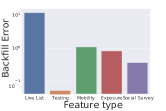
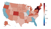
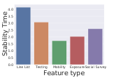
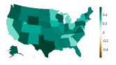
(a) BErr per feat. type	(b) BErr per region	(c) STime per feat. type	(d) STime per region

Figure 1: BErr and STime across feature type and regions, heat maps are $\log$ scaled.

Stability time STime is significant. A similar analysis for STime found significant variation across signals (from 1 weeks for to 21 weeks for COVID-19, see Figure 1c for STime across feature types) and regions (from 1.55 weeks for GA to 3.83 weeks for TX, see Figure 1d). This also impacts our target, thus, actual accuracy is not readily available which undermines real-time evaluation and decision making.

Obs. 2.

(STime of features and target) Compute the average STime for each signal; the average of all these averages for features is around 4 weeks and for our target Deaths is around 3 weeks, i.e. on average, it takes over 3 weeks to reach the stable values of features.

Backfill sequence BSeq patterns. There is significant similarity among BSeqs. We cluster BSeqs via K-means using Dynamic Time Warping (DTW) as pair-wise distance (as DTW can handle sequences of varying magnitude and length). We found five canonical categories of behaviors (see Figure 2), each of size roughly 11.58% of all BSeqs.

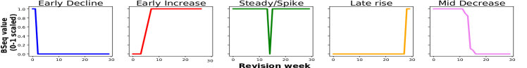
Figure 2: Centroid BSeq of each cluster, scaled between $[0,1]$, showing canonical backfill behaviors

Also, each cluster is not defined only by signal nor region. Hence there is a non-trivial similarity across both signals and regions.

Obs. 3.

(BSeq similarity and variety) Five canonical behaviors were observed in our backfill sequences (Figure 2). No cluster has over 21% of BSeqs from the same region, and no cluster has over 14% of BSeqs from the same signal.

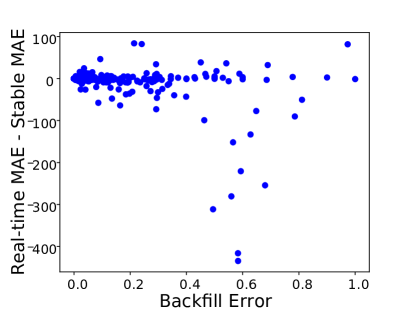
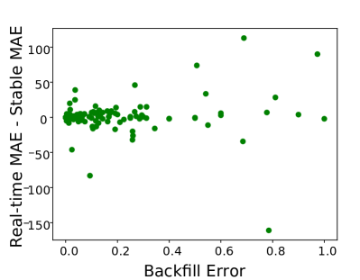
(a) GT-DC	(b) YYG

Figure 3: BErr vs model RevDiffMAE.

Model performance vs BErr. To study the relationship between model performance (via Mean Absolute Error MAE of a prediction) and BErr, we use RevDiffMAE: the difference between MAE computed against real-time target value and one against the stable target value. We analyze the top-performing real-time forecasting models as per the comprehensive evaluation of all models in COVID-19 Forecast Hub (Cramer et al., 2021). YYG and UMass-MB are mechanistic while CMU-TS and GT-DC are statistical models. The top performing Ensemble is composed of all contributing models to the hub. We expect a well-trained real-time model will have higher RevDiffMAE with larger BErr in its target (Reich et al., 2019). However, we found that higher BErr does not necessarily mean worse performance. See Figure 3—YYG has even better performance with more revisions. This may be due to the more complex backfill activity/dependencies in COVID in comparison to the more regular seasonal flu.

Obs. 4.

(Model performance and backfill) Relation between BErr and RevDiffMAE can be non-monotonous and positively or negatively correlated depending on model and signal.

Real-time target values to measure model performance: Since targets undergo revisions (5% BErr on average), we study how this BErr affects the real-time evaluation of models. From Figure 4, we see that the scores are not similar with real-time scores over-estimating model accuracy. The average difference in scores is positive which implies that evaluators would overestimate models’ forecasting ability.

Obs. 5.

MAE evaluated at real-time overestimates model performance by 9.6 on average, with the maximum for TX at 22.63.

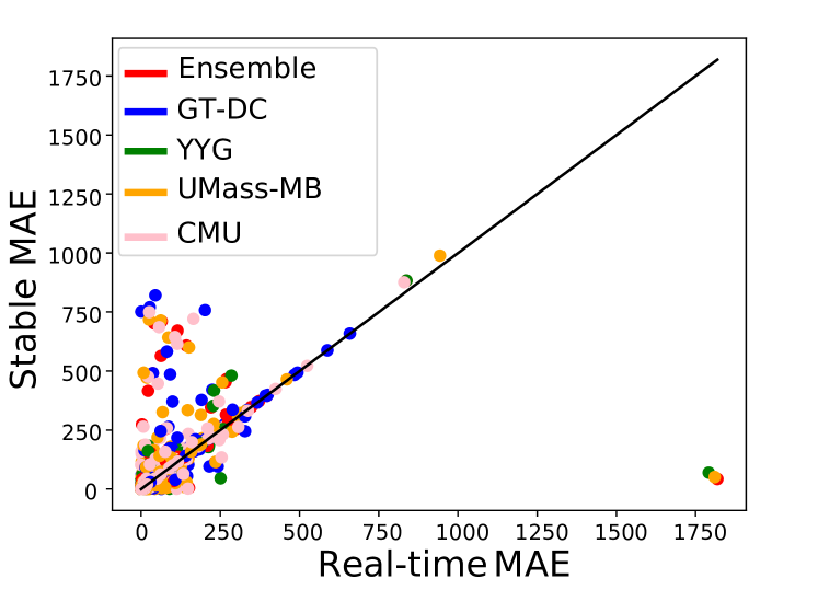
Figure 4: Real-time vs stable MAE.

3 Refining the future via B2F

Our observations naturally motivate improving training and evaluation aspects of real-time forecasting by leveraging revision information. Thus, we propose the following two problems. Let predictions of model $M$ for week $t+k$ be $y(M,k)_{t}$. Since models are trained on real-time targets, $y(M,k)_{t}$ is the model’s estimate of target $y_{t+k}^{(t+k)}$.

$k$-week ahead Backfill Refinement Problem, $\textsc{Bfrp}_{k}(M)$: At prediction week $t$, we are given a revision dataset $\{\mathcal{D}_{1:t^{\prime}}^{(t^{\prime})}\}_{t^{\prime}\leq t}$, which includes our target $\mathcal{Y}^{(t)}_{1:t}$. For a model $M$ trained on real-time targets, given history of model’s predictions till last week $\langle y(M,k)_{1},\dots y(M,k)_{t-1}\rangle$ and prediction for current week $y(M,k)_{t}$, our goal is to refine $y(M,k)_{t}$ to better estimate the stable target $y_{t+k}^{(t_{f})}$, i.e. the ’future’ of our target value at $t+k$.

Leaderboad Refinement problem, Lbrp: At each week $t$, evaluators are given a current estimate of our target $y_{t}^{(t)}$ and forecasts of models submitted on week $t-k$. Our goal is to refine $y_{t}^{(t)}$ to $\hat{y}_{t}$, a better estimate of $y_{t}^{(t_{f})}$, so that using $\hat{y}_{t}$ as a surrogate for $y_{t}^{(t_{f})}$ to evaluate predictions of models provides a better indicator of their actual performance (i.e., we obtain a refined leaderboard of models). Relating it to Bfrp, assume a hypothetical model $M_{eval}$ whose predictions are real-time ground truth, i.e. $y(M_{eval},0)_{t}=y_{t}^{(t)},\forall t$. Then, refining $M_{eval}$ is equivalent to refining $y_{t}^{(t)}$ to better estimate $y_{t}^{(t_{f})}$ which leads to solving Lbrp. Thus, Lbrp is a special case of $\textsc{Bfrp}_{0}(M_{eval})$.

Overview: We leverage observations from Section 2 to derive Back2Future (B2F), a deep-learning model that uses revision information from BSeq to refine predictions. Obs. 1 and 2 show that real-time values of signals are poor estimates of stable values. Therefore, we leverage patterns in BSeq of past signals and exploit cross-signal similarities (Obs. 3) to extract information from BSeqs. We also consider that the relation of models’ forecasts to BErr of targets is complex (Obs. 4 and 5) to refine their predictions. B2F combines these ideas through its four modules: $\bullet$ GraphGen: Generates a signal graph (where each node maps to a signal in $\mathrm{Reg}\times\mathrm{Feat}$) whose edges are based on BSeq similarities. $\bullet$ BseqEnc: Leverages the signal graph as well as temporal dynamics of BSeqs to learn a latent representation of BSeqs using a Recurrent Graph Neural Network. $\bullet$ ModelPredEnc: Encodes the history of the model’s predictions, the real-time value of the target, and past revisions of the target through a recurrent neural network. $\bullet$ Refiner: Combines encodings from BseqEnc and ModelPredEnc to predict the correction to model’s real-time prediction.

In contrast to previous works that studies target BErr (Reich et al., 2019), we simultaneously model all BSeq available till current week $t$ using spatial and signal similarities in the temporal dynamics of BSeq. Recent works that attempt to model spatial relations for COVID19 forecasting need explicitly structural data (like cross-region mobility) (Panagopoulos et al., 2020) to generate a graph or use attention over temporal patterns of regions’ death trends. B2F, in contrast, directly models the structural information of signal graph (containing features from each region) using BSeq similarities. Thus, we first generate useful latent representations for each signal based on BSeq revision information of that feature as well as features that have shown similar revision patterns in the past. Due to the large number of signals that cover all regions, we cannot model the relations between every pair using fully connected modules or attention similar to (Jin et al., 2020). Therefore, we first construct a sparse graph between signals based on past BSeq similarities. Then we inject this similarity information using Graph Convolutional Networks (GCNs) and combine it with deep sequential models to model temporal dynamics of BSeq of each signal while combining information from BSeq s of signals in the neighborhood of the graph. Further, we use these latent representations and leverage the history of a model $M$’s predictions to refine its prediction. Thus, B2F solves $\textsc{Bfrp}_{k}(M)$ assuming $M$ is a black box, accessing only its past forecasts. Our training process, that involves pre-training on model-agnostic auxiliary task, greatly improves training time for refining any given model $M$. The full pipeline of B2F is also shown in Figure 5. Next, we describe each of the components of B2F in detail. For the rest of this section, we will assume that we are forecasting $k$ weeks ahead given data till current week $t$.

Figure 5: B2F pipeline with all components

GraphGen generates an undirected signal graph $G_{t}=(V,E_{t})$ whose edges represent similarity in BSeqs between signals, where vertices $V=\mathcal{F}=\mathrm{Reg}\times\mathrm{Feat}$. We measure similarity using DTW distance due to reasons described in Section 2. GraphGen leverages the similarities across BSeq patterns irrespective of the exact nature of canonical behaviors which may vary across domains. We compute the sum of DTW distances of BSeqs for each pair of nodes summed over $t^{\prime}\in\{1,2,\dots,t-5\}$. We threshold $t^{\prime}$ till $t-5$ to make the BSeqs to be of reasonable length (at least 5) to capture temporal similarity without discounting too many BSeqs. Top $\tau$ node pairs with lowest total DTW distance are assigned an edge.

BseqEnc. While we can model backfill sequences for each signal independently using a recurrent neural network, this doesn’t capture the behavioral similarity of BSeq across signals. Using a fully-connected recurrent neural network that considers all possible interactions between signals also may not learn from the similarity information due to the sheer number of signals ($50\times 21=1050$) while greatly increasing the parameters of the model. Thus, we utilize the structural prior of graph $G_{t}$ generated by GraphGen and train an autoregressive model BseqEnc which consists of graph recurrent neural network to encode a latent representation for each of backfill sequence in $B_{t}=\{\textsc{BSeq}(i,t):i\in\mathcal{F}\}$. At week $t$, BseqEnc is first pre-trained and then it is fine-tuned for a specific model $M$ (more details later in this section).

Our encoding process is in Figure 5. Let $\textsc{BSeq}_{t^{\prime}+r}(i,t^{\prime})$ be first $r+1$ values of $\textsc{BSeq}(i,t^{\prime})$ (till week $t^{\prime}+r$). For a past week $t^{\prime}$ and revision week $r$, we denote $h_{i,t^{\prime}}^{(t^{\prime}_{r})}\in\mathrm{R}^{m}$ to be the latent encoding of $\textsc{BSeq}_{t^{\prime}_{r}}(i,t^{\prime})$ where $t^{\prime}_{r}=t^{\prime}+r$ and $t^{\prime}\leq t^{\prime}_{r}\leq t$. We initialize $h_{i,t^{\prime}}^{(0)}$ for any observation week $t^{\prime}$ to be a learnable parameter $h_{i}^{(0)}\in\mathrm{R}^{m}$ specific to signal $i$. For each week $t^{\prime}_{r}$ we combine latent encoding $h_{i,t^{\prime}}^{(t^{\prime}_{r}-1)}$ and signal value $d_{i,t^{\prime}}^{(t^{\prime}_{r})}$ using a GRU (Gated Recurrent Unit) (Cho et al., 2014) cell to get the intermediate embedding $v_{i,t}^{(t^{\prime})}$. Then, we leverage the signal graph $G_{t}$ and pass the embeddings $\{v_{i,t^{\prime}}^{(t^{\prime}_{r})}:i\in\mathcal{F}\}$ through a Graph Convolutional layer (Kipf & Welling, 2016) to get $h_{i,t^{\prime}}^{(t^{\prime}_{r})}$:

$$v_{i,t^{\prime}}^{(t^{\prime}_{r})}=\mathrm{GRU}_{\mathrm{BE}}(d_{i,t^{\prime}}^{(t^{\prime}_{r})},h_{i,t^{\prime}}^{(t^{\prime}_{r}-1)}),\quad\quad\quad\{h_{i,t^{\prime}}^{(t^{\prime}_{r})}\}_{i\in\mathcal{F}}=\mathrm{GConv}(G_{t},\{v_{i,t^{\prime}}^{(t^{\prime}_{r})}\}_{i\in\mathcal{F}}).$$ (1)

Thus, $h_{i,t^{\prime}}^{(t^{\prime}_{r})}$ contains information from $\textsc{BSeq}_{t^{\prime}_{r}}(i,t^{\prime})$ and structural priors from $G_{t}$. Using $h_{i,t^{\prime}}^{(t^{\prime}_{r})}$, BseqEnc predicts the value $d_{i,t^{\prime}}^{(t^{\prime}_{r}+1)}$ by passing through a 2-layer feed-forward network $\mathrm{FFN}_{i}$: $\hat{d}_{i,t^{\prime}}^{(t^{\prime}_{r}+1)}=\mathrm{FFN}_{i}(h_{i,t^{\prime}}^{(t^{\prime}_{r})})$. During inference, we only have access to real-time values of signals for the current week. We autoregressively predict $h_{i,t}^{(t+l)}$ for each signal by initially passing $\{d_{i,t}^{(t)}\}_{i\in\mathcal{F}}$ through BseqEnc and using the output $\{\hat{d}_{i,t}^{(t+1)}\}_{i\in\mathcal{F}}$ as input for BseqEnc. Iterating this $l$ times we get $\{h_{i,t}^{(t+l)}\}_{i\in\mathcal{F}}$ along with $\{\hat{d}_{i,t}^{(t+l)}\}_{i\in\mathcal{F}}$ where $l$ is a hyperparameter.

ModelPredEnc. To learn from history of a model’s predictions and its relation to target revisions, ModelPredEnc encodes the history of model’s predictions, previous real-time targets, and revised (up to current week) targets using a Recurrent Neural Network. Given a model $M$, for each observation week $t^{\prime}\in\{1,2,\dots,t-1-k\}$, we concatenate the model’s predictions $y(M,k)_{t^{\prime}}$, real-time target $y_{t^{\prime}+k}^{(t^{\prime}+k)}$ as seen on observation week $t^{\prime}$ and revised target $y_{t^{\prime}+k}^{(t)}$ as $C_{t^{\prime}}^{t}=y(M,k)_{t^{\prime}}\oplus y_{t^{\prime}+k}^{(t^{\prime}+k)}\oplus y_{t^{\prime}+k}^{(t)}$, where $\oplus$ is the concatenation operator. A GRU is used to encode the sequence $\{C_{1}^{(t)},\dots,C_{t-1-k}^{(t)}\}$:

$$\{z_{1}^{(t)},\dots,z_{t-1-k}^{(t)}\}=\mathrm{GRU}_{\mathrm{ME}}(\{C_{1}^{(t)},\dots,C_{t-1-k}^{(t)}\})$$ (2)

Refiner. It leverages the information from above three modules of B2F to refine model $M$’s prediction for current week $y(M,k)_{t}$. Specifically, it receives the latent encodings of signals $\{h_{i,t}^{(t+l)}\}_{i\in\mathcal{F}}$ from BseqEnc, $z_{t-k-1}^{(t)}$ from ModelPredEnc, and the model’s prediction $y(M,k)_{t}$ for week $t$.

BSeq encoding from different signals may have variable impact on refining the signal since a few signals may not very useful for current week’s forecast (e.g., small revisions in mobility signals may not be important in some weeks). Moreover, because different models use signals from CoVDS differently, we may need to focus on some signals over others to refine its prediction. Therefore, we first take attention over BSeq encodings from all signals $\{h_{i,t}^{(t+l)}\}_{i\in\mathcal{F}}$ w.r.t $y(M,k)_{t}$. We use multiplicative attention mechanism with parameter $w\in\mathrm{R}^{m}$ based on Vaswani et al. (2017):

$$\alpha_{i}=\mathrm{softmax}_{i}(y(M,k)_{t}w_{h}^{T}h_{i,t}^{t+l}),\quad\quad\quad\bar{h}^{(t)}=\sum_{i\in\mathcal{F}}\left(\alpha_{i}h_{i,t}^{t+l}\right).$$ (3)

Finally we combine $\bar{h}^{(t)}$ and $z_{t-k-1}^{(t)}$ through a two layer feed-forward layer $\mathrm{FNN}_{\mathrm{RF}}$ which outputs a 1-dim value followed by $\tanh$ activation to get the correction $\gamma_{t}\in[-1,1]$ i.e., $\gamma_{t}=\tanh(\mathrm{FFN}_{\mathrm{RF}}(\bar{h}^{(t)}\oplus z_{t-k-1}^{(t)}))$. Finally, the refined prediction is $y^{*}(M,K)_{t}=(\gamma+1)y(M,K)_{t}$. Note that we limit the correction by B2F by at most the magnitude of model’s prediction because the average BErr of targets is $4.9\%$ and less than $0.6\%$ of them have BErr over 1. Therefore, we limit the refinement of prediction to this range.

Training: There are two steps of training involved for B2F: 1) model agnostic autoregressive BSeq prediction task to pre-train BseqEnc; 2) model-specific training for Bfrp.

Autoregressive BSeq prediction: Pre-training on auxiliary tasks to improve the quality of latent embedding is a well-known technique for deep learning methods (Devlin et al., 2019; Radford et al., 2018). We pre-train BseqEnc to predict the next values of backfill sequences $\{x_{t^{\prime},i}^{(t^{\prime}_{r}+1)}\}_{i\in\mathcal{F}}$. Note that we only use BSeq sequences $\{\textsc{BSeq}_{t}(t^{\prime},i)\}_{i\in\mathcal{F},t^{\prime}<t}$ available till current week $t$ for training BseqEnc. The training procedure in itself is similar to Seq2Seq prediction problems (Sutskever et al., 2014) where for initial epochs we use the ground truth inputs at each step (teacher forcing) and then transition to using output predictions of previous time step by the recurrent module as input to next time step. Once we pre-train BseqEnc, we can use it for Bfrp as well as Lbrp for current week $t$ for any model $M$. Fine-tuning usually takes less than half the epochs required for pre-training enabling quick refinement of multiple models in parallel.

Model specific end-to-end training: Given the pre-trained BseqEnc, we train, end-to-end, the parameters of all modules of B2F. The training set consists of past model predictions $\langle y(M,k)_{1},y(M,k)_{2},\dots y(M,k)_{t-1}\rangle$ and backfill sequences $\{\textsc{BSeq}_{t}(t^{\prime},i)\}_{i\in\mathcal{F},t^{\prime}\leq t}$. For datapoint $y(M,k)_{t^{\prime}}$ of week $t^{\prime}<t-k$, we input backfill sequences of signals whose observation week is $t^{\prime}$ into BseqEnc to get latent encodings $\{h_{t^{\prime},i}^{(t)}\}_{i\in\mathcal{F}}$. We also derive $z_{t^{\prime}}^{(t)}$ from ModelPredEnc and finally Refiner ingests $z_{t^{\prime}}^{(t)}$, $\{h_{t^{\prime},i}^{t}\}_{i\in\mathcal{F}}$ and $y(M,k)_{t^{\prime}}$ to get $\gamma_{t^{\prime}}$. Overall, we optimize the loss function: $\mathcal{L}^{(t)}=\sum_{i=1}^{t-k-1}\left(\gamma_{t^{\prime}}y(M,k)_{t^{\prime}}-y_{t^{\prime}+k}^{(t)}\right)^{2}$. Following real-time forecasting, we train B2F each week from scratch (including pre-training). Throughout training and forecasting for week $t$, we use $G_{t}$ as input to BseqEnc since it captures average similarities in BSeqs till current week $t$.

4 Back2Future Experimental Results

In this section, we describe a detailed empirical study to evaluate the effectiveness of our framework B2F. All experiments were run in an Intel i7 4.8 GHz CPU with Nvidia Tesla A4 GPU. The model typically takes around 1 hour to train for all regions. The appendix contains additional details (all hyperparameters and results for June-Dec 2020 and $k=1,3$ and GDP forecasting).

Setup: We perform real-time forecasting of COVID-19 related mortality (Deaths) for 50 US states. We leveraged observations (Section 2) from BSeq for period June 2020 - Dec. 2020 to design B2F. We tuned the model hyperparameters using data from June 2020 to Aug. 2020 and tested it on the rest of dataset including completely unseen data from Jan. 2021 to June 2021. For each week $t$, we train the model using the CoVDS dataset available till the current week $t$ (including BSeqs for all signals revised till $t$) for training. As described in Section 5, for each week, we first pre-train BseqEnc on BSeq data and then train all components of B2F for each model we aim to refine. Then, we predict the forecasts Deaths $y^{*}(M,k)_{t}$ for each model $M$. Similarly we also evaluated B2F for real-time GDP forecasting task with detailed results in Appendix. We observed that setting hyperparameter $\tau=c|\mathcal{F}|$ where $c\in\{2,3,4,5\}$ provided best results. Note that $\tau$ influences the sparsity of the graph as well as the efficiency of the model since sparser graphs lead to fast inference across $\mathrm{GConv}$ layers. We also found setting $l=5$ provided the best performance.

Evaluation: We evaluate the refined prediction $y^{*}(M,K)_{t}$ against the most revised version of the target, i.e. $y_{t^{\prime}+k}^{(t_{f})}$. In our case, $t_{f}$ is second week of Feb 2021. For evaluation, we use standard metrics in this domain Reich et al. (2019); Adhikari et al. (2019). Let absolute error of prediction $e(M,k)_{t}=|y_{t+k}^{(t_{f})}-y^{*}(M,K)_{t}|$ for a week $t$ and model $M$. We use (a) Mean Absolute Error $\mathrm{MAE}(M)=\frac{1}{T^{\prime}}\sum_{i=1}^{T^{\prime}}\mid e(M,k)_{t}\mid$ and (b) Mean Absolute Percentage Error $\mathrm{MAPE}=\frac{1}{T^{\prime}}\sum_{i=1}^{T^{\prime}}{e(M,k)_{t}}~{}/~{}{\mid y_{t+k}^{(t_{f})}\mid}$.

Candidate models: We focus on refining/rectifying the top models from the COVID-19 Forecast Hub described in Section 2; these represent different variety of statistical and mechanistic models.

Table 2: B2F consistently refines all models. % improvements in MAE and MAPE scores averaged over all regions from Jan 2021 to June 2021

		k=2		k=4
Cand. Model	Refining Model	MAE	MAPE	MAE	MAPE
Ensemble	FFNReg	-0.35 $\pm$ 0.11	-0.12 $\pm$ 0.22	0.87 $\pm$ 0.64	0.77 $\pm$ 0.14
	PredRNN	-2.23 $\pm$ 0.82	-1.57 $\pm$ 0.65	-2.19 $\pm$ 0.35	-2.85 $\pm$ 0.53
	BseqReg2	-1.45 $\pm$ 0.14	-2.73 $\pm$ 0.35	-5.72 $\pm$ 0.21	-6.72 $\pm$ 0.82
	BseqReg	1.42 $\pm$ 0.60	0.37 $\pm$ 0.75	0.74 $\pm$ 0.36	0.44 $\pm$ 0.07
	Back2Future	5.25 $\pm$ 0.13	4.39 $\pm$ 0.62	4.41 $\pm$ 0.73	3.15 $\pm$ 0.57
GT-DC	FFNReg	-2.42 $\pm$ 0.22	-1.51 $\pm$ 0.90	-1.54 $\pm$ 0.57	-0.48 $\pm$ 0.43
	PredRNN	-3.02 $\pm$ 0.40	-3.41 $\pm$ 0.16	-2.91 $\pm$ 0.29	-3.22 $\pm$ 0.74
	BseqReg2	2.24 $\pm$ 0.37	3.51 $\pm$ 0.21	1.93 $\pm$ 0.39	0.78 $\pm$ 0.37
	BseqReg	2.13 $\pm$ 0.12	3.84 $\pm$ 0.78	1.08 $\pm$ 0.23	2.33 $\pm$ 0.97
	Back2Future	10.33 $\pm$ 0.19	11.84 $\pm$ 0.18	9.92 $\pm$ 0.98	11.27 $\pm$ 0.88
YYG	FFNReg	-2.08 $\pm$ 0.39	-1.34 $\pm$ 0.12	-2.64 $\pm$ 0.13	-3.36 $\pm$ 0.18
	PredRNN	-3.84 $\pm$ 0.08	-6.99 $\pm$ 0.56	-8.84 $\pm$ 0.96	-5.61 $\pm$ 0.27
	BseqReg2	-1.25 $\pm$ 0.70	-0.7 $\pm$ 0.90	-6.13 $\pm$ 0.08	-5.31 $\pm$ 0.06
	BseqReg	-1.78 $\pm$ 0.74	-2.26 $\pm$ 0.83	-0.79 $\pm$ 0.21	-0.62 $\pm$ 0.27
	Back2Future	8.93 $\pm$ 0.26	6.32 $\pm$ 0.44	7.32 $\pm$ 0.42	5.73 $\pm$ 0.66
UMass-MB	FFNReg	-3.25 $\pm$ 0.38	-5.74 $\pm$ 0.75	-1.01 $\pm$ 0.18	-5.28 $\pm$ 0.07
	PredRNN	-8.2 $\pm$ 0.61	-7.54 $\pm$ 0.26	-6.49 $\pm$ 0.29	-7.56 $\pm$ 0.30
	BseqReg2	-2.16 $\pm$ 0.22	-1.88 $\pm$ 0.67	-2.15 $\pm$ 0.24	-2.87 $\pm$ 0.34
	BseqReg	1.58 $\pm$ 0.49	0.86 $\pm$ 0.17	0.36 $\pm$ 0.06	0.96 $\pm$ 0.82
	Back2Future	5.43 $\pm$ 0.51	4.66 $\pm$ 0.63	3.32 $\pm$ 0.76	3.11 $\pm$ 0.29
CMU-TS	FFNReg	-5.24 $\pm$ 0.57	-4.93 $\pm$ 0.39	-3.12 $\pm$ 0.71	-0.65 $\pm$ 0.81
	PredRNN	-8.17 $\pm$ 0.34	-8.21 $\pm$ 0.24	-3.72 $\pm$ 0.32	-6.11 $\pm$ 0.84
	BseqReg2	-0.67 $\pm$ 0.69	-0.57 $\pm$ 0.32	-0.46 $\pm$ 0.07	-1.77 $\pm$ 0.79
	BseqReg	1.46 $\pm$ 0.33	1.05 $\pm$ 0.16	2.38 $\pm$ 0.43	2.26 $\pm$ 0.02
	Back2Future	7.5 $\pm$ 0.60	8.04 $\pm$ 0.58	5.73 $\pm$ 0.19	6.22 $\pm$ 0.58

Baselines: Due to the novel problem, there are no standard baselines. (a) FFNReg: train an FFN for regression task that takes as inputs model’s prediction and real-time target to predict the stable target. (b) PredRNN: use the ModelPredEnc architecture and append a linear layer that takes encodings from ModelPredEnc and model’s prediction and train it to refine the prediction. (c) BseqReg: similarly, only use BseqEnc architecture and append a linear layer that takes encodings from BseqEnc and model’s prediction to predict the stable target. (d) BseqReg2: similar to BseqReg but remove the graph convolutional layers and retain only RNNs. Note that FFNReg and PredRNN do not use revision data. BseqReg and BseqReg2 don’t use past predictions of the model.

Refining real-time model-predictions: We compare the mean percentage improvement (i.e., decrease) in MAE and MAPE scores of B2F refined predictions of diverse set of top models w.r.t stable targets over 50 US states. First, we observe that B2F is the only method, compared to baselines, that improves scores for all candidate models (Table 2) showcasing the necessity of incorporating backfill information (unlike FFNReg and PredRNN) and model prediction history (unlike BseqReg and BseqReg2).

We achieve an impressive avg. improvements of 6.93% and 6.79% in MAE and MAPE respectively with improvements decreasing with increasing $k$. Candidate models refined by B2F show improvement of over 10% in over 25 states and over 15% in 5 states (NJ, LA, GA, CT, MD). Due to B2F refinement, the improved predictions of CMU-TS and GT-DC, which are ranked 3rd and 4th in COVID-19 Forecast Hub, outperform all the models in the hub (except for Ensemble) with impressive 7.17% and 4.13% improvements in MAE respectively. UMass-MB, ranked 2nd, is improved by 11.24%.

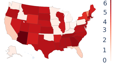
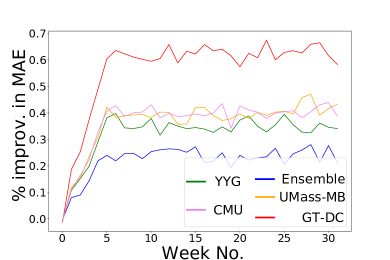
(a) Average % decrease of MAE	(b) % improve. in MAE for each week

Figure 6: (a) B2F refines Ensemble predictions significantly for most states. (b) efficacy of B2F ramps up within 6 weeks of revision data.

B2F also improves Ensemble, which is the current best-performing model of the hub, by 3.6% - 5.18% with over 5% improvement in 38 states, and with IL and TX experiencing over 15% improvement.

Rectifying real-time model-evaluation: We evaluate the efficacy of B2F in rectifying the real-time evaluation scores for the Lbrp problem. We noted in Obs 5 that real-time MAE was lower than stable MAE by 9.6 on average. The difference between B2F rectified estimates MAE stable MAE was reduced to 4.4, a 51.7% decrease (Figure 7). This results in increased MAE scores across most regions towards stable estimates. Eg: We reduce the MAE difference in large highly populated states such as GA by 26.1% (from 22.52 to 16.64) and TX by 90% (from 10.8 to 1.04) causing an increase in MAE scores from real-time estimates by 5.88 and 9.4 respectively.

Refinement as a function of data availability: Note that during the initial weeks of the pandemic, we have access to very little revision data both in terms of length and number of BSeq. So we evaluate the mean performance improvement for each week across all regions (Figure 6b). B2F’s performance ramps up and quickly stabilize in just 6 weeks. Since signals need around 4 weeks (Obs 2) to stabilize, this ramp-up time is impressive. Thus, B2F needs a small amount of revision data to improve model performance.

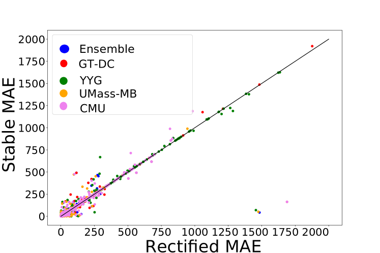
Figure 7: B2F rectified MAE are closer to stable MAE

B2F adapts to anomalies During real-time forecasting, models need to be robust to anomalous data revisions. This is especially true during the initial stages of the pandemic when data collection is not fully streamlined and may experience large revisions. Consider observation week 5 (first week of June) where there was an abnormally large revision to deaths nationwide (Figure 8a) when the BErr was 48%. B2F still provided significant improvements for most model predictions (Figure 8b). Specifically, Ensemble’s predictions are refined to be up to 74.2% closer to stable target.

B2F refines GDP forecasts To evaluate the extensibility of B2F to other domains that encounter the problem of backfill, we tested on the task of forecasting US National GDP at 1 and 2 quarters into the future using 25 macroeconomic indicators from past and their revision history for years 2000-2021. We found that B2F improves predictions of candidate models by 6%-15% and significantly outperforms baselines. The details of the dataset and results are found in Appendix Sections B, E.2.

5 Conclusion

We introduced and studied the challenging multi-variate backfill problem using COVID-19 and GDP forecasting as examples. We presented Back2Future (B2F), the novel deep-learning method to model this phenomenon, which exploits our observations of cross-signal similarities using Graph Recurrent Neural Networks to refine predictions and rectify evaluations for a wide range of models. Our extensive experiments showed that leveraging similarity among backfill patterns via our proposed method leads to impressive 6 - 11 % improvements in all the top models.

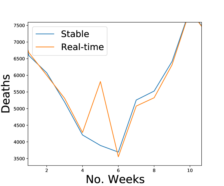
(a) Revision of US deaths on week 5

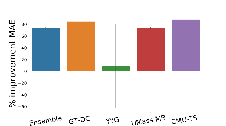
(b) % decrease in MAE due to B2F refinement on week 5 targets

Figure 8: B2F adapts to abnormally high revisions

As future work, our work can potentially help improve data collection and alleviate systematic differences in reporting capabilities across regions. We emphasize that we used the CoVDS dataset as is, but our characterization can be helpful for anomaly detection (Homayouni et al., 2021). We can also study how backfill can affect uncertainty calibration in time-series analysis (Yoon et al., 2020). Adapting to situations where revision history is not temporally uniform across all features due to revisions of different frequency is another research direction.

6 Ethics Statement

Although the features used in the CoVDS dataset and for GDP forecasting are publicly available and anonymized without any sensitive information. However, due to the relevance of our dataset to public health and macroeconomics, prospects for misuse should not be discounted. The disparities in data collection across features and regions can also have implications on equity of prediction performance and is an interesting direction of research. Our backfill refinement framework and B2F is generalizable to any domain that deals with real-time prediction tasks with feature revisions. Therefore, there might be limited potential for misuse of our methods as well.

7 Reproduciblity Statement

As described in Section 4, we evaluated our model over 5 runs with different random seeds to show the robustness of our results to randomization. We also provide a more extensive description of hyperparameters and data pre-processing in the Appendix. The code for B2F and the CoVDS dataset is attached in the appendix. The dataset for GDP Forecasting is publicly available as described in Appendix Section B. Please refer to the README file in the code folder for more details to reproduce the results. On acceptance, we will also make the code and datasets available publicly to encourage reproducibility and allow for further exploration and research.

8 Acknowledgements

This work was supported in part by the NSF (Expeditions CCF-1918770, CAREER IIS-2028586, RAPID IIS-2027862, Medium IIS-1955883, Medium IIS-2106961, CCF-2115126), CDC MInD program, ORNL, and faculty research awards from Facebook, funds/computing resources from Georgia Tech.

Appendix for Back2Future: Leveraging Backfill Dynamics for Improving Real-time Predictions in Future

Code for B2F and the CoVDS dataset is publicly available. Please refer to the README in the code folder for more details to reproduce the results.

Appendix A Additional Related work

Epidemic forecasting. Broadly two classes of approaches have been devised: traditional mechanistic epidemiological models Shaman & Karspeck (2012); Zhang et al. (2017), and the fairly newer statistical approaches Brooks et al. (2018); Adhikari et al. (2019); Osthus et al. (2019b), which have become among the top performing ones for multiple forecasting tasks Reich et al. (2019).

Statistical models have been helpful in using digital indicators such as search queries Ginsberg et al. (2009); Yang et al. (2015) and social media Culotta (2010); Lampos et al. (2010), that can give more lead time than traditional surveillance methods. Recently, deep learning models have seen much work. They can use heterogeneous and multimodal data and extract richer representations, including for modeling spatio-temporal dynamics Adhikari et al. (2019); Deng et al. (2020) and transfer learning Panagopoulos et al. (2021); Rodríguez et al. (2021a). Our work can be thought of refining any model (mechanistic/statistical) in this space.

Revisions and backfill. The topic of revisions has not received as much attention, with few exceptions. In epidemic forecasting, a few papers have mentioned about the ‘backfill problem’ and its effects on performance (Chakraborty et al., 2018; Rodríguez et al., 2021b; Altieri et al., 2021; Rangarajan et al., 2019) and evaluation (Reich et al., 2019); Some works proposed to address the problem via simple models like linear regression (Chakraborty et al., 2014) or ’backcasting’ (Brooks et al., 2018) the observed targets. However they focus only on revisions in the target, and study only in context of influenza forecasting, which is substantially less noisy and more regular than forecasting for the novel COVID-19 pandemic. Reich et al. (2019) proposed a framework to study how backfill affects the evaluation of multiple models, but it is limited to label backfill and flu forecasting. Other works use data assimilation and sensor fusion by leveraging revision free digital signals to refine noisy features for nowcasting (Hawryluk et al., 2021; Farrow, 2016; Lampos et al., 2015; Nunes et al., 2013; Osthus et al., 2019a). However, we observed significant backfill in digital signals as well for COVID-19. Moreover, our model doesn’t require revision-free data sources. Some works model revision of event-based features as count variables which can’t be applicable to many important features like mobility, exposure (Stoner & Economou, 2020; Lawless, 1994). Clements & Galvão (2019) surveys several domain-specific (Carriero et al., 2015) or essentially linear techniques in economics for data revision/correction behavior of the source of several macroeconomic indicators (Croushore, 2011). In contrast, we study the more challenging problem of multi-variate backfill for both features and targets and show how to leverage our insights for more general neural framework to improve both model predictions and evaluation.

Appendix B Details about GDP prediction task

B.1 Dataset

We curated the dataset collected from the Real-Time Data Research Center, Federal Reserve Bank Philadelphia which can be accessed publicly . We extracted the following important macroeconomic features denoted by tickers in parenthesis: Real GDP (ROUTPUT), Real Personal Consumption Expenditures Goods and Services(RCON, RCONG, RCONS), Real Gross Private Domestic Investment (RINVBF, RINVRESID), Real net Exports (RNX), Total Government Consumption (RG, RGF, RGSL), Household Consumption Expenditure (RCONHH), Final Consumption Expenditure (NCON), Nominal GDP (NOUTPUT), Nominal Personal Consumption Expenditures (NCON), Wage and Salary Disbursement (WSD), Other labor Income (OLI), Rental Income (RENTI), Dividends (DIV), Personal Income (PINTI), Transfer Payments (TRANR), Personal Saving Rate (RATESAV), Disposable Personal Income (NDPI), Unemployment Rate (RUC), Civilian Labor Force (LFC), Consumer Price Index (CPI).

B.2 Setup

For each of these 25 features, quarterly data is available since 1965 to third quarter of 2021 and the data is revised quarterly towards more accurate values. Our goal is to predict the Real GDP (ROUTPUT) $k$ quarters ahead using real-time data (data available till current quarter including past data revised till current quarter) where $k\in\{1,2\}$. We tune the hyperparameters for model for using data from years 1995-2000 and test on the unseen period of 2000-2021. Due to lack of standard baselines, we chose as candidate models 1. Vector Autoregression (VAR) model, a standard model in macroeconmics literature (Robertson & Tallman, 1999; Rünstler & Sédillot, 2003; Baffigi et al., 2004), 2. 4-layer feed forward network (FFN) on current quarter’s features similar to (Tkacz & Hu, 1999) and a Recurrent Neural Network (GRU) on past GDP values.

Appendix C Nature of backfill dynamics (More details)

C.1 Considering Delay in reporting

Let current week be $t$. Due to delay in reporting, the first observed value for some signals could be delayed by 1 to 3 weeks. For instance, $\textsc{BSeq}(i,t)$ may not have the first $\delta_{i}$ values due to $\delta_{i}$ weeks delay in reporting. In such cases, for analysis of BSeq in Section 2, we take $d_{i,t}^{t+\delta_{i}}$ as the first value of $\textsc{BSeq}(i,t)=\langle d_{i,t}^{t+\delta_{i}},d_{i,t}^{t+\delta_{i}+1},\cdots,d_{i,t}^{t_{f}}\rangle$. Subsequently, $\textsc{BErr}(r,i,t)$ is only defined for $r>\delta_{i}$ as $\textsc{BErr}(r,i,t)=\frac{|d_{i,t}^{(t+r)}-d_{i,t}^{t_{f}}|}{|d_{i,t}^{t_{f}}|}$.

Real-time forecasting

As mentioned in the main paper, we handle delays in reporting real-time data by approximating from the previous week. During real-time forecasting, we cannot wait for $\delta_{i}$ weeks to get the first value of a signal. Therefore, we replace $d_{i,t}^{(t)}$ with the most revised value of last week for which the signal is available. Let $t^{\prime}<t$ is the last week before $t$ for which we have $d_{i,t^{\prime}}^{(t)}$. Then, we use $d_{i,t^{\prime}}^{(t)}$ in place of unavailable $d_{i,t}^{(t)}$. Note that such cases of missing initial value during real-time forecasting is very uncommon.

C.2 Description of canonical backfill behaviours

We saw in Observation 3 that clustering BSeqs resulted in 5 canonical behaviours. The behaviors of these clusters as shown in Figure 2 can be described as:

Early Decrease: BSeq values stabilizes quickly (within a week) to a lower stable value.

Early Increase: BSeq values increase in 2 to 5 weeks and stabilize.

Steady/Spike: BSeq values either remain constant (no significant revision) or due to reporting errors there may be anomalous values in between. (E.g., for a particular week in the middle of BSeq the signals are revised to 0 due to reporting error).

Late Increase: BSeq values increase and stabilize very late during revision.

Mid Decrease: BSeq values change and stabilize after 8 to 10 weeks of revision.

Table 3: Pearson Correlation Coefficient (PCC) between BErr and RevDiffMAE using stable labels over real-time labels

Model	PCC
Ensemble	-0.327
GT-DC	-0.322
YYG	0.110
UMass-MB	-0.291
CMU-TS	-0.468

C.3 Correlation between BErr and model performance

In Observation 4, we found that models differ in how their performance is impacted by BErr on the label and found that relationship between BErr and difference in MAE (RevDiffMAE) was varied across models with some models (YYG) even showing positive correlation between BErr and RevDiffMAE. To further study this relationship between BErr and reduction in MAE on using stable labels for evaluation over real-time labels by computing the Pearson correlation coefficient (PCC) between BErr and RevDiffMAE for in Table 3. As seen from Figure 3, we observe that for YYG, PCC is positive, indicating that YYG’s scores are actually due to larger BErr on labels. We also see significant differences in PCC for YYG and CMU-TS in over other models.

Appendix D Hyperparameters

In this section, we describe in detail hyperparameters related to data preprocessing and B2F architecture.

D.1 Data Pre-processing

Missing real-time data

Sometimes there is a delay in receiving signals for the current week. In this case, we use values from the most revised version of last observation week for real-time forecasting.

Missing revisions

Once we start observing a signal $d_{t}^{(t)}$ from week $t$ till $t_{f}$, there are weeks $t^{\prime}$ in between where the revised value of this signals is not available or value received is zero. This gives rise to Spike behaviour (Figure 2). Before training, we replace this value with the previous value of BSeq.

Termination of revisions

We observed that for some digital signals, revisions stop a few months in the future. This could be due to the termination of data correction for that signal for older observation weeks. In such cases, we assume that signals are stabilized and use the last available revised values to fill the following values of BSeq.

Scaling signal values

Since each signal that is received has a very different range of values, we rescale each signal with a mean 0. and standard deviation 1.0. Note that since B2F is trained separately for each week, we normalize the data for each week before training.

D.2 Architecture

BseqEnc

The dimension size of all latent encodings $h_{i,t^{\prime}}^{(t^{\prime}_{r})}$ and $v_{i,t^{\prime}}^{(t^{\prime}_{r})}$ is set to 50. Each $GConv$ is a single layer of graph convolutional neural network with weight matrix of size $\mathrm{R}^{50\times 50}$.

ModelPredEnc

For $GRU_{ME}$ We use a GRU of a single hidden layer with output size 50.

Refiner

the feed-forward network $FFN_{RF}$is a 2 layer network with hidden layers of size 60 and 30 followed by final layer outputting 1-dimensional scalar.

Training hyperparameters

We used a learning rate of $10^{-3}$ for pre-training and $5\times 10^{-4}$ for fine-tuning. The pretraining task usually around takes 2000 epoch to train with the first 1000 epochs using teacher forcing and each of the rest of the epoch using teacher forcing with a probability of 0.5. Fine-tuning takes between 500 to 1000 epoch depending on the model, region, and week of the forecast.

As mentioned in Section 4, we used data from June 2020 to Dec 2020 for model design using Observations from Section 2. The hyperparameter tuning was done using data from June 2020 to Aug 2020 and evaluated for time period of Jan 2021 to July 2021. Overall, we found that most hyperparameters are not sensitive. The most sensitive ones mentioned in the main paper are $c\in\{2,3,4,5\}$ that controls sparsity of graph $G_{t}$ and $l=5$ that controls how many steps we auto-regress using BseqEnc to derive latent encodings for BSeq during inference.

Appendix E Additional Results

E.1 COVID-19 Forecasting

We show the average % improvements of all baselines and B2F in Table 4 including for $k=1,3$ week ahead forecasts (We show for $k=2,4$ in main paper Table 2 as well). We show the results for the both June 2020 to Dec 2020 data, which was observed during model design and Jan 2021 to June 2021 which was unseen. B2F show similar performance for both time periods. B2F clearly outperforms all baselines and provides similar improvements for COVID-19 Forecast Hub models for $k=1$ week ahead forecasts as described in Section 4 for other values of $k$.

Table 4: % improvement in MAE and MAPE scores averaged over all regions from June 2020 to Dec 2020

		k=1		k=2		k=3		k=4
Cand. Model	Refining Model	MAE	MAPE	MAE	MAPE	MAE	MAPE	MAE	MAPE
Ensemble	FFNReg	-0.21	-0.45	-0.35	-0.12	0.48	-0.29	0.81	0.36
	PredRNN	-1.67	-0.61	-2.23	-1.57	-1.51	-3.78	-1.13	-2.36
	BseqReg2	0.15	0.19	-1.45	-2.73	-1.74	-3.21	-5.2	-4.78
	BseqReg	2.1	0.29	1.42	0.37	0.37	0.22	0.72	0.28
	B2F	6.22	6.13	5.18	5.47	3.64	3.9	3.61	6.3
GT-DC	FFNReg	-1.92	-1.45	-2.42	-1.51	-2.04	-6.07	-1.86	-0.49
	PredRNN	-3.9	-4.44	-3.02	-3.41	-2.62	-3.95	-2.81	-3.26
	BseqReg2	0.51	0.46	2.24	3.51	2.31	2.42	1.6	0.57
	BseqReg	2.92	2.5	2.13	3.84	3.6	3.55	1.42	2.27
	B2F	10.44	12.37	12.68	12.59	11.42	10.67	9.64	8.97
YYG	FFNReg	-3.45	-1.53	-2.08	-1.34	-4.62	-3.89	-1.37	-3.06
	PredRNN	-1.47	-0.92	-3.84	-6.99	-5.57	-4.16	-9.29	-5.81
	BseqReg2	-1.39	-0.59	-1.25	-0.7	-2.57	-3.72	-6.65	-5.45
	BseqReg	-1.98	-1.92	-1.78	-2.26	-1.99	-1.53	-0.61	-0.43
	B2F	10.64	7.74	8.84	5.98	7.04	7.64	6.8	5.27
UMass-MB	FFNReg	-2.37	-2.03	-3.25	-5.74	-2.16	-3.17	-1.44	-4.84
	PredRNN	-3.52	-4.61	-8.2	-7.54	-5.19	-7.82	-5.99	-7.43
	BseqReg2	-1.01	-0.92	-2.16	-1.88	-2.13	-0.67	-2.29	-2.31
	BseqReg	0.92	0.78	1.58	0.86	-1.26	0.45	0.06	0.03
	B2F	4.44	5.31	5.21	4.92	3.25	4.74	3.94	3.49
CMU-TS	FFNReg	-2.22	-4.17	-5.24	-4.93	-2.87	-1.95	-3.19	-6.7
	PredRNN	-6.59	-4.11	-8.17	-8.21	-3.32	-6.3	-3.75	-9.1
	BseqReg2	0.46	0.71	-0.67	-0.57	-0.73	-0.19	-0.38	-0.12
	BseqReg	1.76	2.34	1.46	1.05	2.74	2.47	2.11	2.84
	B2F	7.54	8.22	8.75	10.48	5.84	7.62	6.93	6.28

Table 5: % improvement in MAE and MAPE scores averaged over all regions from Jan 2021 to June 2021

		k=1		k=2		k=3		k=4
Cand. Model	Refining Model	MAE	MAPE	MAE	MAPE	MAE	MAPE	MAE	MAPE
Ensemble	FFNReg	-0.26	-0.55	-0.35	-0.12	0.43	-0.29	0.87	0.77
	PredRNN	-1.75	-0.74	-2.23	-1.57	-1.63	-3.66	-2.19	-2.85
	BseqReg2	0.08	0.27	-1.45	-2.73	-1.42	-3.88	-5.72	-6.72
	BseqReg	1.85	0.28	1.42	0.37	0.65	0.28	0.74	0.44
	B2F	6.31	6.04	5.25	4.39	3.31	4.19	4.41	3.15
GT-DC	FFNReg	-2.66	-1.35	-2.42	-1.51	-1.49	-6.65	-1.54	-0.48
	PredRNN	-3.51	-4.21	-3.02	-3.41	-2.72	-4.61	-2.91	-3.22
	BseqReg2	0.26	0.67	2.24	3.51	2.34	2.54	1.93	0.78
	BseqReg	2.29	2.95	2.13	3.84	2.37	3.52	1.08	2.33
	B2F	9.61	10.2	10.33	11.84	10.79	10.93	9.92	11.27
YYG	FFNReg	-3.62	-1.53	-2.08	-1.34	-4.41	-3.88	-2.64	-3.36
	PredRNN	-1.35	-1.69	-3.84	-6.99	-5.31	-4.6	-8.84	-5.61
	BseqReg2	-1.74	-0.56	-1.25	-0.7	-2.85	-2.31	-6.13	-5.31
	BseqReg	-2.62	-1.84	-1.78	-2.26	-2.67	-1.17	-0.79	-0.62
	B2F	9.52	6.14	8.93	6.32	6.82	7.58	7.32	5.73
UMass-MB	FFNReg	-2.56	-1.44	-3.25	-5.74	-1.46	-2.58	-1.01	-5.28
	PredRNN	-3.88	-3.85	-8.2	-7.54	-5.55	-8.12	-6.49	-7.56
	BseqReg2	-1.83	-0.91	-2.16	-1.88	-2.73	-0.76	-2.15	-2.87
	BseqReg	0.66	0.73	1.58	0.86	-1.12	0.36	0.36	0.96
	B2F	4.51	4.75	5.43	4.66	5.68	4.89	3.32	3.11
CMU-TS	FFNReg	-3.11	-4.46	-5.24	-4.93	-3.52	-2.32	-3.12	-0.65
	PredRNN	-6.81	-5.92	-8.17	-8.21	-3.75	-7.6	-3.72	-6.11
	BseqReg2	0.41	0.85	-0.67	-0.57	-0.73	-0.29	-0.46	-1.77
	BseqReg	1.33	2.46	1.46	1.05	2.17	2.17	2.38	2.26
	B2F	7.54	8.22	7.5	8.04	6.42	8.23	5.73	6.22

E.2 Real-time GDP Forecasting

We also compare performance of B2F with the baselines for GDP forecasting task in Table 6.

Table 6: % improvement in MAE and MAPE scores for GDP Forecasting from 2000 to 2021

		k=1		k=2
Cand. Model	Refining Model	MAE	MAPE	MAE	MAPE
VAR	FFNReg	2.44$\pm$0.66	2.22 $\pm$ 0.40	3.09$\pm$0.39	4.23$\pm$0.24
	PredRNN	4.05$\pm$ 0.32	3.73$\pm$0.13	3.48$\pm$ 0.23	3.04$\pm$0.29
	BseqReg2	3.32$\pm$0.23	2.40$\pm$0.81	3.39$\pm$0.14	2.99$\pm$0.48
	BseqReg	6.36$\pm$0.38	6.11$\pm$0.15	5.54$\pm$0.42	4.95$\pm$0.23
	B2F	15.88 $\pm$ 0.18	15.71$\pm$0.63	14.94$\pm$0.34	10.26$\pm$0.56
FFN	FFNReg	-0.11$\pm$0.48	-0.15$\pm$0.74	0.48$\pm$0.83	0.36$\pm$0.50
	PredRNN	0.28$\pm$0.44	-0.07$\pm$0.13	-0.24$\pm$0.48	-0.23$\pm$0.62
	BseqReg2	2.26$\pm$0.43	1.98$\pm$0.85	2.29$\pm$0.18	2.20$\pm$0.36
	BseqReg	2.85$\pm$0.51	2.55$\pm$0.39	2.39$\pm$0.13	3.77$\pm$0.42
	B2F	6.63 $\pm$ 0.13	7.30$\pm$0.33	6.07$\pm$0.44	6.61$\pm$ 0.52
GRU	FFNReg	-1.13 $\pm$ 0.03	0.82$\pm$0.26	-1.92$\pm$0.42	-0.70$\pm$0.21
	PredRNN	0.83$\pm$0.25	0.65$\pm$0.38	0.99$\pm$0.37	1.02$\pm$0.26
	BseqReg2	0.62$\pm$0.19	1.29$\pm$0.47	0.92$\pm$0.27	1.15$\pm$0.66
	BseqReg	2.15$\pm$0.66	3.04$\pm$0.73	3.78$\pm$0.58	2.51$\pm$0.61
	B2F	7.52$\pm$0.40	7.18$\pm$0.27	7.28$\pm$0.69	7.59$\pm$0.88

References

- Adhikari et al. (2019) Bijaya Adhikari, Xinfeng Xu, Naren Ramakrishnan, and B Aditya Prakash. Epideep: Exploiting embeddings for epidemic forecasting. In Proceedings of the 25th ACM SIGKDD International Conference on Knowledge Discovery & Data Mining, pp. 577–586, 2019.
- Aguiar (2015) Angel Aguiar. Macroeconomic data. 2015.
- Altieri et al. (2021) Nick Altieri, Rebecca L Barter, James Duncan, Raaz Dwivedi, Karl Kumbier, Xiao Li, Robert Netzorg, Briton Park, Chandan Singh, Yan Shuo Tan, Tiffany Tang, Yu Wang, Chao Zhang, and Bin Yu. Curating a covid-19 data repository and forecasting county-level death counts in the united states. Harvard Data Science Review, 2 2021. doi: 10.1162/99608f92.1d4e0dae. URL https://hdsr.mitpress.mit.edu/pub/p6isyf0g. https://hdsr.mitpress.mit.edu/pub/p6isyf0g.
- Apple (2020) Apple. Apple mobility trends reports., 2020. URL www.apple.com/covid19/mobility.
- Arik et al. (2020) Sercan Arik, Chun-Liang Li, Jinsung Yoon, Rajarishi Sinha, Arkady Epshteyn, Long Le, Vikas Menon, Shashank Singh, Leyou Zhang, Martin Nikoltchev, et al. Interpretable sequence learning for covid-19 forecasting. Advances in Neural Information Processing Systems, 33, 2020.
- Baffigi et al. (2004) Alberto Baffigi, Roberto Golinelli, and Giuseppe Parigi. Bridge models to forecast the euro area gdp. International Journal of forecasting, 20(3):447–460, 2004.
- Biggerstaff et al. (2018) Matthew Biggerstaff, Michael Johansson, David Alper, Logan C Brooks, Prithwish Chakraborty, David C Farrow, Sangwon Hyun, Sasikiran Kandula, Craig McGowan, Naren Ramakrishnan, et al. Results from the second year of a collaborative effort to forecast influenza seasons in the united states. Epidemics, 24:26–33, 2018.
- Brooks et al. (2018) Logan C. Brooks, David C. Farrow, Sangwon Hyun, Ryan J. Tibshirani, and Roni Rosenfeld. Nonmechanistic forecasts of seasonal influenza with iterative one-week-ahead distributions. PLOS Computational Biology, 14(6):e1006134, June 2018. ISSN 1553-7358. doi: 10.1371/journal.pcbi.1006134. URL https://dx.plos.org/10.1371/journal.pcbi.1006134.
- Carriero et al. (2015) Andrea Carriero, Michael P Clements, and Ana Beatriz Galvão. Forecasting with bayesian multivariate vintage-based vars. International Journal of Forecasting, 31(3):757–768, 2015.
- CDC (2020) CDC. Coronavirus Disease 2019 (COVID-19), 2020. URL https://www.cdc.gov/coronavirus/2019-ncov/cases-updates/.
- Chakraborty et al. (2014) Prithwish Chakraborty, Pejman Khadivi, Bryan Lewis, Aravindan Mahendiran, Jiangzhuo Chen, Patrick Butler, Elaine O Nsoesie, Sumiko R Mekaru, John S Brownstein, Madhav V Marathe, et al. Forecasting a moving target: Ensemble models for ili case count predictions. In Proceedings of the 2014 SIAM international conference on data mining, pp. 262–270. SIAM, 2014.
- Chakraborty et al. (2018) Prithwish Chakraborty, Bryan Lewis, Stephen Eubank, John S. Brownstein, Madhav Marathe, and Naren Ramakrishnan. What to know before forecasting the flu. PLoS Computational Biology, 14(10), October 2018. ISSN 1553-734X. doi: 10.1371/journal.pcbi.1005964. URL https://www.ncbi.nlm.nih.gov/pmc/articles/PMC6193572/.
- Chevalier et al. (2021) Judith A Chevalier, Jason L Schwartz, Yihua Su, Kevin R Williams, et al. Measuring movement and social contact with smartphone data: A real-time application to covid-19. Technical report, Cowles Foundation for Research in Economics, Yale University, 2021.
- Cho et al. (2014) Kyunghyun Cho, B. V. Merrienboer, Dzmitry Bahdanau, and Yoshua Bengio. On the properties of neural machine translation: Encoder-decoder approaches. ArXiv, abs/1409.1259, 2014.
- Clements & Galvão (2019) Michael P Clements and Ana Beatriz Galvão. Data revisions and real-time forecasting. In Oxford Research Encyclopedia of Economics and Finance. 2019.
- COVID-Tracking (2020) COVID-Tracking. The covid tracking project., 2020. URL https://covidtracking.com.
- Cramer et al. (2021) Estee Y Cramer, Velma K Lopez, Jarad Niemi, Glover E George, Jeffrey C Cegan, Ian D Dettwiller, William P England, Matthew W Farthing, Robert H Hunter, Brandon Lafferty, et al. Evaluation of individual and ensemble probabilistic forecasts of covid-19 mortality in the us. medRxiv, 2021.
- Croushore (2011) Dean Croushore. Forecasting with real-time data vintages. The Oxford handbook of economic forecasting, pp. 247–267, 2011.
- Culotta (2010) Aron Culotta. Towards detecting influenza epidemics by analyzing twitter messages. In Proceedings of the first workshop on social media analytics, pp. 115–122, 2010.
- Deng et al. (2020) Songgaojun Deng, Shusen Wang, Huzefa Rangwala, Lijing Wang, and Yue Ning. Cola-gnn: Cross-location attention based graph neural networks for long-term ili prediction. In Proceedings of the 29th ACM International Conference on Information & Knowledge Management, pp. 245–254, 2020.
- Devlin et al. (2019) J. Devlin, Ming-Wei Chang, Kenton Lee, and Kristina Toutanova. Bert: Pre-training of deep bidirectional transformers for language understanding. In NAACL-HLT, 2019.
- Farrow (2016) David Farrow. Modeling the past, present, and future of influenza. Private Communication, Farrow’s work will be part of the published Phd thesis at Carnegie Mellon University, 2016.
- Ginsberg et al. (2009) Jeremy Ginsberg, Matthew H Mohebbi, Rajan S Patel, Lynnette Brammer, Mark S Smolinski, and Larry Brilliant. Detecting influenza epidemics using search engine query data. Nature, 457(7232):1012–1014, 2009.
- Google (2020) Google. Google covid-19 community mobility reports., 2020. URL https://www.google.com/covid19/mobility/.
- Hawryluk et al. (2021) Iwona Hawryluk, Henrique Hoeltgebaum, Swapnil Mishra, Xenia Miscouridou, Ricardo P Schnekenberg, Charles Whittaker, Michaela Vollmer, Seth Flaxman, Samir Bhatt, and Thomas A Mellan. Gaussian process nowcasting: Application to covid-19 mortality reporting. arXiv preprint arXiv:2102.11249, 2021.
- Holmdahl & Buckee (2020) Inga Holmdahl and Caroline Buckee. Wrong but Useful — What Covid-19 Epidemiologic Models Can and Cannot Tell Us. NEJM, 383(4):303–305, 2020.
- Homayouni et al. (2021) Hajar Homayouni, Indrakshi Ray, Sudipto Ghosh, Shlok Gondalia, and Michael G Kahn. Anomaly detection in covid-19 time-series data. SN Computer Science, 2(4):1–17, 2021.
- Jin et al. (2020) Xiaoyong Jin, Yu-Xiang Wang, and Xifeng Yan. Inter-series attention model for covid-19 forecasting. ArXiv, abs/2010.13006, 2020.
- Kipf & Welling (2016) Thomas N Kipf and Max Welling. Semi-supervised classification with graph convolutional networks. arXiv preprint arXiv:1609.02907, 2016.
- Lampos et al. (2010) Vasileios Lampos, Tijl De Bie, and Nello Cristianini. Flu detector-tracking epidemics on twitter. In Joint European conference on machine learning and knowledge discovery in databases, pp. 599–602. Springer, 2010.
- Lampos et al. (2015) Vasileios Lampos, Andrew C Miller, Steve Crossan, and Christian Stefansen. Advances in nowcasting influenza-like illness rates using search query logs. Scientific reports, 5(1):1–10, 2015.
- Lawless (1994) JF Lawless. Adjustments for reporting delays and the prediction of occurred but not reported events. Canadian Journal of Statistics, 22(1):15–31, 1994.
- Liu et al. (2017) Shenghua Liu, Bryan Hooi, and Christos Faloutsos. Holoscope: Topology-and-spike aware fraud detection. In Proceedings of the 2017 ACM on Conference on Information and Knowledge Management, pp. 1539–1548, 2017.
- Marcellino (2008) Massimiliano Marcellino. A linear benchmark for forecasting gdp growth and inflation? Journal of Forecasting, 27(4):305–340, 2008.
- Metcalf & Lessler (2017) C Jessica E Metcalf and Justin Lessler. Opportunities and challenges in modeling emerging infectious diseases. Science, 357(6347):149–152, 2017.
- Nunes et al. (2013) Baltazar Nunes, Isabel Natário, and M Lucília Carvalho. Nowcasting influenza epidemics using non-homogeneous hidden markov models. Statistics in Medicine, 32(15):2643–2660, 2013.
- Osthus et al. (2019a) Dave Osthus, Ashlynn R Daughton, and Reid Priedhorsky. Even a good influenza forecasting model can benefit from internet-based nowcasts, but those benefits are limited. PLoS computational biology, 15(2):e1006599, 2019a.
- Osthus et al. (2019b) Dave Osthus, James Gattiker, Reid Priedhorsky, Sara Y Del Valle, et al. Dynamic bayesian influenza forecasting in the united states with hierarchical discrepancy (with discussion). Bayesian Analysis, 14(1):261–312, 2019b.
- Panagopoulos et al. (2020) G. Panagopoulos, Giannis Nikolentzos, and M. Vazirgiannis. United we stand: Transfer graph neural networks for pandemic forecasting. ArXiv, abs/2009.08388, 2020.
- Panagopoulos et al. (2021) George Panagopoulos, Giannis Nikolentzos, and Michalis Vazirgiannis. Transfer graph neural networks for pandemic forecasting. In Proceedings of the AAAI Conference on Artificial Intelligence, 2021.
- Radford et al. (2018) Alec Radford, Karthik Narasimhan, Tim Salimans, and Ilya Sutskever. Improving language understanding with unsupervised learning. 2018.
- Rangarajan et al. (2019) Prashant Rangarajan, Sandeep K Mody, and Madhav Marathe. Forecasting dengue and influenza incidences using a sparse representation of google trends, electronic health records, and time series data. PLoS computational biology, 15(11):e1007518, 2019.
- Reich et al. (2019) Nicholas G. Reich, Logan C. Brooks, Spencer J. Fox, Sasikiran Kandula, Craig J. McGowan, Evan Moore, Dave Osthus, Evan L. Ray, Abhinav Tushar, Teresa K. Yamana, Matthew Biggerstaff, Michael A. Johansson, Roni Rosenfeld, and Jeffrey Shaman. A collaborative multiyear, multimodel assessment of seasonal influenza forecasting in the United States. Proceedings of the National Academy of Sciences of the United States of America, 116(8):3146–3154, 2019. ISSN 1091-6490. doi: 10.1073/pnas.1812594116.
- Robertson & Tallman (1999) John C Robertson and Ellis W Tallman. Vector autoregressions: forecasting and reality. Economic Review-Federal Reserve Bank of Atlanta, 84(1):4, 1999.
- Rodríguez et al. (2021a) Alexander Rodríguez, Nikhil Muralidhar, Bijaya Adhikari, Anika Tabassum, Naren Ramakrishnan, and B Aditya Prakash. Steering a historical disease forecasting model under a pandemic: Case of flu and COVID-19. In Proceedings of the AAAI Conference on Artificial Intelligence, 2021a.
- Rodríguez et al. (2021b) Alexander Rodríguez, Anika Tabassum, Jiaming Cui, Jiajia Xie, Javen Ho, Pulak Agarwal, Bijaya Adhikari, and B. Aditya Prakash. DeepCOVID: An Operational Deep Learning-Driven Framework for Explainable Real-Time COVID-19 Forecasting. In Proceedings of the AAAI Conference on Artificial Intelligence, 2021b.
- Rünstler & Sédillot (2003) Gerhard Rünstler and Franck Sédillot. Short-term estimates of euro area real gdp by means of monthly data. Technical report, ECB working paper, 2003.
- Shaman & Karspeck (2012) Jeffrey Shaman and Alicia Karspeck. Forecasting seasonal outbreaks of influenza. Proceedings of the National Academy of Sciences, 109(50):20425–20430, 2012.
- Stierholz (2017) Katrina Stierholz. Economic data revisions: What they are and where to find them. DttP, 45:4, 2017.
- Stoner & Economou (2020) Oliver Stoner and Theo Economou. Multivariate hierarchical frameworks for modeling delayed reporting in count data. Biometrics, 76(3):789–798, 2020.
- Sutskever et al. (2014) Ilya Sutskever, Oriol Vinyals, and Quoc V. Le. Sequence to sequence learning with neural networks. In NIPS, 2014.
- Tkacz & Hu (1999) Greg Tkacz and Sarah Hu. Forecasting gdp growth using artificial neural networks. Technical report, Bank of Canada, 1999.
- Vaswani et al. (2017) Ashish Vaswani, Noam M. Shazeer, Niki Parmar, Jakob Uszkoreit, Llion Jones, Aidan N. Gomez, Lukasz Kaiser, and Illia Polosukhin. Attention is all you need. ArXiv, abs/1706.03762, 2017.
- Wang et al. (2020) Peng-Wei Wang, Wei-Hsin Lu, Nai-Ying Ko, Yi-Lung Chen, Dian-Jeng Li, Yu-Ping Chang, and Cheng-Fang Yen. Covid-19-related information sources and the relationship with confidence in people coping with covid-19: Facebook survey study in taiwan. Journal of medical Internet research, 22(6):e20021, 2020.
- Yang et al. (2015) Shihao Yang, Mauricio Santillana, and Samuel C Kou. Accurate estimation of influenza epidemics using google search data via argo. Proceedings of the National Academy of Sciences, 112(47):14473–14478, 2015.
- Yin et al. (2020) Changchang Yin, Ruoqi Liu, Dongdong Zhang, and Ping Zhang. Identifying sepsis subphenotypes via time-aware multi-modal auto-encoder. In Proceedings of the 26th ACM SIGKDD international conference on knowledge discovery & data mining, pp. 862–872, 2020.
- Yoon et al. (2020) Jaesik Yoon, Gautam Singh, and Sungjin Ahn. Robustifying sequential neural processes. In Hal Daumé III and Aarti Singh (eds.), Proceedings of the 37th International Conference on Machine Learning, volume 119 of Proceedings of Machine Learning Research, pp. 10861–10870. PMLR, 13–18 Jul 2020. URL http://proceedings.mlr.press/v119/yoon20c.html.
- Zhang et al. (2017) Qian Zhang, Nicola Perra, Daniela Perrotta, Michele Tizzoni, Daniela Paolotti, and Alessandro Vespignani. Forecasting seasonal influenza fusing digital indicators and a mechanistic disease model. In Proceedings of the 26th International Conference on World Wide Web, pp. 311–319. International World Wide Web Conferences Steering Committee, 2017.
- Žliobaite (2010) Indre Žliobaite. Change with delayed labeling: When is it detectable? In 2010 IEEE International Conference on Data Mining Workshops, pp. 843–850. IEEE, 2010.