Abstract

Causal discovery algorithms aim at untangling complex causal relationships from data. Here, we study causal discovery and inference methods based on staged tree models, which can represent complex and asymmetric causal relationships between categorical variables. We provide a first graphical representation of the equivalence class of a staged tree, by looking only at a specific subset of its underlying independences. We further define a new pre-metric, inspired by the widely used structural intervention distance, to quantify the closeness between two staged trees in terms of their corresponding causal inference statements. A simulation study highlights the efficacy of staged trees in uncovering complexes, asymmetric causal relationships from data, and real-world data applications illustrate their use in practical causal analysis.

1 INTRODUCTION

One of the major tasks in all areas of science is to uncover causal relationships between variables of interest. Since experimental data is in many cases unavailable, this task often comes down to discover such relationships using observational data only. This is usually referred to as causal discovery. One of the most common approaches in causal discovery, as well as in causal analysis, is to represent causal relationships via directed acyclic graphs (DAGs). If there is an edge pointing from one variable to another in such graphs, then the former is a direct cause of the latter (Pearl, 2009). The literature on causal discovery using DAGs is now extensive (see Glymour et al., 2019, for a review). The most common approaches are the PC-algorithm (Spirtes et al., 2000), greedy equivalence search (Chickering, 2002) and functional causal models (Hoyer et al., 2008).

Although more efficient and scalable causal discovery algorithms are still being developed (e.g., Bhattacharya et al., 2021; Monti et al., 2020), most of the recent literature has focused on continuous random variables only. Attention to causal discovery for observational discrete data has been limited (see e.g. Cai et al., 2018; Cowell and Smith, 2014; Huang et al., 2018; Peters et al., 2010, for exceptions). The aim of this paper is to discuss flexible and powerful causal discovery algorithms for categorical data embedding complex and asymmetric variable relationships and to highlight their efficacy.

Whilst most causal discovery is carried out via DAG models, here we consider staged tree models (Collazo et al., 2018; Smith and Anderson, 2008) which, differently to DAGs, can represent a wide array of asymmetric causal effects between categorical variables. Bayesian MAP structural learning algorithms for this model class have been introduced (Collazo and Smith, 2016; Cowell and Smith, 2014; Freeman and Smith, 2011) as well as score-based ones (Leonelli and Varando, 2022a; Silander and Leong, 2013). A wide selection of score-based algorithms have been implemented in the open-source stagedtreees R package (Carli et al., 2022) and are used henceforth. Other strategies for non-symmetric relationships in DAG have been proposed in the literature. Two main approaches are modeling CPTs with tree structures (Chickering et al., 1997; Boutilier et al., 1996; Pensar et al., 2016) or using labelled graphs (Pensar et al., 2015).

Despite the importance of uncovering causality from data, only one causal discovery algorithm for staged trees has been proposed (Cowell and Smith, 2014). Here we provide a suite of discovery algorithms based on the dynamic programming approach of Silander and Leong (2013), all freely available in the stagedtrees R package. Furthermore, we perform an extensive simulation study to assess their effectiveness, demonstrating that staged trees are extremely powerful in discovering complex dependence structures and in general outperform DAGs for categorical data.

Just as with DAGs, causal discovery with staged trees can be effectively carried out only if coupled with a method to compute the statistical equivalence class of a model (Collazo et al., 2018). However, the construction of this equivalence class has been shown to be extremely challenging (Duarte and Solus, 2021; Görgen and Smith, 2018; Görgen et al., 2018), and no practical implementations are available. Here we provide a first graphical criterion to characterize part of the equivalence class of a staged tree by looking only at its symmetric independences and showcase its use in practice in our data applications. Approaches restricting the types of independences to be considered when studying equivalence have lately become popular also for DAG models (Markham et al., 2022; Textor et al., 2015; Wienöbst and Liskiewicz, 2020). Notice that once a causal staged tree model is chosen, there is a wide array of methods to estimate causal effects (Genewein et al., 2020; Görgen et al., 2015; Thwaites et al., 2010; Thwaites, 2013).

The quality of our routines is investigated by computing a new measure of dissimilarity between causal models tailored to the topology of staged trees and inspired by the widely-used structural intervention distance (SID) (Peters and Bühlmann, 2015) which we henceforth call context-specific intervention discrepancy (CID). Differently from SID which only accounts for symmetric causal relationships, our defined CID can more generally consider the difference between two causal models by accounting for complex, asymmetric dependencies.

Summarizing, our contributions are the following: (i) a first graphical criterion of equivalence in staged trees; (ii) the first causal measure to compare asymmetric causal relationships in both staged trees and DAGs; (iii) a comparative simulation study highlighting the effectiveness of asymmetric causal discovery; (iv) multiple real-world data applications showcasing our methodology in practice. The code with the implemented methods and the simulation experiments is available in the stagedtrees R package (Carli et al., 2022) and in the repository available at https://github.com/gherardovarando/stagedtrees_causal.

2 STAGED TREES

Let $[p]=\{1,\dots,p\}$ and $\bm{X}=(X_{i})_{i\in[p]}$ be categorical random variables with joint mass function $P$ and sample space $\mathbb{X}=\times_{i\in[p]}\mathbb{X}_{i}$. For $A\subset[p]$, we let $\bm{X}_{A}=(X_{i})_{i\in A}$ and $\bm{x}_{A}=(x_{i})_{i\in A}$ where $\bm{x}_{A}\in\mathbb{X}_{A}=\times_{i\in A}\mathbb{X}_{i}$. We also let $\bm{X}_{-A}=(X_{i})_{i\in[p]\setminus A}$.

Let $(V,E)$ be a directed, finite, rooted tree with vertex set $V$, root node $v_{0}$, and edge set $E$. For each $v\in V$, let $E(v)=\{(v,w)\in E\}$ be the set of edges emanating from $v$ and $\mathcal{C}$ be a set of labels.

Definition 1.

An $\bf X$-compatible staged tree is a triple $(V,E,\eta)$, where $(V,E)$ is a rooted directed tree and:

1. $V={v_{0}}\cup\bigcup_{i\in[p]}\mathbb{X}_{[i]}$;

2. For all $v,w\in V$, $(v,w)\in E$ if and only if $w=\bm{x}_{[i]}\in\mathbb{X}_{[i]}$ and $v=\bm{x}_{[i-1]}$, or $v=v_{0}$ and $w=x_{1}$ for some $x_{1}\in\mathbb{X}_{1}$;

3. $\eta:E\rightarrow\mathcal{L}=\mathcal{C}\times\cup_{i\in[p]}\mathbb{X}_{i}$ is a labelling of the edges such that $\eta(v,\bm{x}_{[i]})=(\kappa(v),x_{i})$ for some function $\kappa:V\to\mathcal{C}$.

If $\eta(E(v))=\eta(E(w))$ then $v$ and $w$ are said to be in the same stage.

Therefore, the equivalence classes induced by $\eta(E(v))$ form a partition of the internal vertices of the tree in stages.

Figure 1: An example of an $(X_{1},X_{2},X_{3})$-compatible (left) and an $(X_{1},X_{3},X_{2})$-compatible (right) staged trees.

Definition 1 first constructs a rooted tree where each root-to-leaf path, or equivalently each leaf, is associated with an element of the sample space $\mathbb{X}$. Then a labeling of the edges of such a tree is defined where labels are pairs with one element from a set $\mathcal{C}$ and the other from the sample space $\mathbb{X}_{i}$ of the corresponding variable $X_{i}$ in the tree. By construction, $\bf X$-compatible staged trees are such that two vertices can be in the same stage if and only if they correspond to the same sample space. Although staged trees can be more generally defined without imposing this condition, henceforth, and as common in practice, we focus on $\bf{X}$-compatible staged trees only (see Leonelli, 2019, for an example of a non $\bf{X}$-compatible tree).

Figure 1 (left) reports an $(X_{1},X_{2},X_{3})$-compatible stratified staged tree over three binary variables. The coloring given by the function $\kappa$ is shown in the vertices and each edge $(\cdot,(x_{1},\ldots,x_{i}))$ is labeled with $X_{i}=x_{i}$. The edge labeling $\eta$ can be read from the graph combining the text label and the color of the emanating vertex. The staging of the staged tree in Figure 1 is given by the partition $\{v_{0}\}$, $\{v_{1},v_{2}\}$, $\{v_{3},v_{4}\}$, $\{v_{5}\}$ and $\{v_{6}\}$.

The parameter space associated to an $\bf X$-compatible staged tree $T=(V,E,\eta)$ with labeling $\eta:E\rightarrow\mathcal{L}$ is defined as

$$\Theta_{T}=\Big{\{}\bm{\theta}\in\mathbb{R}^{\eta(E)}\;|\;\forall e\in E,\theta_{\eta(e)}\in(0,1)\textnormal{ and }$$

$$\forall v\in V,\sum_{e\in E(v)}\theta_{\eta(e)}=1\Big{\}}$$

Let $\bm{l}_{T}$ denote the leaves of a staged tree $T$. Given a vertex $v\in V$, there is a unique path in $T$ from the root $v_{0}$ to $v$, denoted as $\lambda(v)$. For any path $\lambda$ in $T$, let $E(\lambda)=\{e\in E:e\in\lambda\}$ denote the set of edges in the path $\lambda$.

Definition 2.

The staged tree model $\mathcal{M}_{T}$ associated to the $\bf X$-compatible staged tree $(V,E,\eta)$ is the image of the map

$$\begin{array}[]{llll}\phi_{T}&:&\Theta_{T}&\to\Delta_{|\bm{l}_{T}|-1}\\ &&\bm{\theta}&\mapsto\Big{(}\prod_{e\in E(\lambda(l))}\theta_{\eta(e)}\Big{)}_{l\in\bm{l}_{T}}\end{array}$$ (1)

An element of $\mathcal{M}_{T}$ in Definition 2 identifies a joint probability $P_{\bm{\theta}}$ with conditional distributions, for all $\bm{x}\in\mathbb{X}$ and $i\in[p]$,

$$P_{\bm{\theta}}(X_{i}=x_{i}|X_{[i-1]}=\bm{x}_{[i-1]})=\theta_{\eta(\bm{x}_{[i-1]},\bm{x}_{[i]})}.$$

Definition 3.

Two staged trees $T$ and $S$ are said to be statistically equivalent if they induce the same models, that is $\mathcal{M}_{T}=\mathcal{M}_{S}$.

2.1 Conditional Independence and graphical representation

A symmetric or total, conditional independence statement, or just conditional independence (CI) ($X_{A}\mathchoice{\mathrel{\hbox to0.0pt{$\displaystyle\perp$\hss}\mkern 2.0mu{\displaystyle\perp}}}{\mathrel{\hbox to0.0pt{$\textstyle\perp$\hss}\mkern 2.0mu{\textstyle\perp}}}{\mathrel{\hbox to0.0pt{$\scriptstyle\perp$\hss}\mkern 2.0mu{\scriptstyle\perp}}}{\mathrel{\hbox to0.0pt{$\scriptscriptstyle\perp$\hss}\mkern 2.0mu{\scriptscriptstyle\perp}}}X_{B}|X_{C}$) holds for a probability distribution $P$, over categorical random variable, if

$$P(X_{A}|X_{B}=x_{B},X_{C}=x_{C})=P(X_{A}|X_{C}=x_{c}),$$ (2)

for every $x_{B}\in\mathbb{X}_{B}$ and $x_{c}\in\mathbb{X}_{C}$. Conditional independence statements can be efficiently represented by DAGs model and the d-separation criterion (Pearl and Verma, 1987; Verma and Pearl, 1990). In particular if a probability distribution $P$ over $X_{1},\ldots,X_{p}$ belongs to the model class associated with a DAG $G$, then $X_{i}\mathchoice{\mathrel{\hbox to0.0pt{$\displaystyle\perp$\hss}\mkern 2.0mu{\displaystyle\perp}}}{\mathrel{\hbox to0.0pt{$\textstyle\perp$\hss}\mkern 2.0mu{\textstyle\perp}}}{\mathrel{\hbox to0.0pt{$\scriptstyle\perp$\hss}\mkern 2.0mu{\scriptstyle\perp}}}{\mathrel{\hbox to0.0pt{$\scriptscriptstyle\perp$\hss}\mkern 2.0mu{\scriptscriptstyle\perp}}}X_{j}|X_{C}$ with respect to $P$ if $i$ and $j$ are d-separated by $C$ in $G$. Thus we can graphically read in $G$ the conditional independence statements that hold for every distribution Markov with respect to $G$.

For categorical random variables, we could envisage those equality relationships such as Equation 2 hold only for a subset of values of $x_{B}$ and/or $x_{C}$. This generalized asymmetric conditional independences can be organized into three classes: (i) Context-specific CI (Boutilier et al., 1996), when $P(X_{A}|X_{B}=x_{B},X_{C}=x_{C})=P(X_{A}|X_{C}=x_{c})$ for all $x_{B}\in\mathbb{X}_{B}$ and for a subset of possible value $x_{C}\in\mathcal{C}\subseteq\mathbb{X}_{C}$ (the context). (ii) Partial CI (Pensar et al., 2016), when $P(X_{A}|X_{B}=x_{B},X_{C}=x_{C})=P(X_{A}|X_{C}=x_{C})$ for a subset of values $x_{B}\in\mathcal{B}\subseteq\mathbb{X}_{B}$ and a subset of values $x_{C}\in\mathcal{C}\subseteq\mathbb{X}_{C}$. (iii) Local CI (Chickering et al., 1997), when $P(X_{A}|X_{C}=x^{1}_{C})=P(X_{A}|X_{C}=x^{2}_{C})$. Such asymmetric CI statements cannot be encoded graphically in a classical DAG model, since they refer to equalities valid in specific conditional probability tables. Previous works have thus modeled such equality relationships by either modeling CPTs with tree structures (Chickering et al., 1997; Boutilier et al., 1996; Pensar et al., 2016) or by considering only context-specific CIs and using labelled DAGs (Pensar et al., 2015).

In the staged tree in Figure 1 (left), we can see how the vertex staging represents conditional independence: the fact that $v_{1}$ and $v_{2}$ are in the same stage (green) implies that $X_{1}\mathchoice{\mathrel{\hbox to0.0pt{$\displaystyle\perp$\hss}\mkern 2.0mu{\displaystyle\perp}}}{\mathrel{\hbox to0.0pt{$\textstyle\perp$\hss}\mkern 2.0mu{\textstyle\perp}}}{\mathrel{\hbox to0.0pt{$\scriptstyle\perp$\hss}\mkern 2.0mu{\scriptstyle\perp}}}{\mathrel{\hbox to0.0pt{$\scriptscriptstyle\perp$\hss}\mkern 2.0mu{\scriptscriptstyle\perp}}}X_{2}$; in fact, from the definition of staged tree model, the context-specific conditional distribution of $X_{2}$ given $X_{1}=0$, represented by the edges emanating from $v_{1}$, is equal to the conditional distribution of $X_{2}$ given $X_{1}=1$. The staging given by the light-blue vertices implies instead the context-specific independence (Boutilier et al., 1996) $X_{3}\mathchoice{\mathrel{\hbox to0.0pt{$\displaystyle\perp$\hss}\mkern 2.0mu{\displaystyle\perp}}}{\mathrel{\hbox to0.0pt{$\textstyle\perp$\hss}\mkern 2.0mu{\textstyle\perp}}}{\mathrel{\hbox to0.0pt{$\scriptstyle\perp$\hss}\mkern 2.0mu{\scriptstyle\perp}}}{\mathrel{\hbox to0.0pt{$\scriptscriptstyle\perp$\hss}\mkern 2.0mu{\scriptscriptstyle\perp}}}X_{2}|X_{1}=0$: the independence between $X_{3}$ and $X_{2}$ holds only for one of the two levels of $X_{1}$. For such a staged tree there is no equivalent DAG representation since it embeds non-symmetric conditional independences (Varando et al., 2021).

In the staged tree in Figure 1 (right), we can observe that the stages structure for the last variable implies the following equalities: $P(X_{2}|X_{1}=0,\,X_{3}=0)=P(X_{2}|X_{1}=1,\,X_{3}=1)$ and $P(X_{2}|X_{1}=0,\,X_{3}=1)=P(X_{2}|X_{1}=1,\,X_{3}=0)$. This is what is defined as a local CI (Chickering et al., 1997), it is a relationship between conditional probabilities which cannot be expressed as traditional conditional independence nor context-specific or partial. We refer to Pensar et al. (2016) and Varando et al. (2021) for additional discussion and examples of asymmetric CIs.

2.2 Staged Trees and DAGs

Consider a DAG $G$ and the associated statistical model $\mathcal{M}_{G}$ of all distributions that are Markov to $G$. Smith and Anderson (2008) showed that one can always construct a staged tree $T_{G}$ such that $\mathcal{M}_{G}=\mathcal{M}_{T_{G}}$. However, given a staged tree $T$ in general one cannot find a DAG $G_{T}$ such that $\mathcal{M}_{T}=\mathcal{M}_{G_{T}}$ since staged trees embed asymmetric independences that DAGs cannot represent.

Varando et al. (2021) demonstrated that it is possible to find a minimal DAG $G_{T}=([p],F)$ such that $\mathcal{M}_{T}\subseteq\mathcal{M}_{G_{T}}$, and this minimal $G_{T}$ represents all symmetric conditional independences of $T$. More formally, $X_{i}\mathchoice{\mathrel{\hbox to0.0pt{$\displaystyle\perp$\hss}\mkern 2.0mu{\displaystyle\perp}}}{\mathrel{\hbox to0.0pt{$\textstyle\perp$\hss}\mkern 2.0mu{\textstyle\perp}}}{\mathrel{\hbox to0.0pt{$\scriptstyle\perp$\hss}\mkern 2.0mu{\scriptstyle\perp}}}{\mathrel{\hbox to0.0pt{$\scriptscriptstyle\perp$\hss}\mkern 2.0mu{\scriptscriptstyle\perp}}}X_{i}|\bm{X}_{C}$ holds in $\mathcal{M}_{T}$ if and only if $i$ and $j$ are d-separated by $C$ in $G_{T}$. For instance, the minimal DAG representation of the staged tree in Figure 1 (left) is the v-structure $1\rightarrow 3\leftarrow 2$.

In Varando et al. (2021) DAGs $G_{T}$ are also extended to have a labeling of their edges according to the type of dependence existing between any pair of random variables in the underlying staged tree $T$ (according to the categorization of asymmetric independence given in Pensar et al., 2016). They termed such labeled DAGs as asymmetry-labeled DAGs (ALDAGs) and introduce algorithms to learn them from data. For the purposes of this paper, we are interested in a simplified version of the labeling; we are, in particular, interested only in identify the subset of edges in $G_{T}$ which cover some asymmetric conditional independence statements.

Definition 4.

Let $G_{T}$ be the minimal DAG of an $\bm{X}$-compatible staged tree $T=(V,E,\eta)$ and an edge $(i,j)$ of $G$ is called non-total if

$$\eta(E(\bm{x}_{[j-1]}))=\eta(E(\bm{x}^{\prime}_{[j-1]})),$$

$$\text{for }\bm{x}_{[j-1]},\bm{x}^{\prime}_{[j-1]}\in\mathbb{X}_{[j-1]},$$

$$\,\text{s.t.}\,{x}_{i}\neq x^{\prime}_{i}.$$

An edge is called total otherwise.

Intuitively an edge $(i,j)$ in a minimal DAG is non-total when the variable $X_{i}$ is “involved” is a non-symmetrical conditional independence for $X_{j}$. The edges of a minimal DAG $G_{T}=([p],F)$ can thus be partitioned in total ($F^{tot}$) and non-total edges ($F^{nt}$).

As an illustration, in the minimal DAG from the tree on the left of Figure 1 ($1\rightarrow 3\leftarrow 2$), the edge $(2,3)$ is non-total because $v_{3}$ and $v_{4}$ belong to the same stage.

2.3 Causal Models Based on Staged Trees

We can define a finite-interventional causal model (Rischel and Weichwald, 2021) induced by a staged tree as a collection of interventional distributions in an intuitive way: the joint distribution of $\bm{x}$ in the intervened model is obtained by the product of the parameters in the corresponding root-to-leaf path where we replace parameters corresponding to intervened variables.

Definition 5.

A staged tree causal model induced by an $\mathbf{X}$-compatible staged tree $T=(V,E,\eta)$ is the class of interventional distributions defined, for each parameter vector $\bm{\theta}\in\Theta_{T}$, as follows:

$$P_{\bm{\theta}}\left(\bm{X}=\bm{x}|\operatorname{do}(\bm{X}_{I}=\bm{z}_{I})\right)=\prod_{i\not\in I}\theta_{\eta(\bm{x}_{[i]},\bm{x}_{[i-1]})}\prod_{i\in I}\delta(x_{k},z_{k})$$ (3)

$$=\left\{\begin{matrix}\frac{P_{\bm{\theta}}(\bm{X}=\bm{x})}{\prod_{i\in I}P_{\bm{\theta}}(X_{i}=x_{i}|\bm{X}_{[i-1]}=\bm{x}_{[i-1]})}&\text{if }\bm{x}_{I}=\bm{z}_{I}\\ 0&\text{otherwise}\end{matrix}\right.$$

In particular, under the empty intervention, we recover the observational distribution $P_{\bm{\theta}}$.

We say that two staged trees $T$ and $S$ are causally equivalent if they induce the same class of interventional distributions as in Definition 5. Obviously, two causally equivalent staged trees are also statistically equivalent but not vice versa.

We have that, as for DAGs, intervening on some variables, only affects downstream variables, for $i\not\in I$ and an $\bm{X}$-compatible staged tree:

$$P_{\bm{\theta}}\left(X_{i}|\operatorname{do}(\bm{X}_{I}=\bm{x}_{I})\right)=P_{\bm{\theta}}\left(X_{i}|\operatorname{do}(\bm{X}_{I^{*}}=\bm{x}_{I^{*}})\right),$$ (4)

$$\text{where }I^{*}=I\cap[i-1]$$

And, in particular,

$$P_{\bm{\theta}}\left(X_{i}=x_{i}|\operatorname{do}(\bm{X}_{[i-1]}=\bm{x}_{[i-1]})\right) =$$

$$P_{\bm{\theta}}\left(X_{i}=x_{i}|\bm{X}_{[i-1]}=\bm{x}_{[i-1]}\right) =\theta_{\eta(\bm{x}_{[i-1]},\bm{x}_{[i]})}.$$

3 CAUSAL DISCOVERY ALGORITHMS

As discussed by Collazo et al. (2018) and Cowell and Smith (2014), causal discovery algorithms for staged trees must combine two routines: (i) an algorithm learning the stage structure of the tree with a fixed variable ordering; (ii) an algorithm exploring the possible variable orderings. Both are reviewed next.

3.1 Learning the Stage Structure with a Fixed Order

The space of possible $\bm{X}$-compatible staged trees is considerably larger than the space of possible DAGs. Even if we fix the order of the variables, exploring all possible combinations of stages structure becomes rapidly infeasible (Collazo et al., 2018). We thus use two of the possible heuristic searches implemented in the stagedtrees package (Carli et al., 2022). In both cases, we use the BIC score as criterion for selecting the best ordering of the variables (see Görgen et al., 2022, for details). However, our implementation can be coupled with any algorithm available in the stagedtrees package.

The backward hill-climbing (BHC) method consists in starting from the saturated model and, for each variable, iteratively trying to join stages. At each step of the algorithm, all possible combinations of two stages are tried and the best move is chosen. Since the log-likelihood decomposes across the depth of the tree, the stages search can be performed independently for each variable.

The use of the k-means clustering of probabilities to learn staged event tree was first introduced by Silander and Leong (2013) as a fast alternative to backward hill-climbing algorithms. The default version implemented in the stagedtrees package performs k-means clustering over the square root of the probabilities of a given variable given all the possible contexts. Both algorithms operate over the stage structures of each variable $X_{i}$ independently of the other variable stages. Furthermore, the estimated stage structure of a given variable depends only on which variables precede $X_{i}$, independently of their order.

3.2 Learning an Optimal Variable Ordering

The methods described in the previous section output an $\bm{X}_{\pi}$-compatible staged tree for a possible ordering $\pi$ of the variables. For a small number of variables, it is possible to simply enumerate all possible $p!$ staged trees for all possible orders, and select the best one(s) according to a chosen criterion (e.g. BIC). Silander and Leong (2013) proposed a dynamic programming algorithm that still obtains a global optimum, but with a substantial reduction in computational complexity. The method can be coupled with every algorithm which operates independently on every variable and using as guiding score any function which can be decomposed across the variables of the model.

3.3 Related Work

In principle, non-symmetric CI statements are represented by equalities in conditional probability tables (CPT) in categorical DAG parametrizations. Still, a classical (or full tables) DAG is not able to represent graphically such asymmetric relationships, in the sense that such equalities are not encoded in any particular structure. A simple extension of DAGs could consider additional nodes representing values of variables (e.g. $X_{1}=0$, $X_{1}=1$) in order to represent context-specific relationships. Unfortunately, this strategy works only for univariate contexts and, it would entail deterministic relationships between some nodes in the DAG (e.g. $X_{1}=0$ and $X_{1}=1$).

More complex strategies for non-symmetric relationships in DAGs have been proposed in the literature. Two main approaches are modeling CPTs with tree structures (Chickering et al., 1997; Boutilier et al., 1996; Pensar et al., 2016) or use labelled graphs (Pensar et al., 2015) for context-sepcific independences. DAGs with tree-parametrized CPTs and staged tree methods are very similar approaches that use trees to represent conditional probabilities. In particular, the statistical models represented by staged tree and DAGs with tree-CPTs are, in principle, equivalent. Even the learning algorithm proposed by Pensar et al. (2016) consist in a heuristic search using splitting and joining operation on each CPT-tree, similar in a way to the hill-climbing moves proposed also for staged trees (Carli et al., 2022). The difference is that, in the staged tree approach, we do not assume a sparse DAG between variables and we do not search both a DAG and sparse CPTs. Of course, restricting to sparse DAG is beneficial from a computational perspective, and it has been proposed and shown to be effective also for staged trees (Barclay et al., 2013; Leonelli and Varando, 2022b). Unfortunately, we are not aware of any available implementation of these related methods and we were thus unable to run any empirical comparisons.

3.4 Exploring the Equivalence Class

Given a learned staged tree from data, any formal causal analysis also needs exploration of the associated statistical equivalence class. For staged trees, this has been shown to be extremely complex. Görgen and Smith (2018) and Görgen et al. (2018) give polynomial criteria which are complex to implement in practice, whilst Duarte and Solus (2021) considers a particular subclass of staged trees. The following proposition paves the way toward the exploration of the equivalence class of a staged tree.

Proposition 1.

Let $T$ be an $\bm{X}$-compatible staged tree and $G_{T}=([p],F=F^{tot}\cup F^{nt})$ its minimal DAG, where we denote with $F^{nt}$ the non-total edges of $G_{T}$. Let $G^{\prime}=([p],F^{\prime}\cup F^{nt})$ be a DAG in the same Markov equivalence class of $G_{T}$, where $\pi$ is one of its topological orders. If additionally $([p],F^{\prime})$ and $([p],F^{tot})$ are Markov equivalent, then there exists an $\bm{X}_{\pi}$-compatible staged tree $S$ (with minimal DAG $G^{\prime}$) such that $\mathcal{M}_{T}=\mathcal{M}_{S}$. Vice versa, If $\mathcal{M}_{T}=\mathcal{M}_{S}$ their minimal DAGs $G_{T}$ and $G_{S}$ are Markov equivalent.

However, there may be equivalent staged trees whose minimal DAGs have “non-total" edges with a different directionality (see e.g. Pensar et al., 2015). As an illustration of Proposition 1, consider the staged tree in Figure 1 (left). Its minimal DAG is the v-structure $X_{1}\rightarrow X_{3}\leftarrow X_{2}$. Therefore there exists, at least, an $(X_{2},X_{1},X_{3})$-compatible staged tree which is statistically equivalent to the one in Figure 1 (left), and there cannot be a statistically equivalent staged tree where $X_{3}$ is not the last variable.

Although Proposition 1 does not give a complete characterization of the equivalence class, it is important because it informs about relationships existing in the staged tree which cannot be interpreted as causal if learned from data. We showcase in Section 6 how the proposition can be used for applied causal analyses.

4 CONTEXT-SPECIFIC INTERVENTIONAL DISCREPANCY

Similarly to the structural interventional distance (SID) for DAGs (Peters and Bühlmann, 2015), which counts the number of wrongly estimated interventional distributions, we can define a context interventional discrepancy, with respect to a reference staged tree ($T$). Such a discrepancy measures the extent of the errors done in computing context-specific interventions using a different staged tree ($S$).

Definition 6.

Let $T=(V,E,\eta)$ be an $\bm{X}$-compatible staged event tree and $S=(W,F,\nu)$ an $\bm{X}_{\pi}$-compatible staged event tree, where $\pi$ is a permutation of $[p]$. We define the context interventional discrepancy $\operatorname{CID}(T,S)$ as,

$$\operatorname{CID}(T,S)=\sum_{i\in[p]}\operatorname{CID}_{i}(T,S),$$

where $\operatorname{CID}_{i}\left(T,S\right)$ is the proportion of contexts $\bm{x}_{[i-1]}\in\mathbb{X}_{[i-1]}$ for which the interventional distribution $P(X_{i}|\operatorname{do}(\bm{X}_{[i-1]}=\bm{x}_{[i-1]}))$ is wrongly inferred by $S$ with respect to $T$. Precisely, we say that $P(X_{i}|\operatorname{do}(\bm{X}_{[i-1]}=\bm{x}_{[i-1]}))$ is wrongly inferred by $S$ with respect to $T$ if there exists $P\in\mathcal{M}_{T}$ such that

$$P(X_{i}|\bm{X}_{[i-1]}=\bm{x}_{[i-1]})\neq\\ P\left(X_{i}|\bm{X}_{I}\in\left\{\begin{matrix}\bm{y}_{I}\in\mathbb{X}_{I}:\nu(E(\bm{y}_{K}))=\nu(E(\bm{x}_{K}))\\ \text{ for some }\bm{y}_{K\setminus I},\bm{x}_{K\setminus I}\in\mathbb{X}_{K\setminus I}\end{matrix}\right\}\right)$$

where $K=\{j:\pi^{-1}(j)<\pi^{-1}(t)\}$ are the variables preceding $X_{i}$ in $S$ and $I=K\cap[i-1]$.

Intuitively, CID measures how much a different staged tree $S$ can be used to compute interventional distributions of the type $P(X_{i}|\operatorname{do}(\bm{X}_{[i-1]}=\bm{x}_{[i-1]}))$. We choose to consider only univariate distributions under interventions on the preceding variables in the true model $T$, instead of pairwise interventional distributions of the form $P(X_{i}|\operatorname{do}(X_{j}=x_{j}))$ as in the definition of SID (Peters and Bühlmann, 2015). This is because our goal is to quantify the effect of context-specific interventions. Moreover, differently from SID, we do not control if the additional variables preceding $X_{i}$ in $S$ are a valid adjustment set. This simplification is taken to avoid the computational complexity of having to check the stages structure for all the variables in the eventual adjustment set. Nevertheless, the proposed CID is a sensitive measure of correctness of the causal model, as Proposition 2 and Figure 2 show. However, other measures of the differences between staged tree causal models could be alternatively defined, eventually considering different intervention classes or validity of the adjustment sets.

The algorithm to compute the context-specific interventional discrepancy is given in the Appendix where its correctness is also proven.

As an example of the computation of CID$(T,S)$, consider the two staged trees in Figure 1, where the left tree is $T$ and the right one is $S$. We need to determine which interventional distributions for the left staged tree are wrongly inferred by the right one. For example, consider the intervention $\operatorname{do}(X_{1}=0,X_{2}=1)$ and the distribution $P(X_{3}|\operatorname{do}(X_{1}=0,X_{2}=1))$ for $P\in\mathcal{M}_{T}$. We have that,

$$P(X_{3}|\operatorname{do}(X_{1}=0,X_{2}=1))=P(X_{3}|X_{1}=0,X_{2}=1),$$

and, $I=\{1\}$, thus, because $v_{3}$ and $v_{4}$ belong to the same stage in $T$:

$$P(X_{3}|X_{1}=0) =P(X_{3}|X_{1}=0,X_{2}=0)$$

$$=P(X_{3}|X_{1}=0,X_{2}=1),$$

and $P(X_{3}|\operatorname{do}(X_{1}=0,X_{2}=1))$ is then correctly inferred by $S$. On the other hand, we have that $P(X_{3}|\operatorname{do}(X_{1}=1,X_{2}=1))$ is wrongly inferred by $S$ because $P(X_{3},|X_{1}=1,X_{2}=1)\neq P(X_{3}|X_{1}=1)$ in general. To see this, notice that

$$P( X_{3}|X_{1}=1)=$$

$$\sum_{x_{2}=0,1}P(X_{3}|X_{1}=1,X_{2}=x_{2})P(X_{2}=x_{2}|X_{1}=1).$$

And $P(X_{3},|X_{1}=1,X_{2}=1)\neq P(X_{3}|X_{1}=1)$ if, for example, we choose $P(X_{2}=x_{2}|X_{1}=1)=0.5$ and $P(X_{3}|X_{1}=1,X_{2}=0)\neq P(X_{3}|X_{1}=1,X_{2}=1)$.

As another example, consider the interventional distribution $P(X_{2}|\operatorname{do}(X_{1}=1))$. In this case we have $I=\{1\}$, and since vertices $v_{1},v_{2}$ are in the same stage (and so are $\{w_{5},w_{4}\}$ and $\{w_{3},w_{6}\}$), we have that

$$P(X_{2}|X_{1}=1)=P(X_{2})=P(X_{2}|X_{1}\in\{0,1\}),$$

that is, $S$ correctly infers the interventional distribution $P(X_{2}|\operatorname{do}(X_{1}=1))$ for every $P\in\mathcal{M}_{T}$.

Similar to SID, the context-specific intervention discrepancy is not symmetric. The following proposition collects some properties of the newly defined measure.

Proposition 2.

The following properties hold for $\operatorname{CID}$.

1. $\operatorname{CID}(T,S)=0$ for every pair of causally equivalent staged trees $S,T$.

2. If $\mathcal{M}(T)\subseteq\mathcal{M}(S)$ and $\pi$ is the identity, then $\operatorname{CID}(T,S)=0$.

3. If $\mathcal{M}_{T}$ is the full independence model then $CID(T,S)=0$ for every $X_{\pi}$-compatible staged tree $S$.

Notice that CID can also be used to compare categorical causal DAGs, since we can always transform a DAG $G$ to its equivalent staged tree representation $T_{G}$. In order to compare CID and SID we perform a simulation study where we sample uniformly DAGs over $5$ binary variables and compute their CID and SID. The results are reported in the two-dimensional density and scatter plot in Figure 2. We can see that there is a high correlation between the two measures thus highlighting that CID is a sensible measure that could be used not only for non-symmetric models but also for symmetric ones based on DAGs.

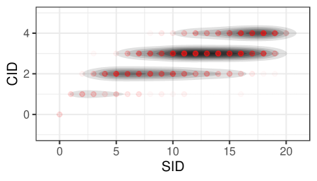
Figure 2: CID and SID between randomly generated DAGs over $5$ binary variables. The correlation between CID and SID is $0.67$ ($95\%$ confidence interval: $(0.633,0.701)$)

.

5 SIMULATION EXPERIMENTS

We perform a simulation study to evaluate the feasibility of the proposed approach and to demonstrate its superiority with respect to the classical DAG algorithms under the assumption that the true model is a staged tree. We simulate data from randomly generated staged tree models with different degrees of complexity: number of stages per variable ($k\in\{2,3,4\}$). We consider models with $3,\ldots,6$ binary variables, and sample sizes ranging from $100$ to $10000$ observations. For each parameters’ combination, we perform $100$ repetition of the experiment each time randomly shuffling the order of the variables to eliminate any possible bias of the search heuristics.

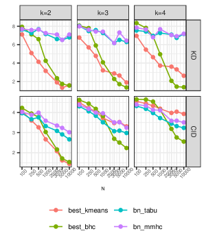
Figure 3: Context interventional discrepancy (CID) and Kendall tau distance (KD) between the estimated and true model.

We run the staged trees approach described in Section 3 using the backward hill-climbing search (best_bhc) and the k-means heuristic (best_kmeans) with the number of clusters fixed to $2$. Our two routines are compared to two classical DAG learning algorithms such as tabu search (tabu) (Russell and Norvig, 2009) and max-min hill-climbing (mmhc) (Tsamardinos et al., 2006), both implemented in the bnlearn R package (Scutari, 2010). Results are displayed in Figure 3, where the average CID and Kendall tau distance between the variable orderings are plotted as a function of the sample size $N$ for the case of $6$ variables. The Kendall tau distance is computed between the true causal order and the estimated order with the implementation in the PerMallows R package (Irurozki et al., 2016).

We can observe that, as expected, methods based on staged trees are able to better recover the causal structure of the true model. Since the true models are randomly generated staged trees we can expect that algorithms which search for the best DAG are not able to recover the true relationships between the variables. More specifically, we observe that the method based on the k-means algorithm works very well when the number of stages per variable matches the number of clusters ($k=2$), while, with respect to CID, its performance degrades for $k=3,4$. The backward hill-climbing method, instead, requires a bigger sample size, but it is able to perform well even when the true model is more complex. Additionally, it is interesting to notice that both staged tree approaches are able to recover well the causal order of the variables in all considered scenarios. This is especially interesting for the k-means algorithm which performs better than the backward hill-climbing method with respect to the Kendall distance even when it is misspecified ($k>2$). In the Supplementary Materials, we report the computational times of the algorithms. As expected, algorithms for DAGs are faster since the searched model space is much smaller. The k-means algorithm for staged trees is comparable to those for DAGs in terms of speed and its complexity does not seem to exponentially increase as in the case of the backward hill-climbing.

6 REAL WORLD EXAMPLES

6.1 ISTAT: Aspects on Everyday Life

We illustrate the use of staged trees to uncover causal relationships using data from the 2014 survey “Aspects on everyday life" collected by ISTAT (the Italian National Institute of Statistics) (ISTAT, 2014). The survey collects information from the Italian population on a variety of aspects of their daily lives. For the purpose of this analysis, we consider five of the many questions asked in the survey: do you practice sports regularly? (S = yes/no); do you have friends you can count on? (F = yes/no); do you trust people? (P = yes/no); are you satisfied with the environment situation of the area you live in? (E = yes/no, grouped from the original four levels); do you watch TV? (T = yes/no, grouped from the original three levels). Instances with missing answers were dropped, resulting in 35870 answers to the survey.

We learn the staged structure and the variable ordering with the BHC algorithm coupled with the dynamical programming approach discussed in Section 3. The resulting tree is depicted in Figure 4 where we can observe that the stages structure for the first three variables is equivalent to the conditional independence statement $S\mathchoice{\mathrel{\hbox to0.0pt{$\displaystyle\perp$\hss}\mkern 2.0mu{\displaystyle\perp}}}{\mathrel{\hbox to0.0pt{$\textstyle\perp$\hss}\mkern 2.0mu{\textstyle\perp}}}{\mathrel{\hbox to0.0pt{$\scriptstyle\perp$\hss}\mkern 2.0mu{\scriptstyle\perp}}}{\mathrel{\hbox to0.0pt{$\scriptscriptstyle\perp$\hss}\mkern 2.0mu{\scriptscriptstyle\perp}}}E|F$.

Using Proposition 1 and from the Markov equivalence class of the minimal DAG, and in particular of the sub-DAG S$\leftarrow$ F$\rightarrow$E, it is easy to obtain that there are four equivalent orders of the first three variables (S-F-E;E-F-S;F-S-E;F-E-S) that give rise to statistically equivalent staged trees.

While the causal order among F,E and S cannot be completely recovered from data, the asymmetrical relationship in the stages structure of the last two variables (P and T in Figure 4) imply that there are no statistically equivalent staged trees where P or T appear before F,E or S (see Görgen and Smith, 2018, for a similar observation). Therefore the data support the hypothesis that F, E, and S affect whether an individual trusts people. Similarly, all previous variables appear to have a causal effect on whether an individual watches TV.

Figure 4: Staged tree maximizing the BIC for the order (F,E,S,P,T).

In order to understand in detail how the variables causally depend on each other, we can refer to the stages in Figure 4. The staging over the variables P and T (vertices $v_{7}$ to $v_{30}$) shows an highly asymmetric dependence structure which could not be represented by a DAG model. For instance, the staging $\{v_{10},v_{11},v_{13}\}$ implies that, in the context S = yes and F = no, E has no causal effect on P. For the causal effects on watching TV (T), we can see that there are various contexts for which the trust on people (P) does not have an effect. For example among people who practice sports regularly and are not satisfied with the environment of the area they live in. In the same context (S=yes, E=no) having friends they can count (F) on does also not appear to be a relevant factor for watching TV (T). Moreover, for people who have friends they can rely on (F=yes), the probabilities of watching TV are the same if they do not practice sports (S=no) and they live in an unsatisfactory area (E=no), or they do practice sports (S=yes) and they are satisfied with their area (E=yes).

It is apparent that the flexibility of the staging enables the intuitive representation of complex non-symmetric causal relationships learned from data. In the Appendix, we further report the learned DAGs with different methods, interesting we observe that a variant of the PC algorithm (Colombo and Maathuis, 2014) recovers a similar causal order while heuristics optimizing the BIC score are not able to infer any causal orderings of the variables.

6.2 Outcomes for Hospitalised SARS-CoV-2 Patients

We consider data on the trajectories of hospitalized SARS-CoV-2 patients in France during the first nine months of the pandemic. In particular, we rely on the conditional probabilities reported by Lefrancq et al. (2021) on the event that the hospitalized patient was transferred to ICU conditioned on gender, age, and on their death conditioned on gender, age, and if in ICU or not. Such probabilities were estimated by Lefrancq et al. (2021) from data on patients, recorded in the SI-VIC database, who started their hospitalization between 13 March and 30 November 2020. Using those probabilities, we sampled 10000 artificial trajectories using the assumed true causal order (gender, age)$\to$ICU$\to$death. We use the sampled trajectories to estimate a staged tree model using the BHC algorithm and the variable order search. The obtained staged tree model recovers the true causal order and has a BIC score of 60421.77 while the DAG obtained with a tabu (Russell and Norvig, 2009) search (optimizing BIC) obtains a higher BIC of 64227.09 and a complete DAG but the arc between gender and age. Instead, the PC-stable algorithm (Colombo and Maathuis, 2014) obtains a causal order similar to the one used in the data-generating mechanism and the one retrieved by the staged tree. We refer to the Appendix for the details on the learned staged tree, additional comments on the learned structure and comparisons with other DAG methods.

6.3 ENSO Effects on Spring Precipitation in Australia

We replicate here one of the examples described by Kretschmer et al. (2021). We consider, in particular, the causal inference question regarding the effect of El Niño Southern Oscillation (ENSO) on Australian precipitation (AU) during spring, and the possible mediation of the Indian Ocean Dipole (IOD). As observed by Kretschmer et al. (2021): The influence of ENSO on the IOD, and thereby on AU, has been suggested to exhibit asymmetries in strength, implying that the relationship is nonlinear. Instead of fitting a categorical DAG, we instead rely on staged tree models to capture and depict the asymmetric causal relationship in the data. The data are discretized following Kretschmer et al. (2021): ENSO is reduced to three possible values (Niño, neutral, Niña), IOD into three levels describing positive (+), neutral (0) and negative (-) phases; and AU is separated into above (high) and below (low) average values. We estimate the staged structure via the BHC algorithm (optimizing the AIC score) for the variable order (ENSO, IOD, AU), and we plot in Figure 5 the resulting staged tree (AIC$=368.23$) together with the conditional probabilities of high AU in the three stages for the last variable.

Figure 5: Staged tree estimated with the BHC algorithm for the ENSO-IOD-AU example and estimated conditional probabilities for high AU in the three recovered stages.

We can observe that indeed there is an asymmetric relationship between ENSO, IOD and AU. In particular, AU does not depend on IOD in the extreme phases of ENSO (la Niña and el Niño) while the model suggests a negative correlation between IOD+ and high AU in the neutral ENSO phase. These findings are consistent with the ones obtained by Kretschmer et al. (2021) by directly analyzing the contingency tables. Additionally, we can observe that the ENSO-IOD relationship seems to be asymmetric as well; from the stages of IOD we infer that $P($IOD$|$Niña$)=P($IOD$|$neutral$)$. We conclude that in this example staged tree models allow a more intuitive and explainable analysis.

As a further experiment we consider the alternative causal order IOD-ENSO-AU (as analyzed also by Kretschmer et al., 2021) and we estimate a staged tree model with the BHC algorithm. The obtained staged tree (see the Supplementary Material) has an AIC score of 371.04 and thus the staged tree models suggest that the appropriate variables order is ENSO-IOD-AU.

7 CONCLUSIONS

We introduced and implemented causal discovery algorithms based on staged trees which extend classic DAG models to account for complex, non-symmetric causal relationships. In order to assess the effectiveness of staged trees in causal reasoning, we defined a new discrepancy that measures the agreement between the interventional distributions of two staged trees. Our simulation experiments demonstrate that if data is simulated from a staged tree model, and therefore embeds non-symmetric relationships between variables, staged trees outperform DAG models. Our real-world applications further highlight the need for non-symmetric models since staged trees, despite their complexity, outperform DAGs in terms of penalized fit and causal discovery.

We demonstrated that staged tree models can be a valuable tool for causal discovery in real-world scenarios and various directions for future work are possible. We are currently focusing on the derivation of theoretical results about the identifiability of the causal order when non-symmetric relationships between two variables are present.

Additional heuristics to learn the stage structures are currently being developed, and similarly different strategies for learning variable ordering. While the methods described in the present work obtain good results, they are lacking in scalability and new heuristics are needed to tackle a larger number of variables efficiently.

Acknowledgements

Gherardo Varando’s work was funded by the European Research Council (ERC) Synergy Grant “Understanding and Modelling the Earth System with Machine Learning (USMILE)” under Grant Agreement No 855187.

Appendix A Algorithm to Compute CID

In the pseudo-code for the algorithm, we use the following notation: for a staged event tree $S=(W,F,\nu)$ we denote with $\sim_{S}$ the equivalence relation over $V$ defined by $u\sim_{S}v$ if and only if $\nu(E(v))=\nu(E(v))$. Thus the equivalence classes, with respect to the above-defined relation, are the stages of $S$.

Algorithm 1 Compute context interventional discrepancy

0:  $T=(V,E,\eta)$ an $\bm{X}$-compatible staged event tree and $S=(W,F,\nu)$ an $\bm{X}_{\pi}$-compatible staged event tree.

0:  The CID between $T$ and $S$.

  initialize $\texttt{CID}=0$

  for $i=1$ to $p$ do

     $k=\pi^{-1}(i)$ # the position of variable $X_{i}$ in staged tree $S$

     $I=\{j:j<i\And\pi^{-1}(j)<k\}$

     $\mathcal{A}=\mathbb{X}_{\pi^{-1}([k-1])}/\sim_{S}$ # the stages of $S$ at depth $k$

     $\texttt{wrong}=\emptyset$

     for $A\in\mathcal{A}$ do

        $B_{A}=\{\bm{x}_{[i-1]}\in\mathbb{X}_{[i-1]}:\bm{x}_{I}=\bm{y}_{I}\text{ for some }\bm{y}\in A\}$

        if $|\eta(E(B_{A}))|>1$ then

           $\texttt{wrong}=\texttt{wrong}\cup B_{A}$

        end if

        $\texttt{CID}=\texttt{CID}+\frac{|\texttt{wromg}|}{|\mathbb{X}_{[i-1]}|}$

        

     end for

  end for

We here prove that Algorithm 1 correctly computes the CID as defined in Definition 6. Formally, we demonstrate that for any pair of $X$ and $X_{\pi}$ compatible staged event trees, $T$ and $S$, the output of Algorithm 1 is equal to $CID(T,S)$.

Proof.

We need only to prove that the procedure in the first loop effectively identifies wrongly inferred interventional distributions of the type $P(X_{i}|\operatorname{do}(\bm{X}_{[i-1]}=\bm{x}_{[i-1]}))$. That is, at the end of $i$-th iteration of the first for loop, the variable wrong contains the set of contexts $\bm{x}_{[i-1]}\in\mathbb{X}_{[i-1]}$ such that the corresponding interventional distribution for $X_{i}$ is wrongly inferred by $S$ with respect to $T$. If $\bm{x}_{[i-1]}\in\texttt{wrong}$ then, by construction, there exists, a stage of $S$, $A\in\mathcal{A}$ such that $\bm{x}_{[i-1]}\in B_{A}$, and there exists $\bm{x}^{\prime}_{[i-1]}\in B_{A}$ with $\eta(E(\bm{x}_{[i-1]}))\neq\eta(E(\bm{x}^{\prime}_{[i-1]}))$. Thus, there exists $P\in\mathcal{M}_{T}$ such that $P(X_{i}|\bm{X}_{[t-1]}=\bm{x}_{[i-1]})\neq P(X_{i}|\bm{X}_{[t-1]}=\bm{x}^{\prime}_{[i-1]})$ and moreover

$$P(X_{i}|\bm{X}_{[i-1]}=\bm{x}_{[i-1]})\neq P(X_{i}|\bm{X}_{[i-1]}\in B_{A}).$$

Vice versa, if $\bm{x}_{[i-1]}\not\in\texttt{wrong}$, we have that, since $\eta(E(B_{A}))$ is a singleton (all nodes in $B_{A}$ are in the same stage in $T$) thus,

$$P(X_{i}|\bm{X}_{[i-1]}=\bm{x}_{[i-1]})=P(X_{i}|\bm{X}_{[i-1]}\in B_{A}),$$

for every $P\in\mathcal{M}_{T}$ and for every $A\in\mathcal{A}$ such that $\bm{x}_{[i-1]}\in B_{A}$. And thus $S$ correctly infers $P(X_{i}|\bm{X}_{[i-1]}=\bm{x}_{[i-1]})$. ∎

Appendix B Identifiability of the Causal Order

As an instructive example, we report here a bivariate staged tree model compatible with $(X_{1},X_{2})$ where the causal order can be identified by choosing the simpler model.

Consider the two staged trees depicted in Fig. 6. Let $T$ be the staged tree on the right and $S$ be the one on the left. It is easy to see that if the data are generated from a joint probability distribution $P\in\mathcal{M}_{T}$, $S$ is the only $(X_{1},X_{2})$-compatible staged tree such that $P\in\mathcal{M}_{S}$. Indeed, since $\mathcal{M}_{S}$ is the saturated model we have that $\mathcal{M}_{S}$ is equal to the entire probability simplex.

On the other hand, $\mathcal{M}_{T}\subsetneq\mathcal{M}_{S}$, since $P(X_{1}|X_{2}=2)=P(X_{1}|X_{2}=3)$ in $\mathcal{M}_{T}$, and thus the causal order is here identified by choosing the simplest model which describes the data-generating process. Even if this is a very simple example, it is instructive to see that non-symmetrical conditional independence statements can be leveraged by staged event trees to discover causal structure in categorical data.

Figure 6: An example of an $(X_{1},X_{2})$-compatible (left) and an $(X_{2},X_{1})$-compatible (right) staged trees.

Appendix C MISSING PROOFS

C.1 Proof of Proposition 1

Proof.

The first of the proposition follows from the observation that, imposing $G_{T}$ and $G^{\prime}$ and the restricted sub-graphs (to total edges) $([p],F^{tot})$ and $([p],F^{\prime})$ in the same Markov equivalence class implies that for each $j\in[p]$, all variables involved in non-asymmetric conditional independence statements with $X_{j}$, as well as all the other parents of $X_{j}$, must appear before $X_{j}$ in every topological order of $G^{\prime}$. To prove that, consider $i<j\in[p]$ and assume that the edge $(i,j)\in F^{nt}$, so by definition there exist contexts $\bm{x}_{[i-1]}$ and $\bm{x}^{\prime}_{[i-1]}$, such that $\eta(E(\bm{x}_{[i-1]}))=\eta(E(\bm{x}^{\prime}_{[i-1]}))$. If we additionally assume $(k,j)\in G_{T}$, for another $i\neq k<j$, we have that,

• If one of $(j,k)$ or $(k,j)$ appears in $G_{T}$, then $(j,k)$ or $(k,j)$ must also be in $G^{\prime}$ (since they are Markov equivalent). Similarly one of $(i,k)$ or $(k,i)$ must be in $G^{\prime}$. Since $(i,j)\in F^{nt}$ and thus in $G^{\prime}$ by construction, then the only possibility is that $(k,j)$ is the direction that appears in $G^{\prime}$, otherwise either the acyclicity constrain or the Markov equivalence between $([p],F^{tot})$ and $([p],F^{\prime})$ are violated.

• otherwise, the v-structure $i\rightarrow j\leftarrow k$ is in $G_{T}$ and thus in $G^{\prime}$ (since they are Markow equivalent).

Thus, summarizing, we have proved that if there is a non-total edge $(i,j)$ in $G_{T}$, the conditions on $G^{\prime}$ imply that all parents of $j$ in $G_{T}$ are also parents of $j$ in $G^{\prime}$. Let now be $\pi$ a topological order of $G^{\prime}$; it is easy to see that, we can build an $\bm{X}_{\pi}$-compatible staged tree $S$ such that $\mathcal{M}_{T}=\mathcal{M}_{S}$.

For the last statement, we prove the equivalent “if $G_{T}$ and $G_{T^{\prime}}$ are not Markov equivalent then $\mathcal{M}_{T}\neq\mathcal{M}_{T^{\prime}}$". If $G_{T}$ and $G_{T^{\prime}}$ are not Markov equivalent, it means that there is a conditional independence $X_{A}\mathchoice{\mathrel{\hbox to0.0pt{$\displaystyle\perp$\hss}\mkern 2.0mu{\displaystyle\perp}}}{\mathrel{\hbox to0.0pt{$\textstyle\perp$\hss}\mkern 2.0mu{\textstyle\perp}}}{\mathrel{\hbox to0.0pt{$\scriptstyle\perp$\hss}\mkern 2.0mu{\scriptstyle\perp}}}{\mathrel{\hbox to0.0pt{$\scriptscriptstyle\perp$\hss}\mkern 2.0mu{\scriptscriptstyle\perp}}}X_{B}|X_{C}$ which is $\mathcal{M}_{G_{T}}$ but not in $\mathcal{M}_{G_{T^{\prime}}}$, without loss of generality. However, the definition of minimal DAG implies that if $X_{A}\mathchoice{\mathrel{\hbox to0.0pt{$\displaystyle\perp$\hss}\mkern 2.0mu{\displaystyle\perp}}}{\mathrel{\hbox to0.0pt{$\textstyle\perp$\hss}\mkern 2.0mu{\textstyle\perp}}}{\mathrel{\hbox to0.0pt{$\scriptstyle\perp$\hss}\mkern 2.0mu{\scriptstyle\perp}}}{\mathrel{\hbox to0.0pt{$\scriptscriptstyle\perp$\hss}\mkern 2.0mu{\scriptscriptstyle\perp}}}X_{B}|X_{C}$ is in $\mathcal{M}_{G_{T}}$ then it must also be in $\mathcal{M}_{T}$. Similarly, if $X_{A}\mathchoice{\mathrel{\hbox to0.0pt{$\displaystyle\perp$\hss}\mkern 2.0mu{\displaystyle\perp}}}{\mathrel{\hbox to0.0pt{$\textstyle\perp$\hss}\mkern 2.0mu{\textstyle\perp}}}{\mathrel{\hbox to0.0pt{$\scriptstyle\perp$\hss}\mkern 2.0mu{\scriptstyle\perp}}}{\mathrel{\hbox to0.0pt{$\scriptscriptstyle\perp$\hss}\mkern 2.0mu{\scriptscriptstyle\perp}}}X_{B}|X_{C}$ is not in $\mathcal{M}_{G_{T^{\prime}}}$ then it must not be in $\mathcal{M}_{T^{\prime}}$. Therefore $\mathcal{M}_{T}\neq\mathcal{M}_{T^{\prime}}$. ∎

As we have seen in the proof of the proposition the conditions we impose on $G_{T}$ and $G^{\prime}$ are very strong, and in fact, it is known that in some cases, there are statistically equivalent staged trees whose minimal DAGs do not satisfy those assumptions. A more complete characterization of the equivalence classes of $\bm{X}_{\pi}$-compatible staged trees needs probably to consider the different types of non-symmetric conditional independences such as the ones discussed in Varando et al. (2021).

C.2 Proof of Proposition 2

Proof.

If two staged tree $T,S$ are causally equivalent then for every $P\in\mathcal{M}_{T}=\mathcal{M}_{S}$ we have

$$P(X_{i}|\operatorname{do}(\bm{X}_{[i-1]}=\bm{x}_{[i-1]}))=P(X_{i}|\operatorname{do}(\bm{X}_{I}=\bm{x}_{I})),$$

thus,

$$P(X_{i}=x_{i}|\bm{X}_{[i-1]}=\bm{x}_{[i-1]}) =P(X_{i}=x_{i}|\operatorname{do}(\bm{X}_{I}=\bm{x}_{I}))$$

$$=P(X_{i}=x_{i}|\bm{X}_{I}\in\{\bm{y}_{I}\in\mathbb{X}_{I}:\nu(\bm{y}_{K},w)=\nu(\bm{x}_{K},u)\})$$

which proves point (i).

To prove point (ii), observe that since $\pi$ is the identity, both $T=(V,E,\eta)$ and $S=(V,E,\nu)$ are $\bm{X}$-compatible staged event trees and thus $\mathcal{M}_{T}\subseteq\mathcal{M}_{S}$ implies that $\nu(u,v)=\nu(u^{\prime},v^{\prime})\Rightarrow\eta(u,v)=\eta(u^{\prime},v^{\prime})$ (the stage structure of $T$ is coarser than the one of $S$). Since $P\in\mathcal{M}_{T}$, we have,

$$P(X_{i}=x_{i}|\bm{X}_{[i-1]}=\bm{x}_{[i-1]})=P(X_{i}=x_{i}|\bm{X}_{[i-1]}\in\{\bm{y}_{[i-1]}\in\mathbb{X}_{[i-1]}:\nu(\bm{y}_{[i-1]},w)=\nu(\bm{x}_{[i-1]},u)\}).$$

Finally, point (iii) follows from points (i) and (ii) by observing that if $T$ is the completely independent model then $T$ is causally equivalent to any completely independent $\bm{X}_{\pi}$-compatible staged tree, for any permutation $\pi$. ∎

Appendix D ADDITIONAL RESULTS

D.1 Simulation Experiment

We report in Figures 7, 8 and 9 the additional results for $p=3,4,5$ which could not fit in the main paper. Results show similar patterns to the case $p=6$ reported in the main paper.

Additionally, we plot the computational time for the four considered methods in Figure 10.

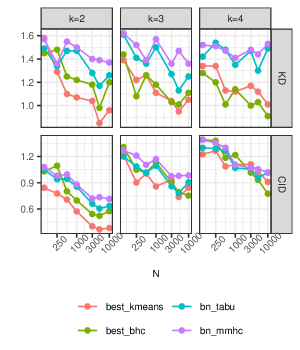
Figure 7: Results for the simulation experiments with $p=3$ binary variables.

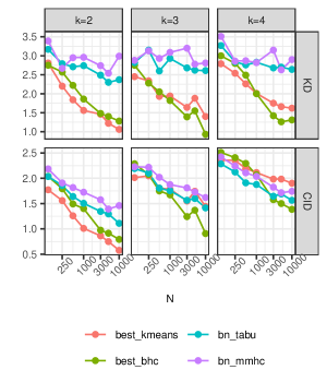
Figure 8: Results for the simulation experiments with $p=4$ binary variables.

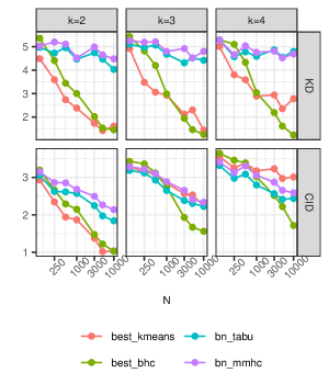
Figure 9: Results for the simulation experiments with $p=5$ binary variables.

Figure 10: Results for the simulation experiments, computational time as a function of the number of variables $p$.

D.2 Real World Examples

D.2.1 ISTAT: Aspects on Everyday Life

For the ISTAT data on aspects of everyday life we fit standard DAG categorical models using two standard state-of-the-art methods: the PC algorithm with order-invariant implementation (Colombo and Maathuis, 2014) and a hill-climbing search with tabu (Russell and Norvig, 2009) list for optimizing the BIC score, both methods are available through the bnlearn package (Scutari, 2010). In Figure 11 the CPDAGs obtained with the two methods are reported. The CPDAGs are the unique representation of the DAG Markov equivalence class. We can thus infer that both algorithms obtain a partial ordering (S,E)$\rightarrow$T, where the variable associated with watching television is estimated to be an effect of both practicing sports and the satisfaction in the environment. Similar to the results obtained with the staged tree, the PC-stable algorithm identify also a partial ordering of the variables (S,F,E)$\rightarrow$ P while the ordering among S,F, and E cannot be inferred from data. This results agree with the ones obtained through the staged tree models. The staged trees have the additional advantage of depicting context-specific conditional independences.

Figure 11: CPDAGs for the ISTAT dataset, constructed with PC-stable (left) and tabu search (right).

D.2.2 Outcomes for Hospitalised SARS-CoV-2 Patients

We report additional figures and detail on the staged tree and DAGs learned for the data on trajectories of hospitalized SARS-CoV-2 patients in France, during the first nine months of the pandemic.

Data were obtained by simulations from a probability tree where conditional probabilities were obtained from Lefrancq et al. (2021). In particular, conditional probabilities of ICU admission given age and gender and probabilities of death given ICU admission, age, and gender were obtained from the tables on the supplementary materials provided by Lefrancq et al. (2021). Marginal probabilities of gender and probabilities of age given gender were instead obtained from the linked GitHub repository.

The above conditional probabilities, define a probability event tree (a saturated staged tree model), with variables ordered gender, age, ICU, and death. Simulations can be thus performed by iterative sampling of those variables. We simulate $10000$ trajectories and we use the artificial data to learn a staged tree model using the backward hill-climbing search coupled with the dynamic programming approach for variables order.

In Figure 12 we plot the learned staged tree, we can appreciate that all nodes at depth one are in the same stage, thus the first two variables, age, and gender are inferred to be independent, their causal order is thus not discernible from data (the age distributions given gender are indeed very similar). For variables ICU and death, non-symmetrical and context-dependent conditional independences are presents.

In Figure 13 we report the CPDAG obtained with the PC-stable (Colombo and Maathuis, 2014) and tabu algorithms (Russell and Norvig, 2009). We observe that the score-based method (tabu) maximising BIC, is not able to find any ordering of the variables, except a conditional independence between gender and age. On the contrary, the PC-stable results obtain a causal order similar to the one used in the data generating mechanism and the one retrieved by the staged tree.

Figure 12: Staged tree obtained with the BHC method from the data on trajectories of covid patients.

Figure 13: CPDAGs for the covid data, constructed with PC-stable (left) and tabu search (right).

D.2.3 ENSO Effects on Spring Precipitation in Australia

We continue here the analysis of the relationship between ENSO, IOD and spring precipitation in Australia (AU). In Figure 14 we show the learned staged tree with the BHC algorithm with the alternative order IOD, ENSO, AU. The model attains an AIC of 371.04 (compared to 368.23 with the ENSO,IOD,AU order). We can observe that the staging of the AU variable is the same (obviously with a node permutation in the plots), this fact is a consequence that the optimal staging of the nodes for a given variable (AU) is not dependent on the order of the previous variables (ENSO, IOD).

Thus the only real difference between the two staged trees is in the first two variables. We can see that for the ENSO$\rightarrow$IOD order, the method recognizes a so-called partial independence between ENSO and IOD $(P(\text{IOD}|\text{ENSO}=\text{Ni\~{n}a})=P(\text{IOD}|\text{ENSO}=\text{neutral})\neq P(\text{IOD}|\text{ENSO}=\text{Ni\~{n}o})$. For the IOD$\rightarrow$ENSO model, instead no independence statement is found and the full model for the first two variables is obtained. Since the full model for ENSO and IOD could be written equivalently with either of the two variables as the first one, we can deduce that the ENSO$\rightarrow$IOD ordering is thus supported by data under the assumption that the real model is the simpler one that explains well the data.

Figure 14: Staged tree estimated with the BHC algorithm for the ENSO-IOD-AU example and estimated conditional probabilities for high AU in the three recovered stages.

References

- Barclay et al. (2013) L. M. Barclay, J. L. Hutton, and J. Q. Smith. Refining a Bayesian network using a chain event graph. International Journal of Approximate Reasoning, 54:1300–1309, 2013.
- Bhattacharya et al. (2021) R. Bhattacharya, T. Nagarajan, D. Malinsky, and I. Shpitser. Differentiable causal discovery under unmeasured confounding. In International Conference on Artificial Intelligence and Statistics, pages 2314–2322, 2021.
- Boutilier et al. (1996) C. Boutilier, N. Friedman, M. Goldszmidt, and D. Koller. Context-specific independence in Bayesian networks. In Proceedings of the 12th Conference on Uncertainty in Artificial Intelligence, pages 115–123, 1996.
- Cai et al. (2018) R. Cai, J. Qiao, K. Zhang, Z. Zhang, and Z. Hao. Causal discovery from discrete data using hidden compact representation. Advances in Neural Information Processing Systems, 2018:2666, 2018.
- Carli et al. (2022) F. Carli, M. Leonelli, E. Riccomagno, and G. Varando. The R package stagedtrees for structural learning of stratified staged trees. Journal of Statistical Software, 102(6):1–30, 2022.
- Chickering (2002) D. M. Chickering. Optimal structure identification with greedy search. Journal of Machine Learning Research, 3:507–554, 2002.
- Chickering et al. (1997) D. M. Chickering, D. Heckerman, and C. Meek. A Bayesian approach to learning Bayesian networks with local structure. In Proceedings of 13th Conference on Uncertainty in Artificial Intelligence, pages 80–89, 1997.
- Collazo and Smith (2016) R. A. Collazo and J. Q. Smith. A new family of non-local priors for chain event graph model selection. Bayesian Analysis, 11(4):1165–1201, 2016.
- Collazo et al. (2018) R. A. Collazo, C. Görgen, and J. Q. Smith. Chain event graphs. Chapmann & Hall, 2018.
- Colombo and Maathuis (2014) D. Colombo and M. H. Maathuis. Order-independent constraint-based causal structure learning. Journal of Machine Learning Research, 15(116):3921–3962, 2014.
- Cowell and Smith (2014) R. G. Cowell and J. Q. Smith. Causal discovery through MAP selection of stratified chain event graphs. Electronic Journal of Statistics, 8(1):965–997, 2014.
- Duarte and Solus (2021) E. Duarte and L. Solus. Representation of context-specific causal models with observational and interventional data. arXiv:2101.09271, 2021.
- Freeman and Smith (2011) G. Freeman and J. Q. Smith. Bayesian MAP model selection of chain event graphs. Journal of Multivariate Analysis, 102(7):1152–1165, 2011.
- Genewein et al. (2020) T. Genewein, T. McGrath, G. Déletang, V. Mikulik, M. Martic, S. Legg, and P. A. Ortega. Algorithms for causal reasoning in probability trees. arXiv:2010.12237, 2020.
- Glymour et al. (2019) C. Glymour, K. Zhang, and P. Spirtes. Review of causal discovery methods based on graphical models. Frontiers in Genetics, 10:524, 2019.
- Görgen and Smith (2018) C. Görgen and J. Q. Smith. Equivalence classes of staged trees. Bernoulli, 24(4A):2676–2692, 2018.
- Görgen et al. (2015) C. Görgen, M. Leonelli, and J. Q. Smith. A differential approach for staged trees. In European Conference on Symbolic and Quantitative Approaches to Reasoning and Uncertainty, pages 346–355, 2015.
- Görgen et al. (2018) C. Görgen, A. Bigatti, E. Riccomagno, and J. Q. Smith. Discovery of statistical equivalence classes using computer algebra. International Journal of Approximate Reasoning, 95:167–184, 2018.
- Görgen et al. (2022) C. Görgen, M. Leonelli, and O. Marigliano. The curved exponential family of a staged tree. Electronic Journal of Statistics, 16(1):2607–2620, 2022.
- Hoyer et al. (2008) P. Hoyer, D. Janzing, J. M. Mooij, J. Peters, and B. Schölkopf. Nonlinear causal discovery with additive noise models. Advances in Neural Information Processing Systems, 21:689–696, 2008.
- Huang et al. (2018) B. Huang, K. Zhang, Y. Lin, B. Schölkopf, and C. Glymour. Generalized score functions for causal discovery. In Proceedings of the 24th International Conference on Knowledge Discovery & Data Mining, pages 1551–1560, 2018.
- Irurozki et al. (2016) E. Irurozki, B. Calvo, and J. A. Lozano. PerMallows: An R package for Mallows and generalized Mallows models. Journal of Statistical Software, 71(12):1–30, 2016.
- ISTAT (2014) ISTAT. Multiscopo ISTAT – Aspetti della vita quotidiana. UniData - Bicocca Data Archive, Milano, 2014.
- Kretschmer et al. (2021) M. Kretschmer, S. V. Adams, A. Arribas, R. Prudden, N. Robinson, E. Saggioro, and T. G. Shepherd. Quantifying causal pathways of teleconnections. Bulletin of the American Meteorological Society, 102(12):"E2247–E2263, 2021.
- Lefrancq et al. (2021) N. Lefrancq, J. Paireau, N. Hozé, N. Courtejoie, Y. Yazdanpanah, L. Bouadma, P. Y. Boëlle, F. Chereau, H. Salje, and S. Cauchemez. Evolution of outcomes for patients hospitalised during the first 9 months of the SARS-CoV-2 pandemic in France: A retrospective national surveillance data analysis. The Lancet Regional Health - Europe, 5:100087, 2021.
- Leonelli (2019) M. Leonelli. Sensitivity analysis beyond linearity. International Journal of Approximate Reasoning, 113:106–118, 2019.
- Leonelli and Varando (2022a) M. Leonelli and G. Varando. Structural learning of simple staged trees. arXiv:2203.04390, 2022a.
- Leonelli and Varando (2022b) Manuele Leonelli and Gherardo Varando. Highly efficient structural learning of sparse staged trees. In Antonio Salmerón and Rafael Rumí, editors, Proceedings of The 11th International Conference on Probabilistic Graphical Models, volume 186 of Proceedings of Machine Learning Research, pages 193–204. PMLR, 05–07 Oct 2022b.
- Markham et al. (2022) A. Markham, D. Deligeorgaki, P. Misra, and L. Solus. A transformational characterization of unconditionally equivalent Bayesian Networks. In 11th International Conference on Probabilistic Graphical Models, pages 109–120, 2022.
- Monti et al. (2020) R. P. Monti, K. Zhang, and A. Hyvärinen. Causal discovery with general non-linear relationships using non-linear ICA. In Uncertainty in Artificial Intelligence, pages 186–195. PMLR, 2020.
- Pearl (2009) J. Pearl. Causality. Cambridge University Press, 2009.
- Pearl and Verma (1987) Judea Pearl and Thomas Verma. The logic of representing dependencies by directed graphs. In Proceedings of the sixth National conference on Artificial intelligence-Volume 1, pages 374–379, 1987.
- Pensar et al. (2015) J. Pensar, H. Nyman, T. Koski, and J. Corander. Labeled directed acyclic graphs: a generalization of context-specific independence in directed graphical models. Data Mining and Knowledge Discovery, 29(2):503–533, 2015.
- Pensar et al. (2016) J. Pensar, H. Nyman, J. Lintusaari, and J. Corander. The role of local partial independence in learning of Bayesian networks. International Journal of Approximate Reasoning, 69:91–105, 2016.
- Peters and Bühlmann (2015) J. Peters and P. Bühlmann. Structural intervention distance for evaluating causal graphs. Neural Computation, 27(3):771–799, 2015.
- Peters et al. (2010) J. Peters, D. Janzing, and B. Schölkopf. Identifying cause and effect on discrete data using additive noise models. In Proceedings of the 13th International Conference on Artificial Intelligence and Statistics, pages 597–604, 2010.
- Rischel and Weichwald (2021) E. F. Rischel and S. Weichwald. Compositional abstraction error and a category of causal models. In Proceedings of the 37th Conference on Uncertainty in Artificial Intelligence, pages 1013–1023, 2021.
- Russell and Norvig (2009) Stuart J Russell and Peter Norvig. Artificial intelligence: a modern approach. Elsevier, 2009. 3a Edição.
- Scutari (2010) M Scutari. Learning Bayesian networks with the bnlearn R package. Journal of Statistical Software, 35(3):1–22, 2010.
- Silander and Leong (2013) T. Silander and T. Y. Leong. A dynamic programming algorithm for learning chain event graphs. In Proceedings of the International Conference on Discovery Science, pages 201–216, 2013.
- Smith and Anderson (2008) J. Q. Smith and P. E. Anderson. Conditional independence and chain event graphs. Artificial Intelligence, 172(1):42 – 68, 2008.
- Spirtes et al. (2000) P. Spirtes, C. N. Glymour, R. Scheines, and D. Heckerman. Causation, prediction, and search. MIT Press, 2000.
- Textor et al. (2015) I. Textor, A. Idelberger, and M. Liskiewicz. Learning from pairwise marginal independencies. In Proceedings of the 31st Conference on Uncertainty in Artificial Intelligence, page 221, 2015.
- Thwaites (2013) P. Thwaites. Causal identifiability via chain event graphs. Artificial Intelligence, 195:291–315, 2013.
- Thwaites et al. (2010) P. Thwaites, J.Q. Smith, and E. Riccomagno. Causal analysis with chain event graphs. Artificial Intelligence, 174(12-13):889–909, 2010.
- Tsamardinos et al. (2006) I. Tsamardinos, L. E. Brown, and C. F. Aliferis. The max-min hill-climbing Bayesian network structure learning algorithm. Machine learning, 65(1):31–78, 2006.
- Varando et al. (2021) G. Varando, F. Carli, and M. Leonelli. Staged trees and asymmetry-labeled DAGs. arXiv:2108.01994, 2021.
- Verma and Pearl (1990) Thomas Verma and Judea Pearl. Causal networks: Semantics and expressiveness. In Ross D. Shachter, Tod S. Levitt, Laveen N. Kanal, and John F. Lemmer, editors, Uncertainty in Artificial Intelligence, volume 9 of Machine Intelligence and Pattern Recognition, pages 69–76. North-Holland, 1990.
- Wienöbst and Liskiewicz (2020) M. Wienöbst and M. Liskiewicz. Recovering causal structures from low-order conditional independencies. In Proceedings of the AAAI Conference on Artificial Intelligence, volume 34, pages 10302–10309, 2020.