CHIME/FRB Catalog 1 results: statistical cross-correlations with large-scale structure

Masoud Rafiei-Ravandi Perimeter Institute for Theoretical Physics, 31 Caroline Street N, Waterloo, ON N25 2YL, Canada Department of Physics and Astronomy, University of Waterloo, Waterloo, ON N2L 3G1, Canada Kendrick M. Smith Perimeter Institute for Theoretical Physics, 31 Caroline Street N, Waterloo, ON N25 2YL, Canada Dongzi Li Cahill Center for Astronomy and Astrophysics, California Institute of Technology, 1216 E. California Boulevard, Pasadena, CA 91125, USA Kiyoshi W. Masui MIT Kavli Institute for Astrophysics and Space Research, Massachusetts Institute of Technology, 77 Massachusetts Ave., Cambridge, MA 02139, USA Department of Physics, Massachusetts Institute of Technology, 77 Massachusetts Ave., Cambridge, MA 02139, USA Alexander Josephy Department of Physics, McGill University, 3600 rue University, Montréal, QC H3A 2T8, Canada McGill Space Institute, McGill University, 3550 rue University, Montréal, QC H3A 2A7, Canada Matt Dobbs Department of Physics, McGill University, 3600 rue University, Montréal, QC H3A 2T8, Canada McGill Space Institute, McGill University, 3550 rue University, Montréal, QC H3A 2A7, Canada Dustin Lang Perimeter Institute for Theoretical Physics, 31 Caroline Street N, Waterloo, ON N25 2YL, Canada Department of Physics and Astronomy, University of Waterloo, Waterloo, ON N2L 3G1, Canada Mohit Bhardwaj Department of Physics, McGill University, 3600 rue University, Montréal, QC H3A 2T8, Canada McGill Space Institute, McGill University, 3550 rue University, Montréal, QC H3A 2A7, Canada Chitrang Patel Department of Physics, McGill University, 3600 rue University, Montréal, QC H3A 2T8, Canada Dunlap Institute for Astronomy & Astrophysics, University of Toronto, 50 St. George Street, Toronto, ON M5S 3H4, Canada Kevin Bandura Lane Department of Computer Science and Electrical Engineering, 1220 Evansdale Drive, PO Box 6109, Morgantown, WV 26506, USA Center for Gravitational Waves and Cosmology, West Virginia University, Chestnut Ridge Research Building, Morgantown, WV 26505, USA Sabrina Berger Department of Physics, McGill University, 3600 rue University, Montréal, QC H3A 2T8, Canada McGill Space Institute, McGill University, 3550 rue University, Montréal, QC H3A 2A7, Canada P. J. Boyle Department of Physics, McGill University, 3600 rue University, Montréal, QC H3A 2T8, Canada McGill Space Institute, McGill University, 3550 rue University, Montréal, QC H3A 2A7, Canada Charanjot Brar Department of Physics, McGill University, 3600 rue University, Montréal, QC H3A 2T8, Canada Daniela Breitman Dunlap Institute for Astronomy & Astrophysics, University of Toronto, 50 St. George Street, Toronto, ON M5S 3H4, Canada Department of Physics, University of Toronto, 60 St. George Street, Toronto, ON M5S 1A7, Canada David A. Dunlap Department of Astronomy & Astrophysics, University of Toronto, 50 St. George Street, Toronto, ON M5S 3H4, Canada Tomas Cassanelli Dunlap Institute for Astronomy & Astrophysics, University of Toronto, 50 St. George Street, Toronto, ON M5S 3H4, Canada David A. Dunlap Department of Astronomy & Astrophysics, University of Toronto, 50 St. George Street, Toronto, ON M5S 3H4, Canada Pragya Chawla Department of Physics, McGill University, 3600 rue University, Montréal, QC H3A 2T8, Canada McGill Space Institute, McGill University, 3550 rue University, Montréal, QC H3A 2A7, Canada Fengqiu Adam Dong Department of Physics and Astronomy, University of British Columbia, 6224 Agricultural Road, Vancouver, BC V6T 1Z1 Canada Emmanuel Fonseca Department of Physics, McGill University, 3600 rue University, Montréal, QC H3A 2T8, Canada McGill Space Institute, McGill University, 3550 rue University, Montréal, QC H3A 2A7, Canada B. M. Gaensler Dunlap Institute for Astronomy & Astrophysics, University of Toronto, 50 St. George Street, Toronto, ON M5S 3H4, Canada David A. Dunlap Department of Astronomy & Astrophysics, University of Toronto, 50 St. George Street, Toronto, ON M5S 3H4, Canada Utkarsh Giri Perimeter Institute for Theoretical Physics, 31 Caroline Street N, Waterloo, ON N25 2YL, Canada Department of Physics and Astronomy, University of Waterloo, Waterloo, ON N2L 3G1, Canada Deborah C. Good Department of Physics and Astronomy, University of British Columbia, 6224 Agricultural Road, Vancouver, BC V6T 1Z1 Canada Mark Halpern Department of Physics and Astronomy, University of British Columbia, 6224 Agricultural Road, Vancouver, BC V6T 1Z1 Canada Jane Kaczmarek Dominion Radio Astrophysical Observatory, Herzberg Research Centre for Astronomy and Astrophysics, National Research Council Canada, PO Box 248, Penticton, BC V2A 6J9, Canada Victoria M. Kaspi Department of Physics, McGill University, 3600 rue University, Montréal, QC H3A 2T8, Canada McGill Space Institute, McGill University, 3550 rue University, Montréal, QC H3A 2A7, Canada Calvin Leung MIT Kavli Institute for Astrophysics and Space Research, Massachusetts Institute of Technology, 77 Massachusetts Ave., Cambridge, MA 02139, USA Department of Physics, Massachusetts Institute of Technology, 77 Massachusetts Ave., Cambridge, MA 02139, USA Hsiu-Hsien Lin Canadian Institute for Theoretical Astrophysics, 60 St. George Street, Toronto, ON M5S 3H8, Canada Juan Mena-Parra MIT Kavli Institute for Astrophysics and Space Research, Massachusetts Institute of Technology, 77 Massachusetts Ave., Cambridge, MA 02139, USA B. W. Meyers Department of Physics and Astronomy, University of British Columbia, 6224 Agricultural Road, Vancouver, BC V6T 1Z1 Canada D. Michilli Department of Physics, McGill University, 3600 rue University, Montréal, QC H3A 2T8, Canada McGill Space Institute, McGill University, 3550 rue University, Montréal, QC H3A 2A7, Canada Moritz Münchmeyer Department of Physics, University of Wisconsin-Madison, 1150 University Ave., Madison, WI 53706, USA Cherry Ng Dunlap Institute for Astronomy & Astrophysics, University of Toronto, 50 St. George Street, Toronto, ON M5S 3H4, Canada Emily Petroff Department of Physics, McGill University, 3600 rue University, Montréal, QC H3A 2T8, Canada McGill Space Institute, McGill University, 3550 rue University, Montréal, QC H3A 2A7, Canada Anton Pannekoek Institute for Astronomy, University of Amsterdam, Science Park 904, 1098 XH Amsterdam, The Netherlands Veni Fellow Ziggy Pleunis Department of Physics, McGill University, 3600 rue University, Montréal, QC H3A 2T8, Canada McGill Space Institute, McGill University, 3550 rue University, Montréal, QC H3A 2A7, Canada Mubdi Rahman Sidrat Research, PO Box 73527 RPO Wychwood, Toronto, ON M6C 4A7, Canada Pranav Sanghavi Lane Department of Computer Science and Electrical Engineering, 1220 Evansdale Drive, PO Box 6109, Morgantown, WV 26506, USA Center for Gravitational Waves and Cosmology, West Virginia University, Chestnut Ridge Research Building, Morgantown, WV 26505, USA Paul Scholz Dunlap Institute for Astronomy & Astrophysics, University of Toronto, 50 St. George Street, Toronto, ON M5S 3H4, Canada Kaitlyn Shin MIT Kavli Institute for Astrophysics and Space Research, Massachusetts Institute of Technology, 77 Massachusetts Ave., Cambridge, MA 02139, USA Department of Physics, Massachusetts Institute of Technology, 77 Massachusetts Ave., Cambridge, MA 02139, USA Ingrid H. Stairs Department of Physics and Astronomy, University of British Columbia, 6224 Agricultural Road, Vancouver, BC V6T 1Z1 Canada Shriharsh P. Tendulkar National Centre for Radio Astrophysics, Post Bag 3, Ganeshkhind, Pune, 411007, India Department of Astronomy and Astrophysics, Tata Institute of Fundamental Research, Mumbai, 400005, India Keith Vanderlinde Dunlap Institute for Astronomy & Astrophysics, University of Toronto, 50 St. George Street, Toronto, ON M5S 3H4, Canada David A. Dunlap Department of Astronomy & Astrophysics, University of Toronto, 50 St. George Street, Toronto, ON M5S 3H4, Canada Andrew Zwaniga Department of Physics, McGill University, 3600 rue University, Montréal, QC H3A 2T8, Canada Masoud Rafiei-Ravandi mrafieiravandi@perimeterinstitute.ca

Abstract

The CHIME/FRB Project has recently released its first catalog of fast radio bursts (FRBs), containing 492 unique sources. We present results from angular cross-correlations of CHIME/FRB sources with galaxy catalogs. We find a statistically significant ( $p\mkern 1.55mu$ -value $\sim 10^{-4}$ , accounting for look-elsewhere factors) cross-correlation between CHIME FRBs and galaxies in the redshift range $0.3\lesssim z\lesssim 0.5$ , in three photometric galaxy surveys: WISE $\times$ SCOS, DESI-BGS, and DESI-LRG. The level of cross-correlation is consistent with an order-one fraction of the CHIME FRBs being in the same dark matter halos as survey galaxies in this redshift range. We find statistical evidence for a population of FRBs with large host dispersion measure ( $\sim 400$ pc cm^-3), and show that this can plausibly arise from gas in large halos ( $M\sim 10^{14}M_{\odot}$ ), for FRBs near the halo center ( $r\lesssim 100$ kpc). These results will improve in future CHIME/FRB catalogs, with more FRBs and better angular resolution.

Radio transient sources (2008), Large-scale structure of the universe (902), High energy astrophysics (739), Cosmology (343)

1 Introduction

Fast radio bursts (FRBs) are millisecond flashes of radio waves whose dispersion is beyond what we expect from Galactic models along the line of sight. The origin of FRBs is still a mystery, despite over a decade of observations and theoretical exploration (see, e.g. Cordes & Chatterjee, 2019; Petroff et al., 2019; Platts et al., 2019). The Canadian Hydrogen Intensity Mapping Experiment / Fast Radio Burst Project (CHIME/FRB; CHIME/FRB Collaboration, 2018) has recently released its first catalog of FRBs containing 492 unique sources (CHIME/FRB Collaboration, 2021), increasing the number of known FRBs by a factor $\sim$ 4.¹¹1For a complete list of known FRBs, see https://www.herta-experiment.org/frbstats (Spanakis-Misirlis, 2021) or the Transient Name Server (TNS, Petroff & Yaron, 2020). This unprecedented sample size is a new opportunity for statistical studies of FRBs.

The angular resolution of CHIME/FRB is not sufficient to associate FRBs with unique host galaxies, except for some FRBs at very low DM, for example a repeating CHIME FRB associated with M81 (Bhardwaj et al., 2021). This appears to put some science questions out of reach, such as determining the redshift distribution of CHIME FRBs.

However, with large enough catalogs of both FRBs and galaxies, it is possible to associate FRBs with galaxies statistically, using angular cross-correlations. Intuitively, if the angular resolution $\theta_{f}$ of an FRB experiment is too large for unique host galaxy associations, there will still be an excess probability (relative to a random point on the sky) to observe FRBs within distance $\sim\theta_{f}$ of a galaxy. Formally, this corresponds to a cross-correlation between the FRB and galaxy catalogs, which we will define precisely in §3. By measuring the correlation as a function of galaxy redshift and FRB dispersion measure (DM) (defined below), the redshift distribution and related properties of the FRB population can be constrained, even in the absence of per-object associations.

FRB-galaxy cross-correlations have been proposed in a forecasting context (McQuinn, 2014; Masui & Sigurdson, 2015; Shirasaki et al., 2017; Madhavacheril et al., 2019; Rafiei-Ravandi et al., 2020; Reischke et al., 2021a; Alonso, 2021; Reischke et al., 2021b), and applied to the ASKAP and 2MPZ/HIPASS catalogs by Li et al. (2019). In this paper, we will use machinery developed by Rafiei-Ravandi et al. (2020) for modeling the FRB-galaxy cross-correlation, and disentangling it from propagation effects. This machinery uses the halo model for cosmological large-scale structure (LSS); for a review see Cooray & Sheth (2002).

Before summarizing the main results presented here, we recall the definition of FRB DM. FRBs are dispersed: the arrival time at radio frequency $\nu$ is delayed, by an amount proportional to $\nu^{-2}$ . The dispersion is proportional to the DM, defined as the free electron column density along the line of sight:

{\rm DM}\equiv\int n_{e}(x)\,dx\,.

(1)

Since FRBs have not been observed to have spectral lines, FRB redshifts are not directly observable. However, the DM is a rough proxy for redshift (Macquart et al., 2020). We write the total DM as the sum of contributions from our Galaxy and halo ( ${\rm DM}_{\rm gal}$ ), the IGM ( ${\rm DM}_{\rm IGM}$ ), and the FRB host galaxy and halo ( ${\rm DM}_{\rm host}$ ):

{\rm DM}={\rm DM}_{\rm gal}+{\rm DM}_{\rm IGM}(z)+{\rm DM}_{\rm host}\,.

(2)

The IGM contribution ${\rm DM}_{\rm IGM}(z)$ is given by the Macquart relation:

{\rm DM}_{\rm IGM}(z)=n_{e,0}\int_{0}^{z}dz^{\prime}\,f_{d}(z^{\prime})\frac{1+z^{\prime}}{H(z^{\prime})}\,,

(3)

where $f_{d}(z)$ is the mean electron ionization fraction at redshift $z$ , $n_{e,0}=2.13\times 10^{-7}\,{\rm cm}^{-3}$ is the comoving electron density, and $H(z)$ is the Hubble expansion rate. If $f_{d}$ is assumed independent of redshift, then Eq. (3) has the following useful approximation:

{\rm DM}_{\rm IGM}(z)\approx\Big{(}1000\mbox{ pc\,cm${}^{-3}$}\Big{)}f_{d}z\,.

(4)

We checked that this approximation is accurate to 6% for $z\leq 3$ , assuming that helium reionization is complete by $z=3$ . By default, we assume $f_{d}=0.9$ , which implies ${\rm DM}_{\rm IGM}(z)\approx 900z$ pc cm^-3.

We briefly summarize the main results of the paper. We find a statistically significant correlation between CHIME FRBs and galaxies in the redshift range $0.3\lesssim z\lesssim 0.5$ . The correlation is seen in three photometric galaxy surveys: WISE $\times$ SCOS, DESI-BGS, and DESI-LRG (described in §2.2). The statistical significance of the detection in each survey is $p\sim(2.7\times 10^{-5})$ , $(3.1\times 10^{-4})$ , and $(4.1\times 10^{-4})$ , respectively. These $p\mkern 1.55mu$ -values account for look-elsewhere effects, in both angular scale and redshift range. The observed level of correlation is consistent with an order-one fraction of CHIME FRBs inhabiting the same dark matter halos as galaxies in these surveys. CHIME/FRB does not resolve halos, so we cannot distinguish between FRBs in survey galaxies and FRBs in the same halos as survey galaxies.

We study the DM dependence of the FRB-galaxy correlation and find a correlation between high-DM (extragalactic ${\rm DM}\geq 785$ pc cm^-3) FRBs and galaxies at $z\sim 0.4$ . This implies the existence of an FRB subpopulation with host DM $\gtrsim 400$ pc cm^-3. Such large host DMs have not yet been seen in observations that directly associate FRBs with host galaxies. To date, 14 FRBs (excluding a Galactic magnetar, see CHIME/FRB Collaboration (2020a); Bochenek et al. (2020)) have been localized to host galaxies, all of which have ${\rm DM}_{\rm host}\lesssim 200$ pc cm^-3. In §4.2, we explain why these observations are not in conflict. We also show that host DMs $\gtrsim 400$ pc cm^-3 can arise from ionized gas in large ( $M\gtrsim 10^{14}\,M_{\odot}$ ) dark matter halos, if FRBs are located near the halo center ( $r\lesssim 100$ kpc).

This paper is structured as follows. In §2, we describe the observations and data reduction. Clustering results are presented in §3 and interpreted in §4. We conclude in §5. Throughout, we adopt a flat $\Lambda$ CDM cosmology with Hubble expansion rate $h=0.67$ , matter abundance $\Omega_{m}=0.315$ , baryon abundance $\Omega_{b}=0.048$ , initial power spectrum amplitude $A_{s}=2.10\times 10^{-9}$ , spectral index $n_{s}=0.965$ , neutrino mass $\sum_{\nu}m_{\nu}=0.06$ eV, and CMB temperature $T_{\rm CMB}=2.726$ K. These parameters are consistent with Planck results (Aghanim et al., 2020).

2 Data

2.1 FRB catalog

The first CHIME/FRB catalog is described in (CHIME/FRB Collaboration, 2021). In order to maximize localization precision and to simplify selection biases, we include only a single burst with the highest significance for each repeating FRB in this analysis. This treats repeating and nonrepeating FRBs as a single population. In future CHIME/FRB catalogs with more repeaters, it would be interesting to analyze the two populations separately. In CHIME/FRB, there is currently no evidence that repeaters and nonrepeaters have different sky distributions (CHIME/FRB Collaboration, 2021). We also exclude three sidelobe detections (FRB20190210D, FRB20190125B, FRB20190202B), leaving a sample of 489 unique sources. We do not exclude FRBs with excluded_flag=1, indicating an epoch of low sensitivity, since we expect the localization accuracy of such FRBs to be similar to the main catalog.

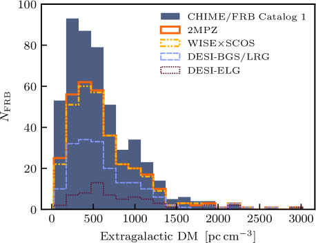
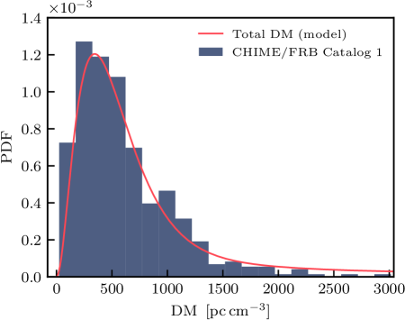
Throughout this paper, all DM values are extragalactic. That is, before further processing of the CHIME FRBs, we subtract the Galactic contribution ${\rm DM}_{\rm gal}$ from the observed DM. The value of ${\rm DM}_{\rm gal}$ is estimated using the YMW16 (Yao et al., 2017) model. In §4.2, we show that using the NE2001 (Cordes & Lazio, 2002) model does not affect results qualitatively. The CHIME/FRB extragalactic DM distribution is shown in Figure 1.

We do not subtract an estimate of the Milky Way halo DM, since the halo DM is currently poorly constrained by observations. The range of allowed values is roughly $10\lesssim{\rm DM}_{\rm halo}\lesssim 100$ pc cm^-3, and the (dipole-dominated) anisotropy is expected to be small (Prochaska & Zheng, 2019; Keating & Pen, 2020). The results of this paper are qualitatively unaffected by the value of ${\rm DM}_{\rm halo}$ .

The CHIME/FRB pipeline assigns a nominal sky location to each FRB based on the observed signal-to-noise ratio (SNR) in each of 1024 formed beams. In the simplest case of an FRB that is detected only in a single formed beam, the nominal location is the center of the formed beam. For multibeam detections, the nominal location is roughly a weighted average of the beam centers (CHIME/FRB Collaboration, 2019, 2021). Statistical errors on CHIME/FRB locations are difficult to model, since they depend on both the details of the CHIME telescope and selection biases that depend on the underlying FRB population. We discuss this further in §3.1 and Appendix A.

2.2 Galaxy catalogs

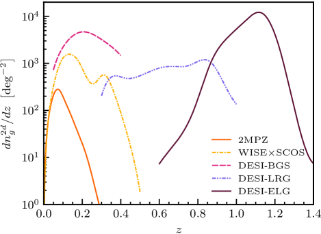
On the galaxy side, we have chosen five photometric redshift catalogs: 2MPZ, WISE $\times$ SCOS, DESI-BGS, DESI-LRG, and DESI-ELG. Note that the DESI catalogs are the photometric target samples for forthcoming spectroscopic DESI surveys with the same names. Table 1 summarizes key properties of our reduced samples for the cross-correlation analysis, and the redshift distributions are shown in Figure 1.

Survey	$f_{\rm sky}$	$[z_{\rm min},z_{\rm max}]$	$z_{\rm med}$	$N_{\rm gal}$	$N_{\rm FRB}$
2MPZ	0.647	[0.0, 0.3]	0.08	670,442	323
WISE $\times$ SCOS	0.638	[0.0, 0.5]	0.16	6,931,441	310
DESI-BGS	0.118	[0.05, 0.4]	0.22	5,304,153	183
DESI-LRG	0.118	[0.3, 1.0]	0.69	2,331,043	183
DESI-ELG	0.055	[0.6, 1.4]	1.09	5,314,194	62
BGS+LRG	0.118	[0.05, 1.0]	0.28	7,690,819	183

Table 1: Galaxy survey parameters: sky fraction

f_{\rm sky}

(not accounting for CHIME/FRB coverage), redshift range

[z_{\rm min},z_{\rm max}]

, median redshift

z_{\rm med}

, total number of unmasked galaxies

N_{\rm gal}

, and number of FRBs

N_{\rm FRB}

overlapping the survey. The “BGS+LRG” catalog is used only in §3.5, and consists of all unique objects from the DESI-BGS and DESI-LRG catalogs.

The 2MASS Photometric Redshift (2MPZ) catalog (Bilicki et al., 2013) contains $\sim$ 1 million galaxies with $z\lesssim 0.3$ (redshift error $\sigma_{z}\sim 0.02$ ), enabling the construction of a 3D view of LSS at low redshifts (see, e.g. Alonso et al., 2015; Balaguera-Antolínez et al., 2018). In this work, we use the mask made by Alonso et al. (2015) for the 2MPZ catalog. Following Bilicki et al. (2013), we discard galaxies whose $K_{s}$ -band magnitude is below the completeness limit $m_{K_{s}}=13.9$ .

The WISE $\times$ SuperCOSMOS photometric redshift catalog (WISE $\times$ SCOS, Bilicki et al., 2016) contains $\sim$ 20 million point sources with $z\lesssim 0.5$ ( $\sigma_{z}\sim 0.03$ ) over 70% of the sky, making it a versatile dataset for cross-correlation studies. In this work, we use a slightly modified catalog (Krakowski et al., 2016), which includes probabilities $(p_{\rm gal},p_{\rm star},p_{\rm qso})$ for each object to be a galaxy, star, or quasar, respectively. We use objects with $p_{\rm gal}\geq 0.9$ , which is consistent with the weighted mean purity of identified galaxies across the $W1$ band (Krakowski et al., 2016). We use a standard mask²²2http://ssa.roe.ac.uk/WISExSCOS.html to remove the Galactic foreground, Magellanic Clouds and bright stars. Additionally, we mask out regions that are contaminated visually owing to their proximity to the Galactic plane:

$\displaystyle(\|b\|\leq 20\arcdeg)$	and	$\displaystyle\left((0\arcdeg\leq l\leq 30\arcdeg)\,\mbox{or}\,(330\arcdeg\leq l\leq 360\arcdeg)\right),$
$\displaystyle(\|b\|\leq 18\arcdeg)$	and	$\displaystyle\left((30\arcdeg\leq l\leq 60\arcdeg)\,\mbox{or}\,(300\arcdeg\leq l\leq 330\arcdeg)\right),$
$\displaystyle(\|b\|\leq 17\arcdeg)$	and	$\displaystyle\left(0\arcdeg\leq l\leq 360\arcdeg\right).$	(5)

The Dark Energy Spectroscopic Instrument (DESI) Legacy Imaging Surveys (Dey et al., 2019) were designed to identify galaxies for spectroscopic follow-up. We use the catalogs from the DR8 release, with photometric redshifts from Zhou et al. (2020a). Following DESI, we consider three samples: the Bright Galaxy Survey (BGS), the Luminous Red Galaxy (LRG) sample, and the Emission Line Galaxy (ELG) sample, corresponding to redshift ranges $0.05\leq z\leq 0.4$ , $0.3\leq z\leq 1$ , and $0.6\leq z\leq 1.4$ respectively (Figure 1).

For each of the three DESI samples, we define survey geometry cuts as follows. For simplicity, we restrict to the northern part of the survey ( ${\rm Dec}>32\fdg 375$ , $b\geq+17\arcdeg$ ), which contains $\sim$ 2 times as many CHIME/FRB sources as the southern part. Note that the northern and southern DESI surveys are obtained from different telescopes and may have different systematics. For the DESI-ELG sample, we impose the additional constraint $b\geq+45\arcdeg$ in order to mitigate systematic depth variations. We restrict to sky regions that were observed at least twice in each of the $\{g,r,z\}$ bands (Zhou et al., 2020a). We mask bad pixels, bright stars, large galaxies, and globular clusters using the appropriate DESI bitmask.³³3MASKBITS 1, 5–9, and 11–13, defined here: https://www.legacysurvey.org/dr8/bitmasks/

In addition to these geometric cuts, we impose per-object cuts on the DESI catalogs by removing point-like objects (TYPE=PSF), and applying the appropriate color cuts for each of the three surveys. Color cuts for the BGS, LRG, and ELG catalogs are defined by Ruiz-Macias et al. (2020), Zhou et al. (2020b), and Raichoor et al. (2020) respectively. For BGS, we include both “faint” ( $19.5<r<20$ ) and “bright” ( $r<19.5$ ) galaxies (terminology from Ruiz-Macias et al., 2020). For BGS and LRG, we exclude objects with poorly constrained photometric redshifts ( $z_{\rm phot,std}>0.08$ ). Our final BGS, LRG and ELG samples have typical redshift error $\sigma_{z}\sim 0.03$ , 0.04, and 0.15 respectively.

Refer to caption — Figure 1: Left panel: Redshift distributions for the five galaxy samples in this paper (§2.2). Right panel: FRB extragalactic DM distributions for the CHIME/FRB catalog (solid) and for the subset of the CHIME/FRB catalog that overlaps spatially with each galaxy survey.

3 FRB-galaxy correlation results

In this section, we describe our pipeline for computing the FRB-galaxy cross power spectrum. The pipeline consists of mapping sources onto a sky grid and then computing the spherical harmonic transform and the angular power spectrum. Error bars are assigned using mock FRB catalogs.

3.1 Pipeline overview

Our central statistic is the angular power spectrum $C_{\ell}^{fg}$ , a Fourier-space statistic that measures the level of correlation between the FRB catalog $f$ and galaxy catalog $g$ , as a function of angular wavenumber $\ell$ . Formally, $C_{\ell}^{fg}$ is defined by

\big{\langle}a_{\ell m}^{f}a_{\ell^{\prime}m^{\prime}}^{g*}\big{\rangle}=C_{\ell}^{fg}\delta_{\ell\ell^{\prime}}\delta_{mm^{\prime}}\,,

(6)

where $a_{\ell m}^{Y}$ is the spherical harmonic transform of catalog $Y\in\{f,g\}$ (the all-sky analog of the Fourier transform on the flat sky). Intuitively, a detection of nonzero $C_{\ell}^{fg}$ at wavenumber $\ell$ corresponds to a pixel-space angular correlation at separation $\theta\sim\ell^{-1}$ .

The power spectrum $C_{\ell}^{fg}$ is not the only way of representing a cross-correlation between catalogs as a function of scale. Another possibility is the correlation function $\zeta(\theta)$ , obtained by counting pairs of objects whose angular separation $\theta$ lies in a set of nonoverlapping bins. This method was used by Li et al. (2019) to correlate ASKAP FRBs with nearby galaxies. The power spectrum $C_{\ell}^{fg}$ and correlation function $\zeta(\theta)$ are related to each other by the Legendre transform $\zeta(\theta)=\sum_{\ell}(2\ell+1)/(4\pi)C_{\ell}^{fg}P_{\ell}(\cos\theta)$ . Therefore, $C_{\ell}^{fg}$ and $\zeta(\theta)$ contain the same information, and the choice of which one to use is a matter of convenience. We have used the power spectrum $C_{\ell}^{fg}$ , since it has the property that nonoverlapping $\ell$ -bins are nearly uncorrelated, making it straightforward to infer statistical significance from plots.

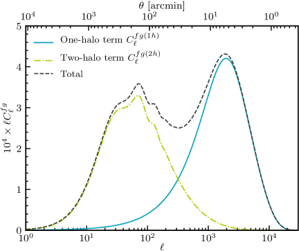
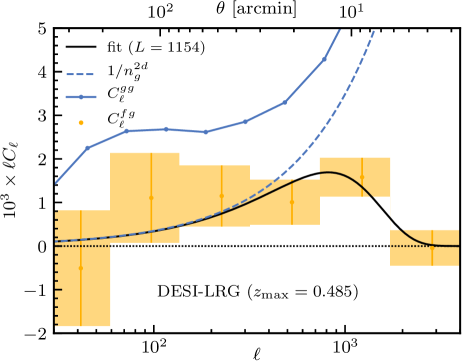
Throughout the paper, it will be useful to have a model FRB-galaxy power spectrum $C_{\ell}^{fg}$ in mind. In Figure 2, we show $C_{\ell}^{fg}$ for a galaxy population at $z\sim 0.4$ , calculated using the “high- $z$ ” FRB model from Rafiei-Ravandi et al. (2020), with median FRB redshift $z=0.76$ . The main features of $C_{\ell}^{fg}$ are as follows:

•

The leftmost peak at $\ell\sim 10^{2}$ is the two-halo term $C_{\ell}^{fg(2h)}$ , which arises from FRBs and galaxies in different halos. The two-halo term does not probe the details of FRB-galaxy associations; it arises because FRBs and galaxies both inhabit halos, and halos are clustered on $\sim 100$ Mpc scales (the correlation length of the cosmological density field).
•

The rightmost peak at $\ell\sim 10^{3}$ is the one-halo term $C_{\ell}^{fg(1h)}$ , which is sourced by (FRB, galaxy) pairs in the same dark matter halo.
•

For completeness, we note that for $\ell\gtrsim 10^{4}$ , there is a “Poisson” term (not shown in Figure 2) that is sourced by FRBs in catalog galaxies (not elsewhere in the halo). CHIME/FRB’s limited angular resolution suppresses $C_{\ell}^{fg}$ at high $\ell$ , hiding the Poisson term. Intuitively, this is because CHIME/FRB cannot resolve different galaxies in the same dark matter halo.

Although the one-halo and two-halo terms look comparable in Figure 2, the SNR of the one-halo term is a few times larger. In this paper, we do not detect the two-halo term with statistical significance (see Figure 7). Therefore, throughout the paper we will often neglect the two-halo term, and make the approximation $C_{\ell}^{fg}\approx C_{\ell}^{fg(1h)}$ .

The one-halo term $C_{\ell}^{fg(1h)}$ is constant in $\ell$ for $\ell\lesssim 10^{3}$ , and suppressed for $\ell\gtrsim 10^{3}$ . (Note that in Figure 2, we have plotted $\ell C_{\ell}^{fg}$ , for consistency with later figures in the paper.) The high- $\ell$ suppression arises from two effects: (1) statistical errors on FRB positions (the CHIME/FRB “beam”), and (2) displacements between FRBs and galaxies in the same dark matter halo.

Within the statistical errors of the $C_{\ell}^{fg}$ measurement in this paper, both effects can be modeled as Gaussian, i.e. high- $\ell$ suppression of the form $e^{-\ell^{2}/L^{2}}$ :

C_{\ell}^{fg(1h)}=\alpha e^{-\ell^{2}/L^{2}}\,,

(7)

where we have omitted the two-halo term since we do not detect it with statistical significance. In principle, the value of $L$ in Eq. (7) is computable, given models for statistical errors on CHIME FRB sky locations and FRB/galaxy profiles within dark matter halos. However, FRB halo profiles are currently poorly constrained, and CHIME FRB location errors are difficult to model, since they depend on both instrumental selection effects and details of the FRB population. In Appendix A, we explore modeling issues in detail and show that a plausible (but conservative, i.e. wide) range of $L$ -values is $315\leq L\leq 1396$ .

Summarizing the above discussion, our pipeline works as follows. We measure the angular power spectrum $C_{\ell}^{fg}$ from the FRB and galaxy catalogs, and fit the $\ell$ -dependence to the template form $C_{\ell}^{fg}=\alpha e^{-\ell^{2}/L^{2}}$ in Eq. (7). We treat the amplitude $\alpha$ as a free parameter, and vary the template scale $L$ over the range $315\leq L\leq 1396$ , to evaluate the correlation amplitude as a function of scale.

3.2 Overdensity maps

Turning now to implementation, the first step in our pipeline is to convert the FRB and galaxy catalogs into “overdensity” maps $\delta_{f}({\bf x}),\delta_{g}({\bf x})$ , defined by

\delta_{Y}({\bf x})=\frac{1}{n_{Y}^{2d}\,\Omega_{\rm pix}}\Big{(}N_{Y\in{\bf x}}-\overline{N_{Y\in{\bf x}}}\Big{)}\,.

(8)

Here, $Y\in\{f,g\}$ denotes a catalog, ${\bf x}$ denotes an angular pixel, $N_{Y\in{\bf x}}$ denotes the number of catalog objects in pixel ${\bf x}$ , and $\overline{N_{Y\in{\bf x}}}$ denotes the expected number of catalog objects in pixel ${\bf x}$ due to the survey geometry. The prefactor $1/(n_{Y}^{2d}\Omega_{\rm pix})$ is conventional, where $n_{Y}^{2d}$ is the 2D number density and $\Omega_{\rm pix}$ is the pixel area. For CHIME/FRB, the expected number density $\smash{\overline{N}_{f\in{\bf x}}}$ depends on declination (Dec). The definition (8) of $\delta_{f}({\bf x})$ weights each pixel ${\bf x}$ proportionally to the expected number of FRBs. This weighting is optimal since the FRB field is Poisson noise dominated $(C_{\ell}^{ff}\approx 1/n_{f}^{2d})$ .

The difference between a density map and an overdensity map is the second term $\bar{N}$ in Eq. (8), which removes spurious density fluctuations due to the survey geometry. We compute the $\bar{N}$ -term differently for different catalogs as follows.

For the three DESI catalogs, we estimate $\bar{N}$ using “randoms” from the DESI-DR8 release, i.e. simulated catalogs that encode the survey geometry, with no spatial correlations between objects. We use random catalogs from the DESI-DR8 data release (source density $n_{g}^{2d}=5000$ deg^-2), and apply the DESI “geometry” cuts from the previous section.

For the other two galaxy surveys (2MPZ and WISE $\times$ SCOS), random catalogs are not readily available, so we represent the survey geometry by an angular HEALPix (Gorski et al., 2005) mask, and assume uniform galaxy density outside the mask:

\bar{N}_{g\in{\bf x}}=\left\{\begin{array}[]{cl}n_{g}^{2d}\,\Omega_{\rm pix}&\mbox{if ${\bf x}$ is unmasked}\\ 0&\mbox{if ${\bf x}$ is masked}\end{array}\right.

(9)

The mask geometries for 2MPZ and WISE $\times$ SCOS were described previously in §2.2.

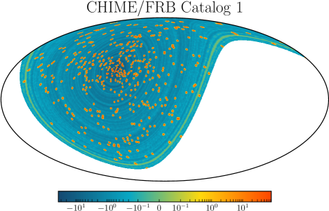
Finally, for the CHIME/FRB catalog, computing $\bar{N}$ deserves some discussion. The CHIME/FRB number density $\bar{N}$ is inhomogeneous, peaking near the north celestial pole. To an excellent approximation, the number density is azimuthally symmetric in equatorial coordinates, i.e. independent of right ascension (RA) at fixed declination, because CHIME is a cylindrical drift-scan telescope oriented north-south (CHIME/FRB Collaboration, 2021). Therefore, we make random FRB catalogs that represent $\bar{N}$ by randomizing RAs of the FRBs in the observed catalog, leaving declinations fixed. When making randoms, we also loop over 1000 copies of the CHIME/FRB catalog, so that the random catalogs are much larger than the data catalog (appropriately rescaling $\bar{N}$ and $n_{f}^{2d}$ in Eq. 8).

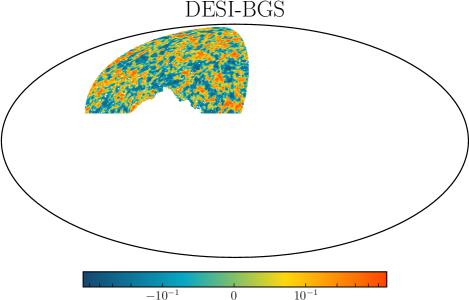
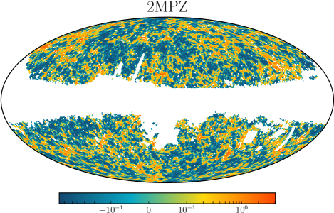
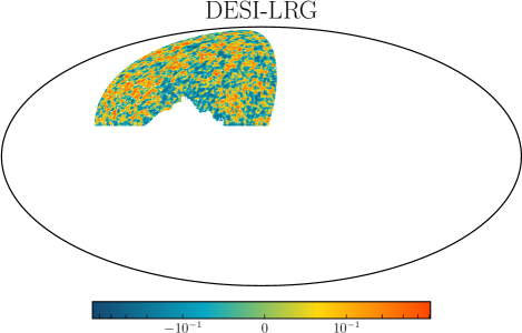
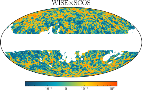
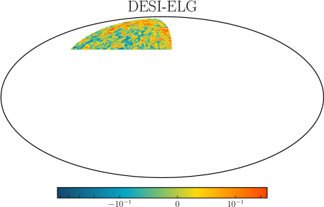
In Figure 3, we show overdensity maps $\delta_{Y}({\bf x})$ for the CHIME/FRB sources and the galaxies. These maps are useful as visual checks for systematic effects, before catalogs are cross-correlated. For example, if the Galactic mask is not conservative enough, the overdensity map may show visual artifacts with $\delta_{g}<0$ , since Galactic extinction will suppress the observed catalog density $N$ , relative to $\bar{N}$ . No visual red flags are seen in either the CHIME/FRB or galaxy maps, even without a Galactic mask for CHIME/FRB. This is consistent with Josephy et al. (2021), who found no evidence for Galactic latitude dependence in the CHIME/FRB number density after correcting for selection effects. As described in §2.2, we do apply a Galactic mask in our pipeline, so even if the FRB catalog does contain low-level biases in the Galactic plane, they should be mitigated.

3.3 Estimating the power spectrum $C_{\ell}^{fg}$

We estimate $C_{\ell}^{fg}$ in our pipeline by taking spherical transforms of the overdensity maps $\delta_{f}({\bf x}),\delta_{g}({\bf x})$ , to get spherical harmonic coefficients $a_{\ell m}^{f}$ and $a_{\ell m}^{g}$ . Then, we estimate the power spectrum $C_{\ell}^{fg}$ as

{\hat{C}}_{\ell}^{fg}=\frac{1}{f_{\rm sky}^{fg}}\sum_{m=-\ell}^{\ell}\frac{1}{2\ell+1}a_{\ell m}^{f*}a_{\ell m}^{g}\,,

(10)

where $f_{\rm sky}^{fg}$ is the fractional sky area subtended by the intersection of the FRB and galaxy surveys. The $f_{\rm sky}^{fg}$ prefactor normalizes the power spectrum estimator to have the correct normalization on the partial sky. Throughout the main analysis, we represent overdensities as HEALPix maps with $1\farcm 7$ resolution ( $N_{\rm side}=2048$ ), and estimate the power spectrum to a maximum multipole of $\ell_{\rm max}=2000$ , corresponding to angular scale $\theta=\pi/\ell_{\rm max}=5\farcm 4$ .

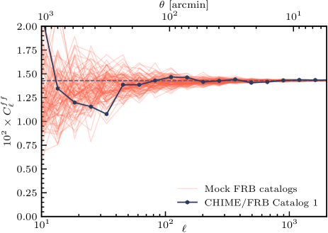
We assign error bars to the power spectrum $C_{\ell}^{fg}$ using Monte Carlo techniques, simulating mock FRB catalogs and cross-correlating them with the real galaxy catalogs. We simulate mock FRB catalogs by keeping FRB declinations the same as in the real catalog, but randomizing right ascensions. This mimics the logic used to construct random FRB catalogs in §3.2. In fact, the only difference in our pipeline between a “mock” and a “random” FRB catalog is the number of FRBs: a mock catalog has the same number of FRBs as the data, whereas a random catalog has a much larger number. Conceptually, there is another difference between mocks and randoms: mocks should include any spatial clustering signal present in the real data, whereas randoms are unclustered and only represent the survey geometry. For FRBs, spatial clustering is small compared to Poisson noise ( $C_{\ell}^{ff}$ $\approx 1/n_{f}^{2d}$ , see Figure 5), so we can make the approximation that clustering is negligible.

3.4 Statistical significance and look-elsewhere effect

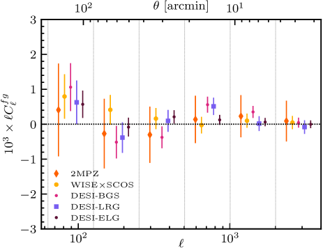
In Figure 4, we show the angular power spectrum $C_{\ell}^{fg}$ for a set of nonoverlapping $\ell$ bins. A weak positive FRB-galaxy correlation is seen at $500\lesssim\ell\lesssim 1000$ in some of the galaxy surveys. In this subsection, we will address the question of whether this correlation is statistically significant.

As explained in §3.1, we will fit the FRB-galaxy correlation to the template $C_{\ell}^{fg}=\alpha e^{-\ell^{2}/L^{2}}$ , treating the amplitude $\alpha$ as a free parameter, and varying the template scale $L$ over the range $315\leq L\leq 1396$ . Let us temporarily assume that $L$ is known in advance. In this case, an optimal estimator for $\alpha$ is

\hat{\alpha}_{L}=\frac{1}{{\mathcal{N}}_{L}}\sum_{\ell\geq\ell_{\rm min}}(2\ell+1)\frac{e^{-\ell^{2}/L^{2}}}{C_{\ell}^{gg}}{\hat{C}}_{\ell}^{fg}\,,

(11)

where ${\hat{C}}_{\ell}^{fg}$ was defined in Eq. (10), and the normalization ${\mathcal{N}}_{L}$ is defined by

{\mathcal{N}}_{L}=\sum_{\ell\geq\ell_{\rm min}}(2\ell+1)\frac{e^{-2\ell^{2}/L^{2}}}{C_{\ell}^{gg}}\,.

(12)

We have included a cutoff at $\ell_{\rm min}=50$ to mitigate possible large-scale systematics. This is a conservative choice, since Figure 5 does not show evidence for systematic power in the auto power spectrum $C_{\ell}^{ff}$ for $\ell\gtrsim 15$ . Eq. (11) is derived by noting that

	$\displaystyle\mbox{Var}({\hat{C}}_{\ell}^{fg})$	$\displaystyle\propto\frac{C_{\ell}^{ff}C_{\ell}^{gg}+(C_{\ell}^{fg})^{2}}{2\ell+1}$
		$\displaystyle\propto\frac{C_{\ell}^{gg}}{2\ell+1}\,,$		(13)

where the first line follows from Wick’s theorem, and the second line follows since $(C_{\ell}^{fg})^{2}\ll C_{\ell}^{ff}C_{\ell}^{gg}$ , and $C_{\ell}^{ff}$ is nearly constant in $\ell$ .

We define the quantity

{\rm SNR}_{L}=\frac{\hat{\alpha}_{L}}{\mbox{Var}(\hat{\alpha}_{L})^{1/2}}\,,

(14)

which is the statistical significance of the $C_{\ell}^{fg}$ detection in “sigmas”, for a fixed choice of $L$ . In Figure 6, we show the quantity ${\rm SNR}_{L}$ , as a function of scale $L$ .

We pause for a notational comment: throughout the paper, $\ell$ denotes a multipole (as in $C_{\ell}^{fg}$ ), and $L$ denotes the template scale defined in Eq (7). The value of ${\rm SNR}_{L}$ (or $\hat{\alpha}_{L}$ ) is obtained by summing $C_{\ell}^{fg}$ over $\ell\lesssim L$ , as in Eq. (11). When $C_{\ell}^{fg}$ is computed as a function of $\ell$ (Figure 4), neighboring $\ell$ bins are nearly uncorrelated, whereas when ${\rm SNR}_{L}$ is computed as a function of $L$ (Figure 6), nearby $L$ -values are highly correlated.

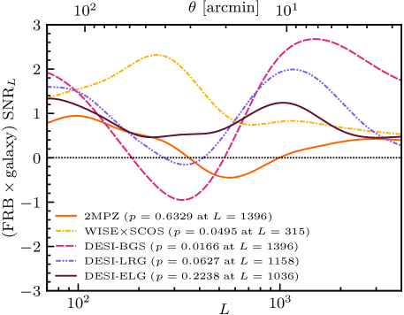
In Figure 6, it is seen that ${\rm SNR}_{L}$ can be as large as 2.67, for a certain choice of $L$ and galaxy survey (namely DESI-BGS at $L=1396$ ). However, it would be incorrect to interpret this as a 2.67 $\sigma$ detection, since the value of $L$ has been cherry-picked to maximize the signal.

To quantify statistical significance in a way that accounts for the choice of $L$ (the “look-elsewhere effect”), we restrict the search to $315\leq L\leq 1396$ and define

{\rm SNR}_{\rm max}=\max_{315\leq L\leq 1396}{\rm SNR}_{L}\,.

(15)

For fixed $L$ , ${\rm SNR}_{L}$ is approximately Gaussian distributed, and represents statistical significance in “sigmas”. Since ${\rm SNR}_{\rm max}$ is obtained by maximizing over trial $L$ -values, ${\rm SNR}_{\rm max}$ is non-Gaussian, and we assign statistical significance by Monte Carlo inference.

In more detail, we compare the “data” value of ${\rm SNR}_{\rm max}$ (e.g. ${\rm SNR}_{\rm max}=2.67$ for DESI-BGS) to an ensemble of Monte Carlo simulations, obtained by cross-correlating mock FRB catalogs with the real galaxy catalog as in §3.3. We assign a $p\mkern 1.55mu$ -value by computing the fraction of mocks with ${\rm SNR}_{\rm max}^{\rm(mock)}\geq{\rm SNR}_{\rm max}^{\rm(data)}$ . We find $p=0.0166$ for DESI-BGS, i.e. evidence for a correlation at 98.34% CL after accounting for the look-elsewhere effect in $L$ . The $p\mkern 1.55mu$ -values for the other galaxy surveys are shown in Figure 6.

Our interpretation is that this level of evidence is intriguing, but not high enough to be conclusive. Therefore, we do not interpret the FRB-galaxy correlation in Figures 4 and 6 as a detection. However, in the next subsection we will restrict the redshift range of the galaxy catalog (accounting for the look-elsewhere effect in choice of redshift range) and find a high-significance detection.

3.5 Redshift dependence

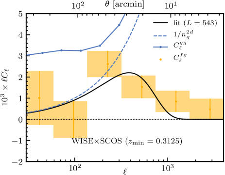
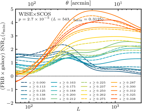
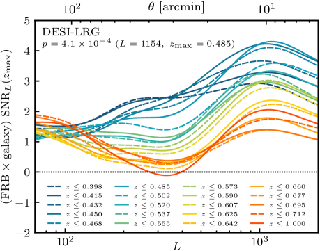
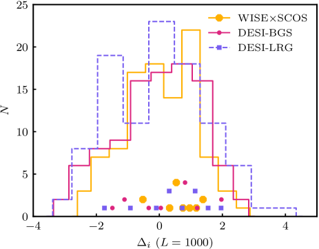
To illustrate our method for studying redshift dependence, we will use the WISE $\times$ SCOS galaxy catalog as a running example. Suppose we cross-correlate CHIME FRBs with WISE $\times$ SCOS galaxies above some minimum redshift $z_{\rm min}$ , where $z_{\rm min}$ is a free parameter that will be varied. For each $z_{\rm min}$ , we repeat the analysis of the previous subsection. The power spectrum $C_{\ell}^{fg}(z_{\rm min})$ and quantity ${\rm SNR}_{L}(z_{\rm min})$ (defined in Eq. 14) are now functions of two parameters: $z_{\rm min}$ and template scale $L$ .

In the top panels of Figure 7, we show the power spectrum $C_{\ell}^{fg}(z_{\rm min})$ for the fixed choice of redshift $z_{\rm min}=0.3125$ , and ${\rm SNR}_{L}(z_{\rm min})$ as a function of $L$ and $z_{\rm min}$ . For specific parameter choices, we see a large FRB-galaxy correlation, e.g. ${\rm SNR}_{L}(z_{\rm min})=4.88$ at $L=543$ and $z_{\rm min}=0.3125$ . As in the previous subsection, this would imply a 4.88 $\sigma$ cross-correlation for these cherry-picked values of $(L,z_{\rm min})$ , but does not account for the look-elsewhere effect in choosing these values.

To assign statistical significance in a way that accounts for the look-elsewhere effect, we use the same method as the previous subsection, except that we now scan over two parameters $(L,z_{\rm min})$ rather than one $(L)$ . Formally, we define

{\rm SNR}_{\rm max}=\max_{0\leq z_{\rm min}\leq 0.5}\,\,\max_{315\leq L\leq 1396}{\rm SNR}_{L}(z_{\rm min})\,,

(16)

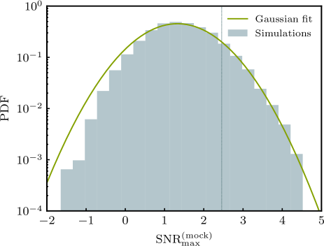
analogously to Eq. (15) from the previous subsection. To assign bottom-line statistical significance, we would like to rank the “data” value ${\rm SNR}_{\rm max}=4.88$ within a histogram of ${\rm SNR}_{\rm max}$ values obtained by cross-correlating mock FRB catalogs with the galaxy catalog. However, with $10^{4}$ simulations, we find that none of the mock catalogs actually exceed ${\rm SNR}_{\rm max}=4.88$ , so we fit the tail of the ${\rm SNR}_{\rm max}$ distribution to an analytic distribution (a truncated Gaussian), and compute the $p\mkern 1.55mu$ -value analytically. For details of the tail-fitting procedure, see Appendix C. We obtain detection significance $p=2.7\times 10^{-5}$ for WISE $\times$ SCOS with $z_{\rm min}=0.3125$ . This analysis “scans” over minimum redshift $z_{\rm min}$ and scale $L$ , and the significance fully accounts for the look-elsewhere effect in these parameters.

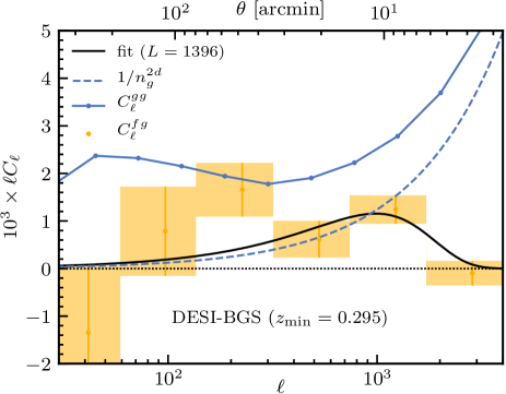
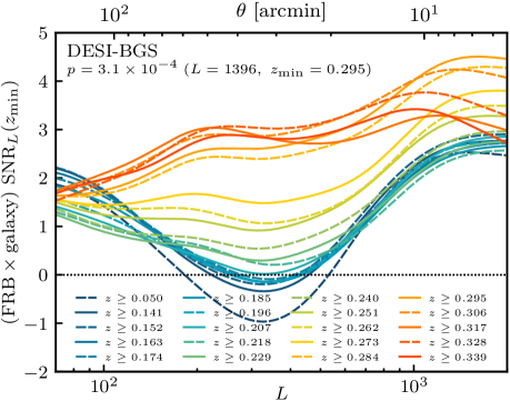
Similarly, we get $p=3.1\times 10^{-4}$ for DESI-BGS with $z_{\rm min}=0.295$ , scanning over $z_{\rm min}$ and $L$ . For DESI-LRG, we use a maximum redshift $z_{\rm max}$ instead of a minimum redshift $z_{\rm min}$ , since DESI-LRG is at higher redshift than WISE $\times$ SCOS or DESI-BGS (Figure 1). Scanning over $z_{\rm max}$ and scale $L$ , we obtain $p=4.1\times 10^{-4}$ with $z_{\rm max}=0.485$ for DESI-LRG. These results are shown in Figure 7.

Finally, we find borderline evidence $p=0.0421~{}(L=1396,z_{\rm max}=0.86)$ for a cross-correlation between DESI-ELG galaxies (varying $z_{\rm max}$ ) and CHIME FRBs with ${\rm DM}\geq 500$ pc cm^-3, where the choice of minimum DM is fixed. To justify this choice of ${\rm DM}_{\rm min}$ , note that since host DMs must be positive, we do not expect a correlation between DESI-ELG galaxies ( $z_{\rm min}=0.6$ ) and CHIME FRBs with ${\rm DM}<500$ pc cm^-3 (allowing for statistical fluctuations in ${\rm DM}_{\rm IGM}$ on the order of 40 pc cm^-3). We do not find any statistically significant detection with 2MPZ.

These results are consistent with a simple picture in which the FRB-galaxy correlation mainly comes from galaxies in redshift range $0.3\lesssim z\lesssim 0.5$ . For WISE $\times$ SCOS and DESI-BGS, the maximum survey redshifts are 0.5 and 0.4 respectively, and we find a strong detection when we impose a minimum redshift $z_{\rm min}\sim 0.3$ . For DESI-LRG, the minimum survey redshift is 0.3, and we find a strong detection when we impose a maximum redshift $z_{\rm max}\sim 0.5$ . The borderline detection in DESI-ELG and nondetection in 2MPZ are also consistent with this picture, in the sense that these catalogs do not overlap with the redshift range $0.3\lesssim z\lesssim 0.5$ .

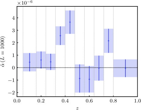
As a direct way of seeing that the FRB-galaxy correlation is sourced by redshift range $0.3\lesssim z\lesssim 0.5$ , in Figure 8 we cross-correlate the FRB catalog with the combined BGS+LRG catalog (Table 1, bottom row) in nonoverlapping redshift bins with $0.05\leq z\leq 1$ . It is seen that the cross-correlation is driven by redshift range $0.3\lesssim z\lesssim 0.5$ . (The bin at $z\sim 0.75$ is nonzero at 2.2 $\sigma$ , which we interpret as borderline statistical significance, since there are 10 bins.)

In Appendix B, we examine the robustness of these results using null tests and do not find any evidence for systematic biases.

4 Interpretation

So far, we have concentrated on establishing statistical significance of the FRB-galaxy correlation, in a Monte Carlo simulation pipeline that accounts for look-elsewhere effects. In this section, we will interpret the FRB-galaxy correlation, and explore implications for FRBs.

As explained in §3.1, the output of our pipeline is a constraint on the coefficient $\alpha$ in the template fit:

C_{\ell}^{fg}\approx C_{\ell}^{fg(1h)}\approx\alpha e^{-\ell^{2}/L^{2}}\,,

(17)

where the factor $e^{-\ell^{2}/L^{2}}$ is a Gaussian approximation to the high- $\ell$ suppression due to FRB/galaxy profiles and the instrumental beam.

At several points in this section, we will want to compare our FRB-galaxy correlation results to a model for $C_{\ell}^{fg(1h)}$ . To do this, we intepret the low- $\ell$ limit of the model as a prediction for the coefficient $\alpha$ above. Formally, we define

\alpha\equiv\lim_{\ell\rightarrow 0}C_{\ell}^{fg(1h)}

(18)

and compare this model prediction for $\alpha$ to the value of $(\hat{\alpha}_{L})_{L=1000}$ , where the estimator $\hat{\alpha}_{L}$ was defined in Eq. (11). For simplicity we will fix $L=1000$ , since this gives a high-significance detection of the FRB-galaxy correlation in all three galaxy surveys (see Figure 7).

4.1 Link counting

In this subsection, we will interpret the amplitude of the FRB-galaxy correlation $C_{\ell}^{fg}$ in an intuitive way. First, we fix a galaxy catalog and redshift range. As a definition, we say that an FRB is linked to a galaxy if they are in the same dark matter halo. For each FRB $f$ , we define the link count $\eta_{f}$ by

\eta_{f}=\mbox{number of survey galaxies linked to FRB $f$.}

(19)

Given an FRB catalog, we define the mean link count $\eta$ :

\eta=\big{\langle}\eta_{f}\big{\rangle}\,,

(20)

where the expectation value $\langle\cdot\rangle$ is taken over FRBs in the catalog.

To connect these definitions with our FRB-galaxy correlation results, we note that:

\alpha=\lim_{\ell\rightarrow 0}C_{\ell}^{fg(1h)}=\frac{\eta}{n_{g}^{2d}}\,,

(21)

where the first equality is Eq. (18), and the second equality follows from a short halo model calculation (Rafiei-Ravandi et al., 2020). That is, the amplitude $\alpha$ of the FRB-galaxy correlation (in the one-halo regime) is equivalent to a measurement of the mean link count $\eta$ . This provides a more intuitive interpretation of the amplitude.

In each row of Table 2, we specify a choice of galaxy catalog and redshift range. The redshift ranges have been chosen to maximize $C_{\ell}^{fg}$ , as in §3.4. In the third column, we give the constraint on $\alpha$ obtained from the estimator $\hat{\alpha}_{L}$ at $L=1000$ . In the last column, we have translated this constraint of $\alpha$ to a constraint on $\eta$ , using Eq. (21).

Taken together, the $\eta$ measurements in Table 2 show that the CHIME/FRB catalog has mean link counts of order unity with galaxies in the range $0.3\lesssim z\lesssim 0.5$ . The precise value of $\eta$ depends on the specific galaxy survey considered. Note that different galaxy surveys will have different values of $\eta$ , since the number of galaxies per halo (and to some extent the population of halos that is sampled) will be different.

Since FRBs outside the redshift range of the galaxy catalog do not contribute to $\eta$ , we write $\eta=p\tilde{\eta}$ , where $p$ is the probability that an FRB is in the catalog redshift range and $\tilde{\eta}$ is the mean link count of FRBs that are in the catalog redshift range.

For the galaxy surveys considered here, we expect $\tilde{\eta}$ to be of order unity, since dark matter halos rarely contain more than a few catalog galaxies. To justify this statement, we note that $C_{\ell}^{gg}$ is $\sim 2$ times larger than the Poisson noise $1/n_{g}^{2d}$ in the one-halo regime (see Figure 7). By a link counting argument similar to Eq. (21), this implies that $\langle N_{g}^{2}\rangle\sim 2\langle N_{g}\rangle$ , where $N_{g}$ is the number of galaxies in a halo, and the expectation values are taken over halos.

Since $\eta=p\tilde{\eta}$ is of order unity (by Table 2), and $\tilde{\eta}$ is of order unity (by the argument in the previous paragraph), we conclude that $p$ is of order unity. That is, an order-one fraction of CHIME FRBs are in the redshift range $0.3\lesssim z\lesssim 0.5$ .

We have phrased this conclusion as a qualitative statement (“order-one fraction”) since it is difficult to assign a precise upper bound to $\tilde{\eta}$ . More generally, it is difficult to infer the FRB redshift distribution $(dn_{f}^{2d}/dz)$ from the FRB-galaxy correlation in the one-halo regime, since the level of correlation is proportional to $\tilde{\eta}(dn_{f}^{2d}/dz)$ , with no obvious way of disentangling the two factors. Future CHIME/FRB catalogs should contain enough FRBs to detect the FRB-galaxy correlation on two-halo scales ( $\ell\sim 100$ ) (Rafiei-Ravandi et al., 2020), which will help break the degeneracy and measure $(dn_{f}^{2d}/dz)$ and $\tilde{\eta}$ separately.

Survey	$[z_{\rm min},z_{\rm max}]$	$(\alpha_{L})_{L=1000}$	$n_{g}^{2d}$ [sr^-1]	$\eta$
WISE $\times$ SCOS	[0.3125, 0.5]	$(4.35\pm 0.97)\times 10^{-6}$	$9.92\times 10^{4}$	$0.432\pm 0.096$
DESI-BGS	[0.295, 0.4]	$(2.69\pm 0.67)\times 10^{-6}$	$7.94\times 10^{5}$	$2.13\pm 0.53$
DESI-LRG	[0.3, 0.485]	$(3.94\pm 0.93)\times 10^{-6}$	$2.83\times 10^{5}$	$1.11\pm 0.26$

Table 2: Clustering analysis in §4.1. The FRB-galaxy clustering statistic

\alpha_{L}

(Eq. 11) can be translated to a constraint on

\eta

, the average number of survey galaxies in the same dark matter halo as a CHIME/FRB source (see text for details). The statistical error on

\eta

in each row is roughly proportional to

n_{g}^{2d}

4.2 DM dependence

In Figure 9, we divide the FRB catalog into extragalactic DM bins and explore the DM dependence of the FRB-galaxy cross-correlation.

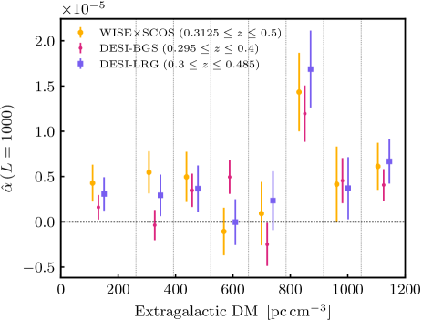
A striking feature in Figure 9 is the nonzero correlation in the three highest-DM bins, corresponding to extragalactic DM $\geq 785$ pc cm^-3.⁴⁴4A technical comment here: for some DM bins in Figure 9, the large values of $C_{\ell}^{fg}$ lead to link counts $\eta$ that are a few times larger than the link counts reported in Table 2 for the whole catalog, although statistical errors are large. However, the correlation coefficient between the FRB and galaxy fields is never larger than 1. In all cases, the field-level correlation $C_{\ell}^{fg}/(C_{\ell}^{ff}C_{\ell}^{gg})^{1/2}$ is of order 0.01 or smaller. For reference, the last three bins represent 7%, 6%, and 15% of the CHIME/FRB catalog, respectively. At the redshift of the galaxy surveys ( $z\sim 0.4$ ), the IGM contribution to the DM is ${\rm DM}_{\rm IGM}(z)\sim 360$ pc cm^-3. Therefore, the observed FRB-galaxy correlation at ${\rm DM}\geq 785$ pc cm^-3 is evidence for a subpopulation of FRBs with host DMs of order ${\rm DM}_{\rm host}\sim 400$ pc cm^-3.

This may appear to be in tension with recent direct associations between FRBs and host galaxies, which have typically been studied only for lower-redshift FRBs. At the time of this writing, 14 FRBs have been localized to host galaxies,⁵⁵5https://frbhosts.org/#explore all of which have ${\rm DM}_{\rm host}\lesssim 200$ pc cm^-3 (Spitler et al., 2016; Bassa et al., 2017; Chatterjee et al., 2017; Kokubo et al., 2017; Tendulkar et al., 2017; Bannister et al., 2019; Prochaska et al., 2019; Ravi et al., 2019; Chittidi et al., 2020; Heintz et al., 2020; Law et al., 2020; Macquart et al., 2020; Mannings et al., 2021; Marcote et al., 2020; Simha et al., 2020; Bhandari et al., 2020a, b; CHIME/FRB Collaboration, 2020b; Bhardwaj et al., 2021; James et al., 2021a). The rest of this section is devoted to interpreting this result further.

In Figure 9, the DM bin at $785<{\rm DM}<916$ pc cm^-3 is an outlier, suggesting a narrow feature in the DM dependence of the FRB-galaxy correlation. Given the error bars, it is difficult to say with statistical significance whether the apparent narrowness is real, or whether the true DM dependence is slowly varying. A crucial point here is that the three galaxy catalogs are highly correlated spatially (after restricting to the appropriate redshift ranges), which implies that the three measurements in Figure 9 have highly correlated statistical errors. Future CHIME/FRB catalogs will have smaller error bars and can statistically distinguish a narrow feature from slowly varying DM dependence.

As a check, we remade Figure 9 using the NE2001 (Cordes & Lazio, 2002) model for Galactic DM, instead of the YMW16 model. The effect of this change is small compared to the statistical errors in Figure 9.

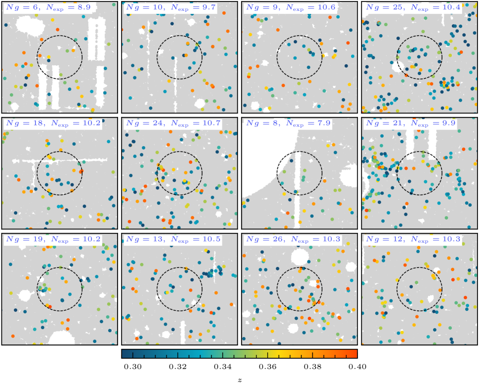
We also performed the following visual check. The outlier bin with $785<{\rm DM}<916$ pc cm^-3 in Figure 9 only contains 12 FRBs in the DESI footprint. In Figure 10 we show the DESI-BGS galaxies in the vicinity of each FRB. The large FRB-galaxy correlation can be seen visually as an excess of galaxies (relative to random catalogs) within $7\arcmin$ of an FRB.⁶⁶6The scale $\Theta\equiv 7\arcmin$ was obtained as $\Theta=\sqrt{8}/L$ , where $L=1396$ is the template scale where the DESI-BGS cross-correlation peaks in Figure 7. The factor $\sqrt{8}$ was derived by matching the variance $(\Theta^{2}/2)$ of a radius- $\Theta$ top hat to the variance $(4/L^{2})$ of a Gaussian beam $e^{-\theta^{2}L^{2}/4}$ . None of the individual FRBs in Figure 9 give a statistically significant cross-correlation on its own, but the total FRB-galaxy correlation is significant at the 3 $\sigma$ –4 $\sigma$ level. (We caution the reader that the galaxy counts in Figure 10 do not obey Poisson statistics, since the galaxies are clustered.) There are no visual red flags in Figure 10, such as a single FRB that gives an implausibly large contribution to the cross-correlation.

Finally, we address the question of whether the high-DM signal in Figure 9 is consistent with direct host associations. Consider the following two statements, in the context of FRB surveys with the CHIME/FRB sensitivity:

1.

A random FRB with extragalactic ${\rm DM}\geq 785$ pc cm^-3 has an order-one probability of having redshift $z\sim 0.4$ (implying ${\rm DM}_{\rm host}\gtrsim 400$ pc cm^-3).
2.

A random FRB at redshift $z\sim 0.4$ has an order-one probability of having extragalactic ${\rm DM}\geq 785$ pc cm^-3.

The high-DM signal in Figure 9 implies statement 1, but not statement 2. We will now argue that statement 1 is actually consistent with direct associations.

The key point is that there are few direct associations at high DM. Out of the 14 direct associations to date, only one has extragalactic DM $\geq 785$ pc cm^-3: an FRB with YMW16-subtracted DM 850 pc cm^-3 at $z=0.6$ (Law et al., 2020). Based on this one high-DM event, one cannot rule out statement 1 above (note that statement 2 would clearly be inconsistent with direct associations).

Therefore, there is no inconsistency between the high-DM FRB-galaxy correlation in Figure 9, and direct FRB host associations to date. The number of direct associations is rapidly growing, and we predict that FRBs with extragalactic DM $\geq 785$ pc cm^-3 at $z\sim 0.4$ will be found in direct associations soon (see §5 for more discussion).

One final comment: we have presented statistical evidence that statement 1 is true in CHIME/FRB, but statement 1 depends to some extent on the selection function of the FRB survey. In particular, future surveys that are sensitive to fainter sources may detect larger numbers of high-redshift FRBs. In this scenario, it is possible that FRBs with extragalactic DM $\geq 785$ pc cm^-3 will mostly come from $z\sim 0.8$ , as expected from the Macquart relation.

4.3 Host halo DMs

In the previous subsection, we found statistical evidence for a population of FRBs at $z\sim 0.4$ with ${\rm DM}\gtrsim 400$ pc cm^-3. In this section we will propose a possible mechanism for generating such large host DMs. Note that for a Galactic pulsar, a DM of order 400 pc cm^-3 would be unsurprising, but pulsar sight lines lie preferentially in the Galactic disk (boosting the DM), whereas FRBs are observed from a random direction.

Bright galaxies in cosmological surveys are usually found in large dark matter halos (Wechsler & Tinker, 2018). Therefore, FRBs that correlate with such galaxies may have large host DMs, due to DM contributions from gas in the host halos. We refer to such a contribution as the host halo DM ${\rm DM}_{\rm hh}$ , since the term “halo DM” is often used to refer to the contribution from the Milky Way halo.

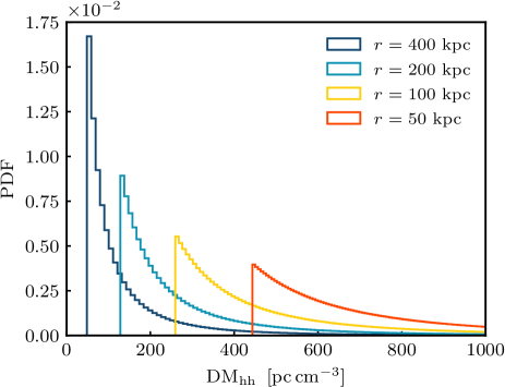
Can host halo DMs plausibly be of order ${\rm DM}_{\rm hh}\gtrsim 400$ pc cm^-3? To answer this question, in Figure 11, we show ${\rm DM}_{\rm hh}$ histograms for simulated FRBs in a halo of mass $M=10^{14}M_{\odot}$ . The halo gas profile is the intracluster medium (ICM) model from Prochaska & Zheng (2019), based on X-ray observations from Vikhlinin et al. (2006)⁷⁷7To calculate the host halo DM ${\rm DM}_{\rm hh}=\int dr\,n_{e}(r)$ , we used a slightly modified version of the FRB software (github.com/FRBs/FRB) by Prochaska et al. We thank the authors for making their software public.. It is seen that FRBs near the centers ( $r\lesssim 100$ kpc) of large ( $M\sim 10^{14}M_{\odot}$ ) halos can have host halo DMs ${\rm DM}_{\rm hh}\gtrsim 400$ pc cm^-3.

Thus, the high-DM signal in Figure 9 is plausibly explained by a small subpopulation of FRBs at redshift $0.3\lesssim z\lesssim 0.5$ near the centers of large halos. Such a subpopulation could have ${\rm DM}_{\rm host}\gtrsim 400$ pc cm^-3, and strongly correlate with galaxies, since bright galaxies are often in high-mass halos.

This mechanism is a proof of concept to show that ${\rm DM}_{\rm hh}\gtrsim 400$ pc cm^-3 is plausible in some halo gas models. Other mechanisms may also be possible, such as augmentation by intervening foreground galaxies (James et al., 2021b). We emphasize that the statistical evidence for a population of FRBs with ${\rm DM}_{\rm host}\gtrsim 400$ pc cm^-3, presented in the previous subsection, does not depend on the assumption of a particular model or mechanism.

4.4 Propagation effects

So far, we have assumed that the observed FRB-galaxy correlation is owing to spatial correlations between the FRB and galaxy populations. In this subsection, we will explore the alternate hypothesis that host DMs are always small (say ${\rm DM}_{\rm host}\sim 70$ pc cm^-3), and that propagation effects are responsible for the observed correlation between $z\sim 0.4$ galaxies and high-DM FRBs.

“Propagation effects” is a catch-all term for what happens to radio waves during their voyage from source and observer due to intervening plasma. For example, dispersion, scattering, and plasma lensing are all propagation effects. Propagation effects can produce an apparent correlation between low-redshift galaxies and high-redshift FRBs, even when the underlying populations are not spatially correlated.

For example, low-redshift galaxies are spatially correlated with free electrons, which contribute to the DM of background FRBs. The DM contribution can either increase or decrease the probability of detecting a background FRB, depending on the selection function of the instrument. This effect can produce an apparent correlation or anticorrelation between low- $z$ galaxies and high- $z$ FRBs, in the absence of any spatial correlation between the galaxy and FRB populations.

Here, we will calculate contributions to $C_{\ell}^{fg}$ from propagation effects, using formalism from Rafiei-Ravandi et al. (2020). We will use a fiducial model in which host DMs are small ( ${\rm DM}_{\rm host}\sim 70$ pc cm^-3), implying negligible spatial correlation between $z\sim 0.4$ galaxies and high-DM FRBs. This is because we are interested in exploring the hypothesis that propagation effects (not large host DMs) are entirely responsible for the observed DM dependence in Figure 9. We describe the fiducial model in the next few paragraphs.

First, we model the distribution of FRBs in redshift and DM. We assume that the FRB redshift distribution is

\frac{dn_{f}^{2d}}{dz}\propto z^{2}e^{-\gamma z}

(22)

and that the host DM distribution is lognormal, and independent of redshift:

p({\rm DM}_{\rm host})\propto\frac{1}{{\rm DM}_{\rm host}}\exp\left(-\frac{(\log{\rm DM}_{\rm host}-\mu_{\log})^{2}}{2\sigma_{\log}^{2}}\right)\,.

(23)

In Eqs. (22), (23), we choose parameters

\gamma=6.7\hskip 28.45274pt\mu_{\log}=4.2\hskip 28.45274pt\sigma_{\log}=5\,.

(24)

The total DM is ${\rm DM}={\rm DM}_{\rm IGM}(z)+{\rm DM}_{\rm host}$ . These parameters have been chosen so that the median FRB redshift is 0.4, the median host DM is 67 pc cm^-3, and the distribution of total DMs is similar to the observed DM distribution in Figure 12.

We will also need a fiducial model for $P_{ge}(k)$ , the 3D galaxy-electron power spectrum at comoving wavenumber $k$ . For reasons that we will explain shortly, we will need to know the one-halo contribution in the limit $k\rightarrow 0$ , which is (Rafiei-Ravandi et al., 2020)

\lim_{k\rightarrow 0}P_{ge}^{1h}(k,z)=\frac{\langle N_{e}^{\rm ion}\rangle}{n_{e,0}}\,,

(25)

where $\langle N_{e}^{\rm ion}\rangle$ is the average (over survey galaxies) number of electrons in the halo containing a galaxy, and $n_{e,0}$ is the comoving electron number density. To compute $\langle N_{e}^{\rm ion}\rangle$ , we assume that survey galaxies are contained in dark matter halos whose mass $M_{h}$ is lognormal-distributed, with parameters:

\big{\langle}\lambda\big{\rangle}=13.4\hskip 28.45274pt\sigma\big{(}\lambda\big{)}=0.35\,,

(26)

where $\lambda\equiv\log_{10}(M_{h}/M_{\odot})$ . This distribution is a rough fit to the halo mass distribution shown in Figure 3 of Schaan et al. (2021) for SDSS-LOWZ, a well-characterized $z\sim 0.3$ galaxy survey similar to the ones considered here. We assume that these large halos have baryon-to-matter ratio equal to the cosmic average $(\Omega_{b}/\Omega_{m})$ , with ionization fraction $f_{b}=0.75$ .

Finally, we model the CHIME/FRB selection function $S({\rm DM})$ in DM. This has been measured via Monte Carlo analysis of simulated events, and the result is shown in Figure 14 of the CHIME/FRB Catalog 1 paper (CHIME/FRB Collaboration, 2021). Here, we will use the following rough visual fit:

\log S({\rm DM})=0.1-0.14\left[\log\left(\frac{{\rm DM}}{1000}\right)\right]^{2}.

(27)

The selection function $S({\rm DM})$ is, up to normalization, the probability that a random FRB with a given DM is detected by CHIME/FRB. As an aside, CHIME/FRB has a selection bias against detecting high-DM FRBs due to frequency channel smearing and a bias against detecting low-DM FRBs due to the details of the high-pass filtering used in radio frequency interference removal. (Scattering biases will be discussed later in this section.) This combination of biases results in the selection function (Eq. 27) with a local maximum at ${\rm DM}\sim 1000$ pc cm^-3.

With the fiducial model in the previous few paragraphs, we now proceed to calculate contributions to $C_{\ell}^{fg}$ from propagation effects.

The first propagation effect we will consider is “DM-completeness”, described schematically as follows. Consider a foreground population of galaxies, and a background (i.e. higher-redshift) population of FRBs. The galaxies are spatially correlated with ionized electrons, which increase DMs of the FRBs, by adding dispersion along the line of sight. This can either increase or decrease the apparent number density of FRBs, depending on whether $dS/d({\rm DM})$ is positive or negative. This combination of effects produces a correlation between number densities of FRBs and galaxies, i.e. a contribution to $C_{\ell}^{fg}$ that can be positive or negative.

In Rafiei-Ravandi et al. (2020), the contribution to $C_{\ell}^{fg}$ from DM-completeness is calculated:

C_{\ell}^{fg}=\frac{1}{n_{g}^{2d}}\int dz\,\frac{H(z)}{\chi(z)^{2}}\frac{dn_{g}^{2d}}{dz}W_{f}(z)\,P_{ge}\bigg{(}\frac{\ell}{\chi(z)},z\bigg{)}\,,

(28)

where the DM-completeness weight function $W_{f}$ for DM bin $[{\rm DM}_{\rm min},{\rm DM}_{\rm max}]$ is

	$\displaystyle W_{f}(z)$	$\displaystyle=$	$\displaystyle\frac{n_{e,0}}{n_{f}^{2d}}\,\frac{1+z}{H(z)}\int_{z}^{\infty}dz^{\prime}$		(29)
			$\displaystyle\times\int_{{\rm DM}_{\rm min}}^{{\rm DM}_{\rm max}}d({\rm DM})\frac{d^{2}n^{2d}_{f}}{dz^{\prime}\,d({\rm DM})}\frac{d\log S}{d({\rm DM})}$		(29)

and $\chi(z)$ is comoving distance to redshift $z$ . We convert this expression for $C_{\ell}^{fg}$ to an expression for our parameter $\alpha$ as follows:

	$\displaystyle\alpha$	$\displaystyle=\lim_{\ell\rightarrow 0}C_{\ell}^{fg(1h)}$
		$\displaystyle=\frac{1}{n_{g}^{2d}}\int dz\,\frac{H(z)}{\chi(z)^{2}}\frac{dn_{g}^{2d}}{dz}W_{f}(z)\frac{\langle N_{e}^{\rm ion}(z)\rangle}{n_{e,0}}\,,$		(30)

where we have used Eq. (18) in the first line and Eqs. (25), (28) in the second line.

The second propagation effect we will consider is “DM-shifting”, which arises for an FRB catalog that has been binned in DM, as in Figure 9. Even in the absence of an instrumental selection function, DM fluctuations along the line of sight can shift FRBs across DM bin boundaries, either increasing or decreasing the observed number density of FRBs in a given bin. This effect is distinct from the DM-completeness effect described above, and also produces a contribution to $C_{\ell}^{fg}$ that can be positive or negative. Using results from Rafiei-Ravandi et al. (2020), the DM-shifting bias to $\alpha_{L}$ is given by the previous expression (30), but with the following expression for the DM-shifting weight function:

W_{f}(z)=-\frac{n_{e,0}}{n_{f}^{2d}}\,\frac{1+z}{H(z)}\int_{z}^{\infty}dz^{\prime}\left[\frac{d^{2}n_{f}^{2d}}{dz^{\prime}\,d({\rm DM})}\right]_{{\rm DM}_{\rm min}}^{{\rm DM}_{\rm max}}\,.

(31)

In Figure 13, we show $\alpha_{L}$ -biases from the DM-completeness and DM-shifting propagation effects in our fiducial model, computed using Eqs. (29)–(31). For simplicity, we have approximated the precise $z$ -dependence of the redshift-binned galaxy surveys in Figure 9 by assuming $dn_{g}^{2d}/dz=\mbox{const}$ for $0.3\leq z\leq 0.4$ . (The results are not very sensitive to the galaxy redshift distribution.)

Comparing to the FRB-galaxy correlation shown previously in Figure 9, we see that the total bias is $\sim 0.5\sigma$ in the second DM bin ( $262<{\rm DM}<393$ pc cm^-3), and $\lesssim 0.1\sigma$ in the other bins. These biases are too small, and have the wrong DM dependence, to explain the FRB-galaxy correlation shown previously in Figure 9.

So far, we have only considered propagation effects involving dispersion. The next propagation effect we might want to consider is scattering completeness, described intuitively as follows. Consider a foreground population of galaxies and a background population of FRBs. The galaxies are correlated with free electrons, which scatter-broaden FRBs and change their observed number density. Since scatter-broadening always decreases the probability that an FRB is detected, this effect always produces negative $C_{\ell}^{fg}$ .⁸⁸8Formally, the selection function for scattering is a decreasing function of scattering width. This can be seen directly in Figure 15 of (CHIME/FRB Collaboration, 2021). Therefore, scattering completeness cannot be responsible for the observed FRB-galaxy correlation, which is positive (as expected for clustering).

A final category of propagation effects is strong lensing (either plasma lensing or gravitational lensing) by foreground galaxies. Although strong lenses are rare, they can produce large magnification, increasing the detection rate of background FRBs by a large factor if the FRB luminosity function is sufficiently steep. A complete analysis of strong lensing in CHIME/FRB would be a substantial undertaking, and we defer it to a future paper.

5 Summary and conclusions

In this paper, we find a cross-correlation between CHIME FRBs and galaxies at redshifts $0.3\lesssim z\lesssim 0.5$ . The correlation is statistically significant in three galaxy surveys: WISE $\times$ SCOS, DESI-BGS, and DESI-LRG. The statistical significance of the detection in each survey is $p\sim 2.7\times 10^{-5}$ , $3.1\times 10^{-4}$ , and $4.1\times 10^{-4}$ , respectively. These $p\mkern 1.55mu$ -values account for look-elsewhere effects in both angular scale $L$ and redshift range.

The FRB-galaxy correlation is detected on angular scales ( $\ell\sim 1000$ ) in the one-halo regime. In this regime, the amplitude of the correlation is proportional to the mean “link count” $\eta$ of the FRB population, i.e. mean number of galaxies in the same halo as an FRB. Cross-correlating CHIME FRBs with $0.3\lesssim z\lesssim 0.5$ galaxies, we find $\eta$ of order unity.

This measurement of $\eta$ cannot be directly translated to the probability $p$ that an FRB is in the given redshift range. We can write $\eta=p\tilde{\eta}$ , where $\tilde{\eta}$ is the mean link count of FRBs in the redshift range. Formally, we measure $(p\tilde{\eta})$ but not the individual factors $p,\tilde{\eta}$ . However, in the bright galaxy surveys considered here, dark matter halos rarely contain more than a few catalog galaxies. We conclude that $\tilde{\eta}$ must be of order unity, implying that $p$ is also of order unity. That is, an order-one fraction of CHIME FRBs are in redshift range $0.3\lesssim z\lesssim 0.5$ .

We have phrased this conclusion as a qualitative statement (“order-one fraction”), since it is difficult to assign a quantitative upper bound to $\tilde{\eta}$ . This issue is a limitation of measuring FRB-galaxy correlations in the one-halo regime, where the FRB redshift distribution always appears multiplied by a linking factor $\tilde{\eta}$ . Future CHIME/FRB catalogs should contain enough FRBs to detect the FRB-galaxy correlation on two-halo scales ( $\ell\sim 100$ ) (Rafiei-Ravandi et al., 2020), which will help break this degeneracy.

We find statistical evidence for a population of FRBs with large host DMs, on the order of ${\rm DM}_{\rm host}\sim 400$ pc cm^-3. More precisely, we detect a nonzero correlation between FRBs with DM $\geq 785$ pc cm^-3 (after subtracting the YWM16 estimate of the Milky Way DM) and galaxies at $z\sim 0.4$ , where the IGM contribution to the DM is ${\rm DM}_{\rm IGM}(z)\sim 360$ pc cm^-3.

This may appear to be in tension with direct host galaxy associations. At the time of this writing, 14 FRBs have been localized to host galaxies, all of which have ${\rm DM}_{\rm host}\lesssim 200$ pc cm^-3. However, FRBs with DM $\geq 785$ pc cm^-3 are currently uncommon, and our FRB-galaxy correlation result must be interpreted carefully. It implies that an order-one fraction of high-DM FRBs are at redshift $z\sim 0.4$ in CHIME/FRB, but it does not imply that an order-one fraction of FRBs at redshift $z\sim 0.4$ have high DM. These statements are actually consistent with the direct associations. Since there is currently only one direct association with YMW16-subtracted DM $\geq 785$ pc cm^-3, one cannot currently rule out the possibility that an order-one fraction of high-DM FRBs are at $z\sim 0.4$ .

The number of direct host associations is rapidly growing, and we predict that direct associations will soon find high-DM FRBs with $z\sim 0.4$ . However, we note that most direct associations to date have been discovered by ASKAP at lower DM (on average) than the CHIME/FRB sample.

We briefly explore mechanisms for producing host DMs $\gtrsim 400$ pc cm^-3, and show that contributions from gas in large halos provide a plausible mechanism. Quantitatively, we find that for FRBs near the centers ( $r\lesssim 100$ kpc) of large ( $M\sim 10^{14}M_{\odot}$ ) halos the host halo DM can be $\gtrsim 400$ pc cm^-3 (Figure 11), at least in one widely used ICM model (Prochaska & Zheng, 2019). FRBs in such halos will strongly correlate with galaxies, since bright survey galaxies are often found in large halos. We show that line-of-sight propagation effects are unlikely to be a significant source of bias (§4.4).

Future measurements of FRB-galaxy cross-correlations will have higher SNR, and the results presented here could be extended in several ways. One could bin simultaneously in galaxy redshift and FRB DM, to explore the FRB-galaxy correlation strength as a function of two variables $(z,\mbox{DM})$ . Cross-correlations can constrain the high- $z$ tail of the FRB redshift distribution, where direct associations are difficult since individual galaxies are usually faint (Eftekhari & Berger, 2017). Very high- $z$ FRBs, if present, can be used to constrain cosmic reionization history (Caleb et al., 2019; Linder, 2020; Zhang et al., 2021). Finally, line-of-sight propagation effects will eventually be detectable in $C_{\ell}^{fg}$ , and will be an interesting probe of the distribution of electrons in the universe.

This paper is based on FRBs from CHIME/FRB Catalog 1, which contains 489 unique sources and approximate angular sky positions. Future CHIME/FRB catalogs will include more FRB sources, many of which will have improved angular resolution through use of baseband data (Michilli et al., 2021). The FRB-galaxy correlation presented here should have much higher statistical significance in future CHIME/FRB catalogs and will be exciting to explore.

We thank the Dominion Radio Astrophysical Observatory, operated by the National Research Council Canada, for gracious hospitality and expertise. CHIME is funded by a grant from the Canada Foundation for Innovation (CFI) 2012 Leading Edge Fund (Project 31170) and by contributions from the provinces of British Columbia, Québec and Ontario. The CHIME/FRB Project is funded by a grant from the CFI 2015 Innovation Fund (Project 33213), and by contributions from the provinces of British Columbia, Québec, and by the Dunlap Institute for Astronomy and Astrophysics at the University of Toronto. The Dunlap Institute is funded through an endowment established by the David Dunlap family and the University of Toronto. Additional support was provided by the Canadian Institute for Advanced Research (CIFAR), McGill University and the McGill Space Institute via the Trottier Family Foundation, and the University of British Columbia. Research at Perimeter Institute is supported by the Government of Canada through Industry Canada and by the Province of Ontario through the Ministry of Research & Innovation. K.M.S. was supported by an NSERC Discovery Grant and a CIFAR fellowship. K.W.M. is supported by an NSF grant (2008031). M.D. is supported by a Killam Fellowship, NSERC Discovery Grant, CIFAR, and by the FRQNT Centre de Recherche en Astrophysique du Québec (CRAQ). M.B. is supported by an FRQNT Doctoral Research Award. K. B. is supported by an NSF grant (2006548). P.C. is supported by an FRQNT Doctoral Research Award. B.M.G. is supported by an NSERC Discovery grant (RGPIN-2015-05948), and by the Canada Research Chairs (CRC) program. D.C.G is supported by the John I. Watters Research Fellowship. V.M.K. holds the Lorne Trottier Chair in Astrophysics & Cosmology, a Distinguished James McGill Professorship and receives support from an NSERC Discovery Grant (RGPIN 228738-13) and Gerhard Herzberg Award, from an R. Howard Webster Foundation Fellowship from CIFAR, and from the FRQNT CRAQ. C.L. was supported by the U.S. Department of Defense (DoD) through the National Defense Science & Engineering Graduate Fellowship (NDSEG) Program. J.M.-P is a Kavli Fellow. D.M. is a Banting Fellow. E.P. acknowledges funding from an NWO Veni Fellowship. P.S. is a Dunlap Fellow and an NSERC Postdoctoral Fellow. K.S. is supported by the NSF Graduate Research Fellowship Program. FRB research at UBC is supported by an NSERC Discovery Grant and by CIFAR. This research was enabled in part by support provided by WestGrid (www.westgrid.ca) and Compute Canada (www.computecanada.ca). The Photometric Redshifts for the Legacy Surveys (PRLS) catalog used in this paper was produced thanks to funding from the U.S. Department of Energy Office of Science, Office of High Energy Physics via grant DE-SC0007914.

References

Aghanim et al. (2020) Aghanim, N., Akrami, Y., Ashdown, M., et al. 2020, A&A, 641, A6, doi: 10.1051/0004-6361/201833910
Alonso (2021) Alonso, D. 2021, Physical Review D, 103, 123544, doi: 10.1103/PhysRevD.103.123544
Alonso et al. (2015) Alonso, D., Salvador, A. I., Sánchez, F. J., et al. 2015, Monthly Notices of the Royal Astronomical Society, 449, 670, doi: 10.1093/mnras/stv309
Balaguera-Antolínez et al. (2018) Balaguera-Antolínez, A., Bilicki, M., Branchini, E., & Postiglione, A. 2018, Monthly Notices of the Royal Astronomical Society, 476, 1050, doi: 10.1093/mnras/sty262
Bannister et al. (2019) Bannister, K. W., Deller, A. T., Phillips, C., et al. 2019, Science, 365, 565, doi: 10.1126/science.aaw5903
Bassa et al. (2017) Bassa, C. G., Tendulkar, S. P., Adams, E. A. K., et al. 2017, The Astrophysical Journal, 843, L8, doi: 10.3847/2041-8213/aa7a0c
Bhandari et al. (2020a) Bhandari, S., Sadler, E. M., Prochaska, J. X., et al. 2020a, The Astrophysical Journal, 895, L37, doi: 10.3847/2041-8213/ab672e
Bhandari et al. (2020b) Bhandari, S., Bannister, K. W., Lenc, E., et al. 2020b, The Astrophysical Journal, 901, L20, doi: 10.3847/2041-8213/abb462
Bhardwaj et al. (2021) Bhardwaj, M., Gaensler, B. M., Kaspi, V. M., et al. 2021, The Astrophysical Journal, 910, L18, doi: 10.3847/2041-8213/abeaa6
Bilicki et al. (2013) Bilicki, M., Jarrett, T. H., Peacock, J. A., Cluver, M. E., & Steward, L. 2013, The Astrophysical Journal Supplement Series, 210, 9, doi: 10.1088/0067-0049/210/1/9
Bilicki et al. (2016) Bilicki, M., Peacock, J. A., Jarrett, T. H., et al. 2016, The Astrophysical Journal Supplement Series, 225, 5, doi: 10.3847/0067-0049/225/1/5
Bochenek et al. (2020) Bochenek, C. D., Ravi, V., Belov, K. V., et al. 2020, Nature, 587, 59, doi: 10.1038/s41586-020-2872-x
Caleb et al. (2019) Caleb, M., Flynn, C., & Stappers, B. W. 2019, Monthly Notices of the Royal Astronomical Society, 485, 2281, doi: 10.1093/mnras/stz571
Chatterjee et al. (2017) Chatterjee, S., Law, C. J., Wharton, R. S., et al. 2017, Nature, 541, 58, doi: 10.1038/nature20797
CHIME/FRB Collaboration (2018) CHIME/FRB Collaboration. 2018, The Astrophysical Journal, 863, 48, doi: 10.3847/1538-4357/aad188
CHIME/FRB Collaboration (2019) —. 2019, The Astrophysical Journal, 885, L24, doi: 10.3847/2041-8213/ab4a80
CHIME/FRB Collaboration (2020a) —. 2020a, Nature, 587, 54, doi: 10.1038/s41586-020-2863-y
CHIME/FRB Collaboration (2020b) —. 2020b, Nature, 582, 351, doi: 10.1038/s41586-020-2398-2
CHIME/FRB Collaboration (2021) —. 2021, Submitted to ApJS
Chittidi et al. (2020) Chittidi, J. S., Simha, S., Mannings, A., et al. 2020, arXiv e-prints, arXiv:2005.13158. https://ui.adsabs.harvard.edu/abs/2020arXiv200513158C
Cooray & Sheth (2002) Cooray, A., & Sheth, R. 2002, Physics Reports, 372, 1, doi: 10.1016/s0370-1573(02)00276-4
Cordes & Chatterjee (2019) Cordes, J. M., & Chatterjee, S. 2019, Annual Review of Astronomy and Astrophysics, 57, 417, doi: 10.1146/annurev-astro-091918-104501
Cordes & Lazio (2002) Cordes, J. M., & Lazio, T. J. W. 2002, arXiv e-prints, astro. https://ui.adsabs.harvard.edu/abs/2002astro.ph..7156C
Dey et al. (2019) Dey, A., Schlegel, D. J., Lang, D., et al. 2019, The Astronomical Journal, 157, 168, doi: 10.3847/1538-3881/ab089d
Eftekhari & Berger (2017) Eftekhari, T., & Berger, E. 2017, The Astrophysical Journal, 849, 162, doi: 10.3847/1538-4357/aa90b9
Gorski et al. (2005) Gorski, K. M., Hivon, E., Banday, A. J., et al. 2005, The Astrophysical Journal, 622, 759, doi: 10.1086/427976
Heintz et al. (2020) Heintz, K. E., Prochaska, J. X., Simha, S., et al. 2020, The Astrophysical Journal, 903, 152, doi: 10.3847/1538-4357/abb6fb
Hodges (1958) Hodges, J. L. 1958, Ark. Mat., 3, 469, doi: 10.1007/BF02589501
James et al. (2021a) James, C. W., Prochaska, J. X., Macquart, J. P., et al. 2021a, arXiv e-prints, arXiv:2101.07998. https://ui.adsabs.harvard.edu/abs/2021arXiv210107998J
James et al. (2021b) —. 2021b, arXiv e-prints, arXiv:2101.08005. https://ui.adsabs.harvard.edu/abs/2021arXiv210108005J
Josephy et al. (2021) Josephy, A., Chawla, P., Curtin, A. P., et al. 2021, Submitted to ApJ
Keating & Pen (2020) Keating, L. C., & Pen, U.-L. 2020, Monthly Notices of the Royal Astronomical Society: Letters, 496, L106, doi: 10.1093/mnrasl/slaa095
Kokubo et al. (2017) Kokubo, M., Mitsuda, K., Sugai, H., et al. 2017, The Astrophysical Journal, 844, 95, doi: 10.3847/1538-4357/aa7b2d
Krakowski et al. (2016) Krakowski, T., Małek, K., Bilicki, M., et al. 2016, A&A, 596. https://doi.org/10.1051/0004-6361/201629165
Law et al. (2020) Law, C. J., Butler, B. J., Prochaska, J. X., et al. 2020, The Astrophysical Journal, 899, 161, doi: 10.3847/1538-4357/aba4ac
Li et al. (2019) Li, D., Yalinewich, A., & Breysse, P. C. 2019, arXiv e-prints, arXiv:1902.10120
Linder (2020) Linder, E. V. 2020, Physical Review D, 101, 103019, doi: 10.1103/PhysRevD.101.103019
Macquart et al. (2020) Macquart, J. P., Prochaska, J. X., McQuinn, M., et al. 2020, Nature, 581, 391, doi: 10.1038/s41586-020-2300-2
Madhavacheril et al. (2019) Madhavacheril, M. S., Battaglia, N., Smith, K. M., & Sievers, J. L. 2019, Physical Review D, 100, 103532, doi: 10.1103/PhysRevD.100.103532
Mannings et al. (2021) Mannings, A. G., Fong, W.-f., Simha, S., et al. 2021, The Astrophysical Journal, 917, 75, doi: 10.3847/1538-4357/abff56
Marcote et al. (2020) Marcote, B., Nimmo, K., Hessels, J. W. T., et al. 2020, Nature, 577, 190, doi: 10.1038/s41586-019-1866-z
Masui & Sigurdson (2015) Masui, K. W., & Sigurdson, K. 2015, Physical Review Letters, 115, 121301, doi: 10.1103/PhysRevLett.115.121301
McQuinn (2014) McQuinn, M. 2014, The Astrophysical Journal Letters, 780, L33, doi: 10.1088/2041-8205/780/2/l33
Michilli et al. (2021) Michilli, D., Masui, K. W., Mckinven, R., et al. 2021, The Astrophysical Journal, 910, 147, doi: 10.3847/1538-4357/abe626
Navarro et al. (1997) Navarro, J. F., Frenk, C. S., & White, S. D. M. 1997, Astrophys. J., 490, 493, doi: 10.1086/304888
Petroff et al. (2019) Petroff, E., Hessels, J. W. T., & Lorimer, D. R. 2019, Astronomy and Astrophysics Review, 27, 4, doi: 10.1007/s00159-019-0116-6
Petroff & Yaron (2020) Petroff, E., & Yaron, O. 2020, Transient Name Server AstroNote, 160, 1
Platts et al. (2019) Platts, E., Weltman, A., Walters, A., et al. 2019, Physics Reports, 821, 1, doi: 10.1016/j.physrep.2019.06.003
Prochaska & Zheng (2019) Prochaska, J. X., & Zheng, Y. 2019, Monthly Notices of the Royal Astronomical Society, 485, 648, doi: 10.1093/mnras/stz261
Prochaska et al. (2019) Prochaska, J. X., Macquart, J.-P., McQuinn, M., et al. 2019, Science, 366, 231, doi: 10.1126/science.aay0073
Rafiei-Ravandi et al. (2020) Rafiei-Ravandi, M., Smith, K. M., & Masui, K. W. 2020, Physical Review D, 102, 023528, doi: 10.1103/PhysRevD.102.023528
Raichoor et al. (2020) Raichoor, A., Eisenstein, D. J., Karim, T., et al. 2020, Research Notes of the American Astronomical Society, 4, 180, doi: 10.3847/2515-5172/abc078
Ravi et al. (2019) Ravi, V., Catha, M., D’Addario, L., et al. 2019, Nature, 572, 352, doi: 10.1038/s41586-019-1389-7
Reischke et al. (2021a) Reischke, R., Hagstotz, S., & Lilow, R. 2021a, Physical Review D, 103, 023517, doi: 10.1103/PhysRevD.103.023517
Reischke et al. (2021b) —. 2021b, arXiv e-prints, arXiv:2102.11554. https://ui.adsabs.harvard.edu/abs/2021arXiv210211554R
Ruiz-Macias et al. (2020) Ruiz-Macias, O., Zarrouk, P., Cole, S., et al. 2020, Research Notes of the American Astronomical Society, 4, 187, doi: 10.3847/2515-5172/abc25a
Schaan et al. (2021) Schaan, E., Ferraro, S., Amodeo, S., et al. 2021, Physical Review D, 103, 063513, doi: 10.1103/PhysRevD.103.063513
Scholz & Stephens (1987) Scholz, F. W., & Stephens, M. A. 1987, Journal of the American Statistical Association, 82, 918, doi: 10.1080/01621459.1987.10478517
Shirasaki et al. (2017) Shirasaki, M., Kashiyama, K., & Yoshida, N. 2017, Physical Review D, 95, 083012, doi: 10.1103/PhysRevD.95.083012
Simha et al. (2020) Simha, S., Burchett, J. N., Prochaska, J. X., et al. 2020, The Astrophysical Journal, 901, 134, doi: 10.3847/1538-4357/abafc3
Spanakis-Misirlis (2021) Spanakis-Misirlis, A. 2021, Astrophysics Source Code Library, ascl:2106.028. https://ui.adsabs.harvard.edu/abs/2021ascl.soft06028S
Spitler et al. (2016) Spitler, L. G., Scholz, P., Hessels, J. W. T., et al. 2016, Nature, 531, 202, doi: 10.1038/nature17168
Tendulkar et al. (2017) Tendulkar, S. P., Bassa, C. G., Cordes, J. M., et al. 2017, The Astrophysical Journal, 834, L7, doi: 10.3847/2041-8213/834/2/l7
Vikhlinin et al. (2006) Vikhlinin, A., Kravtsov, A., Forman, W., et al. 2006, The Astrophysical Journal, 640, 691, doi: 10.1086/500288
Wechsler & Tinker (2018) Wechsler, R. H., & Tinker, J. L. 2018, Annual Review of Astronomy and Astrophysics, 56, 435, doi: 10.1146/annurev-astro-081817-051756
Yao et al. (2017) Yao, J. M., Manchester, R. N., & Wang, N. 2017, The Astrophysical Journal, 835, 29, doi: 10.3847/1538-4357/835/1/29
Zhang et al. (2021) Zhang, Z. J., Yan, K., Li, C. M., Zhang, G. Q., & Wang, F. Y. 2021, The Astrophysical Journal, 906, 49, doi: 10.3847/1538-4357/abceb9
Zhou et al. (2020a) Zhou, R., Newman, J. A., Mao, Y.-Y., et al. 2020a, Monthly Notices of the Royal Astronomical Society, doi: 10.1093/mnras/staa3764
Zhou et al. (2020b) Zhou, R., Newman, J. A., Dawson, K. S., et al. 2020b, Research Notes of the American Astronomical Society, 4, 181, doi: 10.3847/2515-5172/abc0f4

Appendix A Statistical errors on FRB locations

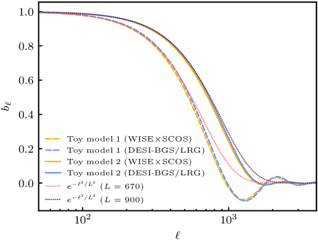
Statistical errors in CHIME/FRB sky locations suppress the FRB-galaxy power spectrum $C_{\ell}^{fg}$ on small scales (large $\ell$ ). The suppression takes the form $C_{\ell}^{fg}\rightarrow b_{\ell}C_{\ell}^{fg}$ , where $b_{\ell}$ is the “beam” transfer function. Throughout the paper, we have modeled statistical errors as Gaussian, which leads to a transfer function of the form $b_{\ell}=e^{-\ell^{2}/L^{2}}$ .

In this appendix, we will study statistical errors in more detail, using toy models of the CHIME/FRB instrument and the FRB population. Our conclusions are as follows:

•

Statistical errors are not strictly Gaussian, but a Gaussian transfer function $b_{\ell}=e^{-\ell^{2}/L^{2}}$ is a good approximation within the error bars of our $C_{\ell}^{fg}$ measurement.
•

Calculating $L$ from first principles is hard, since it depends on both the CHIME/FRB instrument and the FRB population. A plausible range of $L$ -values is $315\leq L\leq 1396$ .

This justifies the methodology used throughout the paper, where a Gaussian transfer function $b_{\ell}=e^{-\ell^{2}/L^{2}}$ is used, but $L$ is a free parameter that we fit to the data, varying $L$ over the range $315\leq L\leq 1396$ .

A.1 Toy beam model 1: uniform density, center of nearest beam

CHIME FRBs are detected by searching a $4\times 256$ regular array of formed beams independently in real time. A best-fit sky location is assigned to each detected FRB based on the detection SNR (or nondetection) in each beam, using the localization pipeline described by CHIME/FRB Collaboration (2019, 2021). For an FRB which is detected in a single beam, the localization pipeline assigns sky location equal to the beam center. For a multibeam detection, the assigned sky location is roughly a weighted average of the beams where the event was detected.

As a first attempt to model statistical errors in the localization pipeline, suppose that when an FRB is detected we assign it to the center of the closest FRB beam. This is a reasonable model for the single-beam detections as described above.

We neglect wavelength dependence of the beam and evaluate at central wavelength $\lambda=0.5$ m. We also neglect FRBs in sidelobes of the primary beam, since these are a small fraction of the CHIME/FRB Catalog 1. Finally, we assume that FRBs detected by CHIME/FRB are uniformly distributed over the sky. (This turns out to be a dubious approximation, as we will show in the next subsection.) What is $b_{\ell}$ in this toy model?

Let $\Theta_{e}$ be the elevation of the detected FRB (with the usual astronomical definition, i.e. $\Theta_{e}=0$ for an FRB on the horizon, or $\Theta_{e}=\pi/2$ for an FRB at zenith). Let $\theta_{x},\theta_{y}$ be east-west and north-south sky coordinates in a coordinate system where the center of the formed beam is at $(0,0)$ . Let $S$ be the set of points closer to $(0,0)$ than any of the other beam centers:

S=\left[-\frac{\theta_{0}}{2},\frac{\theta_{0}}{2}\right]\times\left[-\frac{\theta_{0}}{2\sin\Theta_{e}},\frac{\theta_{0}}{2\sin\Theta_{e}}\right]\,,

(A1)

where $\theta_{0}=23\farcm 4$ in CHIME. If the detected FRBs are uniformly distributed on the sky, then the effective beam is

b_{\ell}=\frac{\int_{S}d^{2}\theta\,J_{0}(\ell\theta)}{\int_{S}d^{2}\theta\,1}\,,

(A2)

where $J_{0}(x)$ is a Bessel function. For the CHIME/FRB catalog, which contains FRBs with different elevations $\Theta_{e}$ , we average $b_{\ell}$ over $\Theta_{e}$ values in the catalog. It is straightforward to compute the elevation $\Theta_{e}$ for each FRB, using values of RA, Dec, and time of observation taken directly from the catalog. The resulting transfer function $b_{\ell}$ is shown in Figure 14, and agrees well with a Gaussian transfer function $b_{\ell}=e^{-\ell^{2}/L^{2}}$ with $L=670$ .

A.2 Toy beam model 2: including selection bias

In the previous subsection, we neglected a selection bias: an FRB is more likely to be detected if it is located at the center of the beam (where the instrumental response is largest). To account for this selection bias, we define the unnormalized intensity beam:

B(\theta_{x},\theta_{y})=\frac{\mbox{sinc}^{2}(\theta_{x}D_{x}/\lambda)\,\mbox{sinc}^{2}((\theta_{y}D_{y}\sin\Theta_{e})/\lambda)}{\mbox{sinc}^{2}(\theta_{x}D_{x}/4\lambda)}\,,

(A3)

where $\theta_{x},\theta_{y},\Theta_{e},\lambda$ are defined in §A.1, the CHIME aperture is modeled as a rectangle with dimensions $(D_{x},D_{y})=(80,100)$ meters, and $\mbox{sinc}(x)=\sin(\pi x)/(\pi x)$ .

Assuming a Euclidean FRB fluence distribution $N(\geq F)\propto F^{-3/2}$ (consistent with statistical analysis of the CHIME/FRB Catalog 1 (CHIME/FRB Collaboration, 2021)), the probability of detecting an FRB at sky location $(\theta_{x},\theta_{y})$ is $\propto B(\theta_{x},\theta_{y})^{3/2}$ . Therefore, the beam transfer function is

b_{\ell}=\frac{\int_{S}d^{2}\theta\,B(\theta)^{3/2}J_{0}(\ell\theta)}{\int_{S}d^{2}\theta\,B(\theta)^{3/2}}

(A4)

averaged over catalog elevations $\Theta_{e}$ as in the previous subsection. The resulting transfer function $b_{\ell}$ is shown in Figure 14 and agrees well with a Gaussian transfer function $b_{\ell}=e^{-\ell^{2}/L^{2}}$ with $L=900$ .

A.3 Plausible range of $L$ -values

Comparing the last two subsections, we see that the selection bias considered in §A.2 increases the effective value of $L$ by 34%. This treatment of selection bias is incomplete, and a full study is outside the scope of this paper. For example, $b_{\ell}$ depends on wavelength $\lambda$ , so there is a selection bias involving FRB frequency spectra. In addition, we have not attempted to model multibeam detections, which will be better localized than single-beam detections. Given these sources of modeling uncertainty, rather than trying to model the value of $L$ precisely, we will assign a range of plausible $L$ -values.

To assign a smallest plausible $L$ -value, we make assumptions that lead to the largest plausible localization errors. We start with the toy beam model $b_{\ell}$ from §A.2, with $\lambda=0.75$ m (the longest wavelength in CHIME). We then convolve with a halo profile ( $b_{\ell}\rightarrow b_{\ell}u_{\ell}(M,z)^{2}$ , where $u_{\ell}(M,z)$ is a Navarro-Frenk-White (NFW) density profile; Navarro et al., 1997), taking the halo mass $M$ to be large ( $M=10^{14.5}~{}h^{-1}M_{\odot}$ ) and the redshift to be small ( $z=0.05$ ). These specific values are somewhat arbitrary, but the goal is to establish a baseline plausible value of $L_{\rm min}$ , not model a precise value of $L$ . With the assumptions in this paragraph, we get $L_{\rm min}=315$ .

Similarly, to assign a largest plausible $L$ -value, we make assumptions that lead to the smallest plausible localization errors. We use the smallest toy model from §A.2 with $\lambda=0.375$ m (the shortest wavelength in CHIME). We assume that 40% of the events are multibeam detections, and that multibeam detections have localization errors that are smaller by a factor 3. As in the previous section, these specific values are somewhat arbitrary, but the goal is to establish a baseline plausible value of $L_{\rm max}$ , not model a precise value of $L$ . With the assumptions in this paragraph, we get $L_{\rm max}=1396$ .

Appendix B Null tests

As a general check for robustness of our FRB-galaxy correlation $C_{\ell}^{fg}$ , we would like to check that $C_{\ell}^{fg}$ does not depend on external variables, for example time of day (TOD). Our methodology for doing this is as follows. We divide the FRB catalog into low-TOD and high-TOD subcatalogs, cross-correlate each subcatalog with a galaxy sample, and compute the difference power spectrum:

d{\hat{C}}_{\ell}^{fg}\equiv{\hat{C}}_{\ell}^{fg\,({\rm low})}-{\hat{C}}_{\ell}^{fg\,({\rm high})}\,.

(B1)

Recall that for a non-null power spectrum ${\hat{C}}_{\ell}$ , we compressed the $\ell$ -dependence into a scalar summary statistic $\hat{\alpha}_{L}$ by taking a weighted $\ell$ -average (Eq. 11). Analogously, we compress the difference spectrum $d{\hat{C}}_{\ell}^{fg}$ into a summary statistic $\hat{\beta}_{L}$ , defined by

\hat{\beta}_{L}=\sum_{\ell\geq\ell_{\rm min}}(2\ell+1)\frac{e^{-\ell^{2}/L^{2}}}{C_{\ell}^{gg}}d{\hat{C}}_{\ell}^{fg}\,,

(B2)

where $L$ is an angular scale parameter. Next, by analogy with ${\rm SNR}_{L}$ (defined previously in Eq. 14), we define

\Delta_{L}=\frac{\hat{\beta}_{L}}{\mbox{Var}(\hat{\beta}_{L})^{1/2}}\,.

(B3)

The value of $\Delta_{L}$ quantifies consistency (in “sigmas”) between $C_{\ell}^{fg}$ for the low-TOD and high-TOD subcatalogs.

We fix $L=1000$ , and consider three choices of galaxy catalog: WISE $\times$ SCOS with $z\geq 0.3125$ , DESI-BGS with $z\geq 0.295$ , and DESI-LRG with $z\leq 0.485$ . These redshift ranges are “cherry-picked” to maximize the FRB-galaxy cross-correlation (see Figure 7), but this cherry-picking should not bias the difference statistic $\Delta_{L}$ . With these choices, we find $\Delta_{L}=\{1.22,-0.21,1.30\}$ for WISE $\times$ SCOS, DESI-BGS, and DESI-LRG respectively. Therefore, there is no statistical evidence for dependence of $C_{\ell}^{fg}$ on time of day, since a 1.22 $\sigma$ , 0.21 $\sigma$ , or 1.30 $\sigma$ result is not statistically significant.

This test can be generalized by splitting on a variety of external variables (besides TOD). In Table 3, we identify 12 such variables and denote the corresponding $\Delta_{L}$ values (with $L=1000$ ) by $\Delta_{i}$ , where $i\in\{1,2,3,\dots,12\}$ . We note that these 12 tests are nonindependent, for example SNR is correlated with fluence. We also note that for many of these tests detection of a nonzero difference spectrum $d{\hat{C}}_{\ell}^{fg}$ does not necessarily indicate a problem. For example, DM dependence of $C_{\ell}^{fg}$ is expected at some level, since $C_{\ell}^{fg}$ is redshift dependent, and DM is correlated with redshift.

Parameter	Median	$\Delta_{i}$	Median	$\Delta_{i}$
	(WISE $\times$ SCOS)	WISE $\times$ SCOS	(DESI)	DESI-BGS	DESI-LRG
DM [pc cm^-3]	535.08	0.33	536.41	$-1.68$	$-0.95$
SNR	20.2	0.58	20.2	$0.00$	0.42
Scattering time [ms]	1.331	1.49	1.423	0.93	0.38
Pulse width [ms]	0.988	0.59	1.052	0.99	0.24
Spectral index	2.866	0.68	2.075	0.76	$-0.25$
Fluence [Jy ms]	3.503	1.28	3.115	$-1.00$	2.16
Bandwidth [MHz]	332.09	$-0.44$	358.09	0.80	1.58
Galactic $\|b\|$	38 $\fdg$ 26	0.59	38 $\fdg$ 24	$-1.27$	$-1.95$
Catalog localization error	10 $\farcm$ 12	0.52	9 $\farcm$ 53	2.16	1.19
${\rm TOA}-58528$ [MJD]	0.3686595	0.99	4.8473498	1.16	0.63
Peak frequency [MHz]	463.525	$-0.63$	449.036	1.97	1.30
Time of day [hr]	9.887	1.22	10.132	$-0.21$	1.30

Table 3: Null tests in Appendix B. For each parameter, we split the FRB catalog into “low” and “high” subcatalogs by comparing the parameter value to its median. (The median value is slightly different for FRBs in the WISE

\times

SCOS and DESI footprints.) We correlate both subcatalogs with the galaxy surveys, and compute the statistic

\Delta=(\Delta_{L})_{L=1000}

(defined in Eq. B3), which measures consistency of the FRB-galaxy correlation in “sigmas”.

There are a few $\sim$ 2 $\sigma$ outliers in Table 3, but a few outliers are unsurprising, so it is not immediately clear whether the $\Delta_{i}$ values in Table 3 are statistically different from zero. To answer this question, we reduce the 12-component vector $\Delta_{i}$ into a scalar summary statistic, in a few different ways as follows.

Our first summary statistic is intended to test whether the most anomalous $\Delta_{i}$ -value in each column of Table 3 is statistically significant. We define

\Delta_{\rm max}=\max_{i}|\Delta_{i}|\,.

(B4)

We then compare these values of $\Delta_{\rm max}$ to an ensemble of mocks. The mocks are constructed by randomizing the RA of each FRB in the catalog, keeping all other FRB properties (DM, SNR, etc.) fixed. This preserves any correlations which may be present between FRB properties. In the special case of the $|b|\geq 17^{\circ}$ null test, we recompute the value of $b$ after randomizing RA.

In Table 4, we report the $p\mkern 1.55mu$ -value for each $\Delta_{\rm max}$ , i.e. the fraction of mocks whose $\Delta_{\rm max}$ exceeds the “data” value. No statistically significant deviation from $\Delta_{\rm max}=0$ is seen.

Our second summary statistic is intended to test whether the 12-component vector $\Delta_{i}$ is consistent with a multivariate Gaussian distribution. We define:

\chi^{2}=\sum_{i,i^{\prime}}\Delta_{i}\,\mbox{Cov}\left(\Delta_{i},\Delta_{i^{\prime}}\right)^{-1}\Delta_{i^{\prime}}\,,

(B5)

where the covariance $\mbox{Cov}(\Delta_{i},\Delta_{i^{\prime}})$ is estimated from mock FRB catalogs, constructed as described above.

As before, to assign statistical significance, we compare the “data” value of $\chi^{2}$ to an ensemble of mocks and report the associated $p\mkern 1.55mu$ -value in Table 4. We find borderline evidence for $\chi^{2}\neq 0$ for DESI-BGS ( $p=0.030$ ), but interpret this as inconclusive, since Table 4 contains six $p\mkern 1.55mu$ -values, so one $p\mkern 1.55mu$ -value as small as 0.03 is unsurprising (this happens with probability $\approx$ 0.18).

Galaxy sample	$\Delta_{\rm max}$	$p\mkern 1.55mu$ -value	$\chi^{2}$	$p\mkern 1.55mu$ -value	KS $p\mkern 1.55mu$ -value	AD $p\mkern 1.55mu$ -value
WISE ${\times}$ SCOS	1.49	0.779	9.26	0.659	0.037	0.067
DESI-BGS	2.16	0.270	22.96	0.030	0.381	0.250
DESI-LRG	2.16	0.274	17.26	0.145	0.113	0.171

Table 4: Summary statistics for the 12 null tests in Table 3. As described in Appendix B, we reduce the 12-component vector

\Delta_{i}

into two scalar summary statistics

\Delta_{\rm max},\chi^{2}

, shown in the first four columns along with associated

p\mkern 1.55mu

-values from an ensemble of mocks. The last two columns compare the

\Delta_{i}

values for each galaxy sample to a “jackknife” ensemble defined by randomly splitting the CHIME/FRB catalog.

Finally, we compare the set of 12 $\Delta_{i}$ values to a jackknife distribution, obtained by randomly splitting the FRB catalog in half. We do this comparison using the 2-sample Kolmogorov-Smirnov (KS, Hodges, 1958) and Anderson-Darling (AD, Scholz & Stephens, 1987) tests. Figure 15 compares the two distributions for the three galaxy samples, and the last two columns of Table 4 summarize our results. As in the previous paragraph, there is one outlier: the WISE $\times$ SCOS KS $p\mkern 1.55mu$ -value is 0.037, which we interpret as inconclusive, since it is one out of six $p\mkern 1.55mu$ -values in the table (as in the previous paragraph).

Summarizing this appendix, we do not find statistically significant evidence that the FRB-galaxy clustering signal studied in this paper depends on any of the parameters in Table 3.

Appendix C Tail-fitting procedure

In §3.5, we assign statistical significance of the FRB-galaxy detection, by defining a frequentist statistic ${\rm SNR}_{\rm max}$ , and ranking the “data” value ${\rm SNR}_{\rm max}^{(\rm data)}$ within a histogram of simulated values ${\rm SNR}_{\rm max}^{(\rm mock)}$ . This procedure is conceptually straightforward, but there is a technical challenge: because ${\rm SNR}_{\rm max}^{(\rm data)}$ turns out to be an extreme outlier, a brute-force approach requires an impractical number of simulations. Therefore, we fit the tail of the ${\rm SNR}_{\rm max}^{(\rm mock)}$ distribution to an analytic distribution and assign statistical significance (or $p\mkern 1.55mu$ -value) analytically.

Empirically, we find that the top 10% of the ${\rm SNR}_{\rm max}^{(\rm mock)}$ distribution agrees well with the top 10% of a Gaussian distribution, as shown in Figure 16. The parameters of the Gaussian distribution were determined as follows. Let $p(x|\mu,\sigma)$ denote a Gaussian distribution with mean $\mu$ and variance $\sigma^{2}$ :

p(x|\mu,\sigma)=\frac{1}{\sigma\sqrt{2\pi}}e^{-(x-\mu)^{2}/(2\sigma^{2})}\,.

(C1)

Let $\Sigma_{+}\subset\mathbb{R}$ be the top 10% of the simulated ${\rm SNR}_{\rm max}^{(\rm mock)}$ values, and let $\Sigma_{-}$ be the bottom 90%. Let $\Sigma_{0}\in\mathbb{R}$ be the 90th percentile of the ${\rm SNR}_{\rm max}^{(\rm mock)}$ distribution. Then, we choose parameters $(\mu,\sigma)$ to maximize the likelihood function:

	$\displaystyle\log\mathcal{L}(x\|\mu,\sigma)$	$\displaystyle=\bigg{(}\sum_{x\in\Sigma_{+}}\log p(x\|\mu,\sigma)\bigg{)}$
		$\displaystyle\hskip 26.74565pt+\big{\|}\Sigma_{-}\big{\|}\log\int_{-\infty}^{\Sigma_{0}}p(x\|\mu,\sigma)\,,$		(C2)

where $x$ denotes mock realizations. This likelihood function has been constructed to fit parameters to the details of the $\Sigma_{+}$ values, while putting all $\Sigma_{-}$ values into a single coarse bin.

Figure 16 is a good visual test for goodness of fit, but as a more quantitative test, we compare the upper 10% of the simulated histogram with the Gaussian fit using a KS test. We find that the two distributions agree to $1\sigma$ (and likewise for the other two cases, DESI-BGS and DESI-LRG).

In Table 5, we compute statistical significance for each of the three surveys, in two different ways. The “brute-force” $p\mkern 1.55mu$ -value is obtained by counting the number of simulated ${\rm SNR}_{\rm max}^{(\rm mock)}$ values (out of $10^{4}$ total simulations) that exceed ${\rm SNR}_{\rm max}^{(\rm data)}$ . The “analytic” $p\mkern 1.55mu$ -value is obtained by fitting the top 10% of the simulated ${\rm SNR}_{\rm max}^{(\rm mock)}$ values to a Gaussian distribution, as described above, and evaluating the CDF of the distribution at ${\rm SNR}_{\rm max}^{(\rm data)}$ . The brute-force values are either uninformative (for WISE $\times$ SCOS), or have large Poisson uncertainties (for the other two surveys), so we have quoted the analytic $p\mkern 1.55mu$ -values as our “bottom-line” detection significances throughout the paper.

Survey	Brute-force	Analytic
WISE $\times$ SCOS	0/10000	$2.7\times 10^{-5}$
DESI-BGS	4/10000	$3.1\times 10^{-4}$
DESI-LRG	5/10000	$4.1\times 10^{-4}$

Table 5: “Brute-force” and analytic

p\mkern 1.55mu

-values, computed as described in Appendix C.

	$\displaystyle\log\mathcal{L}(x\|\mu,\sigma)$	$\displaystyle=\bigg{(}\sum_{x\in\Sigma_{+}}\log p(x\|\mu,\sigma)\bigg{)}$
		$\displaystyle\hskip 26.74565pt+\big{\|}\Sigma_{-}\big{\|}\log\int_{-\infty}^{\Sigma_{0}}p(x\|\mu,\sigma)\,,$		(C2)