The First CHIME/FRB Fast Radio Burst Catalog

Abstract

We present a catalog of 536 fast radio bursts (FRBs) detected by the Canadian Hydrogen Intensity Mapping Experiment Fast Radio Burst (CHIME/FRB) Project between 400 and 800 MHz from 2018 July 25 to 2019 July 1, including 62 bursts from 18 previously reported repeating sources. The catalog represents the first large sample, including bursts from repeaters and non-repeaters, observed in a single survey with uniform selection effects. This facilitates comparative and absolute studies of the FRB population. We show that repeaters and apparent non-repeaters have sky locations and dispersion measures (DMs) that are consistent with being drawn from the same distribution. However, bursts from repeating sources differ from apparent non-repeaters in intrinsic temporal width and spectral bandwidth. Through injection of simulated events into our detection pipeline, we perform an absolute calibration of selection effects to account for systematic biases. We find evidence for a population of FRBs—comprising a large fraction of the overall population—with a scattering time at 600 MHz in excess of 10 ms, of which only a small fraction are observed by CHIME/FRB. We infer a power-law index for the cumulative fluence distribution of $\alpha=-1.40\pm 0.11(\textrm{stat.})^{+0.06}_{-0.09}(\textrm{sys.})$, consistent with the $-3/2$ expectation for a non-evolving population in Euclidean space. We find $\alpha$ is steeper for high-DM events and shallower for low-DM events, which is what would be expected when DM is correlated with distance. We infer a sky rate of $[525\pm 30(\textrm{stat.})^{+140}_{-130}({\textrm{sys.}})]/\textrm{sky}/\textrm{day}$ above a fluence of 5 Jy ms at 600 MHz, with scattering time at $600$ MHz under 10 ms, and DM above 100 pc cm^-3.

1 Introduction

Although the first Fast Radio Burst (FRB) was discovered nearly a decade and a half ago (Lorimer et al., 2007), the nature of these sources remains a mystery. Now securely determined to originate from external galaxies, generally from cosmological distances (e.g., Tendulkar et al., 2017; Macquart et al., 2020), FRBs inhabit a unique and extreme portion of radio luminosity/time scale phase space (e.g., Cordes & Chatterjee, 2019) compared to other radio transients and hence are of great interest. Moreover, all-sky rates of $\sim 10^{3}$ per day (Bhandari et al., 2018) indicate that the phenomenon is ubiquitous. The mystery of FRBs therefore signals a common cosmic phenomenon borne from extreme, unknown environments.

One major clue regarding the nature of FRBs is that some repeat (Spitler et al., 2016), with periodic activity observed in two sources (CHIME/FRB Collaboration et al., 2020a; Rajwade et al., 2020). Repetition rules out cataclysmic models for at least the repeating FRB sources, though it remains unclear whether all FRBs are repeating sources that come with vastly different waiting times between repetitions (Ravi, 2019; James et al., 2020). Evidence for distinct emission phenomena has come from repeat bursts being wider than those from apparent non-repeaters (Scholz et al., 2016; CHIME/FRB Collaboration et al., 2019a; Fonseca et al., 2020). Additionally, the two localized repeating FRBs whose hosts have measured properties (Chatterjee et al., 2017; Marcote et al., 2020) are in late-type galaxies that have star formation, whereas localizations of apparent non-repeaters indicate these latter sources can sometimes reside in galaxies with modest or little star formation (Bhandari et al., 2020). To date, one Galactic magnetar has shown both repeated X-ray bursts and a radio burst of luminosity close to the FRB range (CHIME/FRB Collaboration et al., 2020b; Bochenek et al., 2020). This suggests that repeaters may be young, active magnetars, a scenario consistent with localizations of repeating FRBs to star-forming locations (Chatterjee et al., 2017; Marcote et al., 2020). Volumetric rate comparisons between FRBs and giant magnetar flares have been used to support the magnetar scenario (e.g., CHIME/FRB Collaboration et al., 2020b); however, uncertainties in current rate estimates are large, being dominated by either small number statistics or by systematics from including multiple different surveys having distinct biases. Detailed studies of a larger sample of FRBs from a single survey, repeating or not, are clearly of great value.

A detailed study of large numbers of FRBs, in a single homogeneous survey with a well-measured instrument selection function, is desirable for many additional reasons. A wide-field survey of many FRBs could be used to probe large-scale structure through spatial correlations (Masui & Sigurdson, 2015), or combined with galaxy surveys to search for correlations and variations with redshift (e.g., Rafiei-Ravandi et al., 2020). Furthermore, the FRB sky distribution can be correlated with Galactic direction to investigate claims of Galactic Plane avoidance (Burke-Spolaor & Bannister, 2014; Petroff et al., 2014; Keane & Petroff, 2015). Large FRB samples in different frequency ranges can help elucidate the population’s average spectrum (e.g., Karastergiou et al., 2015; Chawla et al., 2017) or effects of FRB radio wave propagation in local environments (Cordes et al., 2017). Moreover, a large sample of FRBs can be used to determine the population’s energy distribution function (Vedantham et al., 2016; Lawrence et al., 2017; James et al., 2019; Hashimoto et al., 2020; James et al., 2021a, b), which contains evidence of the redshift distribution of FRB sources, as well as their detectability as a function of survey sensitivity for a given telescope. Analyses of dispersion measure (DM) distributions, especially comparing repeaters and apparent non-repeaters, can reveal different source class locations and environments, as could searches for differences in scattering times or bandwidths. Additionally, correlations among parameters can be investigated with a large enough sample; for example, a DM–scattering correlation could signal either that the local environment contributes to both measures (Qiu et al., 2020), or that galaxy halos along the line of sight cause radio wave scattering (Vedantham & Phinney, 2019). Alternatively, a width–DM correlation is expected due to Hubble expansion if DM is indeed a faithful proxy for cosmic distance as recent studies suggest (Macquart et al., 2020). However, all previous and current surveys have limited fields-of-view, sensitivity, survey durations, and/or processing capabilities, rendering them incapable of detecting sufficiently large numbers of FRBs to address many or all of the above possibilities. Past efforts have required the combination of the results from several individual surveys to boost statistical power; but, these surveys have different and largely undetermined instrumental transfer functions, which result in strong biases in their data sets (Connor, 2019). The detection of a large number of events with a single instrument, for which a well-defined selection function can be robustly determined, can therefore enable significant progress in the field.

The CHIME/FRB Project (CHIME/FRB Collaboration et al., 2018) uses the Canadian Hydrogen Intensity Mapping Experiment (CHIME) to detect FRBs in the 400–800-MHz band. CHIME’s large collecting area and wide field-of-view make it an excellent FRB detector. Indeed, during a few initial weeks of pre-commissioning, CHIME/FRB detected over a dozen new FRBs, demonstrating that the phenomenon exists down to 400 MHz, the lowest known frequency at that time (CHIME/FRB Collaboration et al., 2019b). CHIME/FRB also detected the second known source to emit repeat bursts (CHIME/FRB Collaboration et al., 2019c). Since then, CHIME/FRB has discovered an additional 17 repeaters (CHIME/FRB Collaboration et al., 2019a; Fonseca et al., 2020), as well as one that repeats regularly (CHIME/FRB Collaboration et al., 2020a). These repeating sources, published rapidly to allow the community to assist with localization efforts (e.g., Marcote et al., 2020), are part of a larger number of FRBs detected by CHIME/FRB during its first year of operation. Here we present the first FRB Catalog released by CHIME/FRB, hereafter referred to as “Catalog 1”. We include 536 bursts detected between 25 July 2018 and 1 July 2019 including all bursts from repeating sources previously published in other works. The sky distribution of these bursts is shown in Figure 1.

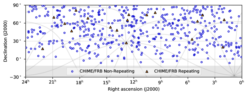
Figure 1: Sky distribution of 18 repeating sources and 474 sources that have not been observed to repeat. The gray shaded region at the bottom is outside the CHIME/FRB field of view, below declination $-11^{\circ}$. The gray lines in the background are the Galactic Plane and lines of constant Galactic longitude spaced by 30^∘. CHIME, being a transit telescope, has relatively uniform exposure in this Mercator projection of equatorial coordinates.

This paper is organized as follows. In Section 2, we describe the observing parameters, including a brief synopsis of the instrument, pipeline and overall methodologies used, as well as our sky exposure, sensitivity thresholds, and our determination of instrumental biases. In Section 3, we describe the contents of our catalog and how they were determined, including burst localizations and properties, along with relevant tables and figures. Section 4 describes our method for injecting synthetic signals into the our detection pipeline for calibrating selection biases. In Section 5, we compare parameter distributions for repeaters and apparent non-repeaters, in order to identify differences between these types of sources. In Section 6, we show parameter distributions corrected for instrumental biases and deduce cosmic distributions for many key FRB parameters, including the FRB fluence distribution. In Section 7 we discuss these results in the context of other FRB findings in the literature, and briefly describe contemporaneous analyses of these same data that are presented in accompanying papers. We present our conclusions in Section 8.

2 Observations

The CHIME telescope, its FRB detection instrument, and real-time pipeline have been described in detail elsewhere (see Table 1; CHIME/FRB Collaboration et al., 2018). Briefly, the telescope is located on the grounds of the Dominion Radio Astrophysical Observatory (DRAO) near Penticton, British Columbia, Canada, and consists of four 20-m $\times$ 100-m cylindrical paraboloid reflectors oriented N-S, with each cylinder axis populated by 256 equispaced dual-linear-polarization antennas sensitive in the frequency range 400–800 MHz. CHIME has no moving parts. The CHIME/FRB detector views the entire sky north of declination $-11^{\circ}$ (a configurable choice, see below) every day as it transits overhead. Sources northward of declination $+70^{\circ}$ are visible twice per day, on opposite sides of the North Celestial Pole. The 2048 antenna signals are amplified, conditioned, digitized, and split into 1024 frequency channels at 2.56-$\mu$s time resolution by the portion of CHIME’s correlator called the “F-Engine”, which uses 128 custom-built field programmable gate array (FPGA)-based “ICE” Motherboards (Bandura et al., 2016) housed in two radio frequency interference (RFI)-shielded shipping containers located under the reflectors. The signals are then sent to the “X-Engine”, which consists of 256 liquid-cooled GPU-based compute nodes located in two custom RFI-shielded shipping containers located adjacent to the reflectors. Within the X-Engine, the spatial correlation is performed and polarizations are summed, forming 1024 independent total intensity sky beams along the N-S primary beam (256 N-S $\times$ 4 E-W; Ng et al., 2017), as well as up-channelization to the 16k frequency channels at 0.983-ms time resolution used in the real-time FRB search. Formed beams are spaced evenly in $\sin\theta$ N-S from $\theta=-60^{\circ}$ to $\theta=+60^{\circ}$, where $\theta$ is the angle from zenith along the meridian. Formed beam centers are separated by 0.4^∘; the FWHM of each beam is approximately 0.5^∘ at 400 MHz and 0.25^∘ at 800 MHz, though the aspect ratio E-W versus N-S changes with declination (see Ng et al., 2017, for details).

Table 1: Key Properties of the CHIME Telescope and CHIME/FRB Instrument

Parameter	Value
Collecting area	8000 m2
Longitude	$119^{\circ}37^{\prime}$03$\farcs$00 West
Latitude	$49^{\circ}19^{\prime}13\farcs 08$ North
Altitude	547.9 m
Frequency range	400–800 MHz
Polarization	orthogonal linear
E-W FoV	2.5∘–1.3∘
N-S FoV	$\sim$120∘
Focal ratio, $f/D$	0.25
Receiver noise temperaturea	$\sim$50 K
Number of beams	1024
Synthesized Beam width (FWHM)	40′–20′
FRB search time resolution	0.983 ms
FRB search frequency resolution	24.4 kHz
Source transit duration	Equator: 10–5 min
	Dec = 45∘: 14–7 min
	North Celestial Pole: 24 hr

Notes. Reproduced from CHIME/FRB Collaboration et al. (2018) for convenience with updates to reflect the current operating configuration. Where two numbers appear, they refer to the low and high frequency edges of the band, respectively.
^a Including losses in the feeds, the full analog chain, and ground spill, although very approximate.

Each beam’s data are searched in real time for FRBs using a custom-developed triggering software pipeline consisting of four stages termed L0, L1, L2/L3 and L4 (CHIME/FRB Collaboration et al., 2018). Briefly, L0 is effectively the spatial correlation, beamforming, and up-channelization stage described above. L1 is the primary search workhorse, with initial cleaning of RFI (of either anthropogenic or solar origin), followed by a highly optimized tree-style dedispersion, spectral-weighting, and peak-search algorithm (called “bonsai”). L1 is executed on a dedicated cluster of 128 CPU-based nodes located in a third, custom-built shipping container adjacent to the telescope. L1 nodes are constantly buffering intensity data which can be saved upon detection of a candidate FRB event. L2/L3 combines results from all beams and groups detections to identify likely unique events, as well as further reject RFI, identify known sources, and verify a source’s extragalactic nature via its DM combined with the NE2001 (Cordes & Lazio, 2002) and YMW16 (Yao et al., 2017) models of the maximum Milky Way DM. Metadata headers (containing detection beam locations, initial DM, pulse width and signal strength estimates) for FRB candidates are stored in the L4 database, and raw intensity data buffered by L1 are saved to disk for offline analysis.

A significant change to the pipeline as described in CHIME/FRB Collaboration et al. (2018) was made to the event classification in L2/L3 in February 2019, where a high signal-to-noise ratio (SNR) classification bypass was added in response to a number of very high SNR events being misclassified as RFI. After the change, any event with $\mathrm{SNR}>100$ bypasses automatic classification and proceeds directly to human classification.

Note that as of December 2018, the CHIME/FRB realtime pipeline also triggers the recording of raw telescope baseband from CHIME’s 1024 antennas (which is buffered in memory $\sim$34 s on the X-engine) upon detection of a bright FRB candidate. A description of the baseband portion of the CHIME/FRB instrument as well as its analysis pipeline is presented elsewhere (Michilli et al. 2021; Mckinven et al. 2021, submitted), and the analysis and results of the baseband data for the 153 events in Catalog 1 for which they were captured will be presented in a future work.

2.1 Beam model

Throughout our analysis, including when evaluating the exposure, sensitivity, and when injecting synthetic events, we rely on a model of the CHIME/FRB’s beam, including the primary beam of an individual antenna element, and the interferometric synthesized beams formed digitally in the X-engine.

The CHIME primary beam, owing to its N-S oriented cylindrical reflectors, is narrow in the E-W direction and wide in the N-S direction. The primary beam is the response of a single feed over the cylinder, modulated by reflections off the ground plane and interactions between neighbouring feeds. These interactions impart characteristic spatial and spectral features to the primary beam.

A preliminary model is used for the primary beam in the analyses presented here, constructed from an outer product of independent estimates of the E-W and N-S profiles of the beam. We term this our v0 beam model, which will be described in detail in future work. Reduced dimensionality representations of the beam are shown in Figures 2 and 3. In brief, we define the beam model in telescope coordinates $x$ and $y$, which are two Cartesian coordinate components of sky locations on the unit sphere, where the $z$-axis lies at the telescope zenith and the $y$-axis points to the horizon in the direction of local celestial North. The E-W ($x$) profile is measured by tracking Taurus A with the 26-m John A. Galt Telescope at DRAO, equipped with a CHIME feed, as the source transits across the CHIME primary beam, while correlating the 26-m signal with the signal from each of the 1024 CHIME feeds (see Berger et al., 2016). This yields a high SNR measurement of the E-W profile along the source track. Since the Galt telescope uses an equatorial mount, the polarisation angle of the source can be kept fixed with respect to its feed. The profile used for the beam model in this work is an average of multiple observations of Taurus A, translated across all declinations, and stacked over all CHIME feeds separately for each polarization and frequency.

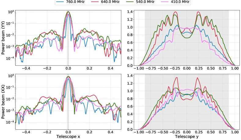
Figure 2: Slices through the primary beam model at four frequencies for each antenna polarization. Left panels show an East–West slice at the declination of Taurus A ($y=-0.46$). Right panels show a North–South slice along the meridian ($x=0$). Shaded regions represent the extent of the primary beam used to generate synthesized beams. The Cartesian coordinates $x$ and $y$ are unitless, specifying sky locations on the unit sphere, as described in the text. The beam response is shown in beam-model units where the meridian response to Cygnus A is unity at all frequencies.

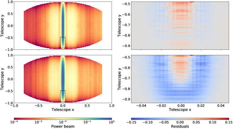
Figure 3: Frequency-averaged primary beam models and residuals from solar data comparison for each antenna polarization. The top and the bottom panels show the power response of Y and X polarizations respectively. Left panels shows the frequency median of the primary beam model for each antenna polarization. Right panel shows the frequency median of the difference between the model and measurements from transits of the Sun. The coordinate system and beam-model units are the same as in Figure 2. We take advantage of the Sun’s seasonal declination change to measure the beam over a small area (region enclosed in the dashed line in the left panel) with a single source. In the region tested, the band-averaged primary beam model is accurate to better than 10% of its peak response.

The N-S ($y$) profile provides the normalization to the peak beam response at each declination. This profile is estimated via a model that has been developed to describe the cross-talk between feeds on the focal line, referred to as the coupling response. Cross-talk can occur through several paths: e.g., radiation broadcast by a feed being directly picked up by nearby feeds (direct path) or radiation being reflected by the cylinder and reaching other feeds (1-bounce path). Each of these coupling paths introduces a delayed copy of the broadcast radiation, and a superposition of multiple such copies give rise to the coupling response. This model has a number of free parameters associated with the coupling strength for each path as a function of spectral frequency. We fit these parameters using observations of 37 bright radio point sources at different declinations. This provides an estimate of the N-S profile spanning all declinations and frequencies. By internal convention, the primary beam model is scaled such that Cygnus A (our most reliable calibrator) has unit response (1 Jy/Jy) at each spectral frequency when transiting the meridian. While we have not accounted for variability in these point sources, we have checked that consistent results are obtained using data collected six months apart.

The power responses for the two antenna polarization are averaged, meaning our beam model applies best to unpolarized sources. While FRBs are typically strongly polarized, they also typically have significant Faraday rotation which rotates the polarization angle several times over the band. As such, we expect the unpolarized beam response to be reasonably applicable when averaged over the band.

To validate this primary beam model, we use CHIME’s intensity mapping data stream to observe the Sun, which allows a range of declinations to be measured with a single source. We employ baselines shorter than 10 m while beamforming to avoid resolving out the Sun. The primary beam measurements were carried out over 2019-20, which is a known period of solar minimum. Over this span, the daily flux variability of the Sun is recorded to be $\leq$ 10% in the CHIME frequency band (Wulf et al. in prep). The comparisons are shown in Figure 3. In the region probed, we find 10% agreement between the measurements and our model for the primary beam. The low declination of the Sun compared to the CHIME latitude means we probe relatively low elevations, where the beam model is constrained by few point-source observations. As such, we consider this comparison to be the most pessimistic case for the beam model performance.

The response of the FFT synthesized beams is precisely known as they are synthesized digitally (Ng et al., 2017). We have measured the antenna-to-antenna phase variations from either calibration errors or the primary beams to be at or below the 0.01 radian level. Phase variations at this level have been shown to be negligible (Masui et al., 2019). Antenna-to-antenna amplitude variations are dominated by variations in the primary beam and exist at the 10% level. These are expected to induce percent-level perturbations to the synthesized beam. Observations of bright sources such as Cygnus A and Taurus A using the CHIME/FRB backend have been used to evaluate the composite beam model, and in particular the FFT synthesized beams since the primary beam is well characterized at these declinations. These observations match expectations at the few percent level, implying our overall uncertainty is dominated by the uncertainty in the antenna-mean primary beam.

2.2 Sky exposure

CHIME is a N-S-oriented transit telescope with cylindrical reflectors that yield a long $\sim$120^∘ N-S primary beam on the sky. The telescope operates nominally 24 hours per day. As such, CHIME/FRB’s exposure to the sky is effectively uniform in right ascension, but not in declination. Additionally, during the survey period, CHIME was not fully operational 100% of the time; there were occasional shut-offs for maintenance or software upgrades, or for unexpected occurrences like sudden power outages. Even when operational, the nature of CHIME’s infrastructure means portions may be offline. For example, a temporarily non-functional GPU node in the X-Engine results a portion of the bandwidth (1 part in 256, or 64 out of 16384 channels) being unavailable. A temporarily non-functional CPU node in the FRB cluster results in eight sky beams not being processed. To quantify the exposure and sensitivity of the telescope to FRBs, these effects must be accounted for. Metrics of all computing systems relevant to CHIME/FRB are recorded for this purpose. Metrics for the L1 nodes are recorded whenever an event (astrophysical or RFI) is detected by the real-time pipeline. Maximum temporal separation between events, and thus L1 metrics, when the real-time pipeline is functioning nominally, is of the order of a few minutes. Monitoring of the L2/L3 and L4 stages was manual with the system being checked every few hours. The exposure on the sky for each detected FRB presented here can thus be determined, as can the exposure for any position on the sky.

For the purpose of computing exposure, we consider a sky location as being detectable if it is within the FWHM region of a synthesized beam at 600 MHz and the CPU node designated for processing data for that beam is operational. We evaluate the exposure for daily transits of all sky locations with declination $\delta>-11^{\circ}$ by querying the recorded system metrics. We exclude transits observed in the pre-commissioning period (2018 July 25 to 2018 August 27) as the telescope was operating with a different beam configuration, resulting in the sensitivity to a given sky location being significantly different than that for the current configuration. Additionally, we excise transits during which the system was not operating at nominal sensitivity. System sensitivity variations arise due to changes in gain calibration and RFI environment and are characterized by analyzing distributions of SNR values for CHIME/FRB detections of Galactic radio pulsars, as described in detail by Josephy et al. (2019) and Fonseca et al. (2020). A transit is excised if it occurs on a sidereal day for which the RMS noise derived from pulsar detections exceeds the mean RMS noise in the period used for the exposure calculation by more than 1$\sigma$. On average, 7% of all transits were excised for each sky location. This is lower than the expected excision fraction for a one-sided 1$\sigma$ cut (16%) as the distribution of daily RMS noise values is not perfectly Gaussian. 23 FRB events from excised periods are not included in population distributions and analyses, as their selection function and rate statistics cannot be well-characterized.

An all-sky map of the total exposure is shown in Figure 4 with the circumpolar sky locations ($\delta>70^{\circ}$) having the two transits, upper and lower, plotted separately. We do not combine the exposure for both transits as the primary and synthesized beam response varies significantly between the two. The aforementioned sky map is then used to compute the exposure for all detected FRBs. For each source, we calculate the weighted average and standard deviation of the exposure over a uniform grid of positions within its 90% confidence localization region with the weights equal to the sky-position probability maps (see Section 3.2). The exposures for all sources with the corresponding uncertainties are provided in Catalog 1 and shown in Figure 5.

The uncertainties in the exposure calculation are due to corresponding source declination uncertainties as synthesized beam widths vary significantly with declination. Therefore, we do not report any uncertainties on the exposures for FRBs that have been localized with sub-arcsecond precision, FRB 20121102A and FRB 20180916B. (Chatterjee et al., 2017; Marcote et al., 2020). We note that some sources have exposures lower than the average value for their declination range (see Figure 5). This is due to a significant fraction of their positional uncertainty region being located between the FWHM regions of two synthesized beams (see details of localization in Section 3.2).

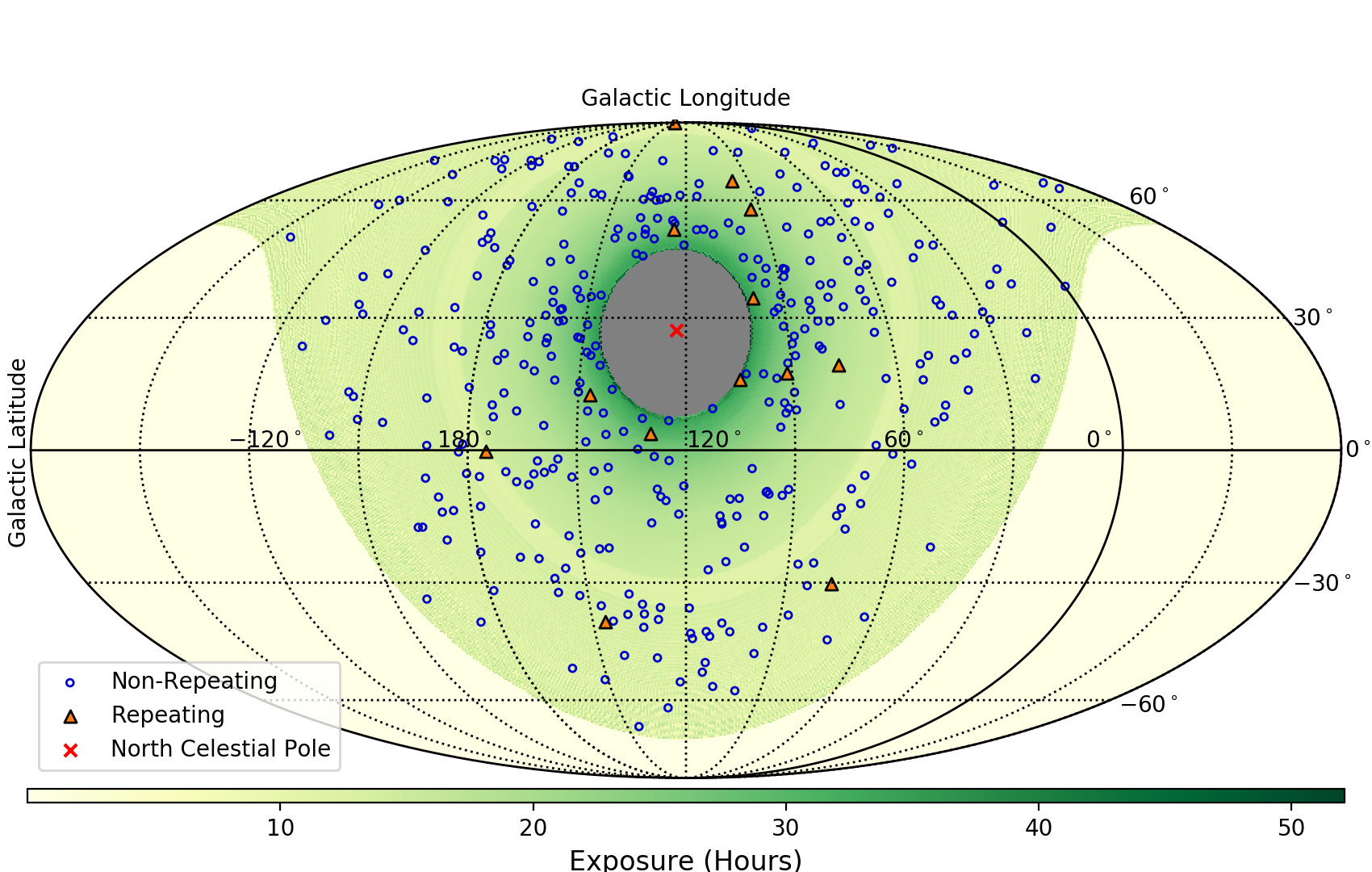
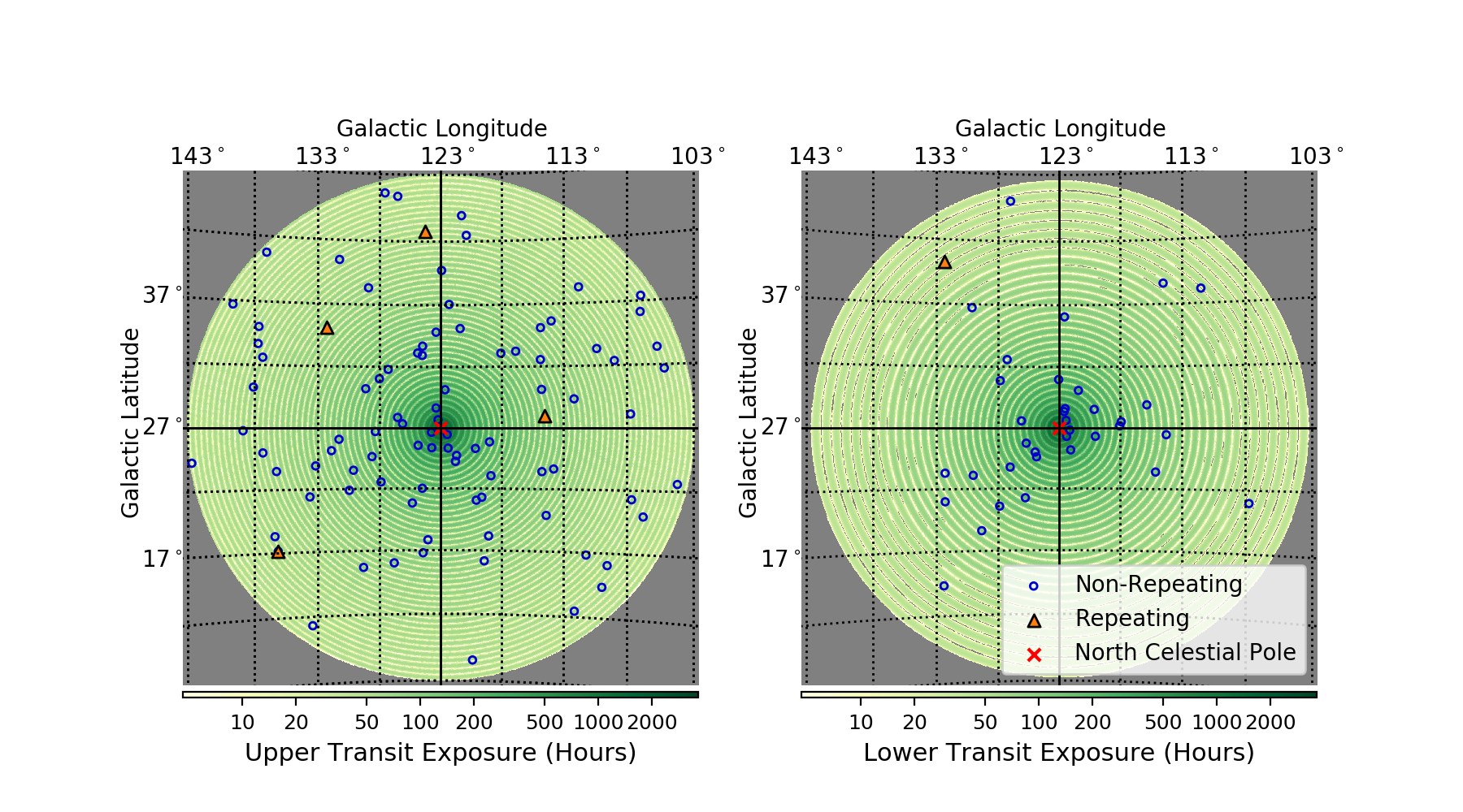
Figure 4: Sky maps in Galactic coordinates with locations of all repeating and apparent non-repeating FRB sources presented in this work overlaid on the total exposure of the CHIME/FRB system in the period from 2018 August 28 to 2019 July 1. The top panel shows sky locations that transit across the primary beam of the telescope once per day ($\delta<70^{\circ}$) while the bottom panels show upper and lower transit exposures for locations which transit across the primary beam of the telescope twice per day ($\delta>70^{\circ}$). Maps in the bottom panel are centered on the North Celestial Pole and have a logarithmic color scale. Despite comparable exposure for the two transits, there are fewer FRB detections in the lower transit due to reduced sensitivity of the primary beam as compared to the upper transit. The concentric circular patterns arise due to regions between synthesized beams having zero exposure.

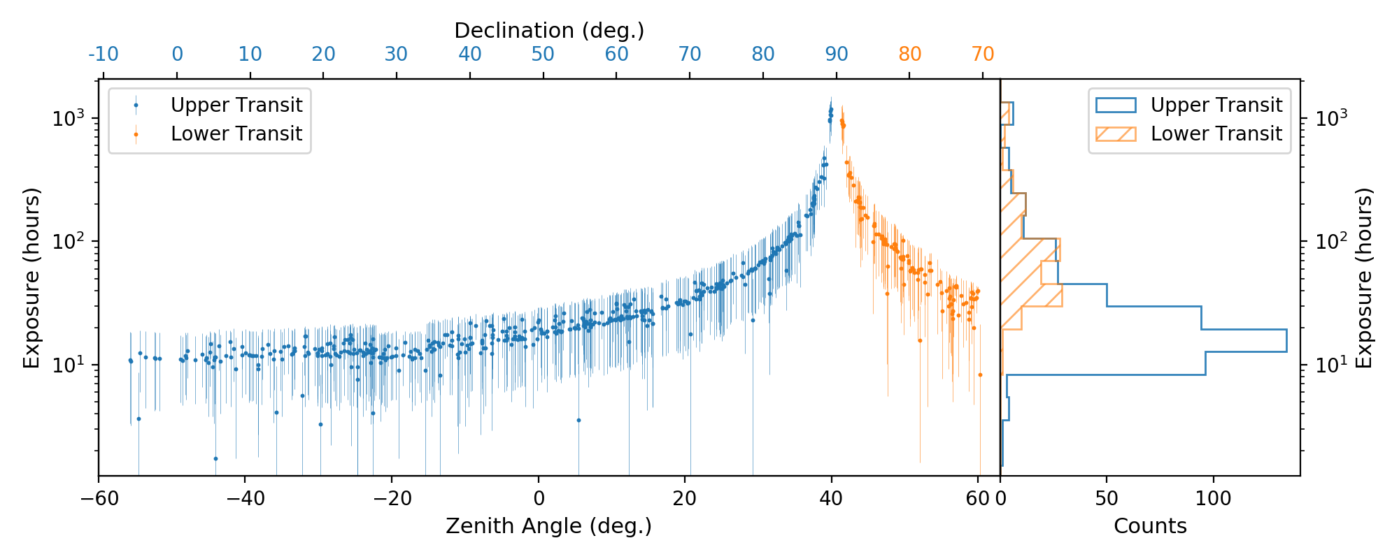
Figure 5: CHIME/FRB’s exposure for each of the sources presented in this work for upper and lower transits (if observable) plotted as a function of declination ($\delta$) and zenith angle. Errors on the exposure are due to uncertainties in source declinations (see Section 2.2). The reduced mean exposure for sources with declinations between $27^{\circ}$ and $34^{\circ}$ is due to a time-limited failure of one of the four CPU nodes (see Section 2) designated to process data for this declination range. A histogram of estimated exposure times for FRBs detected in the upper and lower transits are plotted in the right panel.

2.3 Sensitivity threshold

Exposure on the sky is distinct from sensitivity—two beams on the sky that have equal exposure may not be equally sensitive. Using recorded system metrics along with knowledge of the shapes of the primary beam and the formed beams, we have determined for each detected FRB in our catalog a sensitivity threshold for detection of FRBs.

We follow the fluence threshold methods detailed by Josephy et al. (2019) and CHIME/FRB Collaboration et al. (2019a). To estimate a sensitivity threshold across the quoted exposure, we account for three sources of sensitivity variation by generating a large number of detection scenarios in a Monte Carlo simulation. Day-to-day variation is captured with detections of known pulsars; variation as the source transits through the formed beams is computed using the beam model; and spectral sensitivity variation is estimated by combining simulated spectral profiles with the bandpass, which is obtained for each burst during the fluence measurement process, where steady-source transits provide a mapping between beamformer units and Janskys. Josephy et al. (2019) and CHIME/FRB Collaboration et al. (2019a) used Gaussian profiles for the simulated spectra and drew the defining parameters uniformly around the fitted parameters of the reference burst. In this work, we sample spectral parameters according to a Gaussian kernel density estimation of the fitted parameters from all catalog bursts. After assigning a date, position along transit, and spectrum, each simulated detection scenario leads to a sensitivity scale factor, relative to the observing conditions of the reference burst. The scale factors are then applied to the fluence threshold inferred from the measured fluence and detection SNR, resulting in a distribution of fluence thresholds. We then associate a completeness confidence interval to the corresponding percentile of the distribution. Completeness at the 95% confidence interval is reported in Catalog 1 for each source. For sources with $\delta>70^{\circ}$, we simulate fluence threshold distributions for the upper and lower transit separately. The median 95% completeness across all bursts is approximately 5 Jy ms.

3 CHIME/FRB Catalog 1

In this section, we present Catalog 1, including for each event, the event name, arrival time, sky location, DM, pulse width, scattering time, spectral parameters, and various measures of signal strength. In Table LABEL:ta:catalog, we provide a description of each field from the Catalog. The Catalog itself is available in machine readable format accompanying the online version of this article. It contains entries for each event or, in the case of complex-morphology bursts, each subcomponent of the event. A short excerpt from the Catalog can be found in Appendix E.

During the period considered for Catalog 1, there were 28 occurrences where a trigger from the real-time system fit all criteria for an FRB but, due to a malfunction of the system, intensity data were not saved. There is no way to determine whether these events would have been classified as true FRBs upon human inspection.

Next, we discuss how we determine the values for each catalog field.

Notes. The data for Catalog 1 in machine-readable format can be found accompanying the online version of this article as well as via the CHIME/FRB Public Webpage at https://www.chime-frb.ca/catalog. A small excerpt can be found in Appendix E.

All statistically significant fitburst parameters (i.e., with parameter value $v$ and uncertainty $\sigma$ such that $v/\sigma>3$) have their best-fit value and $1\sigma$ uncertainty reported; for marginal estimates, we report the $2\sigma$ upper limit obtained from fitburst.

Table 2: Description of CHIME/FRB Catalog 1 Data Fields

Column Number	Unit	Column Name	Description
0	…	tns_name	TNS name
1	…	previous_name	Previous name (if applicable)
2	…	repeater_name	Associated repeater name (if applicable)
3	degrees	ra	Right ascension (J2000)
4	degrees	ra_err	Right ascension error (see Section 3.2)
5	…	ra_notes	Notes on right ascension
6	degrees	dec	Declination (J2000)
7	degrees	dec_err	Declination error (see Section 3.2)
8	…	dec_notes	Notes on declination
9	degrees	gl	Galactic longitude
10	degrees	gb	Galactic latitude
11	hour	exp_up	Exposure for upper transit of the source
12	hour	exp_up_err	Exposure error for upper transit of the source
13	…	exp_up_notes	Notes on exposure for upper transit of the source
14	hour	exp_low	Exposure for lower transit of the source
15	hour	exp_low_err	Exposure error for lower transit of the source
16	…	exp_low_notes	Notes on exposure for lower transit of the source
17	…	bonsai_snr	Detection SNR
18	pc cm-3	bonsai_dm	Detection DM
19	Jy ms	low_ft_68	Lower limit fluence threshold (68$\%$ confidence)
20	Jy ms	up_ft_68	Upper limit fluence threshold (68$\%$ confidence)
21	Jy ms	low_ft_95	Lower limit fluence threshold (95$\%$ confidence)
22	Jy ms	up_ft_95	Upper limit fluence threshold (95$\%$ confidence)
23	…	snr_fitb	SNR determined using the fitting algorithm fitburst
24	pc cm-3	dm_fitb	DM determined using the fitting algorithm fitbursta
25	pc cm-3	dm_fitb_err	DM error determined using the fitting algorithm fitbursta
26	pc cm-3	dm_exc_ne2001	DM excess between DM determined by fitburst and NE2001 assuming the best-fit sky position of the source
27	pc cm-3	dm_exc_ymw16	DM excess between DM determined by fitburst and YMW16 assuming the best-fit sky position of the source
28	s	bc_width	Boxcar width of the pulse
29	s	scat_time	Scattering time at 600 MHza
30	s	scat_time_err	Scattering time errora
31	Jy	flux	Peak flux of the band-average profile (lower limit)
32	Jy	flux_err	Flux error
33	…	flux_notes	Notes on the burst flux
34	Jy ms	fluence	Fluence (lower limit)
35	Jy ms	fluence_err	Fluence error
36	…	fluence_notes	Notes on the burst fluence
37	…	sub_num	Sub-burst number (if applicable). If the FRB has only one burst, then the sub-burst number is 0. Sub-bursts listed in chronological order.
38	MJD	mjd_400	Time of arrival with reference to 400.1953125 MHz for the specific sub-burst.
39	MJD	mjd_400_err	Time of arrival error with reference to 400.1953125 MHz for the specific sub-burst.
40	MJD	mjd_inf	Time of arrival with reference to infinite frequency for the specific sub-burst.
41	MJD	mjd_inf_err	Time of arrival error with reference to infinite frequency for the specific sub-burst.
42	s	width_fitb	Width of sub-burst using fitburst
43	s	width_fitb_err	Width error of sub-burst using fitburst
44	…	sp_idx	Spectral index for the sub-burst
45	…	sp_idx_err	Spectral index error for the sub-burst
46	…	sp_run	Spectral running for the sub-burst
47	…	sp_run_err	Spectral running error for the sub-burst
48	MHz	high_freq	Highest frequency band of detection for the sub-burst at FWTM
49	MHz	low_freq	Lowest frequency band of detection for the sub-burst at FWTM
50	MHz	peak_freq	Peak frequency for the sub-burst
51	…	chi_sq	$\chi^{2}$ from fitburst
52	…	dof	Number of degrees of freedom in fitburst
53	…	flag_frac	Fraction of spectral channels flagged in fitburst
54	…	excluded_flag	Flag for events excluded from parameter inference due to non-nominal telescope operation (1 = excluded, 0 = included).

3.1 Event naming: transient name server

Each of our detected FRBs has been assigned a name provided by the Transient Name Server (TNS), the official International Astronomical Union (IAU) mechanism for reporting new astronomical transients. TNS names have format FRB YYYYMMDDx where YYYY is a 4-digit year, MM is a 2-digit month code, DD is a 2-digit day (all in UTC), and x is a string of 1 to 3 Latin letters, beginning with “A” for the first source reported to the TNS for the relevant UTC day, “Z” for the 26th, and in lowercase letters after this i.e. “aa” for the 27th, and so forth, up to and including “zzz”, for a total of 18278 possible unique FRBs reported on a given UTC day. The TNS functions as more than a name server, and in fact hosts basic data for all submitted FRBs. For Catalog 1 the hosted data are derived from the real-time CHIME/FRB detection pipeline. Chief among the hosted data are the DM, SNR, dispersion-corrected arrival time at $400~{}\text{MHz}$, and sky-position estimates with localization contours that can be downloaded in a machine-readable format. For previously published CHIME/FRB-detected events that are also in Catalog 1, we provide the previously published name (that followed an ad hoc and now outdated naming scheme) in the Catalog as well for reference, but we recommend henceforth referring exclusively to the TNS name. To aid the community in acquiring TNS names for their FRBs (both those already and yet-to-be detected), we provide in Appendix A instructions for doing so.

3.2 Event localization

We provide sky localizations for each of our events, determined via the header metadata determined in real-time by L1 and stored in L4. These localizations are presented in Catalog 1 as their central coordinates and approximate uncertainties, with actual localization error regions presented as plots in Figure 6.

We follow the same localization method detailed in CHIME/FRB Collaboration et al. (2019a). Ratios among per-beam SNR values are fit using least squares to beam model predictions for a grid of model sky locations and model intrinsic spectra. The mapping between $\Delta\chi^{2}$ and confidence interval is constructed from an ensemble of pulsar events identified by the real-time system, such that true positions fall within contours of a given confidence interval the appropriate fraction of the time. While this uncertainty treatment is most appropriate for pulsar-like spectra, we note that the true positions of the two localized repeaters (including 19 bursts from FRB20180916B observed over a range of hour angles), both emitting band-limited and morphologically complex bursts, are contained in the uncertainty regions of their respective CHIME/FRB SNR-based localizations. In the E-W direction, the grid of model locations is chosen to contain the main lobe of the primary beam. This span includes the first-order side lobes of the formed beams, which leads to the disjointed uncertainty regions seen in Figure 6. Where tabulated, we report the extent of the 68% confidence interval closest to the beam with the strongest detection. The disjointed contours, which include the near side lobes, can be found on the TNS for a variety of common confidence intervals.

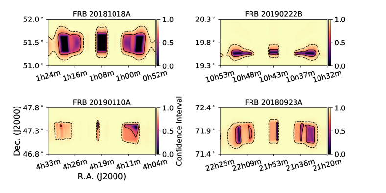
Figure 6: Example localization confidence interval plots for four different detection patterns. Clockwise from top left are: single beam, two beams N-S, two beams E-W, and four beams in a square. In each example, the frame spans 5^∘ in Right Ascension (scaled by cos(Dec.)), 1^∘ in Declination, and is centered at the beam with the strongest detection. Localization is performed as a grid-search $\chi^{2}$ minimization, where confidence intervals are obtained from contours of constant $\Delta\chi^{2}$. The color scale encodes these intervals, such that the area enclosed by a given color defines the corresponding confidence interval. The 68% and 95% intervals are shown with solid and dashed contours, respectively. Note that the common three-region pattern reflects the chromatically smeared side lobes of the formed beams. Panels for all catalog bursts can be found at https://www.canfar.net/storage/list/AstroDataCitationDOI/CISTI.CANFAR/21.0007/data/localizations/plots.

3.3 Event morphologies

The initial determination of DM provided by bonsai in the L1 real-time detection pipeline is only approximate due to the limited resolution with which it is reported (see CHIME/FRB Collaboration et al., 2018). For this reason, we used the called-back, total-intensity data saved from our L1 buffers to determine an improved DM via maximization of the SNR of the burst using offline algorithms that also provide a determination of burst time of arrival ($t_{\rm arr}$) prior to downstream model fitting. However, even the SNR optimizing DM can be significantly biased due to chromatic pulse broadening (DM-smearing and scattering) or chromatic complex burst morphology.

The SNR-optimized DM and $t_{\rm arr}$ estimates were then provided as initial guesses to a least-squares fitting routine, fitburst, that directly models the two-dimensional dynamic spectra in terms of fundamental burst parameters. For a single burst, the parameters modeled by fitburst are: DM; $t_{\rm arr}$, signal amplitude ($A$), temporal width ($w$), power-law spectral index ($\gamma$) and “running” of the spectral index ($r$), and a timescale for multi-path scattering of the FRB signal ($\tau$; e.g., McKinnon, 2014). The composite model for a scattered, single-component dynamic spectrum with label $i$ ($S_{i}$) is defined as $S_{i}=A_{i}\times F_{i}\times T_{i}$, where: $A_{i}$ is the overall amplitude of the $i^{\rm th}$ burst component; $F_{i}\equiv F_{i}(\gamma_{i},r_{i})$ is a term that defines the time-independent spectral energy distribution as a function of frequency ($f$), relative to an arbitrary reference value ($f_{0}$):

$$F_{i}(\gamma_{i},r_{i})=(f/f_{0})^{-\gamma_{i}+r_{i}\ln{(f/f_{0})}};$$ (1)

and $T_{i}\equiv T_{i}({\rm DM},t_{{\rm arr},i},w_{i},\tau)$ is a term that models the temporal shape of the burst:

$$T_{i}({\rm DM},t_{{\rm arr},i},w_{i},\tau)=\frac{1}{2\tau}\exp{\bigg{(}\frac{w_{i}^{2}}{2\tau^{2}}\bigg{)}}\exp{\bigg{[}-\frac{(t({\rm DM})-t_{{\rm arr},i})}{\tau}\bigg{]}}\bigg{\{}1+{\rm erf}\bigg{[}\frac{t({\rm DM})-(t_{{\rm arr},i}+w_{i}^{2}/\tau)}{w_{i}\sqrt{2}}\bigg{]}\bigg{\}}.$$ (2)

The form of $T_{i}$ shown in Equation 2 is taken directly from McKinnon (2014), which represents the convolution between a Gaussian profile and a time-dependent exponential function, the latter function with characteristic decay timescale $\tau$ and truncated at $t=t_{{\rm arr},i}$ by a Heaviside function.

Using the above definitions, we modeled a multi-component burst as $S=\sum_{i}^{n}S_{i}=\sum_{i}^{n}A_{i}\times F_{i}\times T_{i}$, where $n$ is the number of distinct sub-bursts in the observed dynamic spectrum. We set $f_{0}=$ 400.1953125 MHz which is the center of our lowest frequency channel, in order to be consistent with L1 configuration settings. Both DM and $\tau$ are considered to be “global” parameters, such that all sub-burst components are assumed to possess the same dispersion and scattering properties, while all parameters with subscript $i$ indicate component-specific parameters. Moreover, we assumed that $t({\rm DM})=k{\rm DM}(f^{-2}-f_{0}^{-2})$, where $k=(2.41\times 10^{-4})^{-1}$ s pc^-1 cm³ MHz² (consistent with physical expectations for dispersion in a cold plasma), and that $\tau\propto f^{-4}$ (Lang, 1971; Lorimer, D. R. and Kramer, M., 2005), where we use 600 MHz as the scattering reference frequency.

For a given CHIME/FRB event with $n$ sub-bursts, we fitted for (2 + 5$n$) parameters with fitburst through $\chi^{2}$ minimization between the $n$-component model and full-resolution L1 data. We accounted for intra-channel dispersion smearing during each fit iteration by evaluating the model spectrum $S$ at 8 and 4 times the data resolution in time and frequency, respectively, and subsequently downsampling to the data resolution. Moreover, all CHIME/FRB raw data were processed for automatic excision of narrowband RFI and noise-baseline subtraction prior to model fitting, though we did not explicitly calibrate the CHIME bandpass.

We generated two models with fitburst for each CHIME/FRB event and compared best-fit statistics in order to determine the significance of multi-path scattering in spectra. One model was generated while simultaneously fitting for all parameters discussed above, including $\tau$; for these models, $w$ is interpreted as the width of the intrinsic, pre-scattered burst component. A second model was generated assuming zero scattering, in which case the function $T({\rm DM},t_{{\rm arr},i},w_{i},\tau=0)$ in Equation 2 is replaced with a Gaussian function of standard deviation $w_{i}$ that reflects the full temporal width of profile component $i$. The $\chi^{2}$ values for both models were then compared through an F-test for model selection, and a $p$-value threshold of 0.1% was used to declare the significance of $\tau$. In cases where scattering is not significant, we quote an upper limit on $\tau$ of $2\times w$. In cases where the fit of the width-scattering model is highly degenerate (i.e., when the covariance matrix after least-squares optimization is singular), we default to the no-scattering model as the superior description. Simulations have shown that CHIME/FRB total intensity data can be used to robustly measure values of $w$ and $\tau$ larger than 100 $\mu$s only; for cases where the fitted value is smaller than this we quote 100 $\mu$s as an upper limit.

The above procedure was performed automatically on each burst. However, manual intervention was frequently required to adjust the parameter initial guesses when the least-squares optimizer failed to converge on a satifactory result. In addition, for bursts visually determined to have a complex morphology, the value of $n$ was chosen manually.

The fitting procedure described here has a number of limitations, including that the model may be an imperfect description of the intrinsic burst morphologies; inhomogeneities in the spectral frequency response from the beam and non-uniform noise; limited ability of the least-squares optimizer to converge on a global best fit and represent uncertainties; and the reliance on human judgement to assess adequate convergence and determine component count for complex bursts. These limitations are discussed in detail in Appendix B, where we also describe metrics that can be used to assess the quality of the fits on a burst-by-burst basis. Improvements to this procedure, including the use of Markov Chain Monte Carlo (MCMC) techniques and an automatic determination of $n$, are ongoing and will be the subject of future CHIME/FRB catalogs.

Best-fit parameters from the above modeling procedure are provided in Catalog 1. Tabulated uncertainties denote the 68% confidence level unless otherwise specified. Upper limits are denoted with a “$<$” symbol and represent 95% confidence upper limits unless otherwise specified.

We also derive a full-width-tenth-maximum (FWTM) emission bandwidth from the model fits, capped at the top and bottom of the CHIME band. We measure a total burst duration in the dedispersed and frequency-averaged time series. Each time series is convolved with boxcar kernels with durations equal to integer multiples of the sampling time up to 128 samples (although the search range was manually tweaked in a few cases) and normalized by the square-root of their respective widths. The burst duration is defined as the width of the boxcar that results in the highest peak SNR after convolution. FRBs 20181019A, 20181104C, 20181222E, 20181224E, 20181226B, 20190131D, 20190213B and 20190411C have two distinct peaks in their time series (without a “bridge” in emission) and for those FRBs we report two burst durations.

Time series depicting each burst, along with its dynamic spectrum (or “waterfall plot”) and spectrum, with all three dedispersed to the optimal fitburst-determined DM, are provided in Figures 7 and 8. In these plots, we have overlaid the frequency-averaged and time-averaged fitted models on the time series and spectra, respectively. We also show the burst duration and emission bandwidth FWTM. For all FRBs, we show 128 frequency subbands. Time windows are multiples of 12.5 ms, based on the FRBs’ width and scattering time scale.

For better visualization, we mask subbands with variance $>3\times$ the mean variance, and subbands with time-averaged values $<$ Q1$-1.5\times$IQR or $>$ Q3$+1.5\times$IQR, where Q1 and Q3 are the first and third quartiles, respectively, and IQR is the interquartile range. The color scales are capped to the 1^st and 99^th percentiles.

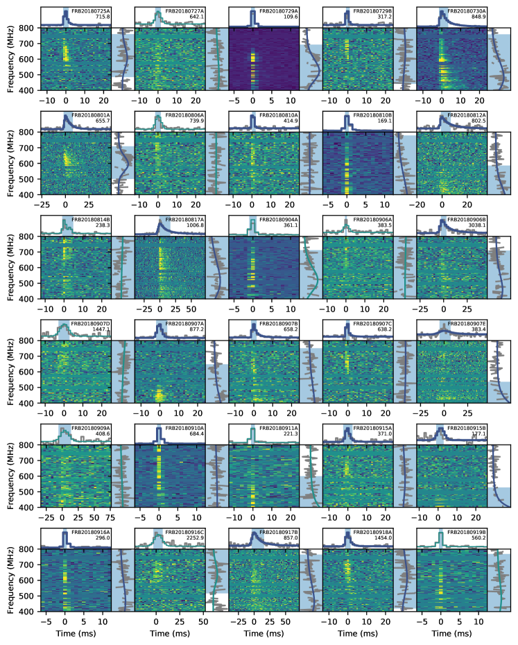
Figure 7: Dynamic spectra (“waterfall plots”), frequency-averaged time series and time-averaged spectra for all one-off FRBs in the Catalog, ordered by time. The TNS name and best-fit DM in units of pc cm^-3 are in the top right corner of each panel. Model fits are overlaid on the time series and spectra, in green (thin lines) if scattering was not significant and in blue (thick lines) if scattering was significant. The blue shaded regions in the time series and spectra indicate the burst durations and emission bandwidths FWTM, respectively. Bursts indicated with an asterisk are published repeaters, for which only one burst was detected before the Catalog cut-off date. Panels for all catalog one-off bursts can be found at https://www.canfar.net/storage/list/AstroDataCitationDOI/CISTI.CANFAR/21.0007/data/additional_figures/waterfalls.

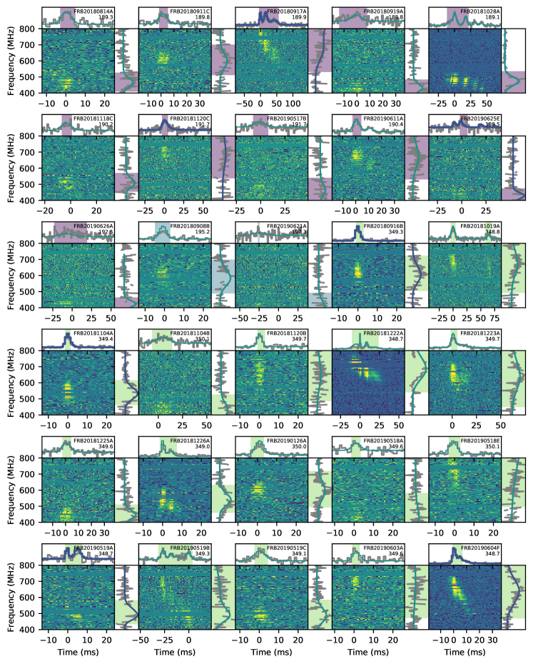
Figure 8: Same as Figure 7, but for all sources exhibiting more than one burst in this Catalog. Sources are ordered by their first detections, and bursts from any one source are ordered by time of detection. Differently colored shaded regions are used for different repeater sources. Panels for all catalog repeating bursts can be found at https://www.canfar.net/storage/list/AstroDataCitationDOI/CISTI.CANFAR/21.0007/data/additional_figures/waterfalls.

3.4 Event signal strength

To characterize signal strength for each event, we provide the SNR of the initial real-time pipeline detection, along with a fluence and flux determined in offline analyses.

In Catalog 1, our ability to determine burst fluences is limited by the uncertainty of our burst localization combined with CHIME’s complex and rapidly varying beam pattern. In particular, the spectral structure of the beam pattern and overall beam response can change significantly over the extent of the header localization region obtained for each burst, making it difficult to reliably correct fluence measurements for beam attenuation. Localization uncertainty, and to a lesser extent beam model uncertainty, introduces an unknown primary beam response that is a strong function of a bursts uncertain hour angle (see Figure 6). As such, we assume that each burst was detected along the meridian of the primary beam (at the peak sensitivity of the burst declination arc). Thus, our fluence measurements are biased low, as bursts off-meridian will experience beam attenuation that we are not accounting for. Note that the errors on the fluences, discussed below, do not quantify this bias—the measurements we provide are most appropriately interpreted as lower limits, with an uncertainty on the limiting value. A detailed description of the automated fluence calibration pipeline, including an explanation of current limitations, will be provided elsewhere. Here, we summarize the procedure, which is similar to that used in previous CHIME/FRB papers (CHIME/FRB Collaboration et al., 2019b, c; Josephy et al., 2019; CHIME/FRB Collaboration et al., 2019a; Fonseca et al., 2020).

Transit observations of steady sources with known spectral properties are used to sample the conversion from CHIME/FRB beamformer units to Janskys as a function of frequency across the primary beam. We pair each burst with the calibration spectrum of the nearest steady source transit, closest first in declination, then in time. We assume N-S beam symmetry, so that sources on both sides of zenith can be used for each event. By applying the calibration spectrum to the total-intensity data for each burst, we derive a dynamic spectrum in physical units roughly corrected for N-S primary beam variations. The fluence is then derived by integrating the burst extent in the band-averaged time series, while the peak flux is the maximum value within the burst extent (at 0.98304 ms resolution).

The error due to differences in the primary beam between the calibrator and the assumed FRB location along the meridian is estimated by using steady sources from a single day to calibrate each other and measuring the average fractional error compared to known flux values. This contributes a relative error on the order of 20% to the flux measurements. The error due to temporal variation in the calculated beamformer unit to Jansky conversion spectra is determined by measuring the RMS variation over a period of roughly two weeks surrounding the burst arrival. This also captures uncertainty due to calibrator source variability on that time scale, and contributes a relative error on the order of 13% to the flux measurements, depending on the calibrator used. These two errors are also combined with the RMS of the off-pulse in the band-averaged time series to form the overall errors presented in Catalog 1. We note again that the errors estimated here do not encapsulate the bias due to our assumption that each burst is detected along the meridian of the primary beam, which causes our fluence measurements to be biased low.

During the period from the beginning of the Catalog to February 2019, the flux calibration pipeline was still being commissioned and steady source observations were sparse. We conservatively estimate the time error for bursts detected during this time by taking the fractional RMS variation in the calibration spectrum over the entire period, yielding errors typically on the order of 26%. An additional error is included in the fluence estimates of the first 13 CHIME/FRB bursts to account for the phase-only complex gain calibration used during the pre-commissioning period when they were detected, as described in CHIME/FRB Collaboration et al. (2019b).

A total of 6 bursts were detected directly after a system restart, when we were not able to obtain steady source transits before upstream complex gain calibration was applied. Since we could not measure proper beamformer unit to Jansky scalings during these times, we do not provide fluences or fluxes for these bursts. We also note that early detected bursts previously presented in CHIME/FRB Collaboration et al. (2019b), CHIME/FRB Collaboration et al. (2019c), and Josephy et al. (2019) have been re-analyzed using the automated Catalog 1 pipeline, and their reported fluences have changed significantly due to updates in our RFI mitigation methods.

4 Synthetic signal injection

As for any astrophysical instrument, CHIME/FRB has a transfer function, introduces selection biases, and adds noise due both to the nature of the telescope and the software detection pipeline. These instrument characteristics need to be carefully characterized so that they can be accounted for in any population analysis of FRB events and their distributions, as is performed in Section 6 below. We account for these biases through careful measurements of the telescope beam, calibration, and noise properties, and by probing the selection function using Monte Carlo techniques with synthetic events injected into the CHIME/FRB software system. This strategy mimics the Monte Carlo event generator techniques used in particle physics, with the exception that real-time telescope noise and the RFI environment are incorporated by injecting the events in situ while the telescope is operating. The Monte Carlo injection system was designed to allow synthetic FRBs to be injected into the real-time pipeline with user-defined properties. Injected pulses (hereafter “injections”) are suitably flagged to ensure none are mistaken as genuine astrophysical signals. In this way, we measure instrumental biases, and using this knowledge, in Section 6 determine actual cosmic FRB property distributions.

The details of the injection system will be described elsewhere. Here we provide a brief description of the use of the injection system to quantify our instrumental and software detection pipeline biases. Figure 9 shows a schematic drawing of the injection system as it is currently set up in the full CHIME/FRB system (see also Figures 4 and 6 in CHIME/FRB Collaboration et al. 2018).

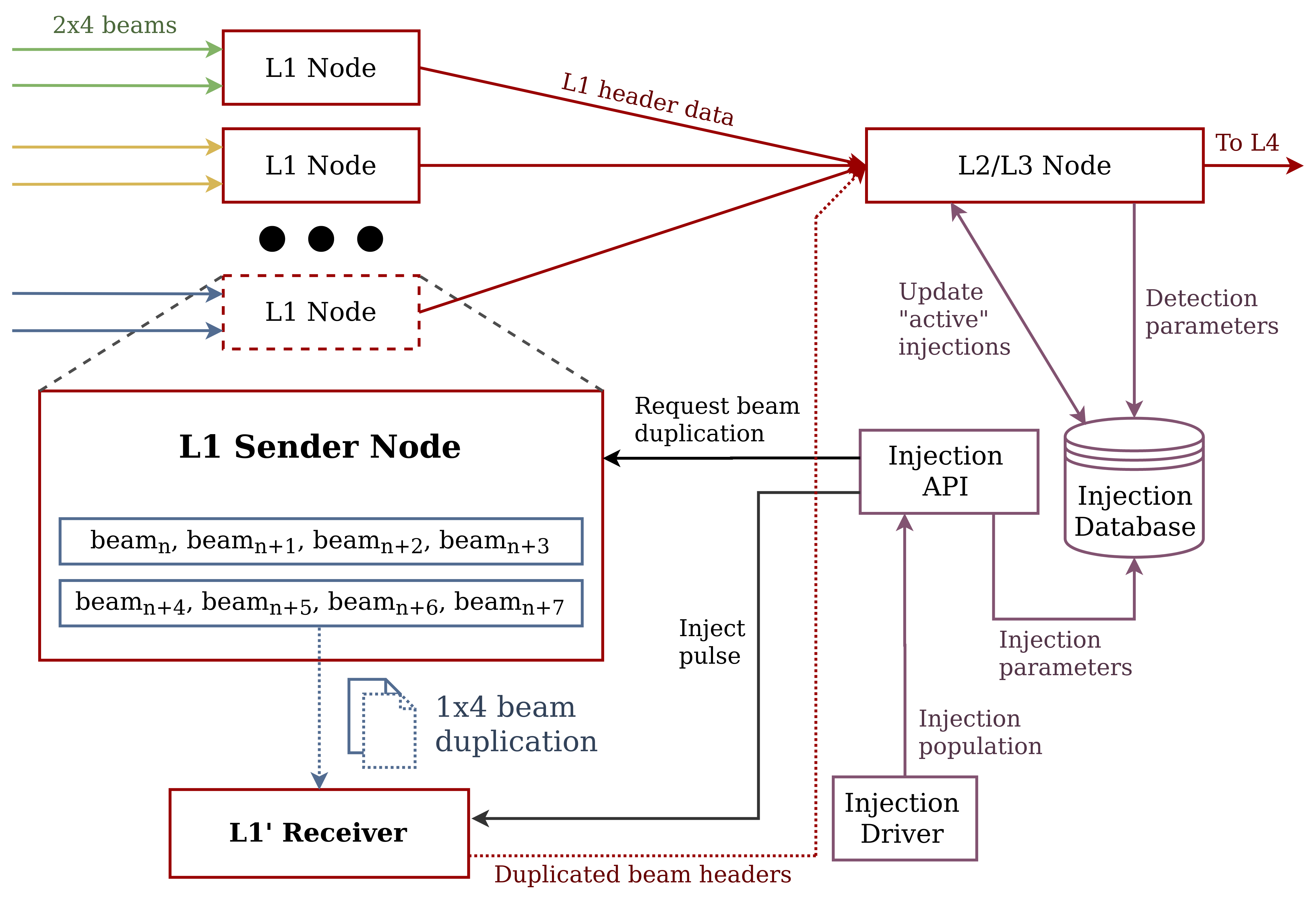
Figure 9: Schematic of the CHIME/FRB Injection System. Each L1 node handles two data streams containing full-resolution intensity data for four beams. The injection system interacts with the L1 nodes through remote procedure calls. Its capabilities are outlined in Section 4.1. The system injects a population of FRBs into the on-sky data streams of four duplicated beams at a time, and measures the events’ detection properties, storing the injection and detection parameters in a database. The green, yellow, and blue arrows indicate intensity data streamed from sets of four beams. Red boxes and arrows indicate components of the real-time pipeline and header data, respectively. Purple boxes and arrows indicate components and data flow related to the injection system. Black boxes and arrows indicate HTTP request handling interfaces and requests.

4.1 Signal generation

FRB signals are generated using the internally-developed simpulse library. simpulse generates FRBs at the CHIME/FRB frequency channel width and sampling time with an intrinsic running power-law spectrum, DM, pulse width, and scattering time. The simpulse library accounts for intrachannel dispersion smearing and other sampling effects that would occur at the correlator stage for an astrophysical signal. The injected FRB signal is multiplied with the complex spectral signature of the CHIME telescope’s primary beam and FFT synthesized beams evaluated at the chosen position in the sky.

Signals are scaled to the same absolute flux (Jy) units as the live telescope data stream. Prior to beamforming, an absolute calibration (derived from daily observations of bright continuum point-sources through CHIME’s visibility data stream) is applied to the baseband data in the X-engine. Thus, we generate our simulated signals in flux units, taking care to also apply factors introduced in the beamforming and upchannelization process.

4.1.1 Injections population

Here we describe how we generate a population of FRBs for injecting into the CHIME/FRB real-time detection pipeline using the system described in Section 4. We start by sampling locations in the sky where we will evaluate our beam model and place simulated FRBs. We randomly sample $10^{6}$ locations uniformly distributed on the celestial sphere in telescope coordinates. Of these, we discard all locations: that are below the horizon; for which the band-averaged primary beam response is less than $10^{-2}$ in beam model units (see Section 2.1); and for which the band-averaged response does not reach $10^{-3}$ in any of the 1024 synthesized beams. As such, we are not injecting bursts into the far side lobes; however, this does not incur a bias since such events are cut from the catalog for population inferences. The fraction of sky locations surviving these cuts is $f_{\rm sky}=0.0277$. Note this “forward-modeling” method of accounting for the telescope’s beam response is distinct from the simpler analyses done in other rate estimations; it is important in our case because of the complex CHIME beam.

We then draw $5\times 10^{6}$ FRBs and randomly assign them to the surviving sky locations. The properties of these FRBs are drawn from initial probability density functions $P_{\rm init}(F)$, $P_{\rm init}(\mathrm{DM})$, $P_{\rm init}(\tau)$, $P_{\rm init}(w)$, and $P_{\rm init}(\gamma,r)$ designed to both fully sample the range of observed properties and more densely sample parts of phase space populated by the catalog. The FRB properties in these distributions are uncorrelated except for $\gamma$ and $r$. These distributions are described in more detail in Section 6 and Appendix C. After drawing from the initial distributions, we perform a cut of events that have little chance of being detected based on the FRB properties, our beam model, and a conservative noise model. This left 96 942 events scheduled for injection. Due to overlapping sensitivity, true FRBs can be detected in multiple beams simultaneously. The injections system does not currently support multi-beam injections; instead, we inject a given event into the beam with the highest predicted SNR based on the noise and beam model.

4.1.2 Injection and detection

One of the 128 L1 nodes has been outfitted as a “receiver node” (L1^′) for the purposes of injections. L$1^{\prime}$ receives a stream of duplicated data for four North-South adjacent intensity beams. These data are processed using the same software as the rest of the L1 nodes. Synthetic pulses are injected into the duplicated data through an interfacing server. This server manages beam duplication, and is capable of selecting which set of four beams are being streamed to L1^′ in the live system. Careful flagging of injected events in the duplicated data streams ensures that none of the injected signals are misclassified as true astrophysical events.

The injection system injects FRB signals using user-defined parameters. The FRBs to be injected are grouped by the beams in which they are expected to have the highest SNR based on the beam model. A module known as the injection driver chooses a set of four consecutive beams at random from the 1024 CHIME/FRB intensity beams and requests the injection server to start the duplication of these four beams to the L1^′ receiver node. The injection system then waits for 300 seconds for the running estimates of the noise properties using in L1 to achieve steady-state. The injection signals prescribed for these beams are generated and injected with a minimum interval of 1 second. However, the typical interval is 2–3 seconds, the actual time required to generate and inject an FRB.

Every injection successfully injected into the data stream without software failure is noted in a database and a unique ID is generated. An “injection snatching” module in the L2/L3 pipeline is provided with a list of “active” injections that are expected in the near future along with their unique IDs, expected DM, expected arrival time, and beam number. An FRB trigger that is detected at the same time and DM (within a threshold based on the size of the bonsai DM bins) and from the same beam number is marked as an identified injection and the detection parameters are reported to the injection database tagged with the unique ID.

Of the 96 942 events scheduled for injection, we were able to inject 84 697 for an injection efficiency of $\epsilon_{\rm inj}=0.874$. Failures to inject events were due to system errors and affect an essentially random subset of injections. We injected into the predicted maximum-SNR beam during a campaign in August 2020. Of these, 39 638 events were detected and assigned a bonsai SNR.

The sensitivity of the telescope during the injections campaign in August 2020 is not perfectly representative of the sensitivity during the catalog period one to two years earlier. Based on the detection SNRs of pulsars (tabulated daily), we estimate our noise levels have improved by 6% since the beginning of the survey and 3% since midpoint of the survey period. These changes are accounted for in our population analysis and systematic error budget as described in Appendix D. Furthermore, several periods of low sensitivity or differing instrument configurations (including the pre-commissioning period over which our first 13 bursts were discovered) are not well represented by the injections campaign. These periods, and the bursts discovered therein, are thus excised from further analyses that rely on injections. Finally, numerous tweaks to the operations of the instrument have occurred over and since the observation period. These tweaks mostly served to streamline observations and to increase the instrument uptime (for which we have a separate accounting) and have caused only small changes in our completeness. However, since our observations occurred prior to the availability of the injections system, changes in our completeness over time are difficult to quantify. Such effects should be better quantified in future data releases where injections can be performed throughout the observations.

5 Comparison of Repeaters versus Apparent Non-Repeaters

This catalog represents by far the largest number of FRBs collected in a uniform manner using a single telescope and detection pipeline. This uniformity is helpful for studying FRB property distributions, as past analyses have been complicated by using FRBs from multiple surveys having very different survey parameters (e.g. Lawrence et al., 2017).

The central challenge in studying the FRB population from our data set is compensating for selection effects (e.g. it is more difficult to measure a narrow intrinsic burst width in the presence of strong scattering) and instrument-induced biases (e.g. it is more difficult to measure narrow intrinsic burst widths due to our finite time resolution) in event reconstruction. For some FRB properties (e.g., fluence, scattering), selection effects are strong and our fractional completeness varies by orders of magnitude across the range of detected values for the property. For other properties (e.g., DM), selection effects are at the factor-of-two level.

We use two strategies for dealing with these selection effects. In this section, we compare repeater burst properties to those of apparent non-repeaters, under the reasonable assumption both suffer the same selection biases, subject to minor caveats discussed below. In this way we can deduce in a direct way differences in properties between the two observational classes. However, this comparative method does not permit an absolute measurement of the characteristics of either population, for example the fluence distribution or overall sky rate. In contrast, in Section 6, we explicitly measure and compensate for selection effects using injections, but only for the total population for which we have the best statistics.

For both analyses, we perform a set of cuts on the catalog to remove events which are especially susceptible to selection effects that are challenging to quantify. These include the following:

1. Events with bonsai $\mathrm{SNR}<12$ are rejected, since below this threshold there could have been real events detected by our pipeline but subsequently classified as noise upon human inspection. During human classification, events with $\mathrm{SNR}\geq 12$ are visually unambiguous as either FRBs or RFI.

2. Events having $\mathrm{DM}<1.5\max(\mathrm{DM}_{\rm NE2001},\mathrm{DM}_{\rm YMW16})$ are rejected. This cut is more stringent than that used for classifying events as extragalactic FRBs. The purpose is to reduce unquantified incompleteness coming from misidentifying FRBs when localization errors induce an error in the estimated Galactic DM. It also reduces any dependence our results may have on the poorly understood systematic errors associated with the Galactic DM models.

3. Events detected in far side-lobes are rejected, as our primary beam is poorly understood in this regime. These far side-lobe events have visually-identified “spiky” signatures in the burst spectrum (e.g., CHIME/FRB Collaboration et al., 2020b).

These cuts eliminate 205 Catalog 1 FRBs (dominated by the SNR cut) from the following analysis.

The assumption of identical biases for non-repeaters and repeaters is certainly untrue since we reduce our trigger threshold for the directions and DMs of previously detected FRBs, to be additionally sensitive to repeat bursts. For this reason, unless specified otherwise, we compare only the first-detected repeater events for each repeating source, since that event’s trigger threshold was at the nominal value, thereby eliminating any possible disparity, and avoiding statistical complications of having multiple events per source. More subtly, the assumption of identical biases for repeaters and apparent non-repeaters, even with identical thresholds, is also likely untrue given the differences in burst widths and bandwidths shown below and described in detail by Pleunis et al. (2021, submitted) and previously reported (CHIME/FRB Collaboration et al., 2019a; Fonseca et al., 2020), coupled with the fact that selection effects are correlated (as discussed in detail in Section 6). Nevertheless, in this analysis we are only sensitive to differences in the selection-induced correlations between the two sub-populations, which, while we have not explored this effect in detail, we expect it to be small and unlikely to affect the conclusions of our comparison. Note that although we consider only Catalog 1 events with $\mathrm{SNR}\geq 12$, we have verified that all conclusions below hold when all catalog events, regardless of SNR, are included.

For all distribution comparisons, we report probabilities from both Anderson–Darling ($AD$) and Kolmogorov–Smirnov ($KS$) tests, where a $p$ -value $<0.01$ implies $>99$% confidence that the two samples are drawn from different underlying distributions.

5.1 Sky distribution comparisons

First we compare the sky distributions of repeaters and non-repeaters, specifically their right ascension and declination distributions (see Figure 10). For right ascension, we find no difference in the distributions ($p_{AD}=0.22$, $p_{KS}=0.24$), with both consistent with a uniform distribution when including bursts at all declinations. Similarly for declination, the two distributions are statistically consistent ($p_{AD}=0.55$, $p_{KS}=0.49$). Note that the declination distributions in Figure 10 are not corrected for exposure and sensitivity, but such corrections affect both repeaters and non-repeaters similarly. One caveat is that near the North Celestial Pole, our source density is high due to the long exposure (see Figure 4) which results in confusion that makes repeater identification more difficult than at lower declinations. Ignoring the Polar region only strengthens the conclusions that the declination distributions of repeaters and apparent non-repeaters are statistically consistent with arising from the same sky distribution. We note that the apparent peak in the declination distribution of non-repeating FRBs at $\sim$ 28^∘ is consistent within 2$\sigma$ with the remainder of the distribution. Separately, we have performed detailed analyses of the sky distribution of our Catalog 1 sources. Specifically, Josephy et al. (2021, submitted) search for evidence of correlation with Galactic latitude as has been previously claimed (Burke-Spolaor & Bannister, 2014; Petroff et al., 2014; Macquart & Johnston, 2015; Bhandari et al., 2018). We also report on a search for correlation with large scale structure in future work.

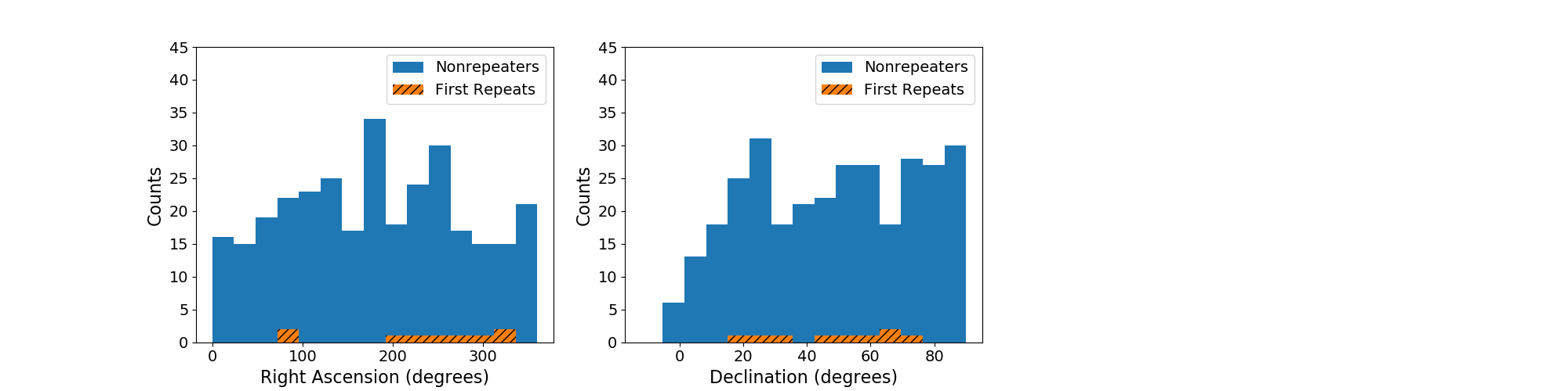
Figure 10: Observed distributions in right ascension (left) and declination (right) of apparent non-repeaters and the first-detected repeater events from Catalog 1. Note neither is corrected for exposure. In both cases, the first-detected repeat bursts and apparent non-repeater bursts are statistically consistent with having come from the same underlying distribution.

5.2 DM comparisons

Next, we consider the observed and extragalactic DMs of apparent non-repeaters and first-detected repeater events from Catalog 1, where extragalactic DM is defined as the observed DM minus the maximal line-of-sight component predicted by NE2001; see Figure 11. We find that the distributions are consistent with being drawn from the same underlying distribution for DM ($p_{AD}=0.35$, $p_{KS}=0.33$) and for extragalactic DM ($p_{AD}=0.34$, $p_{KS}=0.24$).

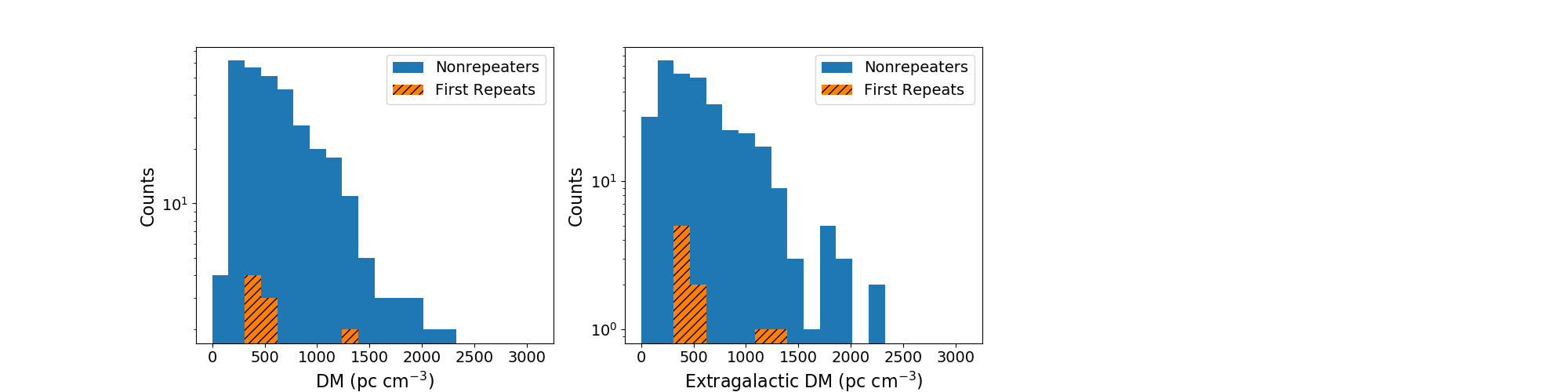
Figure 11: Observed distribution of DMs (left) and extragalactic DM (subtracting the maximal NE2001 component) of apparent non-repeaters and the first-detected repeater events from Catalog 1. In both cases, the first-detected repeat bursts and apparent non-repeater bursts are statistically consistent with having come from the same underlying distribution.

5.3 Signal strength comparisons

Next we compare direct measures of signal strength, SNR, as measured by the initial trigger SNR from our real-time FRB search code bonsai (CHIME/FRB Collaboration et al., 2018) and also by our intensity data burst code, fitburst (see Section 3.3). Note that neither of these two SNR measurements is a faithful representation of the true signal strength at the telescope aperture, because of the complex, frequency-dependent CHIME beam response. Moreover, bonsai SNR is corrupted by RFI mitigation (clipping) for very bright bursts, an effect with complex behavior in time and spectral frequency. The repeater and non-repeater samples could be differentially affected by the beam, clipping, or other effects, since the two populations have intrinsically different spectro-temporal properties (studied in detail below). Even so, the comparison is interesting since an observed difference is indicative of an intrinsic difference in the populations, even if it might be indirect through correlated observational effects. The distributions are shown in Figure 12. The repeater and apparent non-repeater distributions are consistent with being drawn from the same population for both SNR measures ($p_{AD}=0.65$, $p_{KS}=0.44$ for bonsai SNR and $p_{AD}=0.08$, $p_{KS}=0.26$ for fitburst SNR).

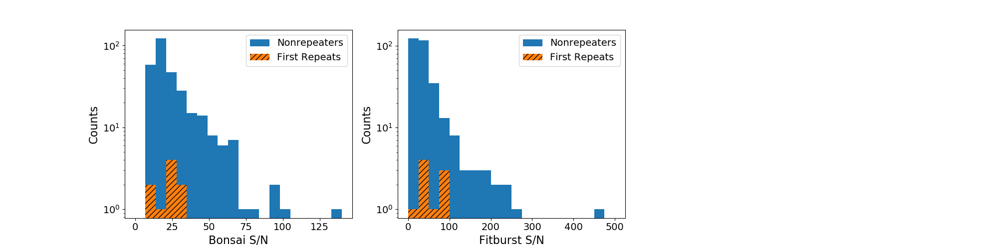
Figure 12: Distributions of bonsai (left) and fitburst (right) SNRs for apparent non-repeaters and first-detected repeater events. The repeater and apparent non-repeater distributions are consistent with being drawn from the same population for both SNR measures, although the p-values (see text) are somewhat low for the fitburst SNR comparison, with a possible relative paucity of repeater bursts at the very lowest SNRs.

We can also compare signal strength distributions using calibrated fluence and flux, noting, however, that our values have substantial uncertainties and are biased low, mainly due to the unknown location of each event within the detection beam (see Section 3.4). The distributions are shown in Figure 13. The fluence distributions are consistent with being drawn from the same underlying sample, ($p_{AD}=0.070$, $p_{KS}=0.066$), as are the flux distributions, though with lower $p$-values ($p_{AD}=0.028$, $p_{KS}=0.068$). A possible origin for this putative, slight difference is the broader widths for repeaters (see below). We note that also including Catalog 1 events with $\mathrm{SNR}\geq 12$ results in similarly low but still inconclusive $p$ -values ($p_{AD}=0.028$, $p_{KS}=0.021$ for fluence and $p_{AD}=0.040$, $p_{KS}=0.044$ for flux), so does not lend additional support to the distributions being different.

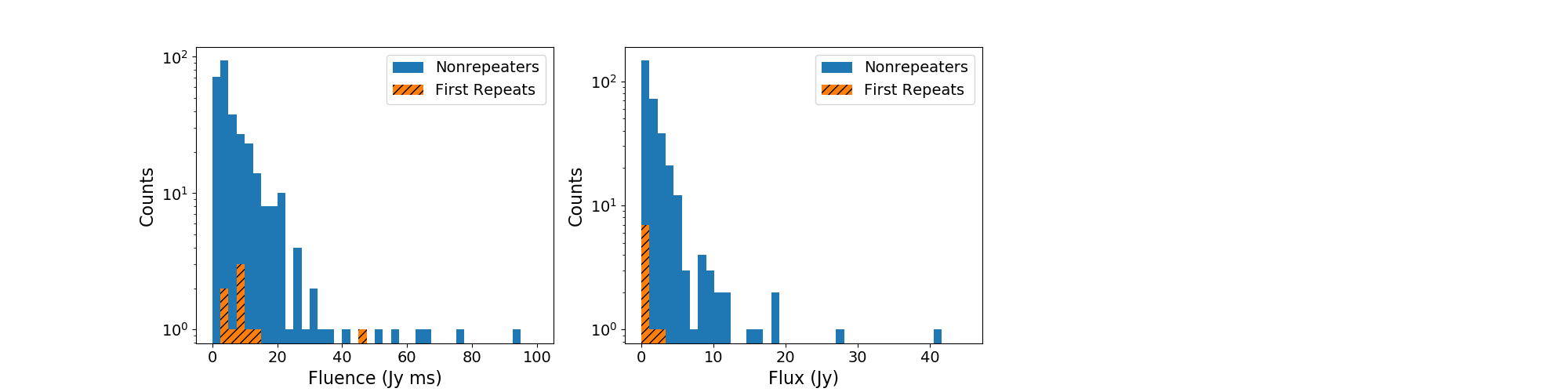
Figure 13: Fluence (left) and flux (right) distributions for apparent non-repeaters and first-detected repeater events. The fluence distributions are statistically consistent with originating from the same underlying distribution. For flux, there is marginal ($p_{AD}=0.028$, $p_{KS}=0.068)$ evidence for a difference, possibly related to the broader widths of the first-detected repeater events (see Fig. 14).

A possible fluence or flux anti-correlation with extragalactic DM is expected since more distant sources should, on average, be fainter. A simple observed anti-correlation (as we are aware is present in our data for flux versus extragalactic DM) is insufficient to address this question due to the significant instrumental biases (see Section 6.1). However, one can ask whether any naive correlation seen among apparent non-repeaters is seen for repeaters, since both would suffer similar biases. To do this, we compare the 2D fluence versus extragalactic DM distributions of apparent non-repeaters and first-detected repeaters using the 2D KS test described by Peacock (1983) and refined by Fasano & Franceschini (1987). We do the same for the 2D flux versus extragalactic DM distributions. In both cases, the 2D distributions for apparent non-repeaters and for repeaters are consistent with originating from the same underlying distribution ($p_{2DKS}=0.099$ for fluence and $p_{2DKS}=0.43$ for flux). However, the sample size for first-detected repeaters is small and relatively minor differences in either fluence or flux distributions may not be detectable. Inclusion of $\mathrm{SNR}<12$ events yields lower p-values: $p_{2DKS}=0.015$ for fluence and $p_{2DKS}=0.051$ for flux, still not significant at the $>99$% level, but possibly noteworthy. Whether the population as a whole exhibits such an anti-correlation, once selection biases are accounted for, is discussed in detail in Section 6.

5.4 Burst temporal width and bandwidth distribution comparisons

Next, we look at distributions of burst intrinsic widths. Figure 14 shows the distributions of measured widths (i.e., no upper limits, with scattering and DM smearing from the finite frequency channel size omitted) for first-detected repeater events and apparent non-repeaters. For multi-component bursts, we have plotted the mean of each component width, unless one sub-component width is an upper limit (2 cases), in which case we plot the width of the first sub-component for which it is measurable. The distributions are statistically extremely unlikely to have arisen from identical underlying distributions, with $p_{AD}=7.3\times 10^{-5}$ and $p_{KS}=5.6\times 10^{-5}$, with repeaters on average broader. This difference in repeater and apparent non-repeater burst widths was previously reported based onlimited data (CHIME/FRB Collaboration et al., 2019a; Fonseca et al., 2020) and is strongly supported by the Catalog 1 data. The result strongly persists when including $\mathrm{SNR}<12$ bursts, and also when including upper limits on burst widths. Because omission of upper limits represents a loss of information, we also applied two statistical tests that can incorporate upper limits (i.e. “left-censored” data in survival analysis parlance): the log-rank test (Harrington & Fleming, 1982) and Peto & Peto’s modification (Peto & Peto, 1972) of the Gehan-Wilcoxon test (Gehan, 1965), both implemented using the R NADA package’s cendiff routine (Helsel, 2005; R Core Team, 2020; Lopaka, 2020). Both tests yield $p$-values that strongly support different underlying populations, with $p=5\times 10^{-10}$ and $7\times 10^{-10}$ , respectively.

Because the mean of the widths of individual sub-components in multi-component bursts does not necessarily reflect the overall burst length in those cases, we also show distributions of boxcar widths in Figure 14. Every Catalog 1 event has a measured boxcar width, i.e., there are no upper limits. These widths include intra-channel dispersion smearing and scattering, so are not robust proxies for burst intrinsic width, but are equally non-robust for both repeaters and non-repeaters. Again, the difference in distributions is highly significant ($p_{AD}=1.5\times 10^{-4}$, $p_{KS}=2.2\times 10^{-4}$). Pleunis et al. (2021, submitted) present a more detailed analysis of the morphological properties of our Catalog 1 bursts.

Figure 14: Distributions of fitburst-measured intrinsic pulse width (left) for apparent non-repeaters and first-detected repeater events in Catalog 1. Burst upper limits are not plotted. For multi-component bursts, we plot the mean of individual component intrinsic widths, unless one is an upper limit (2 cases) in which case we plot the width of the first sub-component for which it is measurable. (Right) Distributions of boxcar widths. All of our events have a measured boxcar width (i.e., there are no upper limits), though they include intra-channel dispersion broadening and scattering, so do not necessarily reflect the intrinsic burst width. For both panels there is strong evidence for different underlying distributions for first-detected repeater bursts and apparent non-repeater bursts (for intrinsic width $p_{AD}=7.3\times 10^{-5}$ and $p_{KS}=5.6\times 10^{-5}$, and for boxcar width $p_{AD}=1.5\times 10^{-4}$, $p_{KS}=2.2\times 10^{-4}$.)

For each burst, Catalog 1 contains both the lowest and highest frequencies at which the burst was detected, and hence the difference, which is approximately the event bandwidth. The Catalog 1 values are uncorrected for instrumental bandpass response, however. Under the reasonable assumption that on average, the correction is the same for non-repeaters and repeater bursts, we can compare the bandwidth distributions for the two groups. This is shown in Figure 15 (left). A substantial difference in distributions is apparent by eye, and confirmed statistically ($p_{AD}=1.3\times 10^{-4}$, $p_{KS}=2.3\times 10^{-4}$). The bandwidth properties of repeaters versus apparent non-repeaters are discussed in more detail by Pleunis et al. (2021).

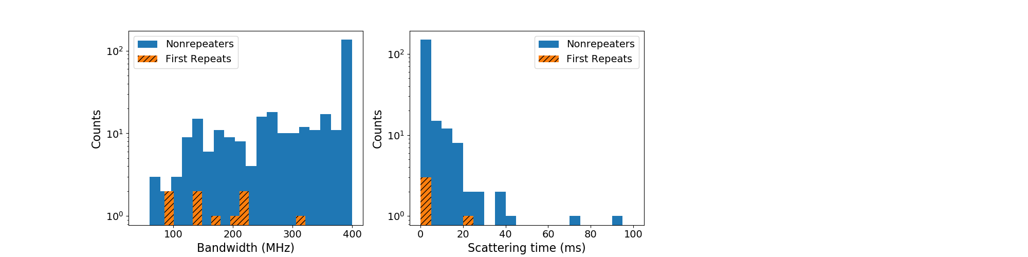
Figure 15: (Left) Distribution of bandwidth for first-detected repeater events and for apparent non-repeaters. Note that bandwidths have not been corrected for instrumental response, which is complex and strongly dependent on declination and location in the detection beam, but on average, is identical for non-repeaters and repeaters. The distributions are inconsistent with arising from the same underlying sample ($p_{AD}=1.3\times 10^{-4}$, $p_{KS}=2.3\times 10^{-4}$). (Right) Distributions of scattering times for first-detected repeater events and apparent non-repeaters for which the time scale was measurable. Upper limits are not included in the plot. For repeaters, the scattering time plotted is the most constraining of those measured of all repeat bursts (but still not plotting upper limits). The samples are statistically consistent with arising from the same underlying distributions.

We can also compare distributions of scattering times for apparent non-repeaters and repeaters in Catalog 1. A difference might be expected if the local source environment between repeaters and non-repeaters differed, and if scattering in the local environment dominated over other sources of scattering. Figure 15 (right) shows measured scattering times (ignoring upper limits) for the repeaters and apparent non-repeaters. For repeaters, the scattering time plotted is the most constraining from all of the sources’ repeat bursts. Our statistical tests indicate no evidence for the distributions being from different underlying populations ($p_{AD}=0.42$, $p_{KS}=0.32$). We also verified this result using the log-rank test and the modified Gehan-Wilcoxon test. Both tests yielded $p$-values indicating consistent underlying populations, with $p=0.1$ and 0.3, respectively.

A correlation between scattering times and extragalactic DMs might be expected if scattering is dominated by a component in the intergalactic medium and extragalactic DMs are not dominated by host contributions, or conversely if both scattering and extragalactic DM are dominated locally at the source. Any correlation detected in Catalog 1 requires correction due to instrumental biases as discussed below (Section 6.1). However, such biases should be the same for non-repeaters and repeaters so it is fair to ask here whether similar correlations exist for both groups. To investigate, we compared the 2D scattering time versus extragalactic DM distributions for apparent non-repeaters and for first-detected repeaters using the 2DKS test, and found that they are consistent with the distributions originating from the same underlying population ($p_{2DKS}=0.10$). However, the sample size for first-detected repeaters is small and minor distribution differences might be yet undetectable. Inclusion of $\mathrm{SNR}<12$ events yields no interesting difference. We will report on a more detailed analysis of this possible correlation in future work, but discuss it briefly in Section 7.3.

5.5 Summary of repeater vs apparent non-repeater comparisons

In summary, we find strong evidence for significant differences in the intrinsic burst widths and bandwidths of repeating FRBs compared to a population yet to be seen to repeat. In contrast, we do not find significant differences when comparing the two populations for sky distribution, DM and scattering distributions, or signal strengths. A summary of the results of our comparison are provided in Table 3.

Table 3: Summary of Repeater vs Apparent Non-Repeater Distribution Comparisons

Property	§	Figure No.	$p_{AD}^{a}$	$p_{KS}^{b}$	$p_{2DKS}^{c}$
Right Ascension	5.1	10	0.22	0.24	…
Declination	5.1	10	0.55	0.49	…
DM	5.2	11	0.35	0.33	…
eDMd	5.2	11	0.34	0.24	…
bonsai SNR	5.3	12	0.65	0.44	…
fitburst SNR	5.3	12	0.08	0.26	…
Fluence	5.3	13	0.070	0.066	…
Flux	5.3	13	0.028	0.068	…
2D fluence vs eDM	5.3	…	…	…	0.099
2D flux vs eDM	5.3	…	…	…	0.43
Widthe	5.4	14	$7.3\times 10^{-5}$	$5.6\times 10^{-5}$	…
Boxcar width	5.4	14	$1.5\times 10^{-4}$	$2.2\times 10^{-4}$	…
Bandwidth	5.4	15	$1.3\times 10^{-4}$	$2.3\times 10^{-4}$	…
Scattering timee	5.4	15	0.42	0.32	…
2D scattering timee vs eDM	5.4	…	…	…	0.10

Notes.
^aAnderson-Darling probability of originating from same underlying population
^bKolmogorov-Smirnov probability of originating from same underlying population
^c2D Kolmogorov-Smirnov probability of originating from same underlying population
^dExtragalactic DM
^eexcludes upper limits; results qualitatively the same when including them – see text.

6 Intrinsic characteristics of the FRB population

Here we infer the properties of the intrinsic FRB population from the observed CHIME/FRB Catalog 1 data. The central challenge is to account for selection biases, i.e., the fact that the probability to detect an FRB depends on its properties in a complicated way, and to account for instrument-induced errors in the measured quantities. To correct the observed property distributions for these effects, we use the injection system described in Section 4. Here we give a brief overview of the methods used to account for selection effects. A more detailed description of our FRB inference pipeline, including additional methods used for cross-checks, will be described elsewhere. We present distributions of FRB properties corrected for selection biases and perform a more detailed examination of the data in the property space of fluence and DM: inferring the overall FRB sky rate, the fluence distribution, and examining how the fluence distribution depends on DM.

For the present population analysis, we will consider six FRB properties: fluence ($F$), DM, scattering timescale ($\tau$), intrinsic width ($w$), spectral index ($\gamma$), and spectral running ($r$). Using injections to compensate for selection effects is complicated by the fact that both the selection effects, and the intrinsic FRB population, may be correlated in the high-dimensional phase space of FRB properties. For instance, we expect a selection bias against high-DM bursts because DM-smearing dilutes the burst signal in time. However, this bias is weaker if FRBs have a wider intrinsic pulse profile since the smearing would then have a smaller relative effect. It is also weaker if FRBs have flatter spectra, since a larger fraction of the signal would come from higher frequencies where the effect of smearing is reduced. There is also an interplay with signal loss from our data filtering and flagging, which more adversely affects low-DM events. Thus, in principle, the distributions of all three of these properties (and in fact all FRB properties) should be modeled and fit simultaneously to be fully consistent.

We instead make a number of simplifying assumptions, and defer a full multi-dimensional intrinsic correlations analysis to future work. To simplify the analysis, we study FRB properties one or two at a time, holding the distributions for the rest of the properties fixed at a fiducial population model that provides a reasonable overall description of the data. As we show in the next section, it is possible to robustly compensate for correlations in the selection effects so long as correlations in the intrinsic population are small.

6.1 Selection bias-corrected FRB property distributions

First, we set up our formalism and outline our procedure. We wish to make inferences about the intrinsic property rate function of these FRBs: $R(F,\mathrm{DM},\tau,w,\gamma,r)$. However, observational effects mean that not all regions of property space are observed with the same efficiency. We define the observation function to be $P(\mathrm{SNR}|F,\mathrm{DM},\tau,w,\gamma,r)$, which describes the stochastic mapping from event properties to SNR (the stochastic mapping is because of a burst’s random location in the beam and occurrence relative to time-variable effects such as RFI). In our usage, the observation function is averaged over time and sky location, and is affected by the beam, system sensitivity, detection pipeline efficiency, RFI, and other effects.

Our main simplifying assumption is that the FRB properties are intrinsically uncorrelated (other than $\gamma$ and $r$ for which we observe strong correlations) such that their distributions factorize:

$$R(F,\mathrm{DM},\tau,w,\gamma,r)=R_{0}P(F)P(\mathrm{DM})P(\tau)P(w)P(\gamma,r),$$ (3)

where $R_{0}$ is the overall sky rate (with units events per sky per day) and the other factors are the individual probability density functions for each property. Rigorously testing this assumption is beyond the scope of this paper and will be deferred to future work, except for $F$ and $\mathrm{DM}$, which we study briefly in Section 6.2. Given the limited statistical power of our sample of $\sim 250$ events, we expect such correlations to have a small impact on our results. We do, however, check for intrinsic correlations through a series of jackknife tests described in Section C.3, finding some evidence that such correlations may exist.

One complication is that the fluence we measure for a given event is a highly uncertain estimate of the true fluence (due primarily to the uncertain localization and beam sensitivity, see Section 3.4). In addition, we do not currently have the ability to robustly forward model the fluence measurement processes using the injections system. For these reasons, we do not use fluence measurements for our inferences. We can nonetheless make inferences about the intrinsic fluence distribution since the detection SNR (which is robustly modeled using injections) strongly correlates with fluence. Although it has been shown that under certain assumptions SNR and fluence are distributed with the same power-law index (Oppermann et al., 2016; Connor, 2019; James et al., 2019), our analysis does not rely on this result, only requiring that fluence and SNR correlate. Integrating out the fluence, the observed rate of FRBs is:

$$\mathcal{R}_{\rm obs}(\mathrm{SNR},\mathrm{DM},\tau,w,\gamma,r)=\int_{0}^{\infty}dF\,P(\mathrm{SNR}|F,\mathrm{DM},\tau,w,\gamma,r)R(F,\mathrm{DM},\tau,w,\gamma,r),$$ (4)

where $\mathcal{R}_{\rm obs}$ denotes the observed, as opposed to the intrinsic, rate function.

The observed distribution of any single property is the integral over the other properties including property ranges within any cuts made on the data. For example, the observed distribution of DM would be:

$$P_{\rm obs}(\mathrm{DM})\propto\int_{\mathrm{SNR}_{\rm thres}}^{\infty}d\mathrm{SNR}\,\int d\tau\,dw\,\,d\gamma\,dr\,\mathcal{R}_{\rm obs}(\mathrm{SNR},\mathrm{DM},\tau,w,\gamma,r),$$ (5)

which—given our assumption of uncorrelated intrinsic distributions—can be corrected to the intrinsic distribution:

$$P(\mathrm{DM}) =P_{\rm obs}(\mathrm{DM})s(\mathrm{DM})^{-1},$$ (6)

$$s(\mathrm{DM}) \propto\int_{\mathrm{SNR}_{\rm thres}}^{\infty}d\mathrm{SNR}\int d\tau\,dw\,d\gamma\,dr\,dF\,P(\mathrm{SNR}|F,\mathrm{DM},\tau,w,\gamma,r)P(F)P(\tau)P(w)P(\gamma,r),$$ (7)

where the constant of proportionality in the second line is set by the requirement that the intrinsic distribution, $P(\mathrm{DM})$, and the observed distribution, $P_{\rm obs}(\mathrm{DM})$, be normalized. Above, $s(\mathrm{DM})$ is the DM selection function, i.e., the probability for an FRB with a given DM to be detected, marginalized over all other FRB properties.

Note that under our assumption of uncorrelated intrinsic distributions, $s(\mathrm{DM})$ does not in itself depend on the intrinsic distribution of FRB DMs (see Eq. 7), but does depend on the intrinsic distributions of the other properties. However, if $P(\mathrm{SNR}|F,\mathrm{DM},\tau,w,\gamma,r)$ factorizes into separate functions of the FRB properties, this dependence vanishes. In practice we expect that most selection effects induce correlations in the observed sample at the $\lesssim$10% level, although we defer a detailed study of these correlations to future work. This dependence generalizes to other properties: for property $\xi$, $s(\xi)$ is independent of $P(\xi)$ and depends on $P$ of the other properties only through correlations in the observation function, which we expect to be modest.

Having argued that the selection function should be weakly dependent on the underlying intrinsic property distributions, we can calculate an accurate selection function given a fiducial model (hereafter denoted with the subscript “fid”, e.g. $R_{\textrm{fid}}$, $P_{\textrm{fid}}$) for the FRB property distributions that is a reasonable, albeit imperfect, match to the data. Likewise, below we study the FRB population in the property subspace of DM–$F$, fixing the other properties at the fiducial model. Our results for a given property distribution (e.g., the DM distribution) should thus be interpreted in the context of a weak dependence on our model for other properties (e.g., the scattering distribution) as well as our overall assumption of uncorrelated intrinsic properties.

In Appendix C we detail our assumed functional forms for the property distribution functions appearing in Equation 3 and our procedure for using injections to find fiducial model parameters that match our observations. Here we describe only the details that are critical to understanding further results. Rather than iteratively injecting a new population for every candidate model we wish to test, we use property dependent weights $W(F,\mathrm{DM},\tau,w,\gamma,r)$ to convert a single injected population to any other population model.

We find that, due to a strong selection bias against highly scattered events, the population with scattering time above 10 ms is very poorly constrained. In order for this part of the population to not dominate uncertainties, we cut them from further analysis except for the measurement of $s(\tau)$, which is independent of $P(\tau)$. In addition, at low $\tau$ and $w$, there is significant measurement uncertainty in these properties, with many measurements in the $\sim 1$ ms range being upper limits. We deal with this uncertainty by using wider $0.5$ ms bins below 2 ms, and assigning a value of half the 2$\sigma$ upper limit where these occur ($24$ events for $w$ and $257$ events for $\tau$, before cuts). This treatment is far from ideal, but is likely sufficient since the purpose of the fiducial model is only to roughly describe the property distributions for dealing with correlations in the selection effects.

We exclude 39 events that are detected either during pre-commissioning, epochs of low-sensitivity, or on days with software upgrades. In the catalog data these events are noted in the excluded_flag field.

After applying the cuts discussed in Section 5, the cuts on $\tau>10$ ms, and the cuts on days with system concerns, the remaining sample still contains repeaters, with multiple bursts making these cuts. For these sources, only the first burst is kept; all subsequent events are excluded from the analysis. We do this because for some properties (DM, scattering), repeat bursts from the same source should have the same value. Including repeat bursts would thus skew the statistics of our distributions. As such, we are effectively studying the distributions of sources rather than bursts, a small but conceptually important distinction.

The post-cut sample includes $22$ events with complex morphology and thus no unique value of $w$. For these events, we estimate an “effective” pulse width by using a value proportional to the boxcar width, with the constant of proportionality (equal to 0.17) calibrated by comparing the pulse widths and the boxcar widths of single-component events.

We consider only the DM range in excess of 100 pc cm^-3, since even after classifying events using the Galactic DM models, the extragalactic nature of sources below 100 pc cm^-3 is somewhat ambiguous. This restriction excludes no FRBs from the Catalog 1 sample but does exclude a number of injected events. In total, 270 Catalog 1 events were excluded (265 events remained) after applying the above cuts.

The injections and fiducial model are used to calculate selection functions for the properties DM, $\tau$, and $w$. These are shown in Figures 16, 17, and 18, along with both the uncompensated and selection-compensated distributions for the properties of observed events.

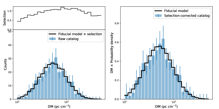
Figure 16: DM distribution before (left) and after (right) compensating for selection effects. Blue histograms are the catalog data with error bars representing the Poissonian 68% confidence interval on the underlying bin mean. When plotted as a probability density in the right panel, the quantity $\mathrm{DM}\times P(\mathrm{DM})$ is unitless and is equivalent to the probability density function re-parameterized in terms of $\ln\mathrm{DM}$. This scaling aids in visual interpretations of the area under the probability density when using a logarithmic horizontal axis. The selection function plotted in the top left is normalized such that Equation 6 holds for the fiducial model. The fiducial model is the best-fit log-normal distribution resulting from the iterative fitting procedure described in Section C, with the appropriate selection function applied as per Equation 7. The selection function varies by more than a factor of two over the range of observed DMs, with biases against low-DM events from detrending and flagging being a larger effect than that of DM smearing affecting high DMs. A log-normal function provides a good description of the data once accounting for selection effects.

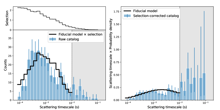
Figure 17: Scattering time ($\tau$, scaled to 600 MHz) distribution before (left) and after (right) compensating for selection effects. Histogram, error bar, and line meanings are analogous to Figure 16. Because of the poorly constrained, apparently rising distribution, the gray region with scattering above 10 ms is not included in fiducial model fit, subsequent analysis, or histograms of other properties. Nonetheless, the selection function is valid in this region. To account for uncertainty in the scattering time measurement, the fiducial model is fit using bins that are wider than those shown here, with linear bins of width 0.5 ms up to 2 ms and logarithmic bins thereafter. To events for which only an upper limit on scattering is measured, we assign a value of 1/2 the 2$\sigma$ upper limit. The log-normal fit for the fiducial model is a marginal match to the data, although the data are affected by observational uncertainties and the large portion of events for which we measure only upper limits. We find there is severe selection bias against events with scattering time larger than 10 ms and the handful of highly scattered events we observed imply there may be a substantial unobserved population of highly scattered FRBs.

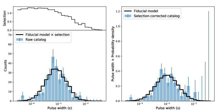
Figure 18: Intrinsic width ($w$, defined as $\sigma$ of a Gaussian profile) distribution before (left) and after (right) compensating for selection effects. Histogram, error bar, and line meanings are analogous to Figure 16. Complex-morphology bursts are assigned an effective width as described in Appendix C. The treatment of measurement uncertainty for fitting (linear 0.5-ms-wide bins below 2 ms) and upper limits is the same as in the scattering case. While there is a strong selection bias against wide events, we find a log-normal distribution to be a satisfactory fit for the full range of widths, with little evidence for an unobserved, intrinsically very wide population.

In cases where intrinsic correlations might be expected, it is instructive to plot events in property subspaces. Motivated by the jackknife tests in Appendix C.3, we show a number of these subspaces in Figure 19. Note that when viewed in this way, intrinsic correlations (as opposed to correlated selection effects) should manifest as discrepancies between the catalog sample and the intrinsically uncorrelated fiducial model (which may have selection-induced correlations). Our ability to measure the properties of catalog bursts complicates this comparison, although no such correlations are visually obvious. The exception might be SNR and $\mathrm{DM}$, for which there is a deficit of events at high DM and high SNR compared to the fiducial model. We study this in more detail in Section 6.2.

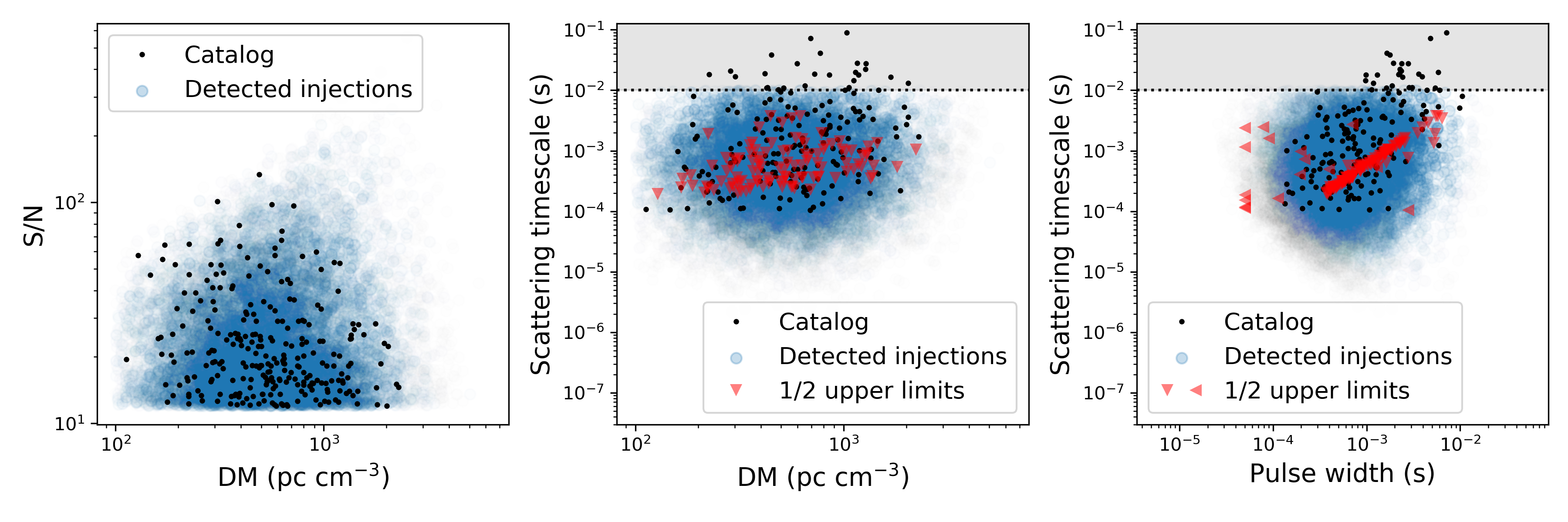
Figure 19: Catalog 1 events in a few property subspaces compared to the fiducial model with selection effects included. For injected events, the opacity is proportional to the weight derived from the fiducial model $W(F,\mathrm{DM},w,\tau)$. Cases for which we only measure upper limits on a property are plotted at half the upper-limit value, and are denoted with red triangles. Property measurement effects (which are distinct from selection effects) are apparent here. Particularly, for cases where no scattering is detected we have assigned an upper limit equal to 2 times the width (see Section 3.3).

As mentioned above, the spectral index ($\gamma$) and spectral running ($r$) parameters are observed to be strongly correlated and due to the observed complexity in this space, we do not attempt to fit a functional form to $P(\gamma,r)$. Instead we use kernel density estimation directly on the catalog measurements. Here, there is potential for a large mismatch between the observations and the fiducial model once accounting for selection biases using injections. Indeed, in the left panel of Figure 20, the catalog spans a larger space of spectral parameters than the detected injections. Fortuitously, forward modeling the measurement process of the spectral properties of the detected injections makes them a better match to the catalog. Each injected burst has an associated “intrinsic” spectral parameter. After going through the injections system, the fluence spectrum gets modulated by the beam model and “measured” spectral properties $\gamma$ and $r$ are fit. These measured properties are more directly comparable to the catalog values. The right panel of Figure 20 shows these to be a reasonable match to the catalog distribution.

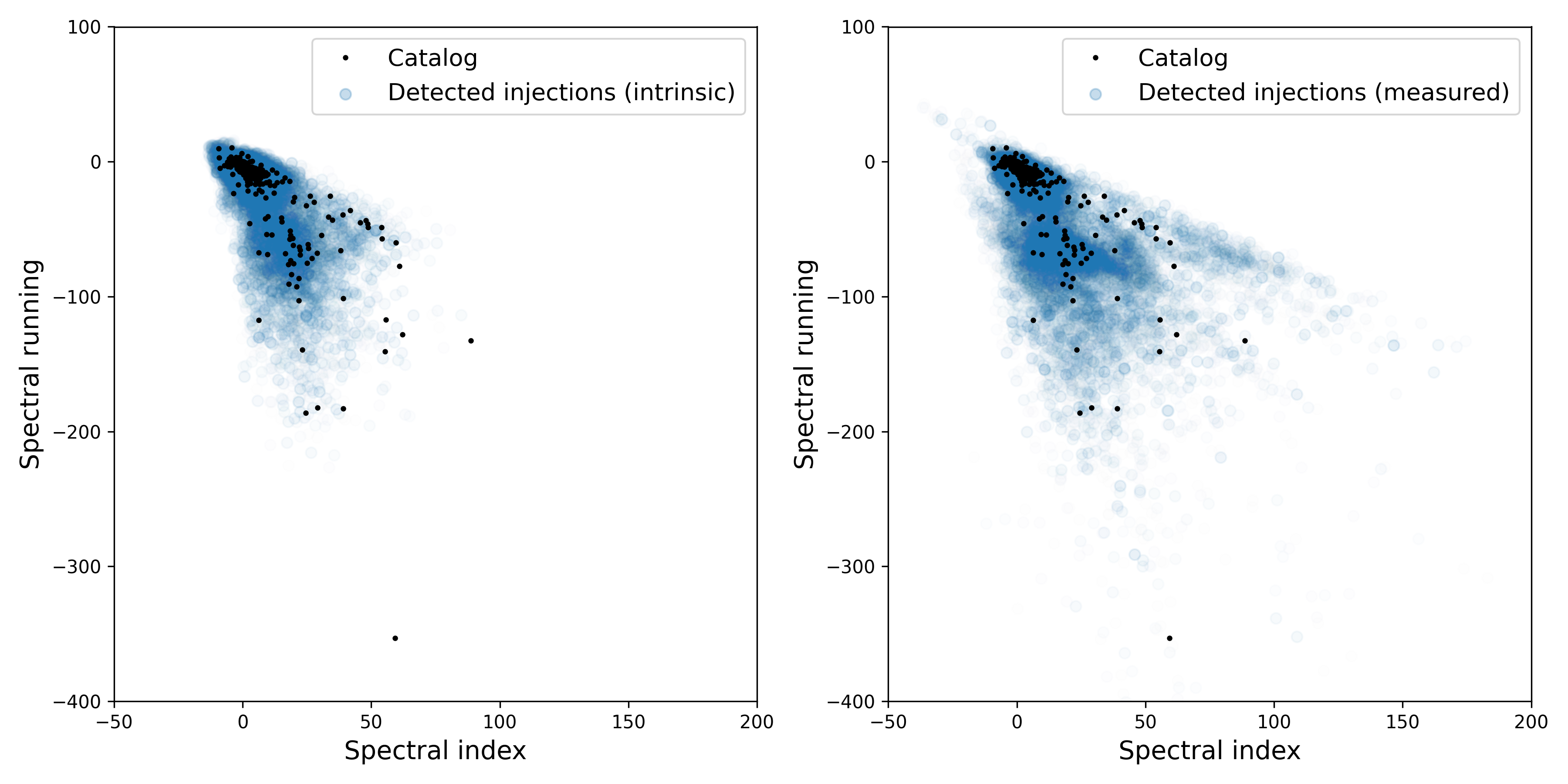
Figure 20: Spectral index ($\gamma$) and spectral running ($r$) for the catalog and detected injection events. Each data point represents a single event, with the Catalog 1 data identical in both panels. In the left panel, we plot the intrinsic spectral parameters of the injected event, and in the right panel we plot recovered spectral parameters after simulating the measurement processes using a model for the telescope beam. For injected events, the opacity is proportional to the weight derived from the fiducial model $W(F,\mathrm{DM},w,\tau)$. The detected injections sample provides a reasonable match to the spectral parameters of the catalog events, especially after accounting for the measurement process. Bursts with multiple subcomponents from the catalog (which have multiple values of $\gamma$ and $r$) are omitted in this comparison.

6.2 Fluence distribution and sky rate

Here we perform a detailed study of the fluence distribution of FRBs, including a measurement of the absolute rate on the sky. We parameterize the fluence distribution by $\alpha$, the power-law index for the cumulative distribution such that the number of events occurring above some fluence threshold is $N(>F)\propto F^{\alpha}$. We study our population in the property space of fluence and DM (with SNR as the observable proxy for fluence). This is motivated by the fact that we expect DM to be strongly correlated with distance, as in the Macquart relation (Macquart et al., 2020), which should in turn induce intrinsic correlations between DM and fluence. Our data are thus the number of counts $N_{ij}$ in the 2D histogram of the catalog (including 265 events after cuts) in SNR bins labeled by index $i$ and DM bins labeled by index $j$.

Our first step in modeling the data in this space is to compute the observation function marginalized over the other FRB properties using fiducial distributions:

$$P(\mathrm{SNR}|F,\mathrm{DM}) =\int d\tau\,dw\,d\gamma\,dr\,P(\mathrm{SNR}|F,\mathrm{DM},\tau,w,\gamma,r)P_{\rm fid}(\tau)P_{\rm fid}(w)P_{\rm fid}(\gamma,r)$$ (8)

$$=\frac{\int d\tau\,dw\,d\gamma\,dr\,P(\mathrm{SNR}|F,\mathrm{DM},\tau,w,\gamma,r)R_{\rm fid}(F,\mathrm{DM},\tau,w,\gamma,r)}{\int d\tau\,dw\,d\gamma\,dr\,R_{\rm fid}(F,\mathrm{DM},\tau,w,\gamma,r)}.$$ (9)

In Equation 9, both the denominator and the numerator are estimated from histograms of the injections and detected injections respectively, using fiducial-model weights. Note that $P_{\rm fid}(F)$, $P_{\rm fid}(\mathrm{DM})$, and $R_{0}$ cancel out in this expression, although care must be taken to properly account for factors of $f_{\rm sky}$ and $\epsilon_{\rm inj}$ introduced when generating the injections population (see Section 4.1.2). As a three-dimensional function, this observation function is difficult to visualize; however, Figure 21 shows its cumulative version, integrating out the DM dependence. We term this the all-sky completeness, given by

$$c(\mathrm{SNR}_{\rm min},F)\equiv\int_{\mathrm{SNR}_{\rm min}}^{\infty}d\mathrm{SNR}\int d\mathrm{DM}\,P(\mathrm{SNR}|F,\mathrm{DM}).$$ (10)

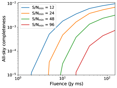
Figure 21: Injections-calibrated all-sky completeness as a function of fluence and minimum SNR included in the sample. Properties other than fluence are drawn from the fiducial property model, with the precise equation for the completeness given in Equation 10. Plotted lines are ordered top to bottom in the same order as the legend. For high-fluence events, the completeness above $\mathrm{SNR}=12$ is of order 0.5% which can be understood since CHIME/FRB’s half-power field of view is roughly 0.3% of the sky at 600 MHz.

With the required observation function in hand, a prediction can be made for the DM–SNR distribution of the catalog

$$\mathcal{R}_{\rm obs}(\mathrm{SNR},\mathrm{DM}|\boldsymbol{\lambda})=R_{0}\Delta t\int dFP(F,\mathrm{DM}|\boldsymbol{\lambda})P(\mathrm{SNR}|F,\mathrm{DM}),$$ (11)

for a given model $P(F,\mathrm{DM}|\boldsymbol{\lambda})$ depending on parameters $\boldsymbol{\lambda}$ (described below). Here, $\Delta t=214.8$ days is the survey duration. Our prediction for the data $N_{ij}$ is then just this function discretized into finite bins:

$$\mu_{ij}(\boldsymbol{\lambda})=\Delta\mathrm{SNR}_{i}\,\Delta\mathrm{DM}_{j}R_{0}\,\Delta t\int dF\,P(F,\mathrm{DM}_{j}|\boldsymbol{\lambda})\,P(\mathrm{SNR}_{i}|F,\mathrm{DM}_{j}).$$ (12)

For fitting the model to the data, we use the binned Poisson likelihood (Zyla et al., 2020):

$$\ln[\mathcal{L}(\boldsymbol{\lambda})]=-\sum_{ij}\left\{\mu_{ij}(\boldsymbol{\lambda})-N_{ij}+N_{ij}\ln\left[\frac{\mu_{ij}(\boldsymbol{\lambda})}{N_{ij}}\right]\right\}+\textrm{constant}.$$ (13)

As a first model, we assume the fluence-DM distribution factorizes into a power law in $F$ and a free function of DM:

$$R_{0}P(F,\mathrm{DM}_{j}|\boldsymbol{\lambda})\,\Delta t\,\Delta\mathrm{DM}_{j}=-\alpha\left(\frac{F}{F_{0}}\right)^{\alpha-1}\frac{\eta_{j}\Delta t}{F_{0}}.$$ (14)

Here, $F_{0}$ is an arbitrary pivot fluence, and the parameter vector $\boldsymbol{\lambda}$ contains $\alpha$ and a log rate per DM bin $\ln\eta_{j}$. In this parameterization $R_{0}$ is a derived parameter proportional to $\sum_{j}\eta_{j}$, the latter of which is the rate of events above the $F_{0}$.

We choose logarithmically spaced bins in $\mathrm{SNR}$ and DM with $12$ bins covering an SNR range of 12 to 200 and $16$ bins covering a DM range of 100 pc cm^-3 to 2800 pc cm^-3, covering the full post-cut Catalog 1 sample. The integral in Equation 12 is performed with Riemann sums, with $P(\mathrm{SNR}_{i}|F,\mathrm{DM}_{j})$ estimated from fiducial-model injections in 100 logarithmic bins covering 0.2 Jy ms to 50 Jy s. We choose a pivot scale $F_{0}=5$ Jy ms, which is substantially higher than the minimum fluence CHIME can detect, $\sim 1$ Jy ms. Choosing this higher pivot scale substantially reduces the statistical correlations between the inferred rate and $\alpha$. We employ uniform priors on our parameters such that the likelihood in Equation 13 is proportional to the posterior.

To validate the procedure outlined above, we apply it to a suite of randomly chosen subsamples drawn from detected injected events in place of Catalog 1 events. In these tests, we use initial distributions instead of fiducial distributions in Equation 9 since the scattering, widths, and spectral parameters of the injections are drawn from these initial distributions. In all trials we are able to recover the injected fluence distribution (for which $\alpha=-1$) within statistical uncertainties. This validation remained true when increasing the sample size to 4000 in order to reduce statistical uncertainties and search for biases.

In Appendix D we do an accounting of systematic errors in this measurement. These final systematic errors are dominated by our rough estimate of the effect of intrinsic property correlations, as assessed through jackknife tests in the fiducial model fitting procedure (see Appendix C). For the rate, uncertainty in the beam model is also significant. The net systematic uncertainty for the rate is ${}^{+27\%}_{-25\%}$ and for $\alpha$ it is ${}^{+0.060}_{-0.085}$.

Figure 22 shows $N_{ij}$ summed over DM bins $j$ as well as $\mu_{ij}$ for the best-fit parameters. Markov-Chain Monte Carlo (MCMC) samples of the posterior, generated using the emcee package (Foreman-Mackey et al., 2013) are also shown. We find $\alpha=-1.40\pm 0.11({\rm stat.})^{+0.06}_{-0.09}({\rm sys.})$, and the rate $\sum_{j}\eta_{j}=[525\pm 30({\rm stat.})^{+140}_{-130}({\rm sys.})]~{}{\rm sky}^{-1}~{}{\rm day}^{-1}$, above a fluence of 5 Jy ms, with a scattering time at $600$ MHz less than 10 ms and above a DM of 100 pc cm^-3.

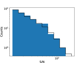
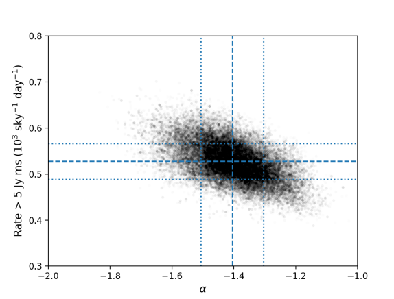
Figure 22: Fits to the FRB rate and fluence distribution. (Left) histogram of the detection SNR and a model fit that includes a DM-dependent probabilistic mapping from fluence to SNR calibrated from injections. (Right) Markov-Chain Monte Carlo samples for the model-fit posterior distribution. Model parameters are the all-sky rate of FRBs with fluence above 5 Jy ms and the cumulative fluence distribution index $\alpha$. Dashed lines show the mean parameter values and dotted lines span $\pm 1\sigma$ statistical uncertainty. The distribution includes bursts DM above $100$ pc cm^-3 and with scattering times less than 10 ms at 600 MHz. Not included in the distributions is a systematic error of ${}^{+27\%}_{-25\%}$ on the rate, and ${}^{+0.06}_{-0.09}$ on $\alpha$. This constitutes a statistically precise measurement of the FRB rate in the CHIME band and at this fluence scale, and indicates the fluence distribution is consistent with the Euclidean expectation of $\alpha=-3/2$.

We note that the resulting value of $\alpha$ is not identical to that fit for the fiducial model, which contains the same parameter, in Appendix C. However, the analysis in this section is more thorough, with notable differences being: 1) we are using a different model for the DM distribution; 2) we are simultaneously fitting DM and fluence distributions; and 3) we are sampling the likelihood using MCMC instead of maximum likelihood. Because of this, differences in best-fit values of a fraction of a $\sigma$ are expected.

To understand our rate measurement, it is instructive to determine a rough expectation based on our injections-calibrated completeness shown in Figure 21. This expectation is a strong function of both the fluence of the burst and the SNR threshold for inclusion in the sample. We see that even for very bright bursts with fluence $\sim 100$ Jy ms, our completeness is below 1%. This result is not surprising since CHIME/FRB’s field of view is about 0.3% of the sky. For our chosen SNR threshold of 12, the completeness is sharply rising at a fluence of $\sim 5$ Jy ms so we are mainly sensitive to bursts above this level. If we take $c(F=10\,\textrm{Jy\,ms})\sim 1\times 10^{-3}$ as a representative value, we obtain a rate of $N/(\Delta t\,c)\sim 1200\,{\rm sky}^{-1}\,{\rm day}^{-1}$, above a fluence of 5 Jy ms, close to the value obtained from the full analysis.

To search for distance-scale induced correlations between fluence and DM (as suggested by our catalog events prior to correction for selection biases—see Section 5.3), we subdivide our sample by DM, splitting at $\mathrm{DM}=500$ pc cm^-3, which is close to the median value of our catalog after cuts. As shown in Figure 23, the low-DM sample has $\alpha=-0.95\pm 0.15({\rm stat.})^{+0.06}_{-0.09}({\rm sys.})$ whereas the high-DM sample has $\alpha=-1.76\pm 0.15({\rm stat.})^{+0.06}_{-0.09}({\rm sys.})$. Noting that the systematic error should be mostly common between the two samples, the difference between them is significant at the 3.8$\sigma$ level.

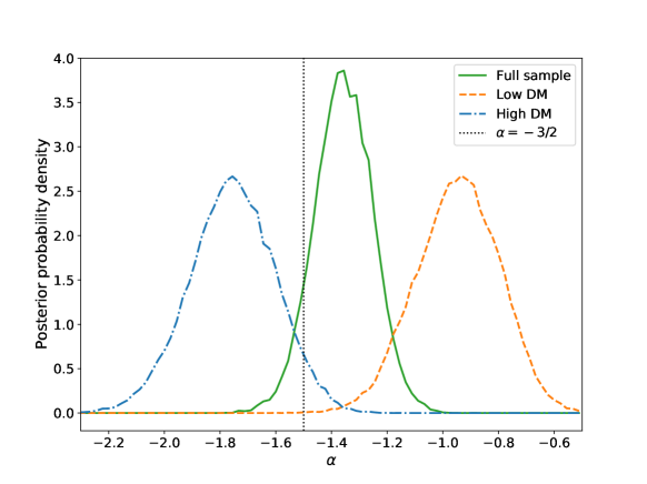
Figure 23: Marginalized posterior distributions for the fluence distribution index $\alpha$ for different ranges of DM. The low DM range is $100$ to $500$ pc cm^-3 and the high DM range is above $500$ pc cm^-3. Not included is a systematic uncertainty of ${}^{+0.030}_{-0.085}$ pc cm^-3, which is shared amongst DM ranges. When considering nearly the full range of DM detectable by CHIME/FRB, the fluence distribution is consistent with being Euclidean, as expected for a population dominated by source redshifts less than $z=1$. However, $\alpha$ is significantly steeper for high-DM events than for low-DM events. This is consistent with the expectation that high-DM events are more distant and we thus preferentially sample the high end of the luminosity function, which, if well behaved, must be steeper than the low end (see Section 7.4).

Properly accounting for the observation function $P(\mathrm{SNR}|F,\mathrm{DM})$ is critical to making this measurement, and shown in Figure 24. It can be seen that the SNR distribution of the catalog events is not strikingly different for the low-DM and high-DM sample. However, the low-DM events have a shallower mapping from fluence to SNR. This is somewhat expected since our wideband RFI mitigation clips significant signal from very bright events, an effect which is substantially stronger at low DM.

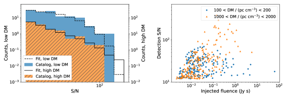
Figure 24: Data and selection effects leading to the fluence distribution measurements in the high and low DM ranges. (Left) Histogram of the detection SNR and a model fit that includes selection effects, as in the left panel of Figure 22, and with vertical scales offset for clarity. The low DM range is $100$–$500$ pc cm^-3 and the high DM range is $>500$ pc cm^-3. The fit model for the low-DM events appears to be steeper than that for the high-DM events, despite being derived from a fit value of $\alpha\sim-1$ compared to $\alpha\sim-2$. The apparent inconsistency is due to a DM-dependent probabilistic mapping from fluence to SNR which we have calibrated from injections. This is illustrated in the right panel, which shows the SNR and fluence of 200 injected and subsequently detected events in each of two DM ranges, drawn from otherwise identical property distributions. It can be seen that our detection system has a shallower mapping from fluence to SNR for low-DM events compared to high-DM events, with very few low-DM events achieving an SNR above 100. This latter effect is likely due to our wideband RFI mitigation strategies, which preferentially remove signal from bright, low-DM events.

7 Discussion

Our first CHIME/FRB catalog presents 536 FRB events, detected over a 371-day period, of which 492 are unique sources, and 18 are repeating sources. This is the largest catalog of FRBs detected by a single instrument, allowing their characterization in the context of a single set of carefully studied selection biases. We have measured burst properties in a systematic, uniform way. As such, the catalog represents a unique resource for studying the FRB population, such as statistical comparisons between repeaters and apparent non-repeaters, and the determination of the fluence distribution and rate of FRBs, as presented in this work. Additional analyses of the catalog data are ongoing, including a study of repetition statistics, as well as a volumetric rate analysis. We also have archived complex voltage data on many of the FRBs in this catalog; the analysis of these data is ongoing and beyond the scope of this paper, but will permit polarimetry, high time- and frequency-resolution studies of burst morphology, as well as improved localizations for the relevant bursts.

In what follows, we discuss the main results of this paper, namely the repeater versus apparent non-repeater comparison, the intrinsic DM, width and scattering distributions, as well as the fluence distribution and rate.

7.1 Are repeaters a different FRB population?

In Section 5, we compared distributions of burst properties for repeaters and apparent non-repeaters to determine whether the two groups represent different astrophysical source populations.

In terms of sky distribution, we found no significant difference in right ascension or declination distributions. The latter is perhaps more interesting, given the strong CHIME exposure dependence on declination. Indeed, we find no evidence for a declination-dependence of the first-repeaters to non-repeaters ratio histogram. This exposure. Eventually, we may reach the regime wherein additional exposure no longer results in as many repeating source detections because the majority of the detectable repeaters will have been found, with the brightest and most active repeaters having been found first. We do not yet seem to be in that regime in Catalog 1. Although we have already reported on 18 new repeater discoveries (CHIME/FRB Collaboration et al., 2019c, a; Fonseca et al., 2020), we have in fact detected more and will report on these elsewhere, along with a detailed analysis of the distribution of burst rates.

The DM distributions of repeaters and apparent non-repeaters are consistent with originating from the same underlying distribution. Roughly, with 18 repeating sources, we would expect to be able to detect $\sim 1/\sqrt{18}\sim 25\%$ differences in the mean DM between the samples (at 1-$\sigma$).

If extragalactic DMs are dominated by plasma in the intergalactic medium (e.g., Macquart et al., 2020), then our results suggest no difference between the distribution or host type of repeaters and non-repeaters. On the other hand, if the extragalactic DMs are dominated by the host’s ISM, or its local environment, then the repeaters and non-repeaters must share very similar host properties. In this case, the results from our sample would indicate that any disparities in hosts must coincidentally conspire to yield no significant net different in extragalactic DM distribution between the two types of repeater.

Furthermore, we find no strong evidence for differences in signal strength of repeaters and apparent non-repeaters, nor in scattering properties. In principal it would be instructive to measure $\alpha$ for the two populations separately. However, the spectro-temporal differences between the two populations imply there could be differences in observation biases, making absolute measurements of $\alpha$ challenging for the sub-populations. Also, the repeater sample is still relatively small for a meaningful analysis. In any case, the similarity of the SNR distributions implies there is unlikely to be a statistically significant difference in $\alpha$.

On the other hand, we find strong differences in burst widths and bandwidths, with repeaters having on average significantly broader widths and narrower bandwidths, at least in the CHIME band. The differences are not subtle; they are apparent by eye (see Figs. 14 and 15). They are investigated in more detail by Pleunis et al. (2021, submitted). These differences are strongly suggestive of differing emission mechanisms. This could imply either different source populations, or a single population in which pulse morphology strongly correlates with repeat rate (e.g., Connor et al., 2020).

Different source populations can have identical spatial and local environment properties. For example, some FRBs may have massive stellar progenitors (as in models requiring isolated neutron stars such as magnetars, e.g., Beloborodov, 2017; Margalit & Metzger, 2018), while others may manifest as FRBs due to interactions with a massive companion star (e.g., Ioka & Zhang, 2020; Lyutikov et al., 2020), with both populations found preferentially in regions of star formation within young galaxies. Harder to imagine are examples with one population requiring nearby AGNs (e.g., Thompson, 2017; Vieyro et al., 2017) and another not (most models); such scenarios seem unlikely, given our results, and also given the absence of FRBs near centers of galaxies (Bhandari et al., 2020). Distinct populations in which one is very young (e.g., highly active magnetars; Beloborodov, 2017; Margalit & Metzger, 2018) and the other very old (e.g., colliding compact objects; Yamasaki et al., 2020; Beloborodov, 2020) also seem unlikely for identical spatial and local environment properties. However, the DMs and scattering times of both classes could be heavily dominated by the IGM, and the difference in typical host galaxy type may not be not large.

Conversely, a single population can have sources of vastly different observational emission properties. For example, the Sun itself produces many different types of radio bursts (see, e.g., Kahler, 1992). Perhaps more energetically relevant, radio pulsars exhibit a variety of radio pulse phenomenology, ranging from mode changing and nulling to giant pulses (see, e.g., Manchester & Taylor, 1977; Lorimer & Kramer, 2012). Emission properties in neutron stars can vary with age as well, with young magnetars being highly X-ray and gamma-ray active, but perhaps subsequently evolving to more stable, fainter “Isolated Neutron Stars” (Kaspi, 2010), though in this case, differing local environments would be expected.

Thus, although we have found strong evidence for differing types of emission when comparing repeaters and apparent non-repeaters (see Pleunis et al. 2021, submitted, for further details), it is merely suggestive, but not proof, of different source populations, particularly noting the otherwise similar property distributions.

7.2 Accounting for selection biases

Through an extensive program of signal injections (see Section 4), we have characterized the selection effects in our FRB survey, as described in Section 6.1. So far, we have only injected events using a relatively simple signal model. As such, events with complex pulse shapes or spectral structure may not be adequately characterized. In addition, event properties may be correlated, either due to intrinsic correlations in the population or correlated selection effects. We have mitigated the latter by matching to a fiducial model, such that the observed statistics of the injected sample are a good match to those of the catalog. However, we have explicitly ignored most intrinsic correlations. Another area for concern is that we have assumed a log-normal functional form for the DM, width, and scattering distributions, and only roughly modelled the distributions of the spectral parameters using a kernel density estimator. All of these assumptions are likely highly simplistic compared to reality.

Nonetheless, bursts with complex structure represent a small minority of events, and we believe ignoring correlations in the populations to be a reasonable approximation when estimating the selection function. In addition, our best-fit fiducial model is reasonably well matched to the catalog data as shown in the figures presented in Section 6.1. This indicates our simplistic model provides a decent description at the level of our current statistical precision.

As such, we are able to draw conclusions about the FRB population with unprecedented statistical precision and control of systematics. Further improvements to the multi-dimensional property-space modeling of the FRB population should be a focus of future work in the field as the data continue to become more constraining.

The methods for accounting for selection bias through Monte Carlo-style real-time injections described here are relatively new. Gupta et al. (2021) have implemented an injections system analogous to that used here, although they do not attempt to model the effects of the telescope beam and have not yet propagated their measured selection effects to detailed population inferences. The most complete treatment of FRB selection effects to date was performed by James et al. (2021a, b), who follow an equivalent statistical formalism to that employed here but construct a model for the observation function rather than calibrating it through injections. A failure to account for selection effects will, for any sizable FRB sample, result in incorrect assertions about population distributions. As such, our methods are an important outcome of this work, together with the data presented.

7.3 Intrinsic DM, width, and scattering distributions

From Figure 16, it is clear that the selection effects in DM are modest and that, at least naively, we appear to be detecting the full range of DMs represented in the population detectable at CHIME/FRB’s sensitivity. On one hand, a log-normal distribution peaking at $\sim 500$ pc cm^-3 with tails extending to $\sim 3000$ pc cm^-3 is a good fit; on the other hand, this should be interpreted in the context of our assumption of negligible intrinsic property correlations. The observed DM distribution could be skewed by a correlation between scattering and DM (which is physically well-motivated) or fluence and DM (which we have demonstrated to be present). The latter is of particular concern, since at a lower fluence scale we expect to detect more distant FRBs, having higher DMs.

Interpreting the DM distribution with respect to the Macquart relation (Macquart et al., 2020) taken at face value, roughly half of CHIME/FRB-detected FRB sources have a redshift less than 0.5 with a tail extending to $\sim 2$. However, it is possible that the high-DM tail is dominated by host/source-local plasma and that the maximum redshift probed by our data is considerably lower. Regardless, what is clear is that CHIME/FRB is not detecting many $z>3$ sources so may not be helpful for studies requiring such objects (e.g., Beniamini et al., 2021). Future sensitive, higher-frequency telescopes like the Square Kilometer Array or the CHORD telescope (Vanderlinde et al., 2019) may be useful in this regard.

Unsurprisingly, selection effects in the distribution of intrinsic widths are strong: temporally broad events have a more diluted signal, and many of our RFI mitigation strategies have the effect of filtering out signals with long time-scales from our data. As such, the median width of the population increases by a factor of two once selection effects are accounted for. Nonetheless, even accounting for selection effects, the rate of events with width in the 10 to 20 ms range is small compared to those below 10 ms, and appears to be falling as width increases further (although statistical errors are large in this highly selection-attenuated region). As such, it seems unlikely that there is a large number of FRBs that are undetectable due to large intrinsic width. We urge some caution when making interpretations here, as intrinsic width is the parameter that is most likely to be affected by the limitations of an injection campaign that used only simple burst morphologies. Our inferences about the width distribution are particularly dependent on our assumption that it is uncorrelated with fluence, rather than uncorrelated with intrinsic peak flux (which is proportional to $F/w$). Either assumption is astrophysically well-motivated, and the choice of one over the other depends further on whether FRB emission is an energy-limited or time-limited process. This in itself is an important question that our data should be able to address; however, we defer such an investigation to future work.

In contrast, correcting for selection effects in scattering indicates that there is a substantial population of FRBs with very high scattering that are challenging for CHIME/FRB to observe. In particular, we detected two events with scattering time $>50$ ms and our injections indicate that for these to have been observed, a huge number of highly scattered events must have gone undetected. Indeed, in Figure 17 we do not see much evidence that the event rate is falling in the $10$ to $100$ ms range, and there could be a large population beyond $100$ ms which is essentially unconstrained by our data due to the difficulty of detecting these events. A population synthesis analysis based on the first 13 CHIME-detected FRBs, all of which exhibited scattering timescales $<$10 ms, suggested that FRBs must be located in environments with stronger scattering properties than the Milky Way ISM (CHIME/FRB Collaboration et al., 2019b). We are performing a similar analysis to explore the astrophysical implications of the existence of a large population of highly scattered events, results of which will be presented in future work.

Highly scattered events are easier to detect at higher frequencies due to the steep power-law dependence of scattering time on observing frequency. Scattering timescales have been measured for 18 of the 71 FRBs observed at gigahertz frequencies. Eight of these FRBs have measured scattering times which scale to $>$ 100 ms at 600 MHz, assuming a power-law index of $-$4 for the frequency dependence. Observations of FRBs at frequencies above 1 GHz are thus consistent with the existence of a large population of highly scattered events. We note that the observed number highly-scattered events could also be the result of intrinsic correlations in the population. For instance, if there were a strong correlation between fluence and scattering, we might observe these highly-scattered events without their population being particularly large. However, astrophysically, such a correlation seems unlikely since there is no particular reason fluence, an intrinsic property, should be related to scattering, an extrinsic propagation effect.

A correlation between scattering time and extragalactic DM might be expected, as discussed in Section 5, and would contradict our assumption of independence of these variables (see Section 6). We note that such a correlation is present in the catalog events prior to correction for instrumental biases, though it does not appear strong. As discussed in Appendix C.3, our jackknife tests also hint at a correlation between DM and scattering time after compensating for selection effects. The investigation of the degree of correlation after correction for instrumental biases is beyond the scope of this paper, but will be discussed in future work.

7.4 Fluence distribution

When considering a wide range of DMs, we find the fluence distribution index to be $\alpha=-1.40\pm 0.11({\rm stat.})^{+0.06}_{-0.09}({\rm sys.})$, which is an excellent match to the expected value of $-3/2$ for a non-evolving, constant-density source population in Euclidean space (Herschel, 1785). This agreement is expected, because the peak of our DM distribution is $500$ pc cm^-3, implying a redshift distribution that peaks at $z\lesssim 0.5$. Cosmic evolution of the population, as well as effects from the expansion of the universe, are not expected to result in a significant deviation from the Euclidean expectations at these moderate redshifts.

There have been a number of measurements of the FRB fluence distribution (Oppermann et al., 2016; Vedantham et al., 2016; Amiri et al., 2017; Lawrence et al., 2017; Shannon et al., 2018; Bhandari et al., 2018; Patel et al., 2018), the most recent of which have been consistent with the $\alpha=-3/2$, with some exceptions (Agarwal et al., 2020; James et al., 2019). Agarwal et al. (2020) analyzed a heterogeneous set of surveys, with most data coming from the Parkes (e.g., Thornton et al., 2013; Champion et al., 2016; Bhandari et al., 2018) and Australian Square Kilometre Array Pathfinder (ASKAP) Telescopes (Shannon et al., 2018). They found $\alpha=-0.91\pm 0.34$, a nearly 2$\sigma$ disagreement with the Euclidean expectation. A central challenge of meta-analyses of this type is the comparison of samples from different instruments and surveys. In particular, the effects of beam-model errors tend to cancel in the measurement of $\alpha$ so long as the sample is detected through a single beam (Connor, 2019). James et al. (2019) separately analyzed samples detected at Parkes (finding $\alpha=-1.18\pm 0.24$) and ASKAP (finding $\alpha=-2.20\pm 0.47$) and, while each of these measurements is apparently $\sim$ 1.5$\sigma$ consistent with Euclidean, they asserted that the two populations have different $\alpha$ at the 2.6$\sigma$ level (after accounting for the non-Gaussianity of the likelihoods).

Recently, Lu & Piro (2019) analysed an ASKAP-detected sample, modeling the FRB energy distribution function, redshift evolution of the volumetric rate, and assuming a one-to-one DM-distance relation. In such models, $\alpha$ is a derived quantity that cannot deviate strongly from the Euclidean value except in extreme regions of parameter space or for populations much more distant than the ASKAP sample. Thus, their analysis is not completely comparable to direct fits for $\alpha$, although does better incorporate the astrophysical effects. However, they do find their model to be consistent with the ASKAP fluences once they account for completeness. Likewise James et al. (2021a, b) jointly analysed the Parkes and ASKAP datasets, modeling selection effects, the FRB energy distribution function, and a stochastic DM-distance relation simultaneously. Their best-fit model predicts $\alpha=-1.5$ over most of the observed fluence range, shifting to $-1.3$ for the dimmest (and thus most distant) bursts detectable by Parkes.

Because CHIME/FRB observes at significantly lower frequencies than the 1.4-GHz surveys, it is non-trivial to compare the fluence-scales of the populations seen at Parkes and ASKAP to that of CHIME/FRB. Nonetheless, given that the median DM of the Parkes sample is $\sim 900$ pc cm^-3 compared to $\sim 500$ pc cm^-3 for CHIME/FRB, it is plausible that Parkes is seeing a more distant population than is CHIME/FRB, and is thus seeing cosmological and/or evolutionary effects that flatten the fluence distribution. Indeed, this is the interpretation given by James et al. (2019) and James et al. (2021a, b). However, ASKAP is significantly less sensitive than Parkes and sees a sample with median DM $\sim 400$ pc cm^-3, and yet the James et al. (2019) measurement of $\alpha$ is apparently more discrepant from $-3/2$. Thus, strong departures from the Euclidean value seem difficult to explain for that sample. We note that the $\alpha=-3/2$ expectation holds only after aggregating over FRBs with all DM values and for samples that are complete in DM. We have shown that the DM-completeness of our catalog increases by more than a factor of 2 between $100$ and $1000$ pc cm^-3, an effect for which we have compensated. In addition, the non-linear and stochastic mapping between fluence and SNR had to be carefully calibrated for our measurement. The other analyses listed above have not compensated for either effect and it is unknown whether these effects are strong for the search pipelines at Parkes and ASKAP, although James et al. (2021b) assert them to be negligible.

Splitting the sample by DM, we find that the CHIME/FRB low-DM sample has a significantly shallower slope with $\alpha\approx-1$ compared to the high-DM sample with $\alpha\approx-1.8$. We argue that this too is qualitatively what we would have expected. To understand this, consider the model where DM is exactly proportional to distance. Then, the energy of each FRB is $E=C\,\mathrm{DM}^{2}\,F$ where $C$ is the constant of proportionality. Thus, at fixed DM the joint fluence–DM distribution function, $P(F,\mathrm{DM})$, is directly proportional to the FRB energy distribution function, $n_{E}(E)$:

$$P(F,\mathrm{DM})\propto\mathrm{DM}^{4}\,n_{E}(C\,\mathrm{DM}^{2}\,F),$$ (15)

with the DM-dependent prefactor $\propto\mathrm{DM}^{4}$ coming from the geometry and the change of variables. In order for the total energy output of FRBs ($\sim\int_{0}^{\infty}dE\,E\,n_{E}(E)$) to be finite, the energy distribution must fall more steeply than $E^{-2}$ at high energy and be more shallow than $E^{-2}$ at low energy. Integrating $P(F,\mathrm{DM})$ over DM yields the expected $-3/2$ power law; however, when considering only low-DM events, we preferentially sample the lower end and shallower part of the energy distribution, yielding $\alpha>-3/2$. Likewise for high-DM events, the higher end and steeper part of the energy distribution is preferentially sampled and we obtain $\alpha>-3/2$. Thus, that we observe this expected behavior indicates that we are seeing the distance evolution of the FRB population, sampling different parts of the energy distribution function at different DMs. Note that this interpretation is not necessarily at odds with the interpretation above that Parkes may observe a shallower brightness distribution because it is seeing a more distant, higher-DM population. The Parkes sample is at a different DM and fluence scale than our sample.

Our findings are qualitatively consistent with those of Shannon et al. (2018), who found that the Commensal Real-time ASKAP Fast Transients Survey (CRAFT, which is shallower and wider compared to surveys using the Parkes Telescope) observed a population of FRBs with comparatively lower DMs. The median DM for the CRAFT sample was roughly 400 pc cm^-3 compared to 900 pc cm^-3 for the Parkes sample, which is a factor of 50 more sensitive than CRAFT. It is promising that we can now detect the the DM dependence of the fluence distribution without the complication of comparing heterogeneous surveys.

In principle, we should be able to measure the full energy distribution function: Equation 15 contains an unknown single variate function $n_{E}(E)$ from which we derive a bivariate observable $P(F,\mathrm{DM})$. In practice the fact that DM is a noisy proxy for distance—with a degree of noisiness that has yet to be well established—makes this measurement non-trivial. What we have presented here represents a first step along this path, and we are actively pursuing a more complete analysis.

7.5 FRB rate

In this section we compare our measured sky rate to others published in the literature. We note, however, that we have determined our rate using methods that are quite different from how other rates in literature were estimated, specifically in our forward-modeling of the multi-dimensional selection function (determined using injected bursts; see Section 4), including our complex beam response. Direct comparison with other reported rates is therefore dangerous, since other rate measurements did not account for instrumental effects with the same methods. Nevertheless we proceed with such a comparison, first considering the implications of a simple, naive comparison of published rates, but ultimately recognizing that rate disparities may be a result of different measurement methods and can guide future work on the subject.

As our survey is uniquely in the 400–800-MHz band, we first consider what average spectral index, $\bar{\gamma}$, is reasonable to assume when comparing with rates at other frequencies, where, after accounting for the fluence distribution, the rate scales as

$$R_{5}^{2}=R_{5}^{1}\left(\frac{f_{2}}{f_{1}}\right)^{-\bar{\gamma}\alpha},$$ (16)

where $R_{5}^{n}$ is the rate above 5 Jy ms at radio frequency $f_{n}$. Chawla et al. (2017) constrained the spectral index to be $\bar{\gamma}>-0.3$, fairly flat, using the lack of detections in the 300–400-MHz band from the Green Bank North Celestial Cap (GBNCC) survey and the 1.4-GHz rate from Crawford et al. (2016). This constraint was obtained assuming scattering is important from sources other than the Milky Way and IGM, which seems consistent with our preliminary simulation analyses, to be described in future work. Note that the GBNCC spectral index constraint was not altered by the recent detection of GBNCC’s first FRB (Parent et al., 2020). In contrast, Macquart et al. (2019) report a much steeper spectral index, $\bar{\gamma}=-1.5^{+0.2}_{-0.3}$, based on spectral analysis of 23 ASKAP bursts detected at 1.4 GHz. However, Farah et al. (2019) argue that either ASKAP-derived spectral index is too steep given the low inferred rate from the UTMOST telescope, which operates at 843 MHz, or perhaps there is a spectral turnover below $\sim$1 GHz. Furthermore, non-detections of bright ASPA FRBs at the Murchison Widefield Array (MWA) yielded a constraint $\bar{\gamma}\stackrel{{\scriptstyle>}}{{{}_{\sim}}}-1$ (Sokolowski et al., 2018), also somewhat flatter than the ASKAP value. Here we will start by assuming a simple flat spectral index ($\bar{\gamma}=0$) in the absence of strong evidence otherwise.

Past rate measurements have usually been in the 1.4-GHz band, dominated by the Parkes and ASKAP telescope samples. Here, we consider the most recent measurements only, as early values were based on low statistics. Specifically, Bhandari et al. (2018) report a sky rate of $1.7^{+1.5}_{-0.9}\times 10^{3}$ sky^-1 day^-1 above a fluence limit of 2 Jy ms based on Parkes 1.4-GHz FRB surveys. Shannon et al. (2018) report a rate of $37\pm 8$ sky^-1 day^-1 above 26 Jy ms from ASKAP FRB surveying at 1.4 GHz. However, Farah et al. (2019) report a rate of $98^{+59}_{-39}$ sky^-1 day^-1 above a fluence of 8 Jy ms at 843 MHz from six FRB events detected with Molonglo/UTMOST, a factor of $\sim$7 below the Parkes and ASKAP rates. More recently, Parent et al. (2020) report $3.4^{+15.4}_{-3.3}\times 10^{3}$ sky^-1 day^-1 above a flux of 0.42 Jy for a 5-ms pulse, equivalent to a fluence limit of $\sim$2 Jy ms in the 300–400-MHz range, from GBNCC.

All these rates, along with the CHIME/FRB Catalog 1 rate of $525\pm 30^{+140}_{-130}$ sky^-1 day^-1 at 600 MHz, are shown in Figure 25, scaled (if needed) to a fluence limit of 5 Jy ms using our measured fluence index $\alpha=-1.40\pm 0.11({\rm stat.})^{+0.06}_{-0.09}({\rm sys.})$ and Equation 14, and plotted assuming a flat spectral index. The CHIME/FRB and GBNCC rates are consistent, though the uncertainty on the latter is large. The CHIME/FRB and UTMOST rates appear to be in mild tension, in spite of the latter’s band being close to the high end of CHIME’s. However, this is likely attributable to differences in the treatments of selection effects.

Most interestingly, the CHIME/FRB rate is naively consistent within uncertainties with those of Parkes, and ASKAP. This supports our assumption of a flat spectral index, and argues against a spectral turnover below 1 GHz as suggested by Farah et al. (2019). However, such a conclusion ignores the possible influence of a large, highly scattered population undetected by CHIME/FRB; for $\bar{\gamma}=0$, the proximity of the CHIME/FRB and 1.4-GHz rates suggests such a population is small, as otherwise the 1.4-GHz rate would be higher than that at 600 MHz. If such a population is large, the spectral index is likely steeper than inferred above. In this case, it would have to be a coincidence that the effects of scattering and spectral index nearly cancel each other out in the relevant frequency range. As emphasized above, a detailed and conclusive comparison requires more uniform consideration of selection biases for the various measurements, as well as additional forward modeling to account for yet unmodeled population properties such as bandwidth and frequency distributions.

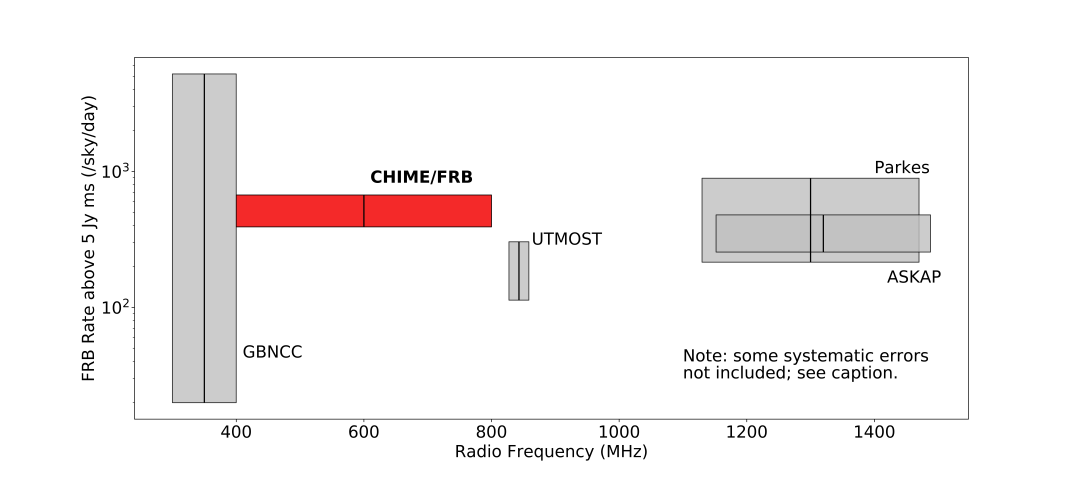
Figure 25: Our new CHIME/FRB rate, along with other recent published rate estimates, all scaled to a fluence limit of 5 Jy ms using our value of $\alpha=-1.41$, Equation 14, and assuming a flat spectral index. Uncertainties on the scaled rate account for uncertainties on the pre-scaled rate and on $\alpha$, including both statistical and systematic values as applicable. We caution, however, that these data, originating from different instruments and processed with different techniques, are not directly comparable. Uncertainties in the frequency distribution, rate versus bandwidth and its evolution with frequency, choice of fluence cutoff, fluence distribution index versus DM, and other effects have not been accounted for in this simple comparison. The apparent discrepancies in measured all-sky rates presented in this figure may fall within the systematic differences arising from these effects.

8 Conclusions

We have presented the largest ever sample of FRBs, increasing the public sample of FRBs by nearly a factor of four. For each burst, we measure detailed pulse properties, including parameters from a pulse-model fit. This provides a large sample of bursts, from both repeating and so-far non-repeating sources, with homogeneous detection pipelines, selection biases, and property measurements.

The sample has also enabled a direct comparison of bursts from repeating sources to bursts from sources that have so far not been observed to repeat. We find that repeaters and apparent non-repeaters show DM, scattering, sky-location, and signal-strength distributions consistent with coming from the same underlying population. However, we confirm distinct differences in both the intrinsic temporal and spectral morphology of the two populations. This may suggest that repeaters and one-off FRBs are distinct populations, or perhaps that repeat rate strongly correlates with morphology.

In addition, we have developed algorithms and techniques for a synthetic signal injection system to forward model the selection biases in the CHIME/FRB system as a function of the burst properties and employed these tools for our analyses. This permits a measurement of FRB property distributions in an absolute sense, revealing a sizeable population of very highly scattered events, only a fraction of which are detected. We have measured the FRB sky rate and fluence distribution, showing that the latter is consistent with the Euclidean expectation when including the full range of observed DMs. However, we find hints of the detailed shape of the FRB energy distribution in the observed joint distribution of fluence and DM.

The rich dataset represented by the CHIME/FRB Catalog 1 will be explored in further detailed studies by our team. The statistics of pulse spectro-temporal morphology, including pulses from both repeating and non-repeating sources, are presented in Pleunis et al. (2021, submitted). The sky distribution of FRBs with respect to the Galactic plane is presented in Josephy el al. (2021, submitted). A cross-correlation analysis of the catalog sources with galaxy catalogs will be presented by Rafiei-Ravandi et al. (in preparation) and a detailed study of the joint distribution of DM and scattering will be performed in Chawla et al. (in preparation). The flux and fluence calibration techniques we use will be presented in detail by Andersen et al. (in preparation), determination of the CHIME beam model will be presented by Singh et al. (in preparation) and Wulf et al. (in preparation), and the injection system we use to characterize selection effects will be presented in Merryfield et al. (in preparation). The details of our use of both the catalog and the injections sample to correct for selection biases and for statistical inference will be presented in Munchmeyer et al. (in preparation). Accompanying these latter two papers will be a public release of the injection sample. Also, we are actively working on analyzing the joint distribution of fluence and DM and interpreting it with respect to the FRB energy distribution function.

We look forward to the broader FRB and astrophysical community making use of the first CHIME/FRB catalog for new interpretations of our results and for purposes we have yet to envision. The release of Catalog 1 also marks the start of public, near real-time alerts of FRB candidates via Virtual Observatory VOEvents, which we hope will enable a myriad of transient FRB follow-up and multi-wavelength science, in a continuing effort to determine the origins of these enigmatic sources.

Appendix A Transient Name Server Names for Fast Radio Bursts

The Transient Name Server (TNS) is a public online archive and alert system for new astrophysical transients that was officially adopted by the IAU as of 2016 January. The CHIME/FRB Collaboration, in consultation with the FRB research community, has selected an FRB naming scheme that is now officially maintained through the TNS and by which all Catalog 1 discoveries are named. For the benefit of the wider FRB community, here we provide instructions for observers to catalog their FRB discoveries through the TNS.

New FRB discoveries can be submitted to the TNS by a human through the use of an online web form submission, or in an automated fashion by a computer program referred to as a bot within the TNS. The first step is to create TNS user accounts for oneself and team members, and subsequently a TNS group account to which said members should be added. Each TNS group is given access to a TNS bot for which a unique API key will be generated and provided by the TNS. The TNS exposes a limited set of archiving functions, allowing the user to submit or retrieve FRB discoveries automatically with a script, through a selection of URL endpoints. The TNS provides official templates for such scripts in select programming languages, including python, and it is here that the user is required to plug in their API key.

A minimal set of measurements and identifiers must be provided with every FRB discovery to be accepted by the TNS. These include Right Ascension, Declination, the discovery date and time (topocentric) of the event, the DM, the instrument or observatory, the reference frequency of the burst, the instrument bandwidth, the number of frequency channels, and the sampling time (among other administrative details). Further information can be provided including a machine-readable list of vertices for an elliptical or polygonal sky localization region. Virtually any supporting file type (e.g., a PNG file for the burst dynamic spectrum in the observing band) can be uploaded as supporting evidence.

FRBs are submitted through the TNS API in bulk discovery reports formatted as JSON documents. The default script for accessing the TNS API returns either the TNS object name for each new FRB object that was added, or a list of error messages (one per offending discovery entry) in the event that the submission data were incomplete or malformed. Under normal conditions, the TNS API updates their database within $\sim 1~{}\text{s}$ per bulk submission, though it is considered good practice to verify automated submissions after allowing enough time for the updating to finish. New TNS users should exercise caution during bulk submission: if a single FRB within the bulk report is rejected by the TNS, all discoveries in the report are rejected. Therefore, validation of the discovery data before submission, and of the TNS response submission, is an essential component of any system designed to submit in real-time to the TNS.

New TNS users are strongly encouraged to practice their FRB submissions using the TNS sandbox site before proceeding to the live site. Just as with the live site, the sandbox site offer TNS users the option to specify the end date and time of a proprietary period during which their new FRB submissions are not visible outside their TNS group. This can be leveraged for users to practice internal bookkeeping with official TNS names, without exposing their discoveries publicly at least for some time.

Appendix B Quality of least-squares fits to burst morphology models

Here we provide additional details on the least-squares fitting procedure as implemented in fitburst. We define the noise-weighted fit residuals to be

$$h_{t,f}(\boldsymbol{\lambda})=\frac{d_{t,f}}{\sigma_{f}}-S_{t,f}(\boldsymbol{\lambda}),$$ (B1)

where $d_{t,f}$ is the total intensity data as a function of discrete time $t$ and discrete frequency $f$ (the dynamic spectra), $S_{t,f}$ is the model defined as a function of the parameter vector $\boldsymbol{\lambda}$ as described in Section 3.3, and $\sigma_{f}$ is the noise standard deviation measured in each spectral channel. Note that $S_{t,f}(\boldsymbol{\lambda})$ is not divided by ${\sigma_{f}}$ in the above equation, meaning that for the morphology fits we are effectively calibrating the data to uniform noise, a choice we have found to yield the most robust results if not trying to extract absolute flux information (which is measured elsewhere). Prior to fitting the data are detrended with a temporal high-pass filter and cleaned with an automatic narrowband RFI-detection algorithm that excises spectral channels based on variance and spectral-kurtosis distributions. Using the optimize.least_squares solver provided by the open-source scipy software library (Virtanen et al., 2020), fitburst minimizes $\chi^{2}(\boldsymbol{\lambda})=\sum_{t,f}[h_{t,f}(\boldsymbol{\lambda})]^{2}$ with respect to the parameters.

In addition to best-fit parameters, we tabulate in Catalog 1 several metrics to help assess the quality of these fits. The first is the fraction of spectral channels that are missing or flagged as RFI. Second, the fitburst SNR equal to $\sqrt{\Delta\chi^{2}}$, where $\Delta\chi^{2}$ is the difference in $\chi^{2}$ between the best fit model and the no-burst model ($S_{t,f}=0$). We also provide the best fit value of $\chi^{2}$ as well as the number of degrees of freedom for the fit, allowing the reduced chi-square statistic to be calculated and chi-squared tests to be performed. Finally, for each burst we provide waterfall plots of the noise-weighted fit residuals in Figures 26 and 27 such that the quality of the fit for each burst may be assessed visually.

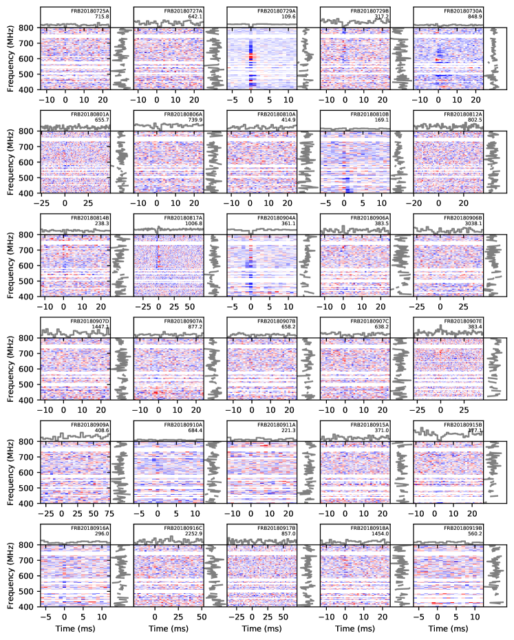
Figure 26: Waterfall plots of fitburst residuals, down-sampled in frequency, for one-off bursts. Same as Figure 7 except showing the normalized residuals from the best-fit model. Color scale saturates at $\pm 3\sigma$. Panels for all catalog one-off bursts can be found at https://www.canfar.net/storage/list/AstroDataCitationDOI/CISTI.CANFAR/21.0007/data/additional_figures/residuals.

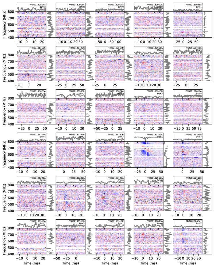
Figure 27: Waterfall plots of fitburst residuals for repeaters. Same as Figure 26 except for repeaters (as in Figure 8). Panels for all catalog repeating bursts can be found at https://www.canfar.net/storage/list/AstroDataCitationDOI/CISTI.CANFAR/21.0007/data/additional_figures/residuals.

As can be seen in the residual plots, the temporal profiles are usually well modeled with intrinsic or scatter-broadened Gaussian shapes. Remaining residual structure tends to be most prominent along the frequency axis. These features indicate that a smooth, running power-law spectrum is an imperfect model for many events. Indeed, Macquart et al. (2019) analyzed 23 dynamic spectra observed with ASKAP and argued that the diversity in their measurements arises from effects intrinsic to FRB emission and/or propagation, such as diffractive scintillation. Moreover, the telescope beam and non-uniformity in the noise levels as a function of spectral frequency can introduce spectral structure for which we have not accounted. We nonetheless used the running power-law spectral model in our modeling of all CHIME/FRB events for uniformity in our analysis and interpretation. Further analysis of fluctuations in total intensity across the CHIME band will be reserved for future work.

In some cases, structure in the residuals is the result of poorly modeled temporal profiles or failures of the least-squares solver to converge to an adequate result, both of which are subject to human interaction and judgement. For example, a number of components ($n$ in Section 3.3) greater than unity were visually determined; it is likely that faint bursts with marginally complex morphology were instead modeled as single-component bursts, which would impact best-fit estimates of several fit parameters described above. Similarly, even single component bursts may not be well modelled by an intrinsically Gaussian pulse profile multiplied by a generalized power law. Moreover, the least-squares algorithm may yield sub-optimal estimates of parameter estimates and uncertainties that could instead be sampled better using the Markov Chain Monte Carlo (MCMC) method. Various efforts for improving the automated fitting pipeline, including the use of an MCMC sampler for fitburst and an automatic determination of the number of components, are ongoing and will be the subject of future CHIME/FRB catalogs.

Interpretations of the burst properties in Catalog 1 should thus be taken in the context of these limitations. At the population level, there may be significant biases in the measured properties (e.g., biases in the spectral index due to the beam, as shown in Figure 20). For individual bursts, the quality of a given fit should be accessed through $\chi^{2}$ statistics and the residual plots. Nonetheless, if proper care is taken to determine the impact of these issues, the data presented here are adequate for a wide range of analyses including those presented in this article and in companion works.

Appendix C Fitting for a fiducial population model

Here we detail the procedure for finding a fiducial model for the property distributions $P(F)$, $P(\mathrm{DM})$, $P(\tau)$, $P(w)$, and $P(\gamma,r)$, as introduced in Section 6. The purpose of the fiducial model is not to provide a precise description of the true property distributions, but a rough one, such that correlated selection effects are accounted for when performing deeper analyses in property subspaces.

C.1 Property distribution models and overview of fitting procedure

Empirically, we found that the following models for the intrinsic property distribution functions $P(\xi)$ provide a reasonable match to the data:

• Fluence is described by a power-law distribution $P(F)\propto-\alpha(F/F_{0})^{\alpha-1}$ with power-law index $\alpha$.

• DM, scattering $\tau$, and pulse width $w$ are described by log-normal distributions with a shape $\sigma$ and scale $m$, given by $P(\xi)=\frac{1}{\sigma(\xi/m)\sqrt{2\pi}}\exp\left[-\frac{\ln^{2}{(\xi/m)}}{2\sigma^{2}}\right]$.

• For the spectral index $\gamma$ and running $r$, we fit a kernel density estimator to their joint observed distribution and equate it to the intrinsic distribution without compensating for selection effects. However, we do verify that, once accounting for measurement effects from the beam, the final population model provides a reasonable description of the catalog data (see Figure 20).

Rather than performing a joint fit to the parameters of all property distributions simultaneously, we use an iterative fitting scheme, where we optimize the parameters of each population factor $P(\xi)$ independently while keeping the other parameters fixed. This method is possible because of our assumption that the rate function factorizes, and is necessary because of our limited injections sample—we do not have enough injections to fully determine the 7D observation function $P(\mathrm{SNR}|F,\mathrm{DM},\tau,w,\gamma,r)$; however, we can determine certain integrals thereof. We are currently exploring the use of machine learning to fully determine the observation function.

Schematically, our fitting procedure is as follows:

1. On the $i=0$ iteration, define an initial model $R_{i=0}=R_{{\rm init}}$ for the intrinsic rate composed of individual property distribution models $P_{i=0}=P_{{\rm init}}$.

2. On each iteration $i$, and for each property $\xi$ in $(F,\mathrm{DM},\tau,w)$, form the selection function $s_{i}(\xi)=P_{{\rm obs},i}(\xi)/P_{i}(\xi)$, obtaining the observed distribution from the injection system.

3. Fit a model $P_{\rm obs}(\xi)=s_{i}(\xi)P_{i+1}(\xi)$ to the catalog data.

4. Iterate steps 2 and 3 until convergence. The converged result is the fiducial model.

C.2 Modeling observed population with injections

The initial probability density functions $P_{\rm init}(\xi)$ are the same as those used for the injections population described in Section 4.1.2 and are designed to both fully sample the range of observed properties and more densely sample parts of phase space populated by the catalog. We take care to apply the same cuts to the injected events as we did to the catalog, including automated RFI classification, and cuts on galactic DM. Less than half of the 84 697 detected injections survive these cuts, with most of the attrition coming from the $\mathrm{SNR}>12$ requirement for population analysis. These cuts provide a sample of $\mathcal{R}_{\rm obs,init}(\mathrm{SNR},\mathrm{DM},\tau,w,\gamma,r)$. The sample is not dense enough to fully determine this 7D function; however, integrals thereof such as $P_{\rm obs,init}(\mathrm{DM})$ are determined with little sampling noise.

At each iteration $i$ of our fitting procedure described above, a simple approach would be to generate a new population $R_{i}$ of FRBs from the best-fit parameters at the current iteration, inject these into the pipeline, and thus obtain a new observed distribution $\mathcal{R}_{\mathrm{obs},i}$. However, we can avoid re-running the injections system at each iteration; using the initial injected population, we can generate populations for any new distribution as follows.

Our injections sample was drawn from $R_{\rm init}(F,\mathrm{DM},\tau,w,\gamma,r)$, providing corresponding samples of $\mathcal{R}_{\rm obs,init}(\mathrm{SNR},\mathrm{DM},\tau,w,\gamma,r)$ after injection. These can be converted to estimates of $P_{\rm init}(\xi)$ and $P_{\rm obs,init}(\xi)$ by accumulating these samples from the full and detected injections into histograms respectively. Further, this can be converted to any new model $R(F,\mathrm{DM},\tau,w,\gamma,r)$ by reweighting the sample—for every event, we construct weights

$$W(F,\mathrm{DM},\tau,w,\gamma,r)=\frac{R(F,\mathrm{DM},\tau,w,\gamma,r)}{R_{\rm init}(F,\mathrm{DM},\tau,w,\gamma,r)}.$$ (C1)

Accumulating the FRB injection sample into histograms, counting each event with weight $W$ then provides estimates of $P(\xi)$ (for the full injection sample), and $P_{\rm obs}(\xi)$ (for the detected events) for the new model rather than the initial model. $P_{\rm obs}(\xi)$ is thus our prediction for the catalog, to which we fit the underlying parameters by optimizing a likelihood analogous to Equation 13 (holding the distributions of properties other than $\xi$ fixed on a given iteration).

C.3 Jackknife tests

Jackknife tests provide a way to search for inconsistencies in the data by splitting the sample by some criteria and comparing the changes in the analysis results to those expected statistically from the cut. A full study of the uncertainty in the fiducial model (either statistical or systematic) is beyond the scope of this work, since it is only used as a starting point for further analysis. However, we can use our procedure for finding the fiducial model to search for systematic errors, as well as test our strongest assumption: that the FRB properties are intrinsically uncorrelated. We note that we do perform an accounting of uncertainties for our final $\alpha$ and sky-rate measurements in Section D, much of which is informed by the jackknife tests presented here.

We perform the following jackknife tests:

• A set of 50 “random” jackknives, where half the 265 events in the post-cut sample are excluded at random to give an indication of the expected change in parameters from the smaller sample size. For each parameter we quote the mean and standard deviation (SD) over the set.

• Shifting the SNR cut from 12 to either 10 or 14 to check for incompleteness in the human classification step of catalog events. This would not be accounted for by the injections, since detected injections are verified by coincidence with an input injection, rather than human classification.

• Separate cuts on DM, $w$, and $\tau$ near the median values of the sample. These cuts test for intrinsic correlations among properties in the sample. When cutting on a given property, e.g., $\tau$, we fix the model $P(\tau)$ at the fiducial model. This better tests for correlations in the properties, rather than how the reduced data range for a given property affects the fit.

The results of the iterative model fitting for these jackknives are quoted in Table 4.

Table 4: Best Fit Parameters for Full Sample and Jackknife Subsamples

Parameter	Fiducial (full)	Random (SD)	Random (mean)	SNR $>10$	SNR $>14$	DM $>500^{\rm a}$	$w$ $<1$ ms	$\tau$ $<1$ ms
Nevents	265	…	$-133$	94	$-48$	$-118$	$-97$	$-130$
$\alpha$	$-1.32$	0.11	$-0.01$	$-0.09$	$-0.1$	$-0.35$	0.14	0.33
DM scale / $100^{\rm a}$	4.95	0.22	0.02	0.17	$-0.05$	…	$-0.37$	$-0.91$
DM shape	0.66	0.03	$-0.01$	0.02	0.01	…	0.01	$-0.02$
$w$ scale (ms)	1.0	0.08	$-0.02$	0.19	$-0.13$	0.2	…	$-0.43$
$w$ shape	0.97	0.08	$-0.01$	0.02	$-0.06$	0.06	…	$-0.32$
$\tau$ scale (ms)	2.02	1.31	0.31	0.02	0.24	1.11	0.14	…
$\tau$ shape	1.72	0.26	0.02	$-0.15$	0.08	$-0.14$	0.75	…

Notes. Results of the iterative model fitting procedure for the full sample (yielding our fiducial model) and jackknife samples. The fitting procedure and parameter definitions are described in Appendix C.1. When cutting on DM, $w$, or $\tau$, we fix the model parameters for that property’s distribution at the fiducial values. Values to the right of the vertical line are differences from the fiducial values.
^a DMs are in units of pc cm^-3

Some caution is required in interpreting the standard deviation of the random jackknives in terms of the expected shift in parameter values. For the SNR cuts, much less than half the sample is excluded or added, and the fit lever arm for $\alpha$ also changes. When cutting on DM, $w$, and $\tau$, roughly half the sample is cut. However, the cut events have weights that are systematically different from a typical event, especially for $\tau$ where the cut events are upweighted by the fitting procedure because of the low selection function. A precise accounting for the expected statistical fluctuation in each jackknife is beyond the scope of this paper. The standard deviation of the random jackknives nonetheless gives a rough sense for how much we expect parameters to vary, and the tests are valuable to search for strong biases and strong property correlations of the type that might invalidate conclusions drawn from our analysis.

While the results of our jackknife tests do allow for order-unity property correlations, we do not find evidence for very strong systematic errors or property correlations (i.e., above 90%).

Shifting the SNR cut does produce a shift in $\alpha$ of $\sim 0.1$, which is larger than one might expect given the modest change in event numbers. This may be an indication of residual bias from human classification, although this explanation is at odds with the fact that the shift in $\alpha$ is in the same direction when either raising or lowering the threshold. There would also seem to be a significant change in the width scale parameter. This might indicate a negative correlation between fluence (which is correlated with SNR) and width, although we find this to be physically implausible. Another explanation is that this is a measurement effect, with narrow widths difficult to measure to low SNR events, yielding upper limits that may be significantly higher than their true values. We note that our analysis fully compensates for completeness as a function of properties such as $w$, but not in errors in the measurement of the properties themselves.

Jackknives in DM, $w$, or $\tau$ all result in changes in the $\alpha$ parameters. For DM, this change in $\alpha$ is studied in detail in Section 6.2. The shift for the $w$ jackknife is not particularly significant compared to the random jackknives. Interpreting the shift for the $\tau$ jackknife is complicated by the highly non-uniform weighting of events as a function of $\tau$, making the expected statistical fluctuation difficult to calculate.

These jackknives also result in shifts in the DM, $w$, or $\tau$ scale parameters consistent with order-unity correlations between these properties. In particular, we see hints of a positive DM–$\tau$ correlation, both from the change in DM scale in the $\tau$ jackknife and the change in the $\tau$ scale in the DM jackknife. Such a correlation is well motivated physically and will be studied in detail in future work. Likewise, there is evidence for a $w$–$\tau$ correlation, although this is likely a measurement effect since these properties are particularly hard to disentangle observationally.

Appendix D Systematic errors in the rate and $\alpha$ measurement

There are several sources of systematic errors in our measurements. Obtaining the sky rate requires an absolute accounting of the survey duration $\Delta t$. As described in Section 2.2, our effective survey duration is 214.8 days. Note that periods where the system was operating well below nominal sensitivity have been excluded from this figure and any bursts discovered during these periods have been excluded from the population analysis.

Nonetheless, our measurement of the overall rate depends on the sensitivity during the injections campaign (which occurred in August 2020) being representative of the full Catalog 1 period. Between the beginning of the survey and the injections campaign, we estimate our noise levels have improved by 6%, based on daily observations of the SNRs of pulsar single-pulse detections. The change since the midpoint of the survey period was 3%. To compensate for this, we reduce our effective survey duration by $|\alpha|\times 3\%$, using $\alpha=-3/2$ which is the value for a stationary universe and is consistent with our measurement in Section 6.2. We allow for a corresponding systematic error in our rate measurement of $|\alpha|\times 3\%=4.5\%$.

Another source of systematic error in the rate is incompleteness in Catalog 1 not accounted for by injections. Injected events are only processed by our automated pipeline, and lack a final human classification step required for true events. However, our human classification should be complete above an L1 SNR of 12. There are 28 cases where an FRB candidate was successfully classified by the automated pipeline, but due to a system error no intensity data were saved. Of these 16 events would have passed our cuts on SNR and occurred during periods where the system was otherwise operating nominally. For such events, we have no way of knowing whether they would have survived human classification or our other various data cuts. This leads to an additional, one-sided systematic error in the rate of $+16/265=+6.0\%$.

A large source of uncertainty in our analysis is the telescope beam. The CHIME beam model used for injections is described in Section 4. This model was verified by comparing to measurements of the Sun over the declination range $\pm 23.4$ degrees, as well as holographic measurements of bright persistent sources for a few specific declinations (see Section 2.1). The discrepancy between these measurements and our primary beam model, in units of the peak power response at the declination of Cygnus A, is of order 0.1 in the main lobe and 0.01 in the near side lobes. These discrepancies vary in magnitude and sign as a function of both frequency and declination. As such, we expect a high degree of cancellation in averages over frequencies and beams. Nonetheless, to conservatively account for errors in the main-lobe response, we assign a systematic uncertainty in our rate measurement of $|\alpha|\times 10\%=15\%$. We are insensitive to beam-model errors in the side lobes since we are able to identify side-lobe FRB detections from their spectral characteristics and have cut them from our analysis. However, some possibility of side-lobe contamination from narrow band bursts does exist.

In our $\alpha$ measurement, we do not account for systematic error from the beam, which should be small because our analysis uses $\mathrm{SNR}$ as our observable rather than fluence directly. It has been shown that the $\mathrm{SNR}$ distribution power law index is unaffected by the telescope beam (Oppermann et al., 2016; Connor, 2019; James et al., 2019), provided FRB fluences are distributed as a single power law, the instrumental $\mathrm{SNR}$ is linear in the FRB fluence, and chromatic effects are ignored. All three of these assumptions are violated, however, we account for these in our primary analysis, relying on them only at the level of the beam-model uncertainty. The effect on our $\alpha$ measurement is thus second order (an error on an error) and can be neglected.

To avoid a high-dimensional fitting problem and to make best use of our finite injection sample, we have opted to study FRBs in the property space of fluence and DM, fixing the other properties at their fiducial distributions. This treatment can induce errors that are not accounted for in the statistical uncertainty in two ways. First, even if our model without intrinsic correlations were correct, not fitting simultaneously means we neglect correlated statistical errors in the distribution parameters. For instance, a 1$\sigma$ fluctuation in the scattering scale parameter would shift the scattering distribution to a region with more or less selection bias, resulting in a different inferred overall rate. Second, our model where the FRB properties are intrinsically uncorrelated could be incorrect. Indeed, Table 4 contains evidence for correlations amongst fluence, DM, width, and scattering. As an estimate for how large these errors could be, we perturb the scale parameters for both width and scattering. For the scattering scale, we perturb by $\pm 1$ ms and for the width scale by $\pm 0.3$ ms, inspired by the magnitude of deviation we see in Table 4. The perturbation in scattering scale has the larger effect, resulting in changes in $\alpha$ of $\pm 0.03$ and in the overall rate of ${}^{+18\%}_{-20\%}$. This treatment conservatively captures the issue of correlations in the parameter fits; however, we caution that the effects of intrinsic property correlations could be more subtle and will need to be studied further. In addition, our only treatment of the spectral properties $\gamma$ and $r$ is to show that the distribution of the observed injections population roughly matches that of Catalog 1, a treatment that is far from complete.

As previously discussed, another concern is incompleteness in Catalog 1 from human classification that is not reflected in the injections. Shifting our SNR cut from 12 to 16 changes $\alpha$ by $-0.08$ and the rate by $+10\%$. While these changes are largely within the expectation for statistical fluctuations from the number of cut events, they are in the direction one would expect for residual incompleteness at low SNR. We thus conservatively include these figures in our systematic error budget.

Prior to the addition of the RFI classification bypass for high-SNR events described in Section 2, there were three events with $\mathrm{SNR}\gtrsim 100$ that were likely to have been astrophysical but are not included in Catalog 1 as they were classified as RFI, and thus their data were not retained. Including these events in the population analysis shifts $\alpha$ by $+0.05$ (which we include in our error budget) but has a negligible effect on the rate.

During the Catalog 1 period and between then and the injections period, there have been a number of other changes to our detection pipeline, including changes to the RFI cleaning and the addition of automated classifiers employing machine learning. In addition, there have been changes in the RFI environment at the telescope site. While these changes are difficult to quantify, they should be an overall small effect above our relatively high SNR cutoff for statistical analysis of 12. The assessment of the effect of changing the SNR cutoff in the previous paragraph also partially accounts for this effect as does our tracking of the overall telescope sensitivity using pulsar pulses.

All systematic errors are added in quadrature. For the rate, this yields a net systematic error of ${}^{+27\%}_{-25\%}$. For $\alpha$ the systematic error is ${}^{+0.060}_{-0.085}$.

Appendix E Catalog excerpt

In Table 5, we provide an excerpt from Catalog 1. We show all fields for four Catalog 1 entries. The first entry is a so-far non-repeating source detected during the pre-commissioning period, the second entry is another so-far non-repeating source, and the latter two are sub-bursts from the same event from a repeating FRB. Field descriptions can be found in Table LABEL:ta:catalog and the full Catalog 1 data accompanies the online version of this article and at the CHIME/FRB Public Webpage.

Table 5: Excerpt from Catalog 1

tns_name	previous_name	repeater_name	ra	ra_err	ra_notes	dec	dec_err
			(degrees)	(degrees)		(degrees)	(degrees)
FRB20180817A	180817.J1533+42	…	233.200	0.052	…	42.20	$0.16$
FRB20180915B	…	…	225.23	0.25	…	25.02	$0.23$
FRB20180917A	…	FRB20180814A	65.54	0.19	…	73.63	$0.27$
FRB20180917A	…	FRB20180814A	65.54	0.19	…	73.63	$0.27$

dec_notes	gl	gb	exp_up	exp_up_err	exp_up_notes	exp_low	exp_low_err
	(degrees)	(degrees)	(hours)	(hours)		(hours)	(hours)
…	$68.3$	$53.98$	$22.7$	$2.5$	…	…	…
…	$36.17$	$60.93$	$13.1$	$7.6$	…	…	…
…	$136.46$	$16.58$	$41$	$24$	…	$43.5$	$7.9$
…	$136.46$	$16.58$	$41$	$24$	…	$43.5$	$7.9$

exp_low_notes	bonsai_snr	bonsai_dm	low_ft_68	up_ft_68	low_ft_95	up_ft_95	snr_fitb
		(pc cm-3)	(Jy ms)	(Jy ms)	(Jy ms)	(Jy ms)
…	$45.6$	$1002.8$	$0$	$6.2$	$0$	$11.1$	$65.1$
…	$12.5$	$176.3$	$0$	$2.4$	$0$	$4.2$	$36.1$
…	$19$	$194.1$	$43.8$	$6.9$	$155.9$	$25.6$	$46.6$
…	$19$	$194.1$	$43.8$	$6.9$	$155.9$	$25.6$	$46.6$

dm_fitb	dm_fitb_err	dm_exc_ne2001	dm_exc_ymw16	bc_width	scat_time	scat_time_err	flux
(pc cm-3)	(pc cm-3)	(pc cm-3)	(pc cm-3)	(s)	(s)	(s)	(Jy)
1006.7714	$0.0085$	$979.1$	$982.0$	0.01769	$0.01103$	$0.00058$	$2.4$
177.127	$0.020$	$154.7$	$154.1$	0.00492	$0.0001108$	$0.0000081$	$0.99$
189.917	$0.018$	$102.1$	$81.5$	0.06095	$0.0080$	$0.0025$	$3.2$
189.917	$0.018$	$102.1$	$81.5$	0.06095	$0.0080$	$0.0025$	$3.2$

flux_err	flux_notes	fluence	fluence_err	fluence_notes	sub_num	mjd_400	mjd_400_err
(Jy)		(Jy ms)	(Jy ms)			(MJD)	(MJD)
$1.5$	…	$29$	$16$	…	$0$	$58347.0760879598$	$0.0000000031$
$0.42$	…	$3.8$	$1.0$	…	$0$	$58376.9753845892$	$0.0000000021$
$3.1$	…	$46$	$32$	…	$0$	$58378.0323858329$	$0.0000000068$
$3.1$	…	$46$	$32$	…	$1$	$58378.0323860277$	$0.0000000097$

mjd_inf	mjd_inf_err	width_fitb	width_fitb_err	sp_idx	sp_idx_err	sp_run
(MJD)	(MJD)	(s)	(s)
$58347.0757860647$	$0.0000000040$	$0.00189$	0.00017	$3.35$	$0.40$	$-7.46$
$58376.9753314751$	$0.0000000063$	$0.001694$	0.000075	$-9.2$	$1.0$	$3.0$
$58378.0323288836$	$0.0000000088$	$0.00178$	0.00026	$34$	$18$	$-19$
$58378.032329078$	$0.000000011$	$0.00345$	0.00044	$52.3$	$7.7$	$-46.5$

sp_run_err	high_freq	low_freq	chi_sq	dof	flag_frac	peak_freq	excluded_flag
	(MHz)	(MHz)				(MHz)
$0.56$	$800.2$	$400.2$	$1069085.403$	$1057913$	$0.434$	$501.1$	$1$
$2.8$	$527.4$	$400.2$	$278172.462$	$276025$	$0.557$	$400.2$	$0$
$14$	$800.2$	$658.6$	$908712.749$	$904687$	$0.516$	$800.2$	$0$
$6.8$	$800.2$	$561.8$	$908712.749$	$904687$	$0.516$	$701.7$	$0$

References

- Agarwal et al. (2020) Agarwal, D., Lorimer, D. R., Surnis, M. P., et al. 2020, MNRAS, 497, 352, doi: 10.1093/mnras/staa1927
- Amiri et al. (2017) Amiri, M., Bandura, K., Berger, P., et al. 2017, ApJ, 844, 161, doi: 10.3847/1538-4357/aa713f
- Bandura et al. (2016) Bandura, K., Bender, A. N., Cliche, J. F., et al. 2016, Journal of Astronomical Instrumentation, 5, 1641005. https://arxiv.org/abs/1608.06262
- Beloborodov (2017) Beloborodov, A. M. 2017, ApJ, 843, L26, doi: 10.3847/2041-8213/aa78f3
- Beloborodov (2020) —. 2020, arXiv e-prints, arXiv:2011.07310. https://arxiv.org/abs/2011.07310
- Beniamini et al. (2021) Beniamini, P., Kumar, P., Ma, X., & Quataert, E. 2021, MNRAS, 502, 5134, doi: 10.1093/mnras/stab309
- Berger et al. (2016) Berger, P., Newburgh, L. B., Amiri, M., et al. 2016, 9906, 99060D, doi: 10.1117/12.2233782
- Bhandari et al. (2018) Bhandari, S., Keane, E. F., Barr, E. D., et al. 2018, MNRAS, 475, 1427, doi: 10.1093/mnras/stx3074
- Bhandari et al. (2020) Bhandari, S., Sadler, E. M., Prochaska, J. X., et al. 2020, ApJ, 895, L37, doi: 10.3847/2041-8213/ab672e
- Bochenek et al. (2020) Bochenek, C., Kulkarni, S., Ravi, V., et al. 2020, The Astronomer’s Telegram, 13684, 1
- Burke-Spolaor & Bannister (2014) Burke-Spolaor, S., & Bannister, K. W. 2014, ApJ, 792, 19, doi: 10.1088/0004-637X/792/1/19
- Champion et al. (2016) Champion, D. J., Petroff, E., Kramer, M., et al. 2016, MNRAS, 460, L30, doi: 10.1093/mnrasl/slw069
- Chatterjee et al. (2017) Chatterjee, S., Law, C. J., Wharton, R. S., et al. 2017, Nature, 541, 58. https://arxiv.org/abs/1701.01098
- Chawla et al. (2017) Chawla, P., Kaspi, V. M., Josephy, A., et al. 2017, ApJ, 844, 140. https://arxiv.org/abs/1701.07457
- CHIME/FRB Collaboration et al. (2018) CHIME/FRB Collaboration, Amiri, M., Bandura, K., et al. 2018, ApJ, 863, 48, doi: 10.3847/1538-4357/aad188
- CHIME/FRB Collaboration et al. (2019a) CHIME/FRB Collaboration, Andersen, B. C., Bandura, K., et al. 2019a, ApJ, 885, L24, doi: 10.3847/2041-8213/ab4a80
- CHIME/FRB Collaboration et al. (2019b) CHIME/FRB Collaboration, Amiri, M., Bandura, K., et al. 2019b, Nature, 566, 230, doi: 10.1038/s41586-018-0867-7
- CHIME/FRB Collaboration et al. (2019c) —. 2019c, Nature, 566, 235, doi: 10.1038/s41586-018-0864-x
- CHIME/FRB Collaboration et al. (2020a) CHIME/FRB Collaboration, Amiri, M., Andersen, B. C., et al. 2020a, Nature, 582, 351, doi: 10.1038/s41586-020-2398-2
- CHIME/FRB Collaboration et al. (2020b) CHIME/FRB Collaboration, Andersen, B. C., Bandura, K. M., et al. 2020b, Nature, 587, 54, doi: 10.1038/s41586-020-2863-y
- Connor (2019) Connor, L. 2019, MNRAS, 487, 5753, doi: 10.1093/mnras/stz1666
- Connor et al. (2020) Connor, L., Miller, M. C., & Gardenier, D. W. 2020, MNRAS, 497, 3076, doi: 10.1093/mnras/staa2074
- Cordes & Chatterjee (2019) Cordes, J. M., & Chatterjee, S. 2019, ARA&A, 57, 417, doi: 10.1146/annurev-astro-091918-104501
- Cordes & Lazio (2002) Cordes, J. M., & Lazio, T. J. W. 2002
- Cordes et al. (2017) Cordes, J. M., Wasserman, I., Hessels, J. W. T., et al. 2017, ApJ, 842, 35. https://arxiv.org/abs/1703.06580
- Crawford et al. (2016) Crawford, F., Rane, A., Tran, L., et al. 2016, MNRAS, 460, 3370, doi: 10.1093/mnras/stw1233
- Farah et al. (2019) Farah, W., Flynn, C., Bailes, M., et al. 2019, MNRAS, 488, 2989, doi: 10.1093/mnras/stz1748
- Fasano & Franceschini (1987) Fasano, G., & Franceschini, A. 1987, MNRAS, 225, 155, doi: 10.1093/mnras/225.1.155
- Fonseca et al. (2020) Fonseca, E., Andersen, B. C., Bhardwaj, M., et al. 2020, ApJ, 891, L6, doi: 10.3847/2041-8213/ab7208
- Foreman-Mackey et al. (2013) Foreman-Mackey, D., Hogg, D. W., Lang, D., & Goodman, J. 2013, PASP, 125, 306, doi: 10.1086/670067
- Gehan (1965) Gehan, E. A. 1965, Biometrika, 52, 203
- Gupta et al. (2021) Gupta, V., Flynn, C., Farah, W., et al. 2021, MNRAS, 501, 2316, doi: 10.1093/mnras/staa3683
- Harrington & Fleming (1982) Harrington, D. P., & Fleming, T. R. 1982, Biometrika, 69, 553, doi: 10.1093/biomet/69.3.553
- Hashimoto et al. (2020) Hashimoto, T., Goto, T., On, A. Y. L., et al. 2020, MNRAS, 497, 4107, doi: 10.1093/mnras/staa2238
- Helsel (2005) Helsel, D. R. 2005, Nondetects and data analysis. Statistics for censored environmental data. (Wiley-Interscience)
- Herschel (1785) Herschel, W. 1785, Philosophical Transactions of the Royal Society of London Series I, 75, 213
- Ioka & Zhang (2020) Ioka, K., & Zhang, B. 2020, ApJ, 893, L26, doi: 10.3847/2041-8213/ab83fb
- James et al. (2019) James, C. W., Ekers, R. D., Macquart, J. P., Bannister, K. W., & Shannon, R. M. 2019, MNRAS, 483, 1342, doi: 10.1093/mnras/sty3031
- James et al. (2021a) James, C. W., Prochaska, J. X., Macquart, J. P., et al. 2021a, arXiv e-prints, arXiv:2101.07998. https://arxiv.org/abs/2101.07998
- James et al. (2021b) —. 2021b, arXiv e-prints, arXiv:2101.08005. https://arxiv.org/abs/2101.08005
- James et al. (2020) James, C. W., Osłowski, S., Flynn, C., et al. 2020, MNRAS, 495, 2416, doi: 10.1093/mnras/staa1361
- Josephy et al. (2019) Josephy, A., Chawla, P., Fonseca, E., et al. 2019, ApJ, 882, L18, doi: 10.3847/2041-8213/ab2c00
- Kahler (1992) Kahler, S. W. 1992, ARA&A, 30, 113, doi: 10.1146/annurev.aa.30.090192.000553
- Karastergiou et al. (2015) Karastergiou, A., Chennamangalam, J., Armour, W., et al. 2015, MNRAS, 452, 1254, doi: 10.1093/mnras/stv1306
- Kaspi (2010) Kaspi, V. M. 2010, Proceedings of the National Academy of Science, 107, 7147, doi: 10.1073/pnas.1000812107
- Keane & Petroff (2015) Keane, E. F., & Petroff, E. 2015, MNRAS, 447, 2852, doi: 10.1093/mnras/stu2650
- Lang (1971) Lang, K. R. 1971, 164, 249
- Lawrence et al. (2017) Lawrence, E., Vander Wiel, S., Law, C., Burke Spolaor, S., & Bower, G. C. 2017, AJ, 154, 117, doi: 10.3847/1538-3881/aa844e
- Lopaka (2020) Lopaka, L. 2020, NADA: Nondetects and Data Analysis for Environmental Data. https://CRAN.R-project.org/package=NADA
- Lorimer et al. (2007) Lorimer, D. R., Bailes, M., McLaughlin, M. A., Narkevic, D. J., & Crawford, F. 2007, Science, 318, 777. https://arxiv.org/abs/0709.4301
- Lorimer & Kramer (2012) Lorimer, D. R., & Kramer, M. 2012, Handbook of Pulsar Astronomy
- Lorimer, D. R. and Kramer, M. (2005) Lorimer, D. R. and Kramer, M. 2005, Handbook of Pulsar Astronomy (Cambridge University Press)
- Lu & Piro (2019) Lu, W., & Piro, A. L. 2019, ApJ, 883, 40, doi: 10.3847/1538-4357/ab3796
- Lyutikov et al. (2020) Lyutikov, M., Barkov, M. V., & Giannios, D. 2020, ApJ, 893, L39, doi: 10.3847/2041-8213/ab87a4
- Macquart & Johnston (2015) Macquart, J.-P., & Johnston, S. 2015, MNRAS, 451, 3278, doi: 10.1093/mnras/stv1184
- Macquart et al. (2019) Macquart, J.-P., Shannon, R. M., Bannister, K. W., et al. 2019, ApJ, 872, L19, doi: 10.3847/2041-8213/ab03d6
- Macquart et al. (2020) Macquart, J. P., Prochaska, J. X., McQuinn, M., et al. 2020, Nature, 581, 391, doi: 10.1038/s41586-020-2300-2
- Manchester & Taylor (1977) Manchester, R. N., & Taylor, J. H. 1977, Pulsars (San Francisco: Freeman)
- Marcote et al. (2020) Marcote, B., Nimmo, K., Hessels, J. W. T., et al. 2020, Nature, 577, 190, doi: 10.1038/s41586-019-1866-z
- Margalit & Metzger (2018) Margalit, B., & Metzger, B. D. 2018, ApJ, 868, L4, doi: 10.3847/2041-8213/aaedad
- Masui et al. (2015) Masui, K., Lin, H.-H., Sievers, J., et al. 2015, Nature, 528, 523. https://arxiv.org/abs/1512.00529
- Masui et al. (2019) Masui, K. W., Shaw, J. R., Ng, C., et al. 2019, ApJ, 879, 16, doi: 10.3847/1538-4357/ab229e
- Masui & Sigurdson (2015) Masui, K. W., & Sigurdson, K. 2015, Phys. Rev. Lett., 115, 121301, doi: 10.1103/PhysRevLett.115.121301
- McKinnon (2014) McKinnon, M. M. 2014, PASP, 126, 476, doi: 10.1086/676975
- Michilli et al. (2021) Michilli, D., Masui, K. W., Mckinven, R., et al. 2021, ApJ, 910, 147, doi: 10.3847/1538-4357/abe626
- Ng et al. (2017) Ng, C., Vanderlinde, K., Paradise, A., et al. 2017, in Proceedings of XXXIInd General Assembly and Scientific Symposium of the International Union of Radio Science (URSI GASS), 1–4, doi: 10.23919/URSIGASS.2017.8105318
- Oppermann et al. (2016) Oppermann, N., Connor, L. D., & Pen, U.-L. 2016, MNRAS, 461, 984, doi: 10.1093/mnras/stw1401
- Parent et al. (2020) Parent, E., Chawla, P., Kaspi, V. M., et al. 2020, ApJ, 904, 92, doi: 10.3847/1538-4357/abbdf6
- Patel et al. (2018) Patel, C., Agarwal, D., Bhardwaj, M., et al. 2018, ApJ, 869, 181, doi: 10.3847/1538-4357/aaee65
- Peacock (1983) Peacock, J. A. 1983, MNRAS, 202, 615, doi: 10.1093/mnras/202.3.615
- Peto & Peto (1972) Peto, R., & Peto, J. 1972, Journal of the Royal Statistical Society: Series A (General), 135, 185
- Petroff et al. (2014) Petroff, E., van Straten, W., Johnston, S., et al. 2014, ApJ, 789, L26, doi: 10.1088/2041-8205/789/2/L26
- Pleunis et al. (2021) Pleunis, Z., Good, D. C., Kaspi, V. M., et al. 2021, arXiv e-prints, arXiv:2106.04356. https://arxiv.org/abs/2106.04356
- Qiu et al. (2020) Qiu, H., Shannon, R. M., Farah, W., et al. 2020, MNRAS, 497, 1382, doi: 10.1093/mnras/staa1916
- R Core Team (2020) R Core Team. 2020, R: A Language and Environment for Statistical Computing, R Foundation for Statistical Computing, Vienna, Austria. https://www.R-project.org/
- Rafiei-Ravandi et al. (2020) Rafiei-Ravandi, M., Smith, K. M., & Masui, K. W. 2020, Phys. Rev. D, 102, 023528, doi: 10.1103/PhysRevD.102.023528
- Rajwade et al. (2020) Rajwade, K. M., Mickaliger, M. B., Stappers, B. W., et al. 2020, MNRAS, 495, 3551, doi: 10.1093/mnras/staa1237
- Ravi (2019) Ravi, V. 2019, Nature Astronomy, 405, doi: 10.1038/s41550-019-0831-y
- Scholz et al. (2016) Scholz, P., Spitler, L. G., Hessels, J. W. T., et al. 2016, ApJ, 833, 177, doi: 10.3847/1538-4357/833/2/177
- Shannon et al. (2018) Shannon, R. M., Macquart, J.-P., Bannister, K. W., et al. 2018, Nature, 562, 386, doi: 10.1038/s41586-018-0588-y
- Sokolowski et al. (2018) Sokolowski, M., Bhat, N. D. R., Macquart, J. P., et al. 2018, ApJ, 867, L12, doi: 10.3847/2041-8213/aae58d
- Spitler et al. (2016) Spitler, L. G., Scholz, P., Hessels, J. W. T., et al. 2016, Nature, 531, 202, doi: 10.1038/nature17168
- Tendulkar et al. (2017) Tendulkar, S. P., Bassa, C. G., Cordes, J. M., et al. 2017, ApJ, 834, L7, doi: 10.3847/2041-8213/834/2/L7
- Thompson (2017) Thompson, C. 2017, ApJ, 844, 162, doi: 10.3847/1538-4357/aa7845
- Thornton et al. (2013) Thornton, D., Stappers, B., Bailes, M., et al. 2013, Science, 341, 53. https://arxiv.org/abs/1307.1628
- Vanderlinde et al. (2019) Vanderlinde, K., Liu, A., Gaensler, B., et al. 2019, in Canadian Long Range Plan for Astronony and Astrophysics White Papers, Vol. 2020, 28, doi: 10.5281/zenodo.3765414
- Vedantham & Phinney (2019) Vedantham, H. K., & Phinney, E. S. 2019, MNRAS, 483, 971, doi: 10.1093/mnras/sty2948
- Vedantham et al. (2016) Vedantham, H. K., Ravi, V., Hallinan, G., & Shannon, R. M. 2016, ApJ, 830, 75, doi: 10.3847/0004-637X/830/2/75
- Vieyro et al. (2017) Vieyro, F. L., Romero, G. E., Bosch-Ramon, V., Marcote, B., & del Valle, M. V. 2017, A&A, 602, A64, doi: 10.1051/0004-6361/201730556
- Virtanen et al. (2020) Virtanen, P., Gommers, R., Oliphant, T. E., et al. 2020, Nature Methods, 17, 261, doi: 10.1038/s41592-019-0686-2
- Yamasaki et al. (2020) Yamasaki, S., Totani, T., & Kiuchi, K. 2020, arXiv e-prints, arXiv:2010.07796. https://arxiv.org/abs/2010.07796
- Yao et al. (2017) Yao, J. M., Manchester, R. N., & Wang, N. 2017, ApJ, 835, 29, doi: 10.3847/1538-4357/835/1/29
- Zyla et al. (2020) Zyla, P., et al. 2020, PTEP, 2020, 083C01, doi: 10.1093/ptep/ptaa104