Interpolation and Model Checking for Nonlinear Arithmetic

Abstract

We present a new model-based interpolation procedure for satisfiability modulo theories (SMT). The procedure uses a new mode of interaction with the SMT solver that we call solving modulo a model. This either extends a given partial model into a full model for a set of assertions or returns an explanation (a model interpolant) when no solution exists. This mode of interaction fits well into the model-constructing satisfiability (MCSAT) framework of SMT. We use it to develop an interpolation procedure for any MCSAT-supported theory. In particular, this method leads to an effective interpolation procedure for nonlinear real arithmetic. We evaluate the new procedure by integrating it into a model checker and comparing it with state-of-art model-checking tools for nonlinear arithmetic.

1 Introduction

Craig interpolation is one of the central reasoning tools in modern verification algorithms. Verification techniques such as model checking rely on Craig interpolation [11, 39] as a symbolic learning oracle that drives abstraction refinement and invariant inference. Interpolation has been studied for many fragments of first-order logic that are useful in practice, such as linear arithmetic [23], uninterpreted functions [37, 9], arrays [38, 25], and sets [32]. In these fragments, a typical interpolation procedure constructs interpolants by traversing the clausal proof of unsatisfiability provided by an SMT solver [26, 34, 41] while performing interpolation locally at proof nodes. A major missing piece in the class of fragments supported by interpolating SMT solvers is nonlinear arithmetic, as the complex reasoning required for nonlinear arithmetic makes fine-grained symbolic proof generation extremely difficult.

We present an approach to interpolation that is driven by models rather than proofs. Given a pair of formulas $A$ and $B$ such that $A\wedge B$ is unsatisfiable, an interpolant is a formula $I$ that is implied by $A$ and inconsistent with $B$. Recent model-based decision procedures, specifically the ones developed within the MCSAT [13, 28] framework for SMT, are internally naturally interpolating. But, rather than interpolating two formulas, they provide a way to interpolate a set of constraints against a partial model. We capitalize on this internal ability, and extend it so that a formula $A$ can be checked and interpolated against a partial model (model interpolation). This is closely related to the ability of modern SAT solvers to perform solving modulo assumptions [17], a technique that can also been used to provide interpolation capabilities in finite-state model checking [3].

We take advantage of model interpolation to build a formula-interpolation procedure through a simple idea: we can compute an interpolant of formulas $A$ and $B$ by iteratively interpolating (and refuting) all models of $B$ with model interpolants from $A$. We develop the interpolation procedure within the MCSAT framework. This immediately allows us to generate interpolants for any theory supported by the framework. As MCSAT provides efficient complete solvers for nonlinear real arithmetic [29, 27], we develop the first complete interpolation procedure for real nonlinear arithmetic.

To show that this new interpolation procedure is an effective tool that can be used on real-world problems, we integrate it into a model checker that uses interpolation for inferring $k$-inductive invariants. We evaluate this model checker on a set of industrial benchmarks. Our evaluation shows that the new procedure is highly effective, both in in terms of speed, and the ability to support the model checker in its quest for counter-examples and invariants.

Outline

Section 2 gives background on SMT, interpolation, and nonlinear arithmetic. Section 3 presents solving modulo a model and model interpolation, and develops the general interpolation procedure. In Section 4, we discuss the particular needs of nonlinear arithmetic. In Section 5 we evaluate our implementation on nonlinear model-checking problems. We conclude in Section 6 and provide future research directions.

2 Background

We assume that the reader is familiar with the usual notions and terminology of first-order logic and model theory (for an introduction see, e.g., [1]).

Nonlinear arithmetic.

As usual, we denote the ring of integers with $\mathbb{Z}$ and the field of real numbers with $\mathbb{R}$. Given a vector of variables $\vec{x}$ we denote the set of polynomials with integer coefficients and variables $\vec{x}$ as $\mathbb{Z}[\vec{x}]$. A polynomial $f\in\mathbb{Z}[\vec{y},x]$ is of the form

$$f(\vec{y},x)=a_{m}\cdot x^{d_{m}}+a_{m-1}\cdot x^{d_{m-1}}+\cdots+a_{1}\cdot x^{d_{1}}+a_{0}\enspace,$$

where $0<d_{1}<\cdots<d_{m}$, and the coefficients $a_{i}$ are polynomials in $\mathbb{Z}[\vec{y}]$ with $a_{m}\neq 0$. We call $x$ the top variable and the highest power $d_{m}$ is the degree of the polynomial $f$. As usual, we denote with $f^{(k)}$ the $k$-th derivative of $f$ in its top variable. A number $\alpha\in\mathbb{R}$ is a root of the polynomial $f\in\mathbb{Z}[x]$ if $f(\alpha)=0$.

A polynomial constraint $C$ is a constraint of the form $f\,\triangledown\,0$ where $f$ is a polynomial and $\triangledown\in\{<,\leq,=,\geq,>\}$. If the polynomial $f=f(x)$ is univariate then we also say that $C$ is univariate. An atom is either a polynomial constraint or a Boolean variable, and formulas are defined inductively with the usual Boolean connectives ($\land$, $\lor$, $\lnot$). The symbols $\operatorname{\top}$ and $\operatorname{\bot}$ denote true and false, respectively. In addition to the basic polynomial constraints, we will also be working with extended polynomial constraints. An extended polynomial constraint $F$ is of the form $x\;\triangledown_{r}\;\operatorname{\mathsf{root}}(f,k,x)$ where $f\in\mathbb{Z}[\vec{y},x]$ and $\triangledown_{r}\in\{<_{r},\leq_{r},=_{r},\geq_{r},>_{r}\}$. The semantics of this predicate is the following: Given an assignment that gives real values $\vec{v}$ to the variables $\vec{y}$, then the roots of $f(\vec{a},x)$ can be ordered over $\mathbb{R}$. If the polynomial $f(\vec{a},x)$ has at least $k$ real roots and $\alpha_{k}$ is the $k$-th smallest root then the constraint is equivalent to $x\;\triangledown\;\alpha_{k}$. Otherwise, the constraint evaluates to $\operatorname{\bot}$. For example, the constraint $x<\operatorname{\mathsf{root}}(x^{2}-2,2,x)$ represents $x<\sqrt{2}$.

Given a formula $F(\vec{x})$ we say that a type-consistent variable assignment $M=\{\vec{x}\mapsto\vec{a}\}$ satisfies $F$ if the formula $F$ evaluates to $\operatorname{\top}$ in the standard semantics of Booleans and reals. We call $M$ a model of $F$ and denote this with $M\vDash F$. If there is such a variable assignment, we say that $F$ is satisfiable, otherwise it is unsatisfiable. If two models $M_{1}$ and $M_{2}$ agree on the values of their common variables, we denote the model that combines $M_{1}$ and $M_{2}$ with $M_{1}\cup M_{2}$.

Definition 1 (Craig interpolant)

Given two formulas $A(\vec{x},\vec{y})$ and $B(\vec{y},\vec{z})$ such that $A\wedge B$ is unsatisfiable, a Craig interpolant is a formula $I(\vec{y})$ such that $A\Rightarrow I$ and $I\Rightarrow\neg B$. We call the pair $(A,B)$ an interpolation problem.

Model checking.

A state-transition system is a pair $\operatorname{\mathfrak{S}}=\langle I,T\rangle$, where $I(\vec{x})$ is a state formula describing the initial states and $T(\vec{x},\vec{x}^{\prime})$ is a state-transition formula describing the system’s evolution. Given a state formula $P$ (the property), we want to determine whether all reachable states of $\operatorname{\mathfrak{S}}$ satisfy $P$. If this is the case, $P$ is an invariant of $\operatorname{\mathfrak{S}}$. If $P$ is not invariant, there is a concrete trace of the system, called a counter-example, that reaches $\neg P$.

The direct way to prove that a property $P$ is an invariant of $\operatorname{\mathfrak{S}}$ is to show that it is inductive. This requires showing that $P$ holds in the initial states: $I\Rightarrow P$, and that it is preserved by transitions: $P(\vec{x})\wedge T(\vec{x},\vec{x}^{\prime})\Rightarrow P(\vec{x}^{\prime})$. As most invariants are not inductive, a key problem in model checking is to find am inductive strengthening of $P$, that is, a property $P^{\prime}$ such that $P^{\prime}\Rightarrow P$ and $P^{\prime}$ is inductive.

Example 1 (Cauchy–Schwarz inequality)

We can frame the Cauchy–Schwarz inequality as a model-checking problem in nonlinear arithmetic. The inequality is the following

$$(\sum_{i=1}^{n}x_{i}y_{i})^{2}\leq(\sum_{i=1}^{n}x_{i}^{2})(\sum_{i=1}^{n}y_{i}^{2})\enspace.$$ (1)

As shown in [21], many inequalities that involve a discrete parameter (such as $n$ above) can be converted to model-checking problems. For inequality (1), we construct the transition system $\operatorname{\mathfrak{S}}_{cs}=\langle I,T\rangle$ where

$$I \equiv(S_{1}=0)\wedge(S_{2}=0)\wedge(S_{3}=0)\enspace,$$

$$T \equiv(S_{1}^{\prime}=S_{1}+xy)\wedge(S_{2}^{\prime}=S_{2}+x^{2})\wedge(S_{3}^{\prime}=S_{3}+y^{2})\enspace.$$

The variables $S_{1},S_{2},S_{3}$ correspond to the sums in (1) in order. The two variables $x$ and $y$ of $\operatorname{\mathfrak{S}}_{cs}$ model the variables $x_{i}$ and $y_{i}$ from (1) in each iteration of $\operatorname{\mathfrak{S}}_{cs}$. Proving the inequality amounts to showing that property $P_{cs}\equiv(S_{1}^{2}\leq S_{2}S_{3})$ is an invariant of $\operatorname{\mathfrak{S}}_{cs}$. Property $P_{cs}$ is not inductive on its own, but property $P_{cs}^{\prime}\equiv P_{cs}\wedge(S_{2}\geq 0)\wedge(S_{3}\geq 0)$ is an inductive strengthening of $P_{cs}$.

Many modern model-checking techniques, specifically those based on SMT solving, use interpolation as a tool to automatically infer inductive invariants. In this context, an interpolant can be used to over-approximate a transition in the context of a spurious counter-example. In addition to interpolation, the recent class of techniques broadly termed property-directed reachability (PDR) (e.g., [24, 33, 30]), relies on model generalization, which converts a concrete counter-example state into a set of counter-examples.

Definition 2 (Generalization)

Given a formula $F(\vec{x},\vec{y})$ such that $F$ is true in a model $M$, we call a formula $G(\vec{x})$ a generalization of $M$ if $G(\vec{x})$ is true in $M$ and $G(\vec{x})\Rightarrow\exists\vec{y}\;.\;F(\vec{x},\vec{y})$.

A PDR model-checking procedure for nonlinear arithmetic requires both an interpolation and a generalization procedure.

3 SMT Modulo Models and Interpolation

SMT solvers typically provide an API to assert formulas and to check the satisfiability of asserted formulas. We denote with solver::assert($F$) the solver method that adds the formula $F$ to the set of assertions to be checked by the solver. We denote with solver::check() the solver method for checking satisfiability, with the following contract.

solver::check(): Check satisfiability of asserted formulas $A$ and

1. if there is a model $M$ such that $M\vDash A$, return $\langle\textnormal{{sat}},M\rangle$;

2. otherwise return $\langle\textnormal{{unsat}},\emptyset\rangle$.

In this contract, the solver does not return any form of inconsistency certificate when the assertions are unsatisfiable. We generalize the standard SMT satisfiability checking to SMT modulo models as follows.

solver::check($M_{0}$): Check satisfiability of asserted formulas $A$ and

1. if there is a model $M\supseteq M_{0}$ such that $M\vDash A$, return $\langle\textnormal{{sat}},M,\operatorname{\top}\rangle$;

2. otherwise return $\langle\textnormal{{unsat}},\emptyset,I\rangle$ where $A\Rightarrow I$ and $M_{0}\vDash\neg I$.

SMT modulo models allows one to check that a formula is satisfiable modulo a partial model $M_{0}$, by seeking a solution that extends $M_{0}$. If there is no such solution, the formula $I$ returned as the certificate of unsatisfiability is a model interpolant: it is implied by the assertions and inconsistent with $M_{0}$ (i.e., $I$ evaluates to $\operatorname{\bot}$ in the model $M_{0}$). If we restrict ourselves to Boolean formulas, SMT modulo models reduces exactly to solving modulo assumptions [17] used in the SAT community. Although this idea is not completely new, it is the first time that it is used for interpolation in SMT, as far as we know.

3.1 Interpolation

Before diving into an approach that can support the above mode of satisfiability checking, we first show how model interpolation can be used to devise a general interpolation method.

1 $S_{A}$.assert(A)

2 $S_{B}$.assert(B)

3 $I$ $\leftarrow$ $\operatorname{\top}$

4 while true do

5       $\langle r_{B},M_{B}\rangle$ $\leftarrow$ $S_{B}$.check()

6       if $r_{B}=\textnormal{{unsat}}$ then

7             return $\langle\textnormal{{unsat}},I\rangle$

8       $\langle r_{A},M_{A},I_{A}\rangle$ $\leftarrow$ $S_{A}$.check($M_{B}$)

9       if $r_{A}=\textnormal{{sat}}$ then

10             return $\langle\textnormal{{sat}},M_{A}\cup M_{B}\rangle$

11       $I$ $\leftarrow$ $I\wedge I_{A}$

12       $S_{B}$.assert($I_{A}$)

Algorithm 1 interpolate($A$, $B$)

Algorithm 1 shows the pseudocode of a procedure that checks satisfiability and interpolates two formulas $A$ and $B$. The basic idea is simple: we enumerate models $M_{k}$ of the formula $B$, and refute each model $M_{k}$ with a model interpolant $I_{k}$ from $A$. If the process converges and returns unsat, we collect the model interpolants and construct the final interpolant $I=\bigwedge I_{k}$. Each interpolant $I_{k}$ is implied by $A$ because it is a model interpolant, so $A\Rightarrow I$. Each model of $B$ is refuted by some model interpolant $I_{k}$, and so $I\Rightarrow\neg B$. On the other hand, if the process returns sat, the procedure has found a common model for $A$ and $B$. The procedure above is model-driven and modular, in that it checks the formulas $A$ and $B$ independently while only communicating models (from $B$ to $A$) and model interpolants (from $A$ to $B$).

Lemma 1 (Correctness)

If interpolate($A$, $B$) returns $\langle\textnormal{{unsat}},I\rangle$ then $A\wedge B$ is unsatisfiable and $I$ is an interpolant for $(A,B)$. If interpolate($A$, $B$) returns $\langle\textnormal{{sat}},M\rangle$ then $A\wedge B$ is satisfiable and $M$ is a model of both $A$ and $B$.

Note that Lemma 1 does not claim termination of the procedure. Termination depends on the ability of model interpolation to produce a finite number of model interpolants that can eliminate a potentially infinite number of models.

A naive approach to check a formula $A(\vec{x},\vec{y})$ for satisfiability modulo a model $M_{0}=\{\vec{y}\mapsto\vec{v}\}$ is to use an interpolating SMT solver. First, encode the model into a formula $F_{M}\equiv\bigwedge(y_{i}=v_{i})$. If the formula $A\wedge F_{M}$ is satisfiable in a model $M$, so is $A$ and $M\supseteq M_{0}$. Otherwise, we compute the interpolant $I$ of $A$ and $F_{M}$. This naive approach satisfies the requirements of solver::check($M_{0}$), but it is limited for the following reasons. First, theories such as nonlinear arithmetic have complex models and the formula $F_{M}$ can be hard to express. As an example, $x\mapsto\sqrt{2}$ can only be expressed by extending the constraint language to support algebraic numbers, or by using additional assertions such as $(x^{2}=2)\wedge(x>0)$. More important, traditional interpolation provides no guarantees in terms of convergence of a sequence of interpolation problems. For example, as already noted in [42], $\neg F_{M}$ would be a valid interpolant for $A$ and $F_{M}$. But such an interpolant only eliminates a single model and could, in general, lead to nontermination of interpolate($A$, $B$). To tackle this issue, we require that the procedure solver::check() produces interpolants general enough to disallow such infinite sequences of model interpolants. We do this by adopting the convergence approach and terminology of [42] to model interpolation as follows.

Definition 3 (Model Interpolation Sequence)

Given a formula $A(\vec{x},\vec{y})$, a sequence of models $(M_{k})$ of $\vec{y}$, and a sequences of formulas $(I_{k})$ over $\vec{y}$, we call $(I_{k})$ a model interpolation sequence for $A$ and $(M_{k})$ if for all $k$ it holds that

1. $M_{k}$ is consistent with $\bigwedge_{i<k}I_{i}$;

2. $M_{k}$ is inconsistent with $A$;

3. $I_{k}$ is a model interpolant between $A$ and $M_{k}$.

Definition 4 (Finite Convergence)

We say that solver::check() has the finite convergence property if it does not allow infinite model interpolation sequences.

Lemma 2 (Termination)

If solver::check() has the finite convergence property, then interpolate($A$, $B$) always terminates.

3.2 SMT Modulo Models with MCSAT

We build a procedure for solving SMT modulo models by modifying the satisfiability checking procedure of MCSAT. The MCSAT method for SMT solving was introduced in [13, 28] and further extended in [27]. We give a brief overview of the MCSAT terminology and mechanics, and we describe the satisfiability procedure. We emphasize modifications to the original MCSAT procedure that are needed for solving SMT modulo models.

The architecture of an MCSAT solver consists of a core solver, an assignment trail, and reasoning plugins. The core solver drives the overall solving process, and is responsible for dispatching notifications and handling requests from the plugins. The solver trail is a chronological record that tracks assignments of terms to values. It is shared by the core solver and the reasoning plugins. The reasoning plugins are modules dedicated to handling specific theory terms and constraints (e.g., clauses for Booleans, polynomial constraints for arithmetic). A plugin reasons about the content of the solver trail with respect to the set of currently relevant terms. In the context of nonlinear arithmetic problems, the reasoning plugins are the arithmetic plugin and the Boolean plugin. The most important role of the core solver is to perform conflict analysis when one of the reasoning plugins detects a conflicting state.

When formulas $F_{1},\ldots,F_{n}$ are asserted, by calling solver::assert($F_{i}$), the core solver notifies all plugins of the asserted formulas. The plugins analyze the formulas and report all relevant terms back to the core. The relevant terms are the variables and subterms of the formulas $F_{i}$s that need to be consistently assigned to ensure a satisfying assignment. In nonlinear arithmetic, relevant terms are all variables, arithmetic constraints, and non-negated Boolean terms that appear in the input formula (or are part of a learnt clause). Once the relevant terms are collected, the core solver adds the assertions to the trail. The initial trail contains then the partial assignment $F_{i}\overset{}{\leadsto}\operatorname{\top}$ and the search for a full satisfying assignment starts from this trail.

Data: solver trail $M$, relevant variables/terms to assign in $queue$

1 while true do

2       unitPropagate()

3       if a plugin detected a conflict and the conflict clause is $C$ then

4             $\langle C,final\rangle$ $\leftarrow$ analyzeConflict($M$, $C$, $\vec{x}$)

5             if $final$ then

6                   $I$ $\leftarrow$ analyzeFinal($M$, $C$)

7                   return $\langle\textnormal{{unsat}},{\color[rgb]{0.72,0,0}I}\rangle$

8             else  backtrackWith($M$, $C$)

9            

10       else

11             if exists $x_{i}\in\vec{x}$ unassigned in $M$ then

12                   ownerOf($x_{i}$).decideValue($x_{i}$, $v_{i}$)

13             else

14                   if $queue$.empty() then  return $\langle\textnormal{{sat}},M\rangle$

15                   $x$ $\leftarrow$ $queue$.pop()

16                   if $x$ is unassigned then  ownerOf($x$).decideValue($x$)

17                  

18            

19      

Algorithm 2 mcsat::check($\vec{x}\mapsto\vec{v}$)

Solver trail and evaluation.

The assignment trail is the central data structure in the MCSAT framework. It is a generalization of the Boolean assignment trail used in modern CDCL SAT solvers. The trail records a partial (and potentially inconsistent) model that assigns values to relevant terms. If the satisfiability algorithm terminates with a sat answer, the full satisfying assignment can be read off the trail. At any point during the search, the trail can be used to evaluate any relevant compound term based on the values of its sub-terms. A term $t$ (and $\neg t$, if Boolean) can be evaluated in the trail $M$ if $t$ itself is assigned in $M$, or if all closest relevant sub-terms of $t$ are assigned in $M$ (and its value can therefore be computed). As the search progresses, it is possible for some terms to be evaluated in two different ways, which can result in a conflict (i.e., a term assigned different values). In order to account for this ambiguity, we define an evaluation predicate $\mathsf{evaluates}[M](t,v)$ that returns true if the term $t$ can evaluate to the value $v$ in trail $M$.

Conflicts and conflict clauses.

One of the main responsibilities of reasoning plugins is to ensure that the trail is consistent at any point in the search. A trail is evaluation consistent if no relevant term can evaluate to two different values, as described above. A trail is unit consistent if every relevant term can be given a value without making the trail evaluation inconsistent. If the trail is not evaluation consistent or unit consistent, the trail is in conflict.

Trail consistency is a generalization of the consistency that CDCL SAT solvers enforce during their search. By unit propagation, a SAT solver ensures that, if no conflict has been detected, no clause can be falsified by assigning a single variable (i.e., no clause evaluates to both $\operatorname{\top}$ and $\operatorname{\bot}$). In the MCSAT framework, the plugins do the same: they keep track of unit constraints and reason about the consistency of the trail. It is the responsibility of the plugin to report conflicts. Each conflict must be accompanied with a valid conflict clause that explains the inconsistency. A clause $C\equiv(L_{1}\vee\ldots\vee L_{n})$ is a conflict clause in a trail $M$, if each literal $L_{i}$ can evaluate to $\operatorname{\bot}$ in $M$, i.e. if $\mathsf{evaluates}[M](L_{i},\operatorname{\bot})$.

Example 2

Consider the constraint $C\equiv(x^{2}+y^{2}<1)$ with the set of relevant terms $\{C,x,y\}$, and the following solver trails

$$M_{1} =\llbracket\;{C}\mapsto\operatorname{\top},{x}\mapsto 0\;\rrbracket\enspace, M_{2} =\llbracket\;{C}\mapsto\operatorname{\top},{x}\mapsto 0,{y}\mapsto 0\;\rrbracket\enspace,$$

$$M_{3} =\llbracket\;{C}\mapsto\operatorname{\top},{x}\mapsto 1\;\rrbracket\enspace, M_{4} =\llbracket\;{C}\mapsto\operatorname{\top},{x}\mapsto 1,{y}\mapsto 0\;\rrbracket\enspace.$$

The trails $M_{1}$ and $M_{2}$ are consistent, the trail $M_{3}$ is unit inconsistent (no consistent assignment for $y$ exists), and $M_{4}$ is evaluation inconsistent ($C$ evaluates to both $\top$ and $\bot$). A valid explanations for the inconsistency of $M_{3}$ is the conflict clause $C_{3}\equiv\neg C\vee(x<1)$, while a valid explanation for the inconsistency of $M_{4}$ is the conflict clause $C_{4}\equiv\neg C\vee C$. Although $C_{4}$ is a tautology, it is an acceptable conflict clause since both literals can evaluate to $\operatorname{\bot}$ (because $\mathsf{evaluates}[M_{4}](C,\operatorname{\top})$ and $\mathsf{evaluates}[M_{4}](C,\operatorname{\bot})$).

Main procedure.

The implementation of the satisfiability checking procedure solver::check() is a generalization of the search-and-resolve loop of modern SAT solvers (see, e.g. [16, 17]). The procedure is shown in Algorithm 2, where we emphasize the extensions needed for SMT modulo models in red. The overall procedure performs a direct search for a satisfying assignment and terminates either by finding an assignment that extends the given partial model, or deduces that the problem is unsatisfiable as certified by an appropriate model interpolant.

The main elements of the procedure are unit propagation and decisions, used for constructing the assignment, and conflict analysis for repairing the trail when it becomes inconsistent. The unitPropagate() procedure invokes the propagation procedures provided by the plugins. Propagation allows each plugin to add new assignments to the top of the trail. If, during propagation, a plugin detects an inconsistency, it reports the conflict to the core solver along with a valid conflict clause. The decideValue($x$) procedure assigns a value of the given unassigned term $x$. Decisions are performed only after propagation has fully saturated with no reported conflicts, which means that the trail is unit consistent. In such a trail, an assignment for $x$ is guaranteed to exist, but the choice of a particular value is delegated to the plugin responsible for $x$ (e.g., the arithmetic plugin for real-typed terms). [Decisions] To support SMT modulo a model $\vec{x}\mapsto\vec{v}$, variables $x_{i}\in\vec{x}$ of the input model are decided before any other term, and are assigned the provided value $v_{i}$. The procedure that performs this decision is denoted with decideValue($x_{i}$, $v_{i}$). If a decision introduces an evaluation inconsistency, the plugin reports the conflict with a conflict clause. Detecting and explaining decision conflicts is straightforward: there must exist a single constraint $C$ that can evaluate to both $\top$ and $\bot$ in the trail. Such conflicts can always be explained with a clause of the form $(\neg C\vee C)$.

If a conflict is reported, either during propagation or in a decision, the procedure invokes the conflict analysis procedure analyzeConflict(). This procedure takes the reported conflict clause $C$ and finds the root cause of the conflict. The analysis backtracks the trail, element by element, so long as $C$ is a conflict clause, while resolving any trail propagations from $C$. Once done, the analysis returns the clause along with the flag that indicates whether this conflict clause $C$ is empty (indicating the final conflict). If the conflict is not final, the procedure calls backtrackWith() to backtrack the trail further, if possible, and add a new assignment to the trail, ensuring progress and fixing the conflict. The main invariant of the conflict resolution procedure is that the conflict clause $C$ is always implied by asserted formulas. [Conflict Analysis] To support SMT modulo a model $\vec{x}\mapsto\vec{v}$, the analysis procedure analyzeConflict($M$, $C$, $\vec{x}$) stops as soon as it encounters a variable $x_{i}\in\vec{x}$ to resolve, and returns $\langle C,\textnormal{{true}}\rangle$. This modification is based on the fact that the variables $x_{i}$ have a fixed value given by the model. Assume that conflict analysis attempts to undo a variable $x_{i}$ that is part of the provided model $\vec{x}\mapsto\vec{v}$. This can only happen when the trail consists of only variables from $\vec{x}$ and implications of asserted formulas. In other words, this particular conflict cannot be resolved unless we modify either the assertions themselves or the input model. The clause resulting from the analysis marked as final is our starting point for producing the model interpolant. [Final Analysis] To support SMT modulo a model $\vec{x}\mapsto\vec{v}$, the procedure analyzeFinal($M$, $C$) resolves any remaining trail propagations in $M$ from the clause $C$ and returns the resulting clause $I$. The resolution of propagations in this final analysis is done in the same manner as in regular conflict analysis. This means that the resulting clause $I$ is implied by the asserted formulas. In addition, resolving all propagations from the conflict clause ensures that all literals of $I$ evaluate to false only because of the assignment $\vec{x}\mapsto\vec{v}$, making $I$ an appropriate model interpolant.

Example 3

Consider two formulas $F_{1}\equiv b$ and $F_{2}\equiv\neg b\vee(x^{2}+y^{2}<2)$. When asserting these two formulas to the MCSAT solver, the Boolean and arithmetic plugins will identify the set of terms relevant for satisfiability as $R=\{b,x,y,(x^{2}+y^{2}<2)\}$. Additionally, the assertions will be added to the trail and propagated, resulting in the following initial trail

$$M_{0}=\llbracket\;b\overset{}{\leadsto}\operatorname{\top},F_{2}\overset{}{\leadsto}\operatorname{\top},(x^{2}+y^{2}<2)\overset{F_{2}}{\leadsto}\operatorname{\top}\;\rrbracket\enspace.$$

We now apply our procedure to solve $F_{1}$ and $F_{2}$ modulo the partial model $\{x\mapsto 2\}$.

In the first iteration, no term in $R$ is unit (with only one variable unassigned), and propagation does not infer any new facts or conflicts. The procedure thus perform a decision on the unassigned variable $x$ of the model, resulting in the trail

$$M_{1}=\llbracket\;b\overset{}{\leadsto}\operatorname{\top},F_{2}\overset{}{\leadsto}\operatorname{\top},(x^{2}+y^{2}<2)\overset{F_{2}}{\leadsto}\operatorname{\top},{x}\mapsto 2\;\rrbracket\enspace.$$

In the second iteration, as $(x^{2}+y^{2}<2)$ is unit in the trail $M_{1}$, the arithmetic plugin examines the constraint and deduces that there is no potential solution for $y$. This constitutes a unit inconsistency that the plugin reports, along with the conflict clause

$$C_{0}\equiv\neg(x^{2}+y^{2}<2)\vee\neg(x>\sqrt{2})\enspace.$$

Conflict analysis takes clause $C_{0}$ and starts the resolution process. As the top variable $x$ on the trail $M_{1}$ is part of the input model, the analysis stops and reports that the clause $C_{0}$ is the final explanation. This clause is valid, but not yet a model interpolant as it contains a literal with variable $y$. We then proceed with the final analysis to remove such literals. First, we resolve $(x^{2}+y^{2}<2)$ from $C_{0}$ using its reason clause $F_{1}$, which gives the clause $C_{1}\equiv\neg b\vee\neg(x>\sqrt{2})$. Then, we resolve $b$ from $C_{1}$ with an empty reason ($b$ is an assertion), resulting in the final clause and model interpolant $I=\neg(x>\sqrt{2})$.

4 Nonlinear Arithmetic

The general approach to interpolation presented so far is not specific to nonlinear arithmetic. We now tackle two practical issues that arise in nonlinear arithmetic and we discuss the properties of our interpolation procedure in the context of nonlinear arithmetic. First, on nonlinear problems, as seen in Example 3, the interpolation procedure can return model interpolants that include extended polynomial constraints. This is an artifact of the underlying decision procedure (such as NLSAT [29]) that might use extended polynomial constraints to succinctly represent conflict explanations. While such constraints make decision procedures more effective, they are undesirable for interpolation: interpolants should be described in the language of the input formulas, if possible. Second, to use the interpolant procedure in the context of model checking, we also need to devise a generalization procedure for polynomial constraints.

This section uses concepts from cylindrical algebraic decomposition (CAD). We keep the presentation example-driven and focused on our particular needs, and refer the reader to the existing literature for further information [5, 7, 2]. Cylindrical algebraic decomposition is a general approach for reasoning about polynomials based on the following result due to Collins [10]. For any set of polynomials $f_{1},\ldots,f_{k}\in\mathbb{Z}[x_{1},\ldots,x_{n}]$ one can algorithmically decompose $\mathbb{R}^{n}$ into connected regions (called cells) such that all the polynomials $f_{j}$ are sign-invariant in every cell $C_{i}$. This means that the cells also maintain the truth value of any polynomial constraints over the polynomials $f_{i}$, which is crucial in many reasoning techniques for polynomial constraints.

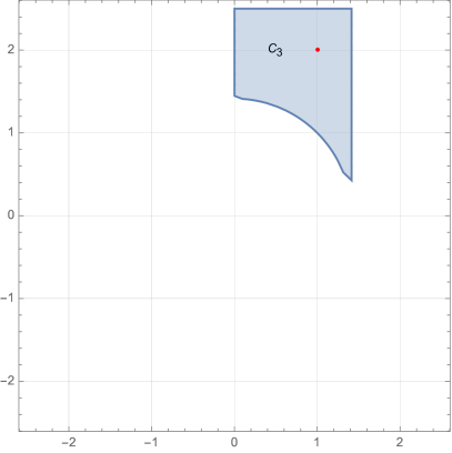
Figure 1: CAD of the polynomial $f=x^{2}+y^{2}-2$ from Example 4 (left). Computed cell capturing the model $(1,2)$ of Example 5 (right).

The theory and practice of CAD is heavily dependent on the ordering of variables involved. For this paper we always assume the CAD order to be the same as the order of the defined polynomials (e.g., $x_{1}<x_{2}<\ldots<x_{n}$). Every CAD cell is cylindrical in nature, and can be described by constraints where every dimension of the cell (called a level) can be completely defined by relying only on the previous dimensions. We illustrate this through an example.

Example 4

Consider the polynomial $f=x^{2}+y^{2}-2\in\mathbb{Z}[x,y]$. A CAD of $f$ is depicted in Figure 1 (left). The cell $C_{1}$ is defined by two constraints:

$$C^{y}_{1} \equiv y>_{r}\operatorname{\mathsf{root}}(x^{2}+y^{2}-2,2,y)\enspace,$$

$$C^{x}_{1} \equiv x>_{r}\operatorname{\mathsf{root}}(x^{2}-2,1,x)\wedge x<_{r}\operatorname{\mathsf{root}}(x^{2}-2,2,x)\enspace.$$

Constraint $C^{x}_{1}$ is at the first level (it’s a constraint on $x$ only), while constraint $C^{y}_{1}$ is at the second level and relates variables $x$ and $y$. The full cell description is then $C_{1}\equiv C_{1}^{x}\wedge C_{1}^{y}$. The green cell $C_{2}$ can be described by $C^{y}_{2}\equiv\top$ and $C^{x}_{2}\equiv x>_{r}\operatorname{\mathsf{root}}(x^{2}-2,2,x)$, with the full description $C_{2}\equiv C_{2}^{y}\wedge C_{2}^{x}$.

Model-based decision procedures such as NLSAT rely on CAD construction but do not construct the complete CAD decomposition. Instead, given a point in $\mathbb{R}^{n}$ they can construct a single cell of a CAD in a model-driven fashion. For more information about this approach, we refer the reader to [27, 4]. For our purposes we abstract the cell construction, and denote with $\mathsf{describeCell}(F,M)$ the function that, given a set of polynomials $F$, returns a description of a CAD cell of $F$ that contains the model $M$.

Following the terminology used in CAD, we say that a non-empty connected subset of $\mathbb{R}^{k}$ is a region. A set of polynomials $\{f_{1},\ldots f_{s}\}\subset\mathbb{Z}[\vec{y},x]$, with $\vec{y}=\langle y_{1},\ldots,y_{n}\rangle$, is said to be delineable in a region $S\subseteq\mathbb{R}^{n}$ if for every $f_{i}$ (and $f_{j}$) from the set, the following properties are invariant for any $\vec{\alpha}\in S$:

1. the total number of complex roots of $f_{i}(\vec{\alpha},x)$;

2. the number of distinct complex roots of $f_{i}(\vec{\alpha},x)$;

3. the number of common complex roots of $f_{i}(\vec{\alpha},x)$ and $f_{j}(\vec{\alpha},x)$.

Delineability has important consequences on the number and arrangement of real roots of polynomials $f_{i}$. As explained by the following theorem, if a set of polynomials $F$ is delineable on a region $S$, then the number of real roots of the polynomials does not change on $S$. Moreover, these roots maintain their relative order on the whole of $S$.

Theorem 4.1 (Corollary 8.6.5 of [40])

Let $F$ be a set of polynomials in $\mathbb{Z}[\vec{y},x]$, delineable in a region $S\subset\mathbb{R}^{n}$. Then, the real roots of $F$ vary continuously over $S$, while maintaining their order.

For a polynomial $f\in\mathbb{Z}[\vec{x}]$ and model $M=\{\vec{x}\mapsto\vec{v}\}$, we denote with $\operatorname{\mathsf{sgncstr}}(f,M)$ the polynomial constraint that matches the sign of $f$ in $M$, i.e.

$$\operatorname{\mathsf{sgncstr}}(f,M)=\begin{cases}f<0&\text{ if }\operatorname{\mathsf{sgn}}(f(\vec{v}))<0\\ f>0&\text{ if }\operatorname{\mathsf{sgn}}(f(\vec{v}))>0\\ f=0&\text{ if }\operatorname{\mathsf{sgn}}(f(\vec{v}))=0\\ \end{cases}$$

As described above, a CAD cell can be succinctly described by relying on extended polynomial constraints. We now show that the description of the cell can be reduced to basic polynomial constraints.

Lemma 3

Let $f_{i}\in\mathbb{Z}[y_{1},\ldots,y_{n},x]$ be two polynomials of degrees $m_{i}$, and $F_{i}\equiv x\;\triangledown_{r}\;\operatorname{\mathsf{root}}(f_{i},k_{i},x)$ be extended polynomial constraints of a cell description. Let $S$ be a region of $\mathbb{R}^{n}$ where $\{f_{1},f_{2}\}$ are delineable and let $M=\{\vec{y}\mapsto\vec{v},x\mapsto\alpha\}$ be a model such that $\vec{v}\in S$. Then, for all $\vec{y}\in S$ it holds that

$$\bigwedge_{i=0}^{m_{1}-1}\operatorname{\mathsf{sgncstr}}(f_{1}^{(i)},M)\wedge\bigwedge_{i=0}^{m_{2}-1}\operatorname{\mathsf{sgncstr}}(f_{2}^{(i)},M)\Rightarrow F_{1}\wedge F_{2}\enspace.$$

The proof of this lemma is relatively straightforward. The CAD cell description for level $x$ represents an entry in the sign table of $f_{1}$ and $f_{2}$ (with no roots in between). A part of this sign table entry that contains $M$ can be described with the signs of all the derivatives of $f_{1}$ and $f_{2}$ as long as we can guarantee that neither the arrangement nor the number of roots $f_{1}$ and $f_{2}$ change. But, this is guaranteed by $f_{1}$ and $f_{2}$ being delineable on $S$, so the lemma holds.

As a corollary to this lemma, in the context of CAD cell construction around a model $M$, we can replace any extended constraints describing a cell $C$ with basic constraints stating that the signs of the polynomial derivatives are the same as in $M$. This results in a valid CAD subcell $C^{\prime}\subseteq C$ for the same polynomials, that still contains the model $M$. We denote the function that constructs a basic CAD cell description of a set of polynomials $F$ capturing the model $M$ with $\mathsf{describeCellBasic}(F,M)$.

Example 5

Based on Example 4, we can construct a cell around the model $M=\{x\mapsto 1,y\mapsto 2\}$. Function $\mathsf{describeCellBasic}(F,M)$ will return the constraints

$$C^{y}_{3} \equiv(x^{2}+y^{2}>2)\wedge(y>0)\enspace,$$

$$C^{x}_{3} \equiv(x^{2}<2)\wedge(x>0)\enspace.$$

The full cell description is then $C_{3}\equiv C_{3}^{x}\wedge C_{3}^{y}$. Note that this cell is smaller than the cell $C_{1}$ from Example 4. This reduction in size is generally undesirable, but it is a price to pay for having the description in a simpler language.

Interpolation without extended constraints.

We now show how the cell construction described above can be used to remove extended polynomial constraints from a model interpolant. Assume a clausal model interpolant

$$I=(L_{1}\vee\ldots\vee L_{i}\vee\ldots\vee L_{N})$$

that is implied by formula $A$ and refutes a model $M=\{\vec{x}\mapsto\vec{v}\}$, i.e., all literals of $I$ evaluate to $\bot$ in $M$. Assume also that some literal $L_{i}$ contains an extended polynomial constraint $x_{n}\;\triangledown_{r}\;\operatorname{\mathsf{root}}(f,k,x_{n})$, with $f\in\mathbb{Z}[\vec{x}]$. We aim to replace the extended literal $L_{i}$ with literals over basic polynomial constraints. To do so, we need to find literals $L^{1}_{i},\ldots,L^{m}_{i}$ such that $L_{i}\Rightarrow(L^{1}_{i}\vee\ldots\vee L^{m}_{i})$ and all literals $L^{j}_{i}$ evaluate to $\operatorname{\bot}$ in $M$. Then, the clause

$$I^{\prime}=(L_{1}\vee\ldots\vee L^{1}_{i}\vee\ldots L^{m}_{i}\vee\ldots\vee L_{N})$$

will also be a model interpolant implied by $A$ that refutes the model $M$.

We can construct the literals $L^{j}_{i}$ using single cell construction as follows. We create a description of the CAD cell of the polynomial $f$ from $L_{i}$ that captures the model $M$. Let $\mathsf{describeCellBasic}(\{f\},M)=D_{1}\wedge\ldots\wedge D_{m}$ be this description. Since the cell fully captures the behavior of $f$ around $M$, we know that $D_{1}\wedge\ldots\wedge D_{m}\Rightarrow\neg L_{i}$ and all literals $D_{j}$ evaluate to $\operatorname{\top}$. Therefore, we can use the cell description to eliminate the extended literal $L_{i}$, obtaining the clause

$$I^{\prime}=(L_{1}\vee\ldots\vee\neg D_{i}\vee\ldots\neg D_{m}\vee\ldots\vee L_{n})$$

By continuing this process, we can replace all extended literals from a model interpolant, to obtain a model interpolant in the basic language of polynomial constraints.

Example 6

Consider the model interpolant $I=\neg(x>_{r}\operatorname{\mathsf{root}}(x^{2}-2,2,x)$ from Example 3 that refutes the model $M=\{x\mapsto 2\}$. To express $I$ in terms of basic polynomials constraints we first construct a regular CAD cell of $f=x^{2}-2$ around $M$. In this case this cell is simply $x>_{r}\operatorname{\mathsf{root}}(x^{2}-2,2,x)$. Then, we use Lemma 3 to construct a basic CAD cell description as $(x^{2}>2)\wedge(x>0)$. Finally, the simplified interpolant is $I^{\prime}=\neg(x^{2}>2)\vee\neg(x>0)$.

Termination.

With the description of the interpolation procedure complete, we discuss the termination of the procedure. To do so, we fix the formula $A(\vec{x},\vec{y})$ of Definition 3 and we assume a fixed order of variables that ensures $y_{i}<x_{i}$. Since the MCSAT decision procedure on which we rely is based on CAD, we can put a bound on the set of literals that can ever appear in a model interpolant from the formula $A$ to an arbitrary model $M$. Let $P_{A}$ be the set of polynomials appearing in $A$, and let $P=\mathsf{P}(P_{A})$ denote the closure of the set $P_{A}$ under the CAD projection operator used by the decision procedure. Finally, let $P^{\prime}$ be the closure of $P$ under derivatives. The set of polynomial constraints that can appear in the interpolant $I$ is limited to basic polynomial constraints over polynomials in $P^{\prime}$. This means that the procedure mcsat::check() can only generate a finite number of model interpolants and therefore has the finite convergence property.

Lemma 4

Assuming a fixed variable order, the mcsat::check() procedure has the finite convergence property for nonlinear arithmetic formulas.

Together with Lemma 2, this lemma implies that our interpolation procedure for the theory of nonlinear arithmetic terminates.

Model generalization.

We now proceed to show how the CAD cell construction can be used in a natural way to provide model-driven generalization. As in Definition 2, assume a formula $F(\vec{x},\vec{y})$ such that $F$ is true in a model $M$. Our aim is to construct a formula $G(\vec{x})$ that generalizes the model $M$ and still guarantees a solution to $F$.

Following the approach of [15], we do this in two steps. First, we construct an implicant $B$ of $F$ based on the model $M$. Then, we eliminate the variables $\vec{y}$ from $B$, again relying on the model $M$. The implicant $B$ is a conjunction of literals that implies $F$ and such that $B$ is true in M. The implicant can be computed by a top-down traversal of the formula $F$ while using the model $M$ to evaluate the formula nodes (see, e.g., [15] for a detailed description). To find a formula $G$ such that $G\Rightarrow\exists\vec{y}\;.\;B$, we use CAD cell construction as follows. Let $P\subseteq\mathbb{Z}[\vec{x},\vec{y}]$ be the set of all polynomials appearing in $B$, and let the cell description of $P$ around $M$ be

$$\mathsf{describeCellBasic}(P,M)=D_{\vec{x}}\wedge D_{\vec{y}}\enspace.$$

Here, $D_{\vec{x}}$ denotes the description of cell levels of variables $\vec{x}$, while $D_{\vec{y}}$ denotes the description of cell levels of variables $\vec{y}$. Because of the cylindrical nature of CAD cells, and the order on variables $y_{i}$ and $x_{i}$, we are guaranteed that every solution of $D_{\vec{x}}$ can be extended to a solution of $D_{\vec{y}}$. Therefore we set the final generalization $G(x)\equiv D_{\vec{x}}$

Example 7 (Generalization)

Consider the formula $F\equiv(x^{2}+y^{2}<2)$ and the model $M=\{x\mapsto 1,y\mapsto 2\}$ that satisfies $F$, and let us compute a generalization $G(x)$ of $M$. First, we compute a CAD cell of $f=x^{2}+y^{2}-2$ as shown in Example 5. Then we drop the description of cell level $y$, to obtain the model generalization $G(x)\equiv(x^{2}<2)\wedge(x>0)$.

5 Evaluation

To the best of our knowledge, there is no clear metric for evaluating how good an interpolant is, or for comparing different interpolants. In this section, we first show two examples to illustrate the procedure and its applications. Then, we evaluate the effectiveness of our interpolation procedure on practical problems that arise from model-checking applications. To this end, we integrate the procedure into a model checker and evaluate whether the procedure is efficient, and can produce abstractions that help the model checker synthesize invariants and discover counter-examples.

We have implemented the reasoning procedures (solving modulo partial models and interpolation procedure) by extending the existing mcsat implementation of the yices2 SMT solver [14]. We used the libpoly library [31] for computing the model generalization and simplification of algebraic cells. Since yices2 is integrated into the sally model checker [30], we rely on the pdkind method [30] as the model checking engine (the user of interpolation) in our evaluation.

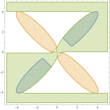
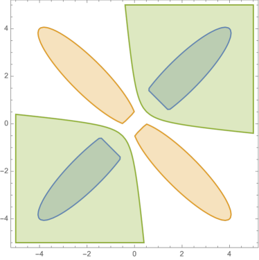
Figure 2: Illustration of interpolants from Example 8. In blue and orange are the feasible space of the formulas $A$ and $B$ (projected on $x$ and $y$). In green is the feasible space of the interpolant produced by our method (on the left) and the interpolant produced by [19] (on the right).

Example 8

We compare the style of interpolants generated by our new procedure with the ones generated by numerical approaches such as [19]. Example 4 from [19] considers two formulas of the form

$$A(x,y,a_{1},a_{2},b_{1},b_{2})\equiv(f_{1}\geq 0\wedge f_{2}\geq 0)\vee(f_{3}\geq 0\wedge f_{4}\geq 0)\enspace,$$

$$B(x,y,c_{1},c_{2},d_{1},d_{2})\equiv(g_{1}\geq 0\wedge g_{2}\geq 0)\vee(g_{3}\geq 0\wedge g_{4}\geq 0)\enspace.$$

The polynomials $f_{i}$ and $g_{i}$ involved in $A$ and $B$ are of degree 2. The right-hand side of Figure 2 shows the interpolant $I_{1}$ found by the approach in [19]. This interpolant is of the form $h(x,y)>0$, where $h$ is a polynomial degree two computed using semidefinite programming. Our approach, on the other hand, produces the interpolant $I_{2}$ shown on the left-hand side of Figure 2. This interpolant consists of 12 clauses, each containing 6–8 polynomial constraints over 16 different polynomials (8 linear, 8 of degree 2). The interpolant $I_{2}$ is ultimately produced from fragments of a CAD so its edges touch upon the critical points of the shape they were produce from (formula $A$). Interpolant $I_{1}$, on the other hand, has a simple form dictated by the method [19]. Which form is ultimately more useful depends on a particular application.

Example 9 (Cauchy-Schwartz)

As described in Example 1, we can model the computation of Cauchy-Schwarz inequality as a transition system $\operatorname{\mathfrak{S}}_{cs}$. Then we can prove the inequality correct if we can prove that the property $P_{cs}$ is valid in $\operatorname{\mathfrak{S}}_{cs}$. The pdkind model checking engine with the new interpolation procedure proves the property valid in 1s.

Benchmarks.

We run the evaluation on an existing set of nonlinear model-checking problems used by Cimatti, et al. [8]. This set consists of 114 benchmarks from various sources: handcrafted benchmarks, hybrid system verification, nuxmv benchmarks, C floating-point verification, and verification of Simulink models. The benchmark problems all contain transition systems with nonlinear behavior. For each problem, the goal is to prove or disprove a single invariant. We refer the reader to [8] for a more detailed description.

Evaluation.

Cimatti, et al. [8] present an abstraction approach based on incrementally more precise linear approximations of nonlinear polynomials. They show that this approach, implemented in the ic3-nra tool, is superior to other tools (such as, isat3 [36] and nuxmv [6] with upfront linear abstraction). Since our goal is to show the effectiveness of our interpolation procedure, rather than compare to many model checking engines, we keep the evaluation simple and only compare to ic3-nra. In addition, we include the k-induction engine kind of sally in the comparison to illustrate the importance of invariant inference and counter-example generation.

We ran the tools on the benchmark set with a 1h CPU timeout per problem. The results are shown in Table 3 and on the cactus plot in Figure 4. A scatter plot comparison of pdkind against ic3-nra and kind is shown in Figure 5.

Figure 3: Evaluation Results. For each tool, we report the number of solved problems, how many of the solved problems were valid and invalid, and the total time used to solve them. The rows correspond to different problem classes, and the bottom row reports the overall results for all 114 benchmarks.

. ic3-nra kind pdkind problem set solved valid/invalid time (s) solved valid/invalid time (s) solved valid/invalid time (s) handcrafted (14) 10 9/1 381 3 2/1 0 14 13/1 4 hycomp (7) 2 2/0 15 4 1/3 796 4 2/2 792 hyst (65) 39 32/7 404 25 13/12 50 38 26/12 42 isat3 (1) 0 0/0 0 0 0/0 0 0 0/0 0 isat3-cfg (10) 8 6/2 14 9 6/3 9 10 7/3 8 nuxmv (2) 2 2/0 158 0 0/0 0 1 1/0 1118 sas13 (13) 10 5/5 13 5 0/5 0 13 8/5 7 tcm (2) 2 2/0 1 2 2/0 0 2 2/0 0 73 58/15 986 48 24/24 855 82 59/23 1971

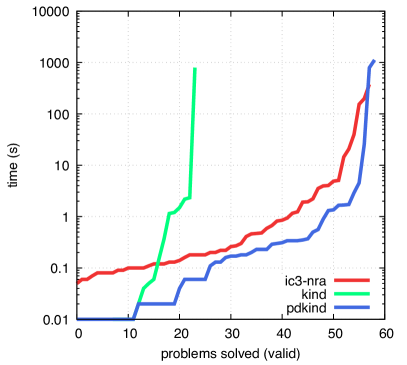
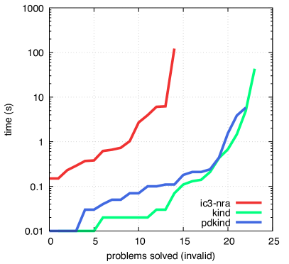
Figure 4: Cactus Plots Comparing the Performance of ic3-nra, kind, and pdkind. The $x$ axis is the number of problems solved (valid on the left, invalid on the right) and the $y$ axis is the time needed to solve the problem (log scale).

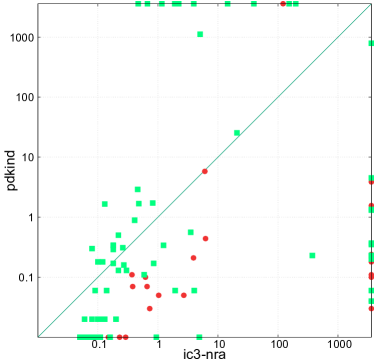
Figure 5: Scatter Plots Comparing the Performance of ic3-nra and kind with pdkind. Green squares represent problems that are valid. Red dots represent problems that are invalid. Each axis represents the time it took the tool to solve the problem (log scale).

As can be seen from Table 3, the results are positive. The pdkind engine with the new interpolation method can prove more properties and find more counter-examples than the state-of-the-art ic3-nra.

Out of 59 properties that pdkind shows correct, 36 cannot be proved by kind. This means that these properties are likely not $k$-inductive and that the interpolants produced by our procedure are valuable abstractions in invariant inference. Similarly, ic3-nra proves 37 properties that are not $k$-inductive. As can be seen from the scatter plot in Figure 5, there are properties that pdkind can prove than ic3-nra cannot, and vice versa (11 and 10, respectively). This is to be expected from a difficult domain, but it also means that the interpolation and the abstraction approach (or other methods) can be used to complement each other.

As for the invalid properties, since our interpolation method (and thus pdkind) is based on complete and precise reasoning, while ic3-nra relies on abstraction, it is to be expected that pdkind can prove more properties invalid. Furthermore, the comparison with kind in Figure 5 shows that pdkind finds all but one counter-examples that kind does in a similar amount of time. We see this as a confirmation that the interpolation and generalization methods are effective, i.e., they do not impede the search for counter-examples.

5.1 Related work

There is ample literature on interpolation for different fragments of nonlinear arithmetic. Existing methods can roughly be classified into two categories: approaches based on interval reasoning, and approaches based on semidefinite programming. Interval reasoning techniques (e.g., [35, 20, 36]) construct a proof of unsatisfiability through interval slicing and propagation. From such a proof, interpolants can be built using proof-based interpolation techniques. While incomplete, interval-based techniques can be very effective on problems that are hard for complete techniques. Moreover they can support more polynomial functions (e.g., elementary functions, ODEs). Our procedure is complete, but it is limited to the theories supported by MCSAT. The approaches based on semidefinite programming [12, 18, 19] generally approach the interpolation problem by restricting both the fragment of arithmetic (e.g., bounded constraints, same set of variables, quadratic constraints) and the shape of the interpolant (a single polynomial constraint) so that the interpolant itself can be represented as a semidefinite optimization problem. When they apply, these procedures are also very effective but they suffer from numerical imprecision, requiring special care to account for these errors and making them difficult to use in formal verification. In contrast, out procedure applies to nonlinear arithmetic as a whole. It relies on symbolic techniques, which are not subject to numerical errors. It is precise and complete, and it produces clausal interpolants.

The core ideas beyond our model-based interpolation approach were presented at the Boolean level as SAT solving with assumptions [17]. Closest to our work is the work of Schindler and Jovanović [42] where a similar model-based approach to interpolation is applied to conjunctions of linear arithmetic constraints based on conflict resolution. Our work is more general as it applies to formulas other than conjunctions, and it is applicable to a wider range of theories.

6 Conclusion and Future Work

We have presented a general approach for interpolation in SMT. This novel approach relies on a mode of interaction with the SMT solver that can check a formula for satisfiability modulo a partial model and, if the formula is unsatisfiable, can return a model interpolant that refutes the model. This allows us to develop a first complete interpolation procedure for nonlinear arithmetic. We have implemented the new procedure in the yices2 SMT solver and evaluated the interpolation procedure on model-checking problems. The new procedure seems to be effective in practice and opens new possibilities in the verification of systems that contain nonlinear behavior. Additionally, we show interesting examples of how the procedure can be used in automating induction proofs in mathematics.

The interpolation procedure that we presented can support other theories available in MCSAT (e.g., uninterpreted functions [28], bit-vectors [22], nonlinear integer arithmetic [27]). We plan to explore interpolation in these theories in more detail, and in the contexts where interpolation can be beneficial (e.g., model checking, quantified reasoning, termination, and proof generation).

References

- [1] C. Barrett and C. Tinelli. Satisfiability modulo theories. In Handbook of Model Checking, pages 305–343. Springer, 2018.
- [2] S. Basu, R. Pollack, and M.-F. Roy. Algorithms in real algebraic geometry. Springer, 2006.
- [3] S. Bayless, C. G. Val, T. Ball, H. H. Hoos, and A. J. Hu. Efficient modular SAT solving for IC3. In S. Ray and B. Jobstmann, editors, 2013 Formal Methods in Computer-Aided Design, pages 149–156. IEEE, 2013.
- [4] C. W. Brown and M. Košta. Constructing a single cell in cylindrical algebraic decomposition. Journal of Symbolic Computation, 70:14–48, 2015.
- [5] B. Buchberger, G. E. Collins, R. Loos, and R. Albrecht, editors. Computer algebra. Symbolic and algebraic computation. Springer, 1982.
- [6] R. Cavada, A. Cimatti, M. Dorigatti, A. Griggio, A. Mariotti, A. Micheli, S. Mover, M. Roveri, and S. Tonetta. The nuXmv symbolic model checker. In A. Biere and R. Bloem, editors, International Conference on Computer Aided Verification, pages 334–342. Springer, 2014.
- [7] B. F. Caviness and J. R. Johnson, editors. Quantifier Elimination and Cylindrical Algebraic Decomposition. Texts and Monographs in Symbolic Computation. Springer, 2004.
- [8] A. Cimatti, A. Griggio, A. Irfan, M. Roveri, and R. Sebastiani. Invariant checking of NRA transition systems via incremental reduction to LRA with EUF. In A. Legay and T. Margaria, editors, International Conference on Tools and Algorithms for the Construction and Analysis of Systems, pages 58–75. Springer, 2017.
- [9] A. Cimatti, A. Griggio, and R. Sebastiani. Efficient interpolant generation in satisfiability modulo theories. In C. R. Ramakrishnan and J. Rehof, editors, International Conference on Tools and Algorithms for the Construction and Analysis of Systems, pages 397–412. Springer, 2008.
- [10] G. E. Collins. Quantifier elimination for real closed fields by cylindrical algebraic decomposition. In H. Brakhage, editor, Automata Theory and Formal Languages, pages 134–183. Springer, 1975.
- [11] W. Craig. Three uses of the Herbrand-Gentzen theorem in relating model theory and proof theory. The Journal of Symbolic Logic, 22(3):269–285, 1957.
- [12] L. Dai, B. Xia, and N. Zhan. Generating non-linear interpolants by semidefinite programming. In N. Sharygina and H. Veith, editors, International Conference on Computer Aided Verification, pages 364–380. Springer, 2013.
- [13] L. De Moura and D. Jovanović. A model-constructing satisfiability calculus. In R. Giacobazzi, J. Berdine, and I. Mastroeni, editors, International Workshop on Verification, Model Checking, and Abstract Interpretation, pages 1–12. Springer, 2013.
- [14] B. Dutertre. Yices 2.2. In A. Biere and R. Bloem, editors, International Conference on Computer Aided Verification, pages 737–744. Springer, 2014.
- [15] B. Dutertre. Solving exists/forall problems with Yices. In 13th International Workshop on Satisfiability Modulo Theories, 2015.
- [16] N. Eén and N. Sörensson. An extensible SAT-solver. In E. Giunchiglia and A. Tacchella, editors, International conference on theory and applications of satisfiability testing, pages 502–518. Springer, 2003.
- [17] N. Eén and N. Sörensson. Temporal induction by incremental SAT solving. Electronic Notes in Theoretical Computer Science, 89(4):543–560, 2003.
- [18] T. Gan, L. Dai, B. Xia, N. Zhan, D. Kapur, and M. Chen. Interpolant synthesis for quadratic polynomial inequalities and combination with EUF. In N. Olivetti and A. Tiwari, editors, International Joint Conference on Automated Reasoning, pages 195–212. Springer, 2016.
- [19] T. Gan, B. Xia, B. Xue, N. Zhan, and L. Dai. Nonlinear Craig interpolant generation. In S. K. Lahiri and C. Wang, editors, International Conference on Computer Aided Verification, pages 415–438. Springer, 2020.
- [20] S. Gao and D. Zufferey. Interpolants in nonlinear theories over the reals. In M. Chechik and J.-F. Raskin, editors, International Conference on Tools and Algorithms for the Construction and Analysis of Systems, pages 625–641. Springer, 2016.
- [21] S. Gerhold and M. Kauers. A procedure for proving special function inequalities involving a discrete parameter. In X.-S. Gao and G. Labahn, editors, Proceedings of the 2005 international symposium on Symbolic and algebraic computation, pages 156–162, 2005.
- [22] S. Graham-Lengrand, D. Jovanović, and B. Dutertre. Solving bitvectors with MCSAT: explanations from bits and pieces. In N. Peltier and V. Sofronie-Stokkermans, editors, International Joint Conference on Automated Reasoning, pages 103–121. Springer, 2020.
- [23] T. A. Henzinger, R. Jhala, R. Majumdar, and K. L. McMillan. Abstractions from proofs. ACM SIGPLAN Notices, 39(1):232–244, 2004.
- [24] K. Hoder and N. Bjørner. Generalized property directed reachability. In A. Cimatti and R. Sebastiani, editors, International Conference on Theory and Applications of Satisfiability Testing, pages 157–171. Springer, 2012.
- [25] J. Hoenicke and T. Schindler. Efficient interpolation for the theory of arrays. In D. Galmiche, S. Schulz, and R. Sebastiani, editors, International Joint Conference on Automated Reasoning, pages 549–565. Springer, 2018.
- [26] G. Huang. Constructing Craig interpolation formulas. In D.-Z. Du and M. Li, editors, Computing and Combinatorics, pages 181–190. Springer, 1995.
- [27] D. Jovanović. Solving nonlinear integer arithmetic with MCSAT. In A. Bouajjani and D. Monniaux, editors, International Conference on Verification, Model Checking, and Abstract Interpretation, pages 330–346. Springer, 2017.
- [28] D. Jovanovic, C. Barrett, and L. De Moura. The design and implementation of the model constructing satisfiability calculus. In S. Ray and B. Jobstmann, editors, 2013 Formal Methods in Computer-Aided Design, pages 173–180. IEEE, 2013.
- [29] D. Jovanović and L. De Moura. Solving non-linear arithmetic. In B. Gramlich, D. Miller, and U. Sattler, editors, International Joint Conference on Automated Reasoning, pages 339–354. Springer, 2012.
- [30] D. Jovanović and B. Dutertre. Property-directed k-induction. In R. Piskac, M. Talupur, and H. Veith, editors, 2016 Formal Methods in Computer-Aided Design (FMCAD), pages 85–92. IEEE, 2016.
- [31] D. Jovanović and B. Dutertre. LibPoly: A library for reasoning about polynomials. In Proc. 15th International Workshop on Satisfiability Modulo Theories (SMT 2017), 2017.
- [32] D. Kapur, R. Majumdar, and C. G. Zarba. Interpolation for data structures. In M. Young and P. Devanbu, editors, Proceedings of the 14th ACM SIGSOFT international symposium on Foundations of Software Engineering, pages 105–116, 2006.
- [33] A. Komuravelli, A. Gurfinkel, and S. Chaki. SMT-based model checking for recursive programs. Formal Methods in System Design, 48(3):175–205, 2016.
- [34] J. Krajíček. Interpolation theorems, lower bounds for proof systems, and independence results for bounded arithmetic. The Journal of Symbolic Logic, 62(2):457–486, 1997.
- [35] S. Kupferschmid and B. Becker. Craig interpolation in the presence of non-linear constraints. In U. Fahrenberg and S. Tripakis, editors, International Conference on Formal Modeling and Analysis of Timed Systems, pages 240–255. Springer, 2011.
- [36] A. Mahdi, K. Scheibler, F. Neubauer, M. Fränzle, and B. Becker. Advancing software model checking beyond linear arithmetic theories. In R. Bloem and E. Arbel, editors, Haifa Verification Conference, pages 186–201. Springer, 2016.
- [37] K. L. McMillan. An interpolating theorem prover. Theoretical Computer Science, 345(1):101–121, 2005.
- [38] K. L. McMillan. Quantified invariant generation using an interpolating saturation prover. In C. R. Ramakrishnan and J. Rehof, editors, International Conference on Tools and Algorithms for the Construction and Analysis of Systems, pages 413–427. Springer, 2008.
- [39] K. L. McMillan. Interpolation: Proofs in the service of model checking. In Hanbook of Model-Checking. Springer, 2014.
- [40] B. Mishra. Algorithmic algebra. Springer, 1993.
- [41] P. Pudlák. Lower bounds for resolution and cutting plane proofs and monotone computations. The Journal of Symbolic Logic, 62(3):981–998, 1997.
- [42] T. Schindler and D. Jovanović. Selfless interpolation for infinite-state model checking. In I. Dilig and J. Palsberg, editors, International Conference on Verification, Model Checking, and Abstract Interpretation, pages 495–515. Springer, 2018.