WISDOM Project – IX. Giant Molecular Clouds in the Lenticular Galaxy NGC4429: Effects of Shear and Tidal Forces on Clouds
Abstract
We present high spatial resolution ( pc) Atacama Large Millimeter/sub-millimeter Array 12CO observations of the nearby lenticular galaxy NGC4429. We identify giant molecular clouds within the pc radius molecular gas disc. The clouds generally have smaller sizes and masses but higher surface densities and observed linewidths than those of Milky Way disc clouds. An unusually steep size – line width relation () and large cloud internal velocity gradients ( – km s-1 pc-1) and observed Virial parameters () are found, that appear due to internal rotation driven by the background galactic gravitational potential. Removing this rotation, an internal Virial equilibrium appears to be established between the self-gravitational () and turbulent kinetic () energies of each cloud, i.e. . However, to properly account for both self and external gravity (shear and tidal forces), we formulate a modified Virial theorem and define an effective Virial parameter (and associated effective velocity dispersion). The NGC4429 clouds then appear to be in a critical state in which the self-gravitational energy and the contribution of external gravity to the cloud’s energy budget () are approximately equal, i.e. . As such, and most clouds are not virialised but remain marginally gravitationally bound. We show this is consistent with the clouds having sizes similar to their tidal radii and being generally radially elongated. External gravity is thus as important as self-gravity to regulate the clouds of NGC4429.
keywords:
galaxies: elliptical and lenticular, cD – galaxies: individual: NGC4429 – galaxies: nuclei – galaxies: ISM – ISM: clouds – radio lines: ISM1 Introduction
It is well-known that giant molecular clouds (GMCs) are the major gas reservoirs for star formation (SF) and the sites where essentially all stars are born. Understanding the properties of GMCs is thus key to unraveling the interplay between gas and stars within galaxies. Early GMC studies were restricted to our own Milky Way (MW) and the late-type galaxies (LTGs) in our Galactic neighbourhood (e.g. Engargiola et al., 2003; Rosolowsky, 2005, 2007; Rosolowsky et al., 2007; Gratier et al., 2012; Colombo et al., 2014; Wu et al., 2017; Faesi et al., 2018), where GMCs have relatively uniform properties and generally follow the so-called Larson relations (between size, velocity dispersion and luminosity; e.g. Blitz et al. 2007; Bolatto et al. 2008). However, more recent studies of other local galaxies have raised doubts on the universality of cloud properties. The cloud properties in some LTGs (such as M51 and NGC253) vary with galactic environment and do not universally obey the usual scaling relations (e.g. Hughes et al., 2013; Leroy et al., 2015; Schruba et al., 2019). The first study of individual GMCs in an early-type galaxy (ETG; NGC4526) has also clearly shown that the clouds in that galaxy do not follow the usual size – linewidth correlation and tend to be more luminous, denser and to have larger velocity dispersions than the GMCs in the MW and other Local Group galaxies (Utomo et al., 2015). The differences in NGC4526 may be due to a higher interstellar radiation field (and/or cloud extinctions), a different external pressure relative to each cloud’s self-gravity, and/or different galactic dynamics. GMCs in ETGs seem to have shorter orbital periods and be subjected to stronger shear/tidal forces, analogous to the highly dynamic environment in the MW central molecular zone (CMZ; e.g. Kruijssen et al. 2019; Henshaw et al. 2019; Dale et al. 2019). Although we are entering an era of large surveys of GMC populations (e.g. Sun et al., 2018), current samples of ETGs are still very limited. More studies of GMCs in varied LTGs and ETGs are thus required to provide a comprehensive census of GMC properties across different galaxy environments.
A model introduced by Meidt et al. (2018) suggests that gas motions at the cloud scale combine the effects of gas self-gravity and the gas response to the forces exerted by the background host galaxy. In the ETG NGC4526, the gas motions at cloud scales appear to be driven by the galactic potential. The measured line widths of the GMCs are much larger than their Virial line widths (the line widths predicted by assuming the clouds’ Virial masses are equal to their gaseous masses), an effect that appears to be due to dominant gas motions associated with the background galactic potential. Cloud-scale velocity gradients aligned with the large-scale velocity field indeed suggest a dominance of rotational motions due to the galactic potential (Utomo et al., 2015). It is thus important to investigate whether cloud-scale gas motions are generally dominated by motions due to self-gravity (generally random) or motions due to the galactic potential (generally circular), as this has implications for the observed size – linewidth relation, the Virial parameter, cloud morphologies and the processes governing star formation (Meidt et al., 2018).
The dynamical state of a molecular cloud provides important insights into its evolution. It also plays an important role to determine its ability to form stars and stellar clusters (e.g. Hennebelle & Chabrier, 2013; Padoan et al., 2017). In most Virial balance analyses of molecular clouds, the gravitational term entering the Virial theorem includes only the cloud’s own self-gravitational energy. However, in some galactic environments (e.g. in galactic nuclei), the external (i.e. galactic) gravitational potential could also play an important role to regulate the cloud dynamics (e.g. Rosolowsky & Blitz, 2005; Thilliez et al., 2014; Yusef-Zadeh et al., 2016). To analyse the Virial balance of GMCs in such environments, one thus needs to add another gravitational term related to the background gravitational field (e.g. Ballesteros-Paredes et al., 2009; Chen et al., 2016).
The net effect of the external gravitational potential on the dynamics of GMCs should however also include an additional kinetic energy term related to the gas motions driven by the galactic potential, as they provide another source of support against the cloud’s self-gravity. In this paper, we therefore revisit the Virial theorem by adding two crucial terms that take into account the background galactic gravitational potential: an external gravitational energy term and a kinetic energy term associated with the gas motions due to galactic potential. Although an extended Virial theorem including a background tidal field has been formulated before (see, e.g., Chen et al., 2016), our resulting Virial equation contains new terms that were previously missing and is thus more general.
Early studies of GMCs suggested they are long-lived, quasi-equilibrium entities, isolated from their interstellar environment (e.g. Solomon et al., 1987; Elmegreen, 1989; Blitz, 1993). However, recent findings that the properties of GMCs vary with galactic environment imply that the clouds are not decoupled from their surroundings (e.g. Hughes et al., 2013; Colombo et al., 2014; Faesi et al., 2018). The main physical factors determining cloud properties include: (1) the interstellar radiation field (e.g. McKee, 1989); (2) large-scale dynamics (e.g. galactic tides and shear due to differential galactic rotation; Dib et al. 2012; Meidt et al. 2015; Melchior & Combes 2017); (3) interstellar gas pressure (e.g. Heyer et al., 2009; Hughes et al., 2013; Meidt, 2016); and (4) the large-scale atomic gas distribution and H i column density (e.g. Engargiola et al., 2003; Blitz et al., 2007; Rosolowsky et al., 2007). In this work, we will focus on the roles of galactic tide/shear to regulate the properties of GMCs. One of our main purposes is indeed to quantitatively investigate the effects of galactic tidal and shear forces on the physical properties and dynamical states of the clouds.
We note an important conceptual point. We will not assume here that the clouds are in dynamical equilibrium, to then infer the clouds’ gravitational motions due to the external (i.e. galactic) potential. Instead, we will attempt to directly estimate the clouds’ gravitational motions due to the external potential, to then infer whether the clouds are indeed in dynamical equilibrium or not. The question of whether GMCs are in dynamical equilibrium (and thus long-lived) or out of equilibrium (and thus transient) has remained unanswered for decades. We thus believe this approach is not only well-justified and worthwhile, but ultimately desirable.
The mm-Wave Interferometric Survey of Dark Object Masses (WISDOM) aims to use the high angular resolution of the Atacama Large Millimeter/sub-millimeter Array (ALMA) to study: (1) the masses and properties of the supermassive black holes (SMBHs) lurking at the centres of galaxies (e.g. Onishi et al., 2017; Davis et al., 2017; Davis et al., 2018; Smith et al., 2019; North et al., 2019; Smith et al., 2020a, b); (2) the physical properties and dynamics of GMCs in the central parts of the same galaxies. As part of WISDOM, we analyse here the properties and dynamics of individual GMCs in the bulge of NGC4429, an SA0-type galaxy located in the centre of the Virgo cluster. This paper is the first of a series studying the GMCs in WISDOM galaxies, and it introduces many of the methods and tools we will use to identify GMCs and analyse their properties and dynamics. The paper is structured as follows. In Section 2 we describe the data and the methodology used to identify GMCs in NGC4429. We use a modified version of the code CPROPSTOO, that is more robust and efficient at identifying clouds in complex and crowded environments. The cloud properties, their probability distribution functions and their mass distribution functions are reported in Section 3. Our analysis of the kinematics of individual GMCs is presented in Section 4. We investigate the dynamical states of the GMCs utilising our modified Virial theorem (taking into account the background galactic gravitational potential) in Section 5. The shear motions within clouds, the effects of self-gravity and the cloud morphologies are discussed in Section 6. We conclude briefly in Section 7.
2 Data and Cloud Identification
2.1 Target
NGC4429 is a lenticular galaxy located in the centre of the Virgo cluster, with a bar and stellar inner ring morphology (Alatalo et al., 2013). It contains a nuclear dust disc visible in extinction against the stellar continuum in Hubble Space Telescope (HST) imaging (Fig. 1 and Davis et al. 2018). NGC4429 has a total stellar mass of , a luminosity-weighted stellar velocity dispersion within one effective radius km s-1 (Cappellari et al., 2013), and is a fast rotator (specific angular momentum within one effective radius ; Emsellem et al. 2011).
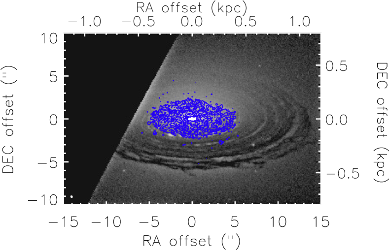
The total molecular gas mass of NGC4429 detected via 12CO(1-0) single-dish observations is (Young et al., 2011). The 12CO(1-0) Combined Array for Research in Millimeter-wave Astronomy (CARMA) interferometric map shows the molecular gas is co-spatial with the nuclear dust disc and regularly rotates in the galaxy mid-plane (Davis et al., 2011, 2013, 2018), with an inclination angle of (Davis et al., 2011; Alatalo et al., 2013). The 12CO(3-2) distribution is more compact than that of 12CO(1-0), the 12CO(3-2) gas being present only in the inner parts of the nuclear dust disc visible in HST images (see Fig. 1). The star formation rate (SFR) within this molecular gas disc has been estimated at yr-1 using mid-infrared and far-ultraviolet emission (Davis, 2014). The spatially-unresolved (sub-arcsecond) radio continuum emission from the central regions of NGC4429 implies the presence of a low-luminosity active galactic nucleus (LL-AGN; Nyland et al. 2016). The kinematics of the central CO gas, as probed by the same dataset as used here, imply the presence of a SMBH (Davis et al., 2018). Throughout this paper we assume a distance of Mpc for NGC4429 (Cappellari et al., 2011). One arcsecond then corresponds to a physical scale of pc.
2.2 Data
NGC4429 was observed in the 12CO(3-2) line (345 GHz) using ALMA as part of the WISDOM project. The data were calibrated and reduced in a standard manner (Davis et al., 2018), and the final 12CO(3-2) data cube we adopt has a synthesised beam of ( pc2) at a position angle of and a channel width of . It covers a region of ( pc2), thus comprising the entire nuclear dust and molecular gas disc. Pixels of were chosen as a compromise between spatial sampling and cube size, resulting in approximately pixels2 across the synthesised beam (Davis et al., 2018). Our spatial and spectral resolutions allow for reliable estimates of the radii and velocity dispersions of individual GMCs, that have a typical size of pc (Blitz, 1993) and a typical linewidth of several (e.g. Solomon et al., 1987). The root mean square (RMS) noise in line-free channels of the cube is mJy beam-1 ( K) in channels. The integrated 12CO(3-2) spectrum of NGC4429 exhibits the classic double-horn shape of a rotating disc, with a total flux of Jy km s-1.
As shown in Davis et al. (2018), the molecular gas disc of NGC4429 is flocculent. Our ALMA observations reveal that the CO(3-2) gas surface density does not decrease smoothly to our detection limit, but instead appears to be truncated at an inner radius of pc and an outer radius of pc (Davis et al., 2018). As mentioned above, the 12CO(3-2) disc thus lies only in the inner parts of the nuclear dust disc visible in HST images (see Fig. 1), and it has an extent smaller than that of the 12CO(1-0) emission (that extends to the edge of the nuclear dust disc; Davis et al. 2013). As CO(3-2) is excited in denser and warmer gas than CO(1-0) (with critical densities of and cm-3 and excitation temperatures of and K, respectively), we are likely to identify a cloud population that is associated with H ii regions and thus ongoing star formation at the centre of NGC4429 only. High-resolution observations of lower- CO transitions may be required to conduct a study of the NGC4429 GMC population over the entire molecular gas disc (if indeed additional clouds exist beyond the CO(3-2) extent probed here).
Continuum GHz emission was also detected in NGC4429, with a centre of and derived by Gaussian fitting. This position is consistent with the optical centre of NGC4429 (Adelman-McCarthy et al., 2008) and will be used as the centre of the galaxy in this work.
2.3 Cloud identification
We use our own modified version of the CPROPSTOO algorithms (Leroy et al., 2015) to identify cloud structures. CPROPSTOO is an updated version of CPROPS (Rosolowsky & Leroy, 2006), one of the cloud identification algorithms most widely used in the literature. The key modifications of CPROPSTOO compared to CPROPS were noted by Leroy et al. (2015): CPROPSTOO (1) deconvolves the beam in two dimensions; (2) employs a larger suite of size and linewidth measures, including measuring the area of and fitting an ellipse at the half maximum flux level (in addition to measuring the second moment); and (3) introduces additional extrapolation (aperture correction) approaches, that essentially assume a Gaussian distribution to extrapolate the ellipse fits. In this work we have further modified CPROPSTOO, to make it more robust when decomposing clouds in complex and crowded environments.
The cloud identification algorithm first calculates a spatially-varying estimate of the noise in the data cube, and then uses the noise cube generated to create a three-dimensional (3D) mask of bright emission. The mask initially includes only pixels where two adjacent channels (at the same position) both have intensities above . It is then expanded to include all neighbouring emission above a lower threshold – two adjacent channels above . The regions thus identified are referred to as “islands”. If an island has a projected area of less than two synthesised beams, it is assumed to be a noise peak and is removed from the mask. The resulting mask contains of the integrated flux of the galaxy, consistent with the fractions yielded by CPROPS in other studies of extragalactic clouds ( – ; Wong et al. 2011; Hughes et al. 2013; Donovan Meyer et al. 2013; Colombo et al. 2014; Leroy et al. 2015; Pan & Kuno 2017; Miura et al. 2018; Faesi et al. 2018; Wong et al. 2019; Imara & Faesi 2019). We checked the stringency of the mask by applying the same criteria to the inverted data set (scaled by ) and found no false positive, so the masking criteria are likely robust.
Once regions of significant emission (i.e. islands) have been identified, these islands are further decomposed into individual “cloud” structures. Clouds are identified as local maxima within a moving 3D box of area spaxels2 ( pc2) and velocity width of channels ( ). In our modified version of CPROPSTOO, we add another criterion to find local maxima, checking whether the ( pixels3) box centred on a local maximum also represents a local maximum on a larger scale, as suggested by Yang & Ahuja (2014). This is to eliminate the impact of noisy pixels or outliers, as a noise peak can easily become a local maximum within a single box, but much less so on a larger scale. We thus consider a ( pixels3) box centred on each local maximum, and require the sum of the flux densities in that box to be larger than that in all eight spatially-adjacent ( pixels3) boxes. The detection of local maxima in this way is much more robust and efficient.
For each local maximum, the original CPROPSTOO algorithm requires all emission uniquely associated with that maximum (i.e. all emission within the faintest intensity isosurface uniquely associated with that maximum) to have a minimum area (), minimum number of pixels () and minimum number of velocity channels (). It also requires the local maximum’s brightness temperature to lie at least above the merger level with any other maximum (i.e. the brightest contour level enclosing another local maximum). However, this decomposition algorithm often leads to cloud size and velocity dispersion distributions that peak around the chosen , and . This is a well-known bias that reflects the hierarchical structure of the ISM from parsec to kiloparsec scales (e.g. Verschuur, 1993; Hughes et al., 2013; Leroy et al., 2016). It becomes especially problematic for complex and crowded environments where the emission has low contrast and extends over a range of scales (e.g. the centre of M51; Hughes et al. 2013; Colombo et al. 2014). Small and tend to identify the sub-structures of a cloud (“over-decompositon”), whereas large and tend to miss out small structures (“under-decomposition”).
To remove this bias and identify cloud structures across multiple scales, we modified CPROPSTOO by setting each of and to a range of values rather than a single value. In our work, we assign a range of to spaxels (the synthesised beam area) with a step of spaxels (half the beam area), similarly in pixels for . We start by searching for the largest cloud structures using the largest ( spaxels) and ( pixels), and then repeat the search process to identify increasingly small clouds in the volume of the cube not yet assigned to any cloud. We use a (resp. ) spaxels (resp. pixels) smaller than the previous one at each step, until all the cloud structures larger than the beam size ( spaxels) are identified. As long as and cover large ranges, the final results hardly depend on the specified ranges. We are therefore able to remove two free parameters in the algorithm, making our results less arbitrary and more robust. A schematic of our modified CPROPSTOO technique is shown in Figure 2 for a one-dimensional (1D) line profile.
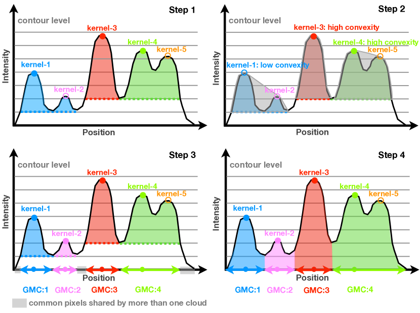
The main concern about our newly-developed approach, however, is that we may identify large clouds while ignoring potentially significant sub-structures. To solve this problem, we introduce a new parameter, , inspired by an analogous quantity in studies of biological structures (Lin et al., 2007), that describes how significant the sub-structure of a cloud is. The parameter is defined as the ratio of the volume of the cloud (i.e. the volume of its 3D intensity distribution) to the volume of the smallest convex hull encompassing all of its flux (i.e. the volume of the smallest convex envelope enclosing all of the cloud’s 3D intensity distribution; see the top-right panel of Fig. 2 for an example with a 1D line profile, i.e. a two-dimensional (2D) intensity distribution). The of a cloud should thus be close to if the cloud has only one intensity peak and no sub-structure, and be less than if the cloud has some sub-structures. The lower the value of , the more significant the sub-structure of a cloud. Our modified CPROPSTOO code requires all clouds to have a minimum (). Typical useful values are – , as determined by visual inspection, to ensure clouds are not over- or under-decomposed. In this work, we set to . Overall, our new refinements allows CPROPSTOO to identify structures over multiple scales, with less arbitrariness than previously.
We set the parameters and based on physical priors described by Rosolowsky & Leroy (2006), that suggest a cloud has a minimum velocity dispersion ( ) and K, motivated by the properties of Galactic GMCs. A factor of is applied to to convert the velocity dispersion to a full width at half maximum (FWHM). We set the parameters in physical units ( and K) rather than data units (channel, ) to reduce possible biases when comparing cloud properties from different observations. Our excellent spectral resolution (channel width of ) and sensitivity ( K) allow us to reach and thus use those physical parameters.
According to our algorithm, each surviving local maximum corresponds to a cloud. CPROPSTOO assigns the emission that is uniquely associated with each local maximum (i.e. the emission within the faintest intensity isosurface uniquely associated with that maximum) to that cloud. The remaining emission shared among clouds is then assigned to the “nearest” local maximum (i.e. the local maximum with the shortest path through the data cube from a given pixel). In our work, however, we apply a “friends-of-friends” algorithm to assign all remaining emission, as for the ClumpFind algorithm (Williams et al., 1994) and the original CPROPS code (Rosolowsky & Leroy, 2006). This friends-of-friends paradigm connects pixels according to the brightnesses of neighbouring pixels, without assuming a particular shape for the objects to decompose (Rosolowsky & Leroy, 2006). This method conserves flux, so that all the flux within the island regions is assigned to a particular cloud (Tasker & Tan, 2009). As each pair of pixels in a cloud can then be connected by a continuous path through that cloud, we avoid assigning disconnected pixels to the same cloud.
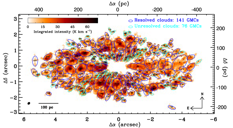
The resulting sample of GMCs in NGC4429 contains GMCs, of which are spatially resolved, shown in Fig. 3. The majority of the resolved clouds have a single-peaked Gaussian-like spatially-integrated line profile, although a few do reveal a double-peaked line profile possibly indicating significant rotation. Most line profiles are symmetric but a few are asymmetric, with significant skewness (blue or red wing). The clouds identified with our new refinements are fewer ( versus clouds), larger (median cloud size versus pc), more massive (median gaseous mass versus M⊙) and have velocity dispersions larger (median velocity dispersion versus km s-1) than those derived using the original CPROPSTOO code. They also span a larger range of sizes. A Gaussian fit to the size distribution yields a mean of pc and a standard deviation of pc for our spatially-resolved clouds (see Section 3.3), but pc and pc, respectively, for those identified using the original CPROPSTOO. The resolved clouds identified here also seem to have more regular morphologies, with a mean ( by construction) compared to (and of resolved clouds with ) for CPROPSTOO-identified clouds. This confirms that our approach and modified CPROPSTOO code have great potential to identify clouds over large spatial scales in crowded and complex environments (e.g. galactic centres and spiral arms).
3 Cloud Properties
3.1 Definition of GMC properties
Once all the pixels of every cloud have been identified, we calculate the physical properties of the clouds by following the standard CPROPSTOO/CPROPS definitions (Rosolowsky & Leroy, 2006). The CPROPSTOO algorithm applies moment methods to derive the size, linewidth and flux of a cloud from its distribution within a position-position-velocity data cube. One advantage of CPROPSTOO over other GMC identification algorithms is that it attempts to correct the measured cloud properties for the finite sensitivity and instrumental resolution (Rosolowsky & Leroy, 2006). To reduce the sensitivity bias, the algorithm measures the size, velocity width and luminosity as a function of the boundary intensity isosurface () and extrapolates them to the case of infinite signal-to-noise ratio (; i.e. K). The size and linewidth are extrapolated linearly, while the luminosity is extrapolated quadratically. To correct for the resolution bias, CPROPSTOO “deconvolves” the synthesised beam size from the measured extrapolated cloud size in two dimensions. Rosolowsky & Leroy (2006) argued that moment measurements combined with beam deconvolution and extrapolation represent a robust way to compare heterogeneous observations of molecular clouds.
Cloud centre. The central position (, ) and velocity () of each cloud are obtained directly from the intensity-weighted first spatial and velocity moment,
| (1) |
where () is the position of a given pixel, its velocity and its flux (brightness temperature), and the sums are over all pixels of each cloud.
Cloud size. The radius of each cloud is calculated as the geometric mean of the second spatial moment of the intensity distribution along the major and the minor axis:
| (2) |
where and are the deconvolved RMS spatial extent along the major and the minor axis, respectively, extrapolated to the K isosurface, and is a factor relating the one-dimensional RMS extent to the radius of a cloud. While formally depends on the shape and density profile of the cloud, we follow Solomon et al. (1987) and common practice and adopt whenever we need to evaluate expressions containing . The major and minor axes are thus defined as the principal axes of the moment of inertia tensor of the cloud (see Eq. 1 in Rosolowsky & Leroy 2006).
Cloud velocity dispersion. The observed (i.e. 1D) linewidth or velocity dispersion of each cloud is measured from the second moment of the intensity distribution along the velocity axis, extrapolated to K. To account for the potential bias toward a higher velocity dispersion due to the finite spectral resolution, we perform a deconvolution as suggested by Rosolowsky & Leroy (2006):
| (3) |
where is the extrapolated second moment along the velocity axis, is the channel width and is the standard deviation of a Gaussian that has an integrated area equal to a spectral channel of width .
The observed velocity dispersion includes the effects of turbulent motions, intrinsic rotation of the cloud, and shear motions due to the large-scale kinematics of the galactic disc (such as galactic rotation and streaming motions).
In our work, we introduce another measured velocity dispersion, , as defined by Utomo et al. (2015), although we adopt the notation of Henshaw et al. (2019). We first calculate the intensity-weighted mean velocity at each line of sight through a cloud (), and measure its offset with respect to the mean velocity at the cloud centre (). We assume that this offset () is produced by both intrinsic motions within the cloud and/or large-scale galactic disc motions, and thereby shift the velocities at each line of sight to match their mean velocity to that of the cloud centre (). We then measure the second moment of the shifted emission distribution along the velocity axis and extrapolate it to K. The final derived gradient-subtracted velocity dispersion, , is also deconvolved for the channel width as above. We thus obtain a measure of the turbulent (random) motions within the cloud only, free of any bulk motion.
Cloud luminosity. The CO(3-2) luminosity of each cloud is given by
| (4) |
where is the zeroth moment (total flux) of the cloud extrapolated to K using a quadratic extrapolation and is the distance to NGC4429.
Cloud gaseous mass. The CO luminosity-based mass of each cloud is obtained from using
| (5) |
where is the cloud’s CO(1-0) luminosity (see Eq. 4 above) and is the assumed CO-to-H2 conversion factor. The CO(3-2)/CO(1-0) intensity ratio was measured to be (in beam temperature units) overall in NGC4429 (Davis et al., 2018), and we assume that value for all the clouds here. We further adopt a standard Galactic conversion factor cm-2 (K km s-1)-1 (including the mass contribution from helium; Strong et al. 1988; Bolatto et al. 2013), commonly used in previous extragalactic studies (e.g. Hughes et al., 2013; Colombo et al., 2014; Utomo et al., 2015; Sun et al., 2018), although it has been suggested that this conversion factor depends on the environment of each molecular cloud, e.g. metallicity and radiation field (see Bolatto et al. 2013 for a review). The final gaseous mass of each cloud is thus obtained from
| (6) |
Cloud Virial mass. The Virial (i.e. dynamical) mass of each cloud is calculated with the formula
| (7) |
(MacLaren et al., 1988), where is the gravitational constant, the observed (i.e. 1D) cloud velocity dispersion, the cloud radius (see Eq. 2) and is a geometrical factor that quantifies the effects of inhomogeneities and/or non-sphericity of the cloud mass distribution on its self-gravitational energy. For a cloud in which the isodensity contours are homoeoidal ellipsoids, , where quantifies the effects of the inhomogeneities and those of the ellipticity (see Appendix A for more details on and ). We adopt for a spherical homogeneous (i.e. constant density) cloud whenever we need to evaluate . The Virial mass obtained from Eq. 7 assumes that each cloud is spherical and virialised (with isotropic velocity dispersions), with no magnetic support or pressure confinement. We note that, to investigate the dynamical state of each cloud in the presence of strong tidal/shear forces, in the sections that follow we will define different using velocity dispersions calculated in different ways. These will be clearly labeled when used to avoid confusion.
Cloud distance from the centre. The deprojected distance () of a cloud from the centre of the galaxy ( and is calculated assuming the clouds are located in an infinitelly thin molecular gas disc with a position angle of and an inclination angle of (i.e. an axis ratio of ; see Davis et al. 2018).
Uncertainties. The uncertainties of our measured cloud properties are estimated via a bootstrapping technique. For each cloud, we generate realisations of the data by randomly sampling the initial distribution, with repetition allowed, to reach the same number of cloud pixels. The cloud properties are measured for each sampled structure, and the median absolute deviation is used to estimate the fractional uncertainty of each property. The final uncertainties are scaled by the square root of the number of spaxels per synthesised beam area to account for the fact that not all of the pixels are independent. Our bootstrap approach assumes the boundary of each cloud is fixed, and therefore does not take into account the uncertainties in defining the cloud themselves. Nevertheless, we have compared the uncertainties produced by our bootstrapping method to those derived from other techniques (e.g. Rosolowsky & Leroy, 2006; Faesi et al., 2016), demonstrating that they are similar and thus reliable.We note that the uncertainty of the gradient-subtracted velocity dispersion is derived via the same bootstrapping technique, and thus includes the uncertainty of the adopted mean velocity at the cloud centre.
The uncertainty of the adopted distance to NGC4429 was not propagated through the uncertainties of the measured quantities. This is because an error on the distance to NGC4429 translates to a systematic (rather than random) scaling of some of the measured quantities (no effect on the others), i.e. , , , and .
3.2 Table of GMC properties
Table 1 lists the positions and properties of the GMCs identified in our work. Around () of the GMCs identified are resolved spatially, i.e. with a deconvolved diameter larger than or equal to the synthesised beam size. All are resolved spectrally, i.e. with a deconvolved velocity width at least half of one (Hanning smoothed) velocity channel (Donovan Meyer et al., 2013). All masked CO flux has been assigned to a cloud, and the total flux of all clouds ( Jy km s-1) is about of the integrated flux of the galaxy ( Jy km s-1). The diffuse emission below the adopted threshold of times the RMS noise is not included in our analysis. As our primary beam covers all the CO emission in NGC4429, our derived GMC catalogue is complete at 12CO(3-2).
| ID | RA(2000) | Dec(2000) | ||||||||||
|---|---|---|---|---|---|---|---|---|---|---|---|---|
| (h:m:s) | () | () | (pc) | () | () | () | ( M⊙) | (K) | () | (∘) | (pc) | |
| 1 | 12:27:26.2 | 11:06:27.9 | 853.8 | 3.8 | 404 | |||||||
| 2 | 12:27:26.2 | 11:06:28.2 | 864.4 | 3.3 | 372 | |||||||
| 3 | 12:27:26.2 | 11:06:27.6 | 864.6 | 3.8 | 370 | |||||||
| 4 | 12:27:26.2 | 11:06:27.4 | 872.4 | 3.4 | 339 | |||||||
| 5 | 12:27:26.2 | 11:06:27.8 | 875.9 | 4.2 | 309 | |||||||
| 6 | 12:27:26.2 | 11:06:27.0 | 876.9 | 3.4 | 394 | |||||||
| 7 | 12:27:26.2 | 11:06:26.8 | 883.7 | 3.9 | 407 | |||||||
| 8 | 12:27:26.3 | 11:06:28.3 | 887.3 | 3.8 | 296 | |||||||
| 9 | 12:27:26.2 | 11:06:28.5 | 885.2 | 3.7 | 345 | |||||||
| 10 | 12:27:26.3 | 11:06:27.7 | 888.2 | 3.8 | 248 | |||||||
| 11 | 12:27:26.2 | 11:06:26.7 | 892.8 | 4.2 | 400 | |||||||
| 12 | 12:27:26.2 | 11:06:26.9 | 894.8 | 3.5 | 371 | |||||||
| 13 | 12:27:26.3 | 11:06:27.2 | 892.9 | 4.8 | 285 | |||||||
| 14 | 12:27:26.3 | 11:06:27.8 | 898.0 | 4.4 | 219 | |||||||
| 15 | 12:27:26.2 | 11:06:28.6 | 898.4 | 3.5 | 330 | |||||||
| 16 | 12:27:26.3 | 11:06:26.9 | 900.3 | 2.7 | 342 | |||||||
| 17 | 12:27:26.3 | 11:06:27.0 | 902.0 | 3.8 | 296 | |||||||
| 18 | 12:27:26.3 | 11:06:28.3 | 901.2 | 3.3 | 279 | |||||||
| 19 | 12:27:26.2 | 11:06:26.4 | 906.3 | 2.8 | 438 | |||||||
| 20 | 12:27:26.3 | 11:06:27.3 | 908.3 | 3.6 | 244 | |||||||
| 217 | 12:27:26.9 | 11:06:27.2 | 1344.3 | 3.8 | 428 |
Notes. – Measurements of assume a CO(3-2)/CO(1-0) line ratio of (in beam temperature units; Davis et al. 2018) and a standard Galactic conversion factor cm-2 (K km s-1)-1 (including the mass contribution from helium). All uncertainties are quoted at the level. As noted in the text, the uncertainty of the adopted distance to NGC4429 was not propagated through the tabulated uncertainties of the measured quantities. This is because an error on the distance to NGC4429 translates to a systematic (rather than random) scaling of some of the measured quantities (no effect on the others), i.e. , , , and . Table 1 is available in its entirety in machine-readable form in the electronic edition.
Table 1 lists each cloud’s identification number, central position in both R.A. and Dec., local standard of rest velocity , radius , observed velocity dispersion and gradient-subtracted velocity dispersion , total CO(3-2) luminosity , gaseous mass , peak intensity , angular velocity and position angle of the rotation axis (see Section 4.1), and deprojected distance from the centre of the galaxy .
3.3 Probability distribution functions of GMC properties
The number distributions of , , and (where is the characteristic gaseous mass surface density of each cloud, ) for the spatially-resolved clouds of NGC4429 are shown in Fig. 4. We divide the galaxy into three distinct regions (separated by the two brown dashed ellipses in Fig. 3): inner ( pc), intermediate ( pc) and outer ( pc) region. In each panel, the black histogram (data) and curve (Gaussian fit) show the full sample, while the blue, green and red colours show only the clouds in the inner, intermediate and outer region, respectively. The insets show the median , , and as functions of the galactocentric distance .
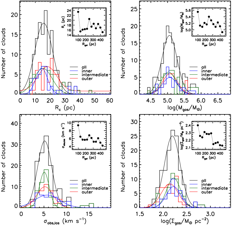
The spatially-resolved clouds of NGC4429 have sizes ranging from to about pc (see Fig. 4, top-left panel). A Gaussian fit to the size distribution yields a mean of pc and a standard deviation of pc. The clouds in NGC4429 appear to have sizes smaller than those of clouds in the MW disc (typical sizes – pc; Miville-Deschênes et al. 2017b), Local Group galaxies (typical sizes – pc; Rosolowsky et al. 2003; Rosolowsky 2007; Rosolowsky et al. 2007; Hirota et al. 2011) and most late-type galaxies (typical sizes – pc; Donovan Meyer et al. 2012; Hughes et al. 2013; Rebolledo et al. 2015), but slightly larger than those of clouds in the Galactic Centre (typical sizes – pc; Oka et al. 2001; Kauffmann et al. 2017) and the ETG NGC4526 (typical sizes – pc; Utomo et al. 2015). We note however that the CO transition used in our work traces the warm molecular medium ( K) around active SF regions, and has a higher characteristic density than the transition ( versus cm-3). The CO(3-2) line could therefore potentially trace more compact structures than CO(1-0) (Miville-Deschenes et al., 2017a; Colombo et al., 2018). The inset in the top-left panel presents the median cloud size as a function of galactocentric distance. We note that the three innermost resolved clouds (clouds No. 32, 165 and 183; pc), that all lie along the major axis, have exceptionally large masses and/or surface densities. Except for these three innermost resolved clouds, the clouds in the inner region generally have slightly smaller sizes than the clouds at larger radii (i.e. in the intermediate and outer regions). The sizes of the clouds appear to slightly increase with galactocentric distance but drop at the outer edge of the molecular disc ( pc).
The gaseous masses of the spatially-resolved clouds of NGC4429 range from to (see Fig. 4, top-right panel). The median cloud gaseous mass of the sample is . More than one third () of the resolved clouds are light ( ), but they overall contribute only of the total molecular gas mass in clouds. There is no cloud more massive than in NGC4429. The clouds in NGC4429 have gaseous masses slightly smaller than those of clouds in the MW disc ( – ; Rice et al. 2016), NGC4826 ( – ; Rosolowsky & Blitz 2005), NGC1068 ( – ; Tosaki et al. 2017), M51 ( – ; Colombo et al. 2014), NGC253 ( – ; Leroy et al. 2015) and the LMC ( – ; Hughes et al. 2010), but similar to those of clouds in M31 ( – ; Rosolowsky 2007), M33 ( – ; Rosolowsky et al. 2003, 2007), the SMC ( – ; Muller et al. 2010) and the ETG NGC4526 ( – ; Utomo et al. 2015). The clouds in the intermediate region tend to be more massive than the clouds in the inner and outer regions (see the inset in the top-right panel). The median cloud mass also appears to drop abruptly in the outermost region of the molecular disc ( pc).
The spatially-resolved clouds of NGC4429 have observed velocity dispersions (linewidths) between and (see Fig. 4, bottom-left panel). A Gaussian fit to the velocity dispersion distribution yields a mean of . The clouds in NGC4429 have observed velocity dispersions higher than those of clouds with the same sizes in the MW and Local Group galaxies (where is typically – ; Rosolowsky et al. 2003; Rosolowsky 2007; Rosolowsky et al. 2007; Fukui et al. 2008; Muller et al. 2010), but similar to those of the clouds in the ETG NGC4526 ( – ; Utomo et al. 2015). Almost all clouds with high velocity dispersions ( ) are located in the inner and intermediate regions. We find a general trend of slightly decreasing velocity dispersion with galatocentric radius (see the inset in the bottom-left panel).
The gaseous mass surface densities of spatially-resolved clouds in NGC4429 have a range of – pc-2 (see Fig. 4, bottom-right panel). A Gaussian fit to the distribution of yields a mean of dex. The clouds in NGC4429 have an average gaseous mass surface density that is lower than that of the clouds in the ETG NGC4526 ( pc-2; Utomo et al. 2015), but is comparable to that of the clouds in M33 and M64 ( pc-2; Rosolowsky et al. 2003; Rosolowsky & Blitz 2005) and is larger than that of the clouds in the MW disc and the LMC ( pc-2; Lombardi et al. 2010; Heyer et al. 2009; Hughes et al. 2010; Miville-Deschênes et al. 2017b). The gaseous mass surface densities of individual clouds in NGC4429 vary by more than an order of magnitude. We find that the clouds in the inner region tend to have a slightly larger minimum gaseous mass surface density ( pc-2) than the clouds in the intermediate ( pc-2) and outer ( pc-2) region. The general trend is that the clouds at smaller radii have higher gaseous mass surface densities (see the inset in the bottom-right panel).
3.4 GMC mass spectra
The distribution of GMCs by mass is a critical diagnostic of a GMC population and provides important clues to GMC formation and destruction (Rosolowsky, 2005; Colombo et al., 2014). We choose the gaseous mass over the Viral mass to determine the mass function, because gas mass does not require assumptions about the dynamical state of the GMCs and is well defined even for spatially-unresolved clouds. We fit the cumulative mass distribution (see Fig. 5) instead of the differential mass distribution, as Rosolowsky (2005) argues that the former is more reliable than the latter as it is not affected by biases related to binning and it can account for uncertainties of the cloud masses.
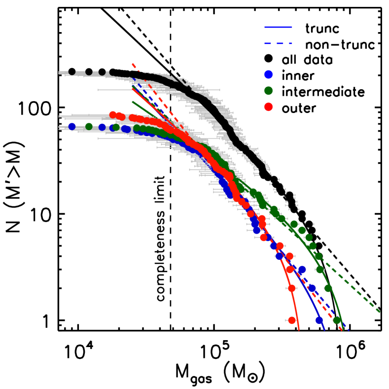
Cumulative mass distribution functions can be characterised quantitatively by a power-law function
| (8) |
where is the number of clouds with a mass greater than , sets the normalisation, and is the power-law index. Alternatively, a truncated power-law function can be used,
| (9) |
where is now the cut-off mass of the distribution and is the number of clouds with a mass , the cut-off point of the distribution (for a meaningful truncation to exist, one expects ).
We fit the cumulative mass spectra by applying the “error in variables” method developed by Rosolowsky (2005), that adopts an iterative maximum-likelihood approach to estimate the best-fitting parameters and account for uncertainties of both the cloud mass and the number distribution. Fitting is only performed above the completeness limit of , shown as a black vertical dashed line in Fig. 5. We estimate the mass completeness limit based on the minimum spatially-resolved cloud (gaseous) mass () and the observational sensitivity, i.e. , where the contribution to the mass due to noise, , is estimated by multiplying our RMS column density sensitivity limit of pc-2 by the synthesised beam area of pc2. The parameters of the best-fitting truncated power laws to the cumulative (gaseous) mass distributions of the clouds in NGC4429 are listed in Table 2.
| Region | Distance | |||
|---|---|---|---|---|
| (pc) | ( M⊙) | |||
| All | ||||
| Inner | ||||
| Intermediate | ||||
| Outer |
Notes. – All uncertainties are quoted at the level.
We find strong evidence for a curtailment of very massive GMCs in NGC4429, as a truncated power-law function (black solid line in Fig. 5) with a high value of () fits the gaseous mass distribution much better than a pure power-law function (black dashed line). This implies that NGC4429 lacks the processes that actively accumulate molecular gas clumps into high-mass GMCs. The best truncated fit yields a slope , a slope steeper than implying that most of the molecular gas mass of NGC4429 is in low-mass clouds and there should thus be a significant amount of gas below our completeness limit. This is consistent with the fact that only of the emission is decomposed into clouds at our resolution (see Section 3.2). However, there must also be a lower gaseous mass limit for the molecular clouds or a turnover at low mass for the total mass to remain finite.
Our derived slope is similar to that measured for the clouds in in the outer Galaxy (; Rice et al. 2016), the ETG NGC4526 (; Utomo et al. 2015), M51 (; Colombo et al. 2014) and the outer regions of M33 (; Rosolowsky et al. 2007), but is steeper than that for the clouds in the inner Galaxy (; Rice et al. 2016), the spiral arms of M51 (; Colombo et al. 2014), NGC1068 (; Tosaki et al. 2017), the inner regions of M33 (; Rosolowsky et al. 2007), NGC300 (; Faesi et al. 2016) and the overall mass spectrum of Local Group galaxies (; Blitz et al. 2007).
The best-fitting cut-off gaseous mass of our truncated distribution ( ) is comparable to that for the clouds in the outer Galaxy ( ; Rice et al. 2016) and the inner regions of M33 ( ; Rosolowsky et al. 2007), but is much lower than that for the clouds in most other galaxies such as the inner Galaxy ( ; Rice et al. 2016), the ETG NGC4526 ( ; Utomo et al. 2015), M51 ( ; Colombo et al. 2014), NGC1068 ( ; Tosaki et al. 2017) and the outer regions of M33 ( ; Rosolowsky et al. 2007).
Variations of the GMC gaseous mass distribution as a function of galactocentric distance can also be quantified. We find the cloud cumulative gaseous mass functions of the three regions to be slightly different, with a best-fitting truncated slope of , and and a cut-off gaseous mass of , and in the inner, intermediate and outer region, respectively. The distributions of the clouds in the inner and outer regions appear to be similar at gaseous masses below , but the latter shows a truncation while the former seems to be better fit by a pure power law even at the high-mass end. Massive clouds appear to be suppressed at the galaxy centre and especially in the outer regions of the disc. Indeed, the distribution of clouds with gaseous masses greater than the completeness limit cuts off abruptly inside pc and beyond pc (see Fig. 3). More than half of the most massive clouds ( ) are located in the intermediate region, implying that the survival of massive clouds is more favoured in this region. Overall, the environmental dependence of the gaseous mass spectrum indicates that the formation and destruction mechanisms of GMCs are (slightly) different at different galactocentric distances.
4 Cloud Kinematics
4.1 Velocity gradients of individual clouds
We observe strong velocity gradients within individual GMCs. Many authors argue that these gradients are the signature of cloud rotation (e.g. Blitz, 1993; Phillips, 1999; Rosolowsky et al., 2003; Rosolowsky, 2007; Utomo et al., 2015). The observed velocity gradient of each cloud can be quantified by fitting a plane to its intensity-weighted first moment (i.e. mean line-of-sight velocity) map :
| (10) |
where and are the projected velocity gradient along respectively the - and the -axis on the sky (selected here in the standard/intuitive manner, i.e. respectively reversely proportional to the right ascension and proportional to the declination). We adopt the code lts_planefit to perform the fits. This code combines least-trimmed-squares robust techniques (Rousseeuw & Driessen, 2006) into a least-squares fitting algorithm, and allows for intrinsic scatter, uncertainties, possible large outliers and weighting of each pixel by its flux (i.e. gaseous mass surface density). The projected angular velocity (i.e. the magnitude of the projected velocity gradient) and position angle of the rotation axis are then given by the best-fitting coefficients:
| (11) | |||
| (12) |
The uncertainties of and are estimated from the uncertainties of the parameters and using standard error propagation rules. We note that these derived projected angular velocities are underestimated by a factor compared to the intrinsic ones (i.e. ), where is the angle between the cloud rotation axis and the plane of the sky. This is however inconsequential for all following analyses and discussions, as all modelled quantities will themselves be projected onto the sky (according to the model assumptions) before comparison.
Fitting a plane to the mean line-of-sight velocity map of each cloud implicitly assumes cloud solid-body rotation. While this may not be intrinsically true (i.e. the angular velocity may depend on the radius within each cloud), because our clouds are generally relatively poorly spatially resolved, as defined above nevertheless provides a useful single quantity to quantify the bulk (projected) rotation of each cloud.
Figure 6 provides one example of our plane fitting to the mean line-of-sight velocity map of a cloud of NGC4429. The left panel shows the intensity-weighted first moment map with the best-fitting rotation axis (black line) and centre (black solid circle) overplotted. For illustrative purposes only, the right panel shows the mean velocity of each pixel within the cloud () against the perpendicular distance of the pixel from the best-fitting cloud rotation axis. A cloud with solid-body rotation should have all its data points well fit by a straight line, as is the case here. Overall, we find that planes are reasonable fits to the velocity maps of most of the clouds in NGC4429, and the median value of the reduced for the spatially-resolved clouds is . More than half () of the resolved clouds are well-fit by solid-body rotation ().
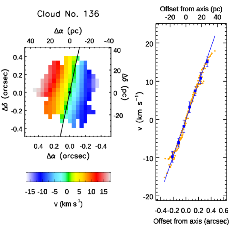
The best-fitting results are listed in Table 1. The projected velocity gradients of the spatially-resolved clouds range from to pc-1, with an average of pc-1. Our derived velocity gradients are significantly larger than those inferred for MW clouds ( pc-1; Blitz 1993; Phillips 1999; Imara & Blitz 2011), M33 ( pc-1; Rosolowsky et al. 2003; Imara et al. 2011) and M31 ( – pc-1; Rosolowsky 2007), but they are comparable to those inferred for the clouds of the ETG NGC4526 ( – pc-1; Utomo et al. 2015).
4.2 Origin of the clouds’ velocity gradients
The observed velocity gradients of the clouds can arise from turbulent motions, the clouds’ intrinsic rotation and/or galaxy rotation. Burkert & Bodenheimer (2000) suggested that turbulent velocity fields can produce observed linear gradients, that were estimated to be of order for their median cloud radius of pc. As our measured (i.e. projected) velocity gradients are generally much larger than this, we suggest turbulence is not important to account for them.
The observed velocity gradients of the clouds in NGC4429 are more likely produced by the intrinsic rotation of the clouds and/or galaxy rotation. Galaxy rotation can produce velocity gradients across the small areas occupied by GMCs, especially at small galactocentric distances corresponding to the steep part of the rotation curve. To identify the origin of the observed velocity gradients of the clouds of NGC4429, we overplot the rotation axes of the individual clouds (i.e. the projected directions of their angular momentum vectors) on the isovelocity contours of the galaxy in Fig. 7. If the velocity gradients of the clouds are produced by the clouds’ intrinsic rotation, their rotation axes should be randomly distributed. On the other hand, if the velocity gradients of the clouds are produced by the galaxy rotation, their rotation axes should show a strong alignment with the galaxy isovelocity contours.
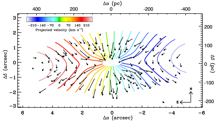
As shown in Fig. 7, we do find a strong tendency for the projected angular momentum vectors of the clouds to be tangential to the isovelocity contours of NGC4429, implying that the observed velocity gradients of the clouds are primarily a consequence of galactic rotation. This is similar to the trend in NGC4526 (Utomo et al., 2015), but different from that in the MW (Koda et al., 2006) and M31 (Rosolowsky, 2007), where the distributions of position angles are random.
Here the isovelocity contours due to the galaxy rotation were derived by creating a gas dynamical model using the Kinematic Molecular Simulation (KinMS) package of Davis et al. (2013). Inputs to the model include the stellar mass distribution, stellar mass-to-light ratio, SMBH mass, as well as the disc orientation (position angle and inclination) and position (spatially and spectrally). The stellar mass distribution is parametrised by a multi-Gaussian expansion (MGE; Emsellem et al. 1994) fit to a -band image from HST (Davis et al., 2018). The free parameters are derived by fitting to the observed gas kinematics, assuming the object is axisymmetric (in the central parts where CO is located) and the gas in circular rotation (see Davis et al. 2018 for details of the fitting procedures and the best-fitting parameters). The dark matter and gas masses are not included in our model, as they are small compared to those of the SMBH and stars. We note that a variable mass-to-light ratio has been adopted, as required by the data, with a piecewise linear form as a function of radius. An inclination angle of and a kinematic position angle of (as measured in that work) are adopted to calculate the line-of-sight projection of the gas circular velocities.
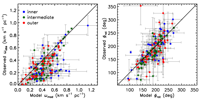
To further quantify the effects of the galaxy rotation on our observed velocity gradients, we compare the measured angular velocities and position angles of the rotation axes of the clouds in NGC4429 to those expected from a pure galaxy rotation model. We measure the projected angular velocities and rotation axes of the model over the same areas as for the observed clouds, using the methods described in Section 4.1. We assume that the motion of the gas within each cloud (i.e. each fluid element of each cloud) follows perfectly circular orbits defined by our kinetic model above. We find a strong correlation between the modelled and observed position angles (with a median angle difference of ), supporting the idea that the observed cloud-scale velocity gradients are aligned with the large-scale velocity field, as suggested by Fig. 7.
A general correlation between the modelled and observed angular velocities is also found. Our model overestimates the observed angular velocities by a median factor of , much smaller than the ratios found for clouds in WISDOM late-type galaxies (; Shu et al., in prep; Choi et al., in prep). This discrepancy between the amplitudes of the observed and modelled angular velocities is unlikely to be due to the clouds’ own rotations, as the observed position angles of the clouds would then be expected to deviate from the modelled ones randomly. A possible explanation is that the self-gravity of the clouds is also important, so that the clouds do not follow pure galaxy rotation (see Section 6.2 for more discussion of this). The discrepancy could also partly be due to the limitation of CPROPS to isolate individual clouds in highly-crowded environments. To reduce the ambiguities due to cloud blending, we fit both the data and model again without including the outermost boundary pixels of each cloud. In this case, a strong correlation between the modelled and observed position angles is again present (see the right panel of Fig. 8), with a median angle difference of , but the model overestimates the observed angular velocities by a reduced median factor of only (left panel of Fig. 8). In the inner region, where the clouds are more blended in both space and velocity, the discrepancies between the modelled and observed angular velocities is worse (with a median factor of ), and the angle difference is larger (with a median value of ). In the outer region, where clouds are less blended, the model shows a much better agreement with the observations (with a median angular velocity discrepancy factor of only and a median angle difference of only )
In summary, a comparison of the observed and modelled projected angular velocities and rotation axes of individual clouds suggests that the observed velocity gradients of the clouds in NGC4429 are primarily caused by the local circular orbital motions, themselves due to the galaxy potential. We note that the good match between our observations and model suggests that the motion of the gas within each cloud of NGC4429 mainly follows gravitational orbital (and thus shear) motions rather than epicyclic motions (see Section 6.1 for more discussion of this issue).
5 Dynamical State of Clouds
5.1 Cloud scaling relations using the observed velocity dispersion
The scaling relations between the physical properties of molecular clouds have become a standard tool for assessing the clouds’ physical states and dynamical conditions (e.g. Blitz et al., 2007; Hughes et al., 2013). The most fundamental relation is the size – linewidth relation, a.k.a. Larson’s first relation (e.g. Larson, 1981; Solomon et al., 1987), that has become the yardstick for GMC studies in the MW and external galaxies (e.g. Bolatto et al., 2008). The size – linewidth relationship is usually interpreted as a signature of the turbulent motions within clouds (e.g. Falgarone et al., 1991; Elmegreen & Falgarone, 1996; Lequeux, 2005), and it provides a unique probe of the dynamical state of the turbulent molecular gas in extragalactic star-forming systems.
Another important scaling relation providing crucial insights is the correlation between the clouds’ dynamical (i.e. Virial) masses and their true masses (here taken to be the gaseous masses ). The comparison of the Virial and gaseous masses provides an important clue to the dynamical state of the clouds according to the Virial theorem. Indeed, the Virial parameter
| (13) |
(see Eq. 7) is equal to the ratio of two times the turbulent kinetic energy to the (absolute value of the) self-gravitational energy of a cloud, quantifying the degree of gravitational boundedness of the cloud. If the Virial parameter of a cloud , the cloud is gravitationally bound and in Virial equilibrium. If its Virial mass is much larger than its gaseous mass (), the cloud has to be confined by external pressure (it would otherwise disperse) and it is unlikely to be bound (i.e. it is a transient feature of the ISM). If , the molecular cloud is likely unstable to gravitational collapse. We note that a critical parameter is often regarded as the threshold between gravitationally-bound and unbound objects (Kauffmann et al., 2013; Kauffmann et al., 2017).
A third important scaling relation is the correlation between the clouds’ mass surface densities (again taken here to be the gaseous mass surface densities ) and the quantities (where as before and are a measure of the observed/1D velocity dispersion and size of each cloud, respectively). The – plot provides a necessary modification to Larson’s scaling relations. It implies an additional constraint to the velocity dispersion, whereby the velocity dispersion of a cloud depends on both its spatial extent and its gaseous mass surface density (Field et al., 2011). If clouds are virialised (and do not necessarily obey Larson’s first relation), observations should cluster around the line ( for a homogeneous spherical cloud; see the black solid diagonal line in the right panel of e.g. Fig. 9). If clouds are not virialised but are marginally gravitationally bound (i.e. ), the data points should cluster around the line (see the black dotted diagonal line in the right panel of e.g. Fig. 9). If clouds are not gravitationally bound, external pressure () must play an important role to confine the clouds, and the clouds should be distributed along the black V-shaped dashed curves in the right panel of Fig. 9: (Field et al., 2011). We note that for the largest of each V-shaped curve, the clouds are dominated by self-gravity and the equilibrium curve is asymptotic to the solution of the simple Virial equilibrium (SVE, i.e. the black solid diagonal line; Field et al. 2011).
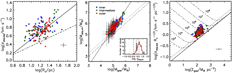
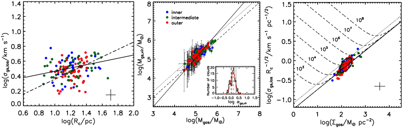
For consistency with GMC studies in the MW and external galaxies in the literature, we first adopt the observed velocity dispersion (see Section 3.1) to explore the above three scaling relations. As seen in the left panel of Fig. 9 (data points and black solid line), there is a strong correlation between size and linewidth (with a Spearman rank correlation coefficient of ) for the clouds of NGC4429 that are spatially resolved, the only clouds where a reliable measurement of the size is possible (see Table 1). However, the relation departs from the traditional one derived for clouds in the MW disc (black dashed line in the left panel of Fig. 9; Solomon et al. 1987; Dame et al. 2001; Rice et al. 2016). The observed tendency is for clouds to exhibit a higher velocity dispersion at a given size. Our results also reveal a steep size – linewidth relation,
| (14) |
steeper than that of clouds in the MW disc (; Solomon et al. 1987). The slope is also marginally steeper than that derived for CMZ clouds (; Kauffmann et al. 2017), but the zero-point is much smaller ( for CMZ clouds; Kauffmann et al. 2017), and the velocity dispersions of CMZ clouds are indeed higher than those of the NGC4429 clouds at any given size.
The Virial masses of the spatially-resolved clouds of NGC4429 calculated from their observed velocity dispersions,
| (15) |
(see Eq. 7), are compared to their gaseous masses in the middle panel of Fig. 9, where as always we have assumed (spherical homogeneous clouds). We find Virial masses significantly larger than the gaseous masses. A linear fit yields (black solid line in the middle panel of Fig. 9)
| (16) |
A log-normal fit to the distribution of the resulting Virial parameters,
| (17) |
shown as an inset in the middle panel of Fig. 9, yields a mean and a standard deviation of dex. In particular, all resolved clouds have .
The derived relation is presented in the right panel of Fig. 9 for the spatially-resolved clouds of NGC4429. The gaseous mass surface densities of the GMCs vary by one order of magnitude, and the size – linewidth coefficient () increases with increasing . The data points do not lie along the solid diagonal line of the SVE, but are instead offset from it and distributed across the -shaped curves. If pressure is important to the dynamical state of the clouds, the clouds in NGC4429 seem to experience a wide range of considerable external pressures ( – K cm-3, where is Boltzmann’s constant). Overall, Fig. 9 thus seems to suggest that the kinetic energy of the clouds in NGC4429 is more important than their gravitational energy, hence the clouds are either not bound or tend toward pressure equilibria.
However, a major concern about the use of the above relations to assess the dynamical states of clouds in NGC4429 is the applicability of the observed velocity dispersion . The difference of the derived size – linewidth relation with respect to the Solomon et al. (1987) trend seems to imply that the measured linewidths of the clouds are not set purely by their internal virialised motions and/or turbulence (Meidt et al., 2013; Kauffmann et al., 2017). Recent works suggest that, in the centre of galaxies where strong shear and tidal forces are present, a considerable part of the cloud-scale gas motions is due to these external galactic forces (e.g. Meidt et al., 2018; Utreras et al., 2020). We have already demonstrated that the observed strong velocity gradients of the clouds in NGC4429, that reflect the velocity gradients in the plane of the galaxy, are mainly a consequence of local orbital motions defined by the background galactic gravitational potential (i.e. the galaxy circular velocity curve; see Section 4.2). In this case, the steep slope of the size – linewidth relation (see the left panel of Fig. 9) can be explained as resulting from the decay of fast orbit-induced large-scale motions to transonic conditions on small spatial scales (Kauffmann et al., 2017).
The question then is whether gas motions associated with the background galactic potential should also be involved in assessing the dynamical states and stability of the clouds. Intuitively, gas motions due to external galactic forces should be considered when calculating a cloud’s kinetic energy that is meant to balance its self-gravitational energy (Chen et al., 2016; Meidt et al., 2018). Conversely, in the presence of strong galactic forces, self-gravity is no longer the only force binding a cloud. Therefore, to verify whether clouds are virialised in a galactic environment where tidal/shear forces are strong, one needs to modify the conventional Virial theorem to include (1) external forces arising from the background galactic potential and (2) the gas motions induced by these forces. We do exactly that in the next sub-sections.
5.2 Basic framework
We recall here a key conceptual point emphasised in Section 1. We will not assume here that the clouds of NGC4429 are in dynamical equilibrium, and then deduce the clouds’ gravitational motions due to the external (i.e. galactic) potential. Rather, we will measure and quantify the clouds’ gravitational motions due to the external potential, and then deduce whether the clouds are indeed in dynamical equilibrium. This is the only way to reliably assess whether GMCs are in dynamical equilibrium (and thus long-lived) or out of equilibrium (and thus transient), arguably the most important question in the field.
As described in detail in Appendix A, we envision each cloud as a continuous structure with well-defined borders in position- and velocity-space, located in a rotating gas disc with a circular velocity determined by the shape of the background galactic gravitational potential. Each cloud’s centre of mass (CoM) is assumed to be in the mid-plane of the disc. We assume that each fluid element of a cloud experiences two kinds of motions: (1) random turbulent motions arising from self-gravity (cloud gravitational potential ), that have a velocity dispersion , and (2) bulk gravitational motions associated with the external (i.e. galactic) potential (), that have a RMS velocity (, where is the velocity of each fluid element due to gravitational motions relative to the CoM, the integral is over all fluid elements , and ). Thermal motions are ignored, as they are often small compared to turbulent motions in a cold gas cloud (e.g. Fleck, 1980). We assume the motions due to self-gravity () and the background galactic potential () to be uncorrelated, and the cloud’s own gravitational potential to be (statistically) independent of the local external gravitational potential defined by the galaxy . The turbulent motions due to self-gravity are expected to be quasi-isotropic in three dimensions (Field et al., 2008; Ballesteros-Paredes et al., 2011), while the gas motions induced by the external gravitational potential are often non-isotropic (Meidt et al., 2018). Gravitational motions in the plane are assumed to be separable from those in the vertical direction. We consider only the effects of gravitational forces and ignore external pressure and magnetic fields.
With those considerations, the resulting modified Virial theorem (MVT) can be split into two independent parts:
| (18) |
where , , and are respectively the cloud’s moment of inertia, mass, radius and scale height, (formally the total mass volume density evaluated at the cloud’s CoM, but we use here , the stellar mass volume density evaluated at the cloud’s CoM using our MGE model, as it is accurately constrained; see Appendix C), is the aforementioned geometrical factor that quantifies the effects of inhomogeneities and/or non-sphericity associated with self-gravity, is a geometrical factor that quantifies the effects of inhomogeneities (only) associated with external gravity ( for a spherical cloud with a radial mass volume density profile , thus for a spherical homogeneous cloud as before; see Appendix A for more details on ), is the cloud’s 1D turbulent velocity dispersion due to self-gravity, , and are the RMS velocity of gas motions due to external gravity in respectively the radial (i.e. the direction pointing from the galaxy centre to the cloud’s CoM), azimuthal (i.e. the direction along the orbital rotation) and vertical (i.e. the direction perpendicular to the cloud’s orbital plane) direction (as measured in an inertial frame, i.e. by a distant observer; see Appendix A for a more detailed discussion of and ), is the circular orbital angular velocity at the cloud’s CoM, and is the tidal acceleration per unit length in the radial direction (e.g. Stark & Blitz, 1978) evaluated at the cloud’s CoM ( is the galactocentric distance in the plane of the disc and that of the cloud’s CoM). We note that here and throughout, is the theoretical quantity defined by the galaxy potential , i.e. it is the angular velocity of a fluid element moving in perfect circular motion (, where is the circular velocity curve) rather than the observed angular velocity of the fluid element (, where is the observed rotation curve). The first term in square brackets on the right-hand side (RHS) of Eq. 18 comprises the energy terms regulated by self-gravity, while the second term in square brackets contains the contributions of external gravity to the cloud’s energy budget () in respectively the vertical direction () and the plane (). The detailed derivation of Eq. 18 and its more general form for a homogeneous ellipsoidal cloud (Eq. 81) is provided in Appendix A.
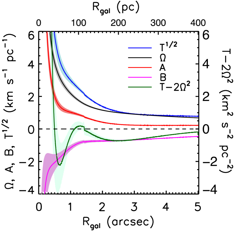
For reference, we show in Fig. 10 the dependence of , Oort’s constants and , and on galactocentric distance in NGC4429. The functions , and are always positive, is always negative, while is generally negative except in the very centre. We note that . The rotational shear (i.e. Oort’s constant ) in NGC4429 is much larger ( at galactocentric distances pc, where the clouds are located) than that in the bulk of the Galactic disc ( at kpc; Dib et al. 2012) and the LMC ( at kpc; Thilliez et al. 2014).
5.3 Role of self-gravity
The first term in square brackets on the RHS of Eq. 18 describes an internal equilibrium regulated by self-gravity. For a cloud that attains Virial balance between its internal turbulent kinetic energy () and its self-gravitational energy (), such as an isolated self-gravitating cloud, these two terms should cancel out. To investigate the role of self-gravity, one thus needs to measure the cloud’s turbulent velocity dispersion due to self-gravity only (). However, the observed velocity dispersion is not necessarily equal to , as there are potentially significant contributions from bulk (galaxy-driven) gravitational motions. Indeed, the observed velocity dispersion of a cloud can be expressed as
| (19) |
where is the inclination of the galactic disc with respect to the line of sight, and is the (deprojected) azimuthal angle of the cloud’s CoM with respect to the kinematic major axis of the disc (see Eq. 32 of Meidt et al. 2018).
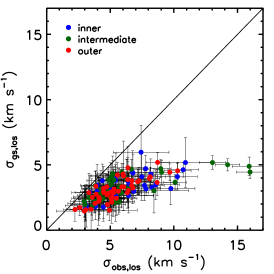
We therefore need to reduce the contamination of our measured velocity dispersions by bulk gravitational motions. This is why we introduced a new measure of the velocity dispersion, , in Section 3.1, where we first shifted each line-of-sight velocity spectrum to match its centroid velocity () to that of the cloud’s CoM (), and then measured the velocity dispersion (i.e. the second moment along the velocity axis) of the shifted emission distribution and extrapolated it to K. The derived gradient-subtracted velocity dispersion was then deconvolved by the channel width (), yielding our final adopted measure. Table 1 lists the derived of all spatially-resolved clouds and the left panel of Fig. 11 shows a comparison of and . As expected, , and all particularly large measurements have been corrected to .

The observed velocity gradient of a cloud is due to bulk motions within the cloud only. Assuming that the vertical gravitational motions can be treated as random motions that balance the weight of the disc (i.e. no bulk motion in the vertical direction), analogously to turbulent motions due to self-gravity, the only bulk motions will originate from in-plane gravitational motions. Our newly-derived gradient-subtracted velocity dispersion can therefore be written as
| (20) |
minimising contamination from bulk gas motions in the plane. Our gradient-subtracted velocity dispersion thus removed the second term (in-plane bulk gravitational motions) but kept the first term (turbulent self-gravitational motions) and last term (vertical random gravitational motions) on the RHS of Eq. 19. However, as we will demonstrate below, the term is negligible compared to in NGC4429 and can thus safely be ignored, so that in NGC4429. Using our newly derived measure, we thus revisit the scaling relations of Fig. 9 in Fig. 12.
5.4 Cloud scaling relations using the gradient-subtracted velocity dispersion
The left panel of Fig. 12 (data points and black solid line) presents the size – linewidth relation based on our measure for the spatially-resolved clouds of NGC4429. We now find the size – correlation to be rather weak, with a Spearman rank coefficient of . However, compared with the size – linewidth relation using , it appears to better follow the relation of the MW disc clouds (black dashed line in the left panel of Fig. 12). Indeed, the data points seem to cluster around the MW disc scaling law (Solomon et al., 1987), although there is a large scatter. A weak size – linewidth relation has also been inferred in other galaxies (e.g. Hughes et al., 2013; Utomo et al., 2015), but a small dynamic range and the relatively large uncertainties of our measurements probably at least partially explain the poor correlation.
We find a nearly linear correlation between the -derived Virial masses,
| (21) |
(see Eq. 7), and the CO-derived gaseous masses of the spatially-resolved clouds (black solid line in the middle panel of Fig. 12), where we have again assumed (spherical homogeneous clouds):
| (22) |
A log-normal fit to the distribution of the resulting Virial parameters,
| (23) |
shown as an inset in the middle panel of Fig. 12, yields a mean and a standard deviation of dex. No systematic variation is observed in the Virial parameter for clouds over a wide range of galactocentric distances.
The right panel of Fig. 12 shows the comparison between and the gaseous mass surface density for the spatially-resolved clouds. The data points are distributed along the black solid diagonal line, suggesting a simple Virial equilibrium. Therefore, when the contamination of in-plane bulk motions is removed, the clouds in NGC4429 do seem to reach a state of Virial equilibrium.
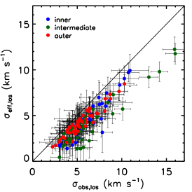
A full determination of the internal equilibrium state of clouds regulated by self-gravity (i.e. the first term in brackets on the RHS of Eq. 18) requires a knowledge of rather than . However, we can still gain important insights from Fig. 12. First, our measured should be strongly dominated by , i.e. and thus (see Eq. 20), otherwise (if were to contribute significantly to ) the scaling relations presented in Fig. 12 would depend on the galaxy’s inclination angle and the trend seen in Fig. 12 (suggesting a state of gravitational equilibrium) would turn out to be merely a coincidence. But we note that a similar result was obtained in another ETG. Indeed, NGC4526 revealed a good agreement between the -derived Virial masses and the CO-derived gaseous masses (), and similarly a – correlation as expected from Virial equilibrium (Utomo et al., 2015). We thereby consider that the most likely explanation of our results in Fig. 12 (and the results of Utomo et al. 2015) is that is dominated by (that is assumed isotropic and thus independent of the galaxy inclination angle) and that an internal gravitational equilibrium has been achieved through self-gravity. This assumption is particularly reasonable in NGC4429, as in any case only a very small part of can contribute to considering its high disc inclination ( so ).
If , then the left panel of Fig. 12 seems to suggest that the clouds’ internal turbulent motions associated with self-gravity follow the classical size – linewidth relation of MW clouds, despite a large scatter. This supports the traditional interpretation of turbulent motions as the origin of the size – line width relation (e.g. Mac Low & Klessen, 2004; Ballesteros-Paredes et al., 2006, 2007, and references therein), that emerges entirely as a consequence of the gas self-gravity (Camacho et al., 2016; Ibáñez-Mejía et al., 2016). The middle panel of Fig. 12 then implies that , i.e. that GMCs attain approximate Virial balance between their internal turbulent kinetic energies and their self-gravitational energies. The fact that the mean is slightly larger than one () may be due to contamination of by the term. Indeed, in Section 6.4 we will show that the motions induced by (external) gravity contribute around of the total . The right panel of Fig. 12 then further indicates that an internal virialisation has been roughly achieved by self-gravity. In other words, the gravitational potential defined by the mass of a cloud is matched by the kinetic energy induced by self-gravity. In this case (), we have
| (24) |
(see Eq. 7), and (where is the Virial parameter set purely by a cloud’s self-gravity), as has been suggested by many previous studies of self-gravitating clouds (e.g. Eq. 10 in Heyer et al. 2009).
We note that this internal Virial equilibrium is established by self-gravity despite the presence of an external galactic potential, which seems to support our previous assumption that the motions due to self-gravity emerge independently of the background galactic potential. For more discussion of how a Virial equilibrium is established through the balance of turbulent kinetic and self-gravitational energy, see Meidt et al. (2018).
5.5 Role of external gravity
The contribution of external gravity to a cloud’s gravitational energy budget () is given by the second term in brackets on the RHS of Eq. 18:
| (25) |
If , external gravity acts against self-gravity and makes the cloud less bound. If , external gravity acts with self-gravity and contributes to the collapse of the cloud. If , the effect of external gravity can be ignored. A more general form of for a homogeneous ellipsoidal cloud is provided in Appendix A (Eq. 79). We can split into two independent parts, one in the vertical direction () and one in the plane (), and consider them in turn.
Vertical direction. The contribution of the external potential to the gravitational energy budget of the cloud in the vertical direction is
| (26) |
It is similar to the vertical hydrostatic equilibrium equation of a gaseous disc (e.g. Eq. 3 in Koyama & Ostriker, 2009). If it is positive, the cloud will be disrupted in the vertical direction, but if it is negative, the cloud will collapse in the vertical direction. However, as neither nor can be measured directly from our observations, we can not really assess the vertical equilibrium state of the clouds. But if we make the common assumption that vertical equilibrium is satisfied on a cloud scale, i.e. that the vertical contribution of external gravity to the net energy budget of a cloud is negligible (i.e. ), then we can derive a relation between and :
| (27) |
The measured scale heights of clouds in edge-on disc galaxies can thus be used to determine their unobservable vertical velocity dispersions , or conversely the measured line-of-sight velocity dispersions of clouds in face-on galaxies can be used to determine the unobservable scale heights , as suggested by Koyama & Ostriker (2009). In our work, we can estimate the value of from the deviation of from , and then infer a cloud’s scale height (combining Eqs. 20 and 27; see Section 6.4). We note that our derived – correlation is different from the one derived via the epicyclic approximation by Meidt et al. (2018), by a factor of ( in Meidt et al., 2018). This is because we assumed a spherical cloud with a radial mass volume density distribution (i.e. ) while Meidt et al. (2018) assumed a cloud with an exponential vertical mass volume density distribution (i.e. ). Overall, to retain vertical hydrostatic equilibrium on a cloud scale, the gravitationally-induced vertical motions () need to balance the vertical weight of the background galaxy.
We note here that assuming vertical equilibrium for the clouds goes against our stated aim of inferring whether the clouds are indeed in equilibrium directly from measurements. However, galaxies are highly symmetric vertically and there is no bulk motion in the vertical direction, and we will show below that we do not need to assume the clouds are in equilibrium in the plane. We therefore keep moving forward with our plan, even if it can only be partially achieved.
Plane. The contribution of the external potential to the gravitational energy budget of a cloud in the plane is
| (28) |
The orbital angular velocity and the tidal acceleration parameter at the cloud’s CoM can be derived from our gas dynamical model (see Section 4.2 and Fig. 10) and they are listed for each cloud in Table 3. A more general form of for a homogeneous ellipsoidal cloud is provided in Appendix A (Eq. 77). The term indicates the effective potential energy of galactic gravity and the centrifugal force (see Appendix A for more details). We find that galactic gravity and the centrifugal force act as a binding force overall, as the corresponding energy is negative in all cases (the function is generally negative except in the very centre, pc, where there is no cloud; see Fig. 10). On the other hand, clouds are supported against collapse by the gravitationally-induced gas motions in the plane, whose kinetic energy is . The question then is which of the binding energy of galactic gravity plus the centrifugal force or the kinetic energy of gravitational motions is more important, i.e. whether or (or ).
| ID | ||||
| () | () | |||
| 1 | 1.26 | |||
| 2 | 1.33 | |||
| 3 | 1.34 | |||
| 4 | 1.41 | |||
| 5 | 1.47 | |||
| 6 | 1.29 | |||
| 7 | 1.26 | |||
| 8 | 1.50 | |||
| 9 | 1.39 | |||
| 10 | 1.59 | |||
| 11 | 1.27 | |||
| 12 | 1.34 | |||
| 13 | 1.52 | |||
| 14 | 1.64 | |||
| 15 | 1.43 | |||
| 16 | 1.40 | |||
| 17 | 1.50 | |||
| 18 | 1.53 | |||
| 19 | 1.18 | |||
| 20 | 1.60 | |||
| … | … | … | … | … |
| 217 | 1.21 |
Notes. – Clouds with no entry are unresolved spatially. Calculations of assume (spherical homogeneous clouds). All uncertainties are quoted at the level, and those of have been propagated from the uncertainties of both observed and modelled quantities (see Eq. 38). As noted in the text, the uncertainty of the adopted distance to NGC4429 was not propagated through the tabulated uncertainties of the quantity . This is because an error on the distance to NGC4429 translates to a systematic (rather than random) scaling of some of the measured quantities (no effect on the others), here , and in Eq. 38. Oort’s constants and can be derived using respectively and . Table 3 is available in its entirety in machine-readable form in the electronic edition.
As suggested by Eq. 28, a full derivation of requires knowledge of and , the RMS velocities of gravitationally-induced motions in the plane. Although and can not be obtained directly from observations, we can nevertheless glean some information about them from the observed quantities and . Indeed, if we assume the gas motions induced by the galactic potential to be isotropic in the plane (i.e. ), the RMS velocities of the in-plane gas motions due to external gravity can easily be derived by combining Eqs. 19 and 20:
| (29) |
Substituting Eq. 29 into Eq. 28, we find the net contribution of external gravity to the gravitational budget of the clouds in NGC4429 to be positive in most cases (i.e. ). Therefore, the main effect of the external gravity on the clouds of NGC4429 is to make them less bound (in the plane).
Effective parameters. Our MVT (Eq. 18) can be written simply as
| (30) |
(see Eq. 25). However,
| (31) |
(see Eq. 13), the traditional Virial parameter regulated by self-gravity only, and we define
| (32) |
the ratio between the contribution of external gravity and the (absolute value of the) cloud’s self-gravitational energy (), so that
| (33) |
This naturally leads us to define an effective Virial parameter
| (34) |
such that
| (35) |
Thus, just like the standard Virial parameter, this effective Virial parameter informs on the dynamical stability of a cloud. If , the cloud is gravitationally bound and in Virial equilibrium even in the presence of the external (i.e. galactic) gravitational potential. If , the cloud is unlikely to be bound (i.e. it is transient unless confined by other forces). If , the molecular cloud is likely to collapse. For clouds that are (marginally) gravitationally bound, we again require (Kauffmann et al., 2013; Kauffmann et al., 2017), or equivalently if an internal Virial equilibrium is established by self-gravity (i.e. if ; see Eq. 34).
Equivalently, from Eq. 13, we can define an effective velocity dispersion
| (36) |
and thus our modified Virial equation (Eq. 18) can be simplified to
| (37) |
The parameters (via Eq. 35) or equivalently (via Eq. 37) thus embody our MVT and offer a straightforward method to test the gravitational boundedness of a cloud in the presence of an external (i.e. galactic) gravitational field.
Of course, our expressions are of no use in practice if the external contribution can not be evaluated (see Eq. 25). Indeed, without knowledge of , and , none of , or can be evaluated. However, by making increasingly stringent assumptions, we show in Appendix B that it is possible to evaluate all these quantities from observable quantities alone. We thus briefly summarise those assumptions and their consequences here, but refer to Appendix B for detailed calculations.
First, we assume clouds are in vertical hydrostatic equilibria, i.e. (Eq. 27), so that the contribution of the external potential to the gravitational energy budget of each cloud in the vertical direction vanishes, i.e. (see Eq. 26). Second, we assume the motions associated with external gravity to be isotropic in the plane, i.e. (Eq. 29). Third, we assume (or equivalenty ; see Eq. 20) and thus . As shown in Appendix B, all three assumptions taken together lead to
| (38) |
(see Eqs. 25, 36, 34, 23 21 and 32). More general forms for a homogeneous ellipsoidal cloud are provided in Appendix B. These Eqs. 38 represent our final MVT, whose power lies in the fact that all of , and can be evaluated directly from observations. Indeed, as mentioned previously, the measured (), , and are listed for each spatially-resolved cloud in Table 1, while , and the resulting (and thus ; see Eq. 36) are listed in Table 3.
The first term on the RHS of Eqs. 38 (except for ) comprises the gas turbulent motions associated with a cloud’s self-gravity, the second term denotes the gravitational motions associated with external gravity in the plane, and the last term encompasses the external/galactic forces on the cloud.
An extended Virial theorem including the background tidal field was formulated by Chen et al. (2016), but they only evaluated two representative cases, namely a non-rotating cloud (; Eq. 17 in their paper) and a tidally-locked cloud (; Eq. 18 in their paper). Our derived MVT is valid for more general cases. In fact, we obtain the same results as Chen et al. (2016) for their two particular cases. For a non-rotating cloud, , and we derive . For a tidally-locked cloud (i.e. Oort’s constants and ), (as ; see Eq. 128 in Appendix B), and we derive . We note that the velocity dispersion used by the extended Virial theorem of Chen et al. (2016) should be the internal turbulent velocity dispersion rather than the observed (i.e. total) velocity dispersion.
Overall, to take into account the influence of external gravity on the dynamical state of a cloud, one should use the effective virial parameter and effective velocity dispersion . The latter quantifies the net kinetic energy that balances the cloud’s (self-)gravitational potential energy. The kinetic energy obtained using includes the cloud’s internal turbulent kinetic energy due to self-gravity as well as the contributions from the external gravity. If or , external gravity acts against self-gravity and makes the cloud less bound (i.e. ). If or , external gravity acts with self-gravity and contributes to the cloud’s confinement and/or collapse (i.e. ). If or , then external gravity has no effects on the cloud’s dynamical state (i.e. ). Therefore, the results presented in Figs. 9 and 12, that respectively adopt and , do not reflect the real dynamical states of the NGC4429 clouds. Specifically, embodies gas motions associated with self-gravity and external gravity, but it ignores the extra binding energy provided by galactic forces and the centrifugal force (i.e. the term in Eqs. 18, 25 and 28, that is negative in almost all cases), so it overestimates the effect of external gravity on the clouds. Conversely, only reflects gas motions associated with self-gravity, so it does not include the contribution of external gravity to a cloud’s gravitational energy budget.
5.6 Cloud scaling relations using the effective velocity dispersion
In consequence, we revisit yet again the three scaling relations that describe the dynamical states of the clouds in NGC4429, this time using the effective velocity dispersion defined in Eqs. 38. In most cases our derived is larger than the gradient-subtracted velocity dispersion , and in all cases it is smaller than the observed velocity dispersion (see Fig. 11). This implies that external gravity generally makes the clouds less bound. We nevertheless note that we find a few clouds where is smaller than , suggesting external gravity contributes to the cloud’s confinement and/or collapse in these few cases. As expected in Eq. 38, these clouds all have nearly equal to , and thus low velocity gradients of .
The left panel of Fig. 13 (data points and black solid line) presents the – relation for the spatially-resolved clouds of NGC4429, where we have assumed (homogeneous clouds). The relation appears to have a slightly steeper slope () than that of MW clouds (; Solomon et al. 1987), but the correlation is very weak (with a Spearman rank correlation coefficient of ).
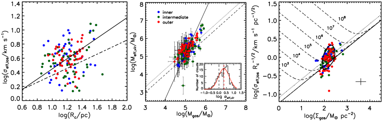
The Virial masses of the spatially-resolved clouds derived using , referred to as effective Virial masses
| (39) |
(see Eq. 7), are compared to the CO-derived gaseous masses in the middle panel of Fig. 13, where we have again assumed (spherical homogeneous clouds). A linear fit between effective Virial and gaseous mass yields (black solid line in the middle panel of Fig. 13)
| (40) |
A log-normal fit to the distribution of the resulting effective Virial parameters,
| (41) |
(see also Eq. 36), shown in the first panel of Fig. 14, yields a mean and a standard deviation of dex. This mean is higher than (see Section 5.4), suggesting that the main effect of external gravity on the clouds is to make them less bound. However, since many NGC4429 clouds have a mean effective virial parameter close to the critical value regarded as the boundary between gravitationally-bound and unbound clouds (Kauffmann et al., 2013; Kauffmann et al., 2017), i.e. , the clouds should still be marginally gravitationally bound.
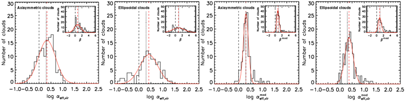
The inset in the first panel of Fig. 14 shows the distribution of the measured (Eq. 32). A Gaussian fit yields a mean and a standard deviation of . Given these , the contribution of external gravity to each clouds’ energy budget is generally significant, on average of the order of (and frequently exceeding) the self-gravitational energy (see also Eq. 34). We will discuss this aspect further in Section 6.2. However, we note immediately that a noticeable fraction of spatially-resolved clouds ( or ) have . These negative could be due to observational uncertainties, and thus inaccuracies when estimating (or ), but some clouds may well have their gas motions decoupled from global galaxy rotation. Indeed, we found that clouds with have larger discrepancies between their observed and modelled angular momenta (with a median projected angular velocity discrepancy factor of and a median position angle difference of ; see Section 4.2) than clouds with (with a median projected angular velocity discrepancy factor of and a median position angle difference of ). It thus seems that clouds with only weakly follow the galaxy orbital rotation. These clouds are therefore presumably not as strongly affected by galactic shear and tidal forces, and they can become more virialised (with ).
The right panel of Fig. 13 shows the – relation for the spatially-resolved clouds of NGC4429. The data points are mostly distributed away from the black solid diagonal line (SVE), but they are clustered around the black dotted diagonal line. This again suggests that, although the NGC4429 clouds are not virialised, they could be marginally gravitationally bound.
5.7 Cloud scaling relations considering ellipsoidal clouds
By using a single measure of size for each cloud (; see Section 3.1), our analysis has so far implicitly assumed that each cloud is axisymmetric in the orbital plane. However, the effects of external gravity on a cloud (and its contribution to a cloud’s energy budget) also formally depend on the actual shape and position angle of the cloud (see Appendices A and B). To assess the impacts of this assumption, we now assume instead that each cloud has an ellipsoidal geometry, with semi-axis perpendicular to the orbital plane and semi-major axis (at a position angle with respect to the radial/galactocentric direction) and semi-minor axis in the orbital plane.
If an ellipsoidal cloud is homogeneous, Appendices A and B show that Eqs. 38 (that assume vertical equilibrium, isotropy in the equatorial plane and ) become
| (42) |
These equations thus represent our final MVT (Eqs. 38) for the case of a homogenous ellipsoidal cloud.
We note that , and in Eqs. 42 should be measured in the cloud’s orbital plane (i.e. the galaxy’s equatorial plane) rather than the sky plane. To correct for the effects of inclination, we thus create an image of each cloud deprojected to a face-on view, from which we measure the semi-major and semi-minor axes analogously to in Section 3.1 and the position angle with respect to the radial/galactocentric direction.
The left panel of Fig. 15 presents the – relation for the spatially-resolved clouds of NGC4429 assuming they are ellipsoidal and (homogeneous clouds). The relation has a slope of , consistent with that of axisymmetric clouds (; see Section 5.6), and is thus again slightly steeper than that of MW clouds (; Solomon et al. 1987), although the correlation is again very weak (with a Spearman rank correlation coefficient of 0.09.
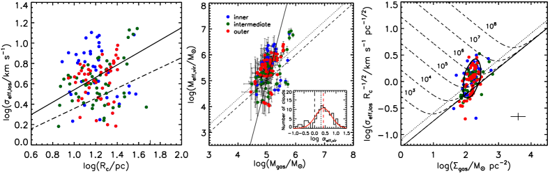
The effective Virial masses of the spatially-resolved clouds () derived assuming ellipsoidal shapes (see Eq. 7;where is defined as ) are compared to the CO-derived gaseous masses in the middle panel of Fig. 15. We have again assumed (homogeneous clouds), but calculated , that quantifies the effects of the ellipticity, separately for each cloud using the method provided by Bertoldi & McKee (1992) (see Appendix A for more details). We find the exact cloud morphology has negligible effects on the quantities regarding to the cloud’s self-gravity (e.g. and ), as is approximately unity (). A linear fit between the effective Virial and gaseous masses (black solid line in the middle panel of Fig. 15) yields a slope of . A log-normal fit to the distribution of the effective Virial parameters () derived assuming ellpsoidal clouds (see Eqs. 41 and 42), shown in the second panel of Fig. 14, yields a mean and a standard deviation of dex, only slightly larger than that estimated assuming axisymmetric clouds (; see Section 5.6), and again higher than (see Section 5.4), suggesting that the main effect of external gravity on the clouds is to make them less bound irrespective of their exact shapes.
The inset in the second panel of Fig. 14 shows the distribution of the resulting for the spatially-resolved clouds of NGC4429, calculated assuming ellipsoidal clouds. A Gaussian fit to the distribution yields a mean and a standard deviation of , again slightly larger than that derived assuming axisymmetric clouds (; see the first panel of Fig. 14 and Section 5.6)). As we shall discuss in Section 6.3, this is primarily due to the radially-elongated shapes of the NGC4429 clouds. The differences are however minor, and it is still true that and for ellipsoidal clouds. Therefore, the evidence remains that the NGC4429 clouds appear to be marginally gravitationally bound.
The right panel of Fig. 15 shows the – relation for the spatially-resolved clouds, derived assuming ellipsoidal clouds and . Just as for axisymmetric clouds, the data points are generally above the black solid diagonal line (SVE) but are centered on the black dotted diagonal line. This thus suggests again that, irrespective of their exact shapes, the NGC4429 clouds are probably not virialised but are likely to be marginally gravitationally bound.
In summary, the dynamical states of the NGC4429 clouds are regulated by both self-gravity and external (i.e. galactic) gravity. Internal Virial equilibria between the clouds’ turbulent kinetic energies and their own gravitational energies have been attained, regardless of the presence of external gravity. The additional contribution of external gravity to the clouds’ gravitational energy budgets includes two parts: the supporting kinetic energy from gravitational motions ( in the vertical direction and in the plane) and the effective potential energy of the galactic and centrifugal forces ( in the vertical direction and in the plane). If we assume the NGC4429 clouds are in vertical hydrostatic equilibria (i.e. ), gravitational motions are isotropic in the orbital plane (i.e. ) and , we can calculate the contributions of external gravity to the clouds’ energy budgets () directly from the observations. These are positive in most cases and on average of the order of the clouds’ self-gravitational energies (i.e. ). The derived effective virial parameters have a mean of , i.e. . Both results are essentially independent of the exact cloud shapes (i.e. whether we assume axisymmetric or ellpsoidal clouds), suggesting that the NGC4429 clouds are marginally gravitationally bound due to the combined effects of self-gravity and external gravity.
6 Discussion
6.1 Shear motions and non-zero
As gravitational motions appear to play an important role regulating the dynamics and boundedness of the clouds in NGC4429, we discuss in more depth in this section the clouds’ motions driven by the external (i.e. galactic) gravitational forces. As in Appendix A.2, we adopt a local Cartesian coordinate system centred on the centre of mass (COM) of each cloud, that both orbits around the galaxy centre with the COM (with azimuthal velocity ) and rotates on itself (with angular velocity ), such that the axis always points in the direction of increasing galactocentric radius and the axis always points in the direction of orbital rotation (see Fig. 21). As shown in Appendix A.2, in this rotating frame the equations of motions driven by external gravity can be written as
| (43) |
where , and are the components of the position vector , velocity vector and acceleration vector along the direction, respectively, similarly for , and . The term represents the tidal force while the terms and represent the Coriolis force.
As discussed in Appendix A.2, this set of coupled differential equations has solution
| (44) |
where is the epicyclic frequency evaluated at the cloud’s COM (), is Oort’s constant quantifying shear evaluated at the cloud’s CoM (), and , and (as well as the arbitrary phase ) are constants that depend on the given boundary (e.g. initial) conditions. Equations 44 show that the gravitational motions associated with external gravity have two contributions: epicyclic motions around the cloud’s COM (i.e. the “guiding centre”; see e.g. Meidt et al. 2018), indicated by the trigonometric terms and , and linear shear motion, indicated by the term (e.g. Gammie et al., 1991; Tan, 2000; Binney, 2020).
It is worth noting that, in a model where all fluid elements of a cloud move on perfectly circular orbits (around the galaxy centre) determined by the galactic potential, the epicyclic amplitudes vanish and the gravitational motions are completely dominated by the shear motions, i.e.
| (45) |
Hereafter we name this model, where all fluid elements of a cloud are assumed to populate perfectly circular orbits determined by the galactic potential, the “shear model”. We thus define a shear velocity
| (46) |
where is the distance of the fluid element from the cloud’s centre along (see, again, Fig. 21). Interestingly, as we shall demonstrate below, the bulk motions observed in the NGC4429 clouds appear to be strongly dominated by gravitational shear motions, with little or no evidence of gravitational epicyclic motions, i.e. the fluid elements of the clouds seem to populate nearly circular orbits (around the galaxy centre) determined by the galactic potential.
First, the measured velocity gradients across the spatially-resolved clouds of NGC4429, and the position angles of the rotation axes of these clouds, are both consistent with those predicted by assuming purely circular orbital motions (see Fig. 8 and Section 4.2, where both the measured and modelled quantities are calculated in the sky plane). This provides strong evidence that the bulk motions of the NGC4429 clouds are dominated by gravitational shear motions.
Second, if all fluid elements of a cloud indeed follow circular orbits determined by the galactic potential, then we can predict the RMS velocities of the clouds’ gravitational motions in both the radial and azimuthal directions: and (see Eqs. 128 in Appendix B). We can thus also predict their line-of-sight velocity dispersions using Eq. 19:
| (47) |
where we have used (and thus ; see Eqs. 24 and 31) and . We compare in Fig. 16 the observed line-of-sight velocity dispersions of the spatially-resolved clouds of NGC4429 with those predicted from our shear model . We generally find a good agreement between the two, albeit with a few exceptions. This thus reinforces our inference that the bulk motions of the NGC4429 clouds are dominated by gravitational shear motions.
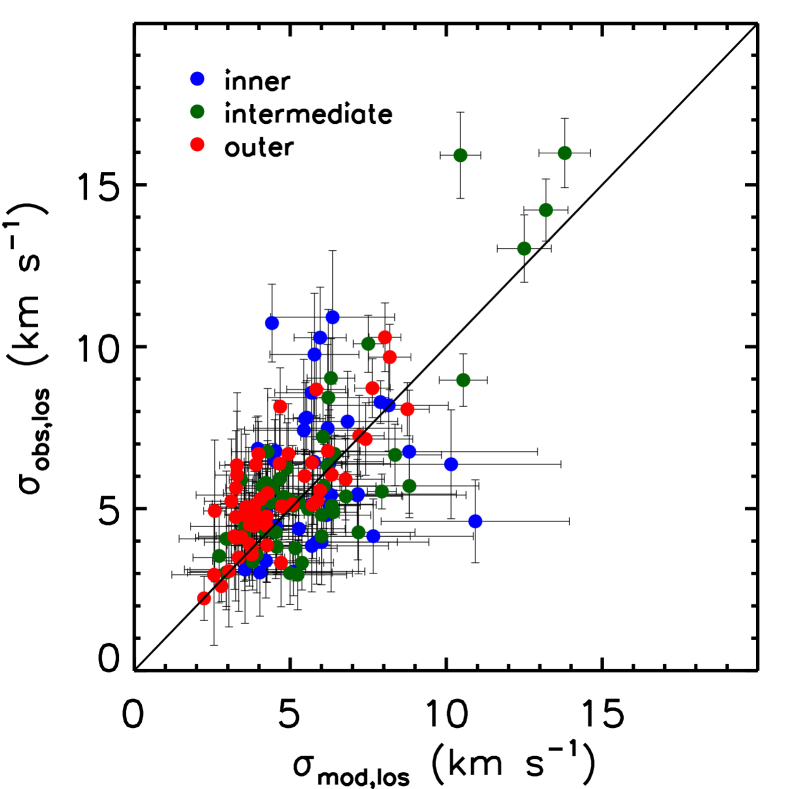
Lastly, if all fluid elements of a cloud follow pure epicyclic motions described by the trigonometric terms in Eqs. 44, the cloud is necessarily in Virial equilibrium (Meidt et al., 2018) and thus the contribution of external gravity should vanish, i.e. and . However, (or equivalently ) measured from our observations of spatially-resolved clouds are clearly not zero (see Section 5.5), suggesting that the bulk motions within the NGC4429 clouds can not be dominated by gravitational epicyclic motions. In turn, we expect the measured (and ) to more closely match those predicted from gravitational shear motions only. As our shear model assumes that all fluid elements of a cloud move on perfectly circular orbits determined by the galactic potential, this model yields (cf. Eqs. 38)
| (48) |
where we have again assumed vertical equilibrium, isotropy in the equatorial plane and . The detailed derivations of these equations and their more general forms for a homogeneous ellipsoidal cloud are provided in Appendix B.
Unsurprisingly, in the shear model the overall effect of external gravity primarily depends on the shear arising from the differential rotation of the galaxy disc (i.e. Oort’s constant ). We note that can be understood as the rotational kinetic energy of a cloud with angular velocity , as generally the rotational kinetic energy and for a spherical cloud. Our derived is the same as that derived by Goldreich & Lynden-Bell (1965) and Fleck & Clark (1981), and it arises naturally when considering fluid element motions near the tidal radius (see Section 6.3). For a galaxy with a solid-body circular velocity curve, the external gravity has no effect on the cloud, i.e. and thus . The distributions of and for axisymmetric and ellipsoidal clouds are shown in the third and fourth panels of Fig 14, respectively, for the spatially-resolved clouds of NGC4429. For clouds assumed to be axisymmetric, a log-normal fit to the distribution of yields a mean and a standard deviation of dex, while a Gaussian fit to the distribution of yields a mean and a standard deviation of . For clouds assumed to be ellipsoidal, analogous fits yield and a standard deviation of dex, and and a standard deviation of . Both sets of predictions therefore compare very well with our measurements ( and for axisymmetric clouds and and for ellipsoidal clouds; see Sections 5.6 and 5.7, respectively), although with less scatter as expected (our model predictions do not take into account measurement errors). This thus supports yet again our conclusion that the bulk motions of the clouds in NGC4429 are primally driven by shear motions. Indeed, our shear model provides good estimates of , and for the spatially-resolved clouds of NGC4429.
It is nevertheless worth noting that, while our shear model accounts for the observed bulk motions of the clouds well, there are also some discrepancies. Our shear model overestimate the angular velocities of the spatially-resolved clouds of NGC4429 by a median factor of , and the modelled and observed position angles have a median angle difference of (see Section 4.2). Moreover, there is considerable scatter about the correlation between the observed velocity dispersions and the modelled velocity dispersions (Fig. 16). It therefore appears that, although the effects of external gravity are dominant, other factors also noticeably affect the dynamics of clouds, so that the clouds’s fluid elements do not follow pure shear motions. We discuss one such factor, self gravity, below.
6.2 Equilibrium between self-gravity and external-gravity
In previous sections, we established that the contributions of external gravity to the gravitational energy budgets of the NGC4429 clouds (i.e. ) are clearly non-zero, this whether these contributions are calculated from observations (Section 5.5) or our shear model (Section 6.1). However, on its own does not determine whether a cloud is gravitationally bound or not. As a robust threshold between gravitationally bound and unbound objects, we have adopted a critical virial parameter (Kauffmann et al., 2013; Kauffmann et al., 2017). When the effective virial parameter is equal to this critical value, (), where
| (49) |
is the kinetic energy of the turbulent motions associated with self-gravity (see Eqs. 34, 32 and 31). If a cloud is thus marginally gravitationally bound (i.e. ) and an internal Virial equilibrium is established by self-gravity (i.e. ), as is the case for the NGC4429 clouds, we further obtain
| (50) |
The top equation indicates an equilibrium between a cloud’s self-gravitational energy and its turbulent kinetic energy, while the bottom equation indicates an equilibrium between a cloud’s self-gravitational energy and its energy contributed by external gravity.
In general, one needs to compare with the self-gravitational energy of a cloud to assess its boundedness. If (i.e. ), then external gravity is much more important and the cloud is not gravitationally bound (unless other forces are present). If (i.e. ), then self-gravity is much more important and the effects of external gravity are negligible. If (i.e. ), then external gravity and self-gravity are equally important and the cloud reaches a state of equilibrium between self-gravity and external gravity. Here, we have found that the NGC4429 clouds have comparable to (the absolute values of) their self-gravitational energies, with both (see Section 5.5) and (see Section 6.1). The energy of each cloud contributed by external gravity thus roughly equals its self-gravitational energy and the cloud remains marginally gravitationally bound.
Tidal radius. In the case where the gravitational motions of the clouds are completely dominated by shear motions, as is the case for the NGC4429 clouds (see Section 6.1), the bottom equation of Eqs. 50 then indicates an equilibrium between a cloud’s self-gravitational energy and its kinetic energy associated with those shear motions. Another way to assess wether self-gravity or external gravity is more important is thus to consider the tidal radius of each cloud, that defines the volume over which self-gravity dominates over external gravity. Here, we adopt the tidal radius defined by Gammie et al. (1991) and Tan (2000), that is the radial distance from the cloud’s center at which the shear velocity due to differential galactic rotation (i.e. our previously-defined ; see Eq. 46) is equal to the escape velocity from the cloud:
| (51) |
where as before is the cloud’s mass and the galactocentric distance of the cloud’s CoM in the plane of the disc, is the total galactic mass interior to , , and as before is the galaxy circular velocity curve. Equation 51 assumes a spherical galaxy mass distribution, i.e. , and can therefore be simplified to
| (52) |
The tidal radius defined in this manner is the maximum size of a cloud (of a given mass ) allowed by galactic rotational shear.
Interestingly, for a cloud with , we have
| (53) |
(see Eqs. 48 and 32), that is essentially identical to the measured of the spatially-resolved clouds of NGC4429 (assuming axisymmetric clouds; see Sections 5.6 and 5.7). In our shear model, the tidal radius given by Eq. 52 thus approximately corresponds to the radial distance at which . It is thus clear the reason a cloud with becomes gravitationally unbound is because the shear motions are so strong that the (outer) fluid elements manage to escape from the self-gravitational influence of the cloud. Figure 17 compares the observed sizes (radii ) of the spatially-resolved clouds of NGC4429 with their tidal radii expected from Eq. 52. There is generally a very good agreement, albeit with a few exceptions. The NGC4429 clouds therefore seem to reach their maximum sizes allowed by galactic shear, further supporting our conclusion that the NGC4429 clouds have reached a rough equilibrium between self-gravity and external gravity and thereby manage to remain marginally gravitationally bound. A few clouds in the inner region have sizes much larger than their tidal radii, suggesting that these inner clouds can not be gravitationally bound due to shear, and indeed all these clouds have high ( – ) and ( – ).
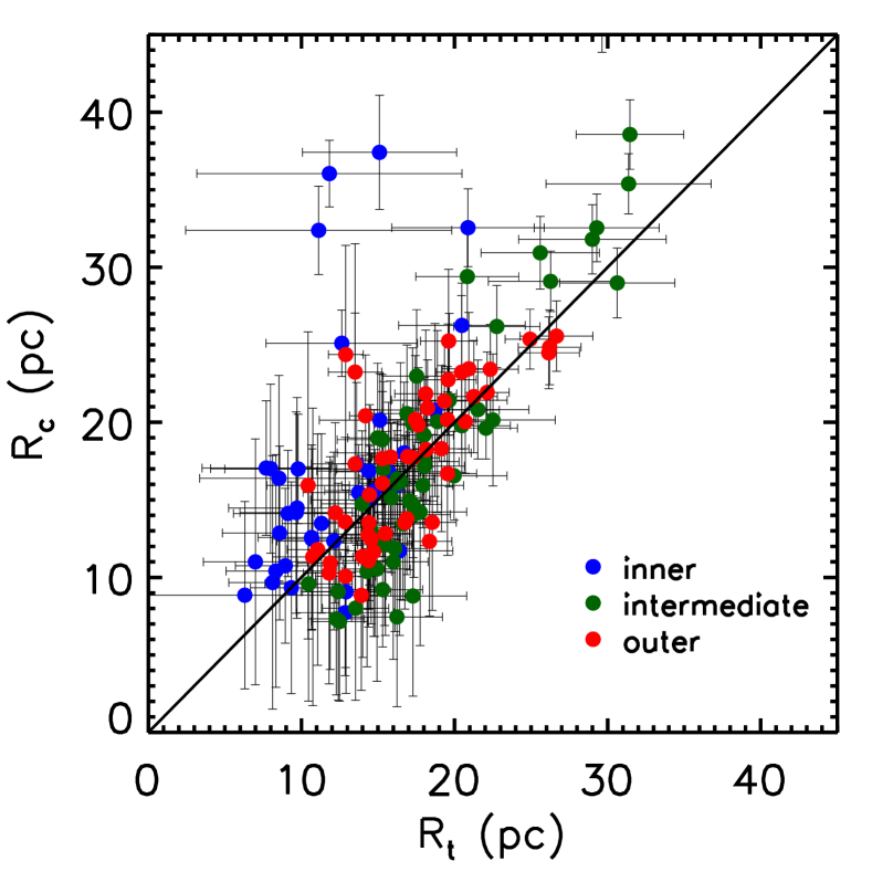
Size and surface density. For a cloud to be marginally gravitationally bound, the contribution of external gravity to the cloud’s energy budget must not exceed the cloud’s self-gravitational energy, i.e. (see Eqs. 48 and 32). This implies that, at a given surface density, there is a maximum size () for a cloud to stay marginally bound against tidal/shear disruptions:
| (54) |
Equivalently, at a given size, there is a minimum surface density () for a cloud to remain marginally bound:
| (55) |
The spatially-resolved clouds of NGC4429 have a mean surface density pc-2 and a mean Oort’s constant (i.e. shear) km s-1 pc-1. A simple calculation using Eq. 54 (and assuming for spherical homogeneous clouds as usual) then suggests that, if limited by shear, the mean size of the clouds in NGC4429 should be pc, that matches extremely well the observed mean size pc. We thus find again that typical clouds in NGC4429 reach their maximal sizes (or minimum surface densities) allowed by shear, and are thus not limited by other processes (shear rules!).
Finally, as we have pointed out above, the effects of self-gravity are generally of the same order as those of external (i.e. galactic) gravity: (see Section 5.6) and . The motions of the fluid elements within these marginally gravitationally-bound clouds will therefore not completely follow those prescribed by external gravity alone (i.e. the shear motions governed by Eqs. 45). This is again expected, as if the bulk motions of cloud fluid elements were to exactly follow pure shear motions, the clouds could not be (marginally) gravitationally bound.
Therefore, the equations of (bulk) motions must include additional terms due to self-gravity (cf. Eqs. 43):
| (56) |
where is the cloud’s own (self) gravitational potential. Solving these coupled differential equations is very difficult and beyond the scope of this paper, although we do derive approximate analytic solutions in Section 6.3 for a particular case. We refer readers to Julian & Toomre (1966), Gammie et al. (1991) and Binney (2020) for some numerical solutions.
Gammie et al. (1991) suggested that Eqs. 45 can provide good-zeroth order solutions to Eqs. 56 at large radii (where ). Therefore, the bulk motions of gravitationally-unbound () clouds should roughly approximate the gravitational shear motions described by Eqs. 45. However, unlike gravitationally-unbound clouds, where the discrepancies between bulk motions and shear motions are expected to be negligible, marginally gravitationally-bound clouds should have bulk motions that deviate considerably from shear motions. This is because the discrepancies between bulk motions and shear motions should increase with the importance of self-gravity. Indeed, while the bulk motions of the NGC4429 clouds do approximately follow gravitational shear motions, noticeable deviations are also found (see Section 6.1). We provide approximate solutions for this case below.
6.3 Cloud morphology
Cloud morphology may reflect the origin of the gas motions (e.g. Meidt et al., 2018) and the physical mechanisms injecting energy into the gas on cloud scales (e.g. Koda et al., 2006). To quantify the morphology of the spatially-resolved clouds of NGC4429, we considered their major and minor axes (and thus their axis ratios and position angles with respect to the radial/galactocentric direction) as measured in the plane of the sky (i.e. deprojected) in Section 5.7.
The distribution of the deprojected clouds’ axis ratios is shown in the left panel of Fig. 18. A Gaussian fit to the distribution yields a mean of , suggesting that the clouds of NGC4429 are significantly elongated. Moreover, the clouds in the inner and intermediate regions are more elongated (mean axis ratio of and , respectively) than the clouds in the outer region (mean axis ratio of ).
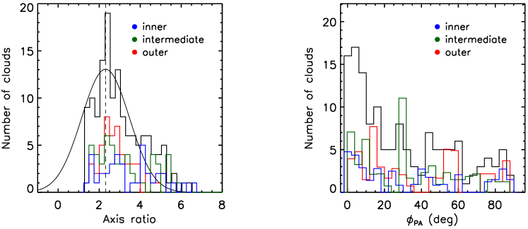
The distribution of deprojected position angles is shown in the right panel of Fig. 18. The distribution peaks at , with a mean , confirming the impression from Fig. 3 that the clouds of NGC4429 are preferentially elongated in the radial (i.e. galactocentric) direction. In fact, the clouds at small radii tend to have smaller , i.e. they are even more preferentially elongated in the direction of the galaxy centre. The mean angle of the clouds in the inner, intermediate and outer region is , and , respectively.
It is worth noting that the tendency for the clouds to align with the radial direction could at least partially be due to an artefact of CPROPS. As CPROPS tends to assign the pixels with the shortest “distances” (through the 3D data cube) to the same cloud, the clouds identified by CPROPS could be preferentially elongated along the isovelocity contours, that are often nearly radial in NGC4429 (see Fig. 7). Having said that, we note that the clouds identified by CPROPS in other galaxies do not seem to exhibit such a tendency (e.g. NGC4526, Utomo et al. 2015; M33, Gratier et al. 2012; NGC6946, Wu et al. 2017). This thus suggests that the observed trend of the clouds of NGC4429 to be radially elongated could be real.
If the observed tendency is real, what are the physical mechanisms that could cause such a strong radial elongation of the clouds of NGC4429? It is interesting to note that, according to Eq. 53,
| (57) |
which suggests that if then (and vice-versa) and if then (and vice-versa). If a cloud is primarily dominated by self-gravity (i.e. or ), the effects of external gravity are negligible and the cloud should be roughly round. On the other hand, if a cloud is largely dominated by external gravity (i.e. or ), the cloud should be elongated in the azimuthal direction due to strong shear motions (Meidt et al., 2018). However, the NGC4429 clouds are neither round nor azimuthally elongated, suggesting their morphologies can not be regulated by either self-gravity and/or external gravity alone.
It is thus interesting to investigate the geometry of a marginally gravitationally-bound cloud, as is the case for the bulk of the NGC4429 clouds, where both self-gravity and external gravity are important (i.e. and ; see Sections 5.6 and 6.2). For this, we must solve the equations of motions given by Eqs. 56, that include both self-gravity and external gravity terms. If we can calculate the motions of the fluid elements near the external edge of each cloud, these motions will define the approximate overall shapes of marginally gravitationally-bound clouds.
Exact analytic solutions to Eqs. 56 may not be possible, so we instead turn to a mathematical technique analogous to perturbation theory to find approximate solutions. We define a new dimensionless variable and rewrite Eqs. 56 as
| (58) |
Approximate solutions to the above equations can be written as
| (59) |
where analogously to perturbation theory we will refer to and as the zeroth-order solutions and to and as the first-order solutions, although the latter are not necessarily smaller than the former. Substituting Eqs. 59 into Eqs. 58, we can separate the zeroth- and first-order equations in :
| (60) |
and
| (61) |
We note that the solutions to Eqs. 60 – 61 provide solutions to Eqs. 58 for only a particular case, and they are only approximate solutions as the second-order term in is assumed to be negligible, i.e. (assumptions we will justify below).
We first solve the zeroth-order equations. While finding a general analytic solution to the Eqs. 60 is beyond the scope of this paper, there must exist a particular cloudcentric radius where to zeroth order the fluid element has uniform circular motion of a particular angular frequency (and arbitrary phase ). We thus postulate
| (62) |
Substituting Eqs. 62 into the first equation of Eqs. 60, we find that the first and second terms on the RHS (i.e. the tidal and Coriolis force terms) cancel out only for an angular frequency (as ). While shear does not lead to circular motions, that is of course simply equal to (see Eq. 46), i.e.
| (63) |
(the same defined in Section 6.1). The term on the left-hand side and the third term on the RHS then lead to a condition on . Assuming the entire cloud mass is contained within , one obtains
| (64) |
(see Eq. 52). The same condition is obtained by substituting Eqs. 62 into the second equation of Eqs. 60. It is trivial to show that at this radius, , where is the circular velocity due to the cloud alone (i.e. for given by Eq. 64).
In other words, the (zeroth-order in ) solution to Eqs. 60 is
| (65) |
where is given by Eq. 64. This orbit is thus intuitive to understand. In the cloud rotating frame, to zeroth order, the fluid element will have uniform circular motion at the radius where the shear velocity due to the external (i.e. galactic) potential is equal to the cloud’s own circular velocity , and thus the shear angular velocity is equal to the cloud’s angular velocity (i.e. ).
Equally important, the radius of this circular orbit is very close to the tidal radius and thus the external edge of the cloud ( according to Eq. 64). Our solutions can thus indeed help us understand the outer shapes of marginally-bound clouds.
We note that our zeroth-order solutions in above are different from those found in Goldreich & Tremaine (1982) and Gammie et al. (1991) (Eqs. 45 in this paper). This is because we introduced in the azimuthal Coriolis force term while they applied to the self-gravity terms, and because we are considering a particular case where the fluid element’s shear velocity is equal to its circular velocity. Equations 65 thus suggest that the fluid element should have a circular orbit about the cloud’s CoM (i.e. the cloud should be round near its tidal radius) if the Coriolis force in the azimuthal direction is neglected (the term in the second equation of Eqs. 56). This is not surprising, since as we have shown the Coriolis force () cancels out the tidal force () in the radial direction, hence only the cloud’s self-gravity needs to be considered.
Having solved the zeroth-order equations of motion (Eqs. 60), we can now solve the first-order equations in (Eqs. 61). Substituting the first equation of Eqs. 65 into the second equation of Eqs. 61 and imposing that the fluid element follows the zeroth-order solution at (i.e. ) yields a solution for . Substituting this in turn into the first equation of Eqs. 61 and imposing again that the fluid element follows the zeroth-order solution at (i.e. ) yields a solution for . These first-order solution are
| (66) |
We therefore have complete zeroth- and first-order solutions in of the equations of motion Eqs. 58, for fluid elements originally in uniform circular rotation around the cloud’s CoM at a cloudcentric radius of .
In practice, with our treatment in term of , we have neglected the firt-order Coriolis force term in the azimuthal direction (i.e. the term in the second equation of Eqs. 56). Our solutions will thus only be valid as long as this term remains small compared to . A comparison of these two terms shows that this remains the case for times up to several for nearly all phases , when the fluid element remains relatively close to the circle of radius .
By sampling the phases uniformly, Figure 19 therefore shows how a circular ring of matter initially at a cloudcentric radius evolves over time (colour-coded), up to a time . As expected from our solutions, particularly the diverging term in (see Eqs. 66), the fluid element orbits and thus the ring become increasingly elongated over time, this almost always in the radial direction (i.e. along ), more so but not exclusively at late times.
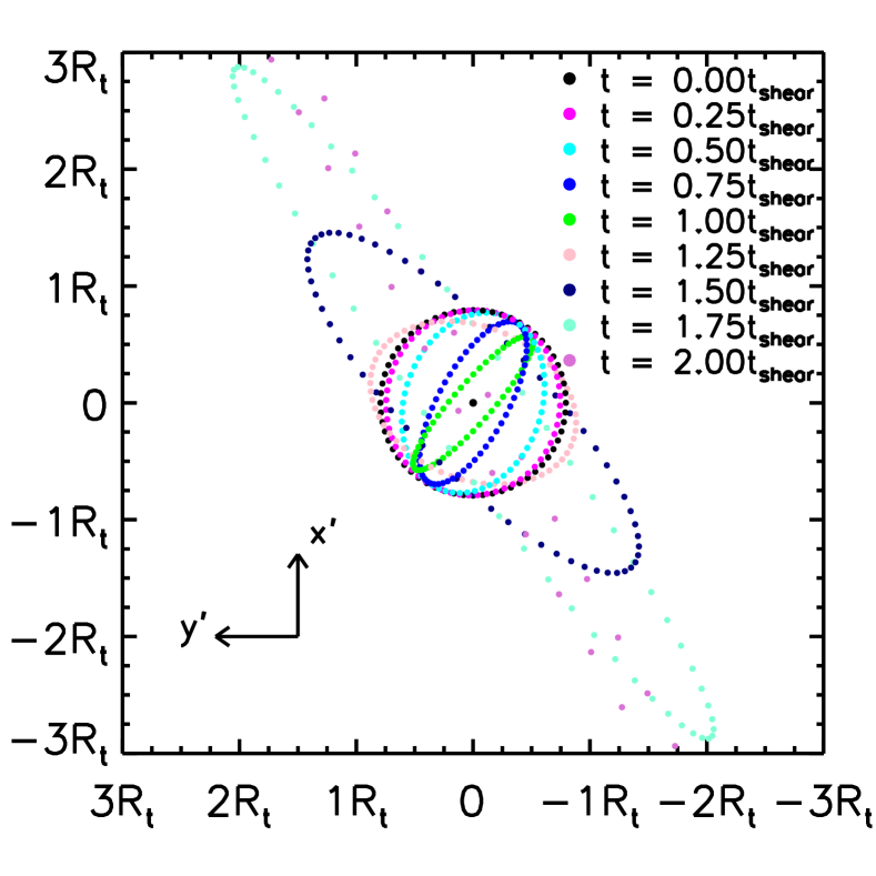
Therefore, contrary to naive expectations, clouds with sizes and thus , that are necessarily marginally-bound, should have shapes that are radially elongated. This state thus presumably represents an intermediate state between i) small strongly-bound clouds that are expected to be spherical (due to self-gravity) and ii) large unbound gas accumulations that are expected to be azimuthally elongated (due to shear). In other words, the general radial elongation of the NGC4429 clouds is fully consistent with the fact that the clouds extend to typically their tidal radii and are typically marginally gravitationally bound, with roughly equal impact from self- and external gravity (i.e. ).
Interestingly, the numerical solutions of Julian & Toomre (1966) and Binney (2020) suggest a similar result. By solving Eqs. 56 numerically, they derived density patterns for a shear flow under both self- and external gravity forces. While the outer contours at lower surface densities (where self-gravity is much less important than external gravity) are elongated azimuthally as expected, their results demonstrate that the innermost contours at higher densities (where self-gravity may be as important as external gravity) are radially elongated (see Figs. – in Julian & Toomre 1966 and Fig. in Binney 2020). These works thus reinforce our approximate analytical solutions above.
6.4 Cloud scale height
Our current analysis is based on the common assumption that the clouds of NGC4429 are in vertical hydrostatic equilibria, i.e. (see Eq. 27). If this assumption is valid, we can derive the scale height of each cloud () from estimates of and . As before, is obtained directly from our stellar mass model (i.e. , where is provided by our our MGE model; see Appendix C). According to Eq. 20, , so if can indeed be derived from Eq. 24 (i.e. ), we can obtain .
We note that the uncertainties of our measured physical quantities (i.e. , and ) can be significant and prevent us from accurately estimating for individual clouds, as we find negative in a few cases. Instead, we therefore consider only the average quantities for and . We derive a mean km2 s-2 for the spatially-resolved clouds of NGC4429 (assuming for spherical homogeneous clouds), whose mean line-of-sight projection ( km2 s-2) is indeed relatively small compared to km2 s-2 and km2 s-2.
Utilising our derived km2 s-2 and pc-3 (and further assuming for spherical homogeneous clouds), we derive a mean cloud scale height pc, that is clearly smaller than the average cloud radius pc (see Section 3.3). Consequently, the clouds of NGC4429 are not strictly spherical, but more likely to be elongated (i.e. flattened) in the plane, if the clouds are indeed in vertical hydrostatic equilibria.
The above analysis aimed to derive the scale heights of the clouds by assuming that the clouds are in vertical hydrostatic equilibria. However, we can also investigate the vertical equilibrium state of the clouds by assuming instead. For such a roundish cloud, the contribution of the vertical component of the external potential to the cloud’s gravitational energy budget is . We thus define as the ratio between and the (absolute value of the) self-gravitational energy of a roundish cloud ():
| (67) |
The distribution of for the spatially-resolved clouds of NGC4429 is presented in Fig. 20, where we have assumed (spherical homogeneous clouds) as usual. We find that is not negligible, but significantly below zero. A Gaussian fit to the distribution yields a mean . This implies that the effect of external gravity on roundish clouds is to compress them in the vertical direction. In other words, if the clouds of NGC4429 were roundish, the shear in the plane of the galaxy would be overwhelmed by compression in the vertical direction, and the net effect of external gravity would be to contribute to the (vertical) collapse of the clouds (as ). This probably explains why the clouds of NGC4429 appear to be flattened in the plane.
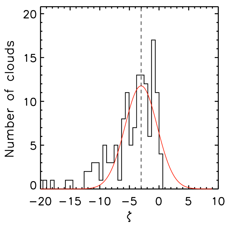
Indeed, a cloud in a thin disc is more likely to exhibit an elongated structure in the plane rather than be spherical, as the force applied by the background galactic potential in the vertical direction far exceeds the forcing experienced in the plane (e.g. Meidt et al., 2018). In fact, such elongations of molecular clouds in the equatorial plane have been observed in a sample of more than MW clouds (Koda et al., 2006).
7 Conclusions
Using our modified version of the CPROPSTOO code, more robust and efficient to identify GMCs in complex and crowded environments, and 12CO ALMA observations at pc2 resolution, we identified GMCs ( spatially resolved) in the central molecular gas disc of the lenticular galaxy NGC4429. To investigate the dynamical states of the GMCs, we developed and utilised a modified Virial theorem that fully accounts for the impacts of the background galactic potential. The main results are as follows:
-
1.
The GMCs of NGC4429 appear to have smaller sizes ( – pc), lower gaseous masses ( – ), higher gaseous mass surface densities ( – pc-2) and higher observed linewidths ( – km s-1) than the GMCs of the Milky Way disc and other Local Group galaxies.
-
2.
Cloud properties exhibit several trends with galactocentric distance. Specifically, except for the three innermost resolved clouds at pc, the GMCs at small radii tend to have smaller sizes, lower gaseous masses, higher gaseous mass surface densities and higher observed linewidths than clouds farther out. However, we also find that all these quantities drop abruptly in the outermost region of the molecular gas disc ( pc).
-
3.
The GMCs of NGC4429 appear to be elongated (mean axis ratio of ) and are preferentially aligned in the radial direction (i.e. toward the galactic centre). The clouds also appear to be flattened in the plane of the galaxy.
-
4.
The cloud mass distribution follows a truncated power law with slope and truncation mass , suggesting most of the molecular mass of NGC4429 is in low-mass clouds. We find a slight variation of the mass spectrum with galactocentric distance, suggesting massive clouds are more favoured at intermediate radii ( pc).
-
5.
Strong velocity gradients are observed within individual GMCs ( – km s-1 pc-1), significantly larger than those of GMCs in the MW and other Local Group galaxies. A steep size – line width relation (with a power-law index ) and large observed Virial parameters () are also found for the clouds of NGC4429. However, we argue the large velocity gradients, steep size – line width relation and large observed Virial parameters are all a consequence of gas motions driven by the background galactic potential (i.e. local circular orbital rotation), not the clouds’ self-gravity. To remove the contribution of galaxy rotation from the clouds’ linewidths and derive linewidths quantifying turbulence only, we measure the gradient-subtracted linewidths of the clouds . Using this measure, an internal Virial equilibrium appears to have been reached betweem the clouds’ turbulent kinetic energies () and their self-gravitational energies (), i.e. .
-
6.
However, we argue that neither nor reflects the true dynamical state of a cloud. We thus discuss and revisit the conventional Virial theorem, deriving a modified theorem that explicitly takes into account both the self-gravity of the clouds and the effects of the external (galactic) gravitational potential in the vertical direction and the plane separately. This allows us to define an effective velocity dispersion and an effective Virial parameter , that provide straightforward measurable diagnostics of cloud boundedness in the presence of a non-negligeable external potential.
-
7.
Using our new diagnostics, we find the contributions of external gravity to the clouds’ energy budgets are generally much larger than zero. This is because the bulk motions of the clouds are dominated by gravitational shear motions rather than epicyclic motions. The clouds of NGC4429 are in a critical state in which the energy contributed by external gravity is approximately equal to the self-gravitational energy, i.e. . As such, the clouds are not virialised but remain marginally gravitationally bound, with a mean effective Virial parameter ( and ) close to the threshold between gravitationally-bound and unbound objects (). This is also true when the elongated shapes of the clouds are taken into account ( and for ellipsoidal clouds). As the clouds appear to reach an equilibrium between self-gravity and external gravity, they also have sizes consistent with their tidal radii (i.e. ) and are radially elongated (with an average axis ratio of ). Overall, external gravity appears to be as important as self-gravity to regulate the morphologies, dynamics and thus ultimately the fates of the clouds.
-
8.
Galactic rotational shear appears to play a dominant role to regulate the properties of the clouds of NGC4429. Our shear model predicts that, as rotational shear increases, the contribution of external gravity to a cloud’s energy budget also increases and the cloud becomes less bound, leading to a maximum size (or equivalently a minimum gaseous mass surface density) for the cloud to remain marginally bound: (), that matches very well the observed sizes of the clouds of NGC4429.
Acknowledgements
We thank Michele Cappellari, Marc Sarzi, Christopher McKee and James Binney for valuable discussions. MB was supported by STFC consolidated grant ’Astrophysics at Oxford" ST/H002456/1 and ST/K00106X/1. MC acknowledges support from a Royal Society University Research Fellowship. TAD acknowledges support from a STFC Ernest Rutherford Fellowship. MDS acknowledges support from a STFC DPhil studentship ST/N504233/1. KO was supported by Shimadzu Science and Technology Foundation. This publication arises from research funded by the John Fell Oxford University Press Research Fund.
This paper makes use of the following ALMA data: ADS/JAO.ALMA#2013.1.00493.S. ALMA is a partnership of ESO (representing its member states), NSF (USA) and NINS (Japan), together with NRC (Canada) and NSC and ASIAA (Taiwan) and KASI (Republic of Korea), in cooperation with the Republic of Chile. The Joint ALMA Observatory is operated by ESO, AUI/NRAO and NAOJ. This paper also makes use of observations made with the NASA/ESA Hubble Space Telescope, and obtained from the Hubble Legacy Archive, which is a collaboration between the Space Telescope Science Institute (STScI/NASA), the Space Telescope European Coordinating Facility (ST-ECF/ESA) and the Canadian Astronomy Data Centre (CADC/NRC/CSA). This research has made use of the NASA/IPAC Extragalactic Database (NED) which is operated by the Jet Propulsion Laboratory, California Institute of Technology, under contract with the National Aeronautics and Space Administration.
DATA AVALABILITY
The data underlying this article is available in the ALMA archive (https://almascience.eso.org/asax/) under project code 2013.1.00493.S.
References
- Adelman-McCarthy et al. (2008) Adelman-McCarthy J. K., et al., 2008, ApJS, 175, 297
- Alatalo et al. (2013) Alatalo K., et al., 2013, MNRAS, 432, 1796
- Ballesteros-Paredes (2006) Ballesteros-Paredes J., 2006, MNRAS, 372, 443
- Ballesteros-Paredes et al. (2006) Ballesteros-Paredes J., Gazol A., Kim J., Klessen R. S., Jappsen A.-K., Tejero E., 2006, ApJ, 637, 384
- Ballesteros-Paredes et al. (2007) Ballesteros-Paredes J., Klessen R. S., Mac Low M.-M., Vazquez-Semadeni E., 2007, Protostars and Planets V, pp 63–80
- Ballesteros-Paredes et al. (2009) Ballesteros-Paredes J., Gómez G. C., Pichardo B., Vázquez-Semadeni E., 2009, MNRAS, 393, 1563
- Ballesteros-Paredes et al. (2011) Ballesteros-Paredes J., Hartmann L. W., Vázquez-Semadeni E., Heitsch F., Zamora-Avilés M. A., 2011, MNRAS, 411, 65
- Bertoldi & McKee (1992) Bertoldi F., McKee C. F., 1992, ApJ, 395, 140
- Binney (2020) Binney J., 2020, MNRAS, 496, 767
- Binney & Tremaine (2008) Binney J., Tremaine S., 2008, Galactic Dynamics: Second Edition. Princeton University Press
- Blitz (1993) Blitz L., 1993, in Levy E. H., Lunine J. I., eds, Protostars and Planets III. pp 125–161
- Blitz et al. (2007) Blitz L., Fukui Y., Kawamura A., Leroy A., Mizuno N., Rosolowsky E., 2007, Protostars and Planets V, pp 81–96
- Bolatto et al. (2008) Bolatto A. D., Leroy A. K., Rosolowsky E., Walter F., Blitz L., 2008, ApJ, 686, 948
- Bolatto et al. (2013) Bolatto A. D., Wolfire M., Leroy A. K., 2013, ARA&A, 51, 207
- Burkert & Bodenheimer (2000) Burkert A., Bodenheimer P., 2000, ApJ, 543, 822
- Camacho et al. (2016) Camacho V., Vázquez-Semadeni E., Ballesteros-Paredes J., Gómez G. C., Fall S. M., Mata-Chávez M. D., 2016, ApJ, 833, 113
- Cappellari (2002) Cappellari M., 2002, MNRAS, 333, 400
- Cappellari (2008) Cappellari M., 2008, MNRAS, 390, 71
- Cappellari et al. (2011) Cappellari M., et al., 2011, MNRAS, 416, 1680
- Cappellari et al. (2013) Cappellari M., et al., 2013, MNRAS, 432, 1862
- Chen et al. (2016) Chen X., Amaro-Seoane P., Cuadra J., 2016, ApJ, 819, 138
- Colombo et al. (2014) Colombo D., et al., 2014, ApJ, 784, 3
- Colombo et al. (2018) Colombo D., et al., 2018, Monthly Notices of the Royal Astronomical Society, 483, 4291
- Dale et al. (2019) Dale J. E., Kruijssen J. M. D., Longmore S. N., 2019, MNRAS, 486, 3307
- Dame et al. (2001) Dame T. M., Hartmann D., Thaddeus P., 2001, ApJ, 547, 792
- Davis (2014) Davis T. A., 2014, MNRAS, 445, 2378
- Davis et al. (2011) Davis T. A., et al., 2011, MNRAS, 417, 882
- Davis et al. (2013) Davis T. A., et al., 2013, MNRAS, 429, 534
- Davis et al. (2017) Davis T. A., Bureau M., Onishi K., Cappellari M., Iguchi S., Sarzi M., 2017, MNRAS, 468, 4675
- Davis et al. (2018) Davis T. A., et al., 2018, MNRAS, 473, 3818
- Dib et al. (2012) Dib S., Helou G., Moore T. J. T., Urquhart J. S., Dariush A., 2012, ApJ, 758, 125
- Donovan Meyer et al. (2012) Donovan Meyer J., et al., 2012, ApJ, 744, 42
- Donovan Meyer et al. (2013) Donovan Meyer J., et al., 2013, ApJ, 772, 107
- Elmegreen (1989) Elmegreen B. G., 1989, ApJ, 338, 178
- Elmegreen & Falgarone (1996) Elmegreen B. G., Falgarone E., 1996, ApJ, 471, 816
- Emsellem et al. (1994) Emsellem E., Monnet G., Bacon R., 1994, A&A, 285, 723
- Emsellem et al. (2011) Emsellem E., et al., 2011, MNRAS, 414, 888
- Engargiola et al. (2003) Engargiola G., Plambeck R. L., Rosolowsky E., Blitz L., 2003, ApJS, 149, 343
- Faesi et al. (2016) Faesi C. M., Lada C. J., Forbrich J., 2016, ApJ, 821, 125
- Faesi et al. (2018) Faesi C. M., Lada C. J., Forbrich J., 2018, ApJ, 857, 19
- Falgarone et al. (1991) Falgarone E., Phillips T. G., Walker C. K., 1991, ApJ, 378, 186
- Field et al. (2008) Field G. B., Blackman E. G., Keto E. R., 2008, MNRAS, 385, 181
- Field et al. (2011) Field G. B., Blackman E. G., Keto E. R., 2011, MNRAS, 416, 710
- Fleck (1980) Fleck Jr. R. C., 1980, ApJ, 242, 1019
- Fleck & Clark (1981) Fleck Jr. R. C., Clark F. O., 1981, ApJ, 245, 898
- Fukui et al. (2008) Fukui Y., et al., 2008, ApJS, 178, 56
- Gammie et al. (1991) Gammie C. F., Ostriker J. P., Jog C. J., 1991, ApJ, 378, 565
- Goldreich & Lynden-Bell (1965) Goldreich P., Lynden-Bell D., 1965, MNRAS, 130, 125
- Goldreich & Tremaine (1982) Goldreich P., Tremaine S., 1982, ARA&A, 20, 249
- Gratier et al. (2012) Gratier P., et al., 2012, A&A, 542, A108
- Hennebelle & Chabrier (2013) Hennebelle P., Chabrier G., 2013, ApJ, 770, 150
- Henshaw et al. (2019) Henshaw J. D., et al., 2019, MNRAS, 485, 2457
- Heyer et al. (2009) Heyer M., Krawczyk C., Duval J., Jackson J. M., 2009, ApJ, 699, 1092
- Hirota et al. (2011) Hirota A., Kuno N., Sato N., Nakanishi H., Tosaki T., Sorai K., 2011, ApJ, 737, 40
- Hughes et al. (2010) Hughes A., et al., 2010, MNRAS, 406, 2065
- Hughes et al. (2013) Hughes A., et al., 2013, ApJ, 779, 46
- Ibáñez-Mejía et al. (2016) Ibáñez-Mejía J. C., Mac Low M.-M., Klessen R. S., Baczynski C., 2016, ApJ, 824, 41
- Imara & Blitz (2011) Imara N., Blitz L., 2011, ApJ, 732, 78
- Imara & Faesi (2019) Imara N., Faesi C. M., 2019, ApJ, 876, 141
- Imara et al. (2011) Imara N., Bigiel F., Blitz L., 2011, ApJ, 732, 79
- Julian & Toomre (1966) Julian W. H., Toomre A., 1966, ApJ, 146, 810
- Kauffmann et al. (2013) Kauffmann J., Pillai T., Zhang Q., 2013, ApJ, 765, L35
- Kauffmann et al. (2017) Kauffmann J., Pillai T., Zhang Q., Menten K. M., Goldsmith P. F., Lu X., Guzmán A. E., 2017, A&A, 603, A89
- Koda et al. (2006) Koda J., Sawada T., Hasegawa T., Scoville N. Z., 2006, ApJ, 638, 191
- Koyama & Ostriker (2009) Koyama H., Ostriker E. C., 2009, ApJ, 693, 1346
- Kruijssen et al. (2019) Kruijssen J. M. D., et al., 2019, MNRAS, 484, 5734
- Larson (1981) Larson R. B., 1981, MNRAS, 194, 809
- Lequeux (2005) Lequeux J., 2005, The Interstellar Medium, doi:10.1007/b137959.
- Leroy et al. (2015) Leroy A. K., et al., 2015, ApJ, 801, 25
- Leroy et al. (2016) Leroy A. K., et al., 2016, ApJ, 831, 16
- Lin et al. (2007) Lin G., Chawla M., Olson K., Barnes C., Guzowsk J., Bjornss C., Shain W., Roysam B., 2007, Cytometry A, 71, 724
- Lombardi et al. (2010) Lombardi M., Alves J., Lada C. J., 2010, A&A, 519, L7
- Mac Low & Klessen (2004) Mac Low M.-M., Klessen R. S., 2004, Reviews of Modern Physics, 76, 125
- MacLaren et al. (1988) MacLaren I., Richardson K. M., Wolfendale A. W., 1988, ApJ, 333, 821
- McKee (1989) McKee C. F., 1989, ApJ, 345, 782
- McKee (1999) McKee C. F., 1999, in Lada C. J., Kylafis N. D., eds, NATO Advanced Study Institute (ASI) Series C Vol. 540, The Origin of Stars and Planetary Systems. p. 29 (arXiv:astro-ph/9901370)
- Meidt (2016) Meidt S. E., 2016, ApJ, 818, 69
- Meidt et al. (2013) Meidt S. E., et al., 2013, ApJ, 779, 45
- Meidt et al. (2015) Meidt S. E., et al., 2015, ApJ, 806, 72
- Meidt et al. (2018) Meidt S. E., et al., 2018, ApJ, 854, 100
- Melchior & Combes (2017) Melchior A.-L., Combes F., 2017, A&A, 607, L7
- Miura et al. (2018) Miura R. E., Espada D., Hirota A., Nakanishi K., Bendo G. J., Sugai H., 2018, ApJ, 864, 120
- Miville-Deschenes et al. (2017a) Miville-Deschenes M. A., Murray N., Lee E. J., 2017a, VizieR Online Data Catalog, p. J/ApJ/834/57
- Miville-Deschênes et al. (2017b) Miville-Deschênes M.-A., Murray N., Lee E. J., 2017b, ApJ, 834, 57
- Muller et al. (2010) Muller E., et al., 2010, ApJ, 712, 1248
- North et al. (2019) North E. V., et al., 2019, MNRAS, 473, 3818
- Nyland et al. (2016) Nyland K., et al., 2016, MNRAS, 458, 2221
- Oka et al. (2001) Oka T., Hasegawa T., Sato F., Tsuboi M., Miyazaki A., Sugimoto M., 2001, ApJ, 562, 348
- Onishi et al. (2017) Onishi K., Iguchi S., Davis T. A., Bureau M., Cappellari M., Sarzi M., Blitz L., 2017, MNRAS, 468, 4663
- Padoan et al. (2017) Padoan P., Haugbølle T., Nordlund Å., Frimann S., 2017, ApJ, 840, 48
- Pan & Kuno (2017) Pan H.-A., Kuno N., 2017, ApJ, 839, 133
- Phillips (1999) Phillips J. P., 1999, A&AS, 134, 241
- Rebolledo et al. (2015) Rebolledo D., Wong T., Xue R., Leroy A., Koda J., Donovan Meyer J., 2015, ApJ, 808, 99
- Rice et al. (2016) Rice T. S., Goodman A. A., Bergin E. A., Beaumont C., Dame T. M., 2016, ApJ, 822, 52
- Rosolowsky (2005) Rosolowsky E., 2005, PASP, 117, 1403
- Rosolowsky (2007) Rosolowsky E., 2007, ApJ, 654, 240
- Rosolowsky & Blitz (2005) Rosolowsky E., Blitz L., 2005, ApJ, 623, 826
- Rosolowsky & Leroy (2006) Rosolowsky E., Leroy A., 2006, PASP, 118, 590
- Rosolowsky et al. (2003) Rosolowsky E., Engargiola G., Plambeck R., Blitz L., 2003, ApJ, 599, 258
- Rosolowsky et al. (2007) Rosolowsky E., Keto E., Matsushita S., Willner S. P., 2007, ApJ, 661, 830
- Rousseeuw & Driessen (2006) Rousseeuw P., Driessen K., 2006, Computing LTS regression for large data sets, 12, 29
- Schruba et al. (2019) Schruba A., Kruijssen J. M. D., Leroy A. K., 2019, ApJ, 883, 2
- Smith et al. (2019) Smith M. D., et al., 2019, MNRAS, 473, 3818
- Smith et al. (2020b) Smith M. D., et al., 2020b, MNRAS, submitted
- Smith et al. (2020a) Smith M. D., et al., 2020a, MNRAS, submitted
- Solomon et al. (1987) Solomon P. M., Rivolo A. R., Barrett J., Yahil A., 1987, ApJ, 319, 730
- Stark & Blitz (1978) Stark A. A., Blitz L., 1978, ApJ, 225, L15
- Strong et al. (1988) Strong A. W., et al., 1988, A&A, 207, 1
- Sun et al. (2018) Sun J., et al., 2018, ApJ, 860, 172
- Tan (2000) Tan J. C., 2000, ApJ, 536, 173
- Tasker & Tan (2009) Tasker E. J., Tan J. C., 2009, ApJ, 700, 358
- Thilliez et al. (2014) Thilliez E., Maddison S. T., Hughes A., Wong T., 2014, Publ. Astron. Soc. Australia, 31, e003
- Tosaki et al. (2017) Tosaki T., et al., 2017, PASJ, 69, 18
- Utomo et al. (2015) Utomo D., Blitz L., Davis T., Rosolowsky E., Bureau M., Cappellari M., Sarzi M., 2015, ApJ, 803, 16
- Utreras et al. (2020) Utreras J., et al., 2020, ApJ, 892, 94
- Verschuur (1993) Verschuur G. L., 1993, AJ, 106, 2580
- Williams et al. (1994) Williams J. P., de Geus E. J., Blitz L., 1994, ApJ, 428, 693
- Wong et al. (2011) Wong T., et al., 2011, ApJS, 197, 16
- Wong et al. (2019) Wong T., et al., 2019, ApJ, 885, 50
- Wu et al. (2017) Wu Y.-L., Sakamoto K., Pan H.-A., 2017, ApJ, 839, 6
- Yang & Ahuja (2014) Yang H., Ahuja N., 2014, Pattern Recognit, 47, 2266
- Young et al. (2011) Young L. M., et al., 2011, MNRAS, 414, 940
- Yusef-Zadeh et al. (2016) Yusef-Zadeh F., Wardle M., Schödel R., Roberts D. A., Cotton W., Bushouse H., Arendt R., Royster M., 2016, ApJ, 819, 60
Appendix A Modified Virial Theorem
Our goal in this appendix is to derive a modified Virial theorem (MVT), that encompasses not only a cloud’s self-gravity, but also the effects of the external (i.e. galactic) potential. We thus envision each cloud as a continuous structure with well-defined borders in position- and velocity-space, located in a rotating gas disc with a circular velocity determined by an axisymmetric background galactic gravitational potential (). We assume each cloud has a homogeneous density distribution and an ellipsoidal geometry. The cloud’s centre of mass (CoM) and its two semi-axes (semi-major axis and semi-minor axis ) are assumed to be located in the orbital plane (i.e. the mid-plane of the galaxy disc; see Fig. 21). We assume each fluid element of a cloud experiences two kinds of motions: (1) random turbulent motions (velocity dispersion ) arising from self-gravity (i.e. the cloud’s own gravitational potential ) and (2) bulk gravitational motions (velocity and root mean square (RMS) velocity ) arising from the external gravity (i.e. the galactic gravitational potential ). We neglect thermal motions, as they are often small compared to turbulent motions in a cold gas cloud (e.g. Fleck, 1980). The turbulent motions due to self-gravity are expected to be quasi-isotropic in three dimensions (Field et al., 2008; Ballesteros-Paredes et al., 2011), while the gas motions induced by the external gravitational potential are often non-isotropic (Meidt et al., 2018). We assume the cloud’s own gravitational potential to be (statistically) independent of the local external gravitational potential , and the motions due to self-gravity () to be uncorrelated with the motions due to external gravitational potential (), as suggested by Meidt et al. (2018). We ignore external pressure and magnetic fields, and consider only the effects of self-gravity and external gravity.
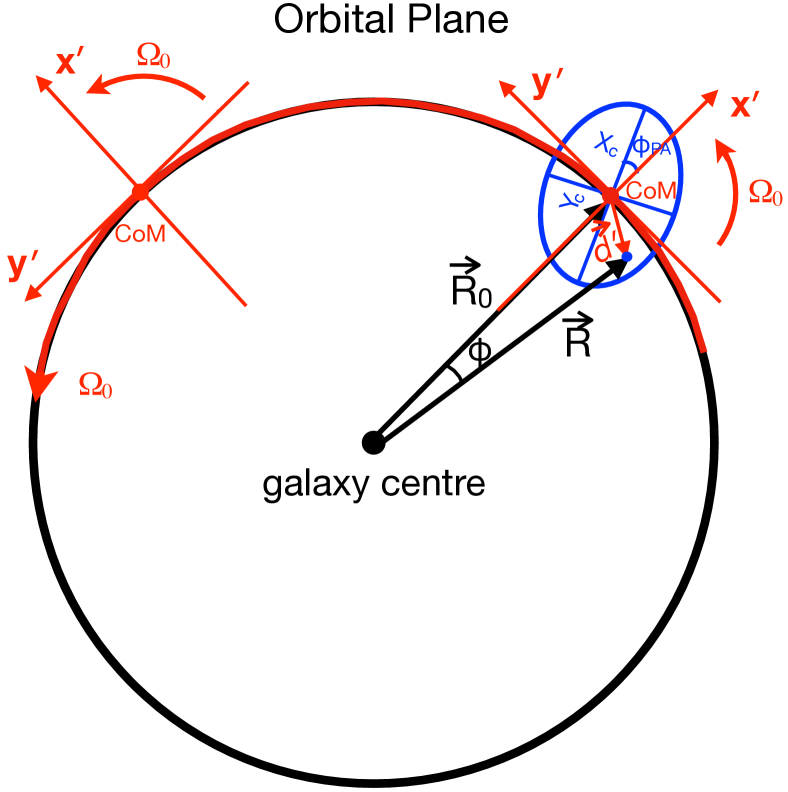
Assuming the surface terms are negligible (Larson, 1981), the general form of the Virial theorem for a cloud is
| (68) |
(see e.g. Eqs. 14.6 and 14.7 of Lequeux 2005), where is the cloud’s moment of inertia, its total kinetic energy, the position vector of a fluid element inside the cloud with respect to the cloud’s CoM, the acceleration of the fluid element inside the cloud, the mass of the fluid element, and the integral is taken over all fluid elements within the volume of the cloud of total mass (). We use rather than the usual variable to avoid confusion with the position vector (with respect to the galactic centre) in the plane of the disc and its associated magnitude , where and are evaluated at the cloud’s CoM (see Fig. 21). The equilibrium condition associated with Eq. 68 should be that the time-averaged is equal to zero, i.e. (McKee, 1999; Binney & Tremaine, 2008). However, it is unclear how one can evaluate the resulting long-term average if the system is not in a time-independent state. We therefore adopt instead the instantaneous equilibrium condition , commonly adopted across several works (e.g. Lequeux, 2005; Ballesteros-Paredes, 2006). As such, indicates that the cloud is expanding, while indicates that the cloud is contracting (Ballesteros-Paredes, 2006).
The above Virial equation can be split into two independent parts based on our assumptions that and are independent (i.e. , where is the external acceleration due to galactic forces only) and and are uncorrelated (i.e. )):
| (69) |
where is the line-of-sight (i.e. one-dimensional) turbulent velocity dispersion due to self-gravity () and the RMS velocity of gravitational motions associated with external gravity (, where is the mean velocity of the cloud’s gravitational motions due to external gravity). The first term in square brackets on the right-hand side (RHS) of Eq. 69 comprises the energy terms regulated by self-gravity, while the second term in square brackets contains the contribution of external gravity to the cloud’s energy budget .
Self-gravity. The integration of the self-gravity term on the RHS of Eq. 69 is straightforward:
| (70) |
where is the gravitational constant, the measured cloud’s radius () and a geometrical factor that quantifies the effects of inhomogeneities and/or non-sphericity of the cloud mass distribution on its self-gravitational energy. For a cloud in which the isodensity contours are homoeoidal ellipsoids, , where quantifies the effects of the inhomogeneities and those of the ellipticity. Bertoldi & McKee (1992) derived for a cloud with a radial mass volume density profile , while for an ellipsoidal cloud, where is the observed (i.e. projected) cloud radius averaged over all possible cloud orientations (i.e. averaged over steradians), is the deprojected cloud radius and is the cloud’s eccentricity (). The ratio depends on the cloud’s aspect ratio , where is the cloud’s scale height, and when (see Fig. 2 in Bertoldi & McKee 1992). For a homogeneous spherical cloud, .
An equation suitable for a cloud regulated by self-gravity only is thereby obtained:
| (71) |
For a self-gravitating cloud in equilibrium (i.e. ), this yields
| (72) |
or equivalently
| (73) |
(cf. Eq. 7).
External gravity. The contribution of external gravity to a cloud’s energy budget is given by the second term in square brackets on the RHS of Eq. 69:
| (74) |
If we assume the gravitational motions in the plane to be separable from those in the vertical direction (perpendicular to the orbital plane), the above equation can easily be separated into two parts, one in the vertical direction () and the other in the orbital plane ():
| (75) |
where , and are the components of , and along the vertical direction, respectively, and , and are the components of , and in the orbital plane, respectively.
We derive (the first term on the RHS of Eq. 75) in Appendix A.1 (see Eq. 88) for a homogenous ellipsoidal cloud whose semi-major axis and semi-minor axis are located in the orbital plane, yielding
| (76) |
where as before is the scale height of the cloud ( for a spherical cloud), (formally the total mass volume density evaluated at the cloud’s CoM, but we use here , the stellar mass volume density evaluated at the cloud’s CoM using our MGE model, as it is accurately constrained; see Appendix C), and is a geometrical factor that quantifies the effects of inhomogeneities of the cloud mass distribution (analogously to but for the external gravity term; again for a homogeneous cloud).
Similarly, we derive (the second term on the RHS of Eq. 75) for a homogenous ellipsoidal cloud in Appendix A.2 (see Eq. 103), yielding
| (77) |
where and are the RMS velocities of gas motions due to external gravity in respectively the radial (i.e. , the direction pointing from the galaxy centre to the cloud’s CoM, thus parallel to ) and the azimuthal (i.e. , the direction along the orbital rotation, thus perpendicular to and ) direction as measured in an inertial frame (i.e. by a distant observer), is thus the RMS velocity of in-plane gravitational motions (i.e. ) measured in the inertial frame, is the angle the semi-major axis makes with respect to the radial (i.e. or ) direction (see Fig. 21), is the circular orbital angular velocity of the cloud’s CoM, (e.g. Stark & Blitz, 1978) is the tidal acceleration per unit length in the radial direction evaluated at the cloud’s CoM, and is the galactocentric distance in the plane of the disc while is that at the cloud’s CoM. We note that here and throughout, is the theoretical quantity defined by the galaxy potential , i.e. it is the angular velocity of a fluid element moving in perfect circular motion (, where is the circular velocity curve) rather than the observed angular velocity of the fluid element (, where is the observed rotation curve). For an axisymmetric cloud (i.e. ), we then have
| (78) |
Combining Eqs. 76 and 77, we obtain the total contribution of external gravity to a cloud’s energy budget:
| (79) |
For an axisymmetric cloud (i.e. ), we then have
| (80) |
Total. Substituting Eqs. 71 and 79 into Eq. 69, we obtain our final MVT for a homogenous ellipsoidal cloud:
| (81) |
For an axisymmetric cloud (i.e. ), we then have
| (82) |
A.1 Calculating
According to Eq. 75, the contribution of external gravity to a cloud’s energy budget in the vertical direction is
| (83) |
As we have assumed the cloud’s CoM to be in the galaxy mid-plane, the component of the acceleration in the vertical direction can be approximated to
| (84) |
For a thin gas disc,
| (85) |
and we further assume
| (86) |
formally the total mass volume density, but we use here , the stellar mass volume density in the mid-plane of the disc, that can be reliably estimated from observations (here our MGE model; see Appendix C), and again is evaluated at the cloud’s CoM. As expected from Poisson’s equation, Eq. 85 only applies to a (thin) disc where the variations in the gravitational potential are larger in the vertical direction than in the plane (i.e. and ; see also Koyama & Ostriker 2009 and Meidt et al. 2018). Again as expected, given that is positive, the gravitational potential of the galaxy along the axis always has a confining effect on the cloud, i.e. a fluid element moving away from the cloud’s CoM will always experience a restoring force in the direction back toward the galactic (i.e. mid-) plane.
With these expressions (Eqs. 84 and 86), the volume integral in the second term on the right-hand side of Eq. 83 simplifies to . For an ellipsoidal cloud with semi-major axis in the vertical direction (i.e. along the axis),
| (87) |
where is the aforementioned geometrical factor that quantifies the effects of the density inhomogeneities for the external gravity term ( for a homogenous cloud).
Therefore, the total contribution of external gravity to the cloud’s energy budget in the vertical direction is
| (88) |
where as before .
A.2 Calculating in the rotating frame
In this section, we derive the contribution of external gravity to a cloud’s energy budget in the orbital plane , using a frame of reference (,) that we will refer to as the “rotating frame”. This rotating frame is a local Cartesian coordinate system centred at the cloud’s CoM, that both orbits around the galaxy centre with the cloud’s CoM (with angular velocity ) and rotates on itself (with the same angular velocity ), such that the axis always points in the direction of increasing galactocentric radius and the axis always points in the direction of orbital rotation at the cloud’s CoM (see Fig. 21).
In the rotating frame, the contribution of external gravity to a cloud’s energy budget in the plane is (cf. Eq. 75)
| (89) |
where , and are the components of , and along the direction, respectively, similarly for , and . Here, and are the contributions of external gravity to the cloud’s energy budget in the radial and the azimuthal direction, respectively.
In the rotating frame, the acceleration of a fluid element due to galactic forces (i.e. the galactic gravitational potential) is
| (90) |
where is the in-plane velocity of gravitational motions induced by the external potential as measured in the rotating frame. The last two terms on the RHS of Eq. 90 represent the centrifugal and the Coriolis acceleration, respectively, as perceived in the rotating frame.
We then expand from Eq. 90 in the radial () and azimuthal () directions, and obtain
| (91) |
where is the angle between and (see Fig. 21). If we assume the size of the cloud to be much smaller than its galactocentric distance (i.e. ), then and . The accelerations and can thus be approximated to
| (92) |
where we have assumed (as ) and expanded and to first order in and (i.e. , and ). The term represents the tidal force (i.e. a combination of the external gravity and centrifugal force), that is exclusively in the radial direction, while the terms and represent the Coriolis force, that is in both the radial and azimuthal directions.
It is worth noting that Eqs. 92 have solutions
| (93) |
where is the epicyclic frequency evaluated at the cloud’s CoM (), is Oort’s constant quantifying shear evaluated at the cloud’s CoM (), and , and (as well as the arbitrary phase ) are constants that depend on the given boundary (e.g. initial) conditions. Equations 93 show that the gravitational motions associated with external gravity have two contributions: epicyclic motions around the cloud’s COM (i.e. the “guiding centre”; see e.g. Meidt et al. 2018), indicated by the trigonometric terms and , and linear shear motion, indicated by the term (e.g. Gammie et al., 1991; Tan, 2000; Binney, 2020). It is worth noting that, in a model where all fluid elements of a cloud move on perfectly circular orbits (around the galaxy centre) determined by the galactic potential, the epicyclic amplitudes vanish and the gravitational motions are completely dominated by the shear motions (see Eq. 126).
To calculate and (and thus ), we also need and measured in the rotating frame (see Eq. 89). However, as and can not be obtained directly from observations, we instead calculate them from the RMS velocities of gravitational motions and measured in an inertial frame centred at the galaxy center, that are related to the observed velocity dispersions and through Eq. 19.
To achieve this, we must first derive the velocity transformation between the chosen inertial frame and our rotating frame. The velocity of each fluid element due to gravitational motions in the inertial frame is , where is the in-plane position vector of the fluid element with respect to the cloud’s CoM in the inertial frame (see Fig. 21). The time derivative of is related to the time derivative of (i.e. , the velocity of the fluid element due to gravitational motions measured in the rotating frame; see Eq. 90) through the usual velocity transformation between an inertial and a rotating frame, i.e. . We thus obtain , or equivalently
| (94) |
Expanding in the radial () and azimuthal () directions, we derive
| (95) |
where and are the velocities of the fluid element due to gravitational motions measured in the rotating frame along the radial () and the azimuthal () direction, respectively, and are the corresponding velocities measured in the inertial frame along the radial ( or ) and the azimuthal () direction, respectively, and and are the radial and the azimuthal component of measured in the inertial frame, respectively. Using Eqs. 95, we thus derive the mean velocities and of the fluid elements as measured in the rotating frame:
| (96) |
where and are the mean velocities of the fluid elements as measured in the inertial frame, and we have used as a homogenous ellipsoidal cloud has been assumed.
With Eqs. 95 and 96, the desired RMS velocities of the fluid elements measured in the rotating frame (i.e. and ) can thus be related to those measured in the inertial frame (i.e. and ):
| (97) |
where we have used and .
Substituting Eqs. 92, 95 and 97 into Eq. 89 yields
| (98) |
where we have adopted , , and to simplify the notation, and again as a homogenous ellipsoidal cloud has been assumed. The last term of (resp. ) represents the integration of the Coriolis force in the (resp. ) direction.
We now calculate the terms and of Eqs. 98 for a homogenous ellipsoidal cloud with two semi-axes (semi-major axis and semi-minor axis ) located in the orbital plane. For such a cloud, we have
| (99) |
where and are the components of along the major and the minor axis of the cloud, respectively, and as before is the angle the semi-major axis makes with respect to the radial (i.e. or ) direction (see Fig. 21).
With Eqs. 99, we then have
| (100) |
and
| (101) |
where is the usual geometrical factor quantifying the effects of density inhomogeneities for the external gravity term ( for a homogenous cloud), we have used as a homogenous ellipsoidal cloud has been assumed, and .
Finally, substituting Eqs. 100 and 101 into Eqs. 98, we obtain
| (102) |
and thus
| (103) |
where is the RMS velocity of in-plane gravitational motions caused by the external potential as measured in the inertial frame.
For an axisymmetric cloud (), we thus have
| (104) |
and
| (105) |
Appendix B Effective Virial Parameter
Overall, our modified Virial theorem can be written simply as (see Eq. 81)
| (106) |
where is the contribution of external gravity to a cloud’s energy budget (see Eqs. 79 and 80). We define
| (107) |
the ratio between the contribution of external gravity and the (absolute value of the) cloud’s self-gravitational energy (), so that Eq. 106 can be written as
| (108) |
where
| (109) |
is the traditional Virial parameter regulated by self-gravity only (see Eq. 13).
This naturally leads us to define an effective Virial parameter
| (110) |
such that
| (111) |
Thus, just like the standard Virial parameter, this effective Virial parameter informs on the dynamical stability of a cloud. If , the cloud is gravitationally bound and in Virial equilibrium even in the presence of the external (i.e. galactic) gravitational potential. If , the cloud is unlikely to be bound (i.e. it is transient unless confined by other forces). If , the molecular cloud is likely to collapse. For clouds that are (marginally) gravitationally bound, we again require (Kauffmann et al., 2013; Kauffmann et al., 2017), or equivalently if an internal Virial equilibrium is established by self-gravity (i.e. if ; see Eq. 34).
Equivalently, from Eq. 13, we can define an effective velocity dispersion
| (112) |
and thus our modified Virial equation (Eq. 106) can be simplified to
| (113) |
The parameters (via Eq. 111) or equivalently (via Eq. 113) thus embody our MVT and offer a straightforward method to test the gravitational boundedness of a cloud in the presence of an external (i.e. galactic) gravitational field.
Having said that, a major challenge to calculate the effective virial parameter (and ) or the effective velocity dispersion is to determine the in-plane ( and ) and vertical () RMS velocities of gravitational motions induced by the external potential in an inertial frame (see Eqs. 79 and 80). By making increasingly stringent assumptions, we however show below that it is possible to evaluate those quantities from observables alone.
If we assume the cloud to be in vertical equilibrium, i.e. , we have
| (114) |
In this case, we only need to derive the in-plane RMS velocities of gravitational motions (i.e. ).
In the following, we will estimate and (and thereby , and ) using two different methods: one using observations, the other using a shear model.
Observations. Although and can not be measured directly from observations, it is nevertheless possible to glean some information about them from the observables and . Indeed, the observed velocity dispersion of a cloud can be expressed as
| (115) |
where is the inclination of the galactic disc with respect to the line of sight, and is the (deprojected) azimuthal angle of the cloud’s CoM with respect to the kinematic major axis of the disc (see Eq. 32 of Meidt et al. 2018).
Assuming that the vertical gravitational motions can be treated as random motions that balance the weight of the disc (i.e. no bulk motion in the vertical direction), analogously to turbulent motions due to self-gravity, the only bulk motions will originate from in-plane gravitational motions. The gradient-subtracted velocity dispersion can therefore be written as
| (116) |
Our gradient-subtracted velocity dispersion thus removed the second term (in-plane bulk gravitational motions) but kept the first term (turbulent self-gravitational motions) and last term (vertical random gravitational motions) on the RHS of Eq. 115.
If we assume the gas motions induced by the galactic potential to be isotropic in the plane (i.e. ), the RMS velocities of the in-plane gravitational motions due to external gravity can easily be derived by combining Eqs. 115 and 116:
| (117) |
Substituting Eq. 117 into Eq. 103, we then obtain
| (118) |
and thus (see Eqs. 107, 109, 110 and 112)
| (119) |
and
| (120) |
where we have used .
For an axisymmetric cloud (i.e. ), we have
| (121) |
and thus
| (122) |
and
| (123) |
Shear model. For the model we will refer to as our “shear model”, we assume that all fluid elements of a cloud populate perfectly circular orbits (around the galaxy centre) determined by the galactic potential. In this case, the radial and azimuthal velocities of each fluid element measured in the inertial frame (centred at the galaxy centre) can be written as
| (124) |
where as before is the angle between and (see Fig. 21), we have assumed , and (as ), and we have expanded and to first order about (i.e. ).
Using the velocity transformation between the rotating frame and the inertial frame (Eq. 95), we can derive the gravitational motion of each fluid element due to the external potential as measured in the rotating frame:
| (125) |
that have solutions
| (126) |
where and are constants that depend on the given boundary (e.g. initial) conditions. As expected, if all fluid elements of a cloud move on perfectly circular orbits (around the galaxy centre) determined by the galactic potential, the gravitational motions of the cloud are completely dominated by shear motions and the epicyclic amplitudes vanish (cf. Eq. 45). We thus refer to this model as the “shear model”.
Considering Eqs. 124, the mean velocities of the fluid elements of a cloud along the radial ( or ) and azimuthal () directions as measured in the inertial frame are
| (127) |
where as before we have used as a homogenous ellipsoidal cloud has been assumed. The RMS velocities of gravitational motions cause by an external potential as measured in the inertial frame are thus
| (128) |
where Eqs. 100 and 101 have been used for the integrals and for a homogenous ellipsoidal cloud.
Substituting Eq. 128 into Eq. 103, we obtain
| (129) |
and thus (see Eqs. 107, 110 and 112)
| (130) |
and
| (131) |
For an axisymmetric cloud (i.e. ), we then have
| (132) |
and thus
| (133) |
and
| (134) |
Finally, if we assume an internal Virial equilibrium has been established by self-gravity (i.e. ) and the cloud is in vertical equibrium (i.e. ), our shear model predicts that
| (135) |
where for a spherical cloud. As for all clouds, we easily obtain and thus and for a spherical cloud with a constant mass. This suggests that, if all fluid elements of a cloud move on perfectly circular orbits (around the galaxy centre) determined by the galactic potential, a cloud experiencing strong shear will grow larger and larger and become less and less bound over a timescale , which we name the “shear timescale”.
Appendix C Stellar Density Calculation
For a number of calculations, we must know the local stellar mass density at the position of each cloud (). For this, we adopt the multi-Gaussian expansion (MGE) formalism of Emsellem et al. (1994) and Cappellari (2002), and specifically the existing model of NGC4429 from Davis et al. (2018), constrained from dynamical modelling of the same molecular gas data as used here.
In short, the luminous matter distribution was first parametrised using a MGE model of the stellar light, constructed by applying the MGE_FIT_SECTORS package of Cappellari (2002) to a HST Wide-Field Planetary Camera 2 (WFPC2) F606W image combined with an -band image from the Sloan Digital Sky Survey (SDSS; Adelman-McCarthy et al. 2008). Each Gaussian component of the model has an observed surface brightness , standard deviation (width) and axial ratio . The best-fitting MGE model is tabulated in Table 1 of Davis et al. (2018) and is shown visually in their Fig. 7. Using this MGE parametrisation, the surface brightness distribution of the galaxy can be accurately reproduced (see Eq. 12 of Cappellari 2008). The next step is to obtain the intrinsic luminosity density by deprojecting the surface brightness model, which the MGE parametrisation allows to do trivially under the assumption of (oblate) axisymmetry and a known inclination (see Eq. 13 of Cappellari 2008). The stellar density of the cloud is then derived by multiplying the deprojected MGE luminosity density with the (spatially-variable) stellar mass-to-light ratio derived from the Davis et al. (2018) dynamical modelling:
| (136) |
where we have assumed that all the clouds are in the equatorial plane (), is the galactocentric distance (radius in the plane of the disc) of the cloud as usual, is the intrinsic axial ratio of the Gaussian component,
| (137) |
(note that Cappellari 2008 instead uses and for the intrinsic and the observed axial ratio, respectively), and the sum is taken over the Gaussian components. The derived central stellar mass density of each cloud is listed in Table 3 and ranges from to M⊙ pc-3.