Hyperbolic Temporal Knowledge Graph Embeddings with Relational and Time Curvatures

Abstract

Knowledge Graph (KG) completion has been excessively studied with a massive number of models proposed for the Link Prediction (LP) task. The main limitation of such models is their insensitivity to time. Indeed, the temporal aspect of stored facts is often ignored. To this end, more and more works consider time as a parameter to complete KGs. In this paper, we first demonstrate that, by simply increasing the number of negative samples, the recent AttH model can achieve competitive or even better performance than the state-of-the-art on Temporal KGs (TKGs), albeit its nontemporality. We further propose Hercules, a time-aware extension of AttH model, which defines the curvature of a Riemannian manifold as the product of both relation and time. Our experiments show that both Hercules and AttH achieve competitive or new state-of-the-art performances on ICEWS04 and ICEWS05-15 datasets. Therefore, one should raise awareness when learning TKGs representations to identify whether time truly boosts performances.

1 Introduction

The prevalent manner to store factual information is the $\langle$s, p, o$\rangle$ triple data structure where s, p and o stand for the subject, predicate and object respectively. An entity denotes whether a subject or an object while a relation denote a predicate that links two entities. A collection of triples defines a Knowledge Graph (KG) noted $\mathcal{G}(\mathcal{E},\mathcal{R})$ with $\mathcal{E}$ the set of entities, i.e. subjects and objects, corresponding to the nodes in the graph and $\mathcal{R}$ the set of predicates corresponding to directed edges. Shedding light on the type of connections between entities, KGs are powerful to work with for numerous downstream tasks such as question-answering Bordes et al. (2014); Hao et al. (2017); Saxena et al. (2020), recommendation system Yu et al. (2014); Zhang et al. (2016); Zhou et al. (2017), information retrieval Lao and Cohen (2010); Rocktäschel et al. (2015); Xiong et al. (2017), or reasoning Xian et al. (2019); Chen et al. (2020). However, KGs are sometimes incomplete and part of the knowledge is missing. A major concern was therefore raised to predict missing connections between entities, stimulating research on the Link Prediction (LP) task. Intuition is to map each entity and relation into a vector space to learn low-dimensional embeddings such that valid triples maximize a defined scoring function and that fallacious triples minimize it. An approach is efficient if it can model multiple relational patterns. Some predicates are symmetric (e.g. marriedTo), asymmetric (e.g. fatherOf), an inversion of another relation (e.g. fatherOf and childOf) or a composition (e.g. grandfatherOf). Distinct strategies were introduced by explicitly model those patterns Bordes et al. (2013); Yang et al. (2015); Trouillon et al. (2016); Sun et al. (2019). However, hierarchical relations have remained challenging to model in Euclidean space. As demonstrated in Sarkar (2011), tree structures are better embedded in hyperbolic spaces. Thus, hyperbolic geometry reveals to be a strong asset to capture hierarchical patterns. Nevertheless, the aforementioned approaches represent embeddings as invariant to time. For example, while writing this article, the triple $\langle$Donald Trump, presidentOf, U.S.$\rangle$ is correct but will be erroneous at reading time due to the meantime United States presidential inauguration of Joe Biden. To address this issue, recent works considered using quadruplet written as $\langle$s, p, o, t$\rangle$ by adding a time parameter $t$. Then, we note a Temporal Knowledge Graph (TKG) as $\mathcal{G}(\mathcal{E},\mathcal{R},\mathcal{T})$ with $\mathcal{T}$ the set of timestamps. Stating a precise time can be advantageous for diverse applications (disambiguation, reasoning, natural language generation, etc). Recent works toward TKG representations are essentially extensions of existing timeless KG embeddings that incorporate the time parameter in the computation of their scoring function.

Similar to our work, Han et al. (2020) developed DyERNIE, an hyperbolic-based model inspired from MuRP Balažević et al. (2019a). DyERNIE uses a product of manifolds and adds a (learned) Euclidean time-varying representation for each entity such that each entity further possesses an entity-specific velocity vector along with a static (i.e. time-unaware) embedding.

In this paper, we first demonstrate that an optimized number of negative samples enables the AttH model Chami et al. (2020) to reach competitive or new state-of-the-art performance on temporal link prediction while being unaware of the temporal aspect. We further introduce Hercules, an extension of AttH. Hercules differs from DyERNIE in that:

• Following Chami et al. (2020), we utilize Givens transformations and hyperbolic attention to model different relation patterns.

• A single manifold is used.

• Curvature of the manifold is defined as the product of both relation and time parameters.

To the best of our knowledge, this is the first attempt to leverage the curvature of a manifold to coerce time-aware representation. We also provide an ablation study of distinct curvature definitions to investigate the surprising yet compelling results of AttH over time-aware models.

2 Related Work

In this section, we present existing methods on both KG and TKG vector representation.

2.1 Timeless Graph Embeddings

Previous works on KG completion essentially focused on undated facts with the $\langle$s, p, o$\rangle$ formalism. Bordes et al. (2013) initially proposed the TransE model considering the relation $p$ as a translation between entities in the embedding space. Several variants were then designed. TransH Wang et al. (2014) adds an intermediate projection onto a relation-specific hyper-plane while TransR Lin et al. (2015) maps entities to a relation-specific space of lower rank. However, translation-based approaches cannot model symmetric relations. DistMult Yang et al. (2015) solves this issue by learning a bilinear objective that attributes same scores to $\langle$s, p, o$\rangle$ and $\langle$o, p, s$\rangle$ triples. ComplEx Trouillon et al. (2016) subsequently came up with complex embeddings. Tensor factorization techniques were also proposed. RESCAL Nickel and Tresp (2013) applies a three-way tensor factorization. TuckER Balažević et al. (2019b) uses Tucker decomposition and demonstrates that TuckER is a generalization of previous linear models. More recently, RotatE Sun et al. (2019) considered relations as rotations in a complex vector space which can represent symmetric relations as a rotation of $\pi$. QuatE Zhang et al. (2019) further generalizes rotations using quaternions, known as hypercomplex numbers ($\mathbb{C}\subset\mathbb{H}$). A key advantage of quaternions is its non-commutative property allowing more flexibility to model patterns. Nonetheless, memory-wise, QuatE requires 4 embeddings for each entity and relation. To this extent, hyperbolic geometry provides an outstanding framework to produce shallow embeddings with striking expressiveness Sarkar (2011); Nickel and Kiela (2017). Both MuRP Balažević et al. (2019a) and AttH Chami et al. (2020) learn hyperbolic embeddings on a n-dimensional Poincaré ball. Different to MuRP, AttH uses a trainable curvature for each relation. Indeed, Chami et al. (2020) have shown that fixing the curvature of the manifold can jeopardize the quality of the returned embeddings. Therefore, defining a parametric curvature for a given relation helps to learn the best underlying geometry.

2.2 Time-Aware Graph Embeddings

The above-mentioned techniques nevertheless disregard the temporal aspect. Indeed, lets consider the two following quadruplets $\langle$Barack Obama, visits, France, 2009-03-11$\rangle$ and $\langle$Barack Obama, visits, France, 2014-04-21$\rangle$. Non-temporal models would exhibit the same score for both facts. However, the second quadruplet is invalid and should therefore get a lower score. For this reason, several works contributed to obtain time-aware embeddings. Thanks to the existing advancements on graph representations, many strategies are straightforward extensions of static approaches. TTransE Leblay and Chekol (2018) alters the scoring function of TransE to encompass time-related operations such as time translations. Likewise, TA-TransE García-Durán et al. (2018) uses LSTMs Hochreiter and Schmidhuber (1997) to encode a temporal predicate which carries the time feature. By analogy with TransH, HyTe Dasgupta et al. (2018) learns time-specific hyper-planes on which both entities and relations are projected. Then, another family of temporal extensions are derived from DistMult such as Know-Evolve Trivedi et al. (2017), TA-DistMult García-Durán et al. (2018), or TDistMult Ma et al. (2019) that also utilize a bilinear scoring function. DE-SimplE Goel et al. (2020) provides diachronic entity embeddings inspired from diachronic word embeddings Hamilton et al. (2016). Recently, ATISE Xu et al. (2019) embeds entities and relations as a multi-dimensional Gaussian distributions which are time-sensitive. An advantage of ATISE is its ability to represent time uncertainty as the covariance of the Gaussian distributions. TeRo Xu et al. (2020b) combines ideas from TransE and RotatE. It defines relations as translations and timestamps as rotations. As far as we are aware, DyERNIE Han et al. (2020) is the first work to contribute to hyperbolic embeddings for TKG. It achieves state-of-the-art performances on the benchmark datasets ICEWS14 and ICEWS05-15. Time is defined as a translation on a product of manifolds with trainable curvatures using a velocity vector for each entity.

In our work, we demonstrate that using a single manifold with learnable relational and time curvatures is sufficient to reach competitive or new state-of-the-art performances.

3 Problem Definition

Lets consider a valid quadruplet $\langle$s, p, o, t$\rangle$ $\in\mathcal{S}\subset\mathcal{E}\times\mathcal{R}\times\mathcal{E}\times\mathcal{T}$, with $\mathcal{E}$, $\mathcal{R}$ and $\mathcal{T}$ the sets of entities, relations and timestamps respectively and $\mathcal{S}$ the set of correct facts. A scoring function $f:\mathcal{E}\times\mathcal{R}\times\mathcal{E}\times\mathcal{T}\rightarrow\mathbb{R}$ is defined such that $f(s,p,o,t)$ is maximized for any quadruplet $\in$ $\mathcal{S}$, and minimized for corrupted quadruplet ($\notin$ $\mathcal{S}$). Throughout the optimization of the foregoing constraint, representations of entities, relations and times are learned accordingly. The resulting embeddings should then capture the multi-relational graph structure. Thus, $f$ is gauging the probability that an entity s is connected to an entity o by the relation p at time t.

4 Hyperbolic Geometry

Hyperbolic geometry belongs to non-Euclidean geometry. In contrast to Euclidean geometry relying on Euclid’s axioms Heath and Euclid (1956), non-Euclidean geometry rejects the fifth axiom known as the parallel postulate. It states that given a point $x$ and a line $l_{1}$, there exists a unique line $l_{2}$ parallel to $l_{1}$ passing through $x$. This is only possible due to a (constant) zero curvature of the space. The curvature defines how much the geometry differs from being flat. The higher the absolute curvature, the curvier. Euclidean space has a zero curvature hence called flat space. When represented in an Euclidean space, straight lines become curved, termed as geodesics (Fig. 1).

Figure 1: Illustration of the exponential and logarithmic maps between the Poincaré ball $\mathbb{B}^{n,c}$ and the tangent space $\mathcal{T}_{x}^{c}\mathbb{B}^{n,c}$.

Hyperbolic geometry comes with a constant negative curvature. In our study, as Nickel and Kiela (2017); Han et al. (2020); Chami et al. (2020), we make use of the Poincaré ball ($\mathbb{B}^{n,c}$, $g^{\mathbb{B}}$) which is a n-dimensional Riemannian manifold $\mathbb{B}^{n,\>c}=\{x\in\mathbb{R}^{n}:\lVert x\rVert^{2}<\frac{1}{c}\}$ of constant curvature $-c$ ($c>0$) equipped with Riemannian metric $g^{\mathbb{B}}$ and where $\lVert.\rVert$ denotes the $L_{2}$ norm. The metric tensor $g^{\mathbb{B}}$ gives information about how distances should be computed on the manifold and is defined as $g^{\mathbb{B}}=(\lambda_{x}^{c})^{2}I_{n}$ with the conformal factor $\lambda_{x}^{c}=\frac{2}{1-c\lVert x\rVert^{2}}$ and $I_{n}$ the identity matrix of size $n\times n$. We write $\mathcal{T}_{x}^{c}\mathbb{B}^{n,c}$ the n-dimensional tangent space at $x\in\mathbb{B}^{n,c}$. At the difference of $\mathbb{B}^{n,c}$, $\mathcal{T}_{x}^{c}\mathbb{B}^{n,c}$ locally follows an Euclidean geometry. As illustrated in Fig. 1, we can project $v\in\mathbb{B}^{n,c}$ on $\mathcal{T}_{x}^{c}\mathbb{B}^{n,c}$ at $x$ via the logarithmic map. Inversely, we can map a point $u\in\mathcal{T}_{x}^{c}\mathbb{B}^{n,c}$ on $\mathbb{B}^{n,c}$ at $x$ via the exponential map. A closed-form of those mappings exist when $x$ corresponds to the origin (Eqs. 1 and 2).

$$\exp_{\textbf{0}}^{c}(u)=\tanh(\sqrt{c}\lVert u\rVert)\frac{u}{\sqrt{c}\lVert u\rVert}$$ (1)

$$\log_{\textbf{0}}^{c}(v)=\tanh^{-1}(\sqrt{c}\lVert v\rVert)\frac{v}{\sqrt{c}\lVert v\rVert}$$ (2)

Contrary to $\mathcal{T}_{x}^{c}\mathbb{B}^{n,c}$, the Euclidean addition on the hyperbolic manifold does not hold. Alternately, we use the Möbius addition Vermeer (2005); Ganea et al. (2018) satisfying the boundaries constraints of the manifold. It is however non-commutative and non-associative. The closed-form is presented in Eq. 3.

$$\begin{split}x&\oplus_{c}y=\\ &\frac{(1-2cx^{T}y-c\lVert y\rVert^{2})x+(1+c\lVert x\rVert^{2})y}{1-2cx^{T}y+c^{2}\lVert y\rVert^{2}\lVert x\rVert^{2}}\end{split}$$ (3)

The distance between two points $x$ and $y$ on $\mathbb{B}^{n,c}$ is the hyperbolic distance $d_{\mathbb{B}^{n,c}}(x,y)$ defined as:

$$d_{\mathbb{B}^{n,c}}(x,y)=\frac{2}{\sqrt{c}}\tanh^{-1}(\sqrt{c}\lVert-x\oplus_{c}y\rVert)$$ (4)

5 From AttH to Hercules

Given a quadruplet, $\langle$s, p, o, t$\rangle$, we note $e_{s}^{H}$, $r_{p}^{H}$ and $e_{o}^{H}$ the hyperbolic embeddings of the subject, predicate and object respectively. AttH uses relation-specific embeddings, rotations, reflections and curvatures. The curvature is defined as depending on the corresponding relation p involved. Precisely, a relation p is attributed with an individual parametric curvature $c_{p}$. The curvature $c_{p}$ is defined in Eq. 5 as:

$$c_{p}=\sigma(\mu_{p})$$ (5)

where $\mu_{p}$ is a trainable parameter $\in\mathbb{R}$ and $\sigma$ is a smooth approximation of the ReLU activation function defined in $[0,+\infty]$. With such approach, the geometry of the manifold is learned, thus modified for a particular predicate. The curvature dictates how the manifold is shaped. Changing the curvature of the manifold implies changing the positions of projected points. This means that for distinct relations, the same entity will have different positions because of the different resulting geometries for each relation. For example, lets consider the triples $t_{1}:=\langle$Barack Obama, visit, France$\rangle$ and $t_{2}:=\langle$Barack Obama, cooperate, France$\rangle$. The Euclidean representations of entities Barack Obama and France from both facts will be projected onto the riemannian manifold. However, the structure (i.e. curvature) of the manifold changes as a function of the relation of each fact (i.e. ’visit’ and ’cooperate’). Therefore, the resulting hyperbolic embbeding of Barack Obama of $t_{1}$ will not be the same resulting hyperbolic embedding of Barack Obama in $t_{2}$. By analogy, the same holds for entity France.

In order to learn rotations and reflections, AttH uses 2 $\times$ 2 Givens transformations matrices. Those transformations conserve relative distances in hyperbolic space and can therefore directly be applied to hyperbolic embeddings (isometries). We note $W^{rot}_{\Theta_{p}}$ and $W^{ref}_{\Phi_{p}}$ the block-diagonal matrices where each element on their diagonals is given by $G^{+}(\theta_{p,i})$ and $G^{-}(\phi_{p,i})$ respectively, with $i$ the $i^{th}$ element of the diagonal (Eqs. 6 and 7).

$$G^{+}(\theta_{p,i})=\begin{bmatrix}\cos(\theta_{p,i})&-\sin(\theta_{p,i})\\ \sin(\theta_{p,i})&\cos(\theta_{p,i})\end{bmatrix}$$ (6)

$$G^{-}(\phi_{p,i})=\begin{bmatrix}\cos(\phi_{p,i})&\sin(\phi_{p,i})\\ \sin(\phi_{p,i})&-\cos(\phi_{p,i})\end{bmatrix}$$ (7)

Then, the rotations and reflections are applied only to the subject embedding as describe in Eq. 8.

$$q^{H}_{rot}=W^{rot}_{\Theta_{p}}e^{H}_{s}\qquad q^{H}_{ref}=W^{ref}_{\Phi_{p}}e^{H}_{s}$$ (8)

Furthermore, to represent complex relations that can be a mixture of rotation and reflection, AttH utilizes an hyperbolic attention mechanism. The attention scores $\alpha_{q^{H}_{rot}}^{p}$ and $\alpha_{q^{H}_{ref}}^{p}$ are computed in the tangent space by projecting the hyperbolic rotation embedding $q^{H}_{rot}$ and hyperbolic reflection embedding $q^{H}_{ref}$ with the logarithmic map (Eq. 2). More specifically, AttH implements a tangent space average to implement the typical weighted average as proposed in Liu et al. (2019) and Chami et al. (2019). Then, the attention vector is mapped back to manifold using the exponential map (Eq. 1). We have then:

$$\begin{split}ATT(q^{H}_{rot},q^{H}_{ref},p)=\>&\exp_{\textbf{0}}^{c_{p}}(\alpha_{q^{H}_{rot}}\log_{\textbf{0}}^{c_{p}}(q^{H}_{rot})\\ &+\alpha_{q^{H}_{ref}}\log_{\textbf{0}}^{c_{p}}(q^{H}_{ref}))\end{split}$$ (9)

AttH finally applies a translation of the hyperbolic relation embedding $r_{p}^{H}$ over the resulting attention vector (Eq. 9). As mentioned in Chami et al. (2020), translations help to move between different levels of the hierarchy.

$$Q(s,p)=ATT(q^{H}_{rot},q^{H}_{ref},p)\oplus_{c_{p}}r_{p}^{H}$$ (10)

The scoring function is similar to the one used in Balažević et al. (2019a) and Han et al. (2020) defined as:

$$s(s,p,o,t)=-d^{c_{p}}(Q(s,p),e_{o}^{H})^{2}+b_{s}+b_{o}$$ (11)

where $b_{s}$ and $b_{o}$ stand for the subject and object biases, respectively.

We then propose Hercules, a time-aware extension of AttH. Hercules redefines the curvature of the manifold as being the product of both relation and time as illustrated in Eq. 12:

$$c_{p}^{t}=\sigma(\mu_{p}\times\tau_{t})$$ (12)

with $\tau_{t}$ a learnable parameter $\in\mathbb{R}$. A trade-off therefore exists between relation and time. A low value of either $\mu_{p}$ or $\tau_{t}$ will lead to a flatter space while higher values will tend to a more hyperbolic space. The main intuition of Hercules is that both relation and time directly adjust the geometry of the manifold such that the positions of projected entities are relation-and-time-dependent. This is advantageous in that no additional temporal parameters per entity are needed. Since the whole geometry has changed for specific relation and time, all future projections onto that manifold will be aligned to the corresponding relation and timestamp. We investigate different curvature definitions and time translation in our experiments (see Section 6). The scoring function of Hercules remains same as AttH.

When learning hyperbolic parameters, the optimization requires to utilize a Riemannian gradient Bonnabel (2013). However, proven to be challenging, we instead learn all embeddings in the Euclidean space. The embeddings can then be mapped to the manifold using the exponential map (Eq. 1). This allows the use of standard Euclidean optimization strategies.

Model	Parameters
TTransE	$(\lvert\mathcal{E}\rvert+2\lvert\mathcal{R}\rvert+\lvert\mathcal{T}\rvert)\cdot n$
TComplEx	$(2\lvert\mathcal{E}\rvert+4\lvert\mathcal{R}\rvert+2\lvert\mathcal{T}\rvert)\cdot n$
HyTe	$(\lvert\mathcal{E}\rvert+2\lvert\mathcal{R}\rvert+\lvert\mathcal{T}\rvert)\cdot n$
ATISE	$(\lvert\mathcal{E}\rvert+2\lvert\mathcal{R}\rvert)\cdot n$
TERO	$(\lvert\mathcal{E}\rvert+2\lvert\mathcal{R}\rvert+\lvert\mathcal{T}\rvert)\cdot n$
DyERNIE	$2\cdot(\lvert\mathcal{E}\rvert+2\lvert\mathcal{R}\rvert)\cdot n+2\cdot\lvert\mathcal{E}\rvert$
AttH	$(\lvert\mathcal{E}\rvert+2\lvert\mathcal{R}\rvert)\cdot n+\lvert\mathcal{E}\rvert+2\lvert\mathcal{R}\rvert(1+3n)$
Hercules	$(\lvert\mathcal{E}\rvert+2\lvert\mathcal{R}\rvert)\cdot n+\lvert\mathcal{E}\rvert+2\lvert\mathcal{R}\rvert(1+3n)+\lvert\mathcal{T}\rvert$

Table 1: Number of parameters per models with respect to the embedding dimension n.

6 Experiments

We outline in this section the experiments and evaluation settings.

6.1 Datasets

For fair comparisons, we test our model on same benchamark datasets used in previous works, i.e. ICEWS14 and ICEWS05-15. Both datasets were constructed by García-Durán et al. (2018) using the Integrated Crisis Early Warning System (ICEWS) dataset Boschee et al. (2018). ICEWS provides geopolitical information with their corresponding (event) date, e.g. $\langle$Barack Obama, visits, France, 2009-03-11$\rangle$. More specifically, ICEWS14 includes events that happened in 2014 whereas ICEWS05-15 encompasses facts that appeared between 2005 and 2015. We give the original datasets statistics in Table 2. To increase the number of samples, for each quadruplet $\langle$s, p, o, t$\rangle$ we add $\langle$s, $p^{-1}$, o, t$\rangle$, where $p^{-1}$ is the inverse relation of p. This is a standard data augmentation technique usually used in LP Balažević et al. (2019a); Goel et al. (2020); Han et al. (2020).

Datasets	$\boldsymbol{\lvert\mathcal{E}\rvert}$	$\boldsymbol{\lvert\mathcal{R}\rvert}$	$\boldsymbol{\lvert\mathcal{T}\rvert}$	Training	Validation	Test
ICEWS14	7,128	230	365	72,128	8,941	8,963
ICEWS05-15	10,488	251	4017	368,962	46,275	46,092

Table 2: ICEWS14 and ICEWS05-15 Datasets Statistics

6.2 Evaluation Protocol & Metrics

Given a (golden) test triple $\langle$s, p, o, t$\rangle$, for each entity $s^{\prime}\in\mathcal{E}$, we interchange the subject s with $s^{\prime}$ and apply the scoring function $f$ on the resulting query $\langle s^{\prime}$, p, o, t$\rangle$. Since replacing s by all possible entity $s^{\prime}$ may end up with a correct facts, we filter out those valid quadruplets and give them extremely low scores to avoid correct quadruplets to be scored higher than the tested quadruplet in final ranking Bordes et al. (2013). We then rank the entities based on their scores in descending order. We store the rank of the correct entity s noted $z_{s}$. Thus, the model should maximize the returned score for the entity s such that $z_{s}=1$. The same process is done using the object $o$.

To evaluate our models, we make use of the Mean Reciprocal Rank (MRR). We also provide the Hits@1 (H@1), Hits@3 (H@3) and Hits@10 (H@10) which assess on the frequency that the valid entity is in the top-1, top-3 and top-10 position, respectively.

6.3 Implementation Details

To ensure unbiased comparability, the same training procedure and hyper-parameters are shared for AttH and Hercules. Number of epochs and batch size were set to 500 and 256, respectively. We minimized the cross-entropy loss using negative sampling, where negative samples corrupt the valid object only (uniformly selected). After validation, we noticed that best results were obtained using 500 negative samples. We chose the Adam optimizer Kingma and Ba (2014) with an initial learning rate of 0.001. The final models for evaluation were selected upon the MRR metric on the validation set. We re-train ATISE and TeRo using the same parameters as mentionned in Xu et al. (2019) and Xu et al. (2020b) but varying dimensions.

6.4 Results

We report models performances on the link prediction task on TKGs. Additional analyses on the results are also given.

6.4.1 Link Prediction results

We provide link prediction results on ICEWS14 and ICEWS05-15 for AttH, Hercules and different models from the literature. As Han et al. (2020), we adopted a dimension analysis to investigate behaviors and robustness of approaches. When possible, we re-run official implementation of models. Otherwise, official or best results in literature are reported. Results are shown in Table 3.

As expected, hyperbolic-based strategies (i.e. DyERNIE, AttH and Hercules) perform much better at lower dimensions, outperforming most of other approaches with ten times less dimensions. We report an average absolute gain of 11.6% points in MRR with only 10 dimensions over the median performance of other approaches with 100 dimensions. This strengthens the effectiveness of hyperbolic geometry to induce high-quality embeddings with few parameters.

Astonishingly, we notice that AttH model is highly competitive despite the absence of time parameter. AttH exhibits new state-of-the-art or statistically equivalent performances compared to DyERNIE and Hercules. We remark no statistically significant differences in performances between hyperbolic models. Importantly, unlike other research carried out in this area, time information here does not lead to any notable gain. This seems to indicate that other parameters should be considered. We examine this phenomenon in section 6.4.2.

On ICEWS14, for dim $\in\{20,40,100\}$, both AttH and Hercules outperform DyERNIE by a large margin. We witness an improvement of 2.5% and 5% points in MRR and Hits@1 with 100-dimensional embeddings. On ICEWS05-15, Atth and Hercules yield comparable achievements with the state-of-the-art. In contrast to DyERNIE, it is noteworthy that AttH and Hercules utilize a single manifold while reaching top performances.

We also distinguish tempered results on Hits@10 metric for AttH and Hercules models. This suggests that during optimization, AttH and Hercules favor ranking some entities on top while harming the representation of others.

Datasets		ICEWS14 (filtered)				ICEWS05-15 (filtered)
dim	Model	MRR	H@1	H@3	H@10	MRR	H@1	H@3	H@10
	ATISE✝	18.0	3.03	23.9	48.7	15.9	4.35	19.22	41.0
	TeRo✝	7.25	2.39	6.40	16.6	10.3	3.54	10.1	23.2
10	DyERNIE✳	46.2	36.0	51.1	66.3	58.9	50.5	63.2	75.1
	Hercules	46.0	34.9	52.4	66.0	54.7	43.8	61.8	73.2
	AttH	45.6	34.2	52.0	66.4	49.9	34.4	61.6	73.6
	ATISE✝	19.1	1.28	28.2	54.7	24.5	7.67	32.3	59.2
	TeRo✝	24.5	13.8	28.01	46.3	27.1	13.5	33.3	54.1
20	DyERNIE✳	53.9	44.2	58.9	72.7	64.2	56.5	68.2	79.0
	Hercules	55.5	47.2	59.4	71.4	63.2	55.2	67.7	77.6
	AttH	55.2	46.7	59.7	71.4	63.5	55.8	67.7	77.5
	ATISE✝	38.4	23.3	47.6	67.3	35.7	19.2	44.3	69.1
	TeRo✝	35.1	22.7	40.5	60.8	28.3	12.7	35.3	60.5
40	DyERNIE✳	58.8	49.8	63.8	76.1	68.9	61.8	72.8	82.5
	Hercules	61.2	54.3	64.7	74.1	68.5	62.1	72.0	80.9
	AttH	61.7	54.5	65.4	75.4	68.5	62.0	71.9	80.6
	TransE✳	30.0	14.8	42.7	60.1	30.4	13.3	42.4	61.1
	DistMult✳	57.5	46.9	64.2	77.9	47.1	33.6	55.1	72.5
	ComplEx✳	49.3	36.6	56.2	74.2	39.0	22.9	49.2	68.4
	TTransE✳	34.4	25.7	38.3	51.3	35.6	15.4	51.1	67.6
	TComplEx✳	31.8	12.9	45.7	63.0	45.1	36.3	49.2	62.0
100	HyTE✳	33.1	6.8	54.5	73.6	38.1	7.6	65.0	80.4
	ATISE✝	52.2	41.0	60.0	72.7	47.0	32.4	55.5	76.4
	TeRo✝	45.4	34.0	52.2	67.0	41.1	26.3	48.9	71.7
	DyERNIE✳	66.9	59.9	71.4	79.7	73.9	67.9	77.3	85.5
	Hercules	69.4	65.0	71.4	77.9	73.5	68.6	76.1	82.9
	AttH	69.5	65.0	71.5	78.2	73.6	68.6	76.0	82.9

Table 3: Link prediction results on ICEWS14 and ICEWS05-15 datasets: (✝) results are obtained using the official implementation of Xu et al. (2020a), (✳) results are taken from Han et al. (2020). For each dimension (i.e. dim), best results are in bold and second-to-best underlined. No statistically significant differences in performance are observed between DyERNIE, Hercules and AttH.

6.4.2 Is Time All You Need ?

In this section, we investigate the influence of the temporal parameter on performances.

First, besides time translation, we probe different curvature definitions to identify fluctuation in performances. We analyze how time information alters the LP results by adding time as part of the curvature (i.e. Hercules) and as a translation. We also explore if incorporating the Euclidean dot product of the subject and object embeddings (noted $\langle e_{s}^{\mathbb{E}},\>e_{o}^{\mathbb{E}}\rangle$) into the curvature helps to learn a better geometry. An ablation study is given in Table 4.

Relation Curvature	Time Curvature	Time Translation	$\langle e_{s}^{\mathbb{E}},\>e_{o}^{\mathbb{E}}\rangle$ Curvature	MRR	H@1	H@3	H@10
✓	✗	✗	✗	61.7	54.5	65.4	75.4
✓	✓	✗	✗	61.2	54.3	64.7	74.1
✓	✓	✓	✗	60.1	52.1	64.5	75.0
✓	✓	✓	✓	49.5	38.9	55.4	69.2

Table 4: Ablation study: Link prediction results on ICEWS14 using AttH (dim = 40) with different curvature definitions and time translation applied.

Albeit counter-intuitive, we observe that our results corroborate with our initial finding: time information is not the culprit of our high performances. More strikingly, a simple relational curvature (i.e. AttH) is sufficient to perform best on ICEWS14 (dim = 40). Neither the inclusion of a time translation, similarly to TTransE, nor the Euclidean dot product provide interesting outcomes.

We then probe the sensitivity of Hercules towards temporal feature by performing LP with incorrect timestamps. Our intuition is to inspect whether feeding invalid timestamps during evaluation exhibits significant variation or not compared to the reference performances, i.e. LP results with initial (non-corrupted) testing samples. To do so, for each testing quadruplet, we replace the (correct) time parameter with each possible timestamp from $\mathcal{T}$. We therefore collect multiple LP performances of Hercules corresponding to each distinct timestamp. We plot the distribution of resulting performances of temporally-corrupted quadruplets from ICEWS14 (dim=100) in Fig. 2. We can observe that despite erroneous timestamps, LP results show insignificant discrepancies with the initial Hercules performance (dashed red line). The standard deviations from Hercules reference performance for MRR, H@1, H@3, H@10 metrics are $1.78\times 10^{-4}$, $3.18\times 10^{-3}$, $1.05\times 10^{-2}$, $3.55\times 10^{-3}$ respectively. This indicates that Hercules gives little importance to the time parameter and thus only relies on the entity and the predicate to perform knowledge graph completion. This further highlights our finding that timestamp is not responsible for our attracting performances.

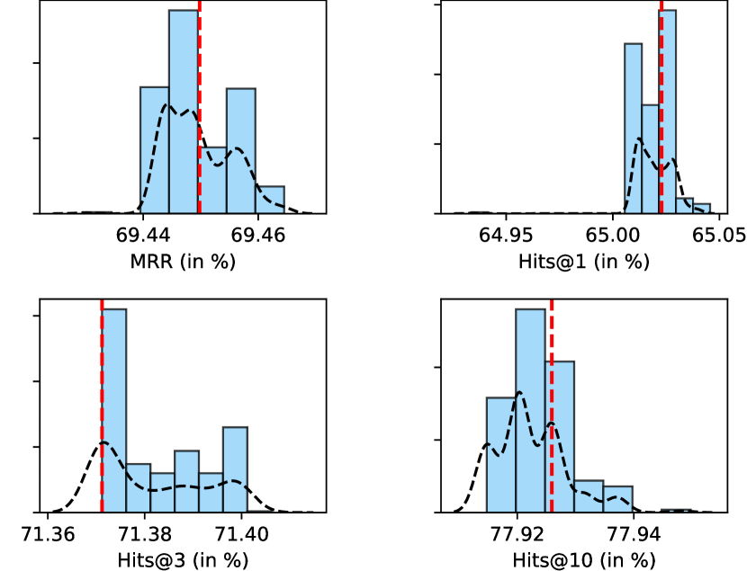
Figure 2: Distribution of performances of Hercules on temporally-corrupted quadruplets from ICEWS14 with dim=100. A smooth approximation of the distribution is drawn as a dashed black curve. The reference performance is indicated with a dashed red line.

We therefore assume that the optimization procedure may be involved. We consequently question the effect of negative sampling. Precisely, we train Hercules with dim = 40 by tuning the number of negative samples between 50 to 500. We plot the learning curves in Fig. 3.

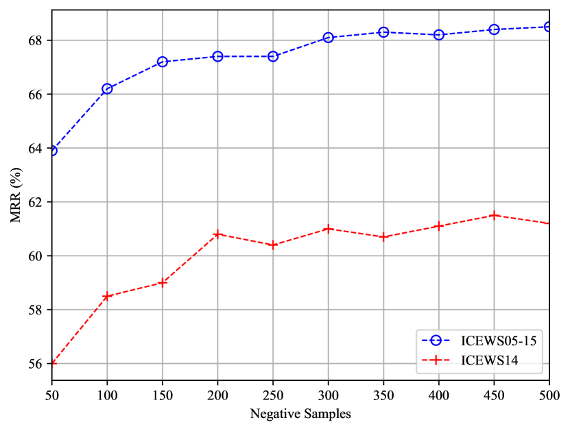
Figure 3: Performance of Hercules (dim = 40) on ICEWS14 and ICEWS05-15 with varying number of negative samples.

For both, ICEWS14 and ICEWS05-15, negative sampling shows considerable gain as the number of samples increases. We record an absolute gain of 5% points in MRR from 50 to 500 samples. We can see a rapid growth in MRR when the number of samples is inferior to 200. Adding 50 samples is equivalent to about 2% points gain in MRR. Then, performances reach a plateau around 300 negative samples. We conjecture that a diversity in negative samples is enough to learn good representations. Notwithstanding that a large number of negative samples heavily constraints the location of entities in space, the resulting embeddings might benefit from it to be better positioned relatively to others.

We conclude that despite the present time parameter, an optimal negative sampling enables to reach new state-of-the-art outcome. Therefore, we argue that time is not the only parameter that should be considered when performing LP. We highlight that one should be raising awareness when training TKG representations to identify if time is truly helping to boost performances.

6.4.3 AttH versus Hercules

We explore here how the geometry of Hercules differs from AttH. To do so, we inspect the absolute difference of their learned curvatures $\Delta_{c}$. We plot $\Delta_{c}$ with respect to the relations and timestamps for dim = 40 on ICEWS14 in Fig. 4. Similar plots are given for ICEWS05-15 in Appendix A.1.

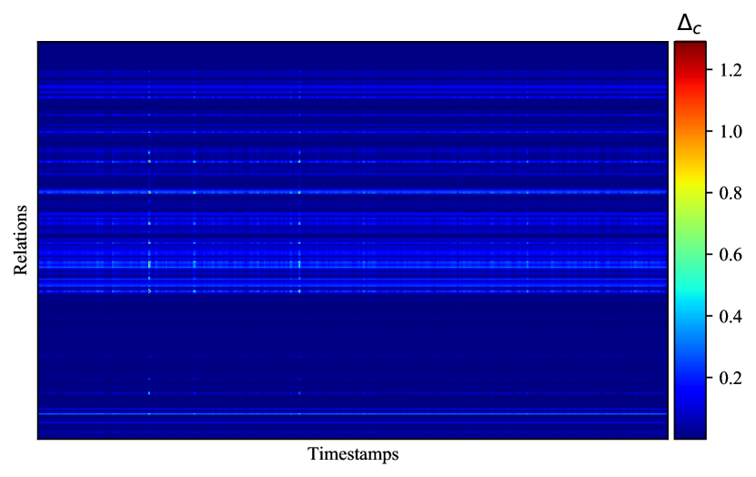
Figure 4: Absolute curvatures differences between AttH and Hercules given specific relation and time on ICEWS14 dataset (dim = 40).

Besides rare steep discrepancy in curvatures (i.e. $\Delta_{c}$ $>$ 1.0), Hercules is akin to AttH concerning learned geometries. We report that 85.0% and 95.6% of $\Delta_{c}$’s are smaller than 0.1 on ICEWS14 and ICEWS05-15 respectively. We point out that some timestamps affect globally all relations, albeit very limited. This can be seen in Fig. 5 by the aligned vertical strips. It indicates that Hercules uses its additional time parameter to learn a slightly different manifold but nonetheless quite similar to AttH. We provide further analysis on the shifts of the curvatures while increasing embeddings dimension in Appendices A.2 and A.3.

We depict an example of learned hyperbolic representation of ICEWS14 entities of AttH and Hercules for the relation ‘make a visit’and timestamp set to 01-01-2014 in Fig. 5. We plot embeddings of ICEWS05-15 in Appendix A.4.

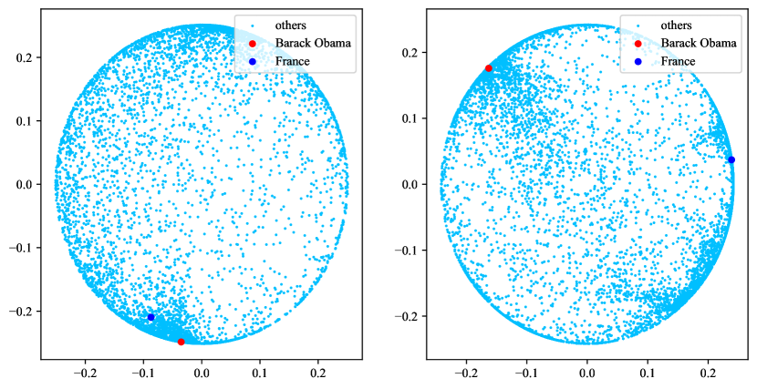
Figure 5: Illustration of two-dimensional hyperbolic entity embeddings learned by AttH (left) and Hercules (right) on ICEWS14 for predicate ‘make a visit’and timestamp set to 01-01-2014.

7 Conclusion

In this paper, we have demonstrated that without adding neither time information nor supplementary parameters, the AttH model astonishingly achieves similar or new state-of-the-art performances on link prediction upon temporal knowledge graphs. In spite of the inclusion of time with our proposed time-aware model Hercules, we have shown that negative sampling is sufficient to learn a good underlying geometry. In the future, we plan to explore new mechanisms to incorporate temporal information to improve performances of AttH.

Appendix A Appendices

A.1 AttH versus Hercules

We plot the absolute difference in curvatures between AttH and Hercules for dim = 40 on ICEWS05-15 in Fig. 6.

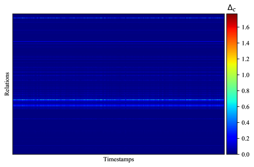
Figure 6: Absolute curvatures differences between AttH and Hercules given specific relation and time on ICEWS05-15 dataset (dim = 40).

As in ICEWS14 dataset, we observe that learned geometries on ICEWS15 dataset by AttH and Hercules are alike. Time is showing insubstantial impact on the curvature.

A.2 AttH versus AttH

We inspect how the curvature of AttH fluctuates while increasing the embedding dimension. We compare curvatures shifts between dim = 40 and dim = 100. We plot $\Delta_{c}$ in Fig. 7.

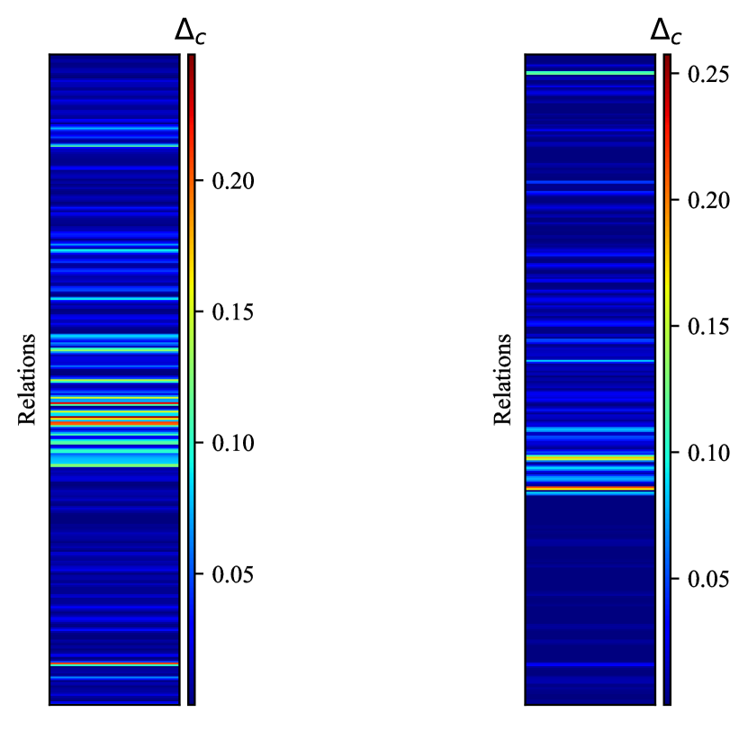
Figure 7: Absolute curvatures differences of AttH between dim = 40 and dim = 100 given specific relation and time on ICEWS14 dataset (left) and ICEWS05-15 dataset (right). No timestamps since AttH is a time-unaware model.

The fluctuation in curvature is moderate while dimension of embeddings increases. We can see that variation is almost inferior to 0.2. This underlines that geometry does not change much for a specific relation when the dimension grows. For some relations, we note however that curvature is knowing significant dissimilitudes.

A.3 Hercules versus Hercules

We report the dissimilarities in curvature for different relations and timestamps on ICEWS14 and ICEWS05-15 in Fig. 8 and Fig. 9.

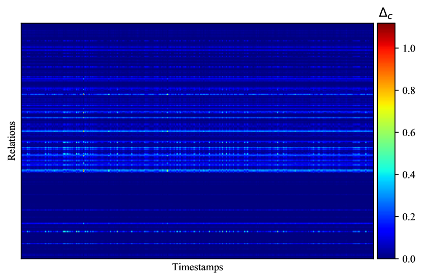
Figure 8: Absolute curvatures differences of Hercules between dim = 40 and dim = 100 given specific relation and time on ICEWS14 dataset.

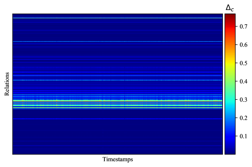
Figure 9: Absolute curvatures differences of Hercules between dim = 40 and dim = 100 given specific relation and time on ICEWS05-15 dataset.

We note that around 87.7% and 91.1% of variations are smaller than 0.1 on ICEWS14 and ICEWS05-15 respectively. This seems to indicate that despite the dimensionality gap, the learned geometry for each relation does not differ much between dim = 40 and dim = 100.

A.4 Two-Dimensional Hyperbolic Embeddings

We give an illustration of learned embeddings on ICEWS05-15 by AttH and Hercules models in Fig. 10.

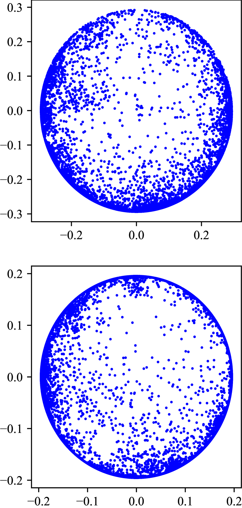
Figure 10: Illustration of two-dimensional hyperbolic embeddings learned by AttH (top) and Hercules (bottom) on ICEWS05-15.

References

- Balažević et al. (2019a) Ivana Balažević, Carl Allen, and Timothy Hospedales. 2019a. Multi-relational poincaré graph embeddings. In Advances in Neural Information Processing Systems.
- Balažević et al. (2019b) Ivana Balažević, Carl Allen, and Timothy Hospedales. 2019b. TuckER: Tensor factorization for knowledge graph completion. In Proceedings of the 2019 Conference on Empirical Methods in Natural Language Processing and the 9th International Joint Conference on Natural Language Processing (EMNLP-IJCNLP), pages 5185–5194, Hong Kong, China. Association for Computational Linguistics.
- Bonnabel (2013) Silvère Bonnabel. 2013. Stochastic gradient descent on riemannian manifolds. IEEE Transactions on Automatic Control, 58:2217–2229.
- Bordes et al. (2014) Antoine Bordes, Sumit Chopra, and Jason Weston. 2014. Question answering with subgraph embeddings. In Proceedings of the 2014 Conference on Empirical Methods in Natural Language Processing (EMNLP), pages 615–620, Doha, Qatar. Association for Computational Linguistics.
- Bordes et al. (2013) Antoine Bordes, Nicolas Usunier, Alberto Garcia-Durán, Jason Weston, and Oksana Yakhnenko. 2013. Translating embeddings for modeling multi-relational data. In Proceedings of the 26th International Conference on Neural Information Processing Systems - Volume 2, NIPS’13, page 2787–2795, Red Hook, NY, USA. Curran Associates Inc.
- Boschee et al. (2018) Elizabeth Boschee, Jennifer Lautenschlager, Sean O’Brien, Steve Shellman, and James Starz. 2018. ICEWS Weekly Event Data. Harvard Dataverse.
- Chami et al. (2020) Ines Chami, Adva Wolf, Da-Cheng Juan, Frederic Sala, Sujith Ravi, and Christopher Ré. 2020. Low-dimensional hyperbolic knowledge graph embeddings. In Proceedings of the 58th Annual Meeting of the Association for Computational Linguistics, pages 6901–6914, Online. Association for Computational Linguistics.
- Chami et al. (2019) Ines Chami, Zhitao Ying, Christopher Ré, and Jure Leskovec. 2019. Hyperbolic graph convolutional neural networks. In Advances in Neural Information Processing Systems, volume 32, pages 4868–4879. Curran Associates, Inc.
- Chen et al. (2020) Xiaojun Chen, Shengbin Jia, and Yang Xiang. 2020. A review: Knowledge reasoning over knowledge graph. Expert Systems with Applications, 141:112948.
- Dasgupta et al. (2018) Shib Sankar Dasgupta, Swayambhu Nath Ray, and Partha Talukdar. 2018. HyTE: Hyperplane-based temporally aware knowledge graph embedding. In Proceedings of the 2018 Conference on Empirical Methods in Natural Language Processing, pages 2001–2011, Brussels, Belgium. Association for Computational Linguistics.
- Ganea et al. (2018) Octavian Ganea, Gary Becigneul, and Thomas Hofmann. 2018. Hyperbolic neural networks. In Advances in Neural Information Processing Systems, volume 31, pages 5345–5355. Curran Associates, Inc.
- García-Durán et al. (2018) Alberto García-Durán, Sebastijan Dumančić, and Mathias Niepert. 2018. Learning sequence encoders for temporal knowledge graph completion. In Proceedings of the 2018 Conference on Empirical Methods in Natural Language Processing, pages 4816–4821, Brussels, Belgium. Association for Computational Linguistics.
- Goel et al. (2020) Rishab Goel, Seyed Mehran Kazemi, Marcus Brubaker, and Pascal Poupart. 2020. Diachronic embedding for temporal knowledge graph completion. In AAAI.
- Hamilton et al. (2016) William L. Hamilton, Jure Leskovec, and Dan Jurafsky. 2016. Diachronic word embeddings reveal statistical laws of semantic change. In Proceedings of the 54th Annual Meeting of the Association for Computational Linguistics (Volume 1: Long Papers), pages 1489–1501, Berlin, Germany. Association for Computational Linguistics.
- Han et al. (2020) Zhen Han, Peng Chen, Yunpu Ma, and Volker Tresp. 2020. DyERNIE: Dynamic Evolution of Riemannian Manifold Embeddings for Temporal Knowledge Graph Completion. In Proceedings of the 2020 Conference on Empirical Methods in Natural Language Processing (EMNLP), pages 7301–7316, Online. Association for Computational Linguistics.
- Hao et al. (2017) Yanchao Hao, Yuanzhe Zhang, Kang Liu, Shizhu He, Zhanyi Liu, Hua Wu, and Jun Zhao. 2017. An end-to-end model for question answering over knowledge base with cross-attention combining global knowledge. In Proceedings of the 55th Annual Meeting of the Association for Computational Linguistics (Volume 1: Long Papers), pages 221–231, Vancouver, Canada. Association for Computational Linguistics.
- Heath and Euclid (1956) Thomas L. Heath and Euclid. 1956. The Thirteen Books of Euclid’s Elements, Books 1 and 2. Dover Publications, Inc., USA.
- Hochreiter and Schmidhuber (1997) Sepp Hochreiter and Jürgen Schmidhuber. 1997. Long short-term memory. Neural computation, 9(8):1735–1780.
- Kingma and Ba (2014) Diederik P. Kingma and Jimmy Ba. 2014. Adam: A method for stochastic optimization. Cite arxiv:1412.6980Comment: Published as a conference paper at the 3rd International Conference for Learning Representations, San Diego, 2015.
- Lao and Cohen (2010) Ni Lao and William W. Cohen. 2010. Relational retrieval using a combination of path-constrained random walks. Mach. Learn., 81(1):53–67.
- Leblay and Chekol (2018) Julien Leblay and Melisachew Wudage Chekol. 2018. Deriving validity time in knowledge graph. In Companion Proceedings of the The Web Conference 2018, WWW ’18, page 1771–1776, Republic and Canton of Geneva, CHE. International World Wide Web Conferences Steering Committee.
- Lin et al. (2015) Yankai Lin, Zhiyuan Liu, Maosong Sun, Yang Liu, and Xuan Zhu. 2015. Learning entity and relation embeddings for knowledge graph completion. In Proceedings of the Twenty-Ninth AAAI Conference on Artificial Intelligence, AAAI’15, page 2181–2187. AAAI Press.
- Liu et al. (2019) Qi Liu, Maximilian Nickel, and Douwe Kiela. 2019. Hyperbolic graph neural networks. In Advances in Neural Information Processing Systems, volume 32, pages 8230–8241. Curran Associates, Inc.
- Ma et al. (2019) Yunpu Ma, Volker Tresp, and Erik A. Daxberger. 2019. Embedding models for episodic knowledge graphs. Journal of Web Semantics, 59:100490.
- Nickel and Kiela (2017) Maximilian Nickel and Douwe Kiela. 2017. Poincaré embeddings for learning hierarchical representations. In I. Guyon, U. V. Luxburg, S. Bengio, H. Wallach, R. Fergus, S. Vishwanathan, and R. Garnett, editors, Advances in Neural Information Processing Systems 30, pages 6341–6350. Curran Associates, Inc.
- Nickel and Tresp (2013) Maximilian Nickel and Volker Tresp. 2013. Tensor factorization for multi-relational learning. In Machine Learning and Knowledge Discovery in Databases, pages 617–621, Berlin, Heidelberg. Springer Berlin Heidelberg.
- Rocktäschel et al. (2015) Tim Rocktäschel, Sameer Singh, and Sebastian Riedel. 2015. Injecting logical background knowledge into embeddings for relation extraction. In Proceedings of the 2015 Conference of the North American Chapter of the Association for Computational Linguistics: Human Language Technologies, pages 1119–1129, Denver, Colorado. Association for Computational Linguistics.
- Sarkar (2011) Rik Sarkar. 2011. Low distortion delaunay embedding of trees in hyperbolic plane. In Proceedings of the 19th International Conference on Graph Drawing, GD’11, page 355–366, Berlin, Heidelberg. Springer-Verlag.
- Saxena et al. (2020) Apoorv Saxena, Aditay Tripathi, and Partha Talukdar. 2020. Improving multi-hop question answering over knowledge graphs using knowledge base embeddings. In Proceedings of the 58th Annual Meeting of the Association for Computational Linguistics, pages 4498–4507, Online. Association for Computational Linguistics.
- Sun et al. (2019) Zhiqing Sun, Zhi-Hong Deng, Jian-Yun Nie, and Jian Tang. 2019. Rotate: Knowledge graph embedding by relational rotation in complex space. In International Conference on Learning Representations.
- Trivedi et al. (2017) Rakshit Trivedi, Hanjun Dai, Yichen Wang, and Le Song. 2017. Know-evolve: Deep temporal reasoning for dynamic knowledge graphs. In Proceedings of the 34th International Conference on Machine Learning - Volume 70, ICML’17, page 3462–3471. JMLR.org.
- Trouillon et al. (2016) Théo Trouillon, Johannes Welbl, Sebastian Riedel, Éric Gaussier, and Guillaume Bouchard. 2016. Complex embeddings for simple link prediction. In Proceedings of the 33rd International Conference on International Conference on Machine Learning - Volume 48, ICML’16, page 2071–2080. JMLR.org.
- Vermeer (2005) J. Vermeer. 2005. A geometric interpretation of ungar’s addition and of gyration in the hyperbolic plane. Topology and its Applications, 152(3):226 – 242. Special Issue Jan Aarts.
- Wang et al. (2014) Zhen Wang, Jianwen Zhang, Jianlin Feng, and Zheng Chen. 2014. Knowledge graph embedding by translating on hyperplanes. In Proceedings of the Twenty-Eighth AAAI Conference on Artificial Intelligence, AAAI’14, page 1112–1119. AAAI Press.
- Xian et al. (2019) Yikun Xian, Zuohui Fu, S. Muthukrishnan, Gerard de Melo, and Yongfeng Zhang. 2019. Reinforcement knowledge graph reasoning for explainable recommendation. In Proceedings of the 42nd International ACM SIGIR Conference on Research and Development in Information Retrieval, SIGIR’19, page 285–294, New York, NY, USA. Association for Computing Machinery.
- Xiong et al. (2017) Chenyan Xiong, Russell Power, and Jamie Callan. 2017. Explicit semantic ranking for academic search via knowledge graph embedding. In Proceedings of the 26th International Conference on World Wide Web, WWW ’17, page 1271–1279, Republic and Canton of Geneva, CHE. International World Wide Web Conferences Steering Committee.
- Xu et al. (2019) Chengjin Xu, Mojtaba Nayyeri, Fouad Alkhoury, Jens Lehmann, and Hamed Shariat Yazdi. 2019. Temporal knowledge graph embedding model based on additive time series decomposition. arXiv preprint arXiv:1911.07893.
- Xu et al. (2020a) Chengjin Xu, Mojtaba Nayyeri, Fouad Alkhoury, Hamed Shariat Yazdi, and Jens Lehmann. 2020a. TeRo: A time-aware knowledge graph embedding via temporal rotation. In Proceedings of the 28th International Conference on Computational Linguistics, pages 1583–1593, Barcelona, Spain (Online). International Committee on Computational Linguistics.
- Xu et al. (2020b) Chengjin Xu, Mojtaba Nayyeri, Fouad Alkhoury, Hamed Shariat Yazdi, and Jens Lehmann. 2020b. Tero: A time-aware knowledge graph embedding via temporal rotation. arXiv preprint arXiv:2010.01029.
- Yang et al. (2015) Bishan Yang, Scott Wen-tau Yih, Xiaodong He, Jianfeng Gao, and Li Deng. 2015. Embedding entities and relations for learning and inference in knowledge bases. In Proceedings of the International Conference on Learning Representations (ICLR) 2015.
- Yu et al. (2014) Xiao Yu, Xiang Ren, Yizhou Sun, Quanquan Gu, Bradley Sturt, Urvashi Khandelwal, Brandon Norick, and Jiawei Han. 2014. Personalized entity recommendation: A heterogeneous information network approach. In Proceedings of the 7th ACM International Conference on Web Search and Data Mining, WSDM ’14, page 283–292, New York, NY, USA. Association for Computing Machinery.
- Zhang et al. (2016) Fuzheng Zhang, Nicholas Jing Yuan, Defu Lian, Xing Xie, and Wei-Ying Ma. 2016. Collaborative knowledge base embedding for recommender systems. In Proceedings of the 22nd ACM SIGKDD International Conference on Knowledge Discovery and Data Mining, KDD ’16, page 353–362, New York, NY, USA. Association for Computing Machinery.
- Zhang et al. (2019) Shuai Zhang, Yi Tay, Lina Yao, and Qi Liu. 2019. Quaternion knowledge graph embedding. arXiv preprint arXiv:1904.10281.
- Zhou et al. (2017) Chang Zhou, Yuqiong Liu, Xiaofei Liu, Zhongyi Liu, and Jun Gao. 2017. Scalable graph embedding for asymmetric proximity. Proceedings of the AAAI Conference on Artificial Intelligence, 31(1).