Spectrally-wide acoustic frequency combs generated using oscillations of polydisperse gas bubble clusters in liquids

Abstract

Acoustic frequency combs leverage unique properties of the optical frequency comb technology in high-precision measurements and innovative sensing in optically inaccessible environments such as under water, under ground or inside living organisms. Because acoustic combs with wide spectra would be required for many of these applications but techniques of their generation have not yet been developed, here we propose a new approach to the creation of spectrally-wide acoustic combs using oscillations of polydisperse gas bubble clusters in liquids. By means of numerical simulations we demonstrate that clusters consisting of bubbles with precisely controlled sizes can produce wide acoustic spectra composed of equally-spaced coherent peaks. We show that under typical experimental conditions bubble clusters remain stable over time required for a reliable recording of comb signals. We also demonstrate that the spectral composition of combs can be tuned by adjusting the number and size of bubbles in a cluster.

I Introduction

Frequency combs (FCs) are spectra containing equidistant coherent peaks. Although mostly optical FCs have found widespread practical and fundamental applications so far [1, 2], in general FCs can be generated using waves other than light. For example, a number of acoustic, phononic and acousto-optical FC techniques have recently been introduced [3, 4, 5, 6, 7, 8, 9, 10, 11, 12, 13]. Among them, the acoustic frequency comb (AFC) techniques stand out because they hold the promise to enable ultrasensitive vibration detectors [14], phonon lasers [15, 16] and quantum computers [17]. AFCs can also find applications in precision measurements in diverse physical, chemical and biological systems in conditions, where using light—and hence optical FCs—poses technical and fundamental limitations. For example, this is the case in under-water distance measurements [9] and also in some biomedical imaging modalities [3, 6, 10].

In our previous work [13], we have theoretically and experimentally demonstrated the possibility of generating AFCs using oscillations of a cluster of gas bubbles in liquids [18, 19, 20]. We used low-pressure harmonic ultrasound signals with the frequency that is an order of magnitude higher than the natural frequency of the bubble cluster [21, 19]. The interaction of ultrasound waves with an oscillating bubble at the natural frequency of a cluster results in the amplitude modulation of cluster’s response and the appearance of sidebands around the harmonic and ultraharmonic peaks of the driving ultrasound wave. We demonstrated that such sideband structures can be used as AFCs.

However, as with other AFC generation techniques [6, 8], in our experiments the number of sideband peaks usable as an AFC is small. At present, this restriction presents numerous technological challenges that shape research efforts in the field of FCs [1, 2]. For example, similarly to optical FCs, for many applications the AFC spectrum has to span over an octave of a bandwidth—that is, the highest frequency in the comb spectrum has to be at least twice the lowest frequency. Of course, the spectrum of an AFC can be extended using one of the techniques developed, for example, for broadening the spectra of opto-electronic FCs [22] such as supercontinuum generation using nonlinear optical effects. (here, the adoption of optical techniques in the acoustic domain is possible because of the analogy between nonlinear optical processes in photonic devices and nonlinear acoustic processes in liquids containing gas bubbles [10].) Furthermore, our analysis reported in [13] demonstrates that the number of peaks in a bubble-generated AFC and their relative magnitude can be increased by simultaneously decreasing the frequency and increasing the pressure of the ultrasound wave driving bubble oscillations.

In the current work, we suggest an alternative strategy for broadening spectra of AFCs generated using oscillations of gas bubbles. We theoretically investigate the use of polydisperse clusters consisting of mm-sized bubbles with equilibrium radii $R_{n0}=R_{10}/n$, where $R_{10}$ is the equilibrium radius of the largest bubble in the cluster and $n=1,2,3,\ldots$ is the number of bubbles in the cluster. Although clusters with other bubble size distributions could be used in the proposed approach, the specific ratio of equilibrium radii investigated in this paper allows generating AFCs with a quasi-continuum of equally-spaced peaks, which is convincingly demonstrated below by numerical simulations of clusters with $n=4$ bubbles. In line with our previous experiments [13], in our analysis we consider low-pressure ultrasound waves (up to 10 kPa). We show that the ultrasound frequency can be chosen in a wide spectral range above the natural oscillation frequency of individual bubbles in the cluster. Our calculations demonstrate that these relaxed technical specifications can greatly facilitate the generation and recording of stable AFC signals. This is because at low pressure insonification bubble clusters exhibit a regular behaviour until the bubble dynamics becomes affected by their aggregation [13]. Moreover, formation a bubble cluster with mm-range equilibrium radii of about $2/n$ mm is technologically straightforward and can be accomplished using only a simple bubble generator equipped with a customised air diffuser [13].

It is noteworthy that stable gas bubble clusters called bubble grapes have been previously generated [23, 24, 25, 26] using low-pressure ultrasound waves. However, as discussed in Sec. II, bubble grapes are formed when the sign of the secondary Bjerknes force is reversed and the corresponding equilibrium state becomes stable [27]. In contrast, we propose to generate AFCs in a regime, where the bubbles attract each other but the magnitude of the secondary Bjerknes force is very small due to the disparate natural bubble frequencies and the frequency of the driving ultrasound wave. As a result, the inter-bubble distance and the overall arrangement of bubbles within a cluster appear to be sufficiently stable for the observation of well-pronounced AFC spectra without applying any additional cluster stabilisation procedures.

II Background theory

The accepted model of nonlinear oscillations of a single gas bubble that does not undergo translational motion is given by the Keller-Miksis (KM) equation [28] that takes into account the decay of bubble oscillations due to viscous dissipation and fluid compressibility. However, when the focus is on mm-sized gas bubbles oscillating at 20–100 kHz frequencies in water being driven by low-pressure ultrasound waves (with the amplitude of up to 10 kPa), the terms in the KM equation accounting for acoustic losses become negligible [13]. Thus, the KM equation effectively reduces to the classical Rayleigh-Plesset (RP) equation [29, 30].

As with a single bubble, the RP equation for a cluster consisting of $N$ bubbles not undergoing translational motion can be obtained by removing the acoustic losses terms from the generalised KM equation for a bubble cluster [31, 32]:

$$R_{n}\frac{d^{2}R_{n}}{dt^{2}} + \frac{3}{2}\left(\frac{dR_{n}}{dt}\right)^{2}$$ (1)

$$= \frac{1}{\rho}\left(P\left(R_{n},\frac{dR_{n}}{dt}\right)-P_{\infty}(t)\right)-P_{sn}\,,$$

where

$$P_{n}\left(R_{n},\frac{dR_{n}}{dt}\right) = \left(P_{0}-P_{v}+\frac{2\sigma}{R_{n0}}\right)\left(\frac{R_{n0}}{R_{n}}\right)^{3\kappa}$$ (2)

$$-\frac{4\mu}{R_{n}}\frac{dR_{n}}{dt}-\frac{2\sigma}{R_{n}}\,.$$

The term accounting for the pressure acting on of the $n$th bubble due to scattering of the incoming pressure wave by the neighbouring bubbles in a cluster is given by

$$P_{sn}=\sum_{l=1,l\neq n}^{N}\dfrac{1}{d_{nl}}\left(R_{l}^{2}\frac{d^{2}R_{l}}{dt^{2}}+2R_{l}\left(\frac{dR_{l}}{dt}\right)^{2}\right)\,,$$ (3)

where $d_{nl}$ is the inter-bubble distance and $N$ is the total number of bubbles in the cluster. The expression $P_{\infty}(t)=P_{0}-P_{v}+\alpha\sin(\omega^{*}t)$ with the angular frequency $\omega^{*}=2\pi f$ represents the periodically varied pressure in the liquid far from the bubble. Parameters $R_{n0}$, $R_{n}(t)$, $\mu$, $\rho$, $\kappa$, $\sigma$, $\alpha$ and $f$ denote the equilibrium and instantaneous radii of the $n$th bubble in the cluster, the dynamic viscosity and the density of the liquid, the polytropic exponent of a gas entrapped in the bubble, the surface tension of a gas-liquid interface and the amplitude and the frequency of a driving ultrasound wave. Diffusion of the gas through the bubble surface is neglected.

When bubble oscillations are not affected by fluid compressibility, which is the case in this work, the acoustic power scattered by the $n$th bubble in the cluster in the far-field zone is [18]

$$P_{scat}(R_{n},t)=\frac{\rho R_{n}}{h}\left(R_{n}\ddot{R}_{n}+2\dot{R}_{n}^{2}\right)\,,$$ (4)

where $h$ is much larger than the spatial extent of the cluster.

Interactions of gas bubbles, including their radial oscillations and translational motion driven by an acoustic pressure field, has been a subject of intensive research (see, e.g., [33, 27, 34, 35, 36, 31, 37, 38, 39, 40, 41, 42, 43, 44, 45, 32, 46, 47]; for a review see [48]). Most of these works are based on the accepted models of spherical gas bubble oscillations [Eqs. (1)–(3)] and account for the action of Bjerknes forces [49]. The primary Bjerknes force $F_{pB}$ is caused by the acoustic pressure field [49, 50] while the secondary Bjerknes force $F_{sB}$ arises between two and more bubbles in the same pressure field [48]. The secondary Bjerknes force between two gas bubbles is repulsive when the driving frequency lies between the natural frequencies of the bubbles, otherwise it is attractive [48]. This theoretical prediction was confirmed experimentally [51, 52].

However, several important experimental observations cannot be explained using Bjerknes theory. These include the formation of stable bubble grape clusters [23, 25] and self-organisation effects in bubble-liquid mixtures [53] that explain acoustic streaming phenomena [39, 54] and underpin some techniques of bubble manipulation [46].

Kobelev and co-workers [23] were the first to report the formation of bubble grapes as a byproduct of their experiment targeting the attenuation of sound in liquids containing gas bubbles. They demonstrated that nonlinear oscillations of gas bubbles can not be responsible for the observed effect. The original Bierknes force theory [49, 50, 48] based on the linear oscillations of gas bubbles is unable to explain this phenomenon either since (i) it applies only to gas bubbles separated by distances that are much larger then the bubble radii and (ii) it only predicts whether the bubbles attract or repulse depending on their natural frequencies. Thus, the only plausible explanation of the formation of bubble grapes could be a reversal in the secondary Bjerknes force from attractive to repulsive.

One of the first attempts to theoretically explain the formation of bubble grapes was made by Nemtsov [33]. However, his model did not account for wave scattering by bubbles [48]. Zabolotskaya [27] was first to develop a model explaining the sign reversal of the secondary Bjerknes force. Ozug and Prosperetti [55] theoretically demonstrated the possibility of sign reversal of the secondary Bjerknes force in the case of nonlinear bubble oscillations driven by high-pressure acoustic waves. However, the result presented in their work cannot explain linear processes underlying the formation of bubble grapes. Subsequently, Zabolotskaya’s theory was extended by Doinikov and Zavtrak [48] and used to explain [25] an intriguing observation of stable bubble structures in an experiment involving strongly forced mm-sized gas bubbles oscillating in low gravity conditions [24]. An alternative interpretation of the sign reversal of the secondary Bjerknes force was proposed in [56].

However, although the experimental conditions in our work reported in [13] indeed resemble those required for the formation of bubble grapes, the bubble clusters we observed form due to a different mechanism that does not involve the sign reversal of Bjerknes force. This is because we use mm-size bubble with the natural frequencies of 1–3 kHz but drive their oscillations with a low-pressure high-kHz-range ultrasound. As a result, although the aggregation and eventual coalescence of bubble are inevitable in our experiments, they occur on a timescale of several seconds and hence are mostly inconsequential for the generation of AFCs.

III Interaction between two gas bubbles

The interaction dynamics of gas bubbles oscillating in liquids is very complex because the cluster geometry varies from experiment to experiment and with time. Therefore, many theoretical works consider a system of just two interacting bubbles surrounded by an idealised liquid. This simplification allows reducing the complexity of the model while accounting for the essential physics of bubble interaction.

III.1 Analysis of the RP equation for two interacting gas bubbles

To identify the main characteristics of nonlinear oscillations of interacting gas bubbles relevant to the generation of AFCs, we conduct an asymptotic analysis of Eq. (1) extending our previous model of nonlinear oscillations of a single gas bubble [13].

We start with rewriting Eq. (1) in the non-dimensional form using the equilibrium radius of the largest bubble in the cluster, $R_{10}$, and $1/{\omega^{*}}$ as the length and time scales, respectively, to introduce the non-dimensional quantities $r_{n}={R_{n}(t)}/R_{10}$, $r_{l}={R_{l}(t)}/R_{10}$ and $\tau^{*}=\omega^{*}t$ [32]. Substituting these into Eq. (1) we obtain

$$r_{n}{r_{n}}^{\prime\prime} + \frac{3}{2}{{r_{n}}^{\prime}}^{2}=\left({\cal M}+\frac{{\cal W}}{{\cal Q}_{n}}\right)\left(\frac{{\cal Q}_{n}}{r_{n}}\right)^{\cal K}-\frac{{\cal W}}{r_{n}}-{\cal R}\frac{{r_{n}}^{\prime}}{r_{n}}$$ (5)

$$- {\cal M}-{\cal M}_{e}\sin\tau^{*}-\sum_{\begin{subarray}{c}l=1\\ l\neq n\end{subarray}}^{N}\zeta_{nl}\left(r_{l}^{2}r_{l}^{\prime\prime}+2r_{l}{r_{l}^{\prime}}^{2}\right)\,,$$

where ${\cal R}=\dfrac{4\mu}{\rho\omega^{*}R^{2}_{10}}$, ${\cal W}=\dfrac{2\sigma}{\rho\omega^{*2}R^{3}_{10}}$, ${\cal M}=\dfrac{P_{0}-P_{v}}{\rho\omega^{*2}R^{2}_{10}}$, ${\cal M}_{e}=\dfrac{\alpha}{\rho\omega^{*2}R^{2}_{10}}$, $\zeta_{nl}=\dfrac{R_{10}}{d_{nl}}$, ${\cal K}=3\kappa$ and ${\cal Q}_{n}=\dfrac{R_{n0}}{R_{10}}$. Parameter ${\cal M}$ characterises elastic properties of the gas and its compressibility, ${\cal W}$ and ${\cal R}$ can be treated as inverse Weber and Reynolds numbers, representing the surface tension and viscous dissipation effects, respectively, and ${\cal M}_{e}$ is the measure of the ultrasound forcing [57]. Parameters $\zeta_{nl}$ and ${\cal Q}_{n}$ are the inverse of the distance between the bubble centres and the bubble radius relative to that of the largest bubble in the cluster, respectively [32] and primes denote differentiation with respect to $t$. As discussed in [57, 13], ${\cal K}=4$ for bubbles of sizes relevant to the AFC context and for the fluid parameters, ultrasound pressure and frequency given in Sec. IV the maximum values of other parameters do not exceed ${\cal M}=9.7\times 10^{-4}$, ${\cal W}=7.4\times 10^{-7}$, ${\cal R}=6.5\times 10^{-6}$ and ${\cal M}_{e}=9.9\times 10^{-5}$. Therefore, the effects of water viscosity and surface tention on bubble oscillations are negligible and we set ${\cal R}={\cal W}=0$ in what follows. Thus, ultrasonically forced bubble oscillations can be assumed perfectly periodic when the driving frequency is much higher than any of the natural frequencies of the individual bubbles in the cluster (i.e. no resonances arises). This warrants using a method similar to that in [13].

We consider a cluster consisting of two gas bubbles with the non-dimensional equilibrium radii $r_{n0}={\cal Q}_{n}$, $n=1,2$ (${\cal Q}_{1}\equiv 1$). Following [58, 13] we look for the asymptotic solutions of Eq. (5) in the form

$$r_{n}={\cal Q}_{n}+\epsilon r_{n1}(\tau)+\epsilon^{2}r_{n2}(\tau)+\ldots\,,\quad n=1,2\,,\\$$ (6)

where $0<\epsilon\ll 1$ is a parameter characterising the amplitude of bubble oscillations used to distinguish between various terms in the asymptotic series and $\tau=\omega\tau^{*}=\omega\omega^{*}t$. At the first order of $\epsilon$ we obtain

$$\ddot{r}_{11}+\frac{{\cal K}{\cal M}}{{\cal Q}_{1}^{2}\omega^{2}}r_{11}+\frac{{\cal Q}_{2}^{2}}{{\cal Q}_{1}}\zeta_{12}\ddot{r}_{21}=\frac{p}{{\cal Q}_{1}}\sin(\Omega\tau)\,,$$ (7)

$$\ddot{r}_{21}+\frac{{\cal K}{\cal M}}{{\cal Q}_{2}^{2}\omega^{2}}r_{21}+\frac{{\cal Q}_{1}^{2}}{{\cal Q}_{2}}\zeta_{12}\ddot{r}_{11}=\frac{p}{{\cal Q}_{2}}\sin(\Omega\tau)\,,$$ (8)

where overdots denote differentiation with respect to $\tau$ and we write $({\cal M}_{e}/\omega^{2})\sin{\tau^{*}}\equiv-\epsilon p\sin(\Omega\tau)$ and introduce $\Omega\equiv 1/\omega\gg 1$. For convenience we also choose $\omega^{2}={\cal K}{\cal M}$, where ${\cal K}{\cal M}$ is Minnaert frequency [21, 13] of the largest bubble in the cluster. Finally, we obtain

$$\ddot{r}_{11}+r_{11}+{\cal Q}_{2}^{2}\zeta_{12}\ddot{r}_{21}=p\sin(\Omega\tau)\,,$$ (9)

$$\ddot{r}_{21}+\frac{1}{{\cal Q}_{2}^{2}}r_{21}+\frac{\zeta_{12}}{{\cal Q}_{2}}\ddot{r}_{11}=\frac{p}{{\cal Q}_{2}}\sin(\Omega\tau)\,.$$ (10)

At ${\cal O}(\epsilon^{2})$ equations then become:

$$\ddot{r}_{12}+r_{12}+{\cal Q}_{2}^{2}\zeta_{12}\ddot{r}_{22} = \frac{{\cal K}+1}{2}r_{11}^{2}-\frac{3}{2}\dot{r}_{11}^{2}-r_{11}\ddot{r}_{11}$$ (11)

$$-2{\cal Q}_{2}\zeta_{12}\left(\dot{r}_{21}^{2}+r_{21}\ddot{r}_{21}\right)\,,$$

$$\ddot{r}_{22}+\frac{1}{{\cal Q}_{2}^{2}}r_{22}+\frac{\zeta_{12}}{{\cal Q}_{2}}\ddot{r}_{12} = \frac{{\cal K}+1}{{\cal Q}_{2}^{2}}r_{21}^{2}-\frac{3}{2{\cal Q}_{2}}\dot{r}_{21}^{2}-\frac{1}{{\cal Q}_{2}}{r}_{21}\ddot{r}_{21}$$ (12)

$$-2\frac{\zeta_{12}}{{\cal Q}_{2}}\left(\dot{r}_{11}^{2}+r_{11}\ddot{r}_{11}\right)\,.$$

Similarly to [13] we write the random initial conditions as $r_{1}(0)=1+\epsilon a$, $r_{2}(0)={\cal Q}_{2}+\epsilon b$, $\dot{r_{1}}(0)=\epsilon c$ and $\dot{r_{2}}(0)=\epsilon d$ that results in

$$r_{11}(0)=a,\ r_{21}(0)=b,\ \dot{r}_{11}(0)=c,\ \dot{r}_{21}(0)=d\,.$$ (13)

Subsequently, we obtain the leading order solutions

$$r_{11}(\tau) = C_{1}\cos{(\omega^{\prime}_{1}\tau+\phi_{1})}+C_{2}\cos{(\omega^{\prime}_{2}\tau+\phi_{2})}$$ (14)

$$+B_{1}\sin{\Omega\tau}\,,$$

$$r_{21}(\tau) = C_{3}\cos{(\omega^{\prime}_{1}\tau+\phi_{1})}+C_{4}\cos{(\omega^{\prime}_{2}\tau+\phi_{2})}$$ (15)

$$+B_{2}\sin{\Omega\tau}\,,$$

where $\omega^{\prime}_{1,2}=\dfrac{\sqrt{2}}{\sqrt{{\cal Q}_{2}^{2}+1\pm\sqrt{({\cal Q}_{2}^{2}-1)^{2}+4{\cal Q}_{2}^{3}\zeta_{12}^{2}}}}$. These frequencies depend on the inverse of the inter-bubble distance $\zeta_{12}$, which is a well-established fact [27, 48, 59]. Considering a particular case of ${\cal Q}_{2}=\frac{1}{2}$, as expected, for non-interacting distant bubbles with $\zeta_{12}\rightarrow 0$ we obtain $\omega^{\prime}_{1}\to\omega^{\prime}_{10}=1$ and $\omega^{\prime}_{2}\to\omega^{\prime}_{20}=2$. In general, the leading order bubble response will always contain three distinct frequencies: two bubble’s natural frequencies $\omega^{\prime}_{1,2}$ and the driving ultrasound frequency $\Omega$.

Coefficients $C_{1-4}$ and phase shifts $\phi_{1,2}$ in Eqs (14) and (15) depend on $\zeta_{12}$, $\Omega$ and $p$. As shown in [13] their exact expressions can be obtained for arbitrary initial conditions (13). However, the resulting expressions are too long to be given here explicitly and we only discuss the physical conclusions that follow from them. Specifically, these coefficients demonstrate that the spectra of both bubbles contain frequencies $\Omega$ and $\omega^{\prime}_{1,2}$. The magnitude of the $\omega_{1}^{\prime}$ peak is greater than that of $\omega_{2}^{\prime}$ in the spectrum of bubble 1 and vice versa. In the spectra of both bubbles, the amplitude of the peak corresponding to the frequency of a neighbouring bubble decreases with the distance between them and vanishes when the interaction between them becomes negligible.

Analysis of Eqs (10) and (12) can be performed following the procedure outlined in [13]. However, here we do not pursuit this any further since for the purposes of the current work it suffices to note that the right-hand sides of these equations contain quadratic terms involving $r_{11}$ and $r_{12}$ and their derivatives. Therefore, in addition to the harmonic components with frequencies $\omega^{\prime}_{1,2}$ solutions of Eqs (10) and (12) will include steady and periodic terms with frequencies equal to all possible pair-wise sums and differences of $\omega^{\prime}_{1,2}$ and $\Omega$: $\omega^{\prime}_{1,2}\pm\omega^{\prime}_{2,1}$, $\Omega\pm\omega^{\prime}_{1,2}$, $2\omega_{1,2}^{\prime}$ and $2\Omega$.

III.2 Bjerknes force between two oscillating bubbles

The asymptotic analysis in Sec. III.1 shows that, when the bubble oscillations are driven by a low-pressure ultrasound wave, the magnitude of any nonlinear effects is proportional to ${\cal M}_{e}^{2}\sim 9.8\times 10^{-9}$ (as per experimental conditions in [13]). Hence, the nonlinearity is neglected in this section.

Two physically equivalent dimensional expressions accounting for a sign reversal of Bjerknes force arising between two oscillating gas bubbles separated by a distance that is much larger than bubble radii were derived previously in [27] and [48]. From the expression given by Eq. (2.5) in [48] we obtain the leading term of the non-dimensional secondary Bjerknes force (scaled with $\rho{\omega^{*}}^{2}R_{10}^{4}$)

$$F^{\prime}_{sB}=-4\pi\zeta_{12}^{2}{\cal Q}_{2}^{2}\omega^{2}\epsilon^{2}\langle r_{11}\ddot{r}_{21}\rangle\,,$$ (16)

where the angle brackets denote time averaging. Substituting expressions (14) and (15) into Eq. (16), taking into account that $\left|\omega_{1}^{\prime}-\omega_{2}^{\prime}\right|\sim 1$ we obtain

$$F^{\prime}_{sB}=2\pi\zeta_{12}^{2}Q_{2}^{2}\omega^{2}\epsilon^{2}\left(B_{1}B_{2}\Omega^{2}+C_{1}C_{3}{\omega_{1}^{\prime}}^{2}+C_{2}C_{4}{\omega_{2}^{\prime}}^{2}\right)\,.$$

Evaluating coefficients $B_{1,2}$ and $C_{1-4}$ in the limit $\zeta_{12}\to 0$ finally leads to

$$F^{\prime}_{sB}=4\pi\zeta_{12}^{2}{\cal Q}_{2}^{2}{\cal M}_{e}^{2}\frac{\Omega^{8}}{(\Omega-1)^{2}(\Omega+1)^{2}}\,.$$ (17)

Here we focus on a particular bubble oscillation regime [13] characterised by $\Omega\gg 1$. In this case

$$F^{\prime}_{sB}\to 4\pi\zeta_{12}^{2}{\cal Q}_{2}^{2}{\cal M}_{e}^{2}\Omega^{4}=4\pi\zeta_{12}^{2}{\cal Q}_{2}^{2}\frac{{\cal M}_{e}^{2}}{{\cal K}^{2}{\cal M}^{2}}\,.$$ (18)

By its definition, $Q_{2}<1$ and in the reference experiment [13] ${\cal M}_{e}/({\cal K}{\cal M})\sim 0.025$ and $\zeta_{12}^{2}\lesssim 0.04$. Therefore, we conclude that the secondary Bjerknes force is small at the typical driving frequencies used in the generation of bubble-based AFCs away from bubble resonances. This provides an opportunity for measuring the acoustic bubble response and recording the resulting signals for AFC applications before bubble oscillations become affected by their aggregation. Our calculations using a more rigorous model of a translational motion, the results of which are presented in Sec. IV, provide convincing arguments in favour of this.

III.3 Dynamics of multi-bubble clusters with translational motion

It has been shown in [61] that Eq. (1) can be extended to include the effect of a translational bubble motion. The resulting system of differential equations reads

$$R_{n}\ddot{R}_{n}+\frac{3}{2}\dot{R}_{n}^{2}-\frac{P_{n}}{\rho}=\frac{\dot{\bf{p}}_{n}}{4}-\sum\limits_{\begin{subarray}{c}l=1\\ l\neq n\end{subarray}}^{N}\left\{\frac{R_{l}^{2}\ddot{R}_{l}+2R_{l}\dot{R}_{l}^{2}}{d_{nl}}\right.$$

$$\qquad+\frac{R_{l}^{2}}{2d_{nl}^{3}}({\bf p}_{n}-{\bf p}_{l})\cdot(R_{l}\ddot{\bf p}_{l}+\dot{R}_{l}\dot{\bf p}_{n}+5\dot{R}_{l}\dot{\bf p}_{l})$$

$$\qquad-\frac{R_{l}^{3}}{4d_{nl}^{3}}\Big{[}\dot{\bf p}_{l}\cdot(\dot{\bf{p}}_{n}+2\dot{\bf p}_{l})$$

$$\qquad+\frac{3}{d_{nl}^{2}}[\dot{\bf{p}}_{l}\cdot({\bf{p}}_{l}-{\bf p}_{n})][({\bf p}_{n}-{\bf p}_{l})\cdot(\dot{\bf p}_{n}+2\dot{\bf p}_{l})]\Big{]}\Bigg{\}}\,,$$ (19)

$$\frac{1}{3}R_{n}\ddot{\bf{p}}_{n}+\dot{R}_{n}\dot{\bf{p}}_{n}=\frac{\bf{F}_{n}}{2\pi\rho R_{n}^{2}}+\sum\limits_{\begin{subarray}{c}l=1\\ l\neq n\end{subarray}}^{N}\left\{\frac{({\bf{p}}_{n}-{\bf p}_{l})B_{1}}{d_{nl}^{3}}\right.$$

$$\qquad-\frac{R_{l}^{2}}{2d_{nl}^{3}}[R_{n}R_{l}\ddot{\bf p}_{l}+B_{2}\dot{\bf p}_{l}]$$

$$\qquad+\frac{3R_{l}^{2}}{2d_{nl}^{5}}({\bf p}_{n}-{\bf p}_{l})\left\langle({\bf{p}}_{n}-{\bf p}_{l})\cdot[R_{n}R_{l}\ddot{\bf p}_{l}+B_{2}\dot{\bf p}_{l}]\right\rangle\bigg{\}}\,,\quad$$ (20)

where overdots denote differentiation with respect to time, $B_{1}=R_{n}R_{l}^{2}\ddot{R}_{l}+2R_{n}R_{l}\dot{R}_{l}^{2}+\dot{R}_{n}\dot{R}_{l}R_{l}^{2}$, $B_{2}=\dot{R}_{n}R_{l}+5R_{n}\dot{R}_{l}$, ${\bf p}_{l,n}$ are the position vectors of the $l$th and $n$th bubble centres and ${\bf F}_{n}$ denotes the external force acting on the $n$th bubble.

Equation (19) describes the radial oscillations of the $n$th bubble in the cluster and Eq. (20) governs its translational motion. In these equations, similarly to Eq. (1) and Eq. (2) the pressure $P_{n}$ is defined as

$$P_{n}(R,\dot{R}) = \left(P_{0}-P_{v}+\frac{2\sigma}{R_{n0}}\right)\left(\frac{R_{n0}}{R_{n}}\right)^{3\kappa}-\frac{4\mu\dot{R}_{n}}{R_{n}}-\frac{2\sigma}{R_{n}}$$ (21)

$$-P_{0}-P_{v}-P_{ex}({\bf{p}}_{n})\,,$$

where $P_{ex}({\bf p}_{n})$ is the pressure of the driving ultrasound wave in the centre of the $n$th bubble. The external forces ${\bf F}_{n}$ are the sum of the primary Bjerknes force

$${\bf{F}}_{nB}=-\frac{4\pi}{3}R_{n}^{3}\nabla P_{ex}({\bf p}_{n})$$ (22)

and the force exerted on the bubble by the surrounding fluid (see Ch. 8, Sec. 82 in [62] and [63]), which in the case of the oscillating bubble is given by [61]

$${\bf{F}}_{nL}=-12\pi\mu R_{n}\left(\dot{\bf p}_{n}-{\bf v}_{ex}({\bf p}_{n})-\sum\limits_{\begin{subarray}{c}l=1\\ l\neq n\end{subarray}}^{N}{\bf v}_{ln}\right)\,,$$ (23)

where ${\bf v}_{ex}({\bf p}_{n})$ is the liquid velocity forced by the driving pressure field in the centre of the $n$th bubble. The fluid velocity generated by the $l$th bubble in the centre of the $n$th bubble is given by

$${\bf v}_{nl} = \frac{R_{l}^{2}\dot{R}_{l}({\bf{p}}_{n}-{\bf p}_{l})}{d_{nl}^{3}}$$ (24)

$$+\frac{R_{l}^{3}}{2d_{nl}^{3}}\left\{\frac{3({\bf p}_{n}-{\bf p}_{l})}{d_{nl}^{2}}[\dot{\bf p}_{l}\cdot({\bf p}_{n}-{\bf p}_{l})]-\dot{\bf p}_{l}\right\}\,.\quad$$

Note that although the model Eqs. (19)–(24) were derived for the case of microscopic gas bubbles driven by high-pressure ultrasound fields [61], all its equations remain valid for mm-sized bubbles [62].

Figure 1: Columns, from left to right, show the AFC spectra produced by the clusters consisting of 2, 3 and 4 gas bubbles with the equilibrium radii $R_{n0}=1.95/n$ mm, where $n$ is the number of bubbles in the cluster. The red dashed lines in each panel denote spectra of individual non-interacting stationary gas bubbles with the identical equilibrium radii. Computational parameters are given in the main text. Spacing between the spectral peaks is equal to the natural frequency of the largest bubble in a cluster. The number of peaks increases with the bubble number in the cluster. Peaks corresponding to isolated gas bubbles are in good agreement with the ones in the spectra of bubble clusters.

IV Numerical results

Computations have been performed for the following fluid parameters corresponding to water at $20^{\circ}$ C: $\mu=10^{-3}$ kg m/s, $\sigma=7.25\times 10^{-2}$ N/m, $\rho=10^{3}$ kg/m³ and $P_{v}=2330$ Pa. We take the air pressure in a stationary bubble to be $P_{0}=10^{5}$ Pa and the polytropic exponent of air to be $\kappa=4/3$.

The system of equations (19) and (20) is solved numerically using a fixed-step fourth order Runge-Kutta method implemented in a customised subroutine rk4 [64] ported from Pascal to Oberon-07 programming language. The accuracy of this subroutine was tested by solving RP equation (1) for a single gas bubble and comparing the result with a solution obtained using a standard adaptive-step subroutine ode45 in the Octave software. While essentially the same results were obtained using both subroutines, Oberon-07-based computations are an order of magnitude faster and thus are preferred for modelling multi-bubble clusters.

We analyse an acoustic response of four clusters that consist of 2, 3 and 4 bubbles with the equilibrium radii $R_{n0}=R_{10}/n$, where $n$ is the number of the bubbles and $R_{10}=1.95$ mm is the typical bubble radius used in [13]. The frequency of the driving sinusoidal ultrasound wave propagating in the positive $z$ direction is 26 kHz and its peak pressure is 10 kPa. The coordinates of the centres of the bubbles are $(x,y,z)=(-2.5R_{10},0,-2.5R_{10})$, $(2.5R_{10},0,2.5R_{10})$, $(0,4.33R_{10},0.2R_{10})$ and $(0,-4.33R_{10},-0.1R_{10})$. This specific configuration resembles a typical bubble cluster arrangement observed in our experiments [13]. Results qualitatively similar to those presented below were obtained using other cluster configurations with the same equilibrium radii of the bubbles and distances between them.

Figure 1 shows the calculated spectra of the bubble clusters (shown by colour-filled regions). Each column shows the spectrum of the pressure scattered by the individual bubbles within the cluster (calculated using Eq. (4) for each bubble in the cluster). We compare these spectra with those of the isolated non-interacting stationary bubbles of the same equilibrium radius (calculated using Eq. (1) and shown by the dashed lines).

Firstly, we notice that all the spectra exhibit the key features pertinent to the generation of AFCs: the spectrum of the acoustic response of each bubble consists of a series of well-defined and equally spaced peaks. Secondly, we observe that the number of peaks increases with the number of the bubbles in the cluster. The comparison with the spectra of isolated non-interacting bubbles reveals that the spectra of the bubbles in the clusters are composed of peaks produced by all individual bubbles within the cluster. This is because bubbles within a cluster are affected by pressure waves scattered by their neighbours. Therefore, the spectrum of each bubble includes additional peaks.

For a two-bubble cluster, these observations agree with predictions of our asymptotic analysis in Sec. III.1. Indeed, in the leftmost column in Fig. 1) we can identify (counting from from left to right) a pair of peaks at the natural frequencies of the first and second bubble and two other at the second harmonics of these frequencies. In each pair, the peak corresponding to oscillations at the natural frequency of the first (second) bubble has a larger magnitude than that induced by the second (first) bubble in the cluster. All these peaks give rise to the sideband structure around the peak at the forcing frequency (26 kHz), the highest peak in both spectra (and also at its ultraharmonic at 42 kHz that is not shown in Fig. 1). The relative magnitude of the sideband peaks follows the pattern of the peaks originating from oscillations at the natural frequencies of the bubbles. The results of our numerical simulation also indicate the presence of the third and fourth harmonics of the natural frequencies in the spectrum of the cluster response above the noise level. Capturing them analytically is straightforward but would require retaining cubic and quartic terms in $\epsilon$ in expansions (6) thus leading to very long algebraic expressions. For this reason, we do not present them here.

A similar but more complex picture is observed in the cases of 3 and 4 bubbles, where the triplets and quadruples of the peaks corresponding to the natural frequencies of the bubbles and their harmonics can be identified. Furthermore, these peak ensembles generate the sideband peak structures around the forcing frequency, thereby forming a quasi-continuum of equally-spaced peaks that is advantageous for AFC applications.

Of course, the magnitude of the peaks originating from the bubbles of different sizes is different. However, whereas generating peaks of the same magnitude would be advantageous for certain AFCs applications, having peaks of different magnitude is, in general, inconsequential as long as they are detectable and their frequencies are stable (see [13] for a comprehensive discussion of this technical aspect).

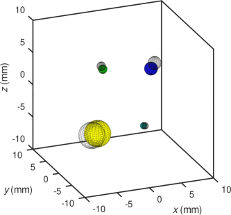
Figure 2: Initial arrangement of bubbles in the four-bubble cluster (the transparent spheres) and the position of the same bubbles after 2000 periods of oscillations of the driving ultrasound wave (coloured spheres).

It follows from this discussion that accounting for the translational motion of bubbles does not noticeably alter computational results. We also note that the spectral line positions and shapes corresponding to bubbles undergoing translational motion and interacting with their neighbours are almost identical to those of isolated non-interacting stationary gas bubbles (compare the colour-filled spectra with the spectra shown by the red lines in each panel in Fig. 1). This means that bubble translation does not affect their natural frequency within the considered computational time. In support of this conclusion, in Fig. 2 we compare the initial spatial bubble positions in the four-bubble cluster with the positions of the same bubbles after 2000 periods of the driving ultrasound wave. In agreement with the results of the analysis presented in Sec. III.2 we observe that bubble attraction is weak so that even after 2000 periods of oscillations the distance between them remains sufficiently large for the cluster to generate a usable AFC spectrum (and for the model to remain validity).

V Conclusions

We have proposed a new approach to the generation of spectrally-wide AFCs using oscillations of polydisperse gas bubble clusters in liquids. The plausibility of such an approach has been demonstrated via theoretical analysis and numerical simulation. In the model used in computations, we excite a bubble cluster with a low-pressure ultrasound wave at a frequency that is higher than the natural frequency of any bubble in the cluster. Bubbles within a cluster interact with each other and their acoustic spectra are affected by their neighbours. We choose the bubble sizes in such a way that their natural frequencies become integer multiples of the natural frequency of the largest bubble in the cluster. Because of that the spectra of individual bubbles contain multiple peaks, each of which can be unambiguously associated with the specific bubble within the cluster.

In agreement with the analysis and experimental observations reported in our previous publication [13], the interference of bubble responses at their natural frequencies with the driving ultrasound wave results in the amplitude modulation of the latter and in the appearance of equally-spaced sideband peaks in the spectrum. Moreover, the combination of sidebands and the ensemble of peaks originating directly from the oscillations at the natural bubble frequencies results in a quasi-continuum of equally spaced peaks. Its spectral composition depends on bubble radii and the frequency of a driving ultrasound wave. Therefore, it can be tuned by changing either of these parameters. In particular, because mm-sized gas bubbles are required to generate AFCs discussed in this work, a practical realisation of the proposed approach is technically straightforward. Indeed, a simple customised bubble generator consisting of a standard air pump and a diffuser made of a suitable porous material [13] would suffice to produce bubble clusters with the configuration investigated in this paper. We have also demonstrated that the attraction and potential coalescence of oscillating bubbles due to the action of the secondary Bjerknes force do not affect the generation of the AFC because coalescence occurs at a timescale that is much larger than the time needed for a reliable recording of AFC signals. Finally, our results are also expected to apply to smaller gas bubbles driven by ultrasound waves in high kHz and MHz frequency ranges, which paves the way for the generation of AFCs suitable for a wide range of technologically important applications.