Measurement and Modeling of Proton-Induced Reactions on
Arsenic from 35 to 200 MeV

Abstract

⁷²As is a promising positron emitter for diagnostic imaging that can be employed locally using a ⁷²Se generator. However, current reaction pathways to ⁷²Se have insufficient nuclear data for efficient production using regional 100–200 MeV high-intensity proton accelerators. In order to address this deficiency, stacked-target irradiations were performed at LBNL, LANL, and BNL to measure the production of the ⁷²Se/⁷²As PET generator system via ⁷⁵As(p,x) between 35 and 200 MeV. This work provides the most well-characterized excitation function for ⁷⁵As(p,4n)⁷²Se starting from threshold. Additional focus was given to report the first measurements of ⁷⁵As(p,x)⁶⁸Ge and bolster an already robust production capability for the highly valuable ⁶⁸Ge/⁶⁸Ga PET generator. Thick target yield comparisons with prior established formation routes to both generators are made. In total, high-energy proton-induced cross sections are reported for 55 measured residual products from ⁷⁵As, ${}^{\textnormal{nat}}$Cu, and ${}^{\textnormal{nat}}$Ti targets, where the latter two materials were present as monitor foils. These results were compared with literature data as well as the default theoretical calculations of the nuclear model codes TALYS, CoH, EMPIRE, and ALICE. Reaction modeling at these energies is typically unsatisfactory due to few prior published data and many interacting physics models. Therefore, a detailed assessment of the TALYS code was performed with simultaneous parameter adjustments applied according to a standardized procedure. Particular attention was paid to the formulation of the two-component exciton model in the transition between the compound and pre-equilibrium regions, with a linked investigation of level density models for nuclei off of stability and their impact on modeling predictive power. This paper merges experimental work and evaluation techniques for high-energy charged-particle isotope production in an extension to an earlier study of this kind.

I Introduction

Multi-hundred MeV proton accelerators are promising sites for the large scale production of medical radionuclides due to the high production rates enabled by their high-intensity beam capabilities and the long range of high-energy protons. However, the ability to reliably conduct isotope production at these accelerators and model relevant (p,x) reactions in the 100–200 MeV range is hampered by a lack of measured data.

In the effort to improve this state of proton-induced nuclear reaction data, irradiations of arsenic have been performed. The formation of ⁷²Se and ⁶⁸Ge from ⁷⁵As(p,x) is of particular interest for their application in diagnostic imaging as generators or “cows” for their decay daughters, ⁷²As and ⁶⁸Ga, respectively. The present general production data for ⁷²Se at incident proton energies in the 35–200 MeV range are scarce to non-existent. Low-energy ⁶⁸Ge production data have been thoroughly assessed and already contribute to a robust production capability set over the past decade, but extending knowledge for ⁶⁸Ge formation at higher-energies too should benefit its overall application. The 35–200 MeV range is especially relevant because it is characteristic of the Los Alamos Isotope Production Facility (IPF) and the Brookhaven LINAC Isotope Producer (BLIP), where medical isotopes are created for widespread use.

⁷²As ($t_{1/2}=26.0\ (1)$ h, 87.8 (22)% $\beta^{+}$ [1]) is a favourable positron emitting radionuclide for the imaging of slower biological processes. Its half-life makes ⁷²As-labelled radiopharmaceuticals useful for the observation of long-term metabolic processes, such as the enrichment and distribution of antibodies in tumour tissue, by positron emission tomography (PET) [2, 3]. ⁷²As offers the similar slow kinetic behaviour as the PET isotope ¹²⁴I ($t_{1/2}=4.1760\ (3)$ d, 22.7 (13)% $\beta^{+}$ [4]) but with a higher positron emission decay branch [5]. Furthermore, ⁷²As can form a promising pair with ⁷⁷As ($t_{1/2}=38.83\ (5)$ h, 100.0 (4)% $\beta^{-}$, 683.2 (17) keV $E_{\beta^{-},max}$ [6]) for combined imaging and radiotherapy [7, 8, 9]. The high sulfur affinity of arsenic, promoting its covalent binding to thiol groups, along with the toxicity of the ⁷⁷As decay spectrum, make ⁷²As/⁷⁷As an unique theranostic candidate [8, 10].

Current production methods for ⁷²As require a charged-particle beam in an accelerator setting. Existing accelerator pathways rely on ^natGe targets via the ^natGe(p/d,xn)⁷²As mechanisms in the 10–50 MeV incident particle energy range [3, 11]. However, these direct routes to ⁷²As constrain its use to medical centres nearby the production facility due to a half-life not appropriate for shipping or dispensing from a storage inventory. Additionally, direct production from ^natGe suffers from low thick target yields at these low incident energies and from co-production of the longer-lived radioisotopic impurities ^74,73,71As [3, 11]. Instead, recognition of the longer-lived ⁷²Se ($t_{1/2}=8.40\ (8)$ d [1]) as the parent precursor to ⁷²As creates the possibility for a ⁷²Se/⁷²As generator system [2, 11, 9]. Production of a generator results in ⁷²As free from other radioarsenic contaminants, on account of advantageous lifetime differences between ⁷²Se and neighboring Se nuclei, and availability restrictions at medical facilities across the globe. Measurements of a ^natBr(p,x)⁷²Se production route have been undertaken but the thick target yields, even approaching 200 MeV incident protons, are relatively low [3, 7, 12, 13]. Bromine targets subjected to high power may also pose heating and/or reactivity problems [12, 13]. The alternatively explored formation mechanism of ^nat/70Ge($\alpha$,xn)⁷²Se also suffers from low yields due to the short range of lower energy $\alpha$-particles combined with a relatively small ($<100$ mb) production peak [14].

In contrast, proton-induced reactions on arsenic offer a potentially improved production pathway to the ⁷²Se/⁷²As generator system. The combination of an expected sufficient cross section over a wide energy range with a naturally monoisotopic (⁷⁵As), stable material that can be appropriately formed into production targets makes high-intensity, high-energy proton irradiations an enticing approach.

⁶⁸Ga ($t_{1/2}=67.71\ (8)$ min, 88.91 (9)% $\beta^{+}$ [15]) has emerged as a significant short-lived positron emitter alongside the ubiquitous ¹⁸F for PET imaging in cases of general cancer, glioma, hypoxia, neuroendocrine tumours, and more [16, 17]. ⁶⁸Ga readily forms stable complexes with DOTA (a synthetically flexible metal chelating agent) and HBED, allowing peptides and other small molecules to be radiolabeled at high specific activities [18, 19]. NETSpot, using ⁶⁸Ga-DOTA, is an FDA approved PET imaging agent for neuroendocrine cancers [18]. Further, the compatibility of ⁶⁸Ga with a prostate-specific membrane antigen targeting ligand (PSMA-11 with HBED chelator) has led to a sought-after, highly successful PET tracer for the diagnosis of prostate cancer [16, 20, 18]. However, in a similar fashion to ⁷²As, direct production by typical ⁶⁵Cu($\alpha$,n)⁶⁸Ga and ⁶⁸Zn(p,n)⁶⁸Ga routes suffer from the same local accelerator production and shipping time constraints that inhibit widespread use [3]. Conversely, an indirect pathway to ⁶⁸Ga, through its long-lived ⁶⁸Ge ($t_{1/2}=270.93\ (13)$ d [15]) parent, constitutes an effective generator system more applicable for societal application.

While the elution and separation chemistry of the ⁶⁸Ge/⁶⁸Ga system has been extensively developed, nuclear data for ⁶⁸Ge production remains partially incomplete [17]. The ^natGa(p,xn)⁶⁸Ge route is the heavily studied, successful favourite of accelerator sites globally – particularly the prominent facilities of IPF, BLIP, and iThemba labs – but data only reaches up to 100 MeV. Other ⁶⁹Ga(p,xn)⁶⁸Ge, ^natGe(p,pxn)⁶⁸Ge, and ⁶⁶Zn($\alpha$,2n)⁶⁸Ge low-energy pathways have been explored but are less ideal due to excitation functions that peak in the 15–35 MeV range, which may be suboptimal for thick target yields, and present target manufacturing and purity concerns [17, 19]. Studying proton-induced reactions on arsenic gives a chance to strengthen the community’s total understanding of ⁶⁸Ge/⁶⁸Ga formation.

In this work, proton-induced nuclear reaction data for ⁷⁵As were measured for energies 35–200 MeV using the stacked-target method as part of the DOE Isotope Program’s Tri-laboratory Effort in Nuclear Data (TREND) between Lawrence Berkeley National Laboratory (LBNL), Los Alamos National Laboratory (LANL), and Brookhaven National Laboratory (BNL) [21]. We report the first cross section measurements for ⁷⁵As(p,x)⁶⁸Ge and the most well-characterized excitation function of ⁷⁵As(p,4n)⁷²Se to-date. Thick target yields are additionally calculated from the measured excitation functions and compared to established formation routes for the generator radionuclides to better inform accelerator facilities of optimal production parameters.

This stacked-target work has further provided 53 other high-energy (p,x) production cross section datasets for residual nuclei stemming from ⁷⁵As, ^natCu, and ^natTi targets.

These extensive measurements were also used to assess the predictions of multiple nuclear reaction codes. The standardized fitting procedure for reaction model parameters and pre-equilibrium adjustments developed in Fox et al. [21] was applied to the arsenic data, with an investigative focus to check if the proposed exciton model trends are seen.

In addition to studying pre-equilibrium, the fitting procedure provided insight into the appropriate level density models for a swath of nuclei. A discussion of the impact of level density knowledge on modeling predictive power is presented with a reflection of the limitations imposed on creating recommended high-energy charged-particle data.

The combination of experimental measurement and evaluation study presented in this work creates data with immediate application while contributing to an increasingly prioritized future need for high-energy modeling in the nuclear data community [22].

II Experimental Methods and Materials

This work is an outcome of the same set of experimental irradiations and activations performed for Fox et al. [21] but gives a focus to the analysis and interpretation of arsenic, titanium, and copper target foils not previously discussed. Charged-particle stacked-target irradiations were carried out at the 88-Inch Cyclotron at LBNL for proton energies of $E_{p}<55$ MeV, at IPF at LANL for $50<E_{p}<100$ MeV, and at BLIP at BNL for $100<E_{p}<200$ MeV.

The stacked-target technique is a typical methodology for charged-particle irradiations to simultaneously measure multiple high-fidelity energy-separated cross section values per reaction channel. A stacked-target includes thin foils of a target of interest in combination with thick degraders and monitor foils. The degraders selectively reduce the primary beam energy throughout the stack while the monitor foils can be used to characterize the evolving beam properties as it propagates through the targets. Detailed explanations of the technique can be read in [21, 23, 24, 25, 26, 27].

II.1 Stacked-Target Design

Individual stacks were created for each irradiation at each experimental site. The three stacks differed slightly in composition according to the physical constraints of each site’s irradiation geometry and as a function of expected residual radionuclide production based on beam current and energy parameters.

II.1.1 LBNL Stack and Irradiation

The 88-Inch Cyclotron stack consisted of 25 $\mathrm{\SIUnitSymbolMicro}$m ^natCu foils (99.95%, CU000420, Goodfellow Metals, Coraopolis, PA 15108-9302, USA) and thin metallic ⁷⁵As layers electroplated onto 10 $\mathrm{\SIUnitSymbolMicro}$m or 25 $\mathrm{\SIUnitSymbolMicro}$m ^natTi foil backings (99.6%, TI000213/TI000290, Goodfellow Metals).

Nine copper and titanium foils each were cut into 2.5 cm $\times$ 2.5 cm squares and characterized by taking four length and width measurements using a digital caliper (Mitutoyo America Corp.) and four thickness measurements taken at different locations using a digital micrometer (Mitutoyo America Corp.). Each foil was also massed multiple times using an analytical balance at 0.1 mg precision after being cleaned with isopropyl alcohol. The characterization of the approximately 2.25 cm diameter arsenic depositions onto titanium, pictured in Figure 1, was a more intensive process involving particle transmission and neutron activation analysis. These details and the description of the associated electroplating creation process are given in Voyles et al. [28], while the resulting thickness and areal density values can be seen in Table 1.

All targets were then sealed using DuPont Kapton polyimide film tape of either 43.2 $\mathrm{\SIUnitSymbolMicro}$m of silicone adhesive on 25.4 $\mathrm{\SIUnitSymbolMicro}$m of polyimide backing (total nominal 7.77 mg/cm²) or 43.2 $\mathrm{\SIUnitSymbolMicro}$m of silicone adhesive on 50.8 $\mathrm{\SIUnitSymbolMicro}$m of polyimide backing (total nominal 11.89 mg/cm²). The encapsulated foils were mounted to the center of hollow 5.7 cm $\times$ 5.7 cm aluminum frames. The frames protected the foils during handling and centered them in the beam pipe after the stack was fully arranged in the target box seen in Figure 2.

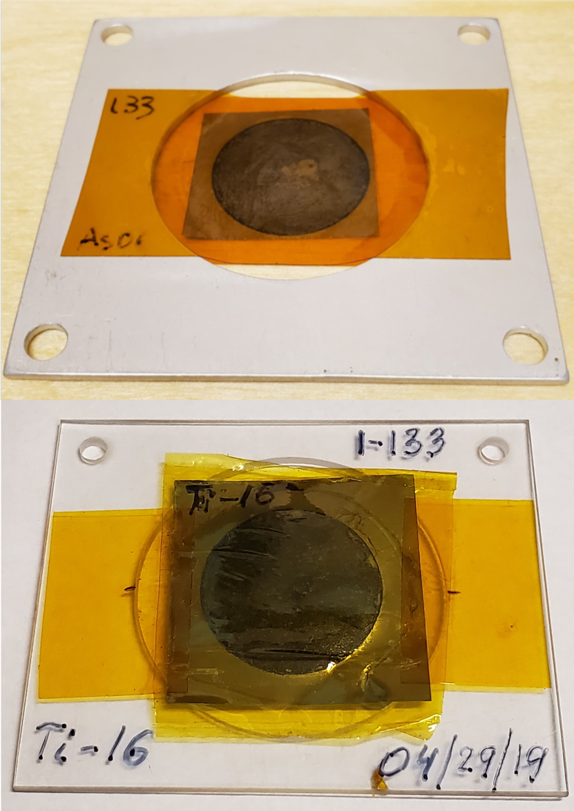
Figure 1: View of individual electroplated arsenic depositions on titanium backings within Kapton seals. The top target is sampled from the LBNL stack and is pictured after proton irradiation, where slight bubbling in the Kapton seal exists as a result of beam heating. The bottom target is part of the BNL stack prior to proton irradiation.

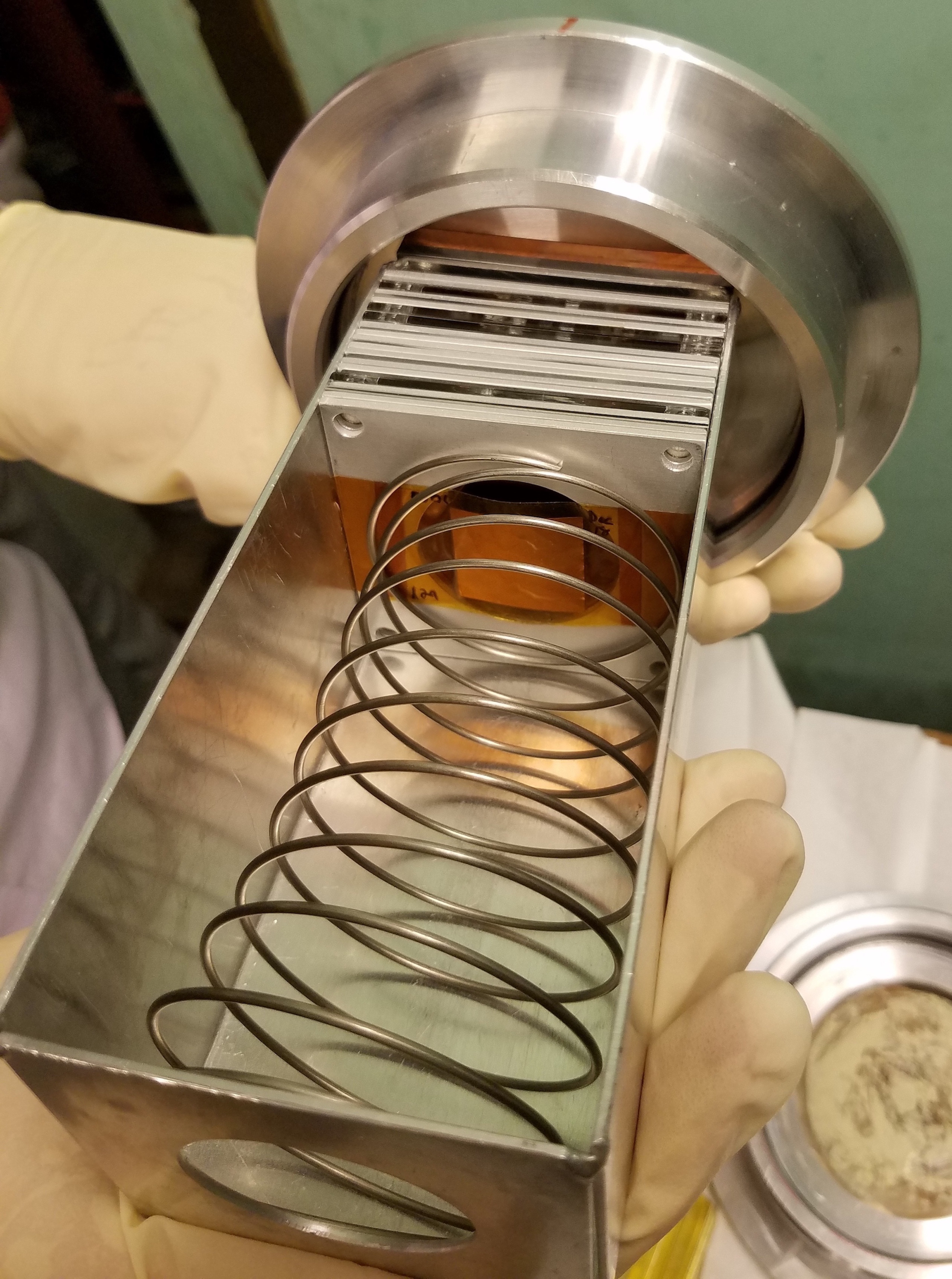
Figure 2: A top view of the assembled LBNL target stack prior to loading into the cyclotron beam pipe. The beam is first incident on the front facing copper target shown in the photo, as described in Table 1.

Multiple aluminum degraders were characterized in the same manner as the copper foils and included in the stack to yield nine different beam energy “compartments” for cross section measurements. One copper foil and one electroplated arsenic foil were placed into each of the nine compartments in the target box. Stainless steel plates (approximately 100 mg/cm²) were placed near the front and back of the stack for post-irradiation dose mapping using radiochromic film (Gafchromic EBT3) in order to examine the spatial profile of the beam entering and exiting the stack. The full detailed target stack ordering and properties for the LBNL irradiation are given in Table 1.

The stack was irradiated at the 88-Inch Cyclotron for 3884 seconds with a nominal 192 nA H⁺ beam. The total collected charge of the beam was measured using a current integrator connected to the electrically-isolated target holder, which was used to determine that the beam current was stable over the duration of the experiment. The mean beam energy extracted was 55.4 MeV with an approximately 1% uncertainty.

Table 1: Target stack design for irradiation at the 88-Inch Cyclotron. The proton beam initially hits the Cu-SN1 target and is subsequently transported through the rest of the shown stack order. The thickness and areal density measurements are prior to any application of the variance minimization techniques described in this work.

Target Layer	Thickness [$\mathrm{\SIUnitSymbolMicro}$m]	Areal Density [mg/cm2]	Areal Density Uncertainty [%]
Cu-SN1	24.81	22.23	0.33
As-SN1	3.24	1.85	9.8
Ti-SN1	25.00	11.265	1.0
SS Profile Monitor	130.0	100.12	0.07
Al Degrader E1	253.0	68.31	0.10
Al Degrader E2	252.7	68.24	0.10
Cu-SN2	24.88	22.29	0.08
As-SN2	1.69	0.97	9.9
Ti-SN2	25.00	11.265	1.0
Al Degrader D1	674.2	174.44	0.05
Cu-SN3	24.88	22.29	0.06
As-SN3	1.81	1.04	9.9
Ti-SN3	25.00	11.265	1.0
Al Degrader D2	664.5	174.87	0.06
Cu-SN4	24.87	22.28	0.04
As-SN4	2.22	1.27	10
Ti-SN4	25.00	11.265	1.0
Al Degrader E3	253.1	68.35	0.10
Cu-SN5	24.97	22.37	0.06
As-SN5	1.95	1.12	9.9
Ti-SN5	25.00	11.265	1.0
Al Degrader F1	181.5	46.91	0.12
Al Degrader F2	192.2	48.97	0.14
Cu-SN6	24.85	22.27	0.09
As-SN6	1.30	0.74	11
Ti-SN6	25.00	11.265	1.0
Al Degrader E4	252.9	68.29	0.10
Cu-SN7	24.67	22.11	0.39
As-SN7	2.36	1.35	8.9
Ti-SN7	10.00	4.506	1.0
Al Degrader C1	970.0	261.48	0.03
Cu-SN8	24.80	22.22	0.06
As-SN8	0.94	0.54	9.7
Ti-SN8	25.00	11.265	1.0
Al Degrader E5	252.7	68.24	0.10
Cu-SN9	24.90	22.31	0.10
As-SN9	0.57	0.32	10
Ti-SN9	25.00	11.265	1.0
SS Profile Monitor	130.0	100.48	0.07

II.1.2 LANL Stack and Irradiation

The LANL stack included copper, niobium, aluminum, and electroplated arsenic targets. The stack composition is described in detail in Fox et al. [21], where characterization procedures were very similar to the LBNL setup. A summary of the stack is provided in this paper in Table LABEL:LANLStack (see Appendix A). The stack was irradiated for 7203 seconds with an H⁺ beam of 100 nA nominal current. The beam current, measured using an inductive pickup, remained stable under these conditions for the duration of the irradiation. The mean beam energy extracted was 100.16 MeV with an approximately 0.1% uncertainty.

II.1.3 BNL Stack and Irradiation

The BNL stack was composed of copper, niobium, and electroplated arsenic targets. The exact specifications of the stack are given in Fox et al. [21] and a summary can be seen in Table 8 (see Appendix A). The stack was irradiated for 3609 seconds with an H⁺ beam of 200 nA nominal current. The beam current during operation was recorded using toroidal beam transformers and shown to remain stable under these conditions for the duration of the irradiation. The mean beam energy extracted was 200 MeV with an approximately 0.2% uncertainty [7].

II.2 Gamma Spectroscopy and Measurement of Foil Activities

II.2.1 LBNL

The gamma spectroscopy at the 88-Inch Cyclotron utilized an ORTEC GMX series (model GMX-50220-S) High-Purity Germanium (HPGe) detector and seven ORTEC IDM-200-VTM HPGe detectors. The GMX is a nitrogen-cooled coaxial n-type HPGe with a 0.5 mm beryllium window, and a 64.9 mm diameter, 57.8 mm long crystal. The IDMs are mechanically-cooled coaxial p-type HPGes with single, large-area 85 mm diameter $\times$ 30 mm length crystals and built-in spectroscopy electronics. The energy and absolute photopeak efficiency of the GMX and IDMs were calibrated using standard ¹³³Ba, ¹³⁷Cs, and ¹⁵²Eu sources. The efficiency model used in this work is the physical model presented by Gallagher and Cipolla [29].

Foil activity data was first collected from counts beginning approximately 45 minutes after the end-of-bombardment (EoB) and removal of the target stack from the beamline. The copper and electroplated arsenic foils were initially cycled through multiple 5–30 minute counts on the GMX during the 24 hours immediately following the irradiation. The counting distances from the GMX detector face were varied from 80 cm to 15 cm during this period subject to dead time constraints. Each electroplated arsenic foil was then transferred to an individual IDM detector where counts were collected in 1 hour intervals at a 10 cm distance from the IDM face over the next three weeks. The repeated counts of each foil helped to establish consistent decay curves for residual nuclides and reduce uncertainty in the spectroscopy analysis, particularly aiding in the determination of longer-lived products. Final 12–24 hour counts for the copper foils were captured on the GMX near the end of the three week period to record appropriate statistics for long-lived monitor channels.

The radiochromic film, developed by the stainless steel plates, showed that an $\approx$1 cm diameter proton beam was centered on the stack foils and properly inscribed within the size-limiting borders of the arsenic deposits throughout the stack.

II.2.2 LANL

The LANL experiment used a series of GEM and IDM HPGe detectors. The foil counting at LANL followed a similar cycling routine to LBNL, with counting times ranging from 10 minutes during the first hours after EoB to upwards of 8 hours over the course of 6 weeks after the irradiation for the stack’s 40 total targets. The LANL counting scheme is given explicitly in Fox et al. [21]. Notably, the electroplated arsenic targets of the LANL stack were shipped to LBNL in order to perform multi-week long counts with the LBNL GMX to better capture the ⁶⁸Ge signal, which remained weak in the longest of the LANL counts.

II.2.3 BNL

The BNL gamma spectroscopy setup incorporated two EURISYS MESURES 2 Fold Segmented “Clover” detectors in addition to one GMX and two GEM detectors. Foils were cycled in front of the many detectors for repeated short counts of 30 minutes or less during the first 24 hours after EoB. Data collection at BNL continued with multi-hour target counts for an additional day before the targets were shipped back to LBNL, arriving within two weeks after EoB. The LBNL GMX was used for multi-day to week-long counts of the copper, electroplated arsenic, and niobium foils over the course of the next 2+ months.

Further details of the BLIP activation and spectroscopy is provided in Fox et al. [21].

II.2.4 Activation Analysis

The UC Berkeley code package Curie [30] was used to analyze the collected gamma spectra from each irradiation. Decay curves for observed residual products were constructed from the count data with appropriate timing, efficiency, and attenuation corrections. EoB activities $A_{0}$ were then determined by fitting decay curves to the applicable Bateman equations [24, 21, 23]. A sample gamma-ray spectrum from an electroplated arsenic target is given in Figure 3.

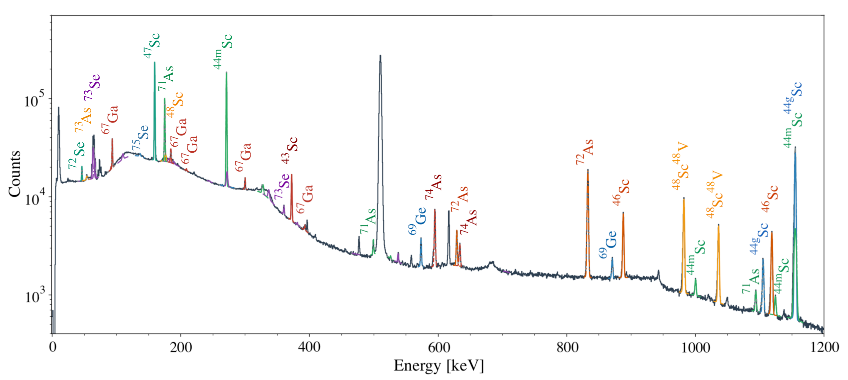
Figure 3: Example gamma-ray spectrum from the induced activation of an electroplated arsenic target in the LANL stack at approximately $E_{p}=91$ MeV. The spectrum was taken slightly beyond 2 days after EoB and the smooth fits to the peaks of interest shown are produced by the Curie package [31].

Independent, $(i)$, $A_{0}$ results were determined from decay curve fits where decay contributions from any precursors of a residual product could be distinguished or where no parent decay in-feeding existed. In cases where precursor contributions could not be distinguished, either due to timing or decay property limitations, cumulative, $(c)$, $A_{0}$ values for a residual product within a decay chain were instead calculated.

The total uncertainties in the determined EoB activities had contributions from fitted peak areas, evaluated half-lives and gamma intensities, regression parameters, and detector efficiency calibrations. Each contribution to the total uncertainty was assumed to be independent and was added in quadrature. The impact of calculated $A_{0}$ uncertainties on final cross section results is detailed in Section II.4.

II.3 Stack Current and Energy Properties

The proton beam energy and current at each target in a given stack was determined by monitor foil activation data, Curie’s Andersen & Ziegler-based Monte Carlo particle transport code, and a “variance minimization” approach, following the established methodology presented in Voyles et al. [23], Morrell et al. [24], Graves et al. [25].

The ^natTi(p,x)⁴⁸V, ⁴⁶Sc and ^natCu(p,x)^63,62Zn, ⁵⁸Co monitor reactions, taken from the IAEA-recommended data reference for charged-particle reactions [32], were used for the LBNL beam characterization. The results after variance minimization are shown in Figure 4 with plotted weighted averages of all the monitor reaction fluence predictions in each stack compartment. The weighted averages account for data and measurement correlations between the monitor reaction channels at each position in the stack and were used to create the uncertainty-weighted linear fit, also included in Figure 4 [33]. The fit is a global model applied due to the observed flat fluence depletion and provides an interpolation for the fluence and energy of each individual target of interest in the stack. This optimized linear model after variance minimization shows an approximately constant 207 nAh fluence throughout the LBNL stack.

Further details of the monitor foil calculations, variance minimization approach, and energy determinations for the LBNL experiment can be reviewed in Appendix B. An in-depth discussion of this same beam characterization procedure for the LANL and BNL stacks is provided in Fox et al. [21]. Recall that this work and Fox et al. [21] are outcomes of the same set of target stacks and irradiations meaning that the LANL and BNL fluence results and energy assignments from Fox et al. [21] are identically applied here.

The final deduced energy assignments, with associated uncertainties, for targets in all three stacks are provided in Tables 2, 3, and 4.

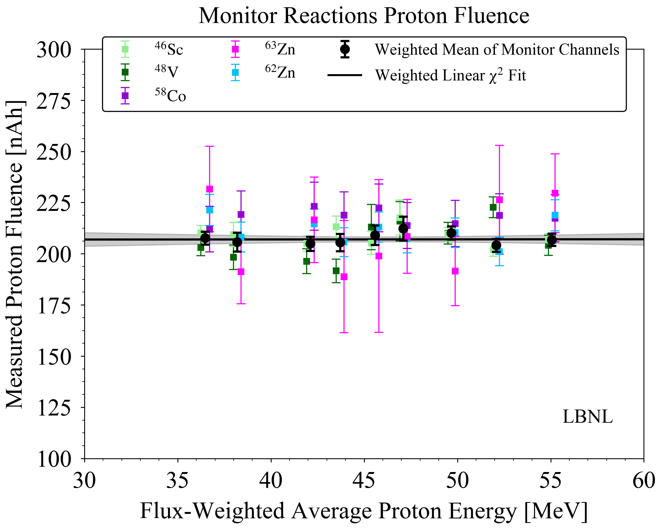
Figure 4: Plot of the proton beam fluence measured by monitor reactions in the LBNL stack following adjustments made by the variance minimization technique.

II.4 Cross Section Determination

Cross sections for observed products in this work were calculated from the typical activation formula,

$$\sigma=\frac{A_{0}}{I_{p}(\rho_{N}\Delta r)(1-e^{-\lambda t_{irr}})},$$ (1)

where $I_{p}$ is the beam current in protons per second at a given foil in a stack, $\rho_{N}\Delta r$ is the relevant foil’s areal number density, $\lambda$ is the decay constant for the observed residual product of interest, and $t_{irr}$ is the beam-on irradiation time.

Measured ⁷⁵As(p,x) cross sections are reported in Table 2 for ^75,73,72Se, ^74-70As, ^72,68-66Ga, ^69,68,66Ge, ${}^{69\textnormal{m},65}$Zn, and ^60,58-56Co.

^natCu(p,x) production cross sections for ^65,63,62Zn, ^64,61,60Cu, ^60,57-55Co, ⁵⁹Fe, ^57,56Ni, ^56,54,52Mn, ^51,49,48Cr, ⁴⁸V, and ${}^{47,46,44\textnormal{m}}$Sc are given in Table 3.

^natTi(p,x) experimental cross section results for ⁴⁸V, ${}^{48-46,44\textnormal{m},44\textnormal{g},43}$Sc, ⁴⁷Ca, ⁴⁴Ti, and ^43,42K are listed in Table 4.

In Tables 2 3, and 4, the cross sections for residual products are marked as either independent, $(i)$, or cumulative, $(c)$, referencing the distinction discussed in Section II.2.4 surrounding decay chains.

The final uncertainty contributions to the cross section measurements include uncertainties in evaluated decay constants (0.02–1.0%), foil areal density measurements (0.05–11%), proton current determination calculated from monitor fluence measurements and variance minimization (1.1–3.4%), and $A_{0}$ quantification that accounts for efficiency uncertainty in addition to other factors listed in Section II.2.4 (1.5–14%). These contributions were added in quadrature to give uncertainty in the final cross section results at the 3.5–17% level.

III Results and Discussion

The measured data from select reactions of particular interest to the medical applications community or for nuclear reaction modeling purposes are discussed in detail below. Plots of all other reported cross sections are given in Appendix C (Figures 21–69).

The experimentally extracted cross sections are compared with the predictions of nuclear reaction modeling codes TALYS-1.95 [34], CoH-3.5.3 [35], EMPIRE-3.2.3 [36], and ALICE-20 [37], each using default settings and parameters. A discussion of these default conditions and assumptions is provided in Fox et al. [21]. Comparisons with the TENDL-2019 library [38] are also made. Additionally, the cross section measurements in this work are compared to the existing body of literature data, retrieved from EXFOR [7, 39, 40, 41, 42, 43, 44, 45, 46, 47, 48, 49, 50, 51, 52, 53, 54, 55, 56, 57, 58, 59, 60, 61, 25, 23, 62, 63, 64, 65, 66, 67, 68, 24, 69, 70, 71, 72, 73, 74, 75, 76, 77, 78, 79].

Table 2: Summary of arsenic cross sections measured in this work. Subscripts $(i)$ and $(c)$ indicate independent and cumulative cross sections, respectively. Uncertainties are listed in the least significant digit, that is, 49.5 (14) MeV means 49.5 $\pm$ 1.4 MeV. Stack ID specifies which irradiation each measurement belongs to - Stack “BR” designates the Brookhaven irradiation, Stack “LA” designates the Los Alamos irradiation, and Stack “LB” designates the Lawrence Berkeley irradiation.

75As(p,x) Production Cross Sections [mb]
$E\mathrm{{}_{p}}$ [MeV]	192.28 (49)	177.01 (51)	163.21 (54)	148.55 (58)	133.75 (62)	119.66 (67)	104.09 (73)	91.09 (51)	79.19 (56)
Stack ID	BR	BR	BR	BR	BR	BR	BR	LA	LA
56Co(c)	0.823 (98)	0.337 (34)	0.581 (64)	0.436 (48)	0.169 (28)	-	-	-	-
57Co(c)	3.04 (46)	1.36 (18)	2.03 (28)	1.68 (25)	0.51 (17)	-	-	-	-
58Co(i)	3.62 (80)	-	2.81 (33)	2.25 (26)	0.84 (11)	0.32 (24)	0.07 (8)	-	-
60Co(i)	8.8 (11)	1.89 (20)	1.70 (20)	1.06 (14)	-	-	-	-	-
65Zn(c)	45.8 (77)	47.6 (58)	47.4 (63)	35.1 (43)	29.2 (38)	31.4 (38)	10.8 (15)	-	-
66Ga(c)	11.1 (66)	24.9 (66)	31 (17)	24.1 (98)	16.0 (42)	-	14.6 (39)	5.43 (89)	5.33 (95)
66Ge(c)	-	-	-	1.15 (49)	1.18 (22)	-	-	-	-
67Ga(c)	39.1 (46)	44.8 (45)	43.2 (47)	42.1 (43)	38.6 (49)	36.7 (36)	35.0 (39)	20.6 (19)	25.5 (24)
68Ga(i)	41.7 (83)	39.2 (62)	41.3 (58)	40.7 (69)	35.5 (53)	42.8 (55)	39.5 (52)	-	-
68Ge(c)	30.7 (46)	26.9 (30)	26.4 (32)	22.8 (27)	21.9 (30)	20.3 (23)	13.0 (16)	11.1 (22)	24.1 (41)
${}^{69\textnormal{m}}$Zn(i)	1.24 (19)	1.38 (22)	1.38 (17)	1.26 (14)	1.02 (24)	1.29 (13)	0.75 (13)	-	-
69Ge(c)	36.9 (43)	40.5 (43)	41.6 (50)	37.0 (42)	36.9 (49)	42.5 (44)	35.0 (39)	19.8 (20)	16.2 (16)
70As(c)	15.9 (18)	16.4 (17)	17.7 (19)	16.4 (17)	17.2 (21)	23.2 (23)	27.1 (28)	36.9 (39)	43.7 (45)
71As(c)	40.0 (45)	49.2 (51)	55.2 (64)	55.8 (60)	64.3 (79)	76.2 (76)	73.4 (75)	-	91.8 (85)
72Ga(c)	-	-	-	1.39 (57)	3.07 (95)	1.89 (68)	3.38 (82)	2.20 (29)	2.31 (49)
72As(i)	70.3 (77)	82.6 (82)	80.3 (90)	89.2 (94)	97 (12)	122 (12)	116 (12)	-	108.8 (99)
72Se(i)	6.12 (72)	6.90 (75)	8.12 (94)	8.09 (89)	8.4 (11)	11.2 (12)	11.6 (13)	-	15.2 (16)
73As(i)	95 (17)	125 (19)	138 (24)	128 (24)	138 (26)	166 (28)	172 (31)	180 (42)	174 (24)
73Se(c)	11.9 (15)	14.0 (16)	14.8 (17)	15.6 (18)	18.0 (24)	23.0 (25)	23.5 (27)	22.8 (29)	25.7 (35)
74As(i)	98 (11)	112 (12)	113 (16)	118 (14)	124 (18)	138 (14)	148 (18)	-	123 (12)
75Se(i)	5.55 (59)	6.65 (63)	7.47 (79)	6.80 (69)	7.44 (89)	9.23 (88)	9.48 (95)	6.08 (52)	10.10 (87)
$E\mathrm{{}_{p}}$ [MeV]	72.39 (60)	67.00 (64)	62.92 (67)	59.93 (69)	57.31 (72)	55.42 (74)	54.9 (13)	53.46 (76)	52.0 (14)
Stack ID	LA	LA	LA	LA	LA	LA	LB	LA	LB
66Ga(c)	2.88 (64)	-	-	-	-	-	-	-	-
67Ga(c)	16.4 (18)	6.2 (10)	2.32 (77)	1.00 (78)	0.91 (74)	-	-	-	-
68Ge(c)	41.4 (72)	39.2 (69)	31.1 (54)	14.1 (20)	-	-	-	-	-
69Ge(c)	17.6 (19)	20.6 (22)	25.6 (26)	34.5 (40)	39.4 (42)	37.4 (40)	41.5 (44)	39.6 (45)	35.8 (39)
70As(c)	33.1 (40)	-	2.3 (10)	-	-	-	-	2.3 (16)	-
71As(c)	131 (13)	143 (14)	130 (12)	128 (14)	103 (11)	74.9 (77)	63.9 (65)	53.6 (61)	32.3 (34)
72Ga(c)	1.72 (51)	2.25 (47)	-	1.26 (47)	-	1.31 (48)	-	1.03 (34)	-
72As(i)	146 (14)	169 (17)	188 (18)	238 (26)	262 (26)	249 (24)	277 (28)	266 (28)	246 (25)
72Se(i)	23.0 (25)	28.5 (31)	34.2 (36)	49.3 (58)	57.1 (62)	57.9 (62)	59.8 (63)	62.7 (71)	80 (12)
73As(i)	229 (32)	244 (35)	252 (35)	323 (47)	325 (47)	282 (40)	-	346 (60)	320 (53)
73Se(c)	37.4 (48)	39.0 (55)	45.2 (55)	54.2 (81)	62.1 (82)	57.0 (80)	60.1 (69)	65.4 (89)	65.4 (76)
74As(i)	153 (16)	158 (17)	157 (16)	186 (21)	185 (19)	169 (17)	188 (20)	170 (19)	182 (19)
75Se(i)	13.2 (12)	14.2 (13)	14.4 (13)	16.9 (18)	17.7 (17)	16.2 (15)	15.2 (16)	16.9 (18)	16.1 (18)
$E\mathrm{{}_{p}}$ [MeV]	51.44 (78)	49.5 (14)	47.0 (15)	45.4 (15)	43.6 (16)	41.9 (16)	38.0 (17)	36.3 (18)
Stack ID	LA	LB	LB	LB	LB	LB	LB	LB
69Ge(c)	40.6 (48)	31.5 (34)	27.6 (31)	17.6 (20)	13.0 (16)	12.0 (12)	-	-
71As(c)	39.6 (48)	17.4 (19)	9.7 (11)	6.44 (77)	8.2 (11)	3.46 (39)	-	-
72Ga(c)	-	-	-	-	-	-	0.21 (13)	-
72As(i)	280 (30)	226 (23)	219 (22)	207 (22)	-	131 (12)	73.8 (85)	41.9 (55)
72Se(i)	79.3 (92)	85 (14)	87 (13)	93 (10)	72.0 (85)	58.3 (73)	25.4 (40)	9.3 (14)
73As(i)	345 (52)	359 (65)	469 (79)	460 (69)	570 (100)	587 (85)	680 (110)	600 (94)
73Se(c)	80 (12)	69.6 (79)	91 (10)	92 (11)	114 (14)	205 (21)	235 (26)	307 (37)
74As(i)	186 (22)	181 (19)	194 (21)	193 (21)	-	234 (23)	218 (24)	239 (27)
75Se(i)	18.0 (19)	17.8 (20)	17.0 (18)	17.2 (20)	21.8 (35)	23.8 (23)	25.0 (31)	26.5 (39)

Table 3: Summary of copper cross sections measured in this work. Subscripts $(i)$ and $(c)$ indicate independent and cumulative cross sections, respectively. Uncertainties are listed in the least significant digit, that is, 90.94 (52) MeV means 90.94 $\pm$ 0.52 MeV. Stack ID specifies which irradiation each measurement belongs to - Stack “BR” designates the Brookhaven irradiation, Stack “LA” designates the Los Alamos irradiation, and Stack “LB” designates the Lawrence Berkeley irradiation.

natCu(p,x) Production Cross Sections [mb]
$E\mathrm{{}_{p}}$ [MeV]	192.54 (49)	177.28 (52)	163.49 (54)	148.86 (58)	134.08 (62)	120.02 (67)	104.49 (74)	90.94 (52)	79.03 (57)	72.22 (61)
Stack ID	BR	BR	BR	BR	BR	BR	BR	LA	LA	LA
44mSc(i)	0.289 (12)	0.1338 (63)	0.0784 (85)	0.0444 (40)	-	-	-	-	-	-
46Sc(i)	0.572 (21)	0.335 (11)	0.2381 (65)	0.1065 (59)	0.0616 (30)	0.0375 (24)	-	-	-	-
47Sc(c)	0.261 (46)	0.182 (31)	0.218 (26)	-	-	-	-	-	-	-
48V(c)	2.346 (84)	1.560 (47)	1.162 (30)	0.689 (29)	0.499 (15)	0.298 (45)	-	-	-	-
48Cr(c)	0.0707 (35)	0.0437 (19)	0.0263 (27)	0.0207 (11)	-	-	-	-	-	-
49Cr(c)	0.943 (67)	0.624 (60)	0.411 (46)	-	-	-	-	-	-	-
51Cr(c)	11.59 (42)	9.79 (29)	8.44 (21)	6.46 (26)	5.33 (13)	4.35 (13)	1.676 (68)	1.220 (61)	0.427 (49)	0.469 (43)
52Mn(c)	5.34 (19)	4.72 (14)	4.22 (11)	3.34 (12)	2.733 (70)	1.934 (59)	1.727 (70)	1.759 (67)	0.509 (22)	0.1008 (63)
54Mn(i)	16.26 (59)	15.72 (48)	14.88 (38)	13.4 (12)	12.48 (31)	11.05 (32)	7.30 (27)	6.63 (23)	3.87 (15)	3.86 (17)
55Co(c)	2.04 (11)	2.12 (11)	1.995 (97)	2.06 (10)	1.813 (91)	1.679 (90)	1.77 (10)	2.50 (18)	1.43 (11)	0.647 (60)
56Mn(c)	2.52 (15)	2.54 (15)	2.46 (14)	2.18 (13)	2.07 (13)	1.85 (11)	1.40 (10)	1.186 (57)	1.106 (54)	0.927 (43)
56Co(i)	12.50 (43)	12.65 (35)	12.57 (29)	13.18 (34)	12.29 (27)	11.55 (31)	10.51 (37)	10.31 (44)	12.12 (49)	12.68 (56)
56Ni(c)	0.072 (59)	0.089 (12)	0.116 (12)	0.105 (13)	0.131 (15)	0.093 (15)	-	0.0884 (75)	0.1103 (82)	0.1070 (81)
57Co(c)	43.0 (35)	42.3 (14)	43.1 (12)	43.6 (11)	44.5 (12)	44.7 (14)	42.2 (16)	44.7 (14)	37.7 (11)	36.9 (11)
57Ni(c)	1.687 (85)	1.787 (66)	1.820 (61)	1.776 (57)	-	-	-	1.76 (11)	1.286 (83)	1.391 (89)
59Fe(c)	1.180 (51)	1.209 (45)	1.189 (40)	1.100 (50)	1.097 (36)	1.045 (38)	0.923 (40)	0.931 (33)	0.867 (29)	0.817 (29)
60Co(i)	11.72 (47)	13.66 (61)	13.73 (48)	11.28 (55)	12.41 (35)	12.24 (38)	12.01 (48)	14.21 (42)	12.50 (37)	11.48 (36)
60Cu(c)	8.01 (42)	9.37 (48)	10.75 (57)	13.77 (77)	11.4 (10)	15.1 (14)	16.5 (19)	16.87 (75)	16.0 (10)	17.38 (90)
61Cu(c)	29.9 (16)	33.2 (16)	36.4 (17)	39.0 (17)	42.9 (19)	46.6 (22)	55.7 (29)	60.6 (30)	54.3 (29)	72.5 (35)
62Zn(i)	1.71 (11)	2.16 (13)	1.86 (12)	2.44 (14)	2.39 (15)	3.42 (19)	3.26 (21)	-	-	-
63Zn(i)	3.52 (34)	4.32 (45)	5.25 (63)	6.05 (87)	5.52 (97)	5.73 (93)	-	8.40 (52)	10.90 (71)	12.98 (78)
64Cu(i)	26.3 (15)	31.7 (18)	30.8 (34)	35.1 (18)	36.6 (35)	40.7 (22)	44.7 (39)	52.0 (57)	40.4 (55)	50.3 (51)
65Zn(i)	1.13 (26)	1.52 (20)	1.61 (16)	1.53 (11)	1.938 (83)	2.200 (78)	2.69 (11)	2.868 (95)	3.257 (95)	3.68 (11)
$E\mathrm{{}_{p}}$ [MeV]	66.81 (65)	62.73 (68)	59.73 (71)	57.11 (73)	55.21 (75)	55.2 (13)	53.24 (77)	52.2 (14)	51.22 (80)	49.9 (14)
Stack ID	LA	LA	LA	LA	LA	LB	LA	LB	LA	LB
51Cr(c)	0.512 (37)	0.409 (38)	0.328 (33)	0.278 (29)	-	-	-	-	-	-
54Mn(i)	4.70 (17)	4.95 (33)	4.70 (27)	4.10 (20)	3.41 (15)	3.58 (14)	2.65 (11)	2.31 (13)	1.848 (74)	1.25 (10)
55Co(c)	0.169 (22)	0.077 (15)	0.060 (20)	0.043 (12)	0.0394 (92)	0.0127 (40)	-	-	0.0162 (69)	-
56Mn(c)	0.644 (33)	0.460 (25)	0.243 (18)	0.171 (15)	0.161 (14)	0.101 (13)	0.089 (11)	-	0.0541 (91)	-
56Co(i)	10.95 (46)	7.66 (32)	4.47 (18)	2.405 (99)	1.272 (62)	-	0.713 (39)	-	0.373 (57)	-
56Ni(c)	0.0837 (61)	0.0518 (37)	0.0330 (28)	0.0144 (28)	0.0082 (26)	-	0.0076 (22)	-	0.0043 (13)	-
57Co(c)	42.4 (13)	50.0 (21)	55.9 (23)	59.5 (26)	58.7 (26)	64.6 (50)	58.0 (25)	55.6 (12)	54.8 (24)	49.9 (10)
57Ni(c)	1.78 (11)	2.32 (10)	2.61 (12)	2.73 (12)	2.60 (12)	2.608 (99)	2.38 (11)	1.942 (62)	1.985 (90)	1.502 (47)
59Fe(c)	0.775 (27)	0.690 (29)	0.618 (26)	0.516 (22)	0.419 (19)	-	0.322 (14)	-	0.227 (10)	-
60Co(i)	11.68 (36)	12.22 (49)	12.15 (47)	11.60 (46)	10.88 (51)	10.34 (41)	10.77 (49)	10.04 (39)	10.28 (40)	9.53 (36)
60Cu(c)	18.6 (15)	27.2 (23)	-	26.1 (38)	26.4 (29)	30.1 (27)	-	33.6 (25)	-	29.5 (25)
61Cu(c)	82.8 (39)	89.7 (42)	-	91.9 (44)	94.2 (45)	91.1 (42)	93.6 (45)	94.0 (42)	97.5 (47)	103.7 (45)
63Zn(i)	12.29 (88)	14.0 (11)	16.3 (13)	17.5 (16)	17.9 (20)	-	-	-	-	-
64Cu(i)	61.7 (60)	51.4 (56)	63.0 (62)	66.6 (66)	59.7 (56)	60.7 (30)	55.4 (59)	56.1 (28)	62.7 (62)	57.3 (32)
65Zn(i)	4.05 (11)	4.21 (20)	4.39 (19)	4.66 (21)	4.79 (24)	4.53 (23)	5.32 (28)	4.65 (25)	5.30 (26)	5.51 (28)
$E\mathrm{{}_{p}}$ [MeV]	47.3 (15)	45.8 (15)	43.9 (16)	42.3 (16)	38.4 (17)	36.7 (18)
Stack ID	LB	LB	LB	LB	LB	LB
54Mn(i)	0.533 (15)	0.160 (43)	0.091 (29)	0.020 (18)	0.076 (30)	0.092 (28)
57Co(c)	36.36 (68)	29.27 (61)	17.91 (41)	11.09 (29)	1.446 (96)	0.398 (34)
57Ni(c)	0.909 (32)	0.634 (26)	0.309 (19)	0.1257 (93)	-	-
60Co(i)	8.78 (16)	7.72 (31)	7.12 (31)	5.95 (32)	4.95 (27)	4.35 (24)
60Cu(c)	19.3 (22)	9.3 (21)	5.5 (17)	4.7 (18)	-	-
61Cu(c)	112.6 (48)	125.9 (54)	137.7 (59)	156.9 (67)	179.8 (77)	187.4 (82)
64Cu(i)	58.1 (31)	66.5 (33)	59.7 (30)	64.9 (31)	63.1 (33)	74.4 (36)
65Zn(i)	5.57 (12)	5.50 (26)	6.19 (27)	6.32 (29)	6.97 (30)	7.33 (34)

Table 4: Summary of titanium cross sections measured in this work. Subscripts $(i)$ and $(c)$ indicate independent and cumulative cross sections, respectively. Uncertainties are listed in the least significant digit, that is, 72.34 (61) MeV means 72.34 $\pm$ 0.61 MeV. Stack ID specifies which irradiation each measurement belongs to - Stack “BR” designates the Brookhaven irradiation, Stack “LA” designates the Los Alamos irradiation, and Stack “LB” designates the Lawrence Berkeley irradiation.

natTi(p,x) Production Cross Sections [mb]
$E\mathrm{{}_{p}}$ [MeV]	192.26 (49)	176.99 (51)	163.18 (54)	148.52 (58)	133.72 (62)	119.63 (67)	104.05 (74)	91.05 (51)	79.15 (57)
Stack ID	BR	BR	BR	BR	BR	BR	BR	LA	LA
42K(i)	7.54 (78)	6.45 (70)	6.83 (66)	6.34 (67)	6.92 (64)	5.56 (62)	6.10 (88)	6.73 (47)	6.48 (43)
43K(c)	2.62 (10)	2.493 (90)	2.84 (11)	2.34 (10)	2.23 (10)	2.116 (83)	1.95 (13)	1.830 (58)	1.349 (45)
43Sc(c)	16.5 (11)	15.9 (11)	12.8 (22)	15.17 (95)	17.1 (11)	20.0 (14)	-	22.8 (19)	15.0 (16)
${}^{44\textnormal{g}}$Sc(i)	25.1 (13)	26.5 (16)	27.9 (13)	28.49 (97)	28.5 (10)	31.5 (17)	31.7 (15)	32.2 (19)	39.3 (22)
${}^{44\textnormal{m}}$Sc(i)	11.46 (44)	11.88 (40)	12.71 (37)	13.43 (39)	14.47 (80)	14.82 (85)	19.1 (16)	21.34 (72)	22.29 (73)
44Ti(c)	2.7 (18)	2.8 (11)	3.3 (10)	4.37 (42)	3.3 (17)	4.55 (49)	-	-	-
46Sc(i)	34.0 (13)	36.1 (12)	38.2 (11)	39.3 (10)	39.3 (11)	40.9 (13)	41.5 (16)	42.1 (15)	42.3 (13)
47Ca(c)	0.167 (22)	0.187 (27)	0.168 (30)	0.158 (39)	-	-	-	-	-
47Sc(i)	25.7 (21)	25.84 (98)	26.53 (87)	26.82 (84)	26.2 (13)	26.70 (97)	26.0 (28)	23.5 (12)	22.4 (11)
48Sc(i)	2.31 (15)	2.35 (16)	1.85 (44)	1.88 (13)	2.53 (31)	-	2.65 (42)	2.45 (13)	2.35 (13)
48V(i)	3.62 (13)	4.11 (13)	4.16 (12)	4.86 (12)	5.60 (17)	6.24 (20)	7.06 (28)	-	-
$E\mathrm{{}_{p}}$ [MeV]	72.34 (61)	66.95 (64)	62.87 (67)	59.88 (70)	57.26 (72)	55.36 (74)	54.9 (13)	53.40 (76)	51.9 (14)
Stack ID	LA	LA	LA	LA	LA	LA	LB	LA	LB
42K(i)	6.94 (49)	7.32 (51)	6.57 (43)	5.62 (37)	4.30 (31)	3.23 (23)	2.86 (20)	2.77 (22)	1.72 (11)
43K(c)	1.295 (46)	1.358 (44)	1.339 (45)	1.425 (48)	1.408 (48)	1.532 (51)	1.400 (34)	1.439 (54)	1.333 (28)
43Sc(c)	15.4 (14)	13.9 (15)	15.2 (14)	15.7 (17)	17.9 (17)	18.6 (20)	14.22 (84)	19.0 (17)	15.83 (88)
${}^{44\textnormal{g}}$Sc(i)	35.4 (23)	-	30.4 (17)	27.7 (17)	21.3 (27)	24.65 (78)	21.3 (12)	22.22 (71)	22.2 (12)
${}^{44\textnormal{m}}$Sc(i)	23.03 (78)	21.13 (69)	18.18 (61)	15.97 (53)	14.23 (47)	13.52 (45)	12.02 (24)	12.79 (42)	10.48 (22)
46Sc(i)	44.8 (16)	48.0 (16)	50.0 (17)	51.8 (21)	53.2 (19)	55.5 (21)	-	55.3 (18)	-
47Sc(i)	23.2 (11)	23.7 (11)	23.8 (11)	23.9 (11)	23.6 (11)	23.5 (11)	20.82 (65)	22.7 (11)	19.08 (64)
48Sc(i)	2.33 (12)	2.30 (12)	2.28 (13)	2.18 (15)	2.131 (87)	2.02 (13)	1.649 (85)	2.01 (12)	1.596 (44)
$E\mathrm{{}_{p}}$ [MeV]	51.39 (79)	49.5 (14)	46.9 (15)	45.4 (15)	43.5 (16)	41.9 (16)	38.0 (17)	36.2 (18)
Stack ID	LA	LB	LB	LB	LB	LB	LB	LB
42K(i)	1.67 (16)	1.151 (90)	0.786 (67)	0.670 (80)	0.571 (55)	-	0.378 (45)	-
43K(c)	1.394 (52)	1.169 (25)	0.863 (19)	0.645 (17)	0.473 (12)	-	0.1122 (65)	-
43Sc(c)	20.6 (22)	16.12 (90)	16.32 (91)	15.80 (92)	-	13.18 (85)	9.38 (58)	6.54 (42)
${}^{44\textnormal{g}}$Sc(i)	23.24 (72)	19.4 (12)	22.7 (15)	22.3 (16)	23.8 (17)	25.1 (11)	29.8 (11)	33.73 (97)
${}^{44\textnormal{m}}$Sc(i)	12.86 (42)	11.54 (26)	12.00 (28)	11.61 (22)	12.16 (28)	12.24 (26)	15.03 (39)	13.45 (32)
46Sc(i)	59.7 (21)	-	-	-	-	-	-	-
47Sc(i)	23.0 (11)	20.41 (87)	20.89 (92)	19.87 (50)	20.37 (72)	19.16 (57)	23.62 (93)	22.35 (70)
48Sc(i)	2.01 (12)	1.836 (70)	1.809 (51)	1.684 (91)	1.627 (49)	1.370 (52)	1.296 (62)	1.003 (70)

III.1 ⁷⁵As(p,4n)⁷²Se Cross Section

⁷²Se decays 100% by electron capture to the first 1⁺ excited state in ⁷²As. This leaves a 45.89 keV ($I_{\gamma}=57.2\ (4)$%) $\gamma$-ray as the only direct detectable signature of ⁷²Se formation from the HPGe equipment used in this work. However, ⁷²Se production could additionally be quantified using the ⁷²As decay gamma-rays after ⁷²Se/⁷²As were in secular equilibrium at least 11 days after EoB. The results from each measurement method were seen to be very comparable but only the secular equilibrium values were recorded, and plotted in Figure 5, due to comparatively reduced uncertainties.

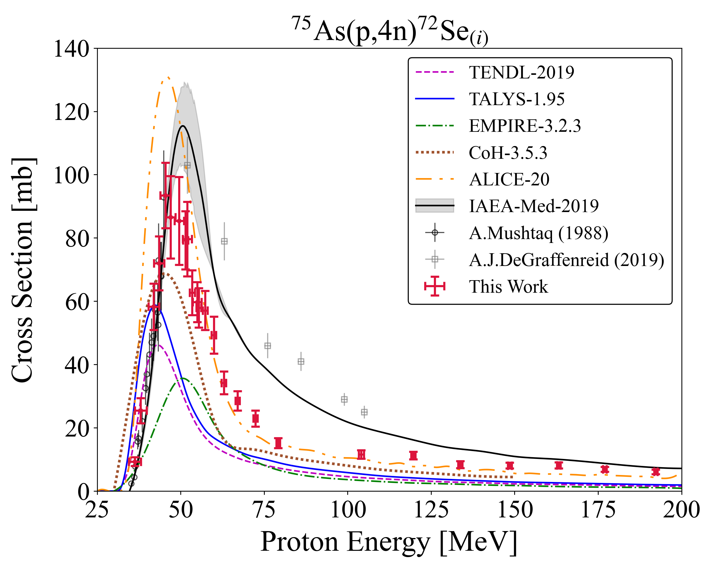
Figure 5: Experimental and theoretical cross sections for ⁷²Se production, peaking near 90 mb around 50 MeV.

Only two prior experimental datasets partially measured this excitation function. The Mushtaq et al. [39] results cover the low energy production from threshold towards the maximum of the compound peak near 50 MeV and agree well with the measurements of this work. The second prior experimental dataset from DeGraffenreid et al. [7] covers a broader higher-energy portion of the excitation function between 52–105 MeV. A large discrepancy exists between the DeGraffenreid et al. [7] data and the values reported here. This difference is most evident for the cross section above 60 MeV where our measurements demonstrate a much more constrained “bell-shape” for the compound peak with a pre-equilibrium “tail” that decreases in magnitude quicker than expressed by DeGraffenreid et al. [7]. These differences are possibly partly a function of the contrasting experimental methodologies between this work and DeGraffenreid et al. [7]. DeGraffenreid et al. [7] did not use a stacked-target technique, but instead used multiple irradiations with thicker GaAs wafer targets, a much larger beam current, and analysis by chemical dissolution of the targets with subsequent radioassays on an HPGe using solution aliquots.

The TALYS, CoH, and ALICE reaction codes, along with the TENDL evaluation, demonstrate a similar shape though all but ALICE underpredict the compound peak cross section magnitude. Incorrect compound peak energy centroids are a pervasive error among all the calculations for this channel, generally as a function of the codes’ poor threshold predictions. TENDL perhaps best matches the experimental threshold and rising edge behaviour of the excitation function but its incorrect magnitude, on account of misestimated competition with adjacent channels, muddles some of the comparison of the evaluation to the data.

In general, the variation in peak centroid location between the codes is typical and is a function of the differing pre-equilibrium calculations. Small differences between pre-equilibrium models in the codes can amplify the impact caused by particles emitted in pre-equilibrium that carry a significant amount of energy, which ultimately alter which compound nucleus is formed at a given incident energy [24]. Consequently, the improper pre-equilibrium tail modeling among TALYS, CoH, EMPIRE, and TENDL is noteworthy because it is an error that will propagate to the thresholding and rising edge behaviour in residual products that are energetically downstream of this (p,4n) channel.

Moreover, EMPIRE performs worst among the codes likely on account of these incorrect pre-equilibrium results for residual products closer in mass to the target nucleus. In this ⁷²Se channel, the errors in EMPIRE manifest as an estimated rising edge with a much too small of a slope and the largest magnitude underprediction.

The production cross section of ⁷²Se has also been evaluated as part of an IAEA coordinated research project (IAEA-Med-2019) focused on the recommendation of data for medical radionuclides, and in specific, diagnostic positron emitters [3]. The DeGraffenreid et al. [7] data were not avaialble at the time of the IAEA evaluation and though the IAEA prediction reaches a similar peak to DeGraffenreid et al. [7], which is above the peak predicted in this work, the IAEA recommendation does not support the very broad compound peak.

It is worth reflecting that these ⁷²Se production results, i.e., the proper characterization of an excitation function from threshold to 200 MeV where little prior data existed, are emblematic of the overall TREND endeavour.

III.2 ⁷⁵As(p,x)⁶⁸Ge Cross Section

The results reported here represent the first measurement of this channel. The ⁶⁸Ge production cross section proved difficult to quantify in this work due to its long half-life ($t_{1/2}=270.93\ (13)$ d [15]) and the lack of gamma-ray emissions. ⁶⁸Ge decays 100% by electron capture directly to the ground state of ⁶⁸Ga. As a result, it was necessary to rely on the still weak, but strongest available, 1077.34 keV ($I_{\gamma}=3.22\ (3)$%) $\gamma$-ray from the decay of ⁶⁸Ga to measure the ⁶⁸Ge formation cross section [80]. ⁶⁸Ga is short-lived with a 67.71 (8) min half-life and it quickly falls into secular equilibrium with ⁶⁸Ge [15]. Therefore, all 1077.34 keV emissions measured in the arsenic target spectra taken months after the irradiation dates were solely attributable to the decay of the initial cumulative ⁶⁸Ge population. Multi-week-long counts were required to achieve reasonable statistics for the 1077.34 keV signal.

The ensuing measured ⁷⁵As(p,x)⁶⁸Ge excitation function is given in Figure 6. No cross sections were extracted from the LBNL irradiation or the rear-end of the LANL stack as the incident proton energies were below or too near threshold for measurable ⁶⁸Ge production. The given excitation function in Figure 6 is the first measurement of ⁶⁸Ge formation from arsenic up to 200 MeV. The excitation function shows a peak of approximately 42 mb at 72 MeV due to the ⁷⁵As(p,$\alpha$4n)⁶⁸Ge pathway and a high-energy increasing pre-equilibrium tail from formation mechanisms where $\alpha$-particle emission is replaced by 2p2n. The cross section is additionally impacted by the shape of the ⁶⁸As excitation function since the given result is cumulative.

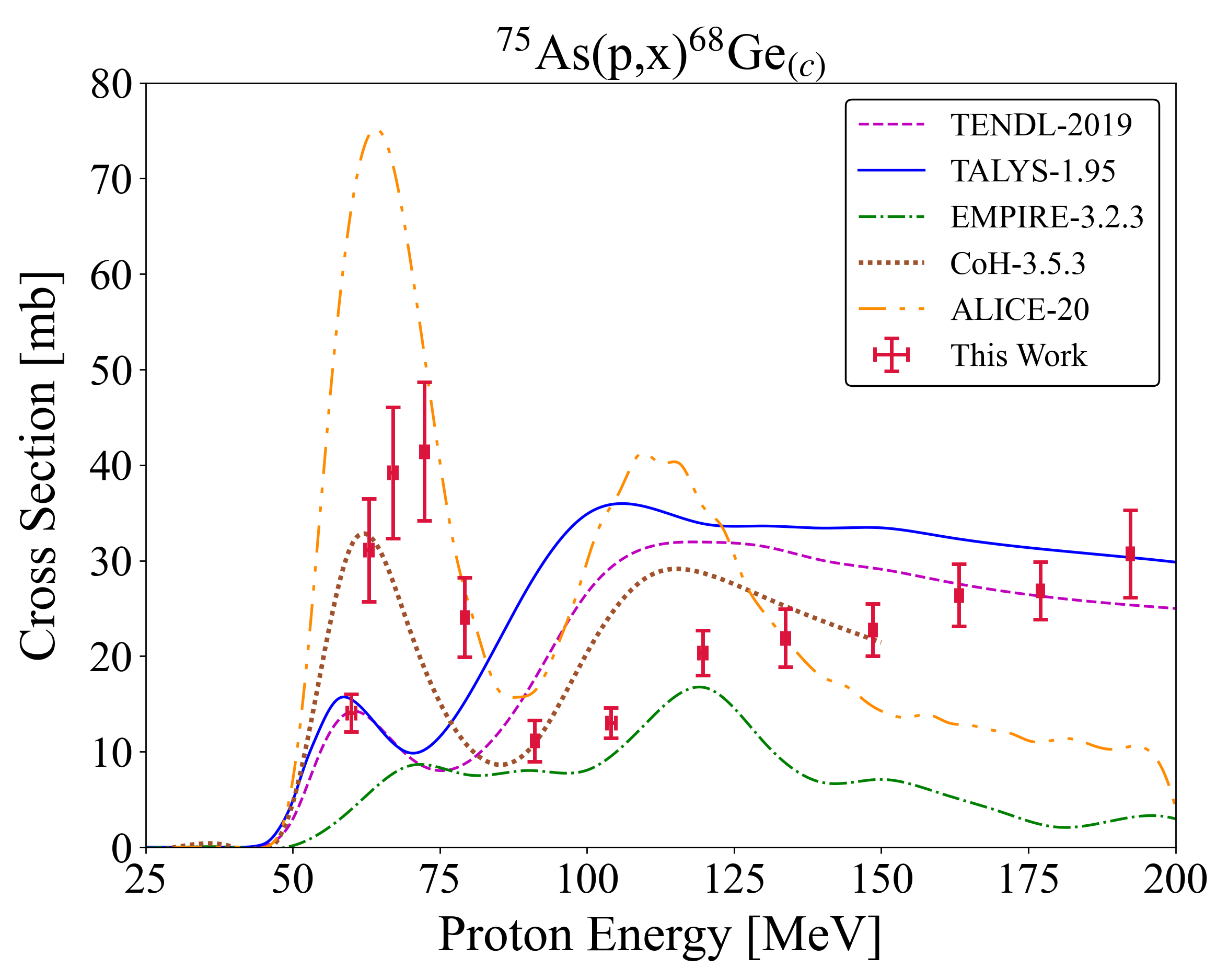
Figure 6: Experimental and theoretical cross sections for ⁶⁸Ge production, peaking near 42 mb around 72 MeV.

Interestingly, EMPIRE’s overprediction of the compound peak energy centroid for ⁷²Se production versus all other codes (Figure 5) is also seen for the ⁶⁸Ge excitation function except it is a fairly accurate representation of reality in Figure 6. However, this energy comparison is the endpoint of EMPIRE’s accuracy as its excitation function shape and magnitude are markedly incorrect.

ALICE continues to overestimate the compound peak magnitude and it even incorrectly predicts a higher-energy second compound peak rather than a pre-equilibrium tail. CoH performs similarly to ALICE but at a more correct magnitude albeit at a shifted centroid energy of near 10 MeV below the experimental data. Both TALYS and TENDL correctly demonstrate a significant pre-equilibrium tail with an approximately correct shape, similar to CoH, but the relative magnitudes between their peaks and tails are erroneous.

It is important to temper expectations for the predictive power of these codes in calculating the ⁶⁸Ge production seen here since this is a cumulative result. Note that in the cumulative cases of this work, the code calculations shown include necessary summing of decay precursor contributions. ⁶⁸Ge therefore requires calculation contributions from three residual products and ultimately only makes up a minor $\approx$5% of the total non-elastic cross section, which creates a difficult predictive case.

III.3 ⁷⁵As(p,3n)⁷³Se Cross Section

The ⁷⁵As(p,3n)⁷³Se excitation function is the most well-characterized residual product channel in the prior literature data. The measured cross sections extracted from the LBNL and LANL irradiations are shown in Figure 7 to agree very well with these existing results. Note that the reported cross sections are cumulative and include the formation contribution from the short-lived parent isomer ${}^{\textnormal{73m}}$Se ($t_{1/2}=39.8\ (13)$ min) in addition to the longer-lived ($t_{1/2}=7.15\ (8)$ h) ground state [81]. The results of the BNL irradiation help to extend the excitation function and characterize its tail behaviour up to 200 MeV. The consistency between our results and the literature data compiled in EXFOR builds confidence in the energy and current assignments determined in this work as well as the overall measurement and data analysis methodology.

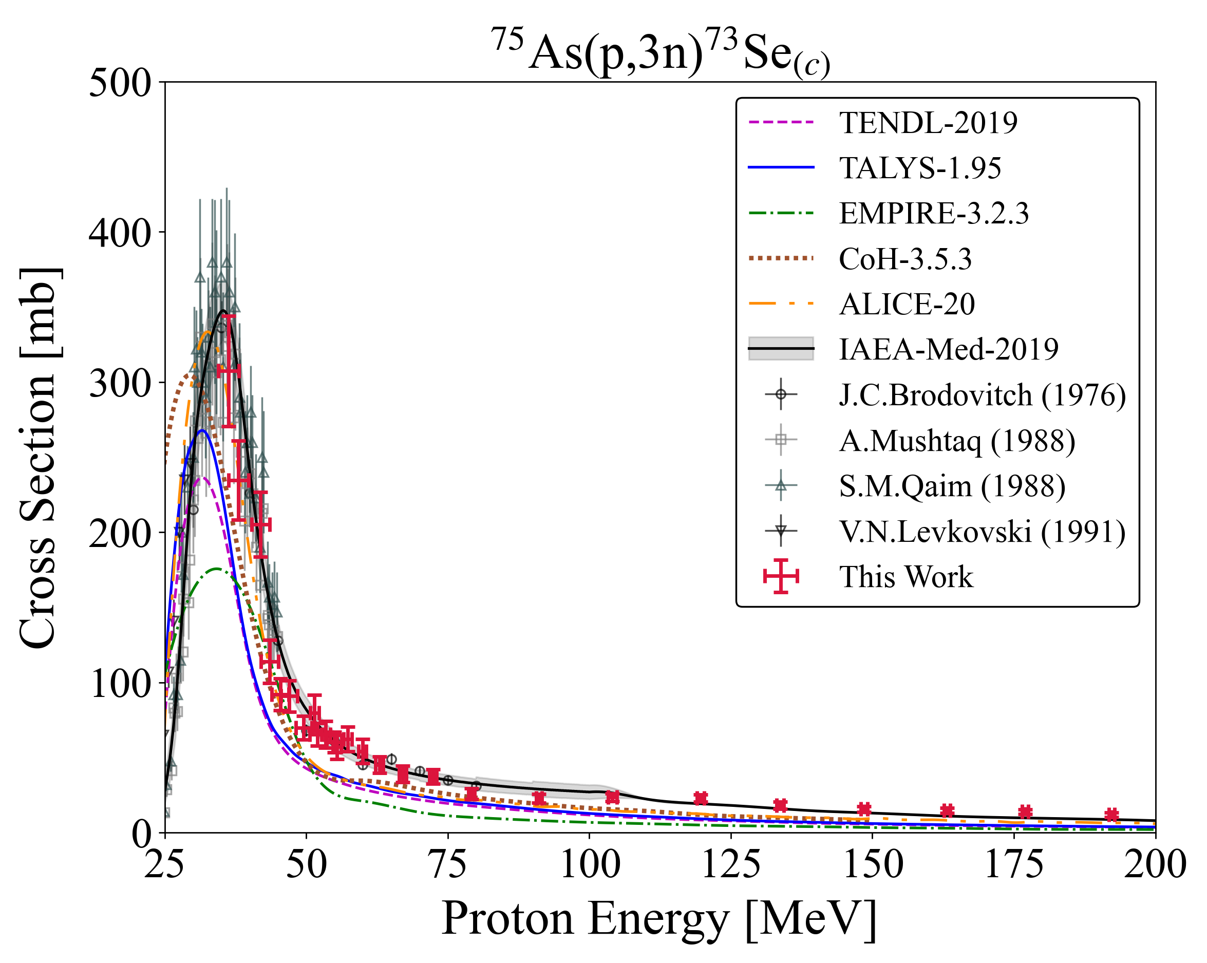
Figure 7: Experimental and theoretical cross sections for ⁷³Se production, peaking near 330 mb around 35 MeV.

The default TALYS and EMPIRE predictions both underestimate the compound peak magnitude, EMPIRE decidedly more so than TALYS, while TALYS also shifts the peak energy lower than experimentally observed. The ALICE calculation performs best here with an appropriate peak magnitude and nearly proper tail shape, which is just incorrectly shifted similar to TALYS. TENDL replicates TALYS very closely other than a slightly reduced peak magnitude. CoH significantly mispredicts the channel’s rising edge resulting in a more severe energy shift than both TALYS and ALICE.

The measured falling edge of the compound peak is additionally relevant to the medical community as ⁷⁵As(p,3n) has been shown as the most advantageous route to the nonstandard positron emitter ⁷³Se [82]. In this vein, the production of ⁷³Se has also been evaluated by the IAEA and this recommended fit is given in Figure 7 [3]. The IAEA fit is seen to agree very well with the measured data in this paper.

It is worth noting that although the cross section averages only $\approx$40 mb from 50–200 MeV, the greater range of incident protons at 200 MeV as compared to 50 MeV would lead to a more than doubling in the overall ⁷³Se production yield. This brief consideration is representative of the value inherent to high-current, high-energy proton accelerator facilities and rationalizes the effort to measure high-energy reaction data for potential production targets such as arsenic.

III.4 ⁷⁵As(p,p3n)⁷²As Cross Section

The direct measurement of ⁷²Se decay allowed for the subsequent independent cross section quantification of ⁷²As. The cross section results are presented in Figure 8 and are the measured first data for this reaction channel.

The modeling predictions all perform similarly in this channel, in contrast to the large variations seen for nearby ⁷²Se and ⁷³Se production. EMPIRE, CoH, and ALICE underpredict the high-energy pre-equilibrium tail for ⁷²As relative to TALYS and TENDL, though the former trio of codes have the better energy placement of the compound peak centroid.

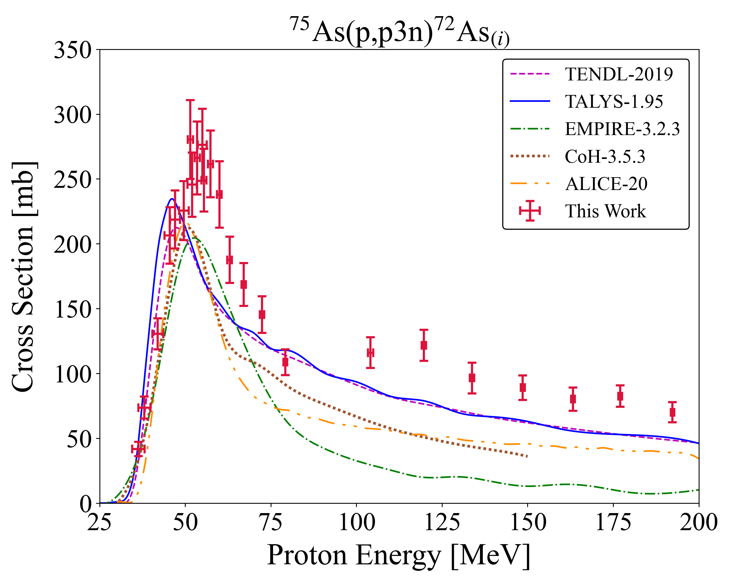
Figure 8: Experimental and theoretical cross sections for ⁷²As production, peaking near 275 mb around 55 MeV.

III.5 ^natTi(p,x)^44m/gSc Cross Section

The production of ^44gSc ($t_{1/2}=3.97\ (4)$ h [83]) is of general interest as an emerging radiometal for nuclear imaging and theranostic purposes [3, 84, 85, 82]. While the measurements of the ^natTi(p,x)^44m/gSc excitation functions extracted from the titanium monitor foils included in the target stacks may not give an ideal production route for this medical application, these cross section results do give the only observable isomer and ground state pair from the three irradiations. As a result, this work provides a large update to the ^44mSc ($t_{1/2}=58.61\ (10)$ h, $J^{\pi}=6^{+}$) to ^44gSc ($t_{1/2}=3.97\ (4)$ h, $J^{\pi}=2^{+}$) [83] isomer-to-ground state ratio via ^natTi(p,x), as seen in Figure 9 and recorded in Table 5.

Table 5: Isomer-to-ground state production ratio for ^natTi(p,x)^44m/gSc covering incident proton energies from 36 to 192 MeV.

$E\mathrm{{}_{p}}$ [MeV]	$\sigma$(44mSc)/$\sigma$(44gSc)
192.26 (49)	0.456 (29)
176.99 (51)	0.449 (32)
163.18 (54)	0.455 (25)
148.52 (58)	0.471 (21)
133.72 (62)	0.508 (34)
119.63 (67)	0.470 (37)
104.05 (74)	0.603 (59)
91.05 (51)	0.664 (45)
79.15 (57)	0.566 (37)
72.34 (61)	0.650 (48)
62.87 (67)	0.598 (40)
59.88 (70)	0.577 (40)
57.26 (72)	0.668 (88)
55.36 (74)	0.548 (25)
54.9 (13)	0.563 (34)
53.40 (76)	0.576 (26)
51.9 (14)	0.472 (27)
51.39 (79)	0.554 (25)
49.5 (14)	0.595 (40)
46.9 (15)	0.529 (37)
45.4 (15)	0.521 (39)
43.5 (16)	0.512 (39)
41.9 (16)	0.488 (23)
38.0 (17)	0.505 (23)
36.2 (18)	0.399 (15)

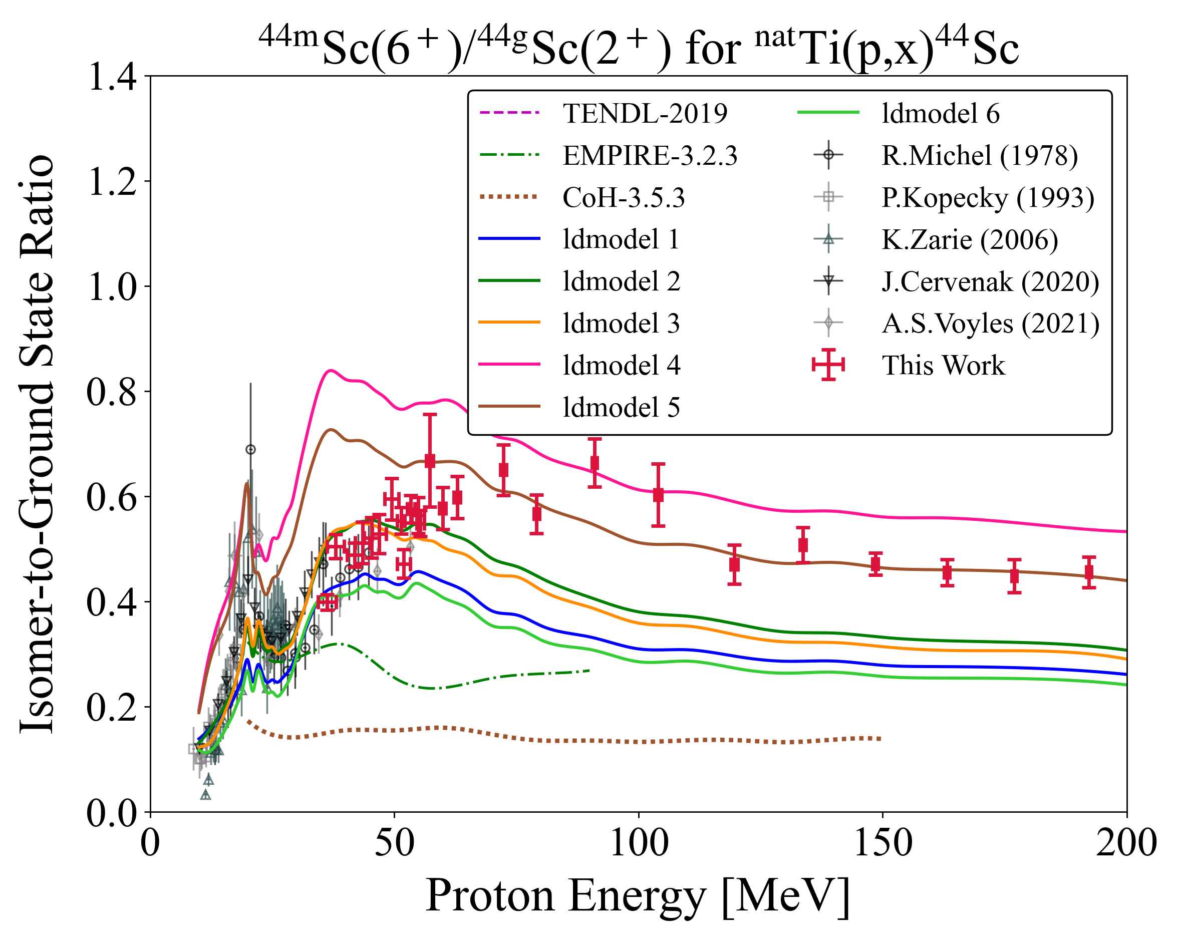
Figure 9: Experimental and theoretical results for the isomer-to-ground state production ratio for ^natTi(p,x)^44m/gSc. The predictions from all 6 TALYS level density models are shown, where ldmodel 1 is equivalent to the TALYS default.

Multiple experiments have measured this ratio previously for less than 50 MeV and there is agreement between the high-energy end of those measurements and the lowest-energy results of this work [52, 49, 54, 53, 33]. This new data extension could be used by the reaction modeling community to gain insight into angular momentum deposition over a broad range of incident particle energies.

The EMPIRE, CoH, and TENDL predictions for the isomer-to-ground state ratio are also shown in Figure 9 for comparison. The EMPIRE and CoH predictions markedly underestimate the ratio, however this result is a function of varying errors. In EMPIRE’s case, the ratio is incorrect due to an overestimation of ^natTi(p,x)^44gSc production (see Figure 24 in Appendix C) while the CoH misprediction is instead a function of underestimation for ^natTi(p,x)^44mSc production (Figure 24 in Appendix C).

In the compound peak energy region of the ^44m/gSc excitation functions (25–45 MeV), competition with other exit residual product channels is minimized. Hence the optical model impact and transmission coefficient effects are minimized and the isomer-to-ground state data in Figure 9 is largely a function of the level density of ⁴⁴Sc. Consequently, comparing the isomer-to-ground state predictions from TALYS’s numerous nuclear level density models is a conventional brief investigation of this data. These TALYS predictions are the remaining comparisons shown in Figure 9.

The ldmodel 1 in TALYS is the default Gilbert-Cameron constant temperature and Fermi gas model, but ldmodel 2, the Back-shifted Fermi gas model, appears to perform best in Figure 9 over the largest energy range. Though, it is perhaps noteworthy that the high-energy portion of the data is best reproduced by two of TALYS’s microscopic level density models - ldmodel 4 and ldmodel 5. The exact nature of these microscopic models, and all six models in total, can be reviewed in the TALYS-1.95 manual [34].

A single iteration of the Fox et al. [21] fitting procedure was additionally applied for ^natTi(p,x) to try and glean more insight on the effect of level density choice for the relevant nuclei. It was found that an overall best fit to the multiple observed residual product channels (see Table 4 for product list) was still achieved using ldmodel 2 but that an energy-dependent increase in the spin cut-off parameter was also included among the model adjustments. The spin cut-off increase, set by the procedure to begin globally at $E_{p}=40$ MeV in this case, broadens the width of the angular momentum distribution of the level densities involved in the ^natTi(p,x) reaction [34]. This adjusted best fit can be seen versus the unadjusted ldmodel 2 case for the isomer-to-ground state ratio in Figure 10. The mispredictions of the adjusted fit beyond $\approx$60 MeV are not necessarily unexpected since these calculations are significantly complicated due to a polyisotopic target. However, since special attention was paid to adjusting this ^44m/gSc ratio, the lasting mispredictions are likely more attributable to fundamental issues in the base pre-equilibrium model rather than parameter tuning.

It is interesting to observe that beyond $\approx$125 MeV, the ratio remains relatively constant, thereby indicating a limit to the maximum amount of angular momentum that can be imparted to the system. This is a reflection of the mechanics of the pre-equilibrium process.

This is evidently only an elementary investigation of the angular momentum in ⁴⁴Sc and neighbouring nuclei, and a detailed investigation is outside the intent of this paper. Altogether, this discussion is still presented to inform the value and scarcity of these types of ratio datasets over wide energy regions, and to provide motivation for further analysis.

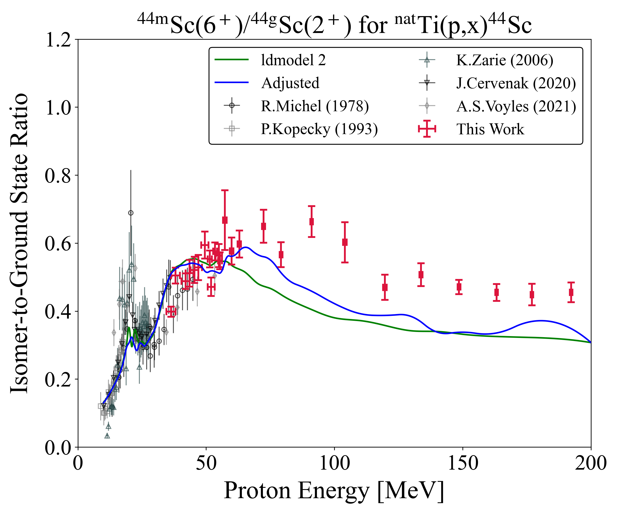
Figure 10: Comparison of the TALYS ldmodel 2 model prediction for the isomer-to-ground state production ratio for ^natTi(p,x)^44m/gSc with a TALYS fit using adjusted parameters, including a spin cut-off increase.

III.6 ^natCu(p,x) Cross Sections

The numerous ^natCu(p,x) cross sections measured here are in good agreement with the existing body of literature data and help to populate the more sparse regions of measurements between 100–200 MeV. Plots of these copper excitation functions are provided in Appendix C. Similar to the ⁷³Se results (Figure 7), the ^natCu(p,x) comparisons with existing data lend credence to our analysis methodology as well as our extensions to energy regions with no prior cross section measurements.

III.7 Predicted Physical Thick Target Yields

Instantaneous thick target yields for ⁷⁵As(p,x)⁷²Se, ⁶⁸Ge were calculated from the measured cross section results and are plotted in Figure 11. A comparison to the yields from earlier discussed established production routes for these generator nuclei in Section I are also included.

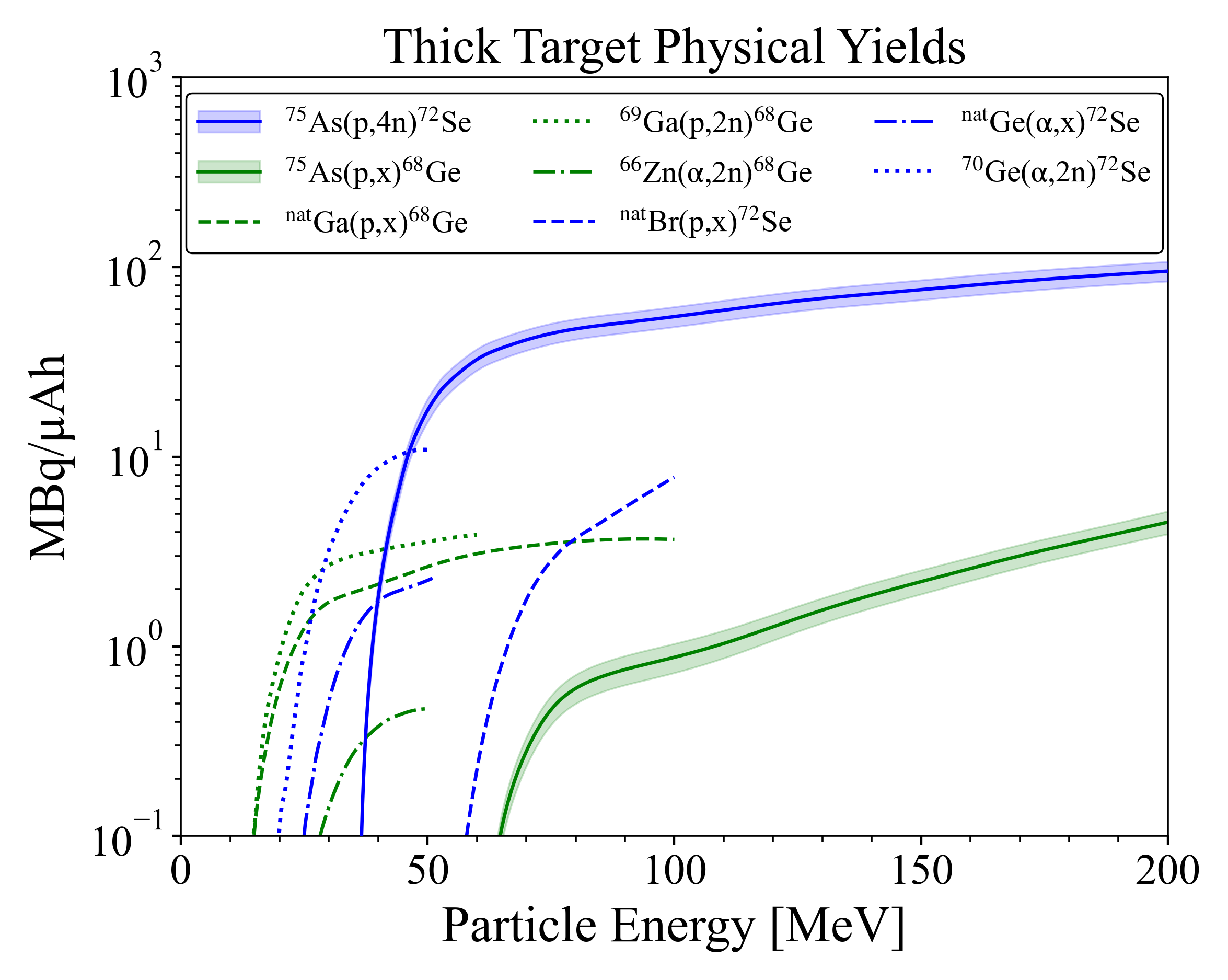
Figure 11: Yields for the PET generator radionuclides ⁷²Se and ⁶⁸Ge according to established production routes and the new arsenic-based routes measured in this work [42, 86, 87, 88, 89, 13, 90, 91, 92, 14, 93].

The data from TREND suggests that across all relevant incident particle energies beyond reaction threshold, the ⁷⁵As(p,4n)⁷²Se is the optimal production pathway to the ⁷²Se/⁷²As generator system. The arsenic target route offers an increase in yield of greater than an order of magnitude versus the current methods, while still affording radioisotopically pure production as best as possible. Specifically, no charged-particle production route to the ⁷²Se/⁷²As generator system is uncontaminated from ^75-73Se co-production. However, it is expected that ⁷²As will be efficiently separated from the parent ⁷²Se when needed, and that the co-produced ^75-73Se will also follow the chemical separation [9, 11]. Of course, any ⁷³Se contaminant is much shorter lived than ⁷²Se and can be decayed out to reach a more pure ⁷²Se starting condition regardless. Further, ⁷⁵Se production is energetically unfavorable in the p+⁷⁵As production conditions for ⁷²Se, meaning any in-grown ⁷⁵As prior to separation will be both minimal and stable. The ⁷⁵As(p,4n) pathway also avoids any potential long-lived ^74,73,71As contamination present from Ge target routes. In total, arsenic-based production of ⁷²Se gives the best chance to produce and collect a radiochemically-pure ⁷²As daughter.

It is seen that at incident proton energies nearing 200 MeV, the yield from ⁷⁵As(p,x)⁶⁸Ge can rival and exceed the production route based on already employed natural gallium targets. Specifically, Figure 11 predicts an $\approx$18% increase for the arsenic-based yield at 200 MeV (${4.5>3.8}$ MBq/$\mathrm{\SIUnitSymbolMicro}$Ah). Nevertheless, a p+⁷⁵As approach is expected to co-produce more stable germanium and ⁷¹Ge$\rightarrow^{71}$Ga contamination versus the p+${}^{\textnormal{nat}}$Ga route, leading to reduced ⁶⁸Ge specific activity. Arsenic targets would also introduce a need for additional, potential lossy, separation chemistries due to long-lived selenium and arsenic products not present from p+${}^{\textnormal{nat}}$Ga. Therefore, uprooting the successful established gallium route for arsenic is unwarranted. Still, this ⁷⁵As(p,x)⁶⁸Ge study gives valuable information in the context of total arsenic reactions, contributes to the knowledge base of the essential ⁶⁸Ge/⁶⁸Ga system, and demonstrates the importance of measuring these high-energy reactions, which can very easily produce large yields due to the long range of high-energy protons.

IV Charged-Particle Reaction Modeling

The effort to explore and improve the current nuclear reaction models for charged-particles, and perhaps more specifically charged-particles at high incident energies, is continued in this work. Explicitly, the TALYS residual product based fitting procedure presented by Fox et al. [21] is applied to ⁷⁵As(p,x) given the unique, large body of proton-induced data measured here.

The nine reaction channels ⁷⁵As(p,x)^75,73,72Se, ^74,73,71As, ⁶⁹Ge, ^68,67Ga were simultaneously used for the parameter adjustment investigation. ⁷³Se, ⁷³As, ⁶⁹Ge, and ⁶⁸Ga were considered as the most important fitting cases due to a combination of factors such as cross section magnitude, diversification of particle emission types, and impact on production competition with neighbouring nuclei.

IV.1 Deformation Effect of ⁷⁵As

While the cases of ⁹³Nb(p,x) in Fox et al. [21] and of ⁷⁵As(p,x) here have similar attributes - both utilize data from the same experiments, which cover the same energy range of interest, and both are monoisotopic targets in nearby mass ranges - the documented deformation of ⁷⁵As is a notable change from the spherical ⁹³Nb [94, 95, 96, 97]. This potentially introduces a complication to the direct application of the fitting procedure from Fox et al. [21]. Specifically, it would be necessary to address coupled-channels (CC) calculations or other angular momentum modifications to the typical spherically symmetric Hauser-Feshbach formalism prior to any further parameter changes [98].

The RIPL-3 imported TALYS value for the ⁷⁵As quadrupole deformation parameter is -0.25, which suggests a strongly oblate deformation [34, 99]. In fact, RIPL-3 lists strong oblate deformation for the arsenic isotopes $A=68-76$. While some experimental evidence supports these values for the neutron deficient cases and transitions around $N=Z$, it is quite rare that the neutron rich isotopes would demonstrate oblate rather than prolate deformation [100, 101]. An investigation using a Nilsson diagram gives further support that ⁷⁵As is actually prolate in nature. Finally, ENSDF and the original datasets incorporated into the structure evaluation provide experimental evidence of the prolate condition for ⁷⁵As and actually list a quadrupole deformation parameter of +0.314 (6) [94]. This prolate value appears to be both physically and historically more correct than the RIPL-3 $\beta_{2}=-0.25$ and is therefore taken as the ⁷⁵As deformation in the analysis that follows.

TALYS, however, does not include any deformation coupling schemes for arsenic isotopes and as a result, a spherical OMP basis is used in the predictive calculations, thereby potentially neglecting a significant physics aspect of the problem. It was therefore necessary to manually create a coupling scheme to see whether this has an effect on final results. Yet, the level scheme of ⁷⁵As does not present any ideal vibrational or rotational bands for coupling and its deformation is very likely either soft vibrational or soft rotational [102, 103].

On further examination, the $3/2^{-}$ ground state with the $5/2^{-}$ level at 279.543 keV and the $7/2^{-}$ level at 821.620 keV appear to form a rotational band. The $5/2^{-}$ level shows the expected strong $\gamma$-ray transition ($I_{\gamma}=100.0\ (5)\%$) of M1 character to the ground state, while the $7/2^{-}$ excited level shows both a strong E2 transition to the ground state ($I_{\gamma}=100.0\ (15)\%$) and weaker M1 transition to the $5/2^{-}$ level ($I_{\gamma}=9.6\ (11)\%$), generally in line with behaviour expected from a rotational band. Further, the $7/2^{-}$ E2 transition is 23.0 (24) Weisskopf units [104], providing evidence for its collective behaviour. This three-level rotational band coupling scheme was added to TALYS.

It was also noticed that the neighbouring nuclei ^76,74Se and ^76,74Ge demonstrate vibrational character [105, 106] and have vibrational coupling schemes implemented in TALYS for CC calculations (⁷⁶Ge has actually recently been shown as rigid triaxially deformed [107]). These neighbouring properties provide motivation to model the arsenic target as soft vibrational rather than rotational.

Unfortunately, TALYS’s implementation of the ECIS-06 code for optical model and CC calculations is unsuited for a pure vibrational coupling scheme for odd-Z nuclei, and the weak-coupling model has to be used in such cases. Moreover, the only odd-Z nucleus with any sort of vibrational deformation file in TALYS is ²⁴¹Am, where vibrational collectivity is built on top of rotational character. Therefore, taking the ²⁴¹Am deformation formatting as a guide, a weak vibrational band consisting of the ⁷⁵As $9/2^{+}$ (303.9243 keV), $5/2^{+}$ (400.6583 keV), and $1/2^{+}$ (860.0 keV) levels were added to a second created coupling scheme including the prior discussed rotational band. In this suggested vibrational band, the $1/2^{+}$ level is dominated by transition to $5/2^{+}$, which then has an E2 transition to the $9/2^{+}$ of 76.4 (25) Weisskopf units [104]. The $9/2^{+}$ de-excitation is dominated by E3 decay to the ground state. This mixed rotational+vibrational coupling scheme was also added to TALYS.

Elsewhere, this treatment for adjusting the global spherical optical model by a CC approach to implement a deformed optical model for ⁷⁵As calculations has been used in Shibata et al. [103] and Kawano [102]. The Shibata et al. [103] work is an evaluation of neutron nuclear data on ⁷⁵As up to 20 MeV for JENDL-4 and uses a similar rotational coupling scheme to the one presented here but substitutes the $5/2^{-}$ level at 279.543 keV with a $5/2^{-}$ level at 572.41 keV. Shibata et al. [103] uses the quadrupole deformation parameter $\beta_{2}=-0.19$ within a rigid-rotator model. In their evaluation, they found it necessary to additionally tune the matrix element parameter as well as the pickup and knockout contributions for their pre-equilibrium model relevant to the residual product cross sections of (n,$\gamma$), (n,p), (n,2n), and (n,$\alpha$). However, the JENDL-4 evaluation still found limited success in fitting the ⁷⁵As(n,p) channel after accounting for both deformation and pre-equilibrium changes. Shibata et al. [103] considered other solutions attempts that included level density and optical model parameter changes concerning both ⁷⁵As and ⁷⁵Ge but could not simultaneously improve the (n,p) channel while maintaining good global behaviour elsewhere.

Kawano [102] performed their CC calculations using the CoH reaction code and probed the collectivity effects in ⁷⁵As for incident neutrons. They explored the total and some close-to-target residual product cross sections up to 20 MeV, similar to Shibata et al. [103]. In comparison to ENDF/B-VII.0 results, the Kawano [102] calculations demonstrated improvement in reproducing the total cross section but did require model parameter adjustments for the individual reaction channels, not always yielding satisfactory results. Kawano [102] used the RIPL-3 suggested strong oblate deformation of arsenic.

In this p+⁷⁵As modeling work, the CC calculations in TALYS for arsenic, when invoking either the custom rotational+vibrational deformation or the custom pure rotational deformation scheme, together with the ENSDF-accepted prolate deformation parameter $\beta_{2}=+0.314$ (6), proved to have minimal impact on the predictions for residual product excitation functions. Any alterations that were present were not seen to be consistent improvements versus the default spherical optical model calculations. This is not an entirely unusual result given the higher energies under consideration and the overall expected lower level of collectivity for this target nucleus. It should be noted that this is not an exhaustive investigation of arsenic deformation, CC calculations, or collectivity models, and no structure or theory statements can be made. This result is only a statement of the sensitivity of the modeling under the conditions of this work.

Given the observed unremarkable changes, the inability to disentangle effects of CC calculations from more dominating level density, optical model, and pre-equilibrium parameter adjustments, and the imperfections of previously established deformed fitting approaches, the decision was made to treat ⁷⁵As spherically within TALYS and implement the fitting procedure from Fox et al. [21] identically.

IV.2 Fitting Procedure Applied to ⁷⁵As(p,x)

Firstly, the application of microscopic level density models proved beneficial as compared to the default phenomenological Gilbert-Cameron constant temperature model or the placement of compound peak centroids. However, it was seen that no one microscopic level density model best reproduced the excitation functions across all the observables. Instead, level density calculations from Goriely’s tables using the Skyrme effective interaction (ldmodel 4) [108] proved to be most accurate for the close-to-target residual products, and specifically for ^72-76Se and their competition with close-to-target arsenic products. Yet, applying ldmodel 4 to all nuclei involved in ⁷⁵As(p,x) created pre-equilibrium tails biased too high above the experimental data for Ga, Ge, and other $\alpha$-emission residual product excitation functions farther from the target. Conversely, it was observed that the temperature-dependent Hartree-Fock-Bogolyubov level density calculations using the Gogny force (ldmodel 6) [109] did not suffer from the magnitude bias problems in the far-from-target channels, but failed to model the close-to-target Se and their competing products unlike ldmodel 4. Therefore, two microscopic level density models were used, where ldmodel 4 was applied to the aforementioned grouping of selenium nuclei and ldmodel 6 was applied for all else. Further details of these level density considerations can be reviewed in Section IV.2.1.

The pre-equilibrium parameter adjustments in the next portion of the procedure were indeed found to follow the systematic trend described in Fox et al. [21], with M2constant=0.80, M2limit=3.9, and M2shift=0.55. Furthermore, the value for the constant of the proton and neutron single-particle level density parameter used for calculations of the exciton model particle-hole state densities was altered from its default Kph=15 to Kph=15.16. Other pre-equilibrium modeling changes were manipulations of the stripping and knockout reaction contributions for outgoing alpha, deuteron, triton, and ³He particles. These manipulations were performed using the TALYS Cstrip and Cknock keywords. The precise adjusted values can be viewed in Table 9 in Appendix D.

Subsequent iterative simultaneous tuning of optical model and individual level density parameters were needed to aid the compound reaction regime and to fix erroneous production competitions between clustered products.

The need for nuclide-specific level density changes arises from discrepancies between measured and modeled data where global changes to exciton or optical model parameters can not resolve the singular problems. These nuclide-specific adjustments were most evident for ⁷³As production, where both the adjusted fit to this point and the default calculation were nearly 200 mb smaller than the observed results. As in Fox et al. [21], these level density manipulations per nuclide could be performed with the TALYS ctable and ptable commands when microscopic level density models are implemented.

The effects of ctable and ptable to create an adjusted level density $\rho(E_{x},J,\pi)$ are explicitly given by,

$$\rho(E_{x},J,\pi)=\exp(c\sqrt{E_{x}-\delta})\rho_{mic}(E_{x}-\delta,J,\pi),$$ (2)

where ctable is the $c$ constant, ptable is the $\delta$ constant (denoted as the “pairing shift”), and $\rho_{mic}(E_{x}-\delta,J,\pi)$ are the tabulated microscopic level density calculations as a function of excitation energy $E_{x}$, angular momentum $J$, and parity $\pi$. The produced tables in TALYS have not been adjusted to experimental data and have $c=0$ and $\delta=0$ by default. The implementation of ctable and ptable under the definition of Equation (2) then provides necessary scaling flexibility at both low and high energies [34].

Since the production of ⁷³As is most heavily correlated with the neighbouring exit channels ^72,73Se and ⁷⁴As, the ctable and ptable effects on ⁷³As necessitated corresponding nuclide-specific level density changes in ^72,73Se and ⁷⁴As as well.

The most suitable optical model adjustments were found to be d1adjust n=1.75 and d1adjust p=1.55, which multiply the energy-dependent imaginary surface-central potential well depth for neutron and protons, respectively. These multiplicative changes lead to increased particle emission from the surface region of the nucleus, and thus to increased emission of high-energetic particles, particularly at lower incident proton energies. In turn, these alterations create a more pronounced pre-equilibrium spectrum that contributes additional production within the compound regions of residual product excitation functions and some additional production to their tails.

Although these are not unsubstantial multiplication factors from the default 1.0 values, the energy dependence of the surface potential means that the adjustment impact is large in the vicinity of low threshold channels for lower incident proton energies but becomes only a minor change above $\approx$50 MeV. This is mirrored by the volume potentials that increase and dominate absorption/emission as energies reach $\approx$50 MeV and beyond. For example, at $E_{p}=20$ MeV, the default imaginary surface-central potential well depth for protons on ⁷⁵As is 8.4 MeV while the adjusted well depth is 1.55$\times$ larger at 13.0 MeV. This 4.6 MeV difference is a relevant change around low residual product threshold energies but by $E_{p}=75$ MeV, this default versus adjusted well depth difference is reduced to just 1.5 MeV. The difference then falls below 1 MeV at $E_{p}=90$ MeV, and is reduced down to 0.1 MeV at $E_{p}=200$ MeV. Similar behaviour is true for the change to the imaginary surface-central potential well depth for neutrons. Furthermore, at $E_{p}=20$ MeV, the imaginary volume potential is $5-7\times$ smaller than the imaginary surface potential for both neutrons and protons in the adjusted case, but by $E_{p}=75$ MeV, the imaginary volume potential has grown to be $2-3\times$ larger. The imaginary volume potential becomes increasingly more dominant, growing to be $50-70\times$ larger by $E_{p}=200$ MeV.

It is possible that portions of the d1adjust changes should actually be substituted with changes to the imaginary surface diffusivity parameter, but this cannot be unambiguously determined using only residual product cross section data and instead requires angle-differential cross section information [110]. This limited diversity of high-$E_{p}$ fit data is a common theme that permeates the limitations of this approach to parameter adjustments as well as prevents much physical meaning to be gleaned from the modeling. These limitations are further explored in Section IV.4.

An additional increase to proton absorptivity and emissivity across a wider range of energies, to increase peaks and tails for numerous channels consistently, was still warranted by the experimental data. This was implemented with an increase to the imaginary volume potential well depth for protons by w1adjust p=1.21.

The default TALYS alpha optical model of Avrigeanu et al. [111] was deliberately chosen as it performed best for the considered As and Ge channels. The deuteron optical model of Han et al. [112] was applied instead of the default model from standard Watanabe folding [113]. This deuteron adjustment is minor ($\leq 5$ mb) compared to the alpha model effect but does better match the experimental peak and tail behaviour in observed residual product channels for $A\leq 72$.

Lastly, an additional minor nuclide-specific case for level density adjustments that became relevant as a result of iterating over the above parameter changes was ⁷¹As. This adjustment included corresponding small level density changes to ⁶⁸As, ⁶⁹Ge, and ⁶⁹Ga as a function of correlated production competition.

The lone prominent outstanding modeling discrepancy among the considered channels was an overprediction of ⁶⁷Ga production. It is likely that this difference represents a sensitivity limit for this fitting procedure through a manual approach. Moreover, given the massive parameter space for adjustments in TALYS, it is realistic that the fitting here ends in a local variance minimum, unable to perfectly match all prioritized ($\approx$15% of total cross section) and minor ($\leq 5$% of total cross section) residual products. We can correct for this ⁶⁷Ga error by reducing the nuclide-specific level density, but this change is likely a compensating correction in this context and does not contribute to any increase in predictive power.

All parameter changes creating this total adjusted fit are given in Table 9 in Appendix D. Figure 12 presents the adjusted fit compared to the default TALYS calculation for the nine considered reaction channels up to an incident proton energy of 200 MeV.

Overall, we put forth a large number of level density scalings, either directly or as a correlation consequence, and though this is not unexpected given the prior lack of data and ambiguity for the reactions and energies of interest [109, 114], it is important to reflect on the intricacies of performing such a number of scalings. This discussion is presented in Section IV.2.1.

Additionally, context for our suggested parameter adjustments can be gleaned from the “best” parameters file for n+⁷⁵As included with TALYS-1.95 [34]. This “best” parameterization contains multiple level density scalings (with the back-shifted Fermi gas model as a base) in addition to multiple optical model real potential radii and diffusivity adjustments, some of which reach upwards of 11% changed from default and are made energy-dependent. Similar stripping and knock-out contributions to our suggested adjustments in this work exist as well in the “best” file. Overall, our adjustments generally work to avoid potential unphysical changes to geometry parameters and the real potential instead to focus on the imaginary potential. This focus is likely more appropriate for high-energy residual product cross section datasets versus the lower-energy scattering and resonance data important to the development of the “best” n+⁷⁵As parameters.

(a)

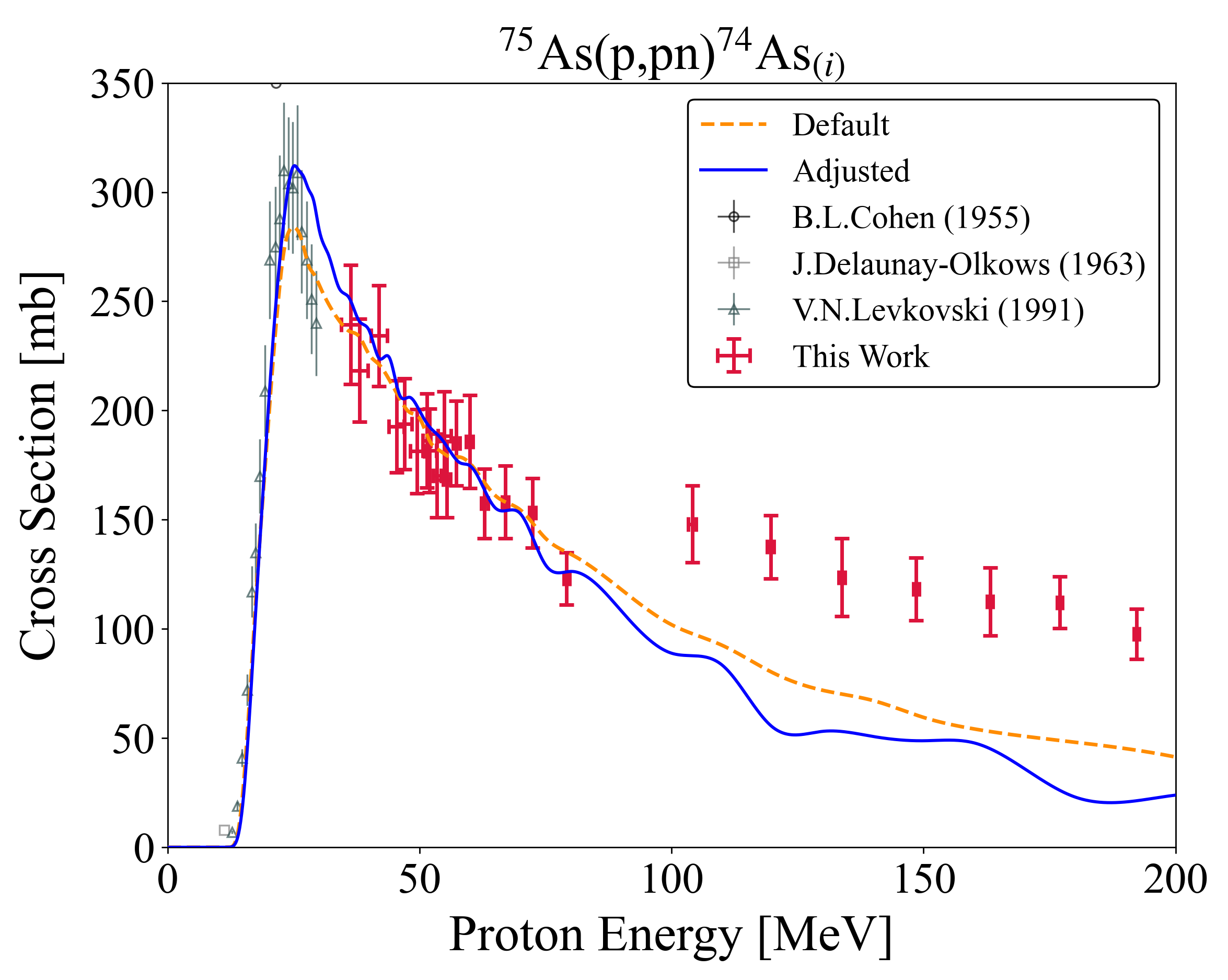
(b)

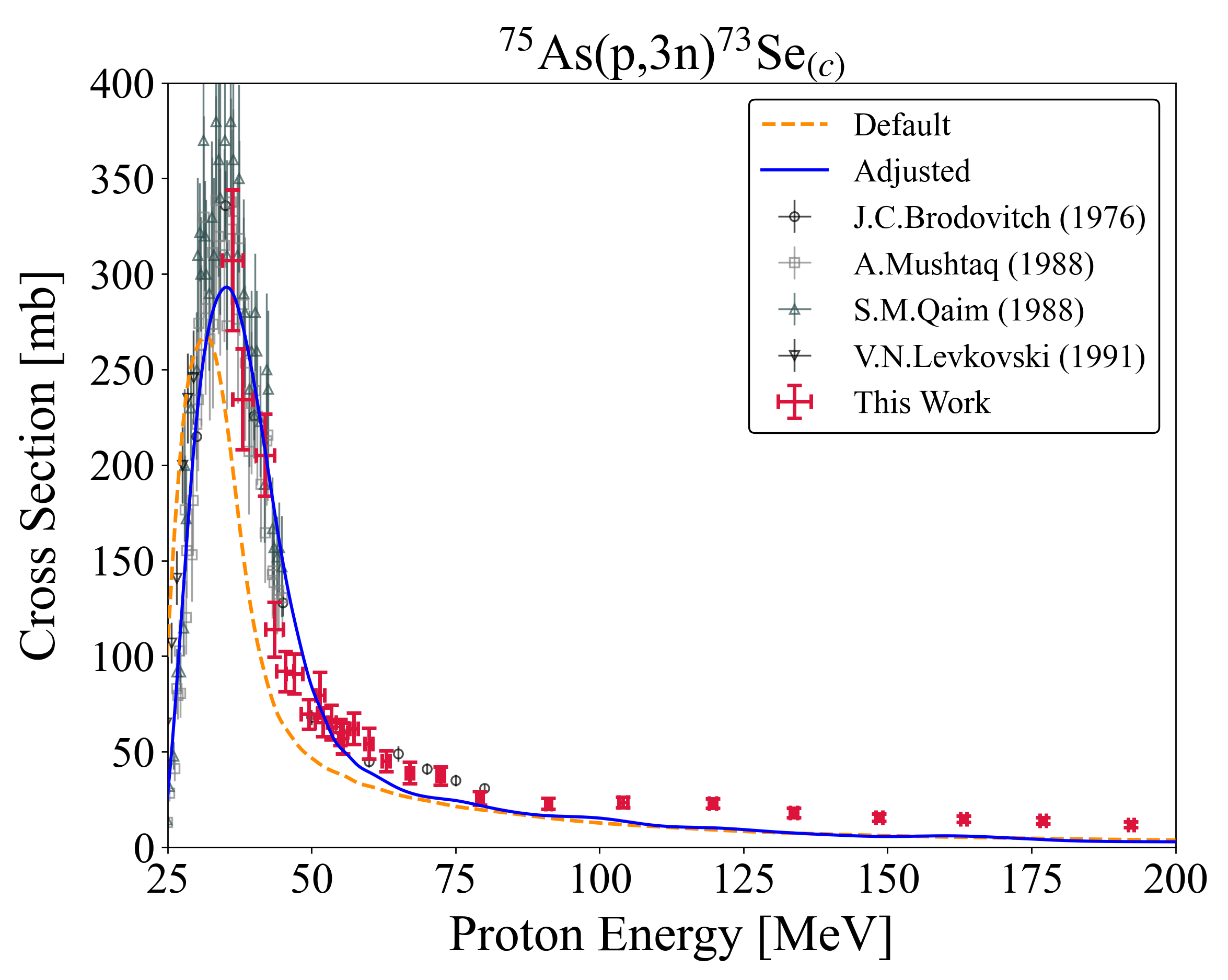
(c)

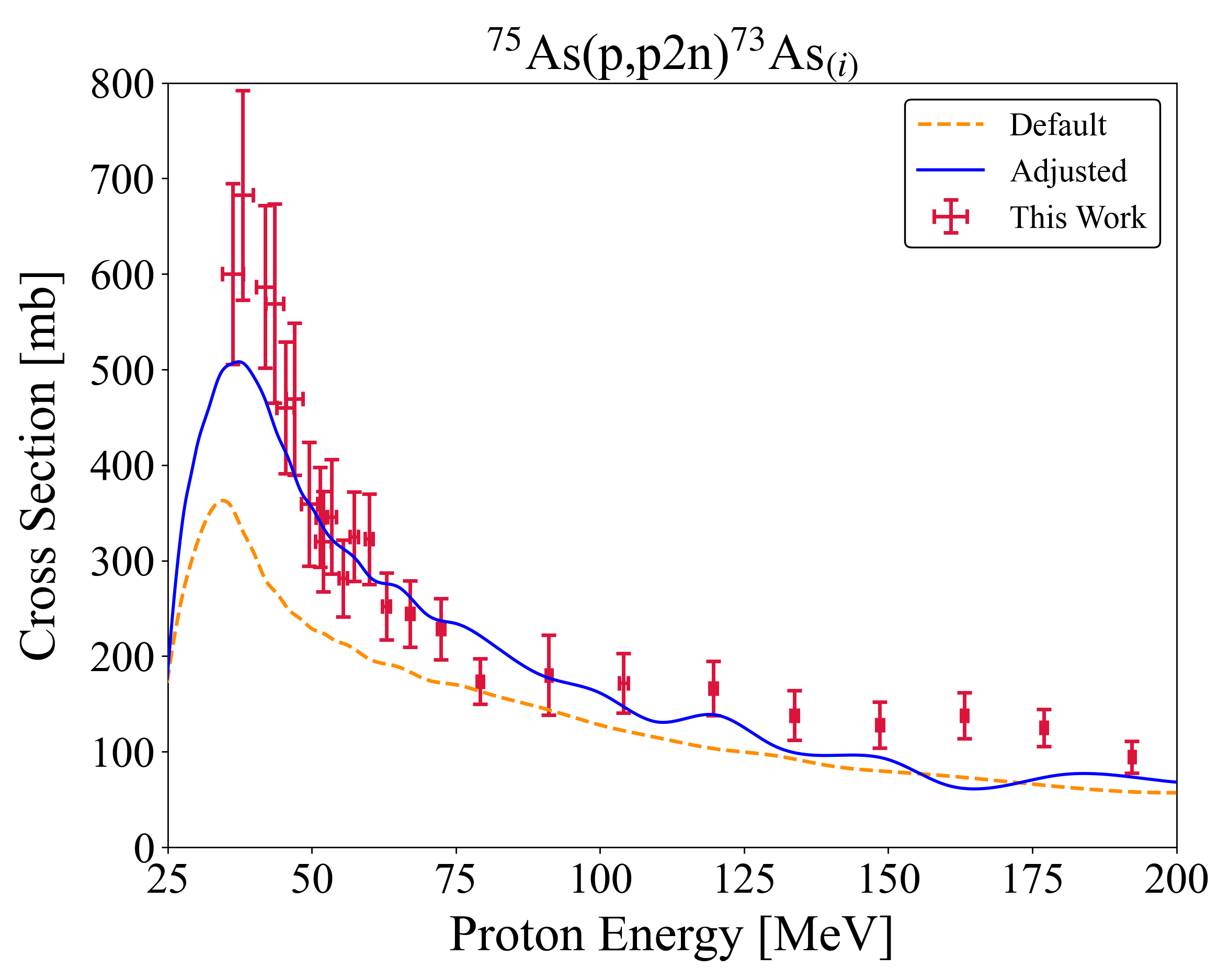
(d)

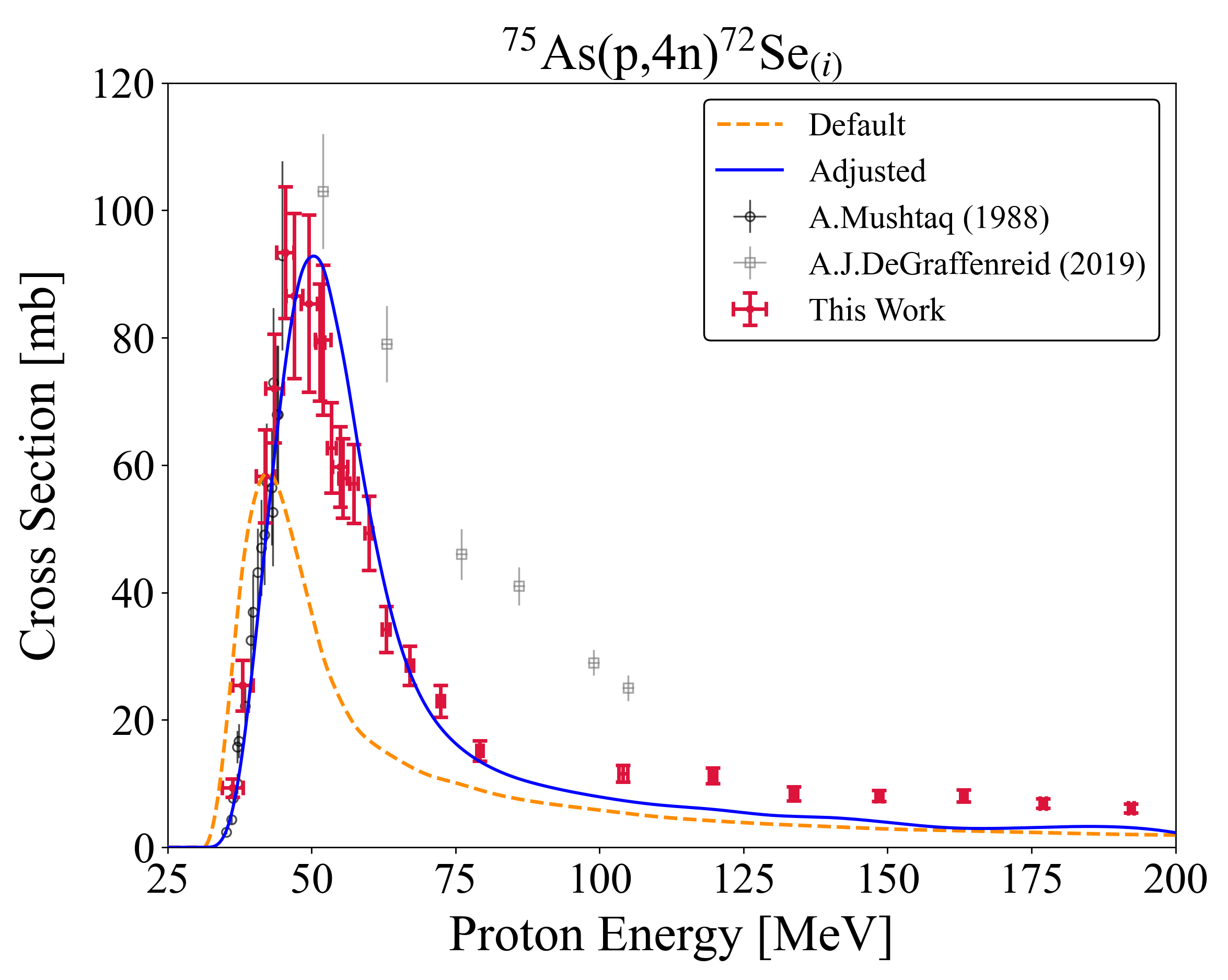
(e)

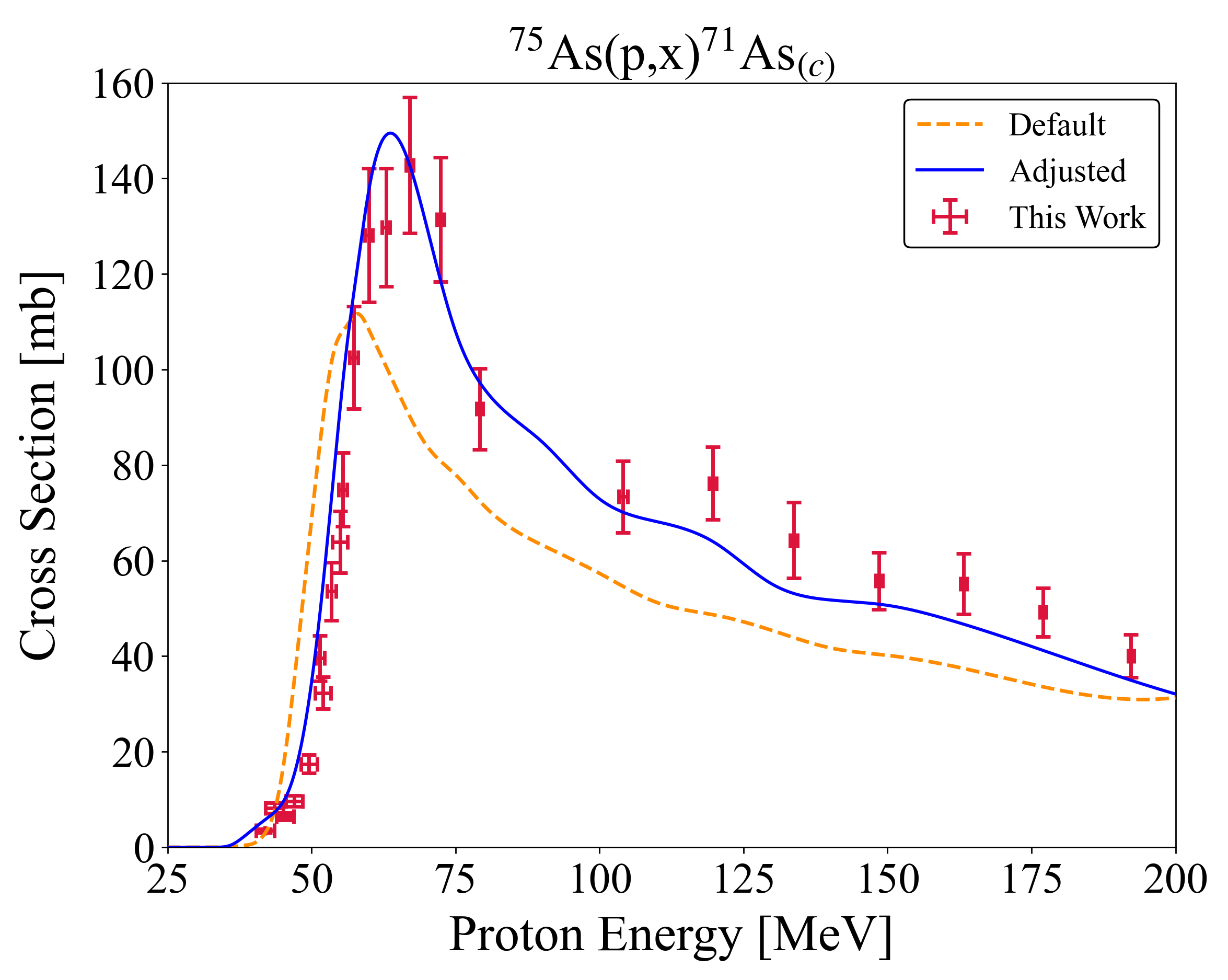
(f)

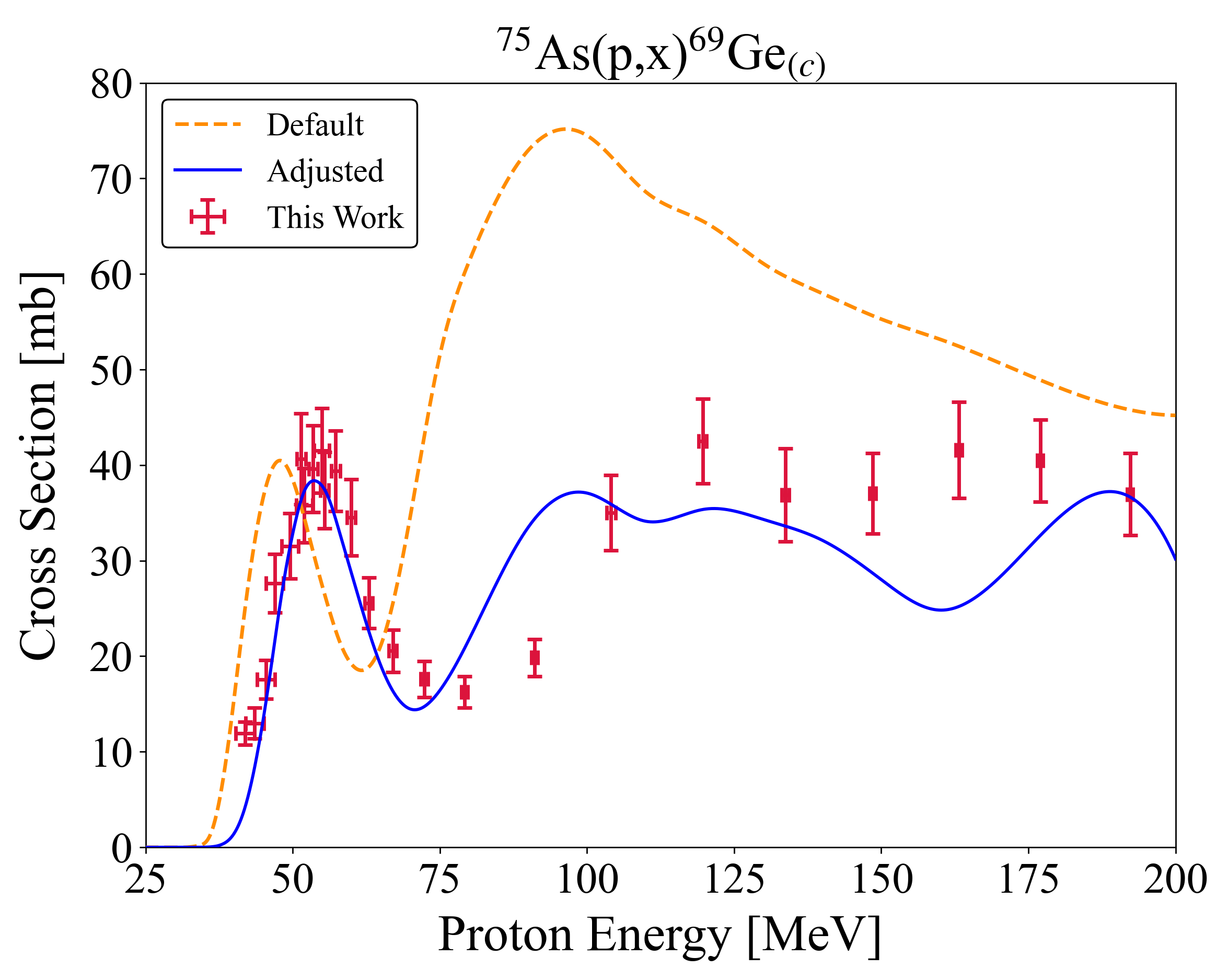
(g)

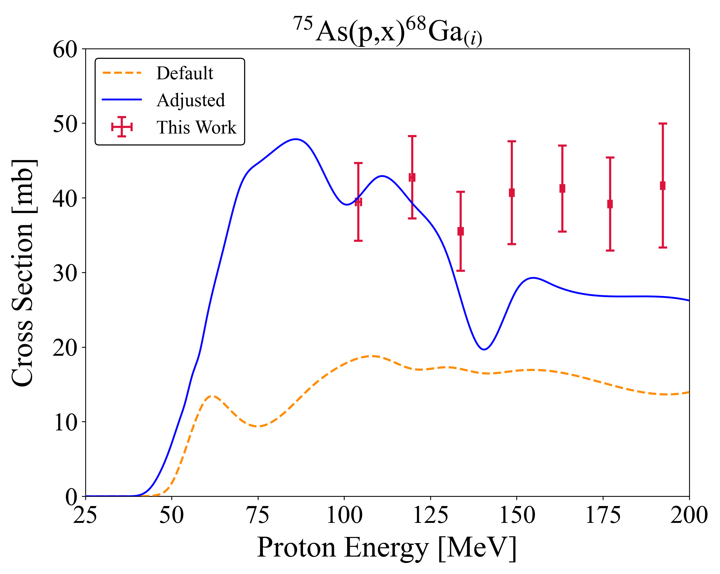
(h)

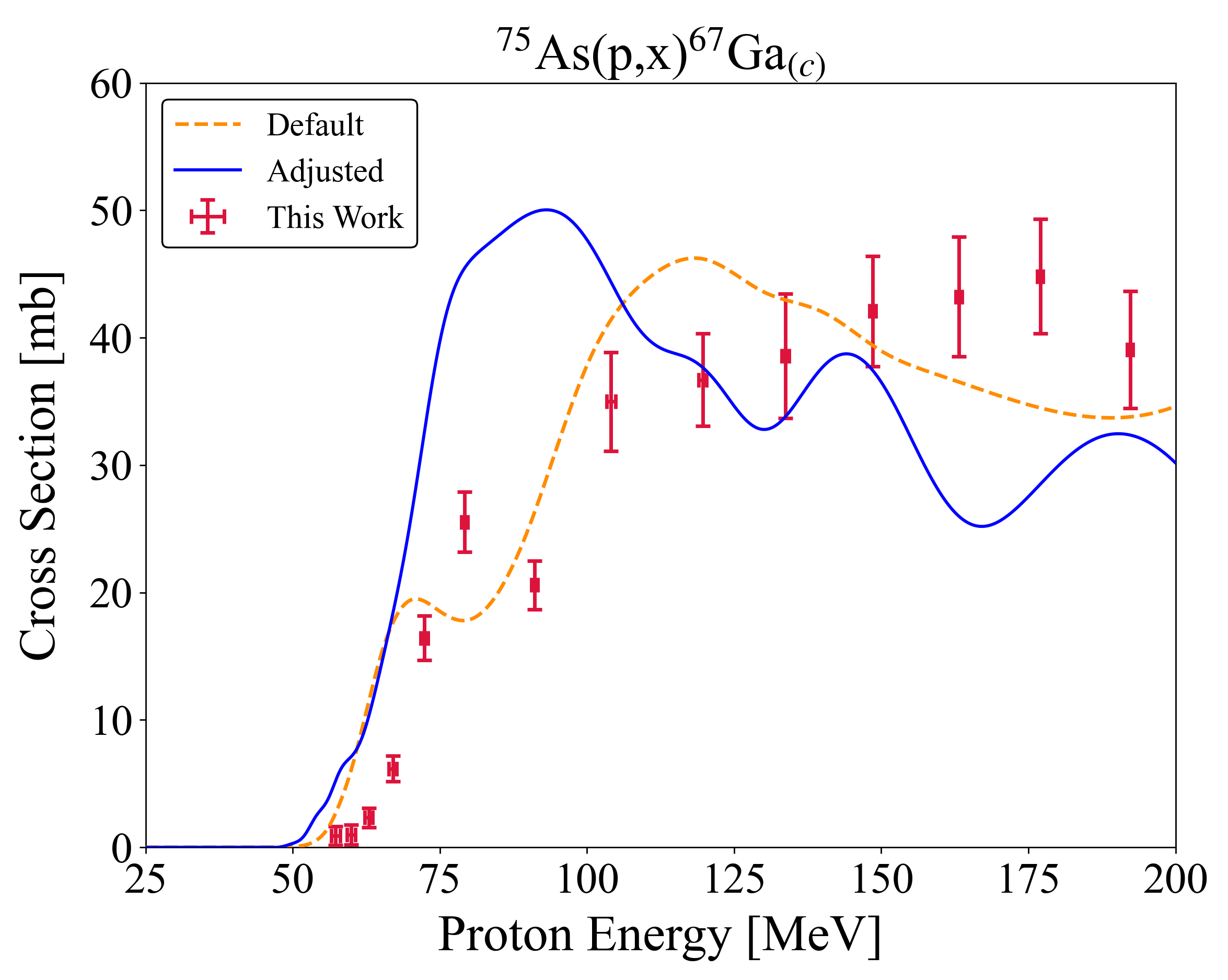
(i)

Figure 12: TALYS default and adjusted calculations for residual products of proton-induced reactions on arsenic up to 200 MeV.

IV.2.1 Level Density Adjustments

Figure 13 directly shows the magnitude of all manually adjusted level density cases with reference to the base ldmodel choice. The total level density of ⁷³As has been significantly increased (Figure 13c), as warranted by the experimental data, while a significant decrease is seen in ⁶⁷Ga although for less direct reasons (Figure 13i).

The recommendation of these many level density changes is substantiated by the global fit success seen in Figure 12 and described in Section IV.3 but still requires more scrutiny. Furthermore, it is necessary to, at minimum, consider the impact of these level density changes on the residual product channels for which there were no experimental data and were unaccounted for either independently or cumulatively throughout the fitting procedure. Specifically, due to limitations of the activation technique to measure stable or some very-short lived nuclei production, the ⁷⁵As(p,x)⁷⁴Se, ^74-70Ge, and ^73,71-69Ga channels, for $A>65$ and $Z>30$, were hidden from the fitting observations. Accordingly, it is essential to have a “performance check” for these hidden channels, where the TALYS default and adjusted fits can be compared to monitor for any egregious shape or magnitude changes brought on by the level density adjustments.

The fit performance for stable ⁷⁴Se is of particular interest since had there been experimental data, the channel would have been one of the prominent excitation functions for the fitting procedure. This ⁷⁴Se performance check is given in Figure 14 and the difference between the default and adjusted is certainly acceptable.

In the unobserved Ge and Ga channels, there continues to be no obviously incorrect changes from the default to adjusted cases. Magnitude differences for most of these products reach $\approx$5-7 mb and excitation function shape continuity is maintained within expectations. The adjusted ⁷⁰Ge production is the most significantly changed hidden channel from default, with a maximum difference of $\approx$40 mb in the compound peak region. Therefore, when confined to residual product datasets, there are no obvious indications that the bulk of the level density adjustments made here are not viable. Even if new experimental data were to be collected for these “hidden” channels, which disagreed with the adjusted fit, it is likely that since no drastic changes have been made, the parameters can be properly updated to include the new information.

It is also worth remarking that using multiple level density models in this work is not a qualification or statement that one model more accurately reflects physical behaviour. Instead, we can only conclude that multiple level density models, and nuclide-specific changes, were simply scalings needed to best match the available experimental data, which has been seen in other work as well [114, 115]. There is likely no clear physical insight about the models that can be taken from these fits alone.

Perhaps some of the need for scaling is due to inconsistent or lacking discrete level data that feeds into the level density models. The residual products of interest generally exist off the line of stability and resonance parameters are unknown [115, 116, 117]. In ⁷⁰As and ⁷²As, only 68 and 65 experimental discrete levels, respectively, as stored in the RIPL-3 database, inform the level density calculations [34]. This is compared to isotopes such as ^71,73,75As where over 120 experimental levels each are used.

A similar pattern exists for ⁷²Se where only 52 experimental discrete levels inform calculations, as compared to much more well-characterized ^73-76Se isotopes. If there are missing levels relatively low in the level scheme, then the level density model may be adjusted to the wrong number of assumed complete levels. This lack of structure data exists for ^66,67Ge and ^66,68Ga within their respective isotope chains as well. Ultimately, it is conceivable that incomplete structure data leads to numerous compensating level density effects in this mass region, which may themselves be a key contributor to the adjusted scalings as opposed to any inherent issues with the models [115, 116, 117].

It is also possible that a disregard of isospin effects in the current TALYS calculations, missing collective enhancement effects for nuclei far from stability, or deterioration of the microscopic level density models altogether at the high excitation energies relevant to this work, have prompted the need for the corrective scalings [117, 118]. A future experiment examining $\alpha$+⁷²Ge, which populates the same ⁷⁶Se compound system as p+⁷⁵As but with different isospin, could provide some additional information. Relevant future research may also include examinations of smooth transitions between different level density models as a function of mass difference from the target nucleus or separate structure-based level density model-mixing schemes. The implementation of different level density models in this manner merits specific interest because it has shown to be needed for p+⁷⁵As here and p+⁹³Nb in Fox et al. [21].

The overall viability of the level density adjustments in this modeling work in combination with the other modeling parameter changes are further justified in Section IV.3.

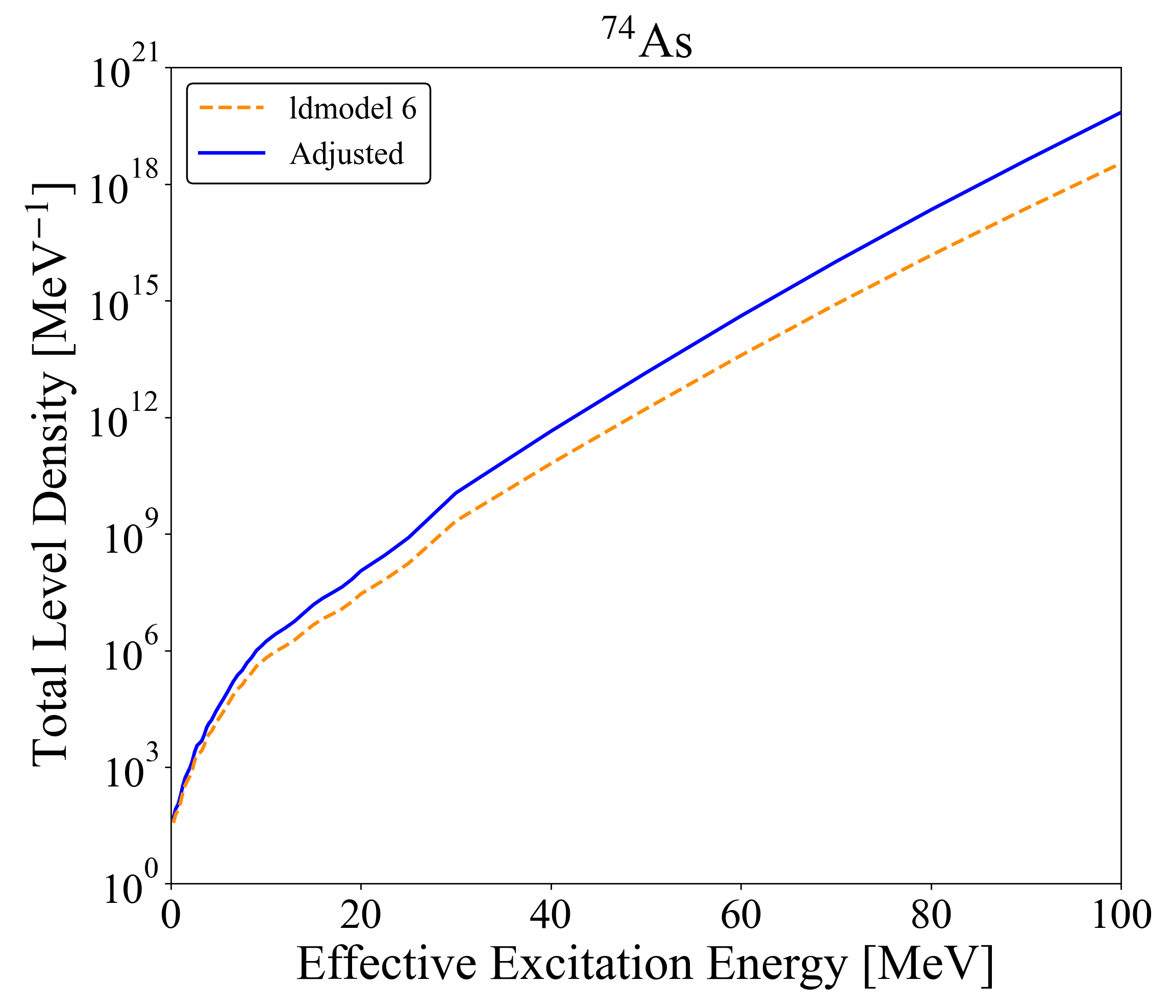
(a)

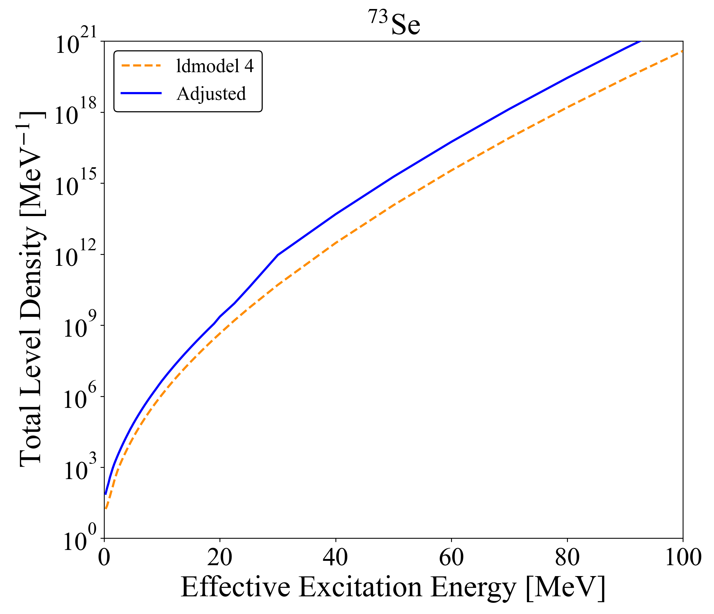
(b)

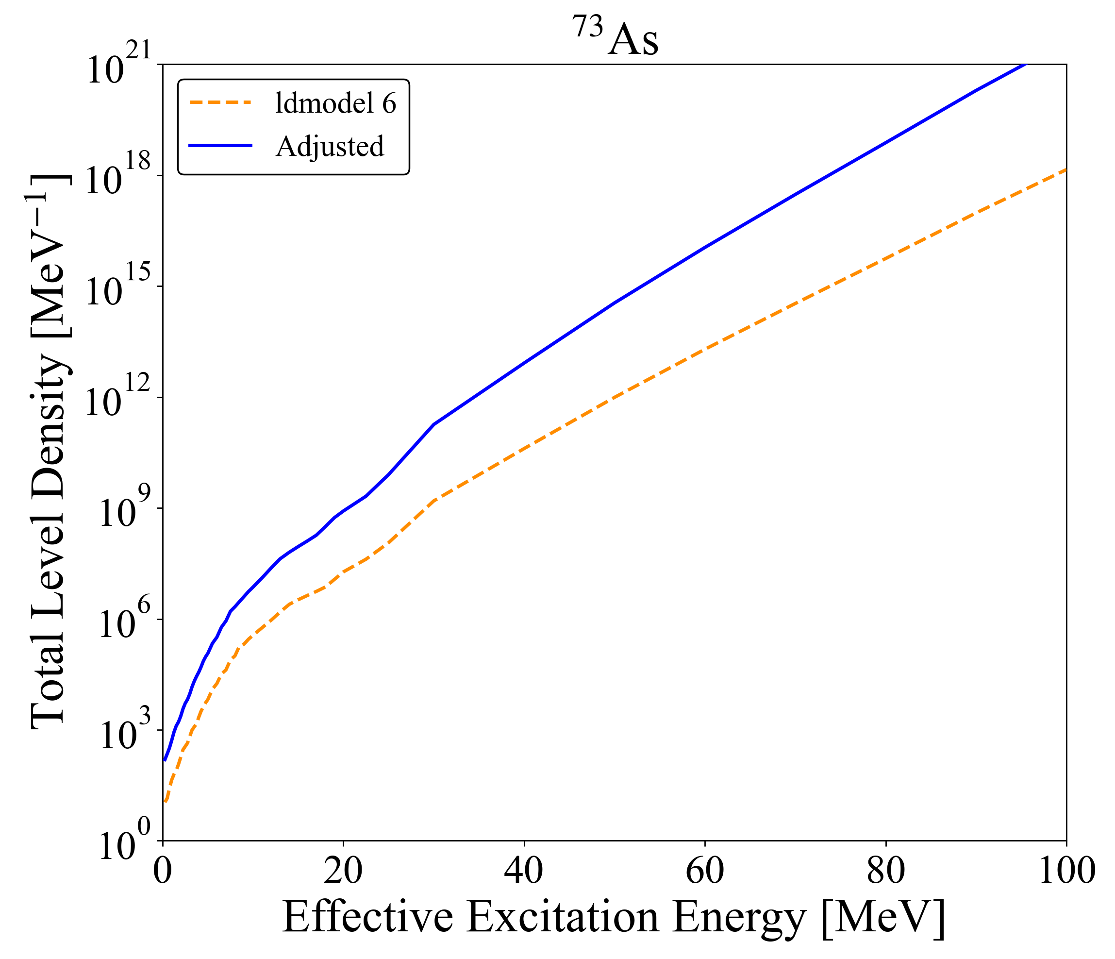
(c)

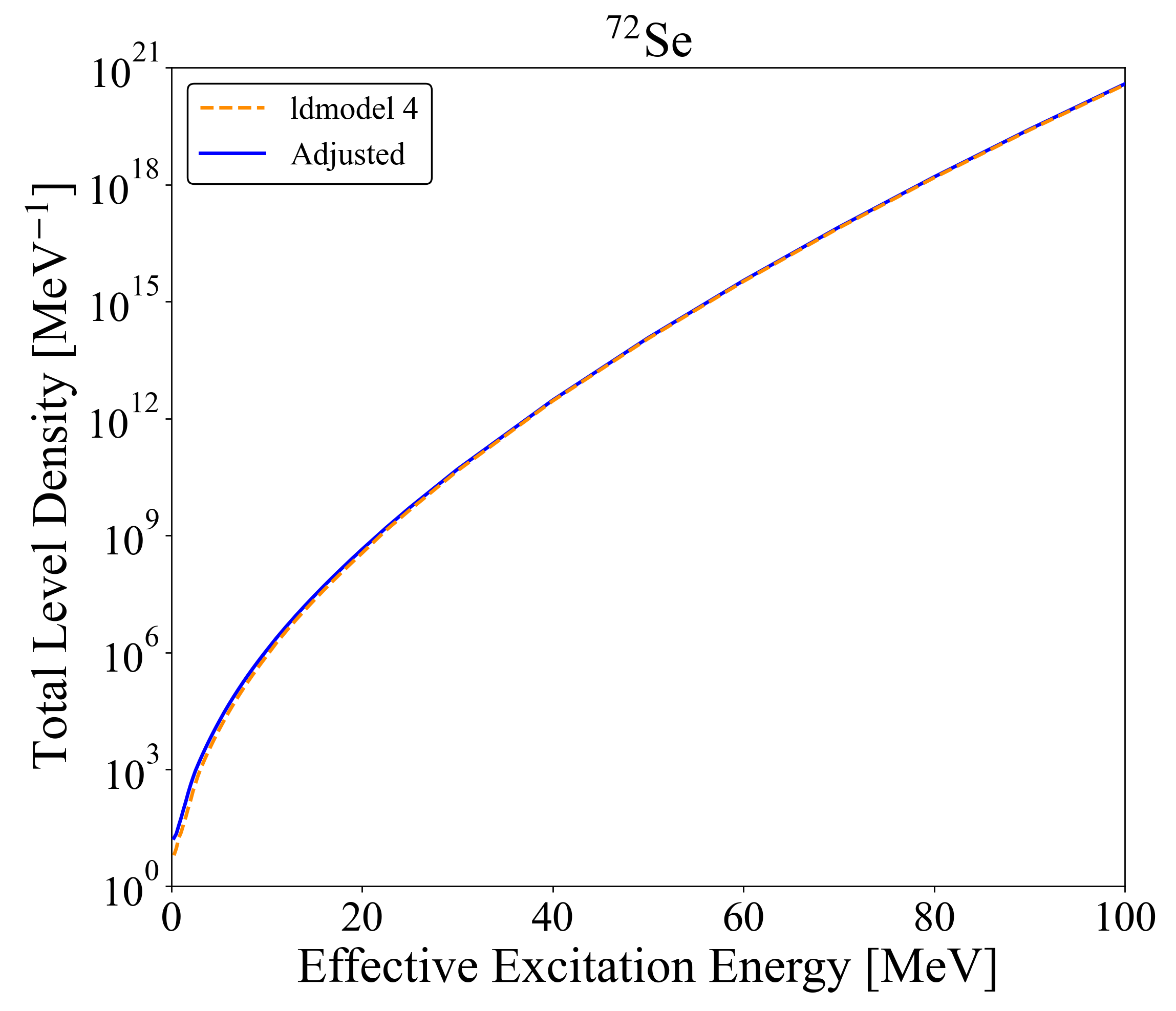
(d)

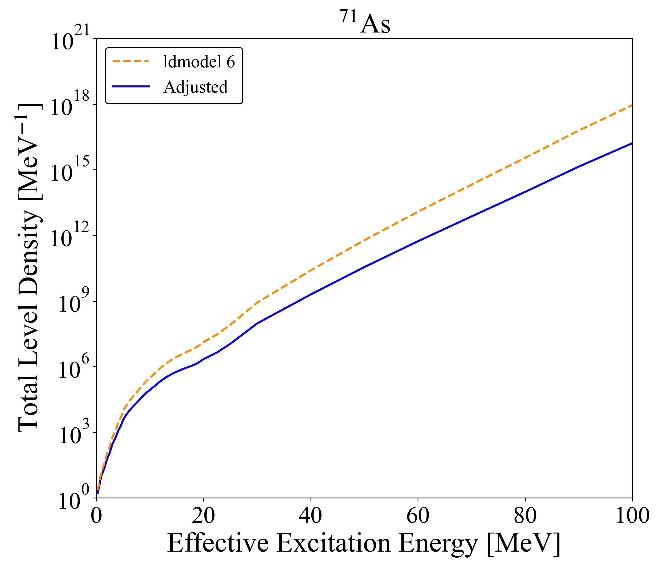
(e)

(f)

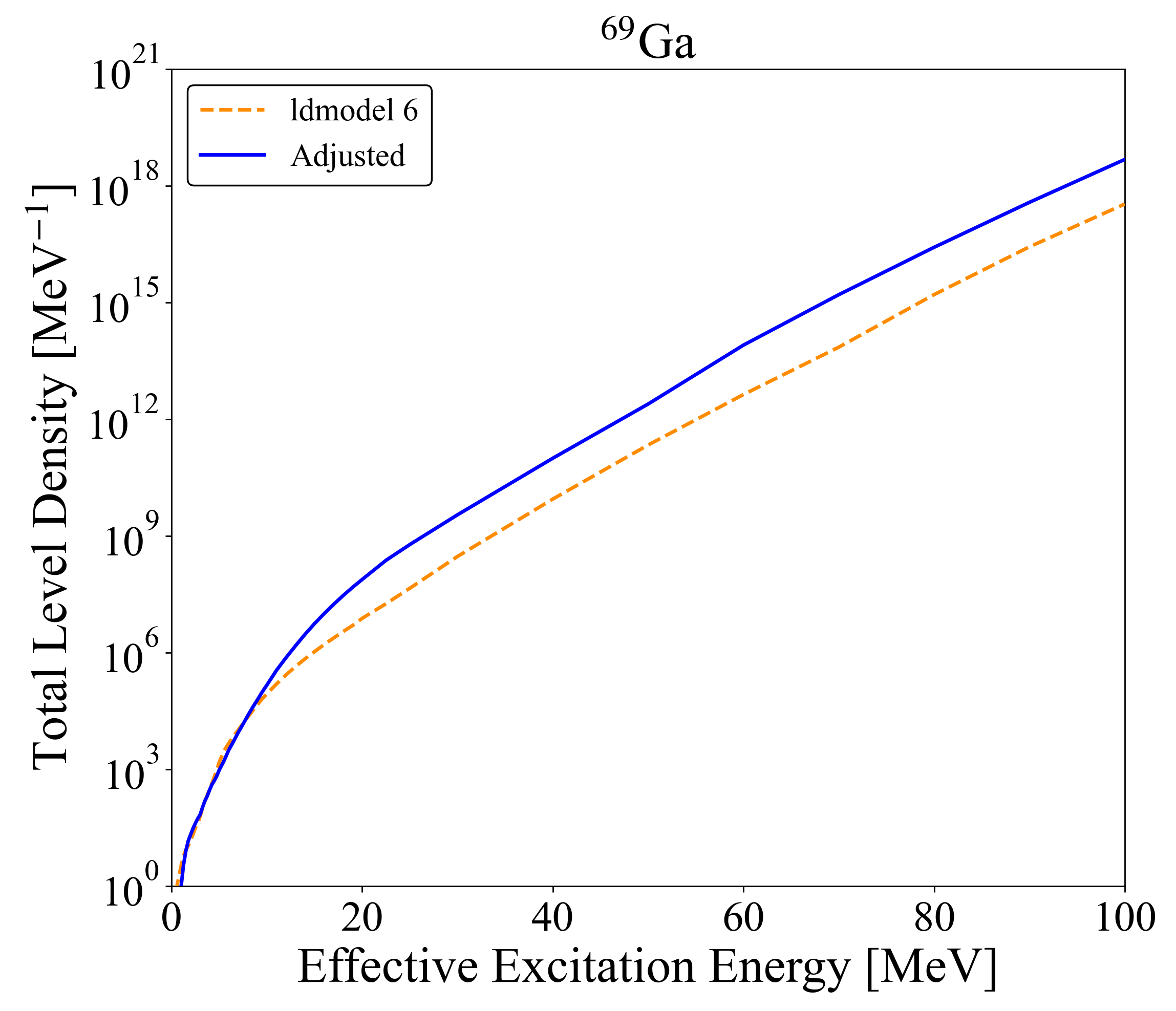
(g)

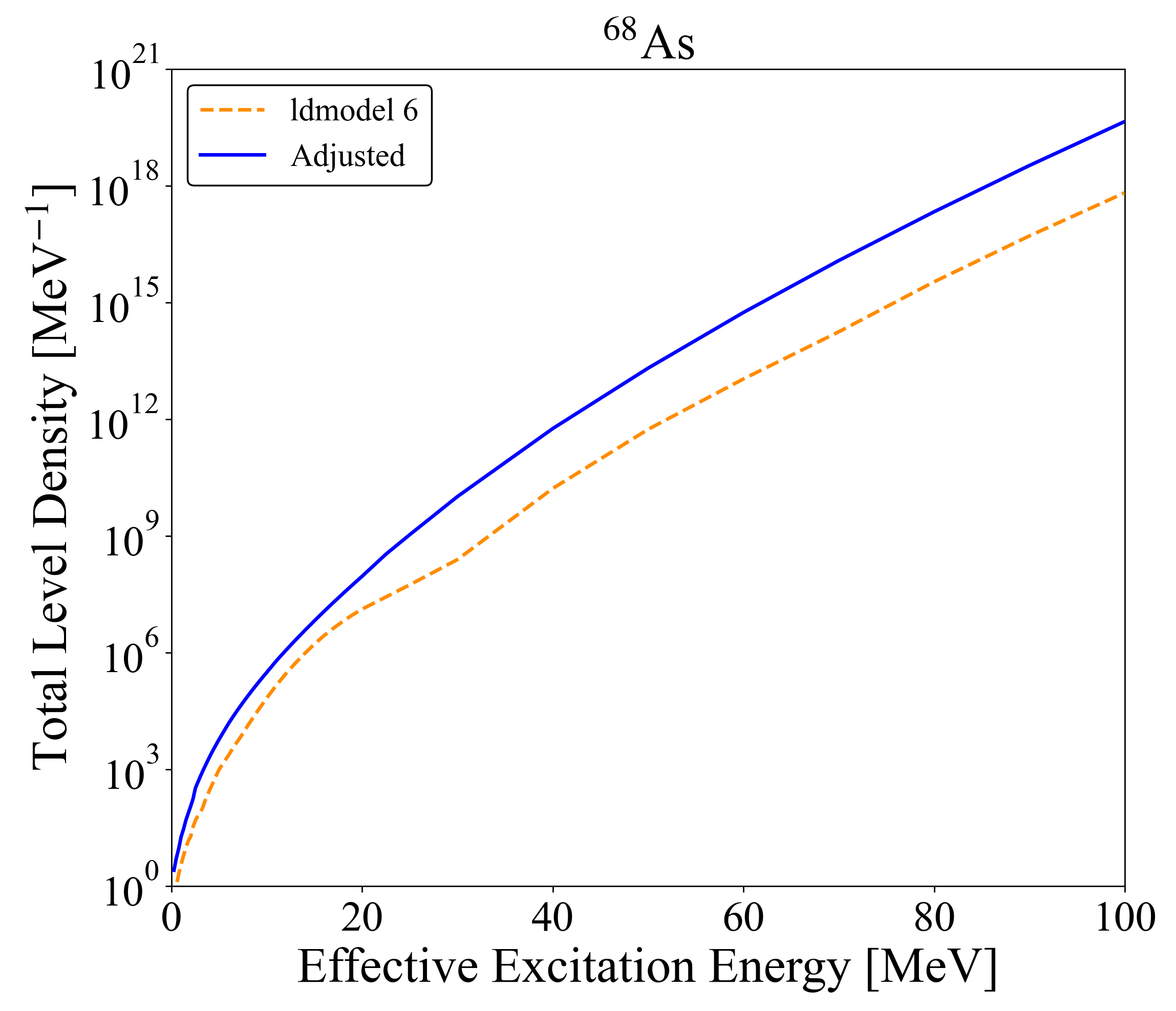
(h)

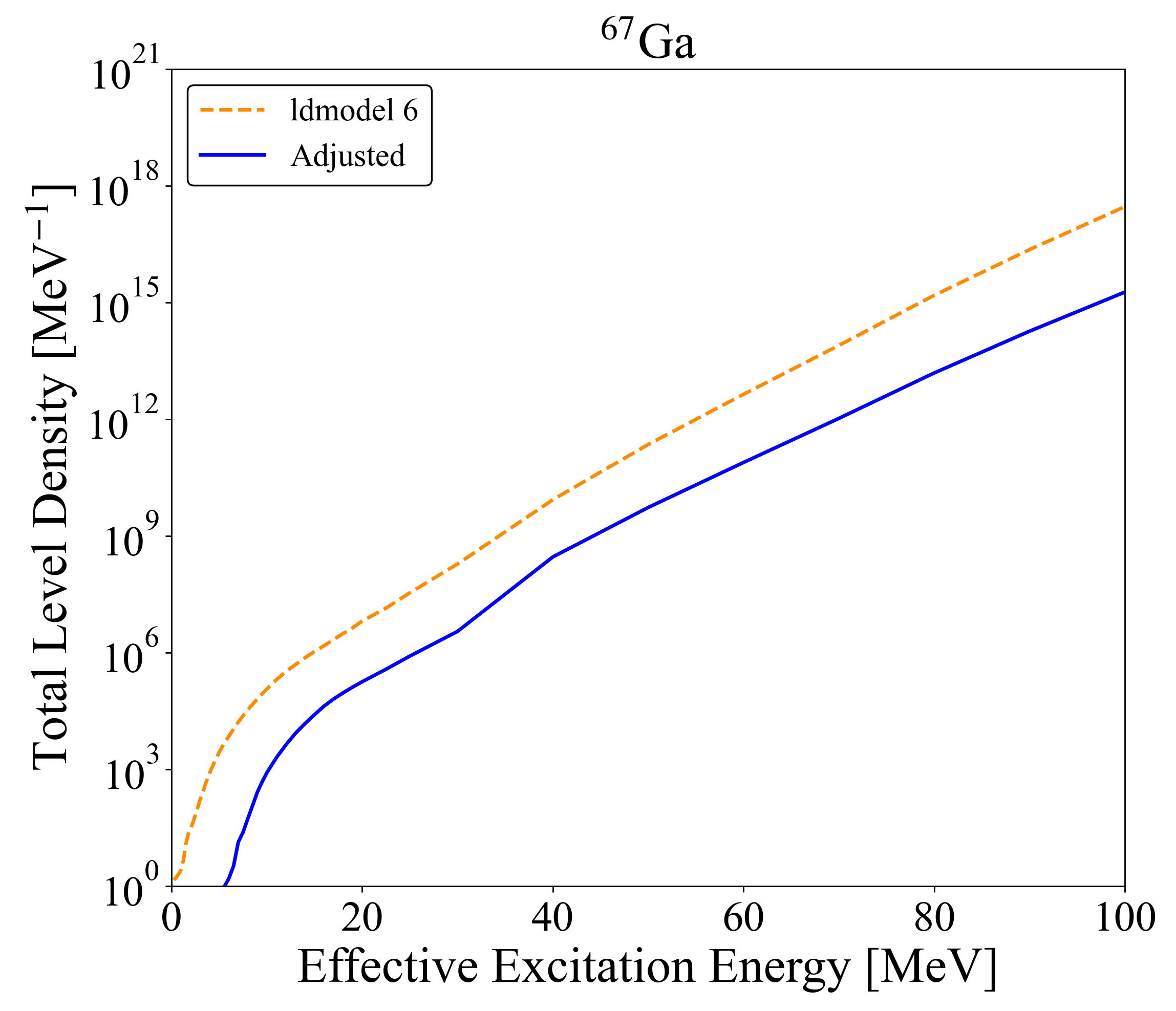
(i)

Figure 13: Magnitude of all level density scalings implemented as part of the global fitting procedure for residual products of proton-induced reactions on arsenic up to 200 MeV.

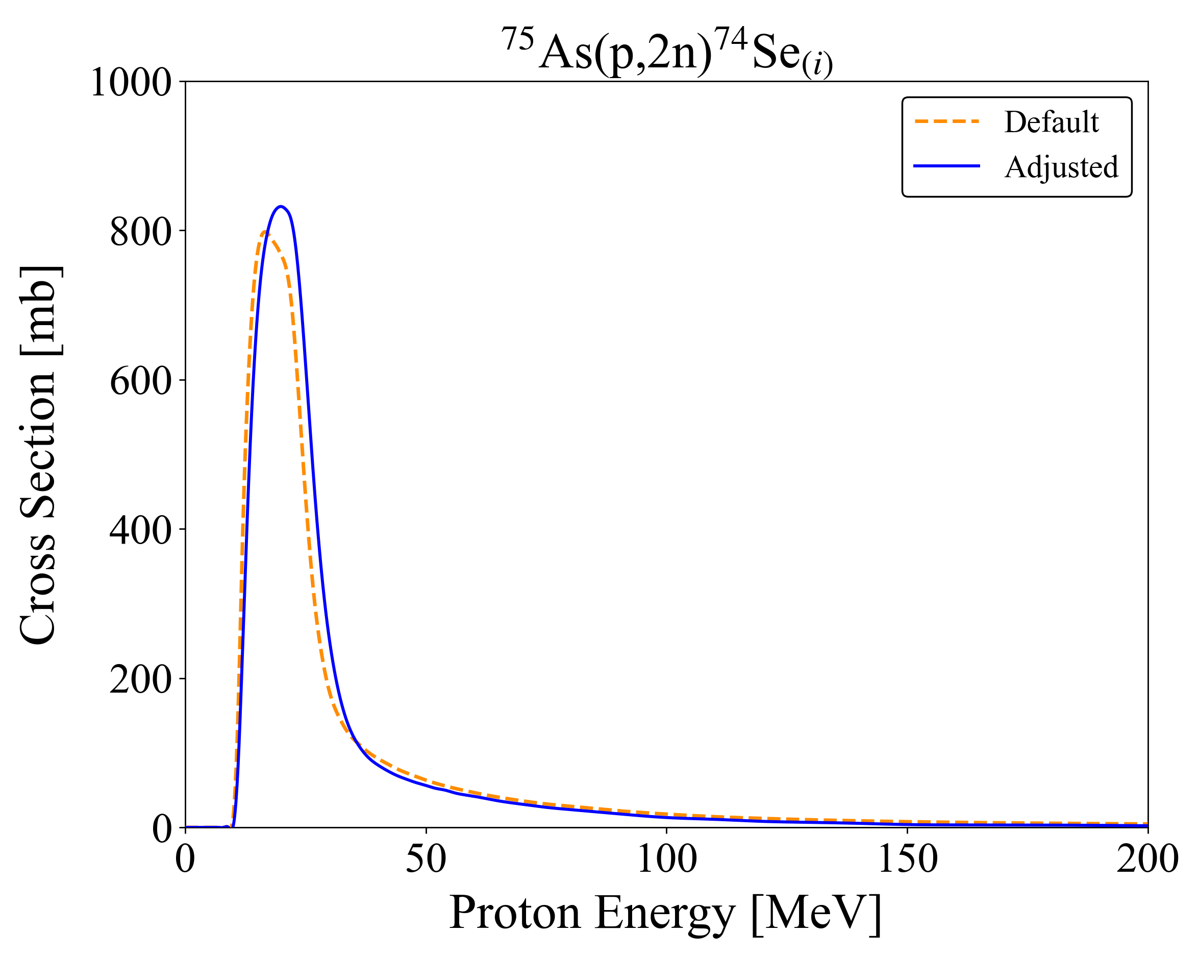
Figure 14: Performance check for behaviour of the adjusted fit in ⁷⁴Se, the largest unobserved channel from the fitting procedure.

IV.3 Parameter Adjustment Validation

As proposed in Fox et al. [21], validation for the suggested parameter changes can be performed by applying the adjusted fit to reaction channels not included in the initial adjustment sensitivity studies in Section IV.2. In this work, the validation channels ⁷⁵As(p,x)^72,70As, ^68,66Ge, ^72,66Ga, ^69m,65Zn, ^60,58,57,56Co help test for cumulative cross section effects and far-from-target modeling stability. ⁷⁵As(p,p3n)⁷²As is in fact independently measured here and meets many of the Fox et al. [21] criteria to be included as a residual product channel in the initial parameter optimization. However, since numerous neighboring competing Se and As channels to ⁷²As were already incorporated in Section IV.2, it became more worthwhile to save ⁷²As production as a significant channel for validation. Figure 15 demonstrates the adjusted fit behaviour in these validation channels, where consistently improved predictive power is seen.

It is also possible to further analyze the total non-elastic cross section predictions of the default and adjusted TALYS models, together with the TENDL evaluation (Figure 16). No experimental data points guide the ⁷⁵As(p,non) predictions, commensurate with the little prior published data for the residual product excitation functions as a whole. Even with the new data results of this paper, due to the unseen reaction products described in Section IV.2.1, it is not viable to derive any ⁷⁵As(p,non) data points from summing the measured cross sections. The adjusted (p,non) remains within the TENDL uncertainty band and its increase versus the default is defensible. Specifically, the adjusted (p,non) shares the same shape as the TENDL evaluation and the default prediction, which are based on global fits to other targets, and the increase in magnitude is validated based on changes seen in residual product channels such as ⁷³As in Figure 12d.

A $\chi^{2}_{tot}$ descriptive metric for comparing the default and adjusted TALYS fits across all presented excitation functions, following the formalism described in Fox et al. [21], is given in Table 6. Both weighting methodologies yield similar results and the adjusted fit is seen to outperform the default prediction. The $\chi^{2}_{tot}$ values are partially deflated relative to the ⁹³Nb(p,x) and ¹³⁹La(p,x) results in Fox et al. [21] on account of the heavy dependence on the arsenic cross section measurements provided in this work and their associated larger uncertainties (9.0–15%) stemming from the electroplating process. Consequently, the $\chi^{2}_{tot}$ results are more usefully viewed as a relative measure between fits rather than as absolute measure of goodness.

Table 6: Global $\chi^{2}$ metric describing goodness-of-fit for the default and adjusted TALYS calculations of ⁷⁵As(p,x). Low $\chi^{2}_{tot}$ values, and a case of $\chi^{2}_{tot}<1.0$, are seen as a function of large weights associated with the measured arsenic data.

Weighting Method	Default $\chi^{2}_{tot}$	Adjusted $\chi^{2}_{tot}$
Cumulative $\sigma$	2.55	0.58
Maximum $\sigma$	3.58	1.25

IV.4 Alternative Solutions and Limitations of the Fitting Procedure

The M2constant=0.80, M2limit=3.9, and M2shift=0.55 exciton model adjustments suggested in this paper match the trend of M2constant$<$1.0, M2limit$>$1.0, and M2shift$<$1.0 changes from the ⁹³Nb(p,x) and ¹³⁹La(p,x) fitting cases in Fox et al. [21]. As a result, the same systematic behaviour of a relative decrease for internal transition rates at intermediate proton energies ($E_{p}=20-60$ MeV) in the exciton model as derived from the Nb and La cases is seen in the As as well. These determined M2 pre-equilibrium adjustments therefore continue to be indicative of a needed global enhancement to the two-component exciton model.

However, due to the mathematical formulation of the exciton model in TALYS, which can be reviewed in detail in Koning and Duijvestijn [119], it has been found that in fact M2constant$<$1.0, M2limit$>$1.0, and M2shift$<$1.0 is not a required condition to generate the systematic behaviour. Instead, numerous sets of (M2constant,M2limit,M2shift) will reproduce the same decrease for internal transition rates and replicate the residual product cross section predictions of Section IV.2. For example, both (2.45, 0.7, 1.2) and (1.1, 2.85, 0.7) satisfy these conditions for the ⁷⁵As(p,x) fitting. Thus, the transition rate trend result from Fox et al. [21] is corroborated in this work but the M2 adjustment requirements to create this trend are revised. Moreover, since multiple triplets all predict the expected systematic behaviour for the reaction phase space transitioning between the Hauser-Feshbach and exciton models for nuclear reactions, it is not possible to conclude which triplet is more accurate without more diversified datasets such as particle emission spectra or prompt gamma yields by ⁷⁵As(p,x$\gamma$) [114].

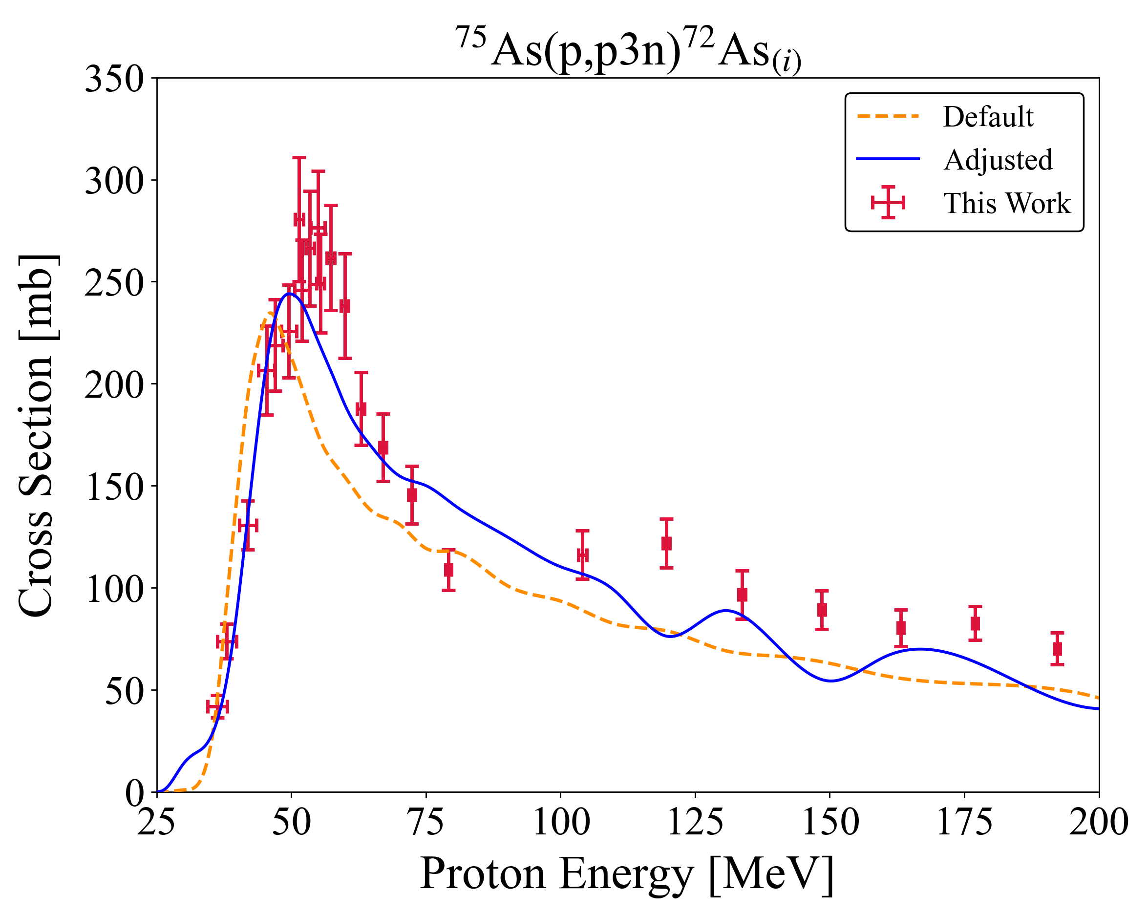
(a)

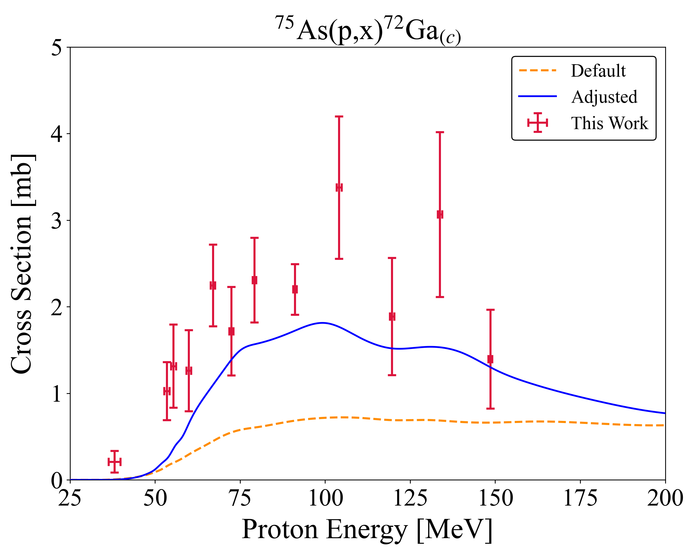
(b)

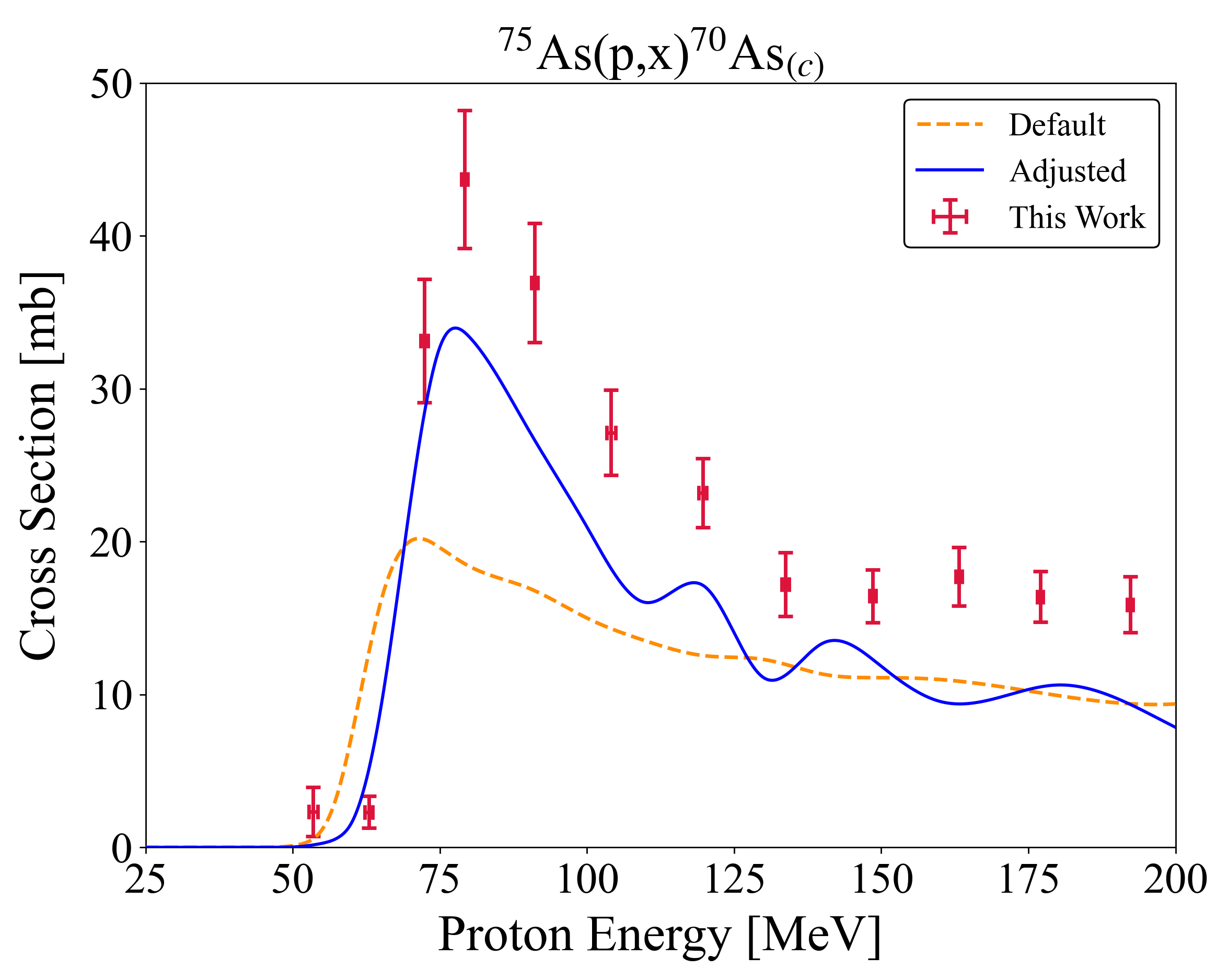
(c)

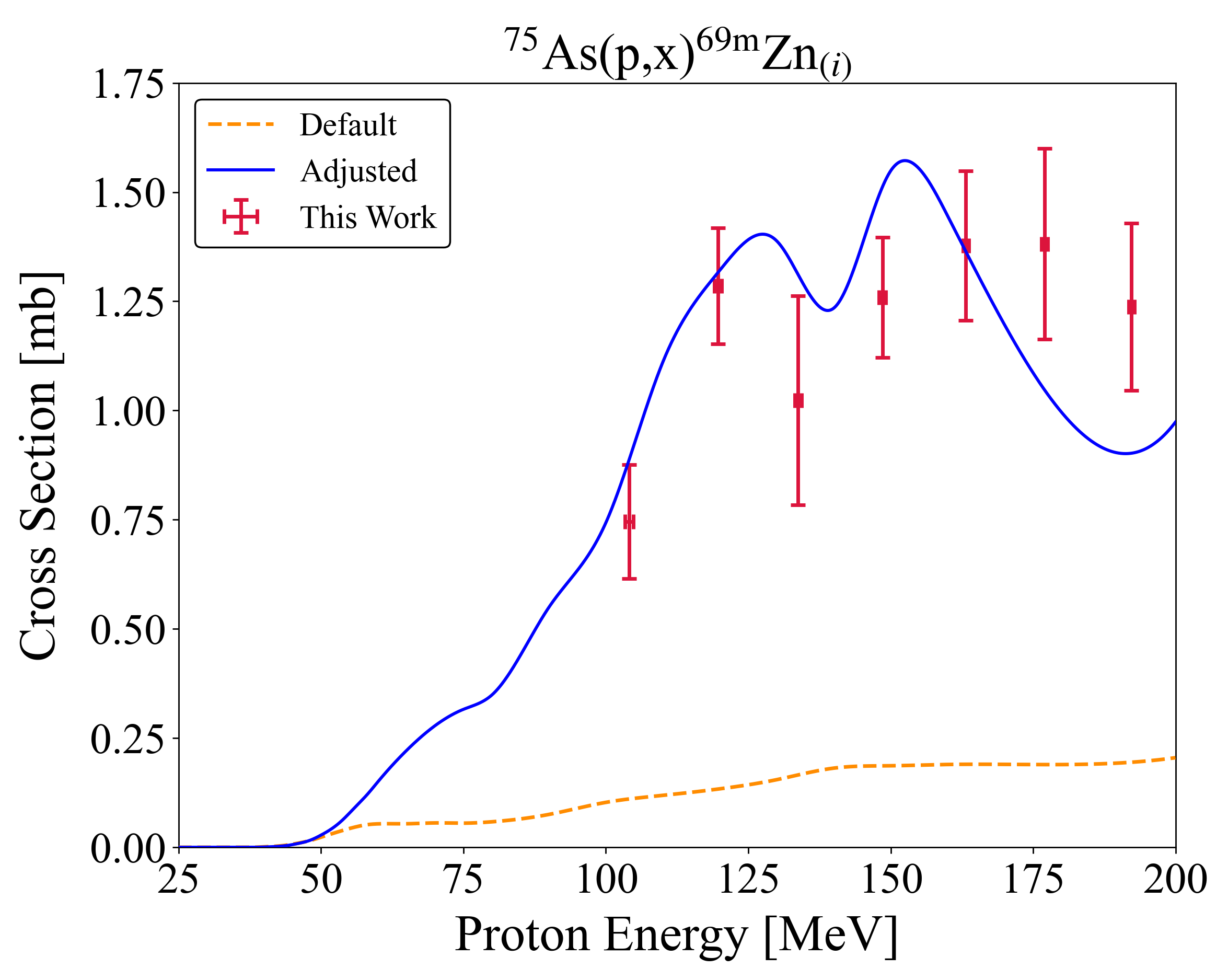
(d)

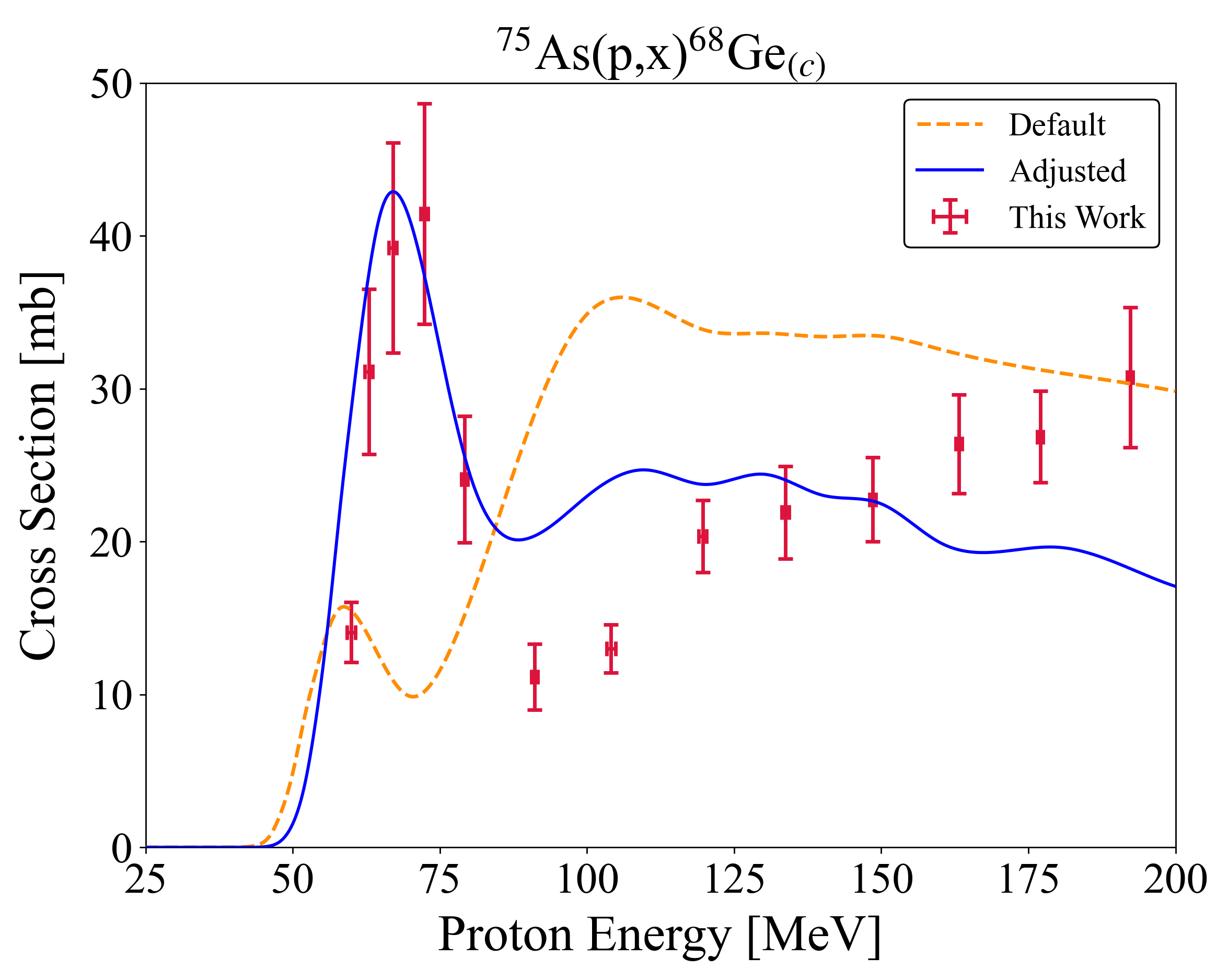
(e)

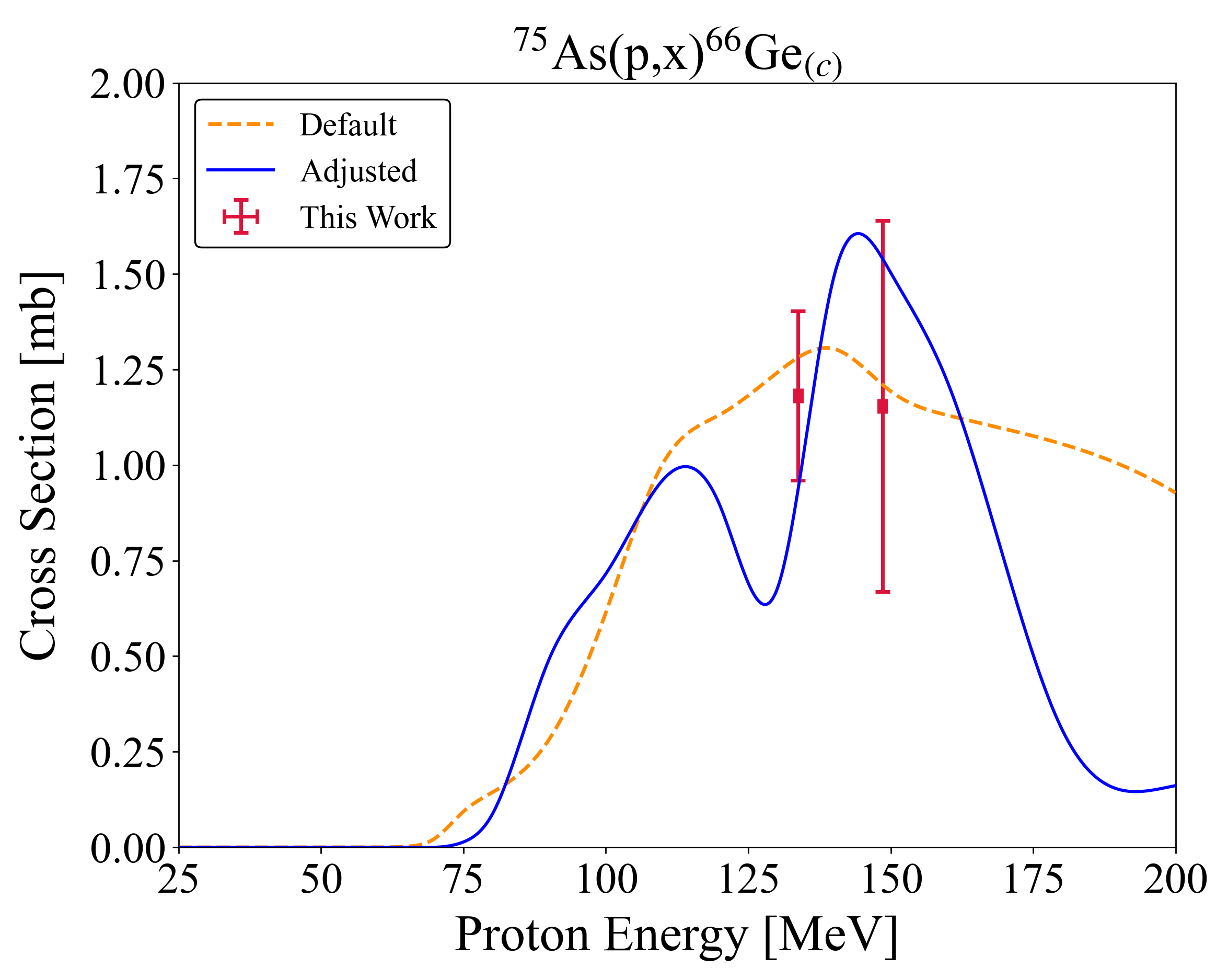
(f)

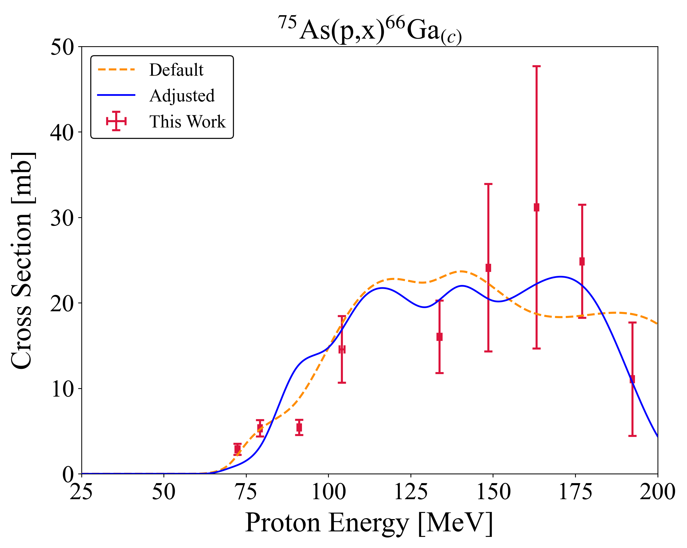
(g)

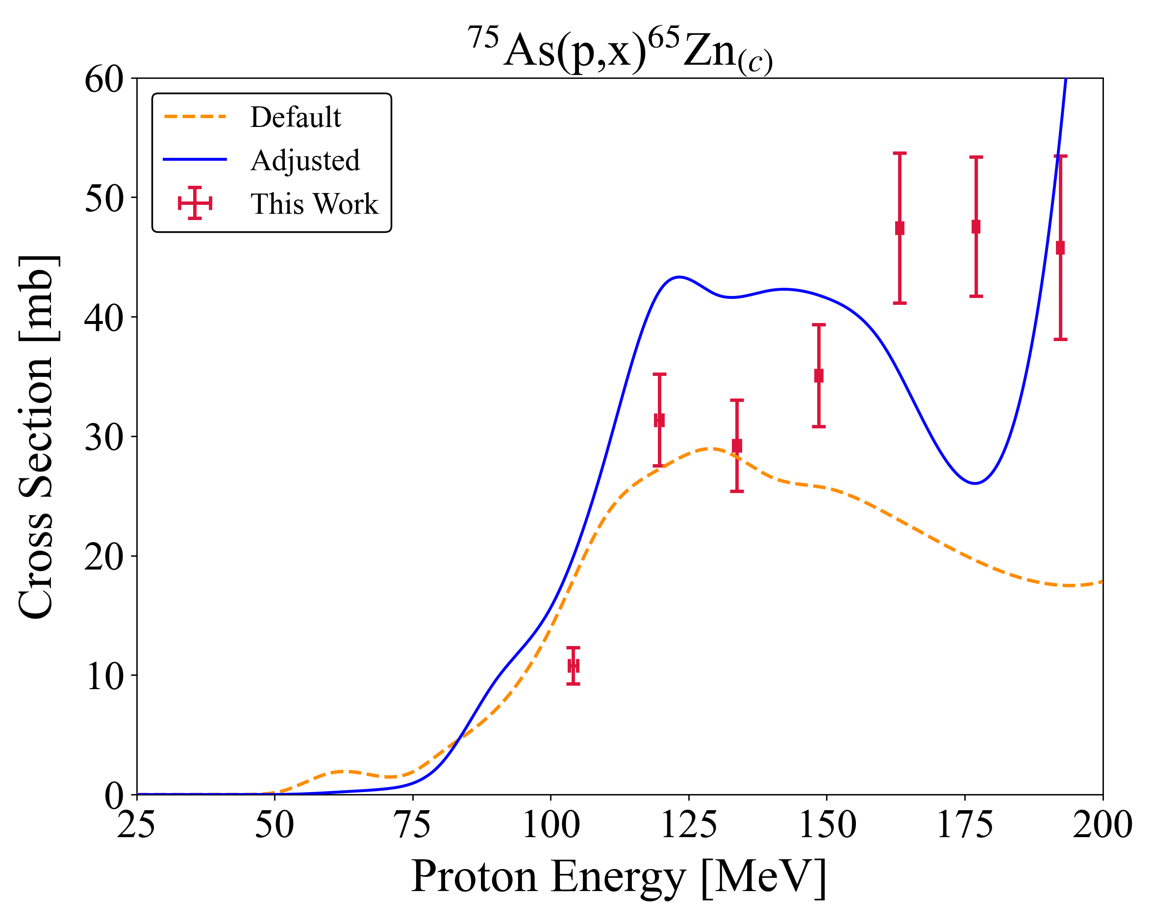
(h)

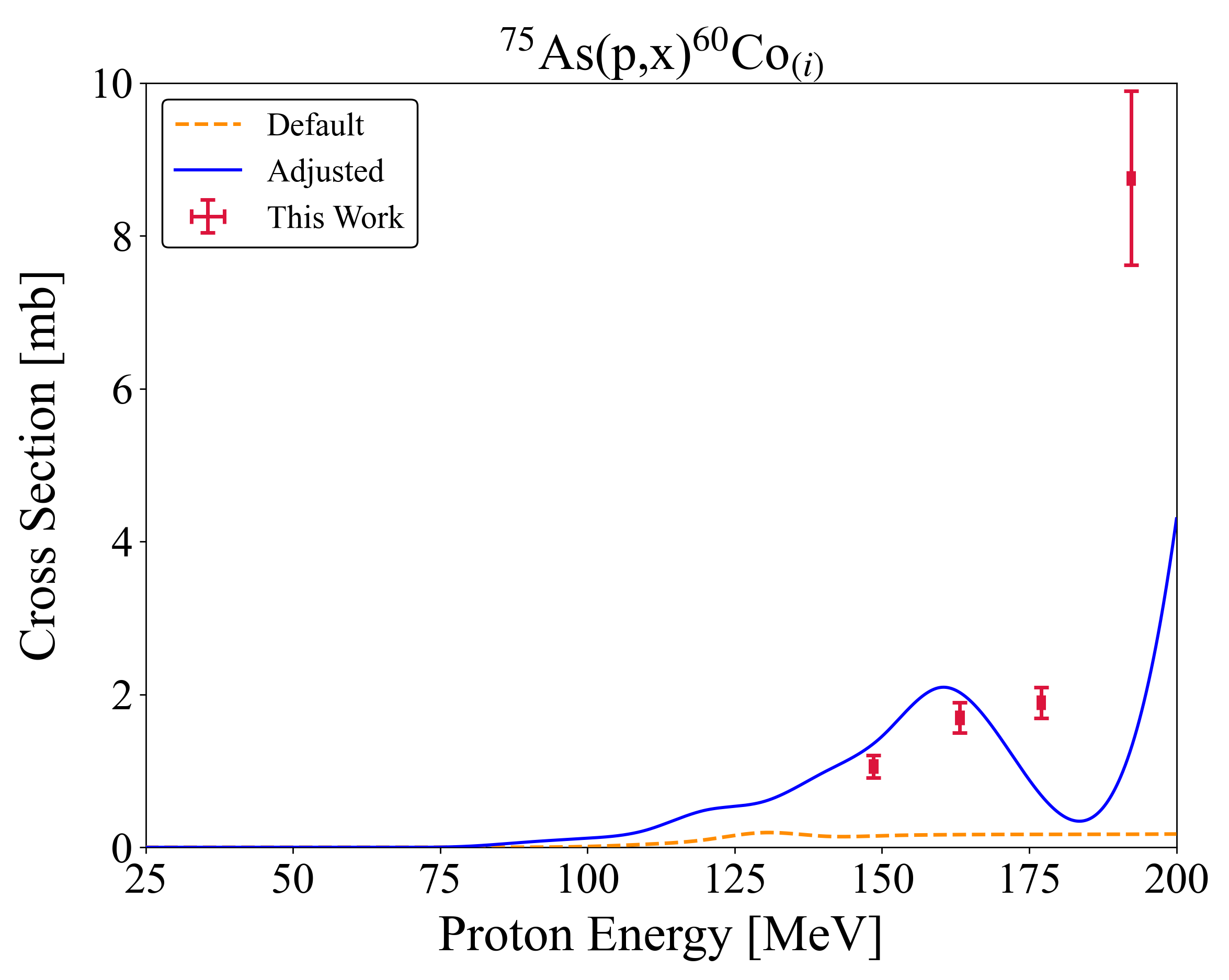
(i)

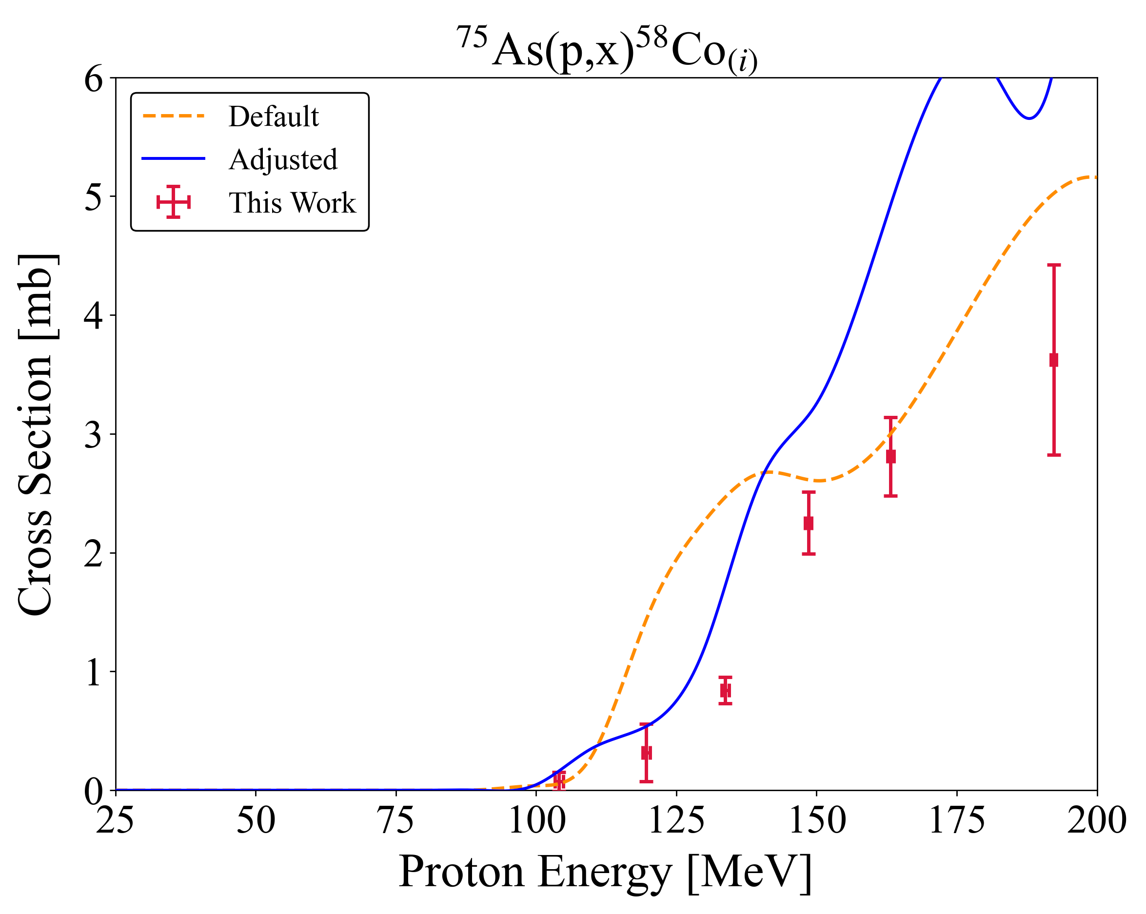
(j)

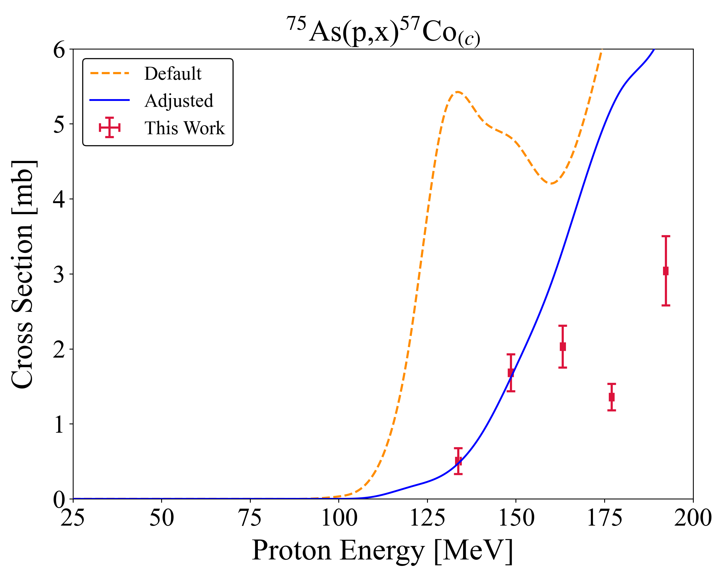
(k)

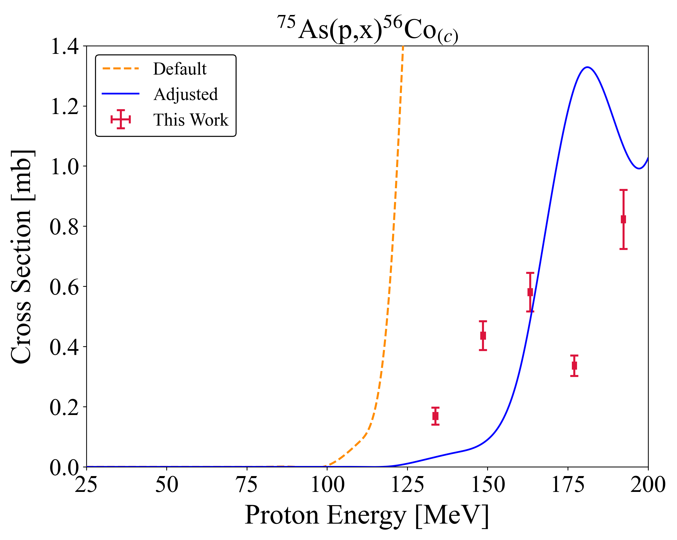
(l)

Figure 15: TALYS default and adjusted calculations extended to residual products not used in the parameter adjustment sensitivity studies.

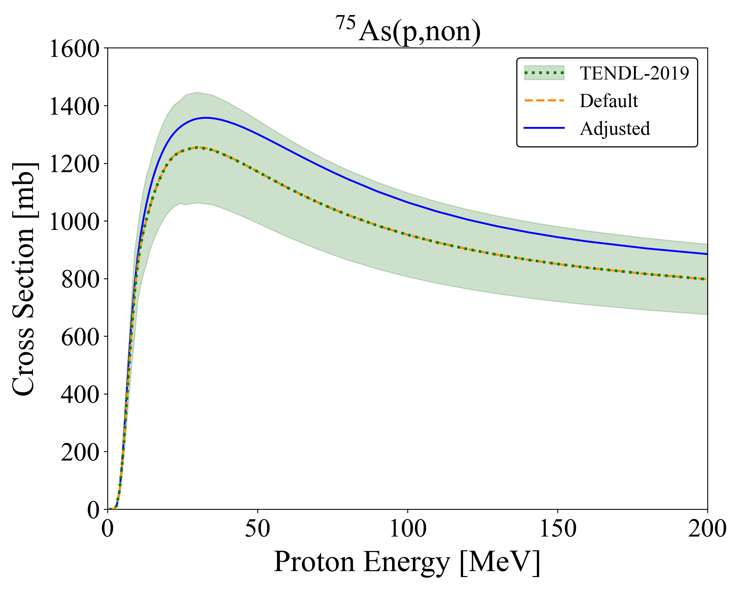
Figure 16: Comparison of evaluated and theoretical non-elastic cross sections. The filled error bands are associated with the TENDL data.

Indeed, this lack of diversified datasets is the overall limiting factor of the fitting procedure in its current state. The TALYS parameter space is extremely large and the effects of many parameters are hidden from high-energy residual product modeling. Furthermore, the secondary effects from pre-equilibrium, optical model, level density, and coupled-channels changes that are made cannot be deduced without other data types, which detracts from physical insights that can be made about the modeling physics in this work [120]. Prompt gamma data or emission spectra could act to concretely identify certain parameters as well as greatly reduce the remaining parameter space, all creating a more suitable and physical fit solution. Of course, these additional data types would themselves only be able to inform small portions of the incident energy range explored through stacked-target activation and would not be as useful without the abundance of residual product data. Clearly, continued high-energy reaction measurements of all types are both needed and complementary.

The size of the parameter space is a further limiting element since it leads to local minimum results for the fitting procedure, as was discussed for ⁶⁷Ga in this work. The implementation of automated searching and/or machine learning could likely mitigate this problem and would be in line with the sentiment of evaluators in the nuclear data community [121, 22].

Overall, these shortcomings emphasize that the thought process of the Fox et al. [21] fitting procedure is most relevant, and not every individual result – at this stage, because it principally builds evaluation considerations into nuclear data measurements. This is an important introductory step for an area where no formalism or data existed, as the evolution of this type of thought process better aligns data work and evaluations as a necessary path forward.

V Conclusions

This work furthers the Tri-laboratory Effort in Nuclear Data by reporting 55 sets of measured ⁷⁵As(p,x), ${}^{\textnormal{nat}}$Cu(p,x), and ${}^{\textnormal{nat}}$Ti(p,x) residual product cross sections between 35 and 200 MeV. The measured data most notably include the first cross section results for ⁷⁵As(p,x)⁶⁸Ge and the best characterized excitation function of ⁷⁵As(p,x)⁷²Se to-date, which are important for the production of the ⁶⁸Ge/⁶⁸Ga and ⁷²Se/⁷²As PET generator systems.

We have additionally continued to develop the Fox et al. [21] formalism for high-energy reaction modeling using the newly available measured ⁷⁵As(p,x) data. The modeling study in this paper corroborated the pre-equilibrium exciton model findings presented in Fox et al. [21] surrounding the transition between the compound and pre-equilibrium regions in TALYS. Furthermore, we provided an in-depth discussion on the limitations to modeling predictive power caused by the lack of level density knowledge for nuclei off of stability.

This paper merges experimental work and evaluation techniques for high-energy charged-particle isotope production in a continuance of the initial analysis of this kind. The consideration of these different aspects of the nuclear data pipeline together is a priority moving forwards that will benefit future data compilation, evaluation, and application.

The $\gamma$-ray spectra and all other raw data created during this research are openly available at http://doi.org/10.5281/zenodo.4648950 [122]. On publication, the experimentally determined cross sections will be uploaded to the EXFOR database.

Appendix A Additional LANL and BNL Target Stack Information

Details of the stacked-targets irradiated at LANL and BNL are given in Tables LABEL:LANLStack and 8, taken directly from Fox et al. [21].

Table 7: Target stack design for irradiation at IPF. The proton beam initially hits the stainless steel plate (SS-SN1) after passing through the upstream Inconel beam entrance window, a water cooling channel, and the target box aluminum window. The thickness and areal density measurements are prior to any application of the variance minimization techniques described in this work.

Target Layer	Thickness [$\mathrm{\SIUnitSymbolMicro}$m]	Areal Density [mg/cm2]	Areal Density Uncertainty [%]
SS-SN1 Profile Monitor	130.0	100.12	0.07
Al-SN1	27.33	7.51	0.21
Nb-SN1	25.75	23.08	0.12
As-SN1	4.27	2.45	8.2
Ti-SN1	25.00	11.265	1.0
Cu-SN1	24.33	19.04	0.13
Al Degrader 01	6307.0	1702.89	0.001
Al-SN2	26.67	7.58	0.32
Nb-SN2	24.75	22.67	0.08
As-SN2	4.30	2.46	8.3
Ti-SN2	25.00	11.265	1.0
Cu-SN2	24.00	18.90	0.36
Al Degrader 02	3185.5	860.09	0.02
Al-SN3	26.67	7.38	0.22
Nb-SN3	24.50	22.83	0.03
As-SN3	3.62	2.07	9.0
Ti-SN3	25.00	11.265	1.0
Cu-SN3	23.33	19.38	0.11
Al Degrader 03	2304.5	622.22	0.06
Al-SN4	28.00	7.34	0.18
Nb-SN4	25.50	22.57	0.16
As-SN4	3.54	2.03	9.2
Ti-SN4	25.00	11.265	1.0
Cu-SN4	24.67	19.24	0.11
Al Degrader 04	1581.3	426.94	0.04
Al-SN5	27.00	7.48	0.44
Nb-SN5	24.75	22.78	0.12
As-SN5	3.90	2.23	8.7
Ti-SN5	25.00	11.265	1.0
Cu-SN5	25.00	19.09	0.17
Al Degrader 05	1033.8	279.11	0.06
Al-SN6	28.67	7.44	0.25
Nb-SN6	25.25	22.80	0.08
As-SN6	3.11	1.78	10
Ti-SN6	25.00	11.265	1.0
Cu-SN6	24.33	19.50	0.16
Al Degrader 06	834.8	225.38	0.22
Al-SN7	28.33	7.56	0.15
Nb-SN7	25.50	22.62	0.06
As-SN7	2.79	1.59	9.2
Ti-SN7	25.00	11.265	1.0
Cu-SN7	23.67	18.79	0.04
Al Degrader 07	513.5	138.65	0.10
Al-SN8	27.67	7.56	0.10
Nb-SN8	25.50	22.95	0.45
As-SN8	2.20	1.26	9.0
Ti-SN8	25.00	11.265	1.0
Cu-SN8	24.00	19.06	0.23
Al Degrader 08	517.3	139.66	0.43
Al-SN9	27.00	7.47	0.36
Nb-SN9	25.00	22.53	0.24
As-SN9	2.57	1.47	9.9
Ti-SN9	25.00	11.265	1.0
Cu-SN9	26.33	19.19	0.12
Al Degrader 09	517.8	139.79	0.09
Al-SN10	28.00	7.41	0.17
Nb-SN10	24.75	22.82	0.02
As-SN10	1.94	1.11	10
Ti-SN10	25.00	11.265	1.0
Cu-SN10	25.67	18.87	0.18
SS-SN10 Profile Monitor	130.0	100.12	0.07

Table 8: Target stack design for irradiation at BLIP. The proton beam initially hits the stainless steel plate after passing through the upstream beam windows, water cooling channels, and target box aluminum window. The thickness and areal density measurements are prior to any application of the variance minimization techniques described in this work.

Target Layer	Thickness [$\mathrm{\SIUnitSymbolMicro}$m]	Areal Density [mg/cm2]	Areal Density Uncertainty [%]
SS Profile Monitor	120.2	95.16	0.58
Cu-SN1	26.00	22.34	0.10
Nb-SN1	25.75	22.75	0.25
As-SN1	1.89	1.08	9.9
Ti-SN1	25.00	11.265	1.0
Cu Degrader 01	5261.1	4708.07	0.02
Cu-SN2	26.75	22.41	0.11
Nb-SN2	24.75	22.91	0.19
As-SN2	2.94	1.68	9.0
Ti-SN2	25.00	11.265	1.0
Cu Degrader 02	4490.7	4018.99	0.04
Cu-SN3	26.50	22.26	0.05
Nb-SN3	24.00	22.67	0.31
As-SN3	3.06	1.75	10
Ti-SN3	25.00	11.265	1.0
Cu Degrader 03	4501.8	4028.84	0.03
Cu-SN4	26.00	22.29	0.15
Nb-SN4	24.75	22.70	0.23
As-SN4	4.85	2.78	9.9
Ti-SN4	25.00	11.265	1.0
Cu Degrader 04	4243.9	3797.96	0.03
Cu-SN5	25.50	22.35	0.04
Nb-SN5	25.00	22.54	0.12
As-SN5	7.26	4.15	12
Ti-SN5	25.00	11.265	1.0
Cu Degrader 05	3733.8	3341.56	0.03
Cu-SN6	26.25	22.34	0.08
Nb-SN6	25.00	22.36	0.24
As-SN6	4.93	2.82	9.0
Ti-SN6	25.00	11.265	1.0
Cu Degrader 06	3783.0	3385.41	0.04
Cu-SN7	25.75	22.26	0.09
Nb-SN7	25.75	22.62	0.10
As-SN7	12.62	7.22	9.3
Ti-SN7	25.00	11.265	1.0

Appendix B Proton Current Variance Minimization

The applied variance minimization technique for the LBNL irradiation is summarized in Figure 18. A 4.23% increase to stopping power in simulations, implemented through an equivalent increase to degraders’ effective density in the stack, best reduced proton fluence measurement disagreements between different monitor channels in each energy compartment. This is in general agreement with results of past stacked-target work that have shown a needed modest positive enhancement to the stopping power of +2–5% [23, 25, 24].

The associated proton flux spectrum propagating through the stack, after variance minimization, is provided in Figure 18. The energy assignments for each foil in a stack are then the flux-averaged energies from the spectrum with uncertainties per foil taken as the full width at half maximum.

This same calculation methodology can be reviewed in detail for the LANL and BNL stacks in Fox et al. [21]

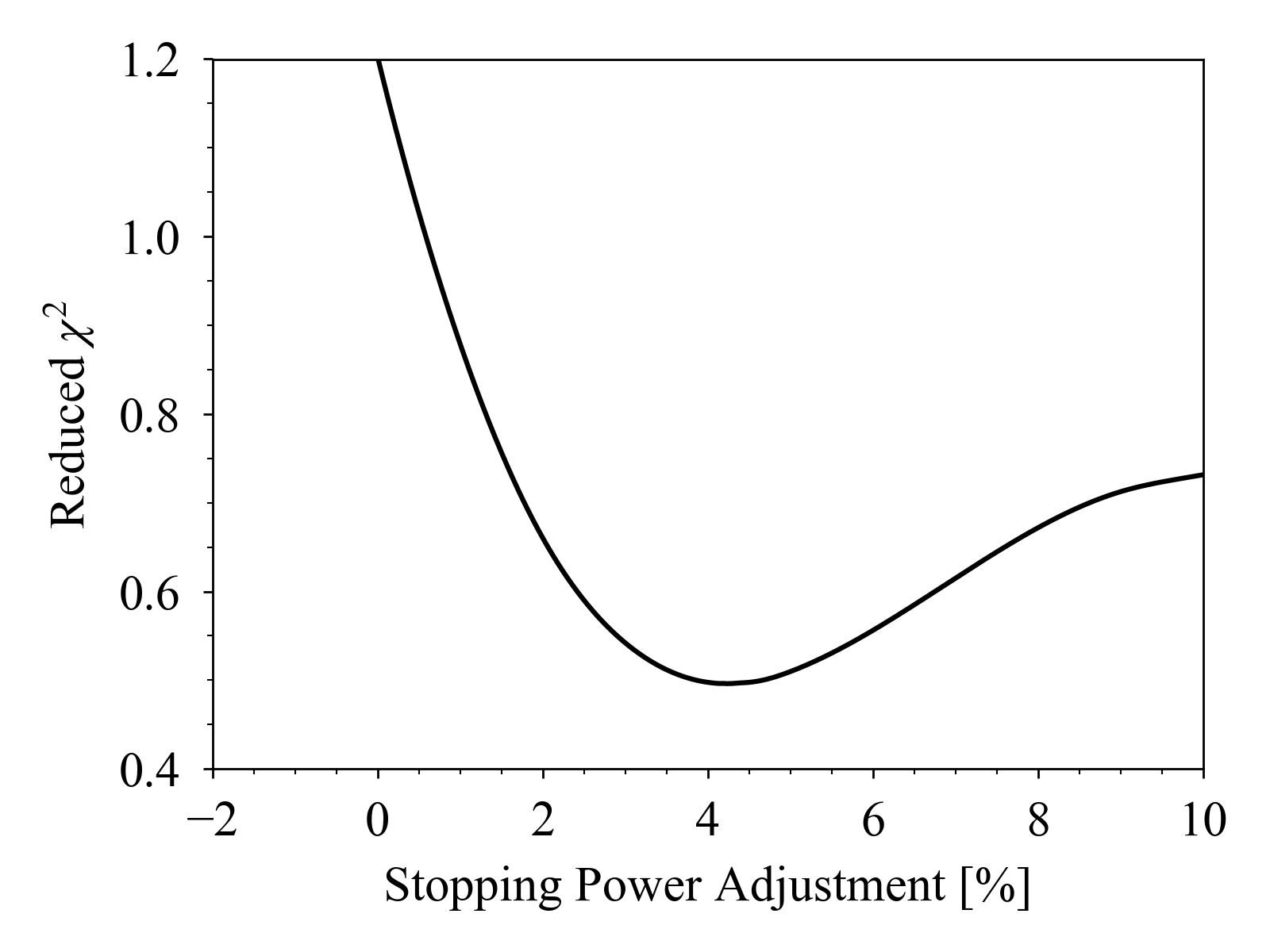
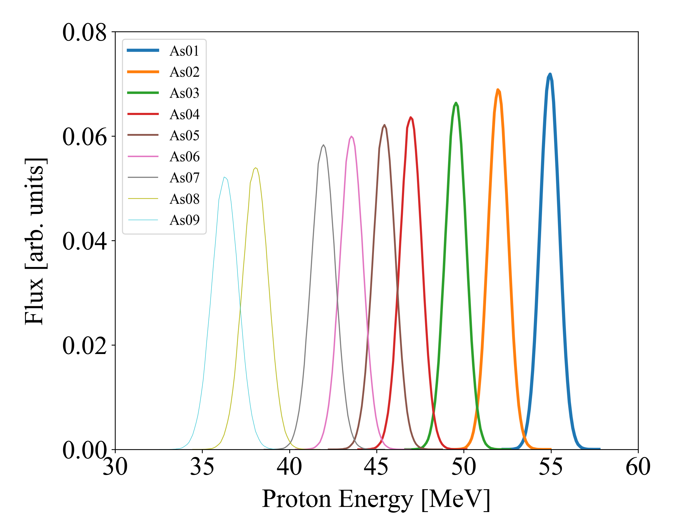
Figure 17: Result of $\chi^{2}$ optimization used in the variance minimization of the global linear fit to the monitor fluence data, indicating a required increase to stopping power in transport simulations.

Figure 18: Visualization of the calculated proton energy spectrum for each arsenic target in the LBNL stack, following variance minimization.

Appendix C Measured Excitation Functions

Plots of extracted cross sections in this work are given (Figures 21–69) with reference to existing literature data, TENDL-2019, and reaction modeling codes TALYS-1.9, EMPIRE-3.2.3, CoH-3.5.3, and ALICE-20 using default parameters [7, 39, 40, 41, 42, 43, 44, 45, 46, 47, 48, 49, 50, 51, 52, 53, 54, 55, 56, 57, 58, 59, 60, 61, 25, 23, 62, 63, 64, 65, 66, 67, 68, 24, 69, 70, 71, 72, 73, 74, 75, 76, 77, 78, 79, 33]. Subscripts $(i)$ and $(c)$ in figure titles indicate independent and cumulative cross sections, respectively.

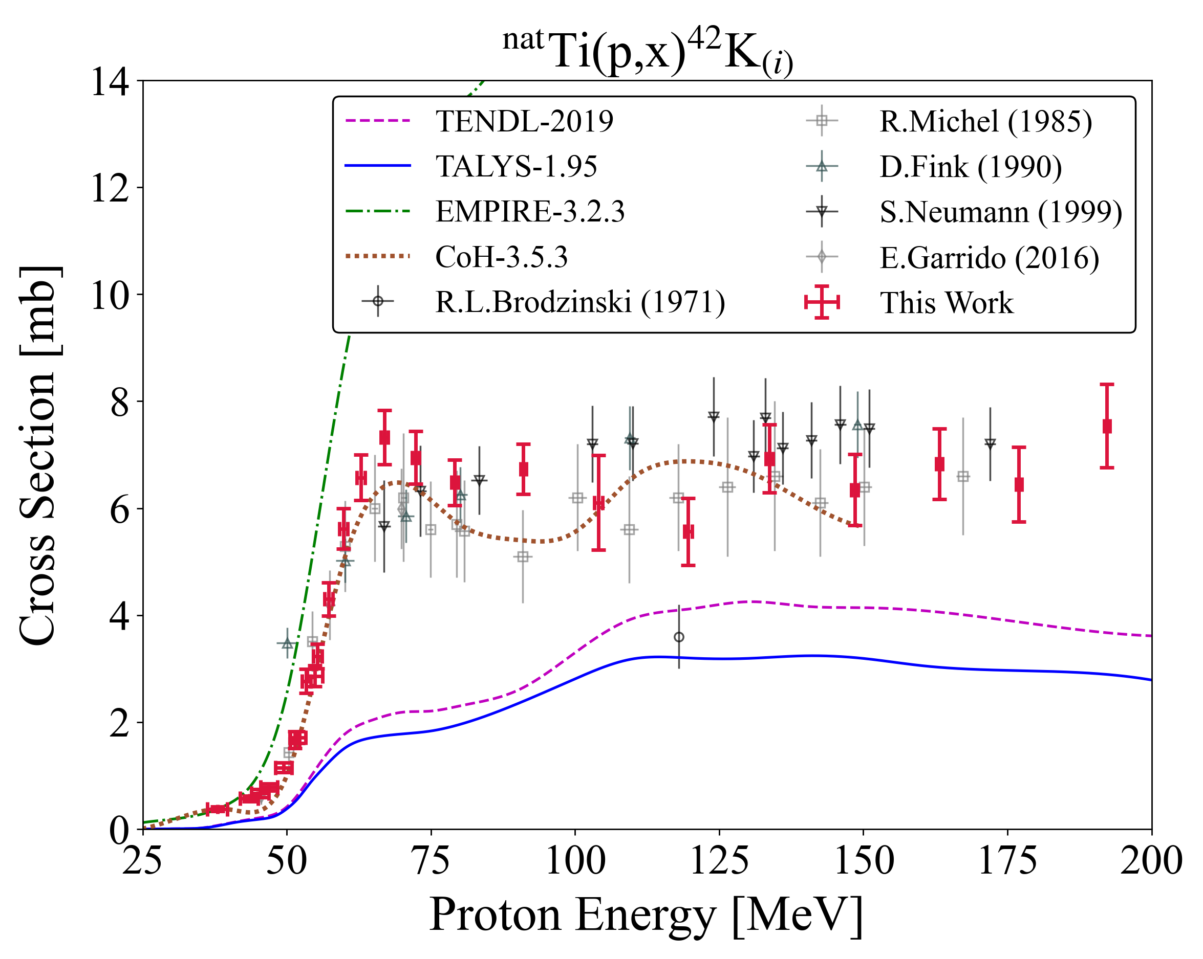
Figure 19: Experimental and theoretical cross sections for ⁴²K production.

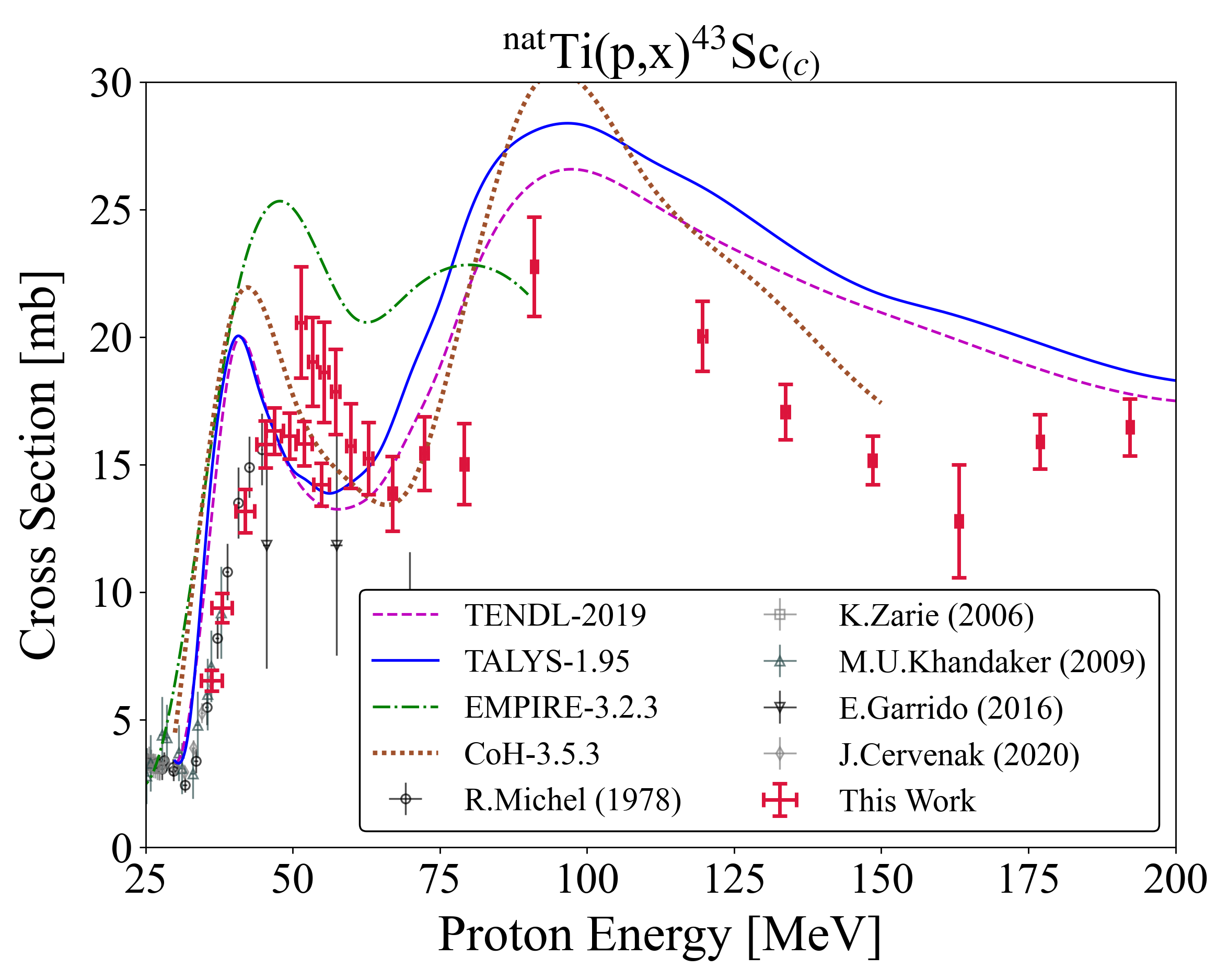
Figure 20: Experimental and theoretical cross sections for ⁴³K production.

Figure 21: Experimental and theoretical cross sections for ⁴³Sc production.

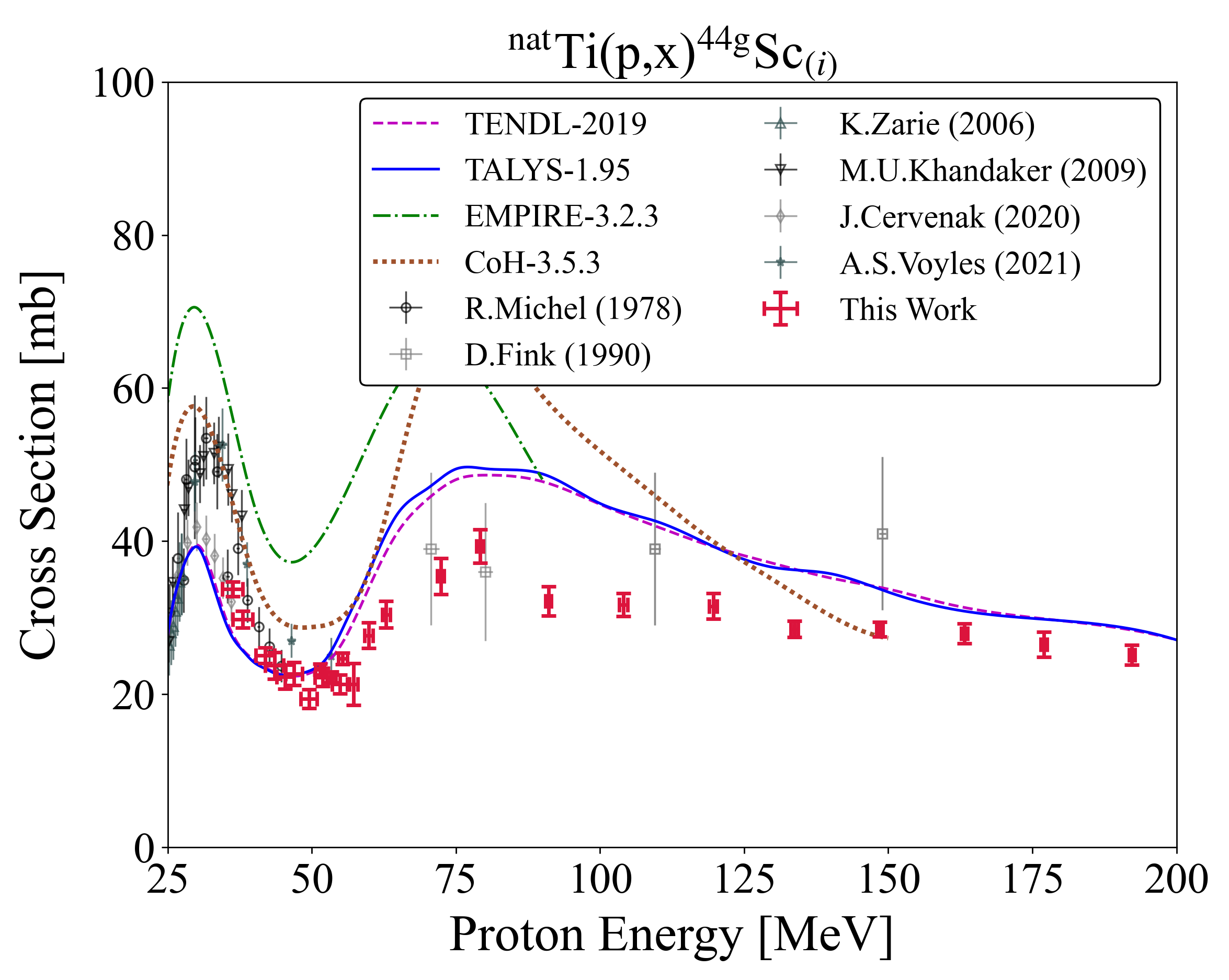
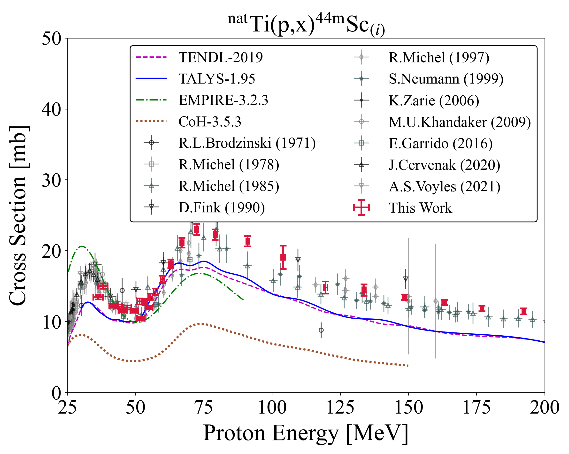
Figure 22: Experimental and theoretical cross sections for ${}^{\textnormal{44g}}$Sc production.

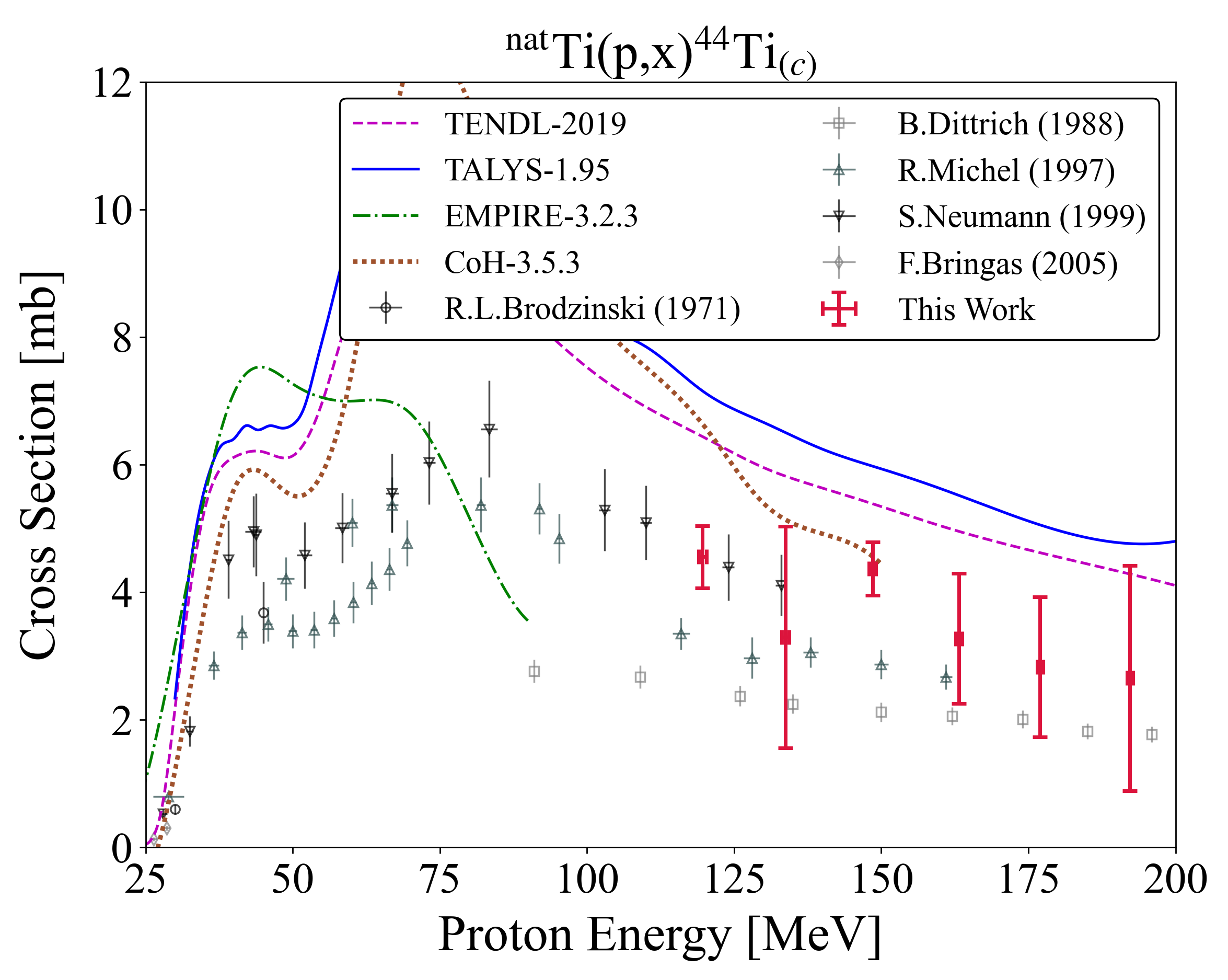
Figure 23: Experimental and theoretical cross sections for ${}^{\textnormal{44m}}$Sc production.

Figure 24: Experimental and theoretical cross sections for ⁴⁴Ti production.

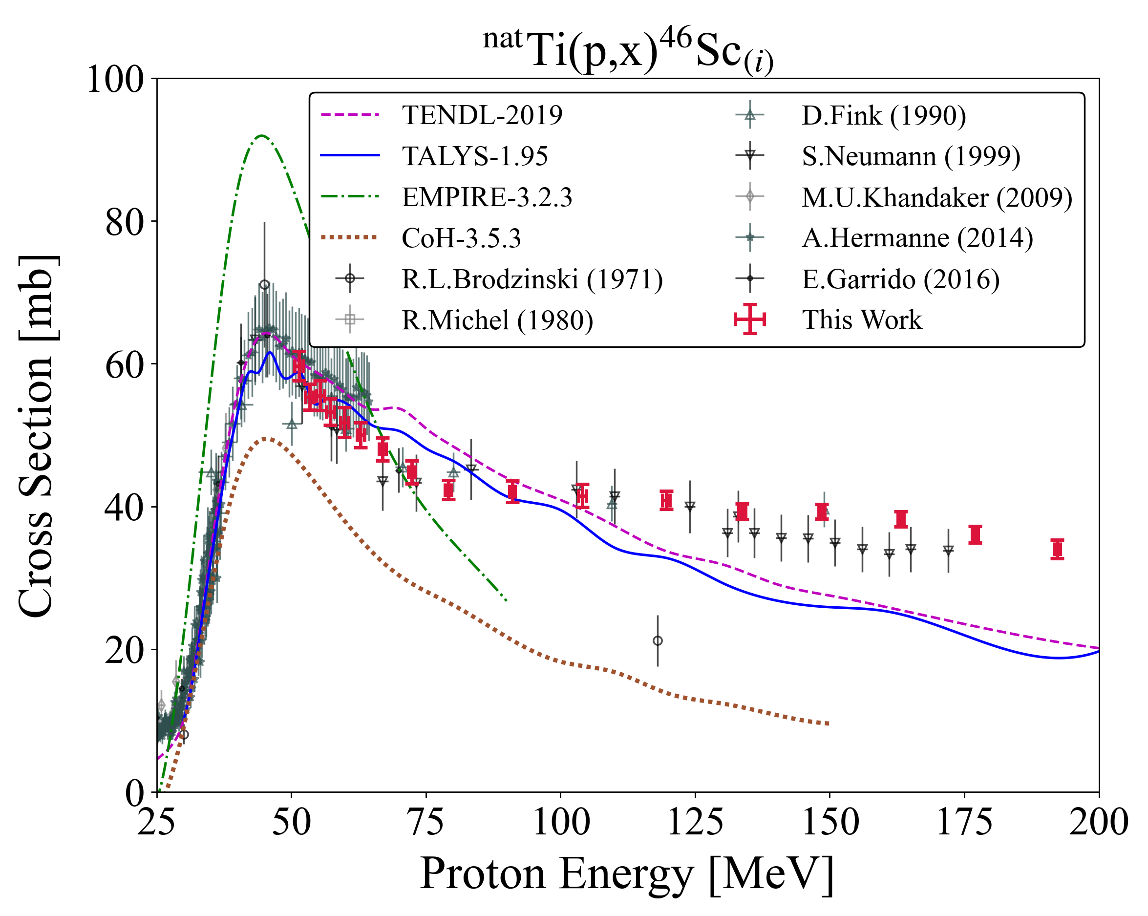
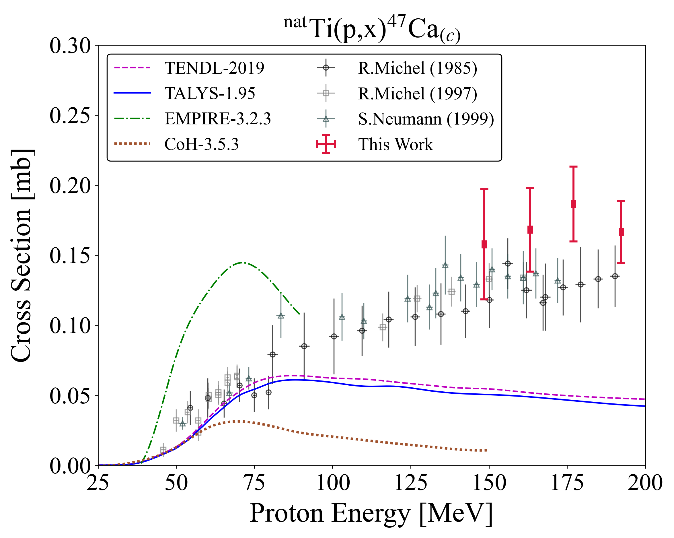
Figure 25: Experimental and theoretical cross sections for ⁴⁶Sc production.

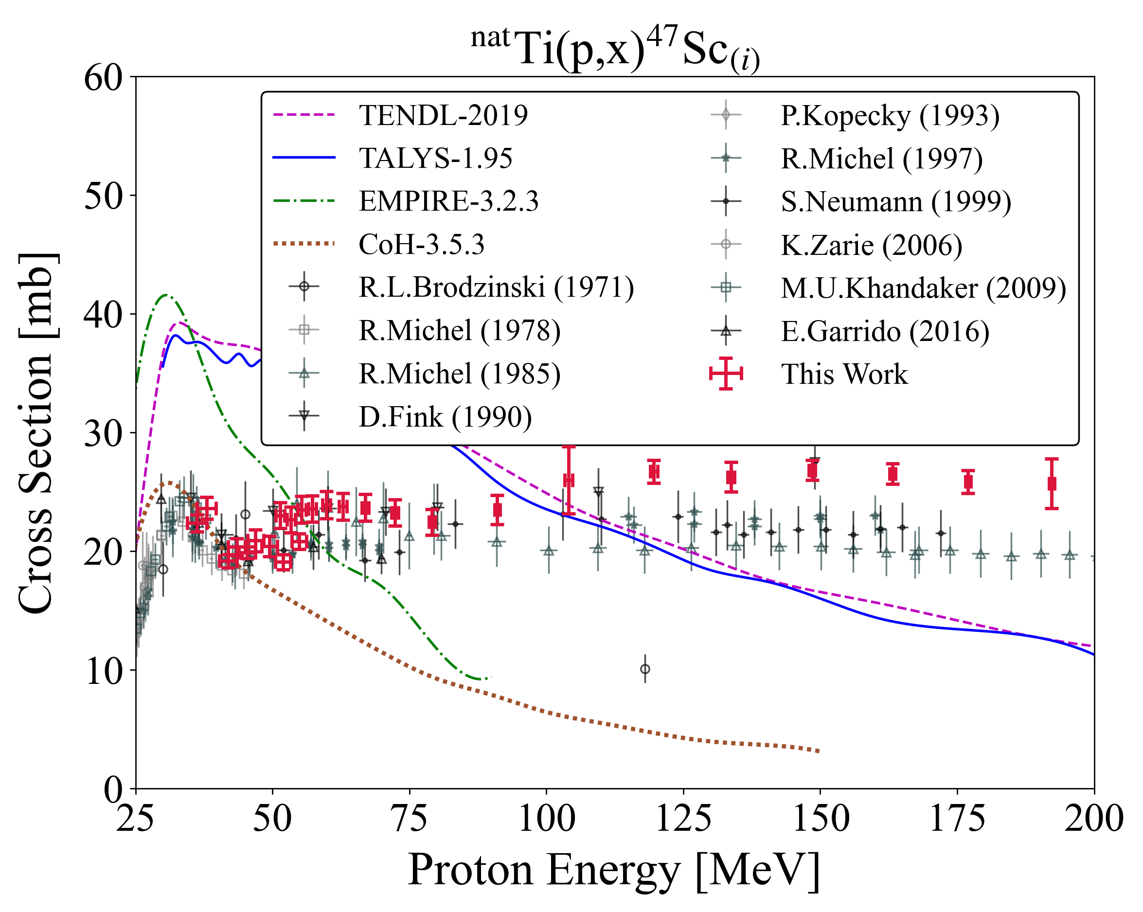
Figure 26: Experimental and theoretical cross sections for ⁴⁷Ca production.

Figure 27: Experimental and theoretical cross sections for ⁴⁷Sc production.

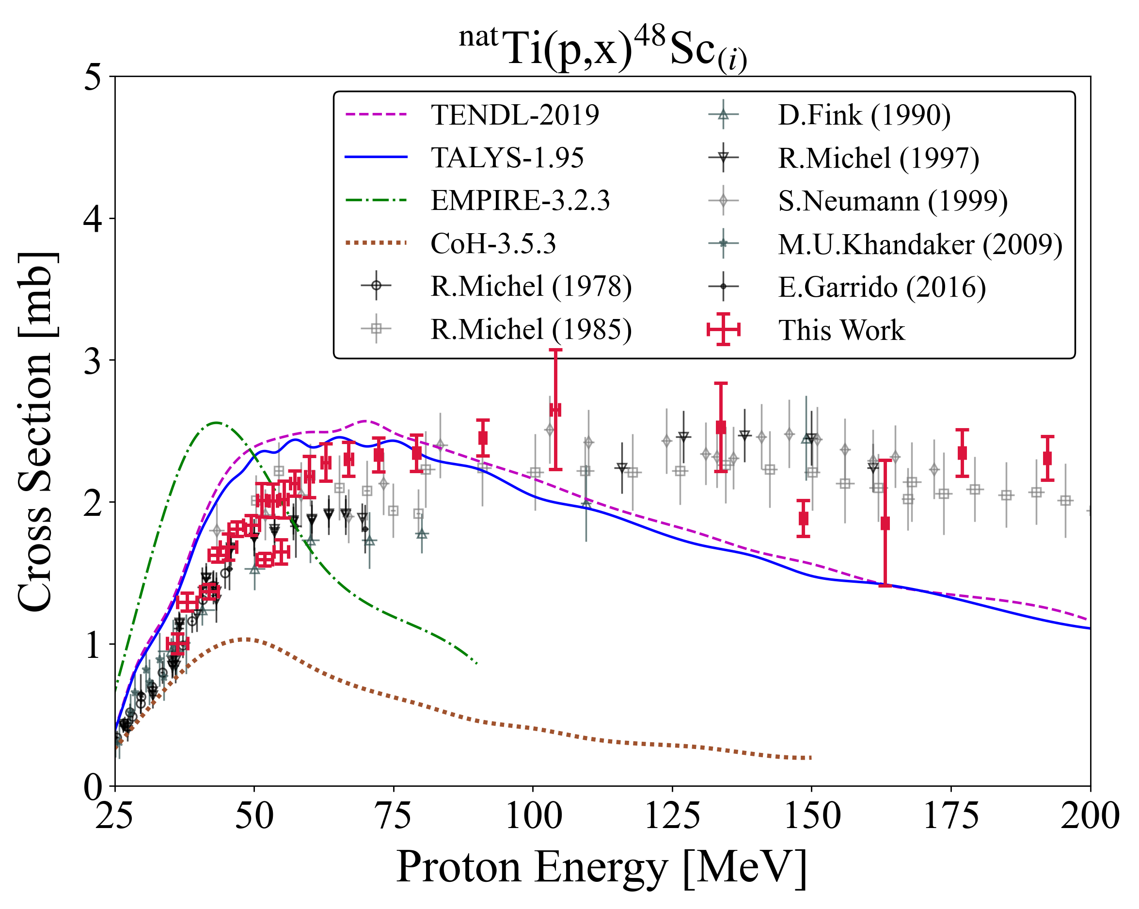
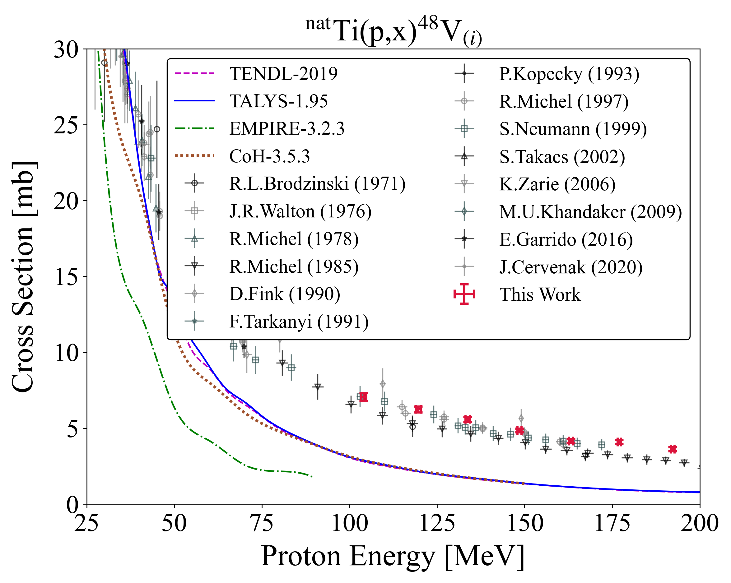
Figure 28: Experimental and theoretical cross sections for ⁴⁸Sc production.

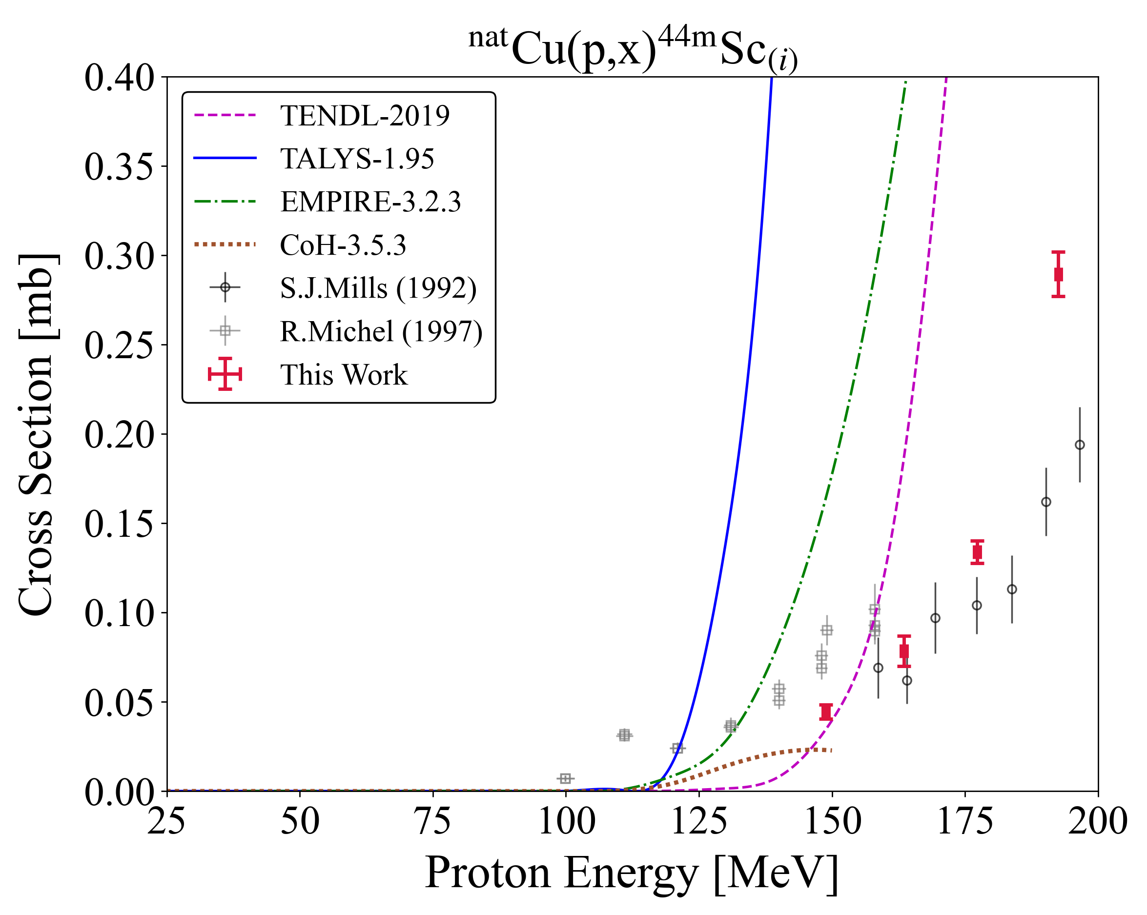
Figure 29: Experimental and theoretical cross sections for ⁴⁸V production.

Figure 30: Experimental and theoretical cross sections for ${}^{\textnormal{44m}}$Sc production.

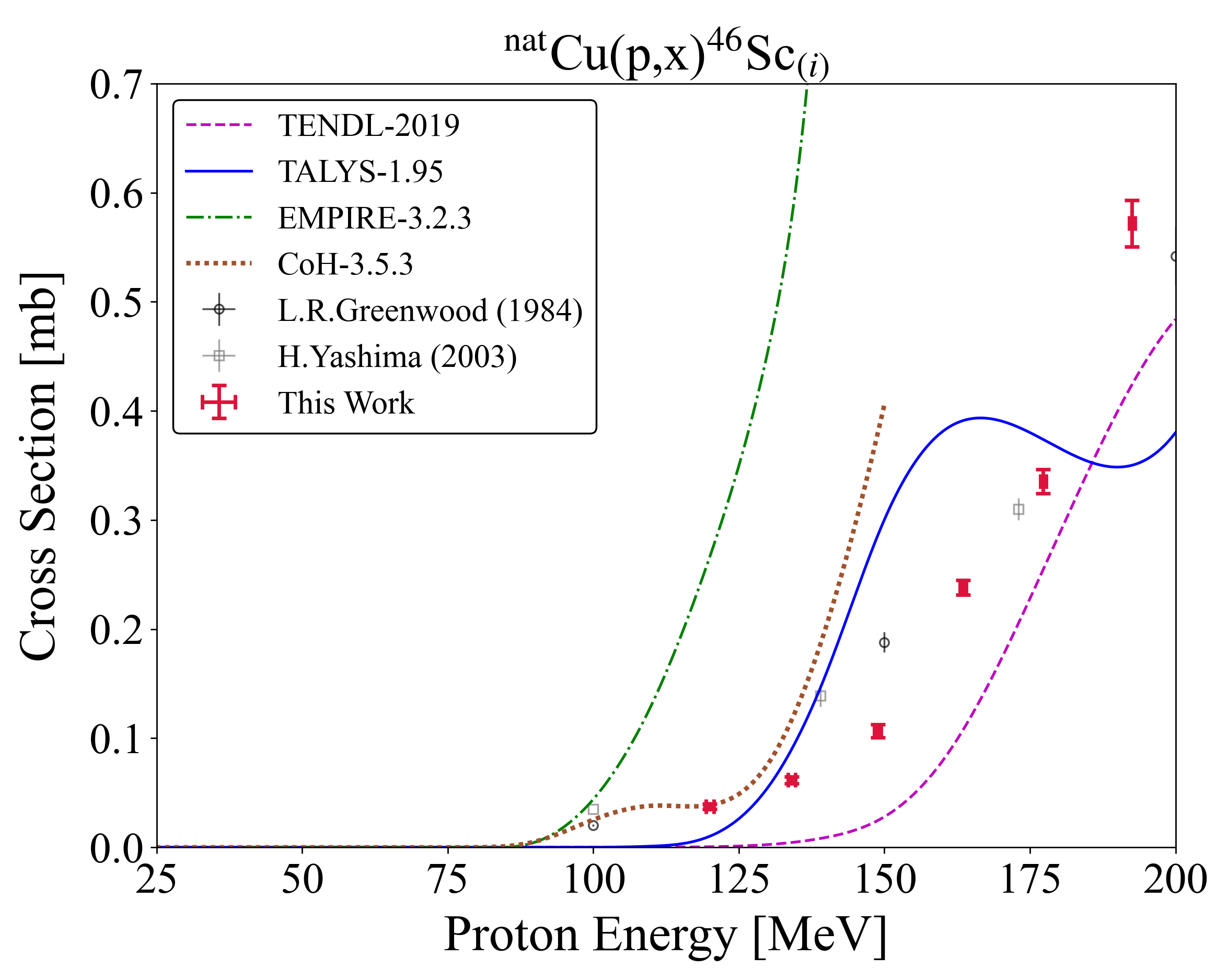
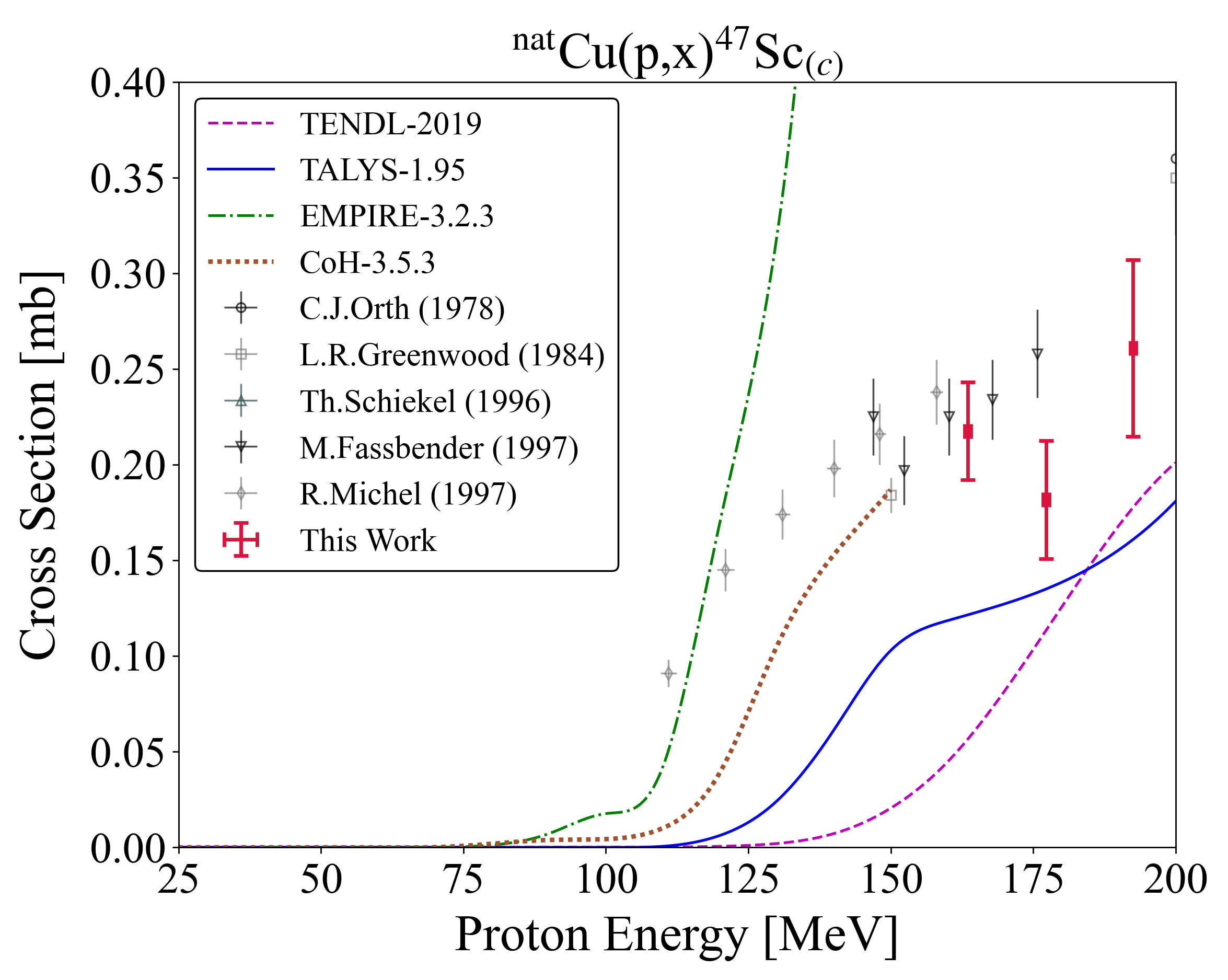
Figure 31: Experimental and theoretical cross sections for ⁴⁶Sc production.

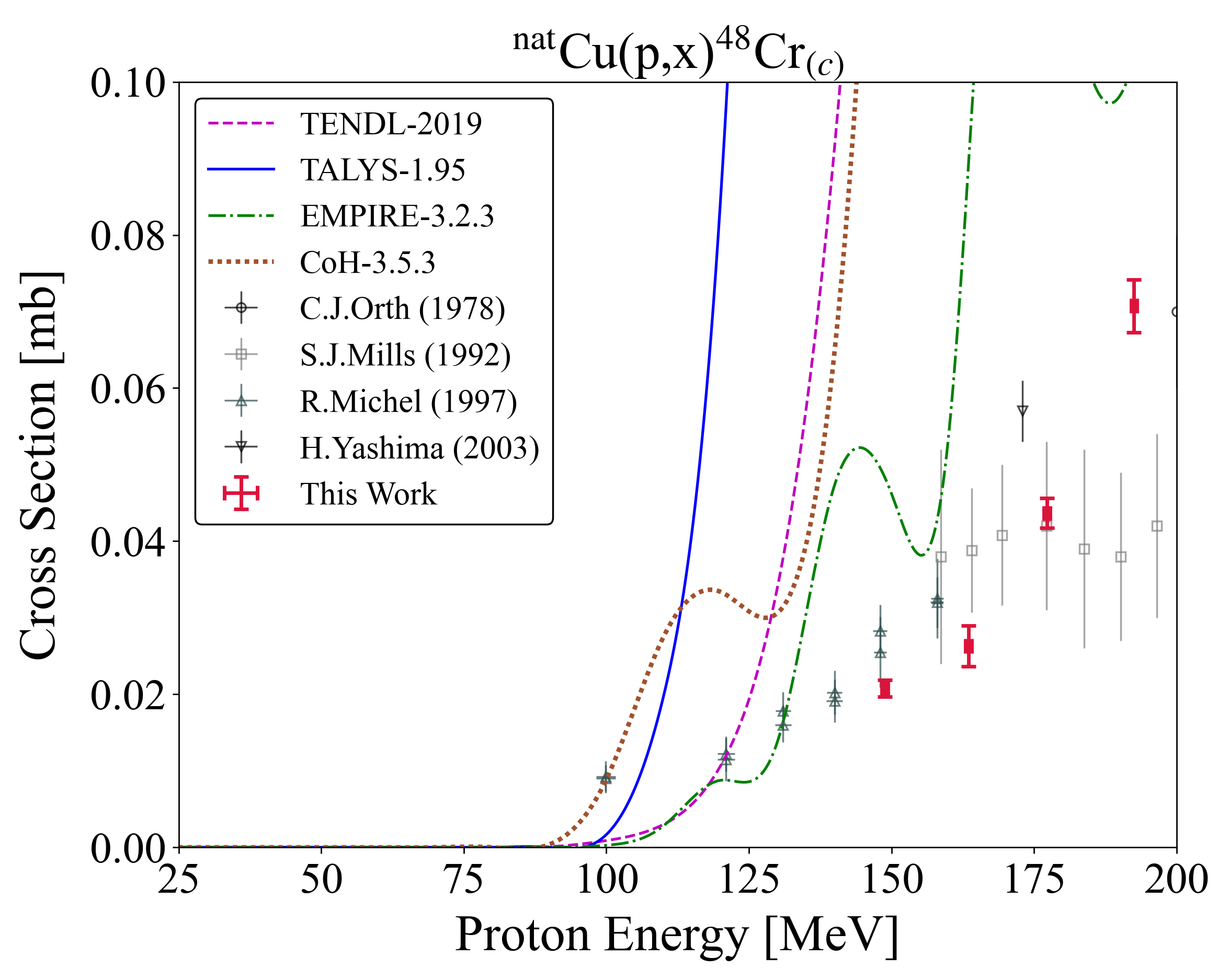
Figure 32: Experimental and theoretical cross sections for ⁴⁷Sc production.

Figure 33: Experimental and theoretical cross sections for ⁴⁸Cr production.

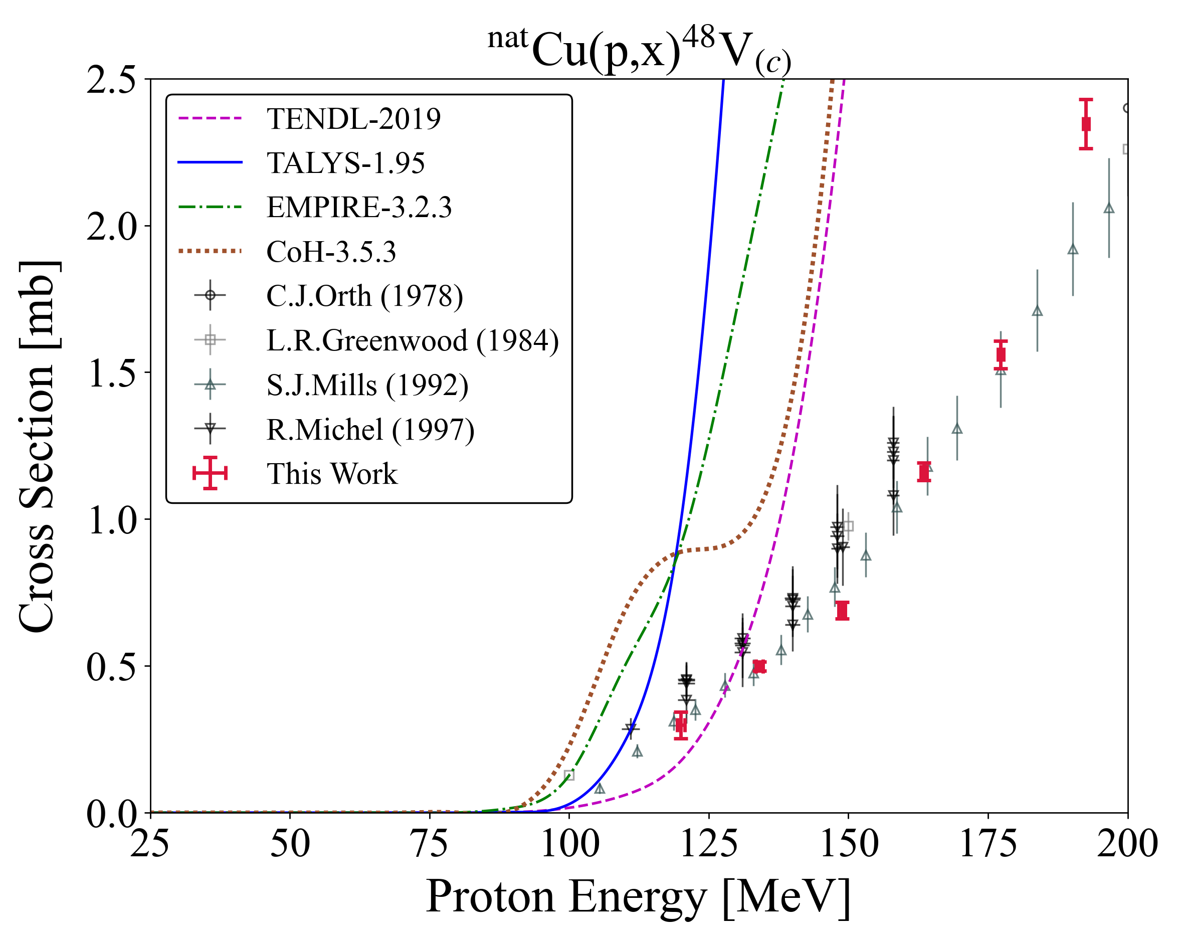
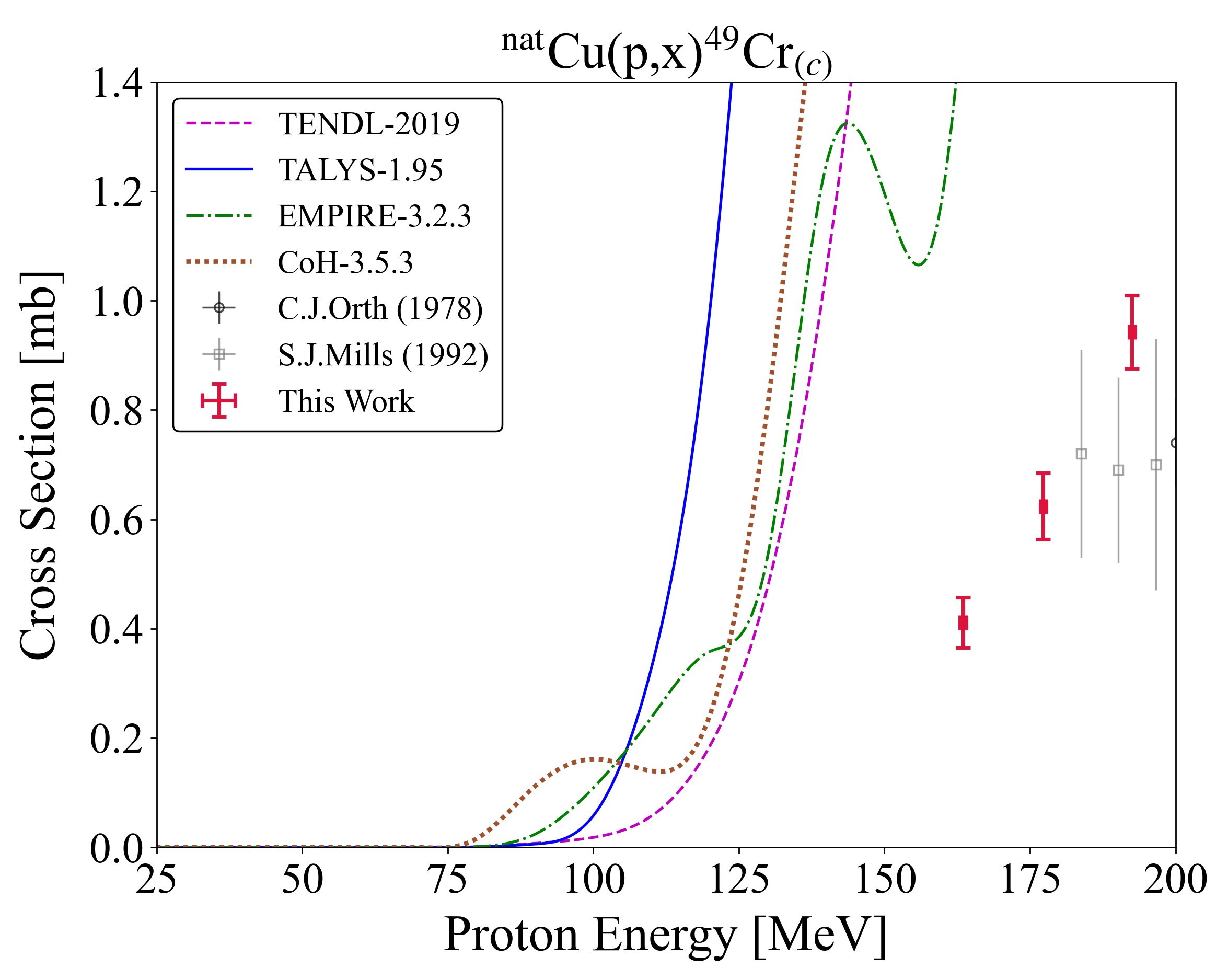
Figure 34: Experimental and theoretical cross sections for ⁴⁸V production.

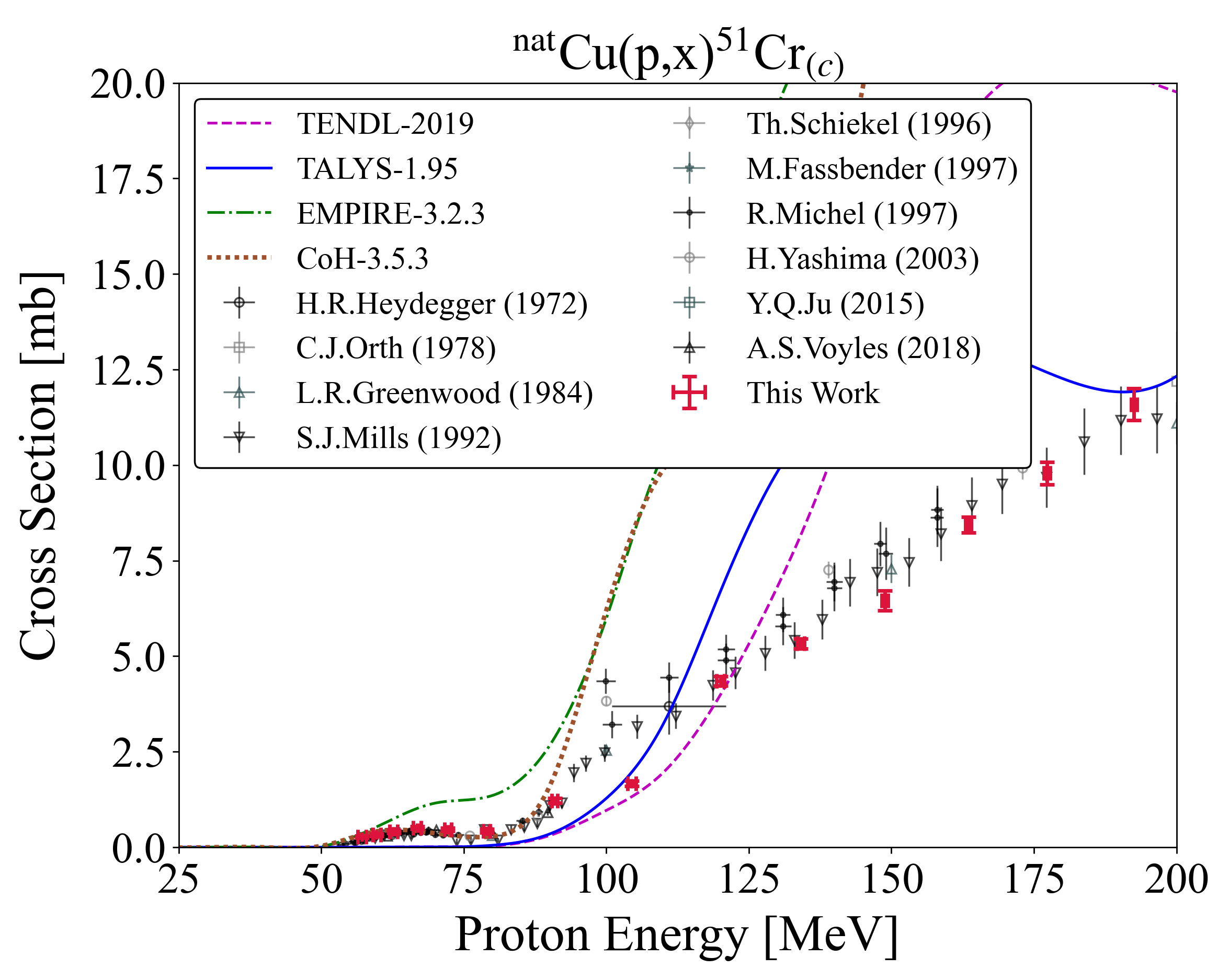
Figure 35: Experimental and theoretical cross sections for ⁴⁹Cr production.

Figure 36: Experimental and theoretical cross sections for ⁵¹Cr production.

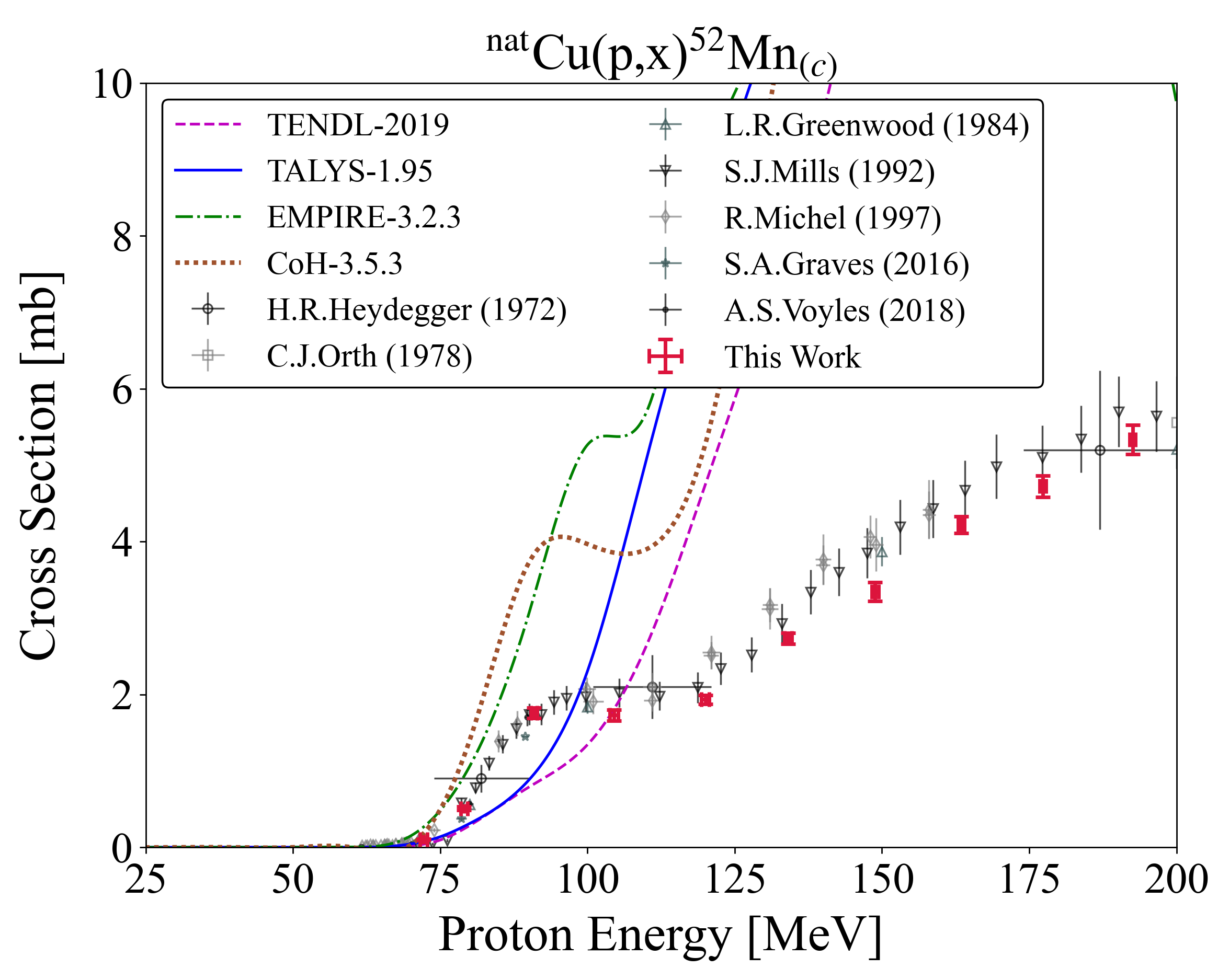
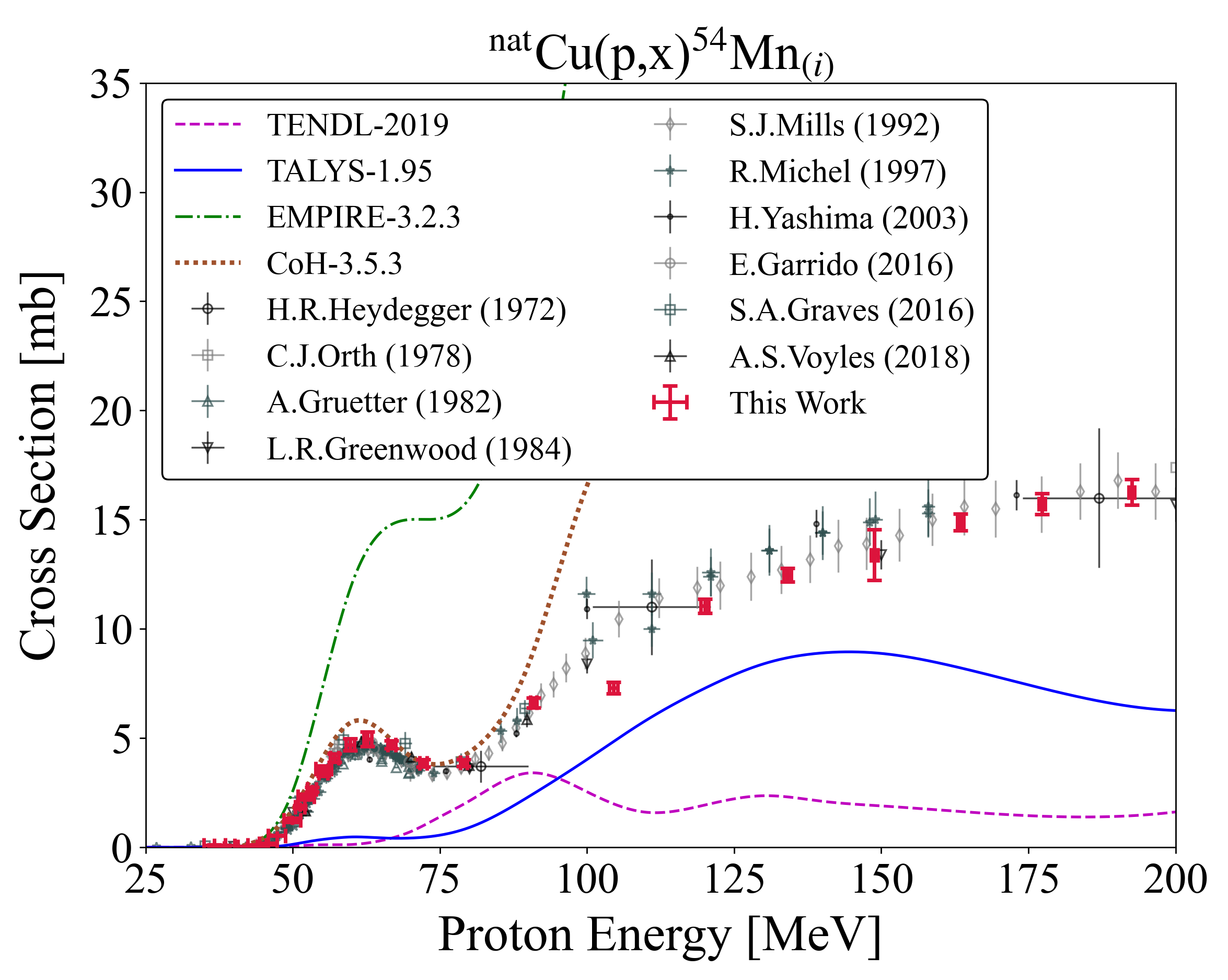
Figure 37: Experimental and theoretical cross sections for ⁵²Mn production.

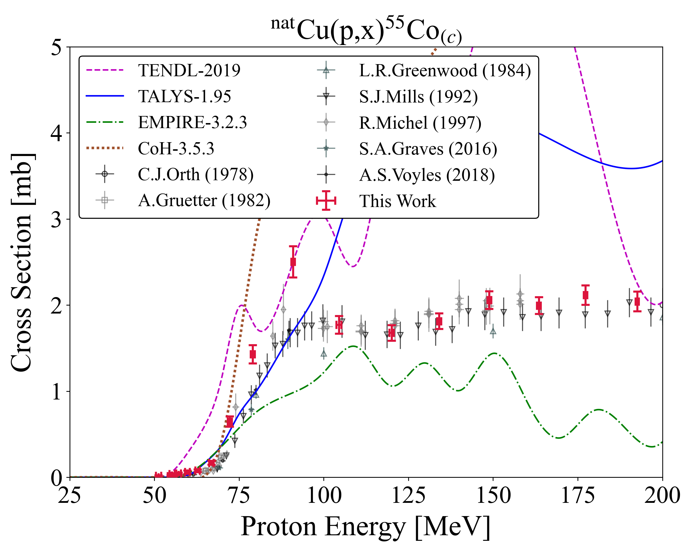
Figure 38: Experimental and theoretical cross sections for ⁵⁴Mn production.

Figure 39: Experimental and theoretical cross sections for ⁵⁵Co production.

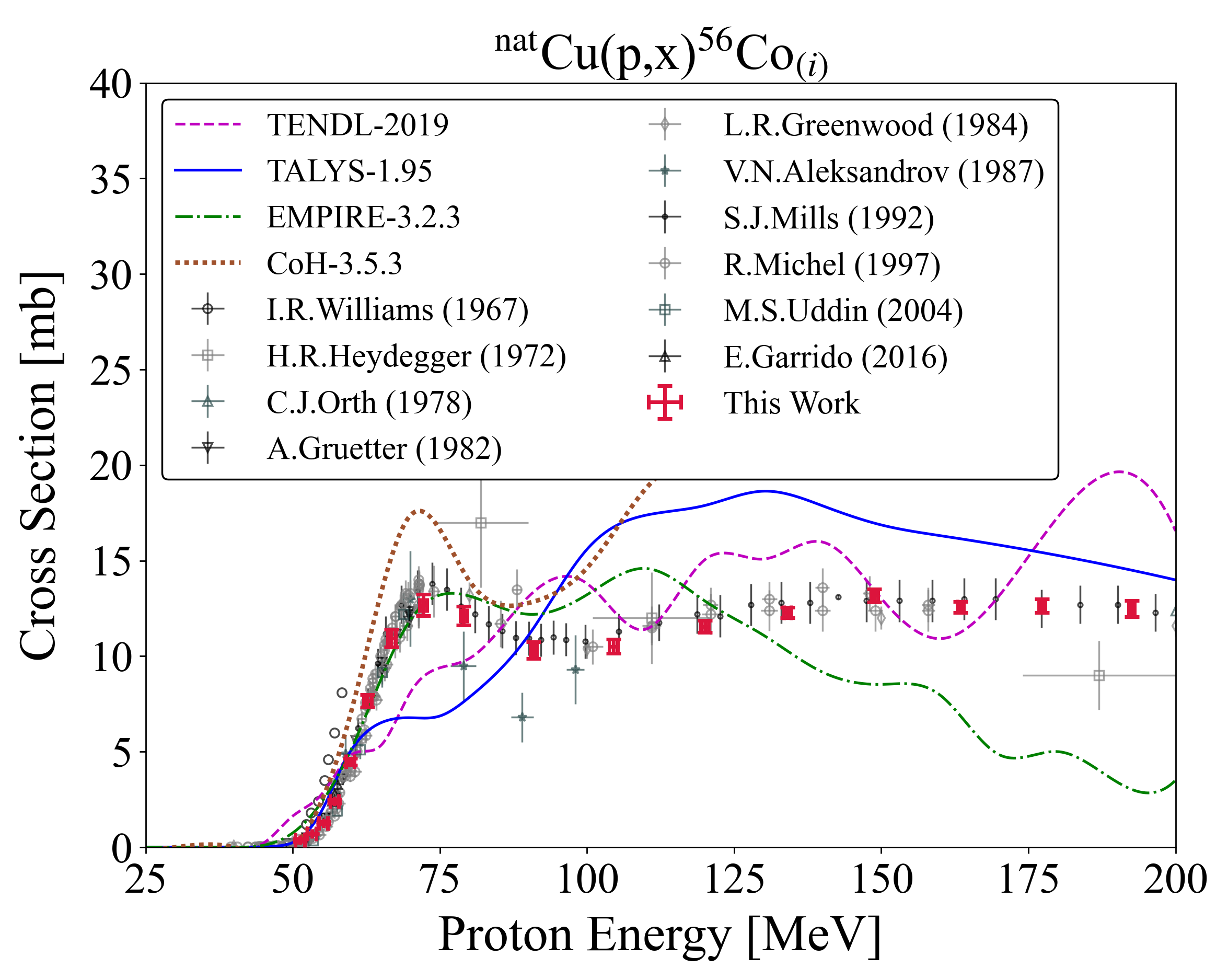
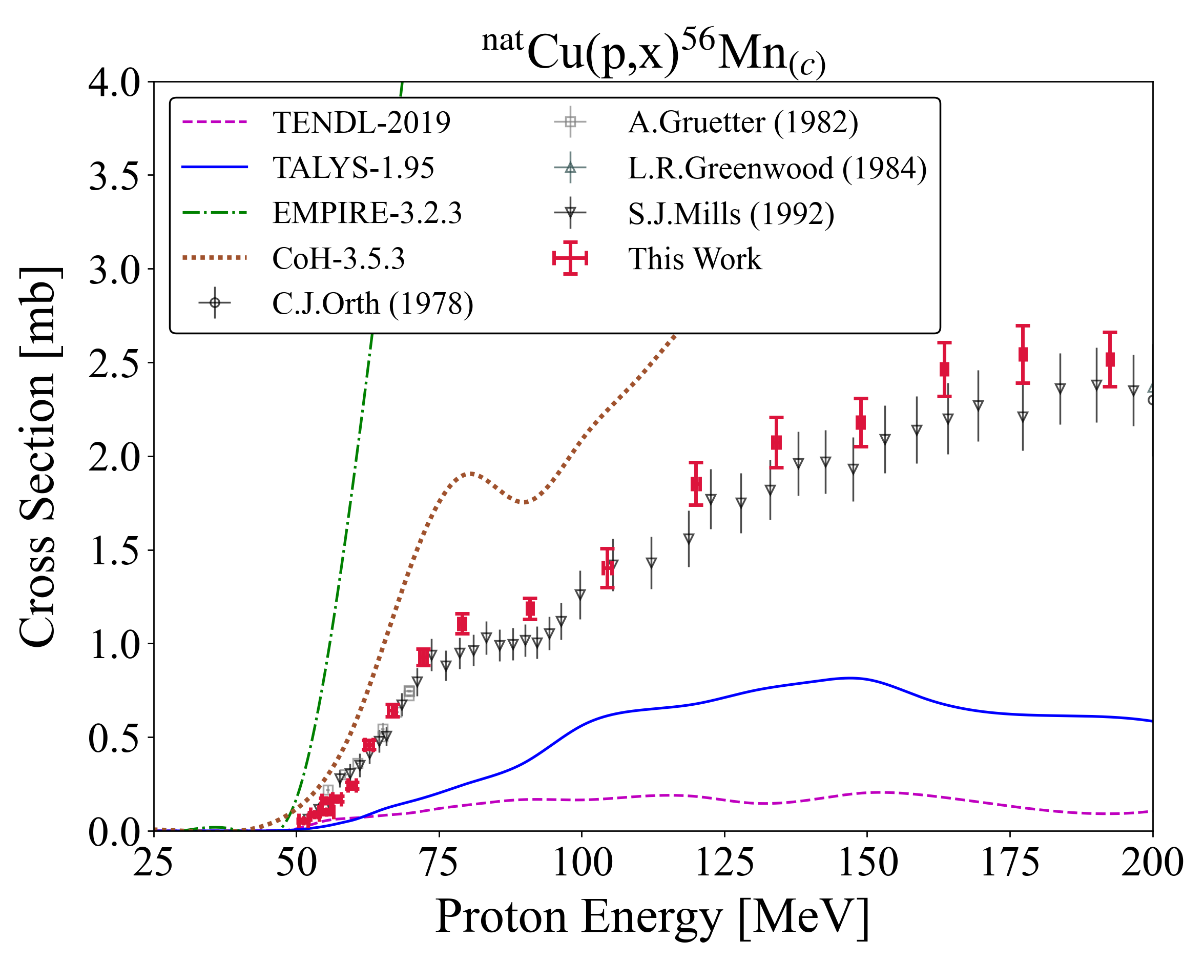
Figure 40: Experimental and theoretical cross sections for ⁵⁶Co production.

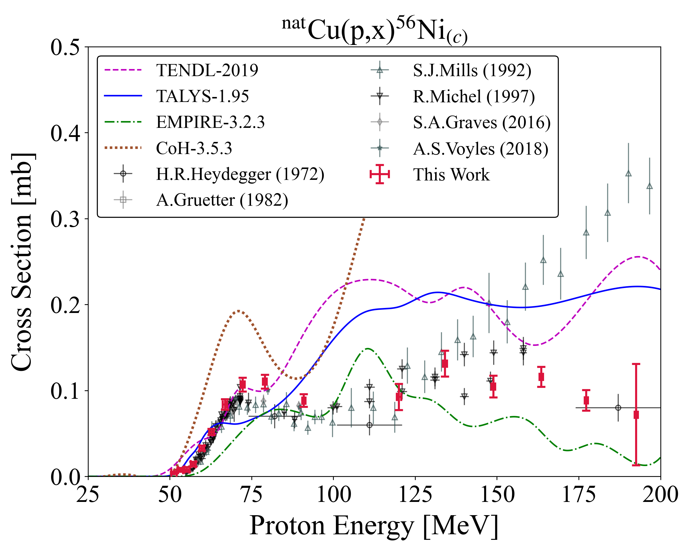
Figure 41: Experimental and theoretical cross sections for ⁵⁶Mn production.

Figure 42: Experimental and theoretical cross sections for ⁵⁶Ni production.

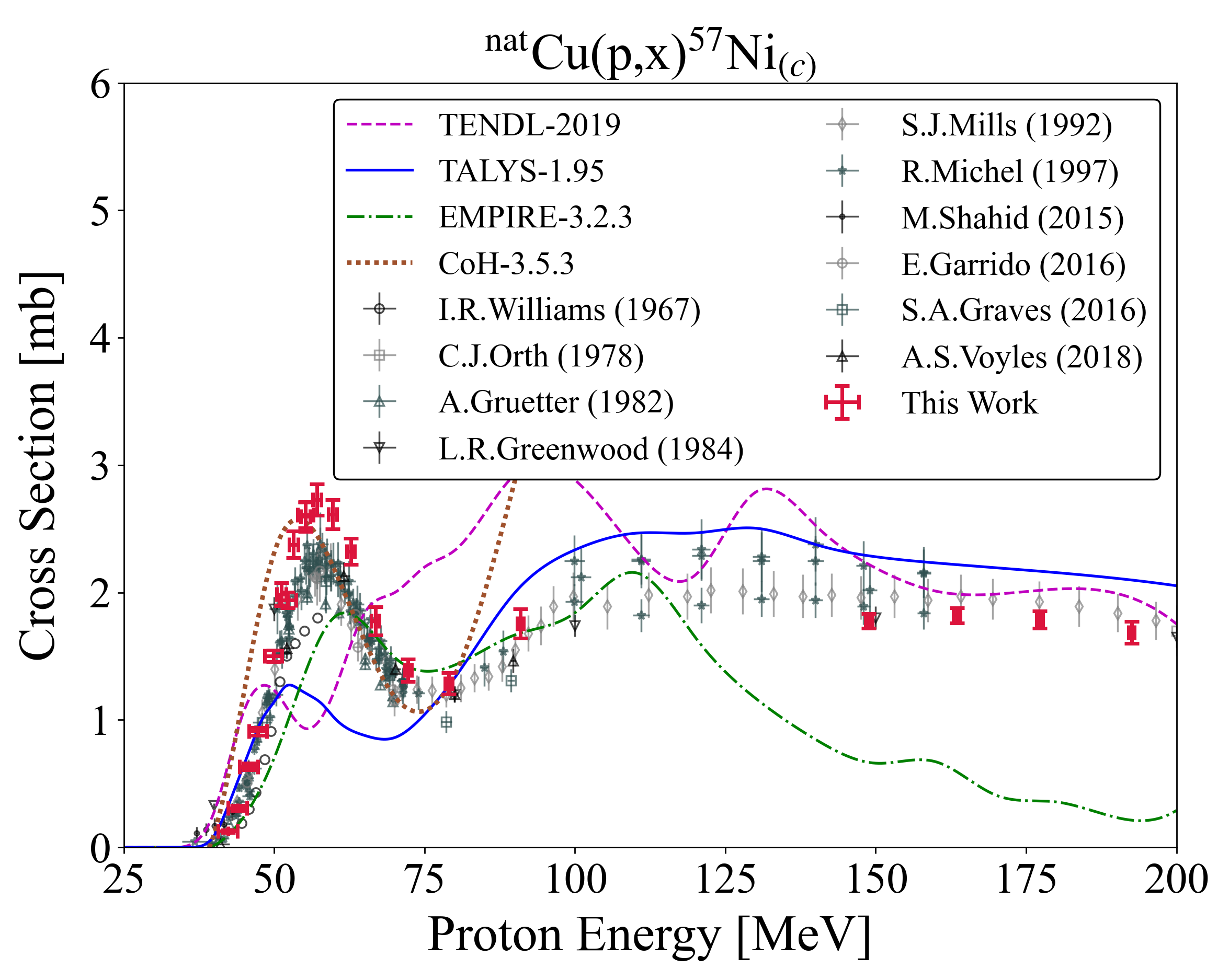
Figure 43: Experimental and theoretical cross sections for ⁵⁷Co production.

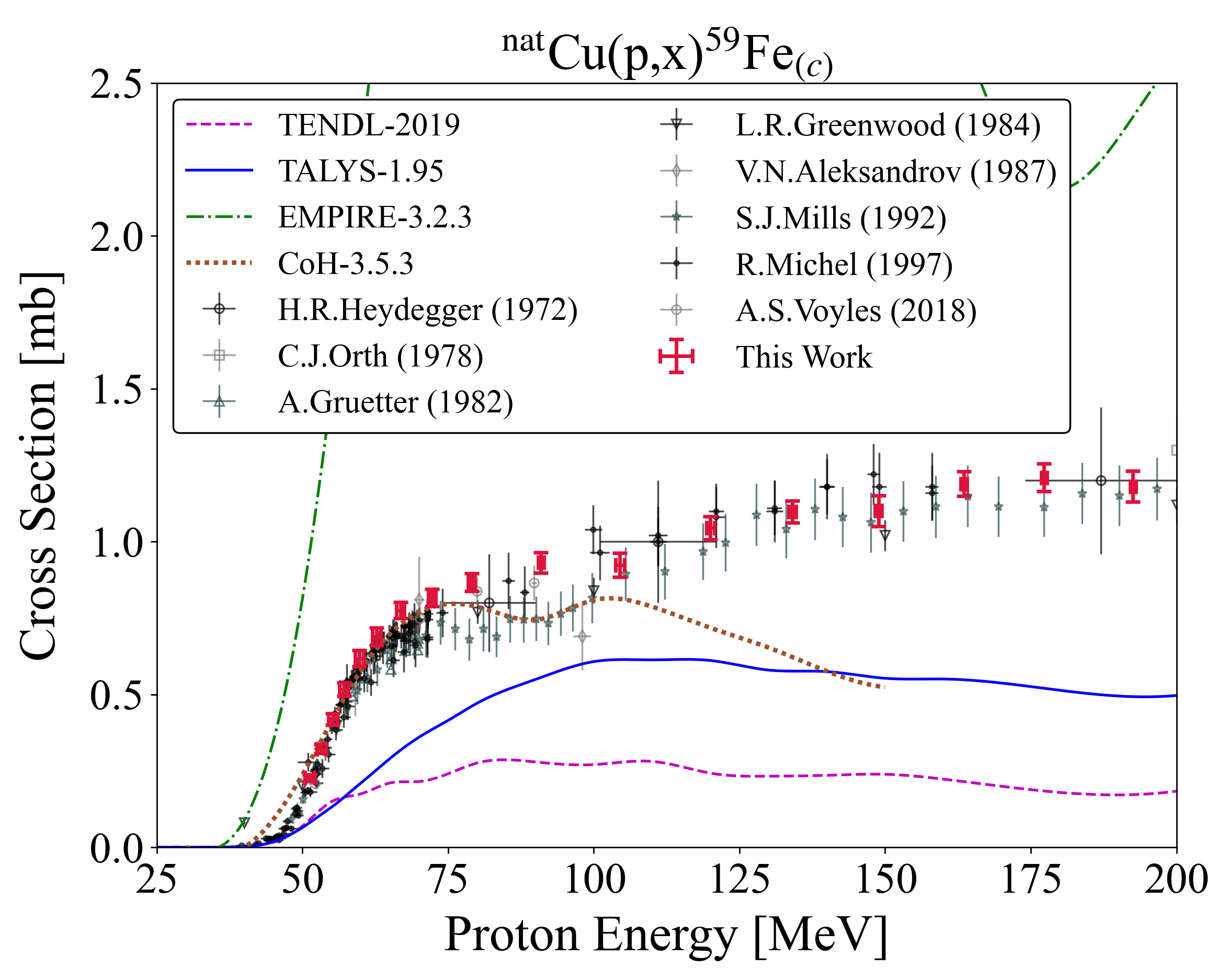
Figure 44: Experimental and theoretical cross sections for ⁵⁷Ni production.

Figure 45: Experimental and theoretical cross sections for ⁵⁹Fe production.

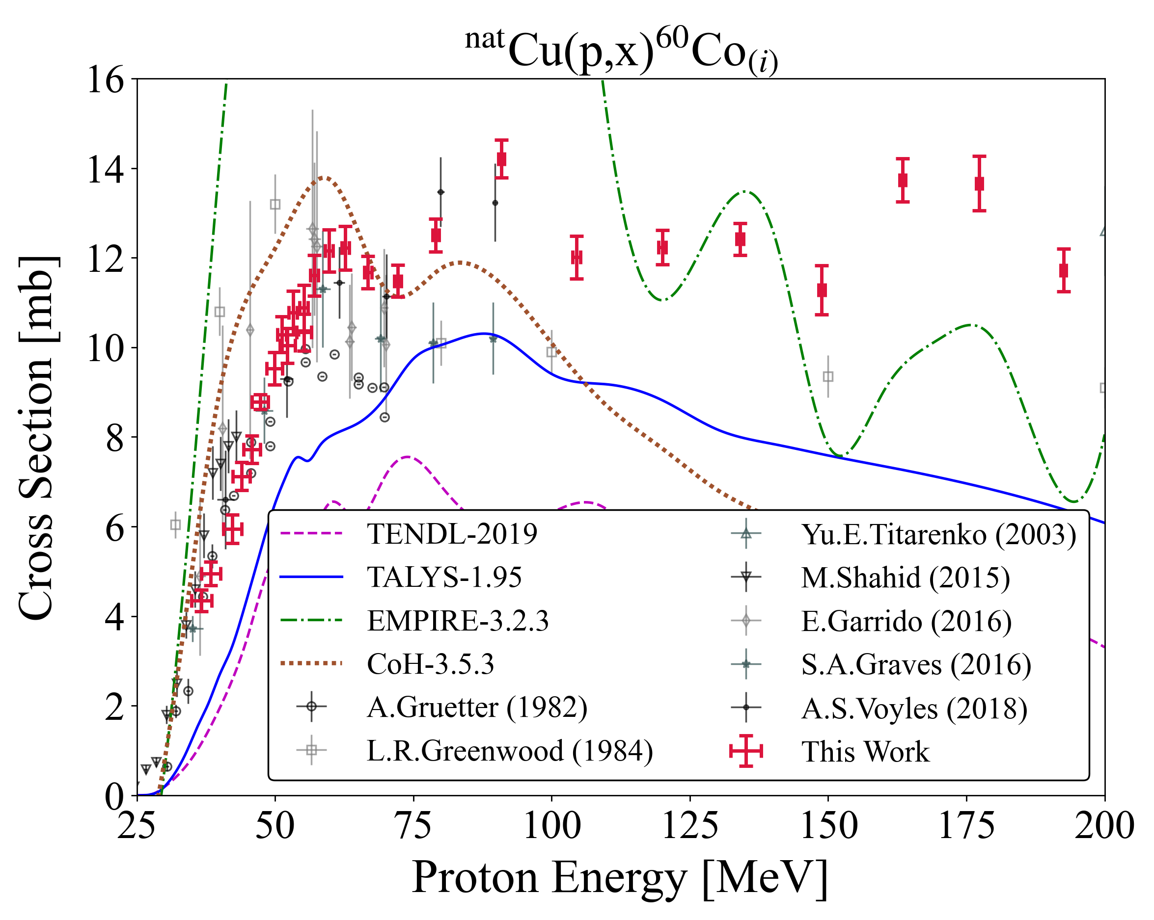
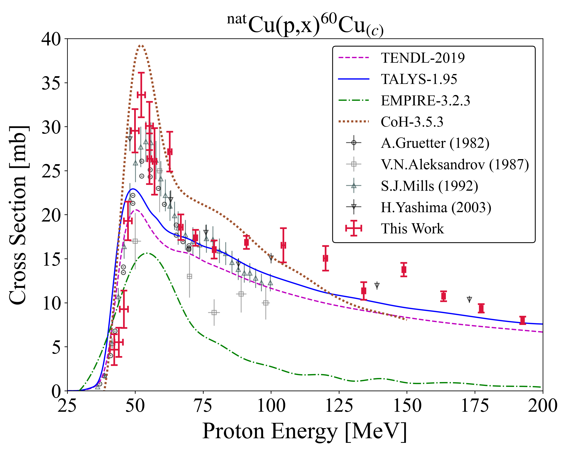
Figure 46: Experimental and theoretical cross sections for ⁶⁰Co production.

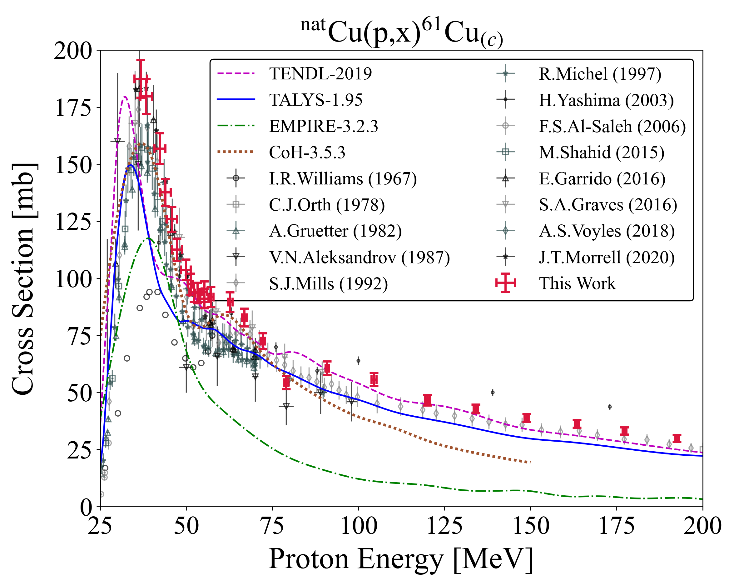
Figure 47: Experimental and theoretical cross sections for ⁶⁰Cu production.

Figure 48: Experimental and theoretical cross sections for ⁶¹Cu production.

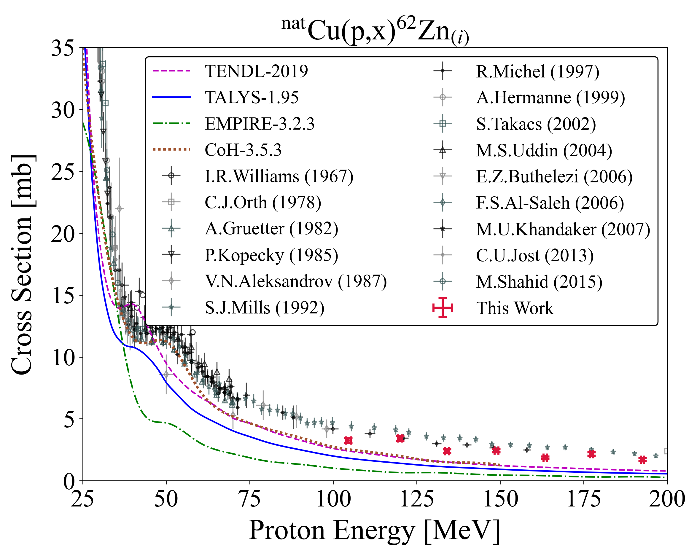
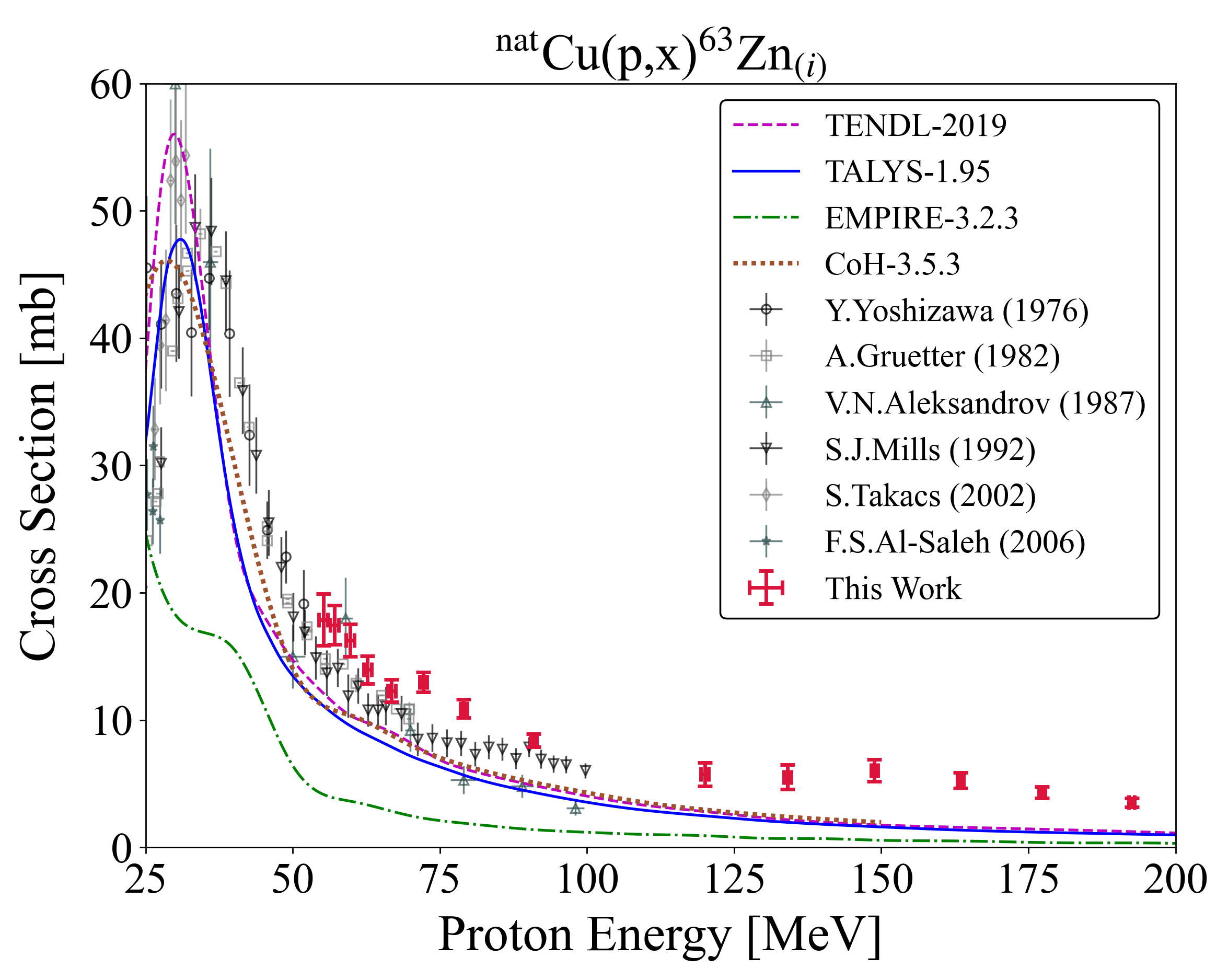
Figure 49: Experimental and theoretical cross sections for ⁶²Zn production.

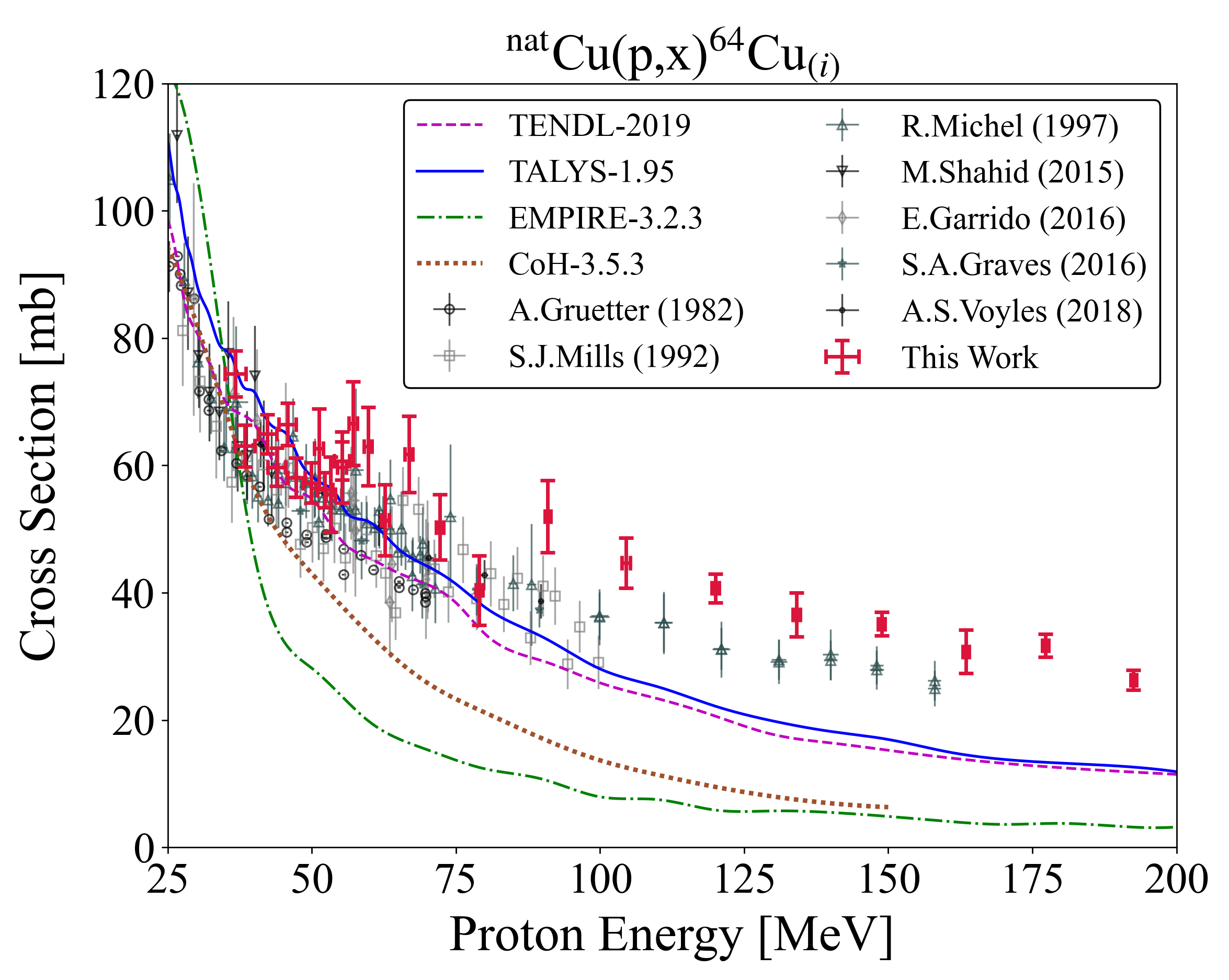
Figure 50: Experimental and theoretical cross sections for ⁶³Zn production.

Figure 51: Experimental and theoretical cross sections for ⁶⁴Cu production.

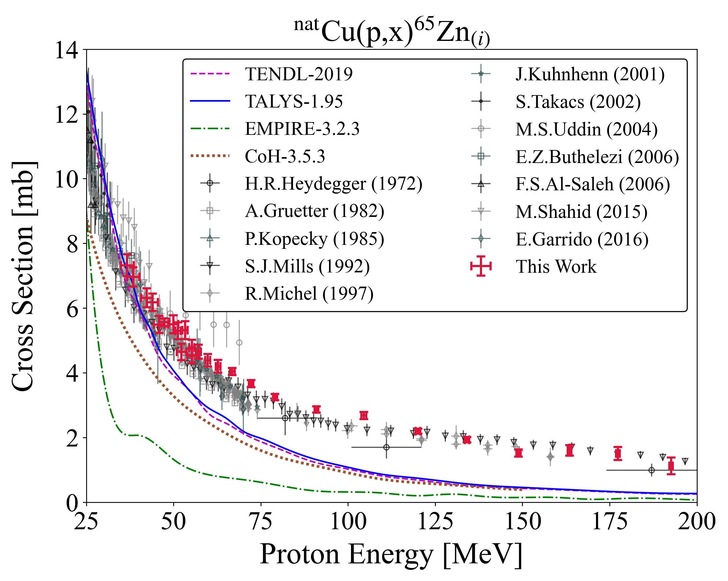
Figure 52: Experimental and theoretical cross sections for ⁶⁵Zn production.

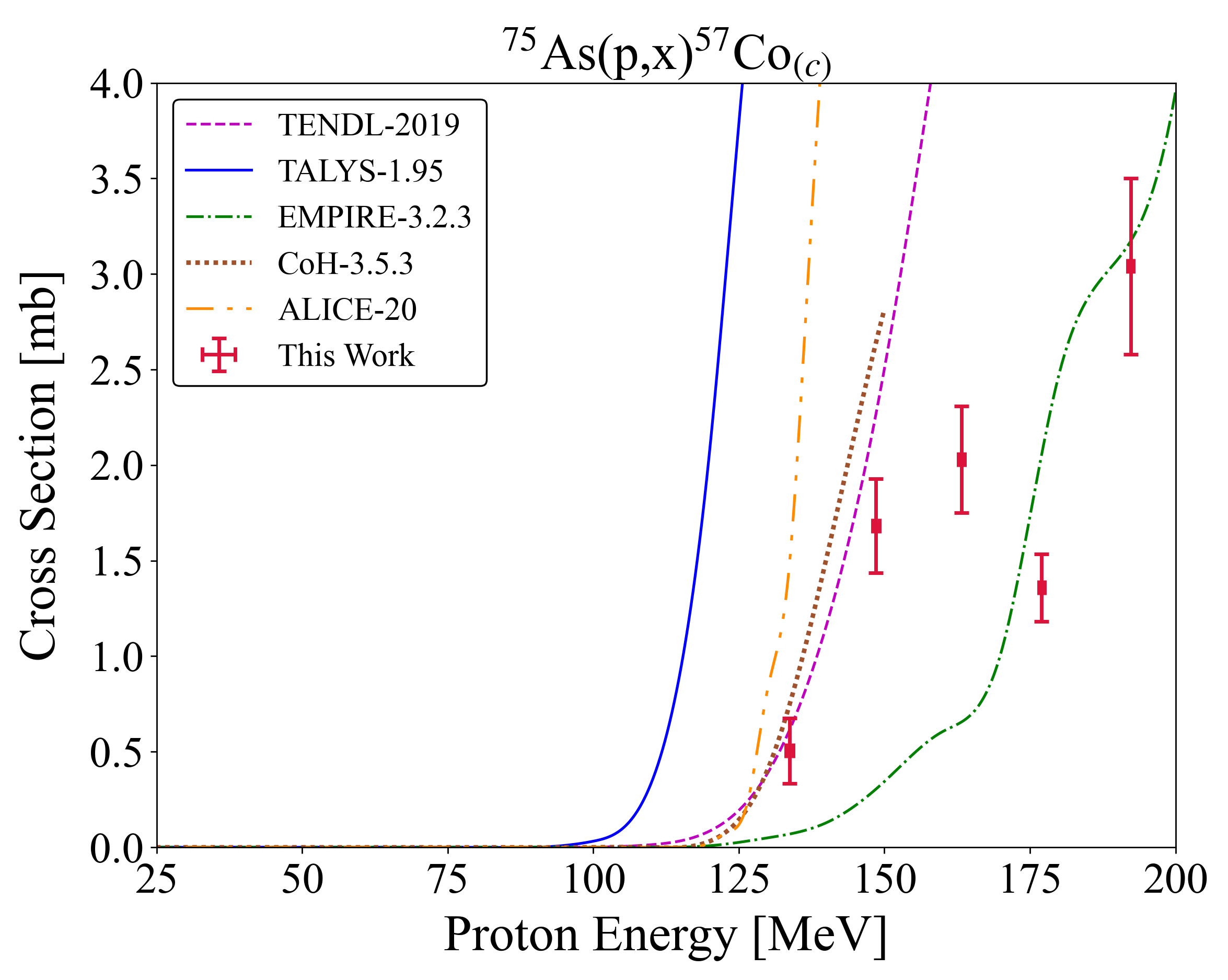
Figure 53: Experimental and theoretical cross sections for ⁵⁶Co production.

Figure 54: Experimental and theoretical cross sections for ⁵⁷Co production.

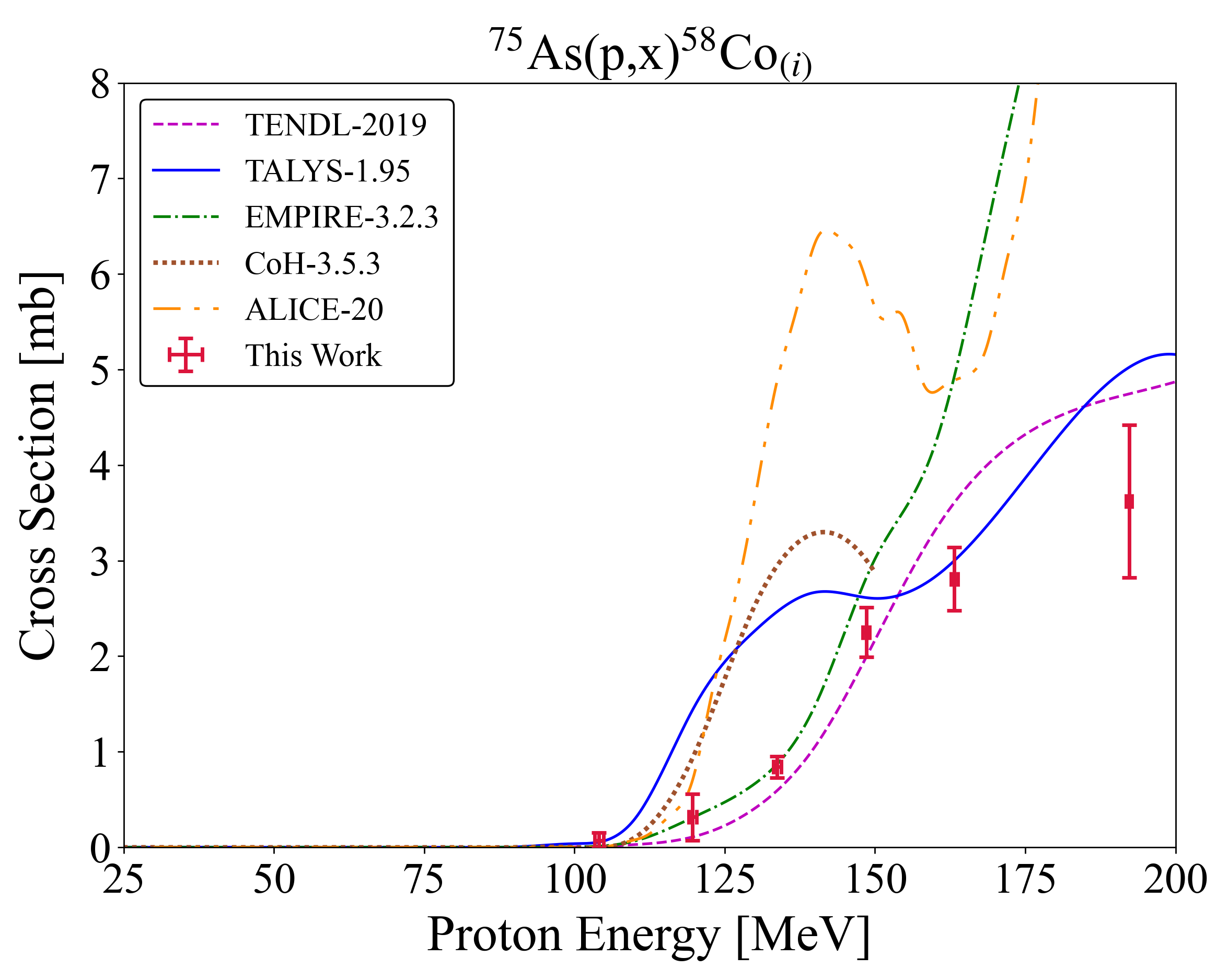
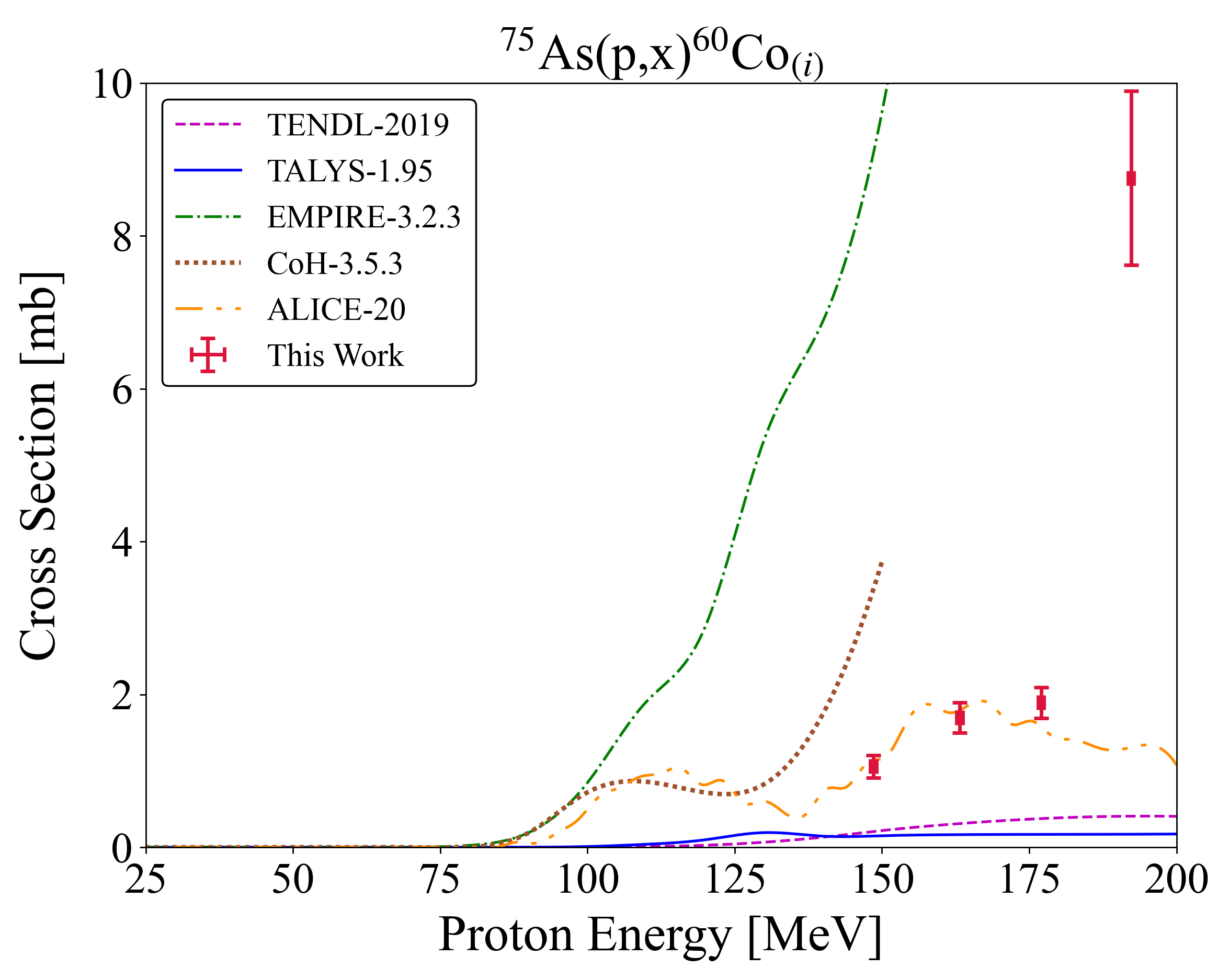
Figure 55: Experimental and theoretical cross sections for ⁵⁸Co production.

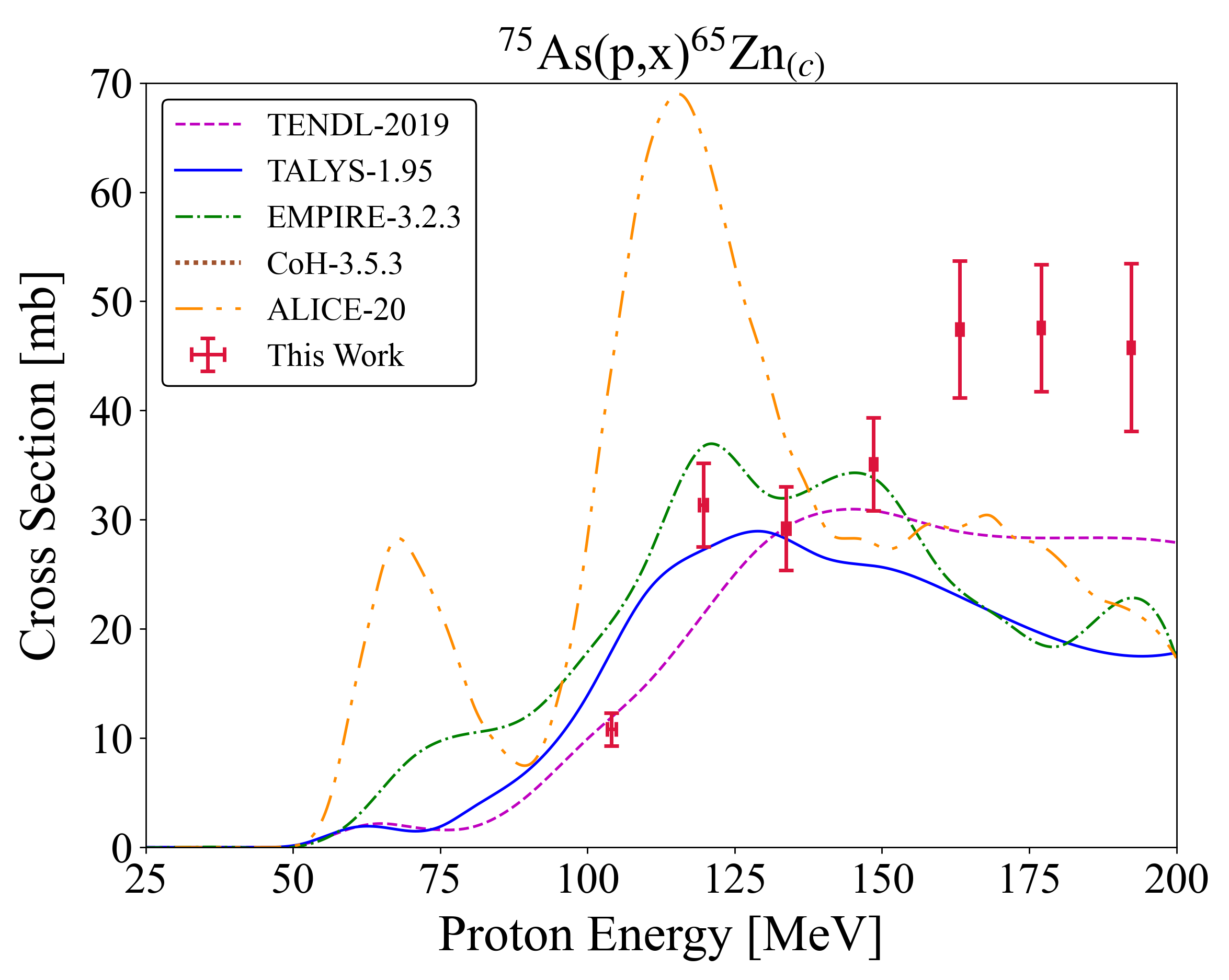
Figure 56: Experimental and theoretical cross sections for ⁶⁰Co production.

Figure 57: Experimental and theoretical cross sections for ⁶⁵Zn production.

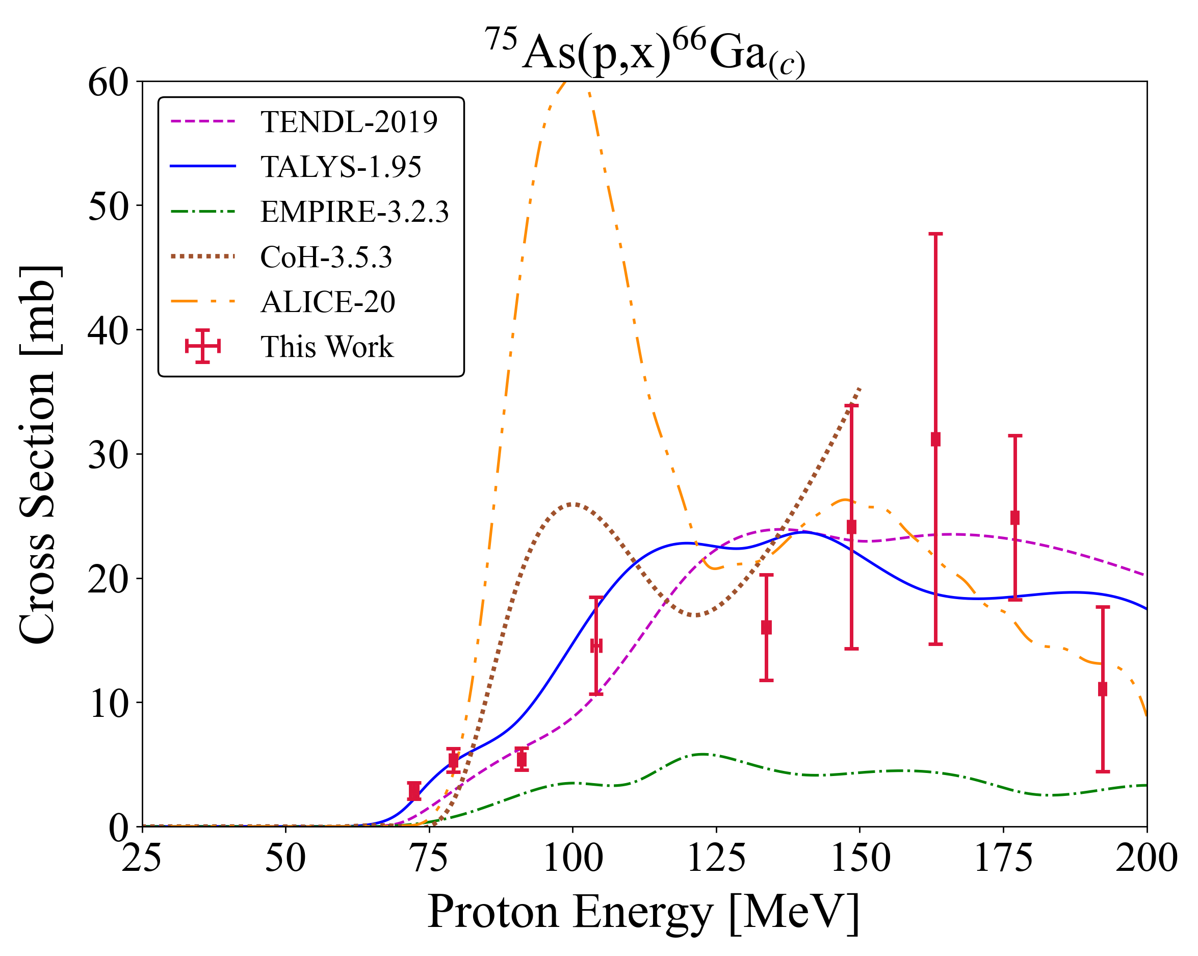
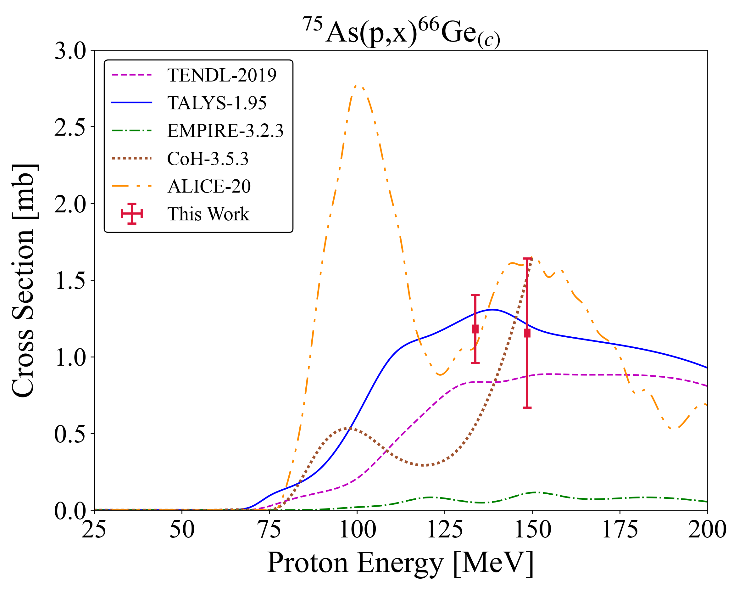
Figure 58: Experimental and theoretical cross sections for ⁶⁶Ga production.

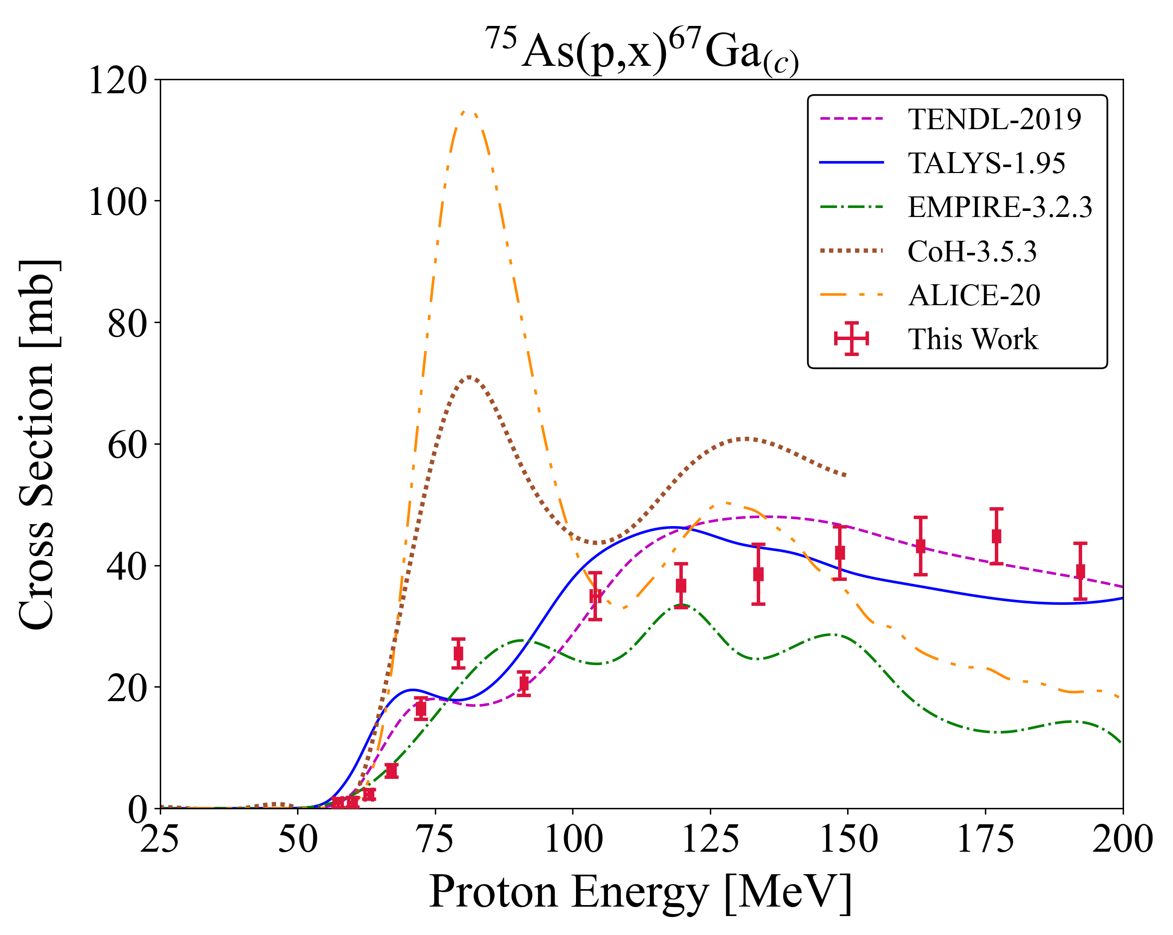
Figure 59: Experimental and theoretical cross sections for ⁶⁶Ge production.

Figure 60: Experimental and theoretical cross sections for ⁶⁷Ga production.

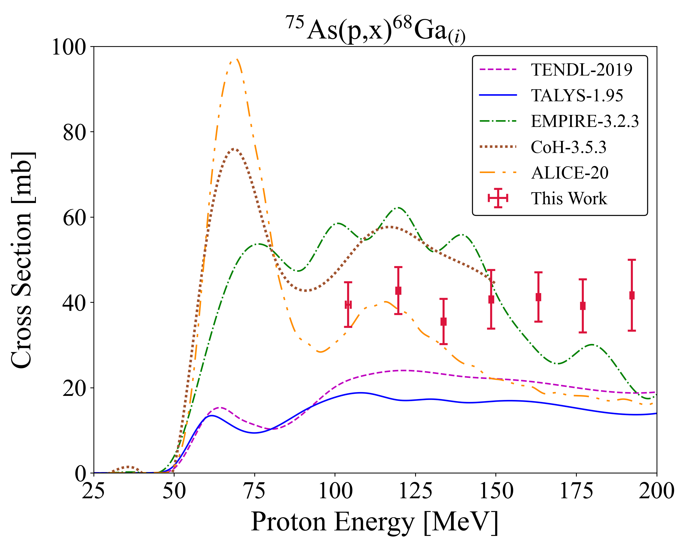
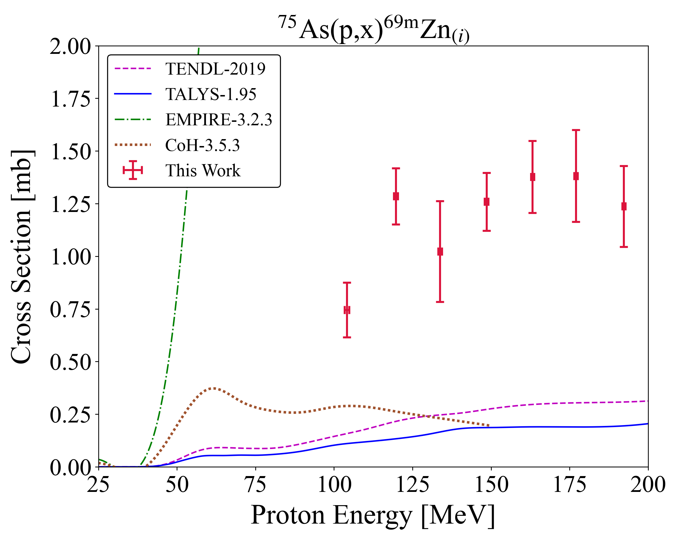
Figure 61: Experimental and theoretical cross sections for ⁶⁸Ga production.

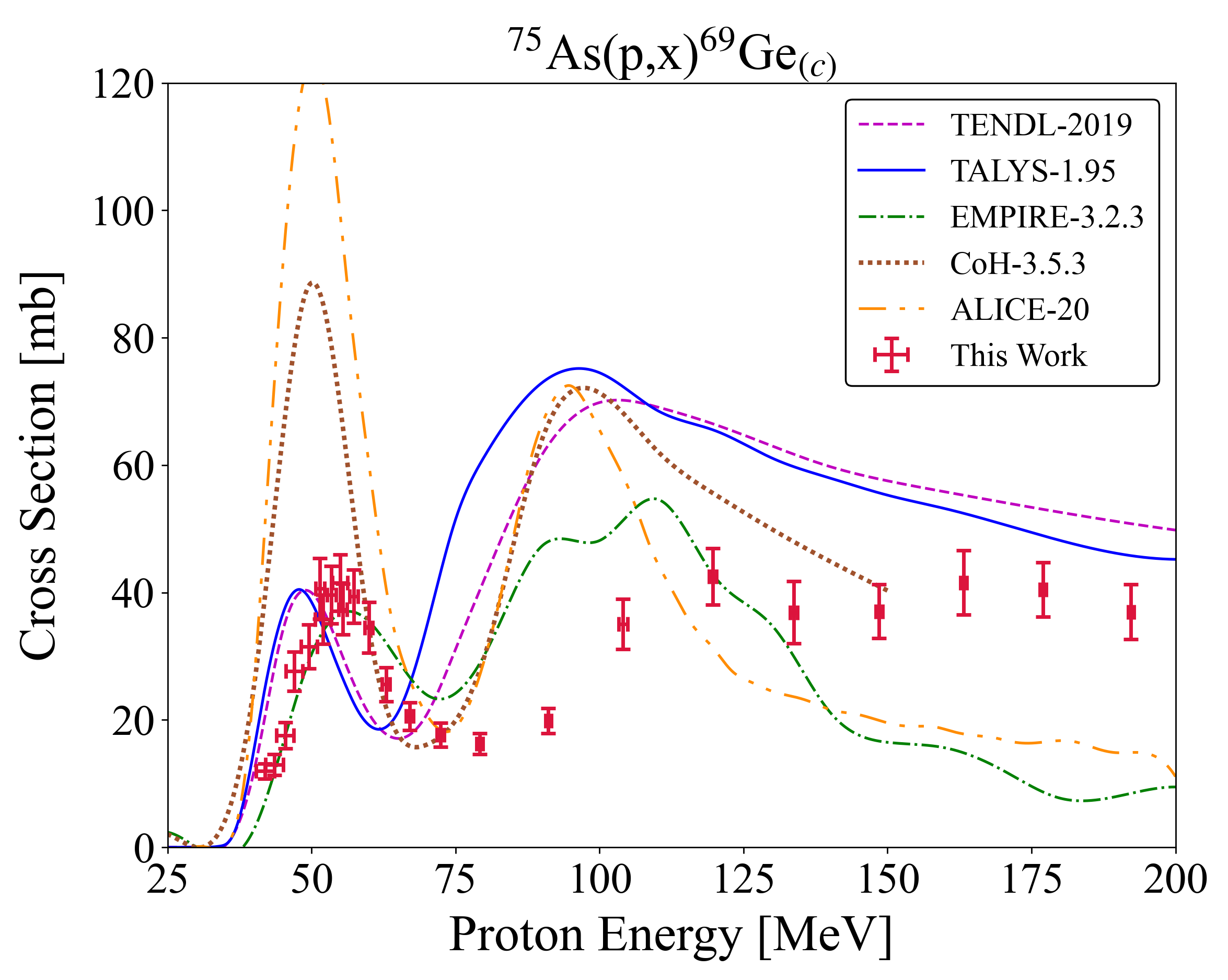
Figure 62: Experimental and theoretical cross sections for ${}^{\textnormal{69m}}$Zn production.

Figure 63: Experimental and theoretical cross sections for ⁶⁹Ge production.

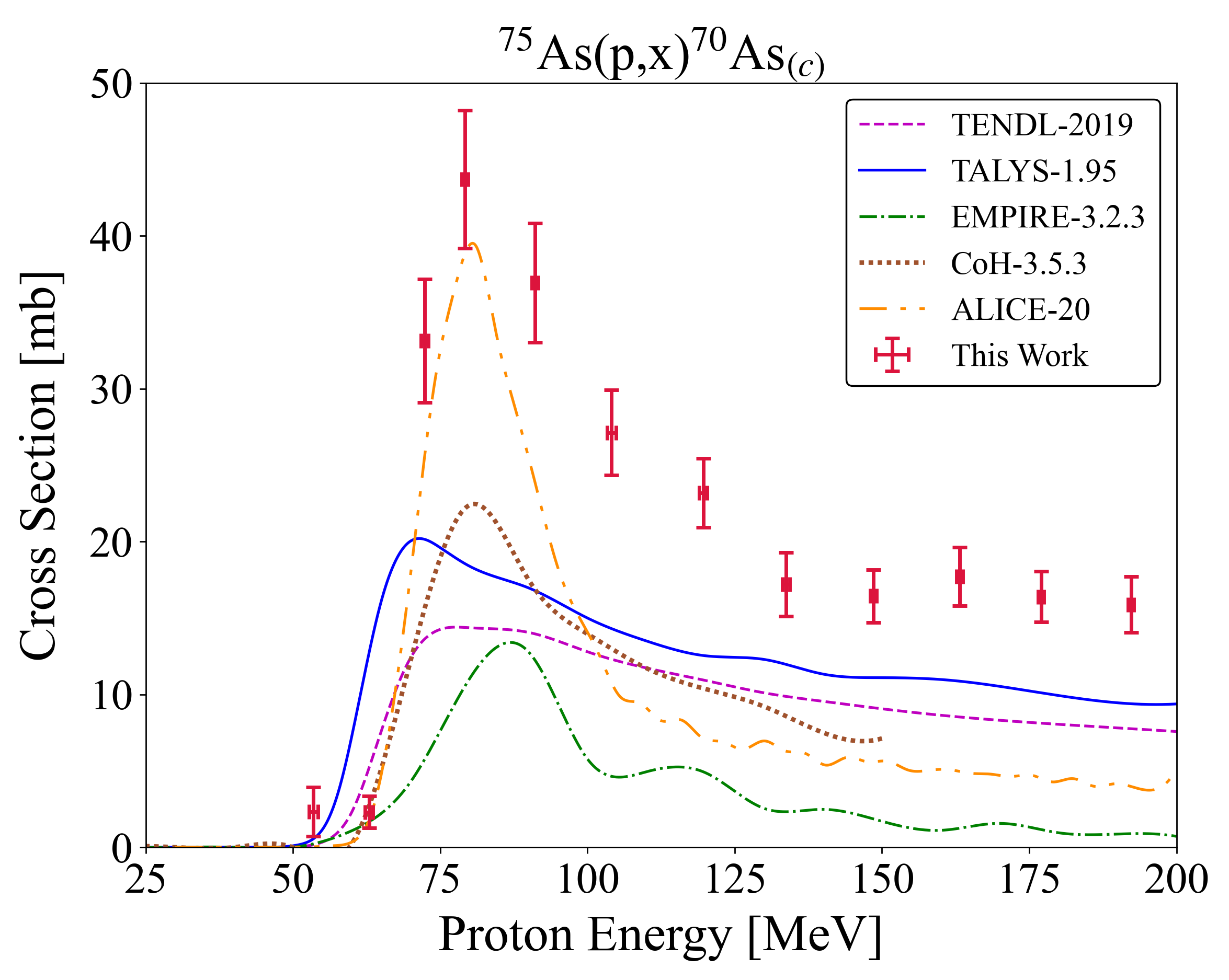
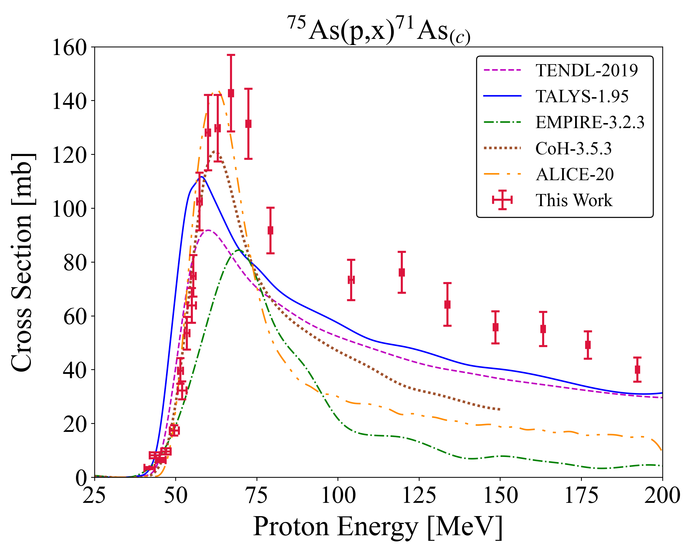
Figure 64: Experimental and theoretical cross sections for ⁷⁰As production.

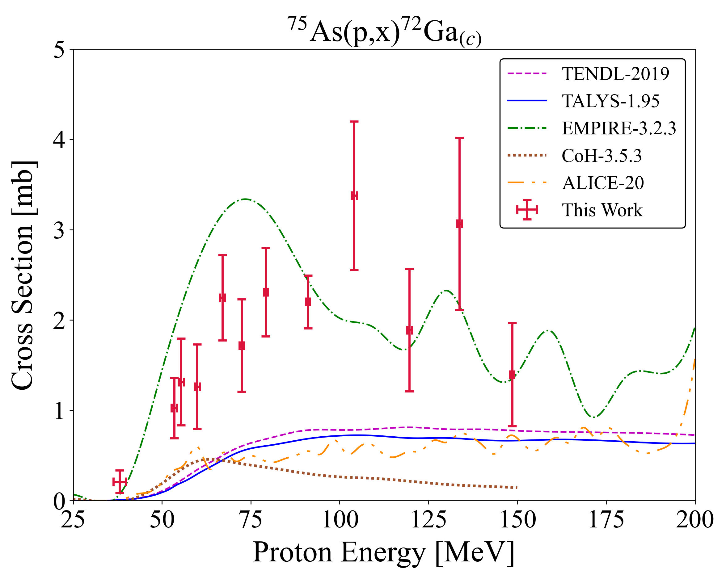
Figure 65: Experimental and theoretical cross sections for ⁷¹As production.

Figure 66: Experimental and theoretical cross sections for ⁷²Ga production.

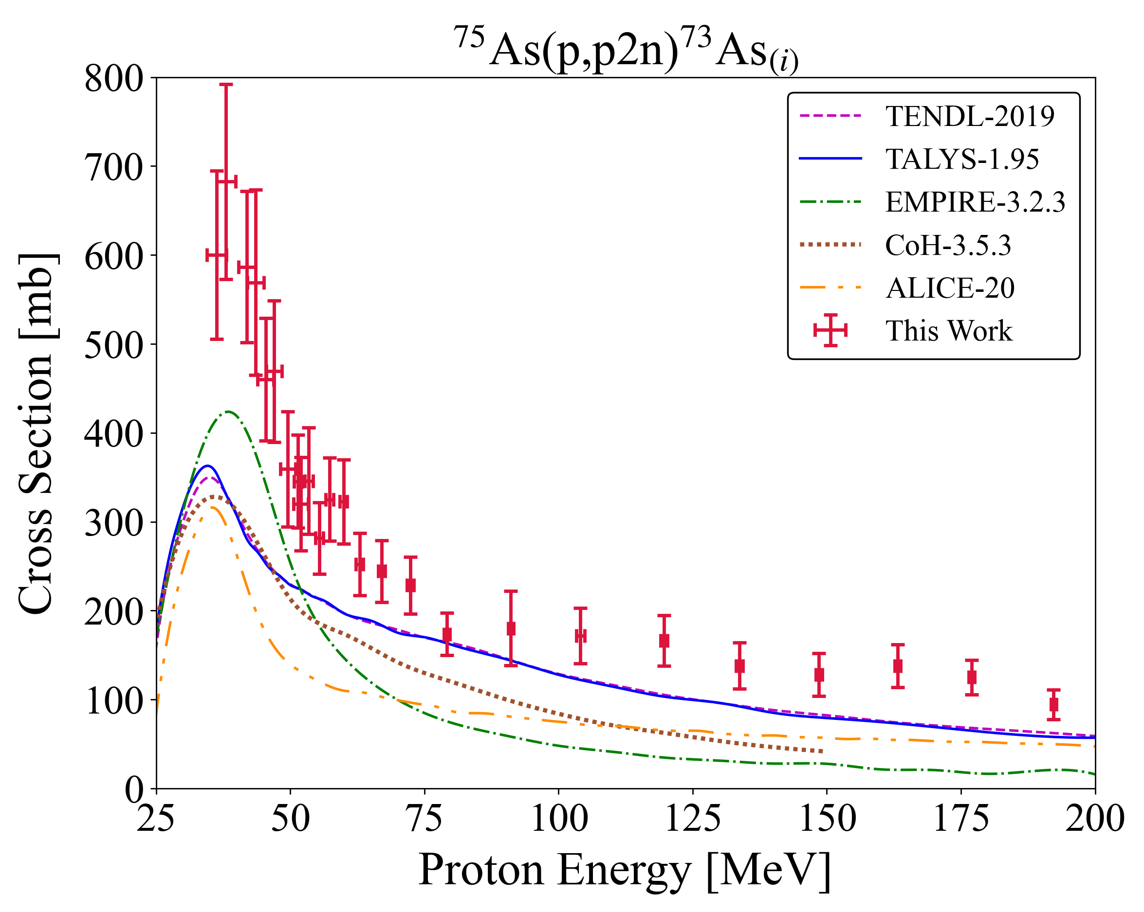
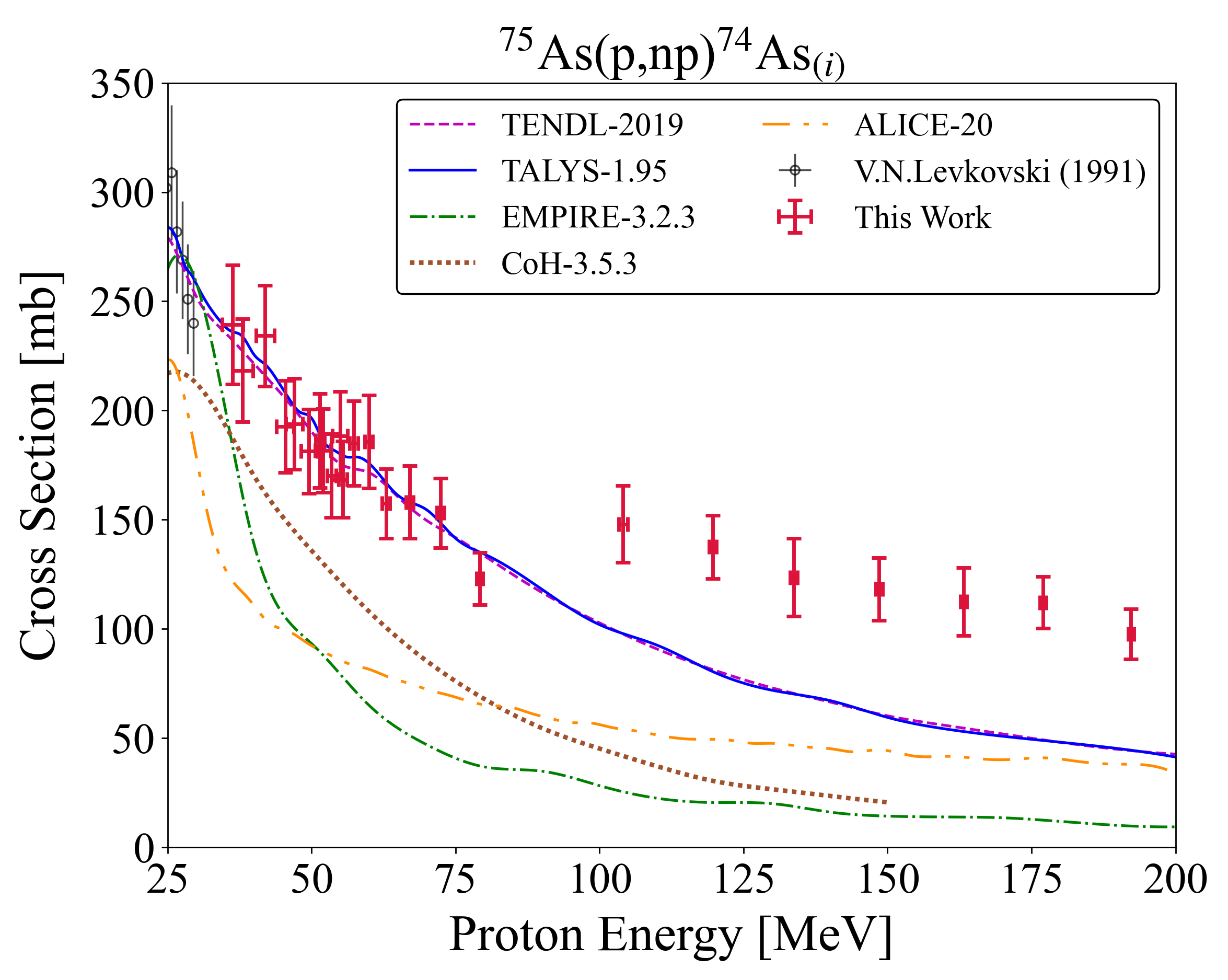
Figure 67: Experimental and theoretical cross sections for ⁷³As production.

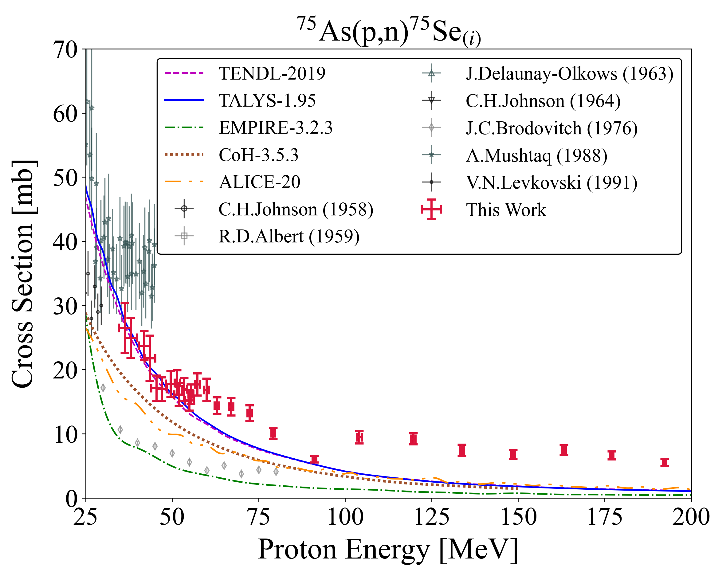
Figure 68: Experimental and theoretical cross sections for ⁷⁴As production.

Figure 69: Experimental and theoretical cross sections for ⁷⁵Se production.

Appendix D TALYS Parameter Adjustments From Fitting Procedure

The derived parameter adjustments from the fitting procedure applied to the ⁷⁵As(p,x) data are listed in Table 9.

Table 9: ⁷⁵As(p,x) best fit parameter adjustments derived from Fox et al. [21] procedure. The equidistant keyword adjusts the width of excitation energy binning and will be a default in updated TALYS versions. The strength keyword selects the gamma-ray strength model and has only a small impact in this charged-particle investigation. strength 8 performed comparably or slightly better than the other available models in TALYS.

Parameter	Value
ldmodel	6
	4 76-72Se, 68As
	5 69Ga
strength	8
equidistant	y
M2constant	0.80
M2limit	3.9
M2shift	0.55
Kph	15.16
d1adjust p	1.55
d1adjust n	1.75
w1adjust p	1.21
alphaomp	6
deuteronomp	4
Cstrip	a 0.85
	d 2.4
	h 0.55
	t 0.55
Cknock	a 0.85
	d 2.4
	h 0.55
	t 0.55
ctable	34 73 0.24
	33 74 0.3
	33 73 0.75
	33 71 -0.4
	32 69 0.285
	31 67 -0.45
ptable	34 73 -0.65
	34 72 0.14
	33 73 -1.85
	32 69 -0.25
	31 67 5.5

References

- Abriola and Sonzogni [2010] D. Abriola and A. A. Sonzogni, Nuclear Data Sheets for A = 72, Nuclear Data Sheets 111, 1 (2010).
- Jennewein et al. [2005] M. Jennewein, S. M. Qaim, P. V. Kulkarni, R. P. Mason, A. Hermanne, and F. Rösch, A no-carrier-added 72Se/72As radionuclide generator based on solid phase extraction, Radiochimica Acta 93, 579 (2005).
- Tárkányi et al. [2019] F. T. Tárkányi, A. V. Ignatyuk, A. Hermanne, R. Capote, B. V. Carlson, J. W. Engle, M. A. Kellet, T. Kibedi, G. N. Kim, F. G. Kondev, M. Hussain, O. Lebeda, A. Luca, Y. Nagai, H. Naik, A. L. Nichols, F. M. Nortier, S. V. Suryanarayana, S. Takacs, and M. Verpelli, Recommended nuclear data for medical radioisotope production: diagnostic positron emitters, Journal of Radioanalytical and Nuclear Chemistry 319, 533 (2019).
- Katakura and Wu [2008] J. Katakura and Z. D. Wu, Nuclear Data Sheets for A = 124, Nuclear Data Sheets 109, 1655 (2008).
- Cascini et al. [2014] G. L. Cascini, A. N. Asabella, A. Notaristefano, A. Restuccia, C. Ferrari, D. Rubini, C. Altini, and G. Rubini, 124Iodine: A Longer-Life Positron Emitter Isotope - New Opportunities in Molecular Imaging, BioMed Research International 2014, 1 (2014).
- Singh and Nica [2012] B. Singh and N. Nica, Nuclear Data Sheets for A = 77, Nuclear Data Sheets 113, 1115 (2012).
- DeGraffenreid et al. [2019] A. J. DeGraffenreid, D. G. Medvedev, T. E. Phelps, M. D. Gott, S. V. Smith, S. S. Jurisson, and C. S. Cutler, Cross-section measurements and production of Se with medium to high energy protons using arsenic containing targets, Radiochimica Acta 107, 279 (2019).
- Jennewein et al. [2008] M. Jennewein, M. A. Lewis, D. Zhao, E. Tsyganov, N. Slavine, J. He, L. Watkins, V. D. Kodibagkar, S. O. Kelly, P. Kulkarni, P. P. Antich, A. Hermanne, F. Ro, R. P. Mason, and P. E. Thorpe, Vascular Imaging of Solid Tumors in Rats with a Radioactive Arsenic-Labeled Antibody that Binds Exposed Phosphatidylserine, Clinical Cancer Research 14, 1377 (2008).
- Sanders and Cutler [2021] V. A. Sanders and C. S. Cutler, Radioarsenic: A promising theragnostic candidate for nuclear medicine, Nuclear Medicine and Biology 92, 184 (2021).
- Ellison et al. [2017] P. A. Ellison, T. E. Barnhart, F. Chen, H. Hong, Y. Zhang, C. P. Theuer, W. Cai, R. J. Nickles, and O. T. DeJesus, High Yield Production and Radiochemical Isolation of Isotopically Pure Arsenic-72 and Novel Radioarsenic Labeling Strategies for the Development of Theranostic Radiopharmaceuticals, Bioconjugate Chemistry 27, 179 (2017).
- Ballard et al. [2012a] B. Ballard, F. M. Nortier, E. R. Birnbaum, K. D. John, D. R. Phillips, and M. Fassbender, Radioarsenic from a Portable 72Se/72As Generator: A Current Perspective, Current Radiopharmaceuticals 5, 264 (2012a).
- Ballard et al. [2012b] B. Ballard, D. Wycoff, E. R. Birnbaum, K. D. John, J. W. Lenz, S. S. Jurisson, C. S. Cutler, F. M. Nortier, W. A. Taylor, and M. E. Fassbender, Selenium-72 formation via natBr(p,x) induced by 100MeV Protons: Steps towards a novel 72Se/ 72As generator system, Applied Radiation and Isotopes 70, 595 (2012b).
- Fassbender et al. [2001] M. Fassbender, D. De Villiers, M. Nortier, and N. Van der Walt, The natBr(p,x)73,75Se nuclear processes: a convenient route for the production of radioselenium tracers relevant to amino acid labelling, Applied Radiation and Isotopes 54, 905 (2001).
- Takács et al. [2016] S. Takács, M. P. Takács, F. Ditrói, M. Aikawa, H. Haba, and Y. Komori, Activation cross sections of longer-lived radionuclides produced in germanium by alpha particle irradiation, Nuclear Instruments and Methods in Physics Research B 383, 213 (2016).
- McCutchan [2012] E. A. McCutchan, Nuclear Data Sheets for A = 68, Nuclear Data Sheets 113, 1735 (2012).
- Martiniova et al. [2016] L. Martiniova, L. D. Palatis, E. Etchebehere, and G. Ravizzini, Gallium-68 in Medical Imaging, Current Radiopharmaceuticals 9, 187 (2016).
- Roesch and Filosofov [2010] F. Roesch and D. V. Filosofov, Production of Long Lived Parent Radionuclides for Generators : 68Ge, 82Sr, 90Sr and 188W, IAEA Radioisotopes and Radiopharmaceuticals Series 2 (2010).
- Burke and Archibald [2020] B. P. Burke and S. J. Archibald, Handbook of Radiopharmaceuticals: Methodology and Applications, 2nd ed., edited by P. Scott and M. Kilbourn (2020) pp. 291–323.
- Beard et al. [2010] C. Beard, D. L. Clark, G. D. Jarvinen, A. Migliori, W. Runde, M. Coonley, K. Parker, E. Lorusso, and L. Archuleta, Accelerator Radioisotopes Save Lives: Part II, Actinide Research Quarterly (LALP-10-011) , 1 (2010).
- Kratochwil et al. [2018] C. Kratochwil, F. Bruchertseifer, H. Rathke, M. Hohenfellner, F. L. Giesel, U. Haberkorn, and A. Morgenstern, Targeted -Therapy of Metastatic Castration-Resistant Prostate Cancer with 225Ac-PSMA-617: Swimmer-Plot Analysis Suggests Efficacy Regarding Duration of Tumor Control, Journal of Nuclear Medicine 59, 795 (2018).
- Fox et al. [2021] M. B. Fox, A. S. Voyles, J. T. Morrell, L. A. Bernstein, A. M. Lewis, A. J. Koning, J. C. Batchelder, E. R. Birnbaum, C. S. Cutler, D. G. Medvedev, F. M. Nortier, E. M. O’Brien, and C. Vermeulen, Investigating high-energy proton-induced reactions on spherical nuclei: Implications for the preequilibrium exciton model, Physical Review C 103, 034601 (2021).
- Hogle et al. [2021] S. Hogle, E. O’Brien, A. S. Voyles, K. Kolos, and V. Sobes, Predictive Codes for Isotope Production, in Workshop for Applied Nuclear Data Activities (WANDA 2021) (Washington, D.C., 2021).
- Voyles et al. [2018] A. S. Voyles, L. A. Bernstein, E. R. Birnbaum, J. W. Engle, S. A. Graves, T. Kawano, A. M. Lewis, and F. M. Nortier, Excitation functions for (p,x) reactions of niobium in the energy range of E MeV, Nuclear Instruments and Methods in Physics Research B 429, 53 (2018).
- Morrell et al. [2020] J. T. Morrell, A. S. Voyles, M. S. Basunia, J. C. Batchelder, E. F. Matthews, and L. A. Bernstein, Measurement of 139La(p,x) cross sections from 35-60 MeV by stacked-target activation, The European Physical Journal A 56, 13 (2020).
- Graves et al. [2016] S. A. Graves, P. A. Ellison, T. E. Barnhart, H. F. Valdovinos, R. Eva, F. M. Nortier, R. J. Nickles, and J. W. Engle, Nuclear excitation functions of proton-induced reactions (E MeV) from Fe, Cu, Al, Nuclear Instruments and Methods in Physics Research B 386, 44 (2016).
- Engle et al. [2013] J. W. Engle, S. G. Mashnik, J. W. Weidner, L. E. Wolfsberg, M. Fassbender, K. Jackman, A. Couture, L. J. Bitteker, J. L. Ullmann, M. S. Gulley, C. Pillai, K. D. John, E. R. Birnbaum, and F. M. Nortier, Cross sections from proton irradiation of thorium at 800 MeV, Physical Review C 88, 014604 (2013).
- Engle et al. [2016] J. W. Engle, S. G. Mashnik, L. A. Parker, K. R. Jackman, L. J. Bitteker, J. L. Ullmann, M. S. Gulley, C. Pillai, K. D. John, E. R. Birnbaum, and F. M. Nortier, Nuclear excitation functions from 40 to 200 MeV proton irradiation of terbium, Nuclear Instruments and Methods in Physics Research B 366, 206 (2016).
- Voyles et al. [2021a] A. S. Voyles, M. B. Fox, J. T. Morrell, M. P. Zach, E. K. Still, L. A. Bernstein, W. D. Frey, and B. J. Mehciz, Preparation and Characterization of Thin Arsenic Targets for Stacked-Target Experiments, arXiv (2021a), arXiv:2106.05524 .
- Gallagher and Cipolla [1974] W. J. Gallagher and S. J. Cipolla, A Model-Based Efficiency Calibration of a Si(Li) Detector in the Energy Region From 3 to 140 keV, Nuclear Instruments and Methods 122, 405 (1974).
- Morrell [2020] J. T. Morrell, Curie: Python Toolkit for Experimental Nuclear Data (2020).
- Morrell [2019] J. T. Morrell, NPAT: Nuclear physics analysis tools (2019).
- Hermanne et al. [2018] A. Hermanne, A. V. Ignatyuk, R. Capote, B. V. Carlson, J. W. Engle, M. A. Kellett, and T. Kib, Reference Cross Sections for Charged-particle Monitor Reactions, Nuclear Data Sheets 148, 338 (2018).
- Voyles et al. [2021b] A. S. Voyles, A. M. Lewis, J. T. Morrell, M. Shamsuzzoha Basunia, L. A. Bernstein, J. W. Engle, S. A. Graves, and E. F. Matthews, Proton-induced reactions on Fe, Cu, & Ti from threshold to 55 MeV, European Physics Journal A 57, 1 (2021b).
- Koning et al. [2019] A. J. Koning, S. Hilaire, and S. Goriely, TALYS-1.95 - A Nuclear Reaction Program (2019).
- Kawano [2019] T. Kawano, Unified Coupled-Channels and Hauser-Feshbach Model Calculation for Nuclear Data Evaluation (LA-UR 19-20315), Tech. Rep. (2019) arXiv:1901.05641 .
- Herman et al. [2007] M. Herman, R. Capote, B. V. Carlson, P. Oblozinsky, M. Sin, A. Trkov, H. Wienke, and V. Zerkin, EMPIRE: Nuclear Reaction Model Code System for Data Evaluation, Nuclear Data Sheets 108, 2655 (2007).
- Blann and Bisplinghoff [1982] M. Blann and J. Bisplinghoff, ALICE/LIVERMORE Precompound Compound Decay, Tech. Rep. (Lawrence Livermore National Laboratory, 1982).
- Koning and Rochman [2012] A. J. Koning and D. Rochman, Modern Nuclear Data Evaluation with the TALYS Code System, Nuclear Data Sheets 113, 2841 (2012).
- Mushtaq et al. [1988] A. Mushtaq, S. M. Qaim, and G. Stöcklin, Production of 73Se via (p, 3n) and (d, 4n) Reactions on Arsenic, International Journal of Radiation Applications and Instrumentation Part A 39, 1085 (1988).
- Qaim et al. [1988] S. M. Qaim, A. Mushtaq, and M. Uhl, Isomeric cross-section ratio for the formation of 73m,gSe in various nuclear processes, Physical Review C 38, 645 (1988).
- Brodovitch et al. [1976] J. C. Brodovitch, J. J. Hogan, and K. Burns, The Pre-equilibrium Statistical Model: Comparison of Calculations With Two (p,xn) Reactions, Journal of Inorganic and Nuclear Chemistry 38, 1581 (1976).
- Levkovski [1991] V. N. Levkovski, Middle Mass Nuclides (A=40-100) Activation Cross Sections by Medium Energy (E=10- 50 MeV) Protons and -particles (Experiments and Systematics) (Inter-Vesi, Moscow, 1991).
- Cohen and Newman [1953] B. L. Cohen and E. G. Newman, (p,pn) and (p,2n) Cross Sections in Medium Weight Elements, Physical Review 99, 718 (1953).
- Neumann [1999] S. Neumann, Activation experiments with medium-energy neutrons and the production of extraterrestrial matter, Ph.D. thesis, University of Hanover, Germany (1999).
- Garrido et al. [2016] E. Garrido, C. Duchemin, A. Guertin, F. Haddad, N. Michel, and V. Métivier, New excitation functions for proton induced reactions on natural titanium, nickel and copper up to 70 MeV, Nuclear Instruments and Methods in Physics Research B 383, 191 (2016).
- Brodzinski et al. [1971] R. L. Brodzinski, L. A. Rancitelli, J. A. Cooper, and N. A. Wogman, High-Energy Proton Spallation of Titanium, Physical Review C 4, 1250 (1971).
- Michel et al. [1985] R. Michel, F. Peiffer, and R. Stuck, Measurement and hybrid model analysis of integral excitation functions for proton-induced reactions on vanadium, manganese and cobalt up to 200 MeV, Nuclear Physics A 441, 617 (1985).
- Fink et al. [1990] D. Fink, J. Sisterson, S. Vogt, G. Herzog, A. Magliss, J. Klein, R. Middleton, A. Koehler, and A. Magliss, Production of 41Ca and K, Sc and V short-lived isotopes by the irradiation of Ti with 35 to 150 MeV protons: applications to solar cosmic ray studies, Nuclear Instruments and Methods in Physics Research B 52, 601 (1990).
- Michel et al. [1978] R. Michel, G. Brinkmann, H. Weigel, and W. Herr, Proton-induced Reactions on Titanium with Energies Between 13 and 45 MeV, Journal of Inorganic and Nuclear Chemistry 40, 1845 (1978).
- Michel et al. [1997] R. Michel, R. Bodemann, H. Busemann, R. Daunke, M. Gloris, H. J. Lange, B. Klug, A. Krins, I. Leya, M. Lüpke, S. Neumann, H. Reinhardt, M. Schnatz-Büttgen, U. Herpers, T. Schiekel, F. Sudbrock, B. Holmqvist, H. Condé, P. Malmborg, M. Suter, B. Dittrich-Hannen, P. W. Kubik, H. A. Synal, and D. Filges, Cross sections for the production of residual nuclides by low- and medium-energy protons from the target elements C, N, O, Mg, Al, Si, Ca, Ti, V, Mn, Fe, Co, Ni, Cu, Sr, Y, Zr, Nb, Ba and Au, Nuclear Instruments and Methods in Physics Research B 129, 153 (1997).
- Khandaker et al. [2009] M. U. Khandaker, K. Kim, M. W. Lee, K. S. Kim, G. N. Kim, Y. S. Cho, and Y. O. Lee, Investigations of the natTi(p,x) 43,44m,44g,46,47,48Sc, 48V nuclear processes up to 40 MeV, Applied Radiation and Isotopes 67, 1348 (2009).
- Zarie et al. [2006] K. Zarie, N. Al-Hammad, and A. Azzam, Experimental study of excitation functions of some proton induced reactions on natTi for beam monitoring purposes, Radiochimica Acta 94, 795 (2006).
- Cervenak and Lebeda [2020] J. Cervenak and O. Lebeda, New cross-section data for proton-induced reactions on natTi and natCu with special regard to the beam monitoring, Nuclear Instruments and Methods in Physics Research B 480, 78 (2020).
- Kopecky et al. [1993] P. Kopecky, F. Szelecsenyi, T. Molnar, P. Mikecz, and F. T. Tárkányi, Excitation Functions of (p,xn) Reactions on natTi: Monitoring of Bombarding Proton Beams, Applied Radiation and Isotopes 44, 687 (1993).
- Bringas et al. [2005] F. Bringas, M. T. Yamashita, I. D. Goldman, P. R. Pascholati, and V. Sciani, Measurement of Proton-Induced Reaction Cross Sections in Ti, Ni and Zr near the Threshold, AIP Conference Proceedings 769, 13 (2005).
- Hermanne et al. [2014] A. Hermanne, F. T. Tárkányi, S. Takács, F. Ditrói, and N. Amjed, Excitation functions for production of 46Sc by deuteron and proton beams in natTi: A basis for additional monitor reactions, Nuclear Instruments and Methods in Physics Research B 338, 31 (2014).
- Dittrich et al. [1988] B. Dittrich, U. Herpers, and T. Schiffmann, Thin-Target excitation functions for proton-produced long-lived radionuclides, Tech. Rep. (Fed. Rep. Germ. Report to the I.N.D.C. No.32/LN+SPECIAL, 1988).
- Tárkányi et al. [1992] F. T. Tárkányi, F. Szelecsenyi, and P. Kopecky, Qaim S.M. (Ed.) Nuclear Data for Science and Technology, edited by Springer (Springer, Berlin, Heidelberg, 1992) pp. 529–532.
- Walton et al. [1976] J. R. Walton, D. Heymann, A. Yaniv, D. Edgerley, and M. W. Rowe, Cross Sections for He and Ne Isotopes in Natural Mg, Al, and Si, He Isotopes in CaF2, Ar Isotopes in Natural Ca, and Radionuclides in Natural Al, Si, Ti, Cr, and Stainless Steel Induced by 12- to 45-MeV Protons, Journal of Geophysical Research 81, 5689 (1976).
- Takács et al. [2002] S. Takács, F. T. Tárkányi, M. Sonck, and A. Hermanne, New cross-sections and intercomparison of proton monitor reactions on Ti, Ni and Cu, Nuclear Instruments and Methods in Physics Research B 188, 106 (2002).
- Mills et al. [1992] S. J. Mills, G. F. Steyn, and F. M. Nortier, Experimental and Theoretical Excitation Functions of Radionuclides Produced in Proton Bombardment of Copper up to 200 MeV, International Journal of Radiation Applications and Instrumentation Part A 43, 1019 (1992).
- Grütter [1982] A. Grütter, Excitation Functions for Radioactive Isotopes Produced by Proton Bombardment of Cu and Al in the Energy Range of 16 to 70 MeV, Nuclear Physics A 383, 98 (1982).
- Heydegger et al. [1972] H. R. Heydegger, C. K. Garrett, and A. Van Ginneken, Thin-Target Cross Sections for Some Cr, Mn, Fe, Co, Ni, and Zn Nuclides Produced in Copper by 82- to 416- MeV Protons, Physical Review C 6, 1235 (1972).
- Orth et al. [1978] C. J. Orth, B. J. Dropesky, R. A. Williams, G. C. Giesler, and J. Hudis, Pion-induced spallation of copper across the (3,3) resonance, Physical Review C 18, 1426 (1978).
- Yashima et al. [2003] H. Yashima, Y. Uwamino, H. Iwase, H. Sugita, T. Nakamura, S. Ito, and A. Fukumura, Measurement and calculation of radioactivities of spallation products by high-energy heavy ions, Radiochimica Acta 91, 689 (2003).
- Greenwood and Smither [1984] L. R. Greenwood and R. K. Smither, Measurement of Cu spallation cross sections at IPNS, Tech. Rep. (U.S. Dept. of Energy, Fusion Energy Series, No.0046-18, 1984).
- Williams and Fulmer [1967] I. R. Williams and C. B. Fulmer, Excitation Functions for Radioactive Isotopes Produced by Protons Below 60 MeV on Al, Fe, and Cu, Physical Review 162, 1055 (1967).
- Shahid et al. [2015] M. Shahid, K. Kim, H. Naik, M. Zaman, S. C. Yang, and G. Kim, Measurement of excitation functions in proton induced reactions on natural copper from their threshold to 43 MeV, Nuclear Instruments and Methods in Physics Research B 342, 305 (2015).
- Uddin et al. [2004] M. S. Uddin, M. Hagiwara, F. T. Tárkányi, F. Ditrói, and M. Baba, Experimental studies on the proton-induced activation reactions of molybdenum in the energy range 22-67 MeV, Applied Radiation and Isotopes 60, 911 (2004).
- Hermanne et al. [1999] A. Hermanne, F. Szelecsenyi, M. Sonck, S. Takács, F. T. Tárkányi, and P. Van den Winkel, New cross section data on 68Zn(p,2n)67Ga and natZn(p,xn)67Ga nuclear reactions for the development of a reference data base, Journal of Radioanalytical and Nuclear Chemistry 240, 623 (1999).
- Kopecky [1985] P. Kopecky, Proton Beam Monitoring via the Cu(p,x)58Co, 63Cu(p,2n)62Zn and 65Cu(p,n)65Zn Reactions in Copper, International Journal of Applied Radiation and Isotopes 36, 657 (1985).
- Buthelezi et al. [2006] E. Z. Buthelezi, F. M. Nortier, and I. W. Schroeder, Excitation functions for the production of 82Sr by proton bombardment of natRb at energies up to 100 MeV, Applied Radiation and Isotopes 64, 915 (2006).
- Khandaker et al. [2007] M. U. Khandaker, M. S. Uddin, K. S. Kim, Y. S. Lee, and G. N. Kim, Measurement of cross-sections for the (p,xn) reactions in natural molybdenum, Nuclear Instruments and Methods in Physics Research B 262, 171 (2007).
- Yoshizawa et al. [1976] Y. Yoshizawa, H. Noma, T. Horiguchi, T. Katoh, S. Amemiya, M. Itoh, K. Hisatake, M. Sekikawa, and K. Chida, Isotope Separator On-Line at INS FM Cyclotron, Nuclear Instruments and Methods 134, 93 (1976).
- Al-Saleh et al. [2006] F. S. Al-Saleh, A. A. Al-Harbi, and A. Azzam, Excitation functions of proton induced nuclear reactions on natural copper using a medium-sized cyclotron, Radiochimica Acta 94, 391 (2006).
- Titarenko et al. [2003] Y. Titarenko, V. F. Batyaev, V. M. Zhivun, A. B. Koldobsky, Y. Trebukhovsky, E. I. Karpikhin, R. D. Mulambetov, S. V. Mulambetova, Y. Nekrasov, A. Titarenko, K. A. Lipatov, B. Sharkov, A. A. Golubev, A. D. Fertman, V. I. Turtikov, A. V. Kantsyrev, I. V. Roudskoy, G. N. Smirnov, V. S. Barashenkov, K. K. Gudima, M. I. Baznat, S. G. Mashnik, and R. E. Prael, Nuclide Production Cross Sections for 59Co and natCu Irradiated with 0.2 GeV and 2.6 GeV Protons and 0.2 GeV/Nucleon Carbon Ions, in AccApp’03 Meeting (San Diego, California, 2003) p. 8.
- Aleksandrov et al. [1987] V. N. Aleksandrov, M. P. Semenova, and V. G. Semenov, Production Cross Section of Radionuclies in (p,x) Reaction at Copper and Nickel Nuclei, Soviet Atomic Energy 62, 411 (1987).
- Kuhnhenn et al. [2001] J. Kuhnhenn, U. Herpers, W. Glasser, R. Michel, P. W. Kubik, and M. Suter, Thin target cross sections for proton-induced formation of radionuclides from lead for MeV, Radiochimica Acta 89, 697 (2001).
- Jost et al. [2013] C. U. Jost, J. R. Griswold, S. H. Bruffey, S. Mirzadeh, D. W. Stracener, and C. L. Williams, Measurement of cross sections for the 232Th(p,4n)229Pa reaction at low proton energies, AIP Conference Proceedings 1525, 10.1063/1.4802383 (2013).
- Junde et al. [2005] H. Junde, H. Xiaolong, and J. K. Tuli, Nuclear Data Sheets for A = 67, Nuclear Data Sheets 106, 159 (2005).
- Singh and Chen [2019] B. Singh and J. Chen, Nuclear data sheets for A = 73, Nuclear Data Sheets 158, 1 (2019).
- Qaim and Spahn [2018] S. M. Qaim and I. Spahn, Development of novel radionuclides for medical applications, Journal of Labelled Compounds and Radiopharmaceuticals 61, 126 (2018).
- Chen et al. [2011] J. Chen, B. Singh, and J. A. Cameron, Nuclear Data Sheets for A = 44, Nuclear Data Sheets 112, 2357 (2011).
- Chaple and Lapi [2018] I. F. Chaple and S. E. Lapi, Production and use of first row transition metal PET radionuclides, 43,44Sc, 52Mn, and 45Ti, Journal of Nuclear Medicine 59, 1655 (2018).
- Ferguson et al. [2019] S. Ferguson, H. Jans, M. Wuest, T. Riauka, and F. Wuest, Comparison of scandium-44g with other PET radionuclides in pre-clinical PET phantom imaging, European Journal of Nuclear Medicine and Molecular Imaging Physics 6, 1 (2019).
- Nagame et al. [1989] Y. Nagame, H. Nakahara, and M. Furukawa, Excitation Functions for and 3He Particles Induced Reactions on Zinc, Radiochimica Acta 46, 5 (1989).
- Ruddy and Pate [1969] F. H. Ruddy and B. D. Pate, Formation and decay of the compound nucleus 68Ge, Nuclear Physics A 127, 305 (1969).
- Porile et al. [1963] N. T. Porile, S. Tanaka, H. Amano, M. Furukawa, S. Iwata, and M. Yagi, Nuclear Reactions of Ga69 and Ga71 with 13-56 MeV Protons, Nuclear Physics 43, 500 (1963).
- Amiel [1959] S. Amiel, Reactions of Alpha Particles with Germanium-70 and Zinc-70, Physical Review 116, 415 (1959).
- Villiers et al. [2002] D. D. Villiers, M. Nortier, and W. Richter, Experimental and theoretical excitation functions for natBr(p,x) reactions, Applied Radiation and Isotopes 57, 907 (2002).
- Adam-Rebeles et al. [2013] R. Adam-Rebeles, A. Hermanne, P. Van Den Winkel, L. De Vis, R. Waegeneer, F. Tárkányi, S. Takács, and M. P. Takács, 68Ge/68Ga production revisited: Excitation curves, target preparation and chemical separation - purification, Radiochimica Acta 101, 481 (2013).
- Hermanne et al. [2015] A. Hermanne, R. Adam-Rebeles, F. Tárkányi, S. Takács, and F. Ditrói, Proton and deuteron induced reactions on natGa: Experimental and calculated excitation functions, Nuclear Instruments and Methods in Physics Research B 359, 145 (2015).
- Mushtaq and Qaim [1990] A. Mushtaq and S. M. Qaim, Excitation Functions of - and 3He-Particle Induced Nuclear Reactions on Natural Germanium: Evaluation of Production Routes for 73Se, Radiochimica Acta 50, 27 (1990).
- Effenberger et al. [1982] B. Effenberger, W. Kunold, W. Oesterle, M. Schneider, L. M. Simons, R. Abela, and J. Wüest, Determination of the spectroscopic quadrupole moments of 75As33 and 63Cu29, Zeitschrift fur Physik A - Atoms and Nuclei 309, 77 (1982).
- Verma et al. [2013] P. Verma, C. Sharma, S. Singh, A. Bharti, and S. K. Khosa, Theoretical Overview of Back-bending in Arsenic Isotopes, AIP Conference Proceedings 1524, 101 (2013).
- Goriely et al. [2007] S. Goriely, M. Samyn, and J. M. Pearson, Further explorations of Skyrme-Hartree-Fock-Bogoliubov mass formulas. VII. Simultaneous fits to masses and fission barriers, Physical Review C 75, 064312 (2007).
- Li et al. [2017] C. G. Li, Q. B. Chen, S. Q. Zhang, C. Xu, H. Hua, X. Q. Li, X. G. Wu, S. P. Hu, J. Meng, F. R. Xu, W. Y. Liang, Z. H. Li, Y. L. Ye, D. X. Jiang, J. J. Sun, R. Han, C. Y. Niu, X. C. Chen, P. J. Li, C. G. Wang, H. Y. Wu, G. S. Li, C. Y. He, Y. Zheng, C. B. Li, Q. M. Chen, J. Zhong, and W. K. Zhou, Observation of a novel stapler band in 75As, Physics Letters B 766, 107 (2017).
- Grimes [2013] S. M. Grimes, Hauser-Feshbach calculations in deformed nuclei, Physical Review C 88, 24613 (2013).
- Capote et al. [2009] R. Capote, M. Herman, P. Oblozinsky, P. G. Young, S. Goriely, T. Belgya, A. V. Ignatyuk, A. J. Koning, S. Hilaire, and Others, RIPL – Reference Input Parameter Library for Calculation of Nuclear Reactions and Nuclear Data Evaluations, Nuclear Data Sheets 110, 3107 (2009).
- Obertelli et al. [2011] A. Obertelli, T. Baugher, D. Bazin, S. Boissinot, J. P. Delaroche, A. Dijon, F. Flavigny, A. Gade, M. Girod, T. Glasmacher, G. F. Grinyer, W. Korten, J. Ljungvall, S. McDaniel, A. Ratkiewicz, B. Sulignano, P. Van Isacker, and D. Weisshaar, First spectroscopy of 66Se and 65As: Investigating shape coexistence beyond the N=Z line, Physics Letters B 701, 417 (2011).
- Bruce et al. [2000] A. M. Bruce, J. Simpson, D. D. Warner, C. Baktash, C. J. Barton, M. A. Bentley, M. J. Brinkman, R. A. Cunningham, E. Dragulescu, L. Frankland, T. N. Ginter, C. J. Gross, R. C. Lemmon, B. MacDonald, C. D. O’Leary, S. M. Vincent, R. Wyss, C. H. Yu, and N. V. Zamfir, Two-neutron alignment and shape changes in 69As, Physical Review C 62, 027303 (2000).
- Kawano [2015] T. Kawano, New Arsenic Cross Section Calculations, Tech. Rep. (LA-UR-15-21585, Los Alamos National Laboratory, Nuclear Data Team, Los Alamos, NM, 2015).
- Shibata et al. [2012] K. Shibata, G. Chiba, A. Ichihara, and S. Kunieda, Evaluation of Neutron Nuclear Data on Arsenic-75 for JENDL-4, Journal of Nuclear Science and Technology 47, 40 (2012).
- Negret and Singh [2013] A. Negret and B. Singh, Nuclear data sheets for A = 75, Nuclear Data Sheets 114, 841 (2013).
- Singh and Farhan [2006] B. Singh and A. R. Farhan, Nuclear Data Sheets for A = 74, Nuclear Data Sheets 107, 1923 (2006).
- Singh [1995] B. Singh, Nuclear Data Sheets Update for A = 76, Nuclear Data Sheets 74, 63 (1995).
- Ayangeakaa et al. [2019] A. D. Ayangeakaa, R. V. Janssens, S. Zhu, D. Little, J. Henderson, C. Y. Wu, D. J. Hartley, M. Albers, K. Auranen, B. Bucher, M. P. Carpenter, P. Chowdhury, D. Cline, H. L. Crawford, P. Fallon, A. M. Forney, A. Gade, A. B. Hayes, F. G. Kondev, Krishichayan, T. Lauritsen, J. Li, A. O. MacChiavelli, D. Rhodes, D. Seweryniak, S. M. Stolze, W. B. Walters, and J. Wu, Evidence for Rigid Triaxial Deformation in 76Ge from a Model-Independent Analysis, Physical Review Letters 123, 102501 (2019).
- Goriely et al. [2001] S. Goriely, F. Tondeur, and J. M. Pearson, A Hartree-Fock Nuclear Mass Table, Atomic Data and Nuclear Data Tables 77, 311 (2001).
- Hilaire et al. [2012] S. Hilaire, M. Girod, S. Goriely, and A. J. Koning, Temperature-dependent combinatorial level densities with the D1M Gogny force, Physical Review C 86, 064317 (2012).
- Koning and Delaroche [2003] A. J. Koning and J. P. Delaroche, Local and global nucleon optical models from 1 keV to 200 MeV, Nuclear Physics A 713, 231 (2003).
- Avrigeanu et al. [2014] V. Avrigeanu, M. Avrigeanu, and C. Manailescu, Further explorations of the -particle optical model potential at low energies for the mass range , Physical Review C 90, 44612 (2014).
- Han et al. [2006] Y. Han, Y. Shi, and Q. Shen, Deuteron global optical model potential for energies up to 200 MeV, Physical Review C 74, 044615 (2006).
- Watanabe [1958] S. Watanabe, High energy scattering of deuterons by complex nuclei, Nuclear Physics 8, 484 (1958).
- Nobre et al. [2020] G. P. Nobre, D. A. Brown, M. W. Herman, and A. Golas, Constraining level densities through quantitative correlations with cross-section data, Physical Review C 101, 1 (2020).
- Kawano et al. [2006] T. Kawano, S. Chiba, and H. Koura, Phenomenological Nuclear Level Densities using the KTUY05 Nuclear Mass Formula for Applications Off-Stability, Journal of Nuclear Science and Technology 43, 1 (2006).
- Grimes et al. [2008] S. M. Grimes, T. N. Massey, B. M. Oginni, S. Shukla, and A. Voinov, Nuclear Level Densities Off of the Stability Line, AIP Conference Proceedings 1005, 57 (2008).
- Roy et al. [2020] P. Roy, K. Banerjee, T. K. Rana, S. Kundu, S. Manna, A. Sen, D. Mondal, J. Sadhukhan, M. T. Senthil Kannan, T. K. Ghosh, S. Mukhopadhyay, D. Pandit, G. Mukherjee, S. Pal, D. Paul, K. Atreya, and C. Bhattacharya, Evidence for the reduction of nuclear level density away from the -stability line, Physical Review C 102, 061601(R) (2020).
- Grimes et al. [1972] S. M. Grimes, J. D. Anderson, A. K. Kerman, and C. Wong, Role of Isospin in Statistical Processes, Physical Review C 5, 85 (1972).
- Koning and Duijvestijn [2004] A. J. Koning and M. C. Duijvestijn, A global pre-equilibrium analysis from 7 to 200 MeV based on the optical model potential, Nuclear Physics A 744, 15 (2004).
- Vagena et al. [2021] E. Vagena, M. Axiotis, and P. Dimitriou, Systematics of semi-microscopic proton-nucleus optical potential at low energies relevant to nuclear astrophysics, arXiv (2021), arXiv:2103.07129 .
- Romano et al. [2020] C. Romano, L. A. Bernstein, T. Bailey, F. Bostelmann, D. Brown, Y. Danon, R. Casperson, J. Conlin, M. Devlin, B. Goldblum, M. Grosskopf, A. Lewis, D. Neudecker, E. M. O’Brien, B. Pierson, B. Quiter, A. Ratkiewicz, G. W. Severin, M. Smith, V. Sobes, A. Sonzogni, P. Talou, F. Tovesson, E. Vermeulen, K. Wendt, and M. Zerkle, Proceedings of the Workshop for Applied Nuclear Data: WANDA2020, Tech. Rep. (ORNL/TM-2020/1617, Oak Ridge National Laboratory, Washington, D.C., 2020).
- Fox [2021] M. B. Fox, TREND As, Nb, Cu, Ti Gamma Spectroscopy [Data set] (2021).