TIMES I: a Systematic Observation in Multiple Molecular Lines Toward the Orion A and Ophiuchus Clouds
Abstract
We have used the Taeduk Radio Astronomy Observatory to observe the Orion A and Ophiuchus clouds in the 10 lines of 13CO, C18O, HCN, HCO+, and N2H+ and the 21 line of CS. The fully sampled maps with uniform noise levels are used to create moment maps. The variations of the line intensity and velocity dispersion with total column density, derived from dust emission maps, are presented and compared to previous work. The CS line traces dust column density over more than one order of magnitude, and the N2H+ line best traces the highest column density regime () 22.8). Line luminosities, integrated over the cloud, are compared to those seen in other galaxies. The HCO+-to-HCN luminosity ratio in the Orion A cloud is similar to that of starburst galaxies, while that in the Ophiuchus cloud is in between those of active galactic nuclei and starburst galaxies.
1 Introduction
Gas motion in molecular clouds (MCs) is generally turbulent (Larson, 1981; Elmegreen & Scalo, 2004; Heyer & Brunt, 2004). Supersonic turbulence on a large scale acts as an internal pressure against the global gravitational collapse and also produces dense clumps in small scales via shocks (Evans, 1999; Padoan et al., 1999, 2001; Mac Low & Klessen, 2004). As turbulence dissipates, star formation becomes easier in the clumps (Padoan et al., 2001; Bergin & Tafalla, 2007). Thus, turbulence plays a critical role in the evolution of clouds and star-forming regions, and understanding the properties of turbulence is key to understand its role in star formation, especially for the earliest phase (Bergin & Tafalla, 2007). However, the relation between the turbulence and star formation is still controversial.
To obtain the properties of turbulence in MCs, =10 transitions of 12CO and 13CO have been used (Heyer & Brunt, 2004; Padoan et al., 2006; Brunt et al., 2009; Padoan et al., 2009; Koch et al., 2017) because these transitions can easily trace molecular gas in the interstellar medium (ISM). However, these lines become optically thick toward the high column density regions and cannot trace the turbulent motions in a dense environment. The properties of turbulence derived from these optically thick lines might be ineffective for assessing the relation between turbulence and star formation since stars are generally formed in a dense environment. Recent surveys, such as the CARMA Large Area Star Formation Survey (CLASSy; Storm et al., 2014) and the Green Bank Ammonia Survey (GAS; Friesen et al., 2017; Monsch et al., 2018), used optically thin lines and found that the turbulence affect the formation of the kinematical and morphological structures of dense gas (Storm et al., 2014, 2016; Kirk et al., 2017; Chen et al., 2019). However, the CLASSy survey observed small areas limited to clump-scale (about 1 pc 1 pc). The small map size would limit the spatial size of turbulent motion that we can investigate, and the supersonic turbulent motion in large scales would not be probed. The GAS survey, using the NH3 lines, is only focused on cold and dense gas.
To investigate the gas motions in various densities and spatial scales, it is necessary to map the entire MC in different molecular lines which can trace various density environments. Gaches et al. (2015) simulated a star-forming MC using a hydrodynamic simulation with post-processed three-dimensional photodissociation astrochemistry. They categorized molecular transitions into three groups (diffuse, intermediate, and dense tracers) which trace different density environments. Therefore, the spectral maps in different molecular transitions would represent the turbulent motions in different density environments if we chose the transitions from these three groups (Goodman et al., 1998). This systematic study of MCs can also provide detailed initial properties and constraints for the simulation of turbulent star-forming clouds.
To compare the properties of turbulence in different star-forming environments, we should observe MCs that have different star-forming environments. The Orion A cloud can be divided into three regions: the Integral Shaped Filament (ISF), L1641, and L1647 from the north to the south (Lynds, 1962; Meingast et al., 2016). Among these regions, the ISF encompasses active massive star-forming regions (Ikeda et al., 2007; Megeath et al., 2012; Furlan et al., 2016), and the other regions include low-mass star-forming regions (Allen & Davis, 2008; Nakamura et al., 2012; Megeath et al., 2012; Furlan et al., 2016). In the Ophiuchus cloud, low-mass stars are actively forming in L1688 (Motte et al., 1998; Wilking et al., 2008; Zhang & Wang, 2009; Dunham et al., 2015). In this region, many dense cores (Oph-A through L) have been identified using DCO+ (Loren et al., 1990), N2H+ (Pan et al., 2017) and millimeter continuum observations (Johnstone et al., 2004; Pattle et al., 2015). Some of these cores and their sub-structures were identified as “droplets”, which are the pressure confined coherent cores (Chen et al., 2019, 2020). Also, a filamentary structure that stretches from L1688 to the north-east, L1709, contains one starless core and one protostellar core (Loren et al., 1990; Dunham et al., 2015; Pattle et al., 2015). The star formation in L1709 is less efficient than that in L1688 (Pattle et al., 2015). Because of their various star-forming environments and proximity (389443 and 137 pc for the Orion A and Ophiuchus clouds, respectively; Ortiz-León et al., 2017; Kounkel et al., 2018), these clouds are ideal targets to compare the properties of the turbulence in the different star-forming environments.
The Orion A cloud has been mapped in various lines, including 10 of 13CO (Bally et al., 1987; Tatematsu et al., 1993; Nagahama et al., 1998; Ripple et al., 2013; Shimajiri et al., 2014; Kong et al., 2018), C18O (Shimajiri et al., 2011; Kong et al., 2018), and N2H+ (Tatematsu et al., 2008; Nakamura et al., 2019). The Ophiuchus cloud has been mapped in the 10 line of 13CO (Loren, 1989a; Ridge et al., 2006), HCN (Shimajiri et al., 2017), HCO+ (Shimajiri et al., 2017), and N2H+ (Pan et al., 2017). However, most of the observations focused on the northern part of Orion A (the ISF and L1641-N; Tatematsu et al., 1993; Shimajiri et al., 2014; Kong et al., 2018) or L1688 in Ophiuchus (Pan et al., 2017; Shimajiri et al., 2017), which are the most active star-forming regions in each cloud. In addition, there are maps of the entire MCs, but these were done with larger beams and/or fewer transitions (Bally et al., 1987; Loren, 1989a; Nagahama et al., 1998).
We performed a systematic observation toward the Orion A and Ophiuchus clouds in multiple molecular lines using the Taeduk Radio Astronomy Observatory (TRAO; Roh & Jung, 1999; Jeong et al., 2019) 13.7-m telescope. All spectral maps were obtained by the TRAO Key Science Program (KSP), “mapping Turbulent properties In star-forming MolEcular clouds down to the Sonic scale” (TIMES; PI: Jeong-Eun Lee). Our program aims to obtain spectral maps of the entire Orion A and Ophiuchus clouds in multiple molecular lines in order to investigate the properties of turbulence in MCs that have different star-forming environments. This is the first observational study in multiple molecular lines that can trace various density environments (Gaches et al., 2015) toward the entire area of the target clouds with a consistent observational scheme, high velocity resolution, and high sensitivity. We especially designed our observations to achieve uniform noise levels throughout the maps in order to calculate turbulence statistics.
This first paper presents our observations and simple analyses. Further analysis of the turbulence in the clouds will be presented in the second paper. We describe the details of the observation program in Section 2. In Section 3, the method to produce moment 0, 1, and 2 maps with a high signal-to-noise ratio is described. We assess the uniformity of the data quality and morphological/kinematical features of the observed clouds in Section 4, where we also compare the integrated intensities of the observed lines with column densities derived from the dust continuum. Section 5 discusses the physical properties of the line emitting gas in both clouds, and Section 6 presents the Summary.
2 Observations
2.1 The TRAO 13.7 m Telescope
We obtained six molecular line maps toward each cloud using the 13.7-m radio telescope at TRAO in Daejeon, South Korea. The SEQUOIA-TRAO receiver, which has 16-pixels arranged in a 44 array, can obtain two molecular lines at 85100 GHz or 100115 GHz, simultaneously. TRAO also provides the On-The-Fly (OTF) observing mode, so that the combination of the simultaneous observation of two lines and the OTF mode with the multi-beam receiver makes the TRAO telescope an excellent facility to map multiple molecular transitions toward a large area efficiently.
The backend is an FFT2G spectrometer that can accept the 32 IF outputs from SEQUOIA-TRAO. The FFT2G spectrometer has a bandwidth of 62.5 MHz with 4096 channels. Thus, its spectral resolution is about 15 kHz, corresponding to a velocity resolution of about 0.04 km s-1 at 110 GHz. The main beam of the TRAO telescope has an almost circular pattern with a beam size of about and at 86 and 110 GHz, respectively (Jeong et al., 2019).
2.2 Mapping the Orion A and Ophiuchus Clouds
The Orion A and Ophiuchus clouds were divided into multiple 20 20 areas (submaps). The OTF mapping was performed toward each submap along with the right ascension and declination directions. Each OTF data possibly contains a scanning noise (Emerson & Graeve, 1988). The scanning noise is manifested by noise features along the scanning direction which originate from the variation of weather conditions during the scanning process. We minimize these noise features by combining the OTF maps in R.A. and Dec. directions and achieve a uniform noise distribution on the covered area. The observed submaps were combined to build the spectral maps for the entire clouds. During the observation, the pointing uncertainty is less than 10. The system noise temperature ranges from 250 to 400 K at 110 GHz and varies depending on the weather condition and elevation of the clouds.
Both clouds were mapped in six molecular lines that can trace the diffuse to dense gas in MCs: 13CO =10, C18O =10, HCN =10, HCO+ =10, N2H+ =10, and CS =21. Two of these lines were observed together; each of the 13CO/C18O, HCN/HCO+, and N2H+/CS line pairs was simultaneously observed. Table 1 shows the line frequency, velocity resolution (), critical density (), and main-beam efficiency for each observed line. Note that the main-beam efficiencies are obtained by interpolation of the efficiencies measured by Jeong et al. (2019). All spectral maps were observed from 2016 January to 2019 April.
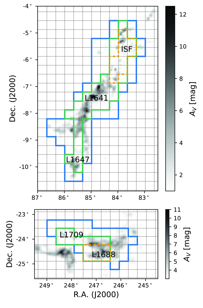
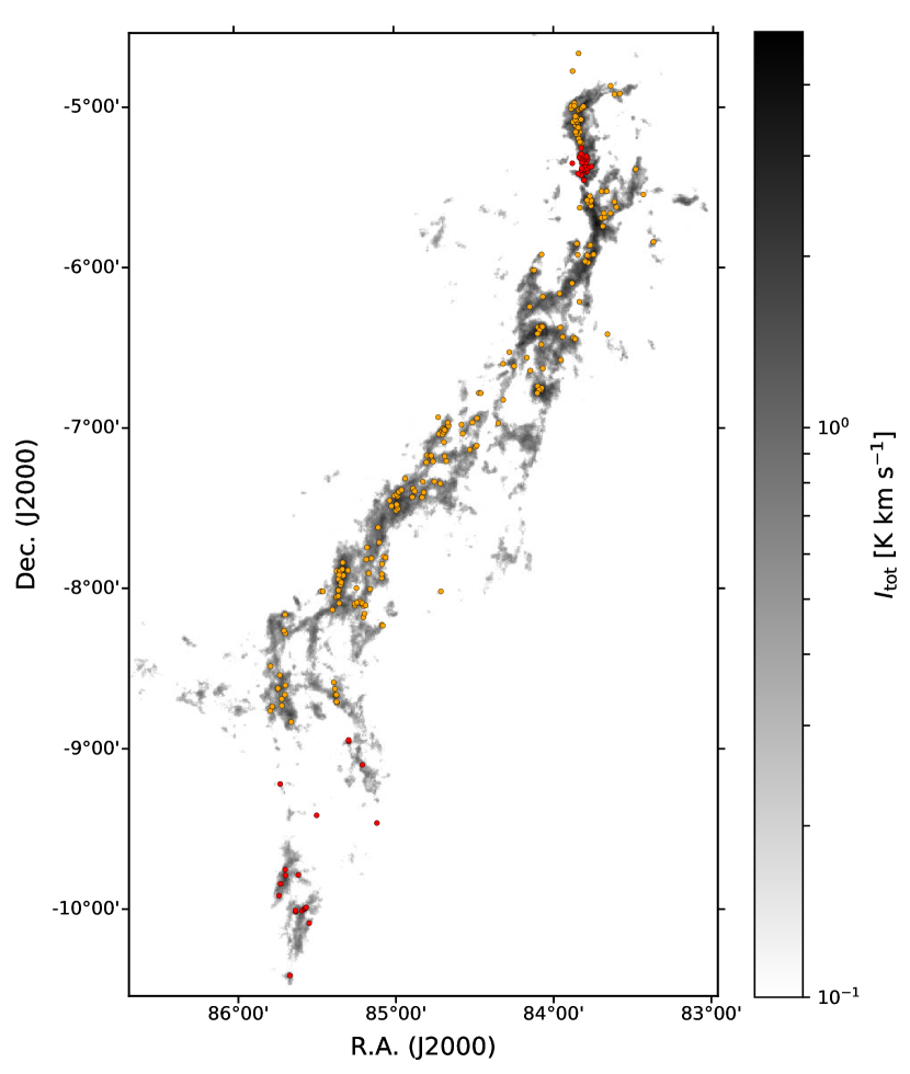
The observed areas toward the Orion A and Ophiuchus clouds are presented in Figure 1. The 13CO/C18O and HCN/HCO+ lines were mapped within the same area through the entire clouds. We obtained the visual extinction () maps provided by Dobashi et al. (2005) and selected initially the submaps, which have higher than a certain value. We adopted of 2.0 and 4.0 for the Orion A and Ophiuchus clouds, respectively, which reasonably outline the structures of the clouds. The OTF observation was initially performed toward the selected submaps, and subsequently, we extended the observation if the 13CO line had been significantly detected on the boundary of the observed area. Total mapped areas in the 13CO/C18O and HCN/HCO+ lines are 8.7 deg2 of the Orion A and 3.9 deg2 of Ophiuchus clouds. For the N2H+/CS lines, observations were made toward the submaps where the observed C18O map exhibits clump-like structures. The mapped areas are 4.0 deg2 and 1.6 deg2 in the Orion A and Ophiuchus clouds, respectively. We observed the N2H+/CS lines deeper than the other lines because of their weak line intensities. Moreover, we chose representative star-forming regions for each cloud: the selected regions are the ISF and L1641-N cluster in the Orion A cloud and the L1688 region in the Ophiuchus cloud. For these regions, we observed the N2H+/CS lines even deeper to obtain high-sensitivity spectral maps. The boundaries of the mapped areas are marked in Figure 1. The total observed time to obtain all data was about 1672 hours; 1073 hours for the Orion A and 549 hours for the Ophiuchus clouds.
The obtained maps were processed using the OTFTOOL and GILDAS/CLASS 111http://www.iram.fr/IRAMFR/GILDAS programs with a cell size of and of about 0.1 km s-1. Baselines were removed using a least fitting method with a first-order polynomial. The baseline fitting is performed for the line-free spectra in the velocity ranges which are outside of the velocity windows (). To obtain good baseline, regions in velocity space () that are almost three times broader than are used. Some of the observed lines show broad wing structures toward OMC-1 where the energetic out-flowing source Orion KL is located (see Section 4.2.1). For these line spectra, we applied velocity windows broader than of the other locations in the cloud. The and values for each spectral map are listed in Table 2.
3 Moment Maps with a Moment Masking Method
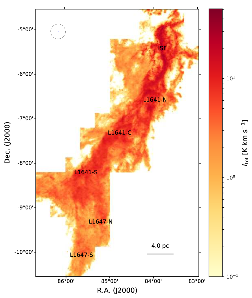
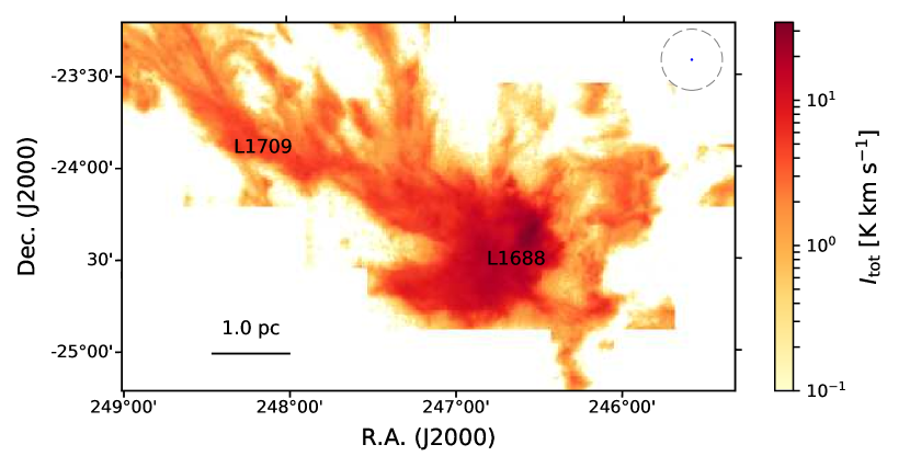
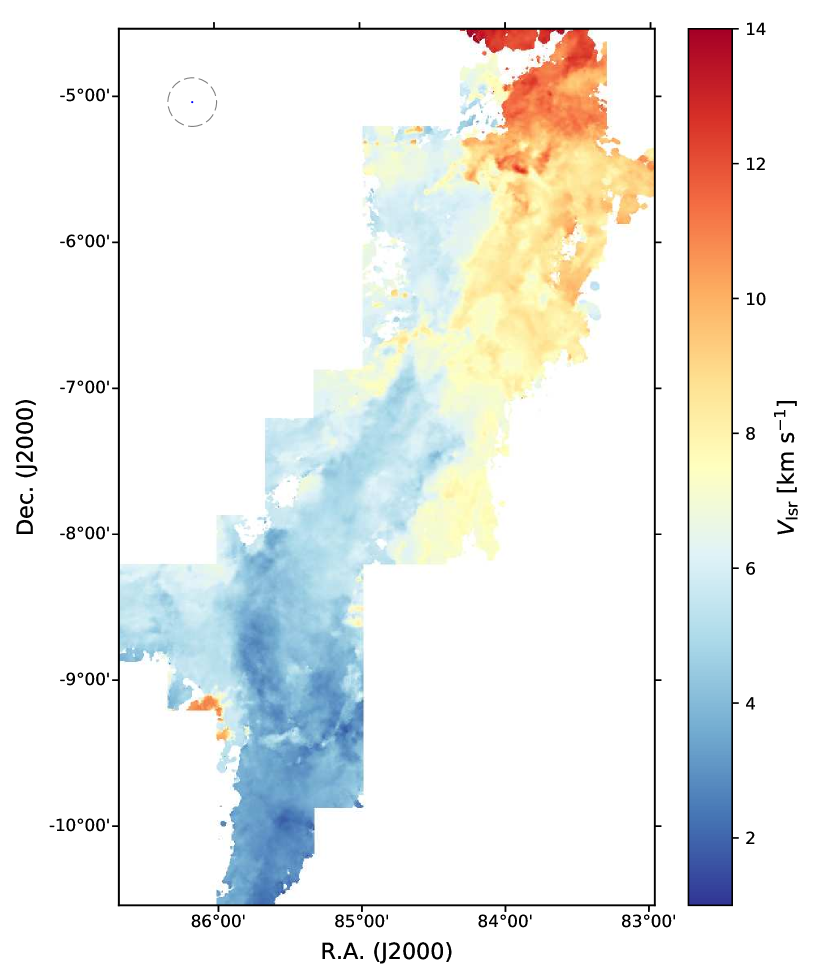
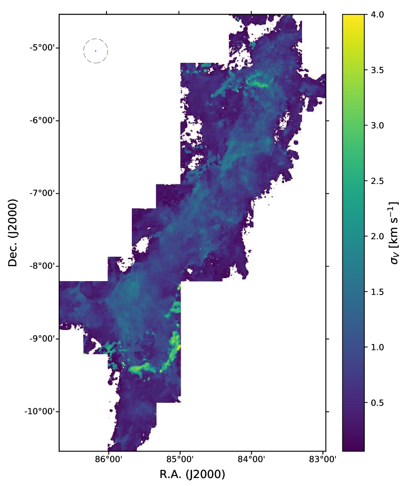
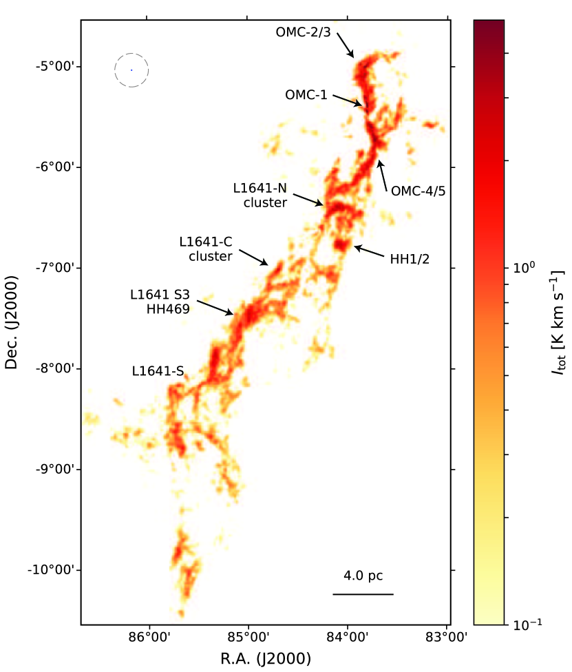
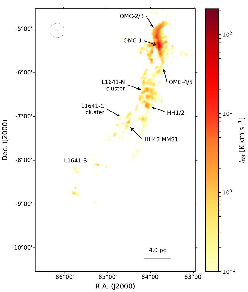
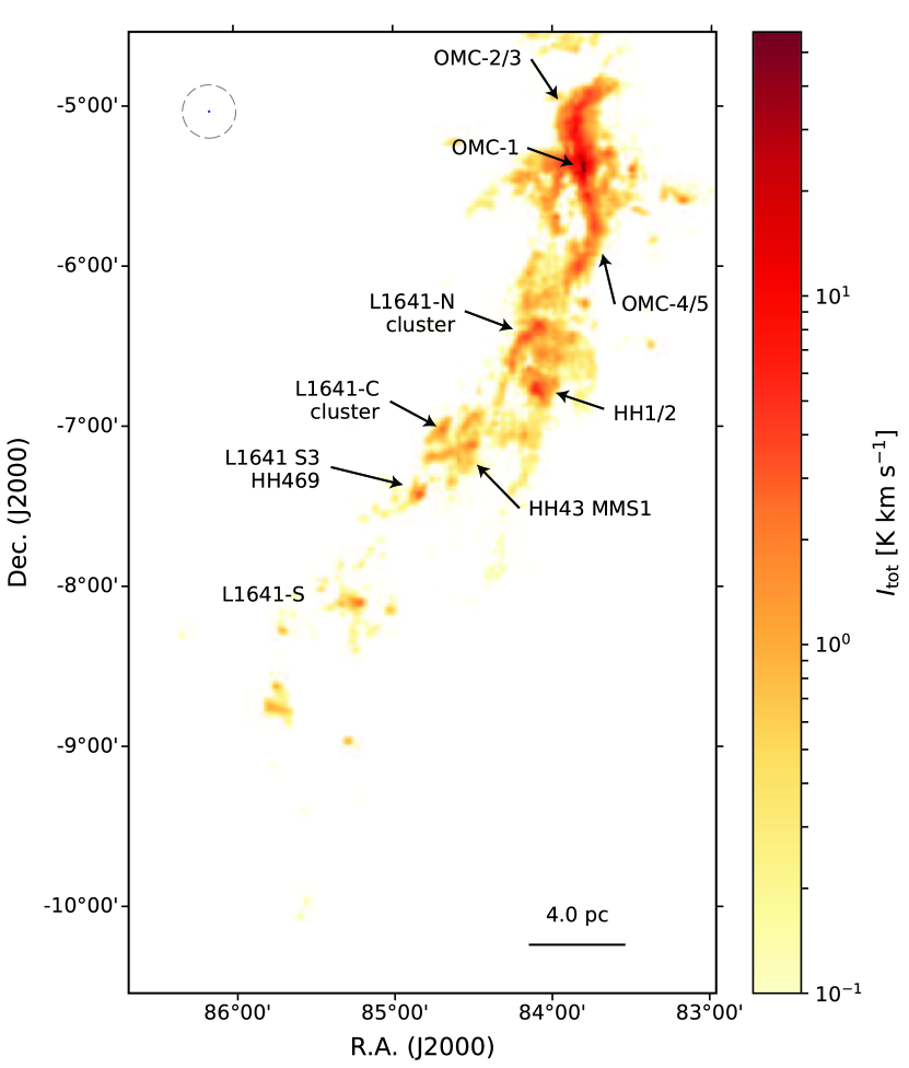
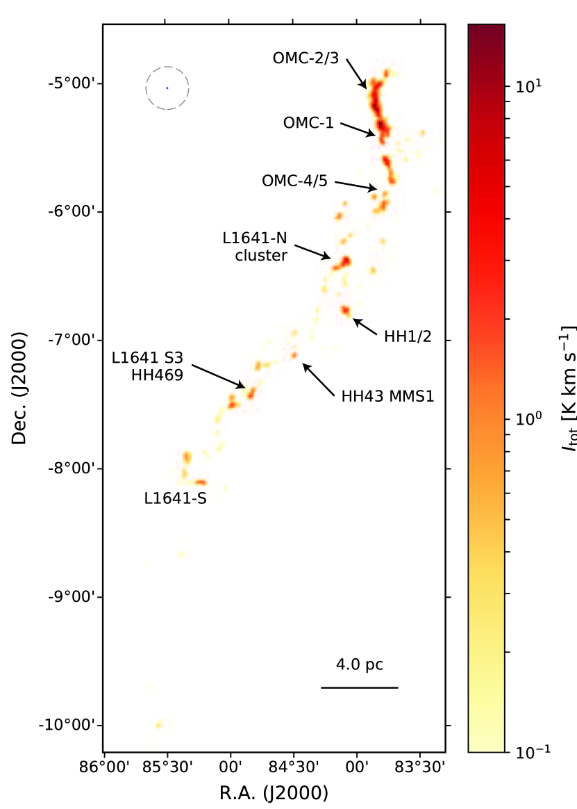
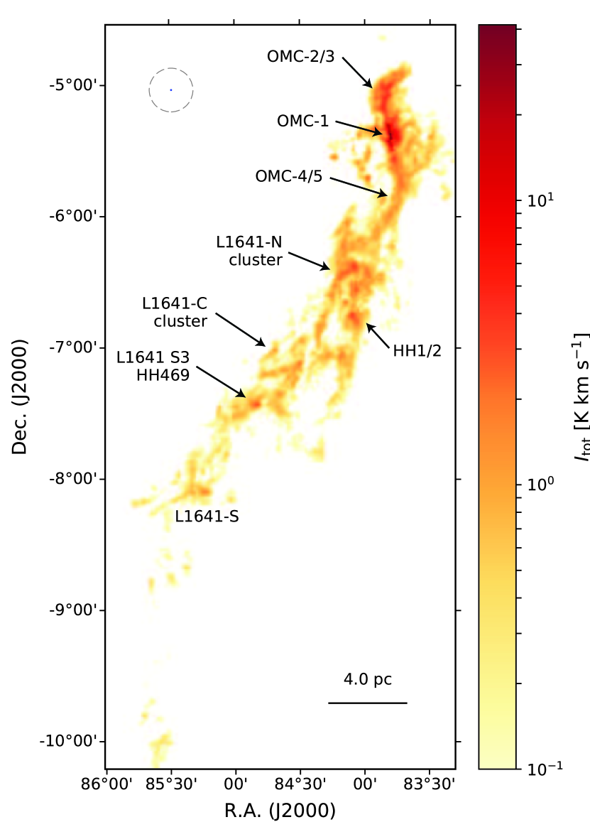
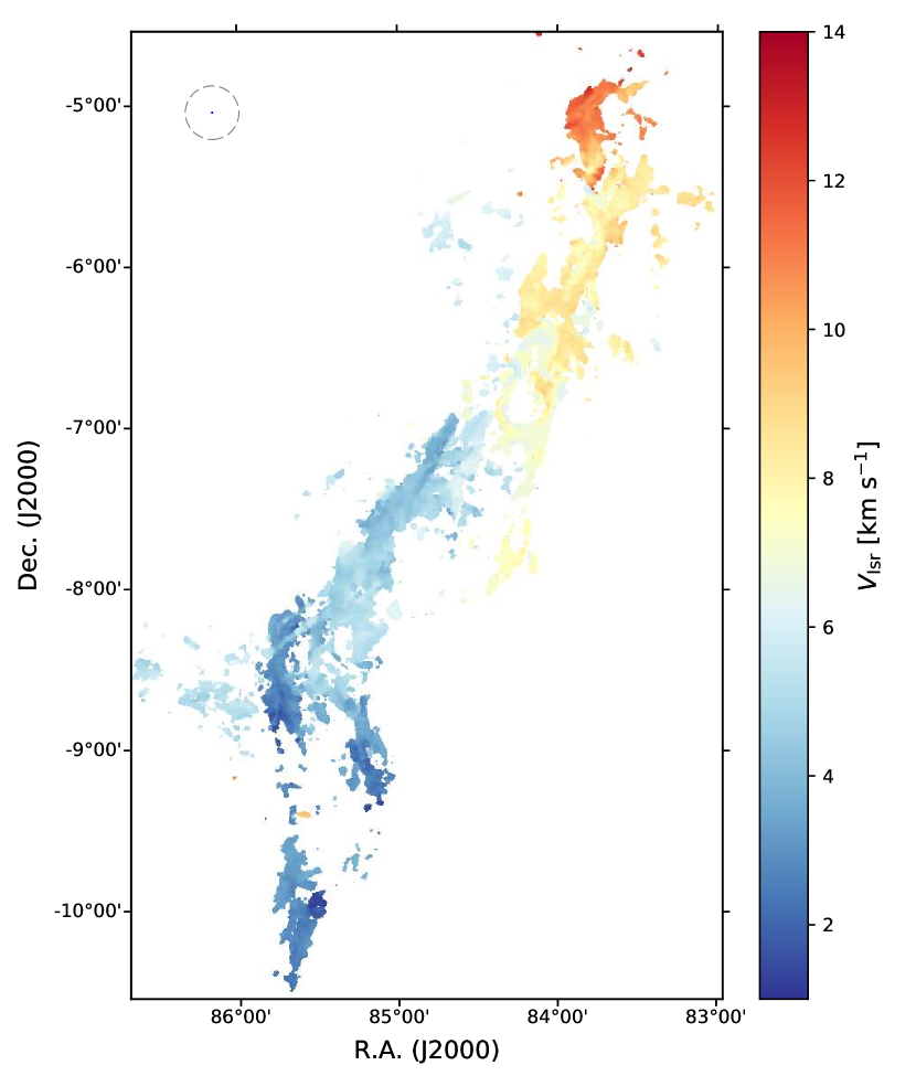
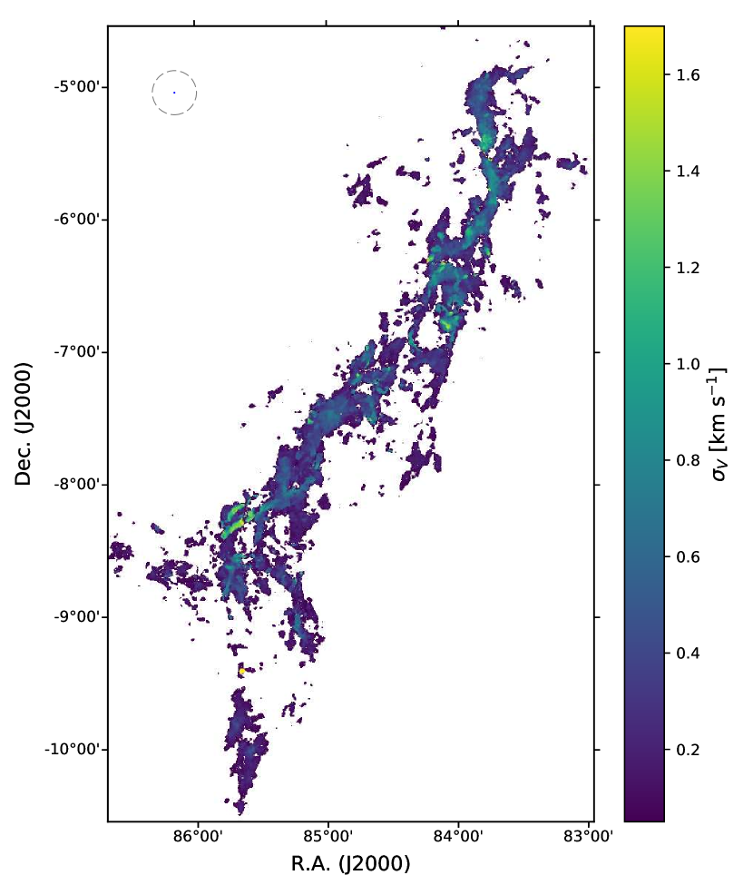
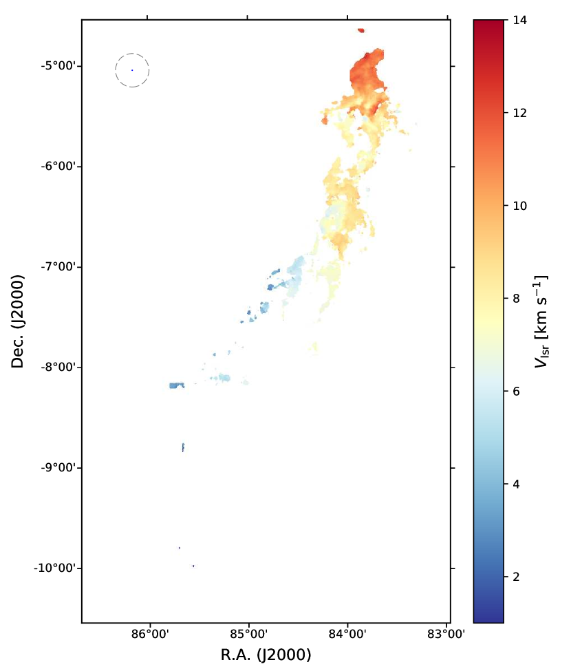
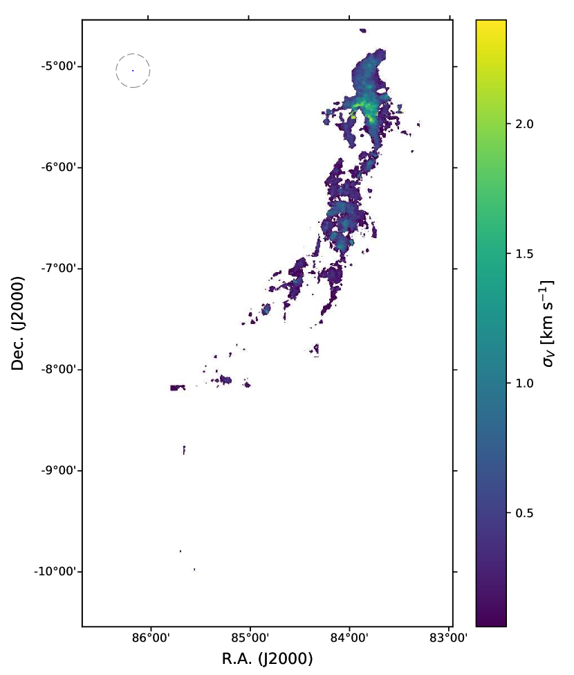
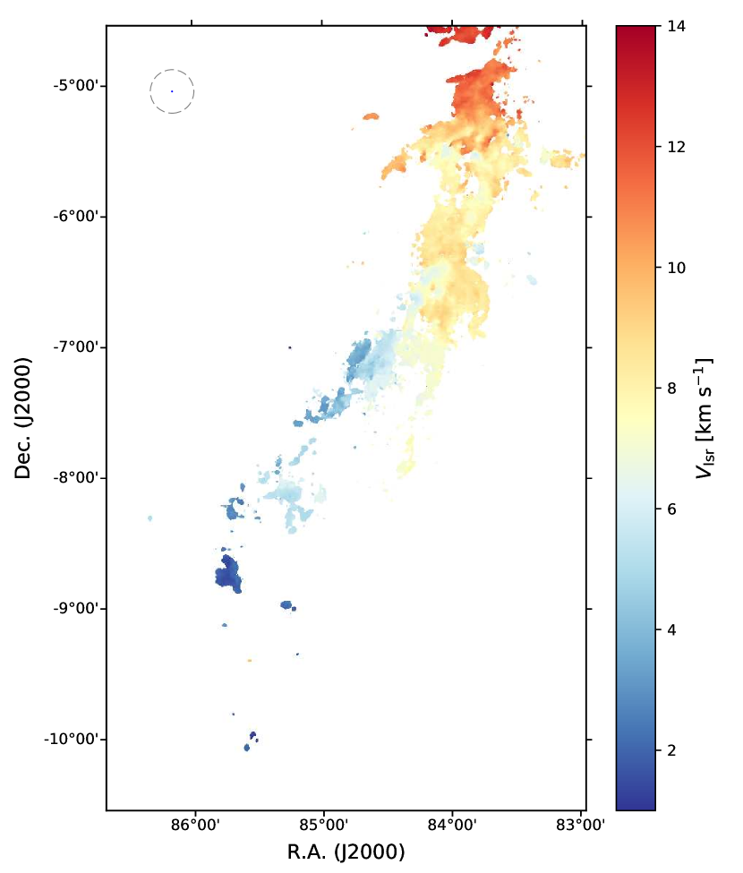
We produced the moment 0, 1, and 2 maps for the observed lines which are equivalent to the maps of integrated intensity (), intensity weighted mean velocity (), and velocity dispersion (). In this process, the moment masking method (Dame, 2011) is applied. The moment masking method is an efficient way to avoid the noise effect which degrades the signal-to-noise ratio of the moment maps. This method identifies emission-free pixels from the smoothed data and removes noise signals within the spectral cube data. The maps of the 13CO line in the Orion A and Ophiuchus clouds are presented in Figures 2 and 3, respectively. The and maps for the 13CO line of the Orion A cloud are presented in Figures 4 and 5 while those for the Ophiuchus clouds are presented in Figures 6 and 7, respectively. The other moment maps for the Orion A cloud are exhibited in Appendix A, and those for the Ophiuchus cloud are exhibited in Appendix B.
We also calculated the uncertainties of the , , and values (, , and , respectively). The uncertainties were derived via the noise propagation. We measured from the line-free spectra of the regions outside and adopted it as an uncertainty of the line intensity. The , , and values are generally dominated by and the number of channels that are included in calculation. The contributions of the velocity uncertainty is minor compared to the other contributions.
For the HCN and N2H+ lines which have multiple hyperfine transitions, we consider a single transition line to derive the and correctly. For the HCN line, we adopted the strongest line at 88.631 GHz. We initially assumed that of the 88.631 GHz line is the same as that of the CS line (). The moment values are derived from the velocity range between 4 and + 3 km s-1, which separate the hyperfine transitions of HCN. The hyperfine transitions of the HCN line are generally blended in the ISF, therefore in the ISF region would be underestimated. For the N2H+ line, we adopted an isolated transition at 93.176 GHz and derived the moment values from 10.87 to + 4.87 km s-1. Finally, we added 7.87 km s-1, which is the velocity difference between the rest frequency and the isolated hyperfine transition, to the derived .
4 Results
4.1 Homogeneous Data Quality
One way to obtain the properties of turbulence from spectral cube data is by statistical analyses, such as the probability distribution functions, two- or three-dimensional power spectra, and a wavelet transform of density or velocity fields (Gill & Henriksen, 1990; Klessen, 2000; Ossenkopf & Mac Low, 2002; Kowal et al., 2007; Burkhart et al., 2009; Koch et al., 2017). For some of these statistical analyses, it is quite important to have well characterized uncertainties, so we focus here on the data uniformity.
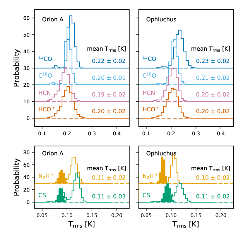
Figure 8 displays the probability distribution functions (PDFs) of . The PDF for each of the 13CO, C18O, HCN, and HCO+ lines have a well-defined single Gaussian-like distribution. The mean and standard deviation of are given in Figure 8. For the N2H+ and CS lines, the PDFs of the N2H+ and CS lines have a pair of Gaussian-like components because of the high-sensitivity maps toward the selected star-forming regions. The filled histograms on the bottom panel are the PDFs for the high-sensitivity maps. The mean values for the N2H+ and CS lines range from 0.10 to 0.11 K, and their standard deviations are less than 0.025 K. For the selected star-forming regions, the means and standard deviations of are 0.09 and 0.006 K, respectively.
These small standard deviation values imply a homogeneous in the spectral maps. The 13CO, C18O, HCN, and HCO+ data have similar mean values, and each of them has a uniform distribution across the observed area. Also, the PDFs of for the N2H+ and CS data imply that does not significantly vary within each of the selected star-forming regions and the other areas.
4.2 The Morphological and Kinematical Features of the Clouds
4.2.1 The Orion A Cloud
In the Orion A cloud, spatial distributions of the observed lines are generally well correlated. All the lines follow a filamentary structure extending from the north to the south (from ISF to L1647-S). The in all lines are generally strong in ISF (Dec. 6.2). Otherwise, all the lines in the southern filamentary structure are weaker than those in the ISF. Also the HCN, HCO+, N2H+, and CS lines are not detected in the L1647 region (Dec. 9; see Figure 2, where these various regions are identified).
The observed lines reveal various structures within the Orion A cloud. The C18O, HCN, HCO+, N2H+, and CS lines are detected toward the regions where the of 13CO is strong. Among these lines, the C18O and N2H+ lines show clumpy structures while the CS line shows relatively extended structures across the Orion A cloud. The HCN and HCO+ lines reveal extended filamentary structures in ISF, while they reveal clumpy structures in the other regions.
The spatial distributions of the C18O, HCN, HCO+, N2H+, and CS lines are well correlated with that of young embedded protostars (Class 0/I young stellar objects and flat-spectrum sources) identified using Spitzer (Megeath et al., 2012) and Herschel observations (Furlan et al., 2016). Especially, the C18O line presents a tight correlation between the spatial distribution of and the embedded protostars (Figure 9). Also, the HCN, HCO+, and CS lines exhibit a similar spatial distribution (Figures A.2. A.3, and A.5). These lines are mainly found in the active star-forming regions (ISF and star-forming clusters) and Herbig-Haro objects (HH1, HH2, and HH43).
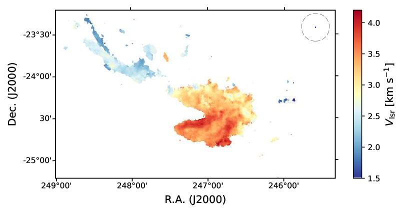
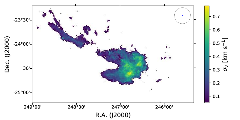
Figures 4 and 5 present the and maps of the 13CO line in the Orion A cloud. The map of the Orion A cloud exhibits a global velocity gradient from the north to the south (Heyer et al., 1992; Tatematsu et al., 1993; Ikeda et al., 2007; Shimajiri et al., 2011; Kong et al., 2018). This global velocity gradient seems to be the motion of the overall Orion A cloud and could represent large-scale rotation (Bally et al., 1987), expansion (Kutner et al., 1977; Maddalena et al., 1986), or gravitational collapse (Hartmann & Burkert, 2007). Statistical analyses without considering the overall motion of MC can cause misunderstanding of turbulence. Therefore, we should take the motion of the Orion A cloud into account when investigating the properties of turbulence in future studies. The ranges from 0.2 to 2.0 km s-1 throughout the Orion A cloud except for some regions with the high- values. These regions are located in the eastern part of ISF and the L1647-N region. In these regions, there are multiple cloud components with different . We will discuss these high- regions in Appendix C.
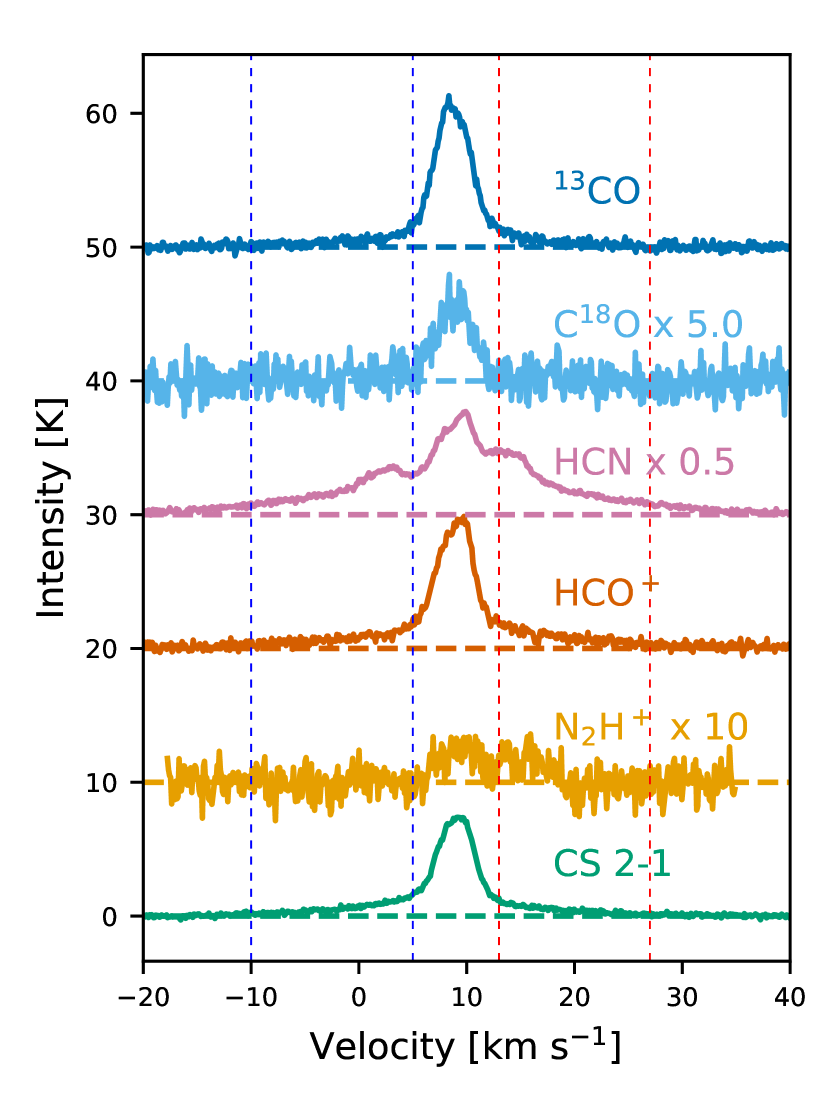
Another notable feature is a broad wing structure in the observed lines toward OMC-1 (Kuiper et al., 1980; Rydbeck et al., 1981; Olofsson et al., 1982; Hasegawa et al., 1984). The 13CO, HCN, HCO+, and CS lines present the blue and red shifted broad wing structures (see Figure 10). For the HCN, HCO+ and CS lines, the broad wing structures result in very high values: the toward OMC-1 are 241, 71, and 51 K km s-1 in the HCN, HCO+, and CS lines, respectively. The values for the HCO+ and CS lines are also high near OMC-1, while the value for the HCN line is not significantly high because of the limited velocity range that we adopted.
The C18O and N2H+ lines do not present clear wing structures in their spectra toward OMC-1. We compared the integrated intensities of the central peak () and the broad wing structures () to check whether or not the weak broad structures exist in the C18O and N2H+ lines. The velocity ranges that and are derived over are summarized in Table 3. The observed lines generally peak at the velocity of 9 km s-1. We thus derived over a velocity range from 5 to 13 km s-1 assuming that the central peak extends up to 4 km s-1 from the line center. was calculated over the velocity ranges from -11 to 5 and from 13 to 29 km s-1 assuming that the wings extend up to 20 km s-1 from the line center. For the HCN and N2H+ lines, the velocity ranges for obtaining were set to cover all hyperfine components. Also, we set the velocity ranges of the wing structures to consider the broad emission features at the outermost parts of the observed lines.
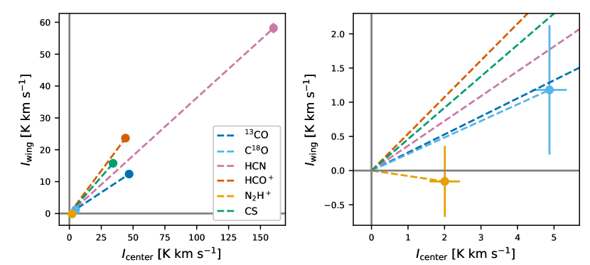
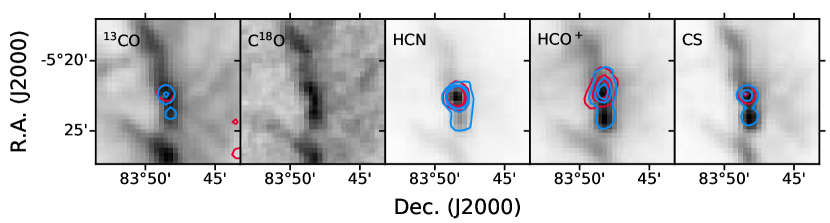
Figure 11 presents the and for each line. values are generally proportional to . The 13CO, HCN, HCO+, and CS lines have relatively strong values that are higher than 10 K km s-1. of C18O is barely detected (1.1 0.3 K km s-1). Only the N2H+ line is not detected with a value of 0.16 0.17 K km s-1. Figure 12 presents the distributions of the broad wing emission in 13CO, C18O, HCN, HCO+ and CS. Note that the distribution of wing emission in C18O is indistinguishable from the noise.
4.2.2 The Ophiuchus Cloud
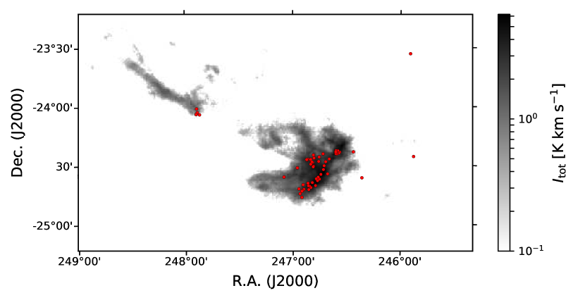
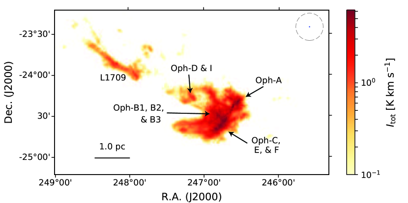
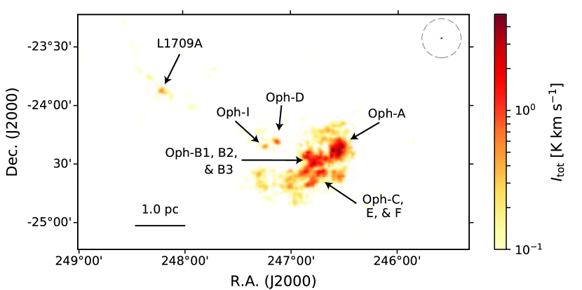
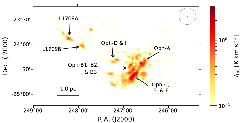
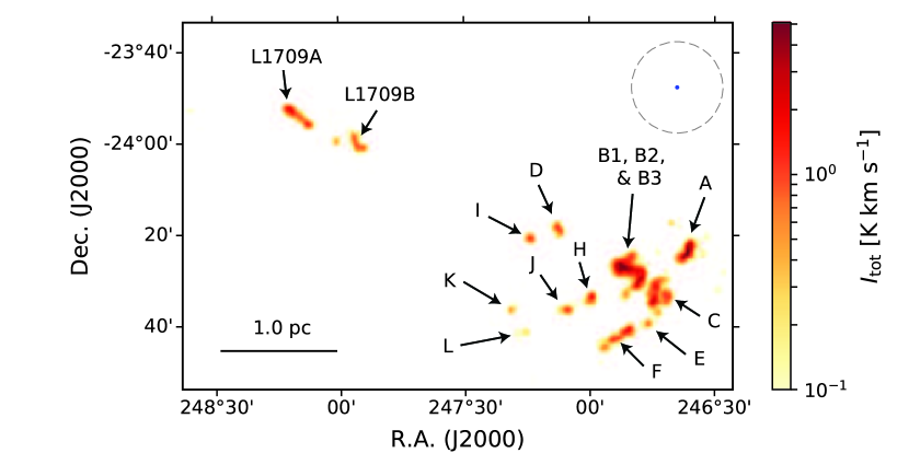
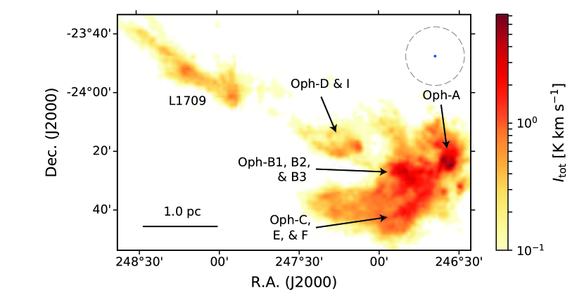
In the Ophiuchus cloud, the observed lines exhibit spatial distribution trends that are similar to those in the Orion A cloud. The 13CO line traces extended cloud structures from the L1688 to L1709 regions (the regions of the cloud are identified in Figure 3). The other lines mainly trace small and clumpy structures in the cloud. The line intensities are generally strong in L1688 (R.A. 247.5), which is the most active star-forming region in this cloud. Also, the spatial distribution of the C18O line emission is well correlated with that of the young embedded protostars identified using Spitzer (Dunham et al., 2015, see Figure 13).
In L1688, the observed lines are generally strong toward the star-forming cores (Oph-A through L; see Figure B.4). But, their relative strengths change depending on the lines. The star-forming cores have non-uniform conditions (Pattle et al., 2015; Punanova et al., 2016). Oph-A and -C are affected by the external heating from the B2V star HD 147889 (Pattle et al., 2015; Punanova et al., 2016). Oph-B1 and -B2 cores are the coldest among the cores (Pattle et al., 2015); Oph-B1 is one of the quiescent cores while Oph-B2 is the most turbulent core (Punanova et al., 2016). Oph-E and -F cores are the most evolved regions in L1688 (Pattle et al., 2015); Oph-E is strongly pressure-confined while Oph-F is marginally pressure-confined. Also, Oph-F has a similar temperature to that of Oph-A without any external heating. These different environments result in the different relative strength of the observed lines.
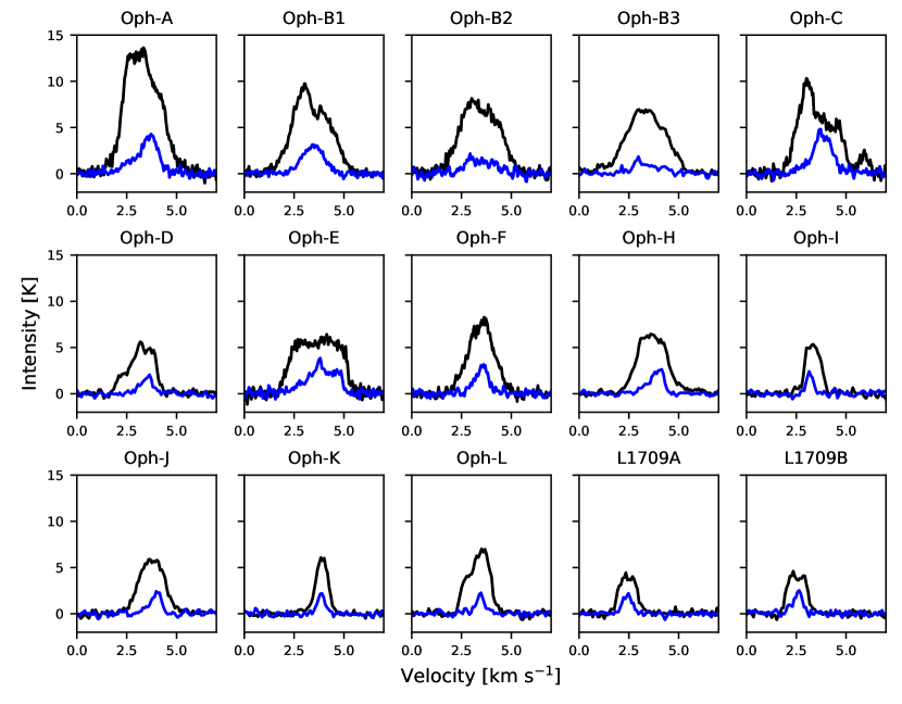
The of the 13CO line in Oph-A is stronger than that in Oph-C while that of C18O in Oph-A is similar to that in Oph-C. Lada & Wilking (1980) found that 13CO 10 is optically thick with a self-absorption feature in some positions. We thus investigated the 13CO and C18O lines toward the dense cores where the 13CO line can probably be optically thick. Figure 14 presents the 13CO and C18O line spectra toward the 13 cores in L1688 (Pan et al., 2017) and two DCO+ cores in L1709 (Loren et al., 1990). Some of the dense cores present self-absorption features in their 13CO line spectra.
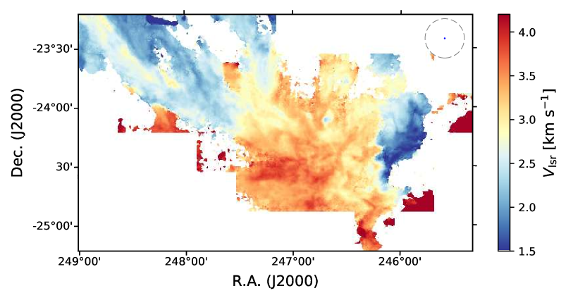
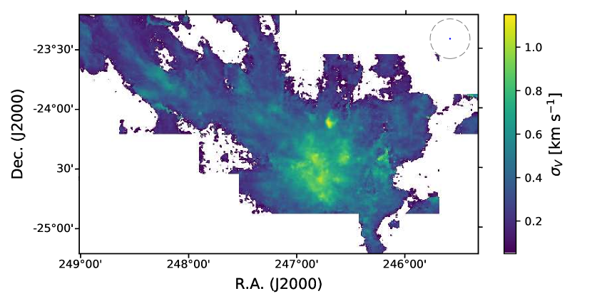
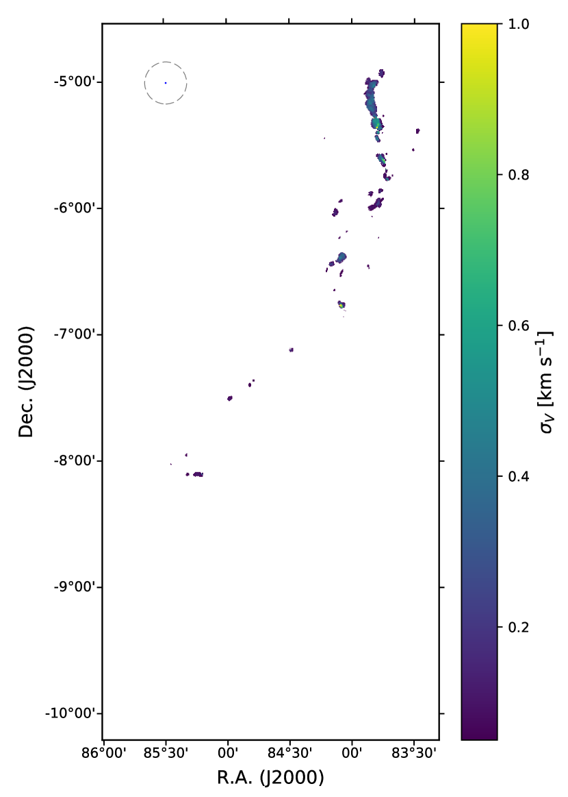
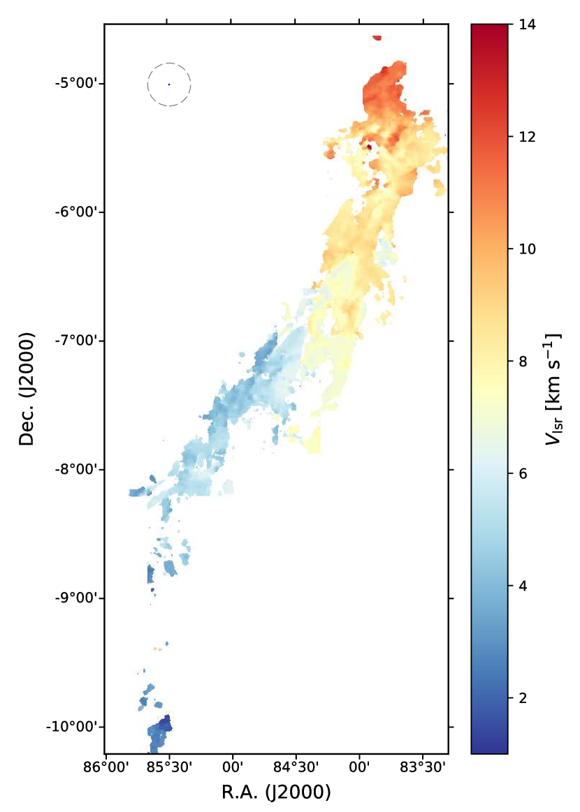
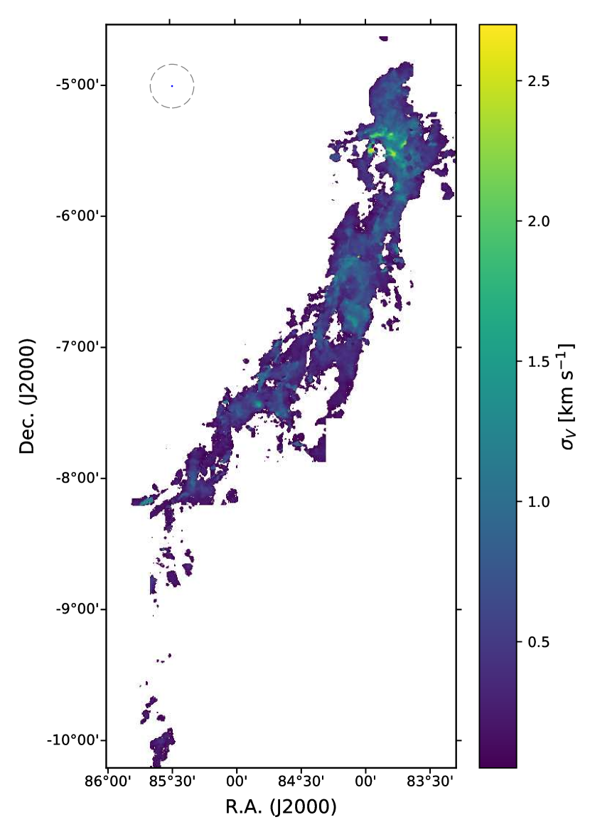
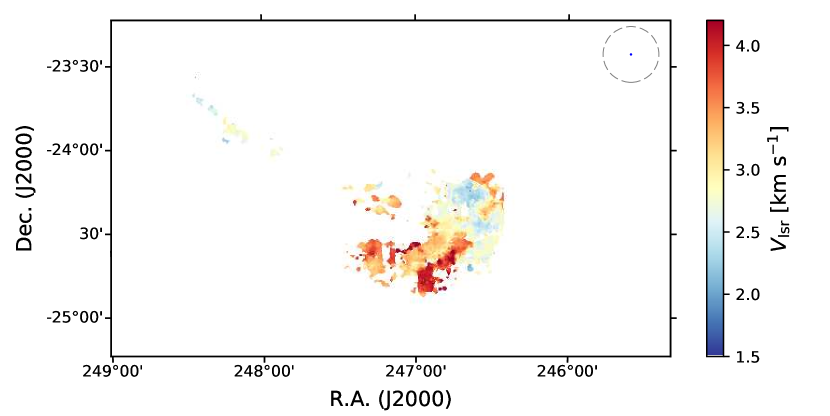
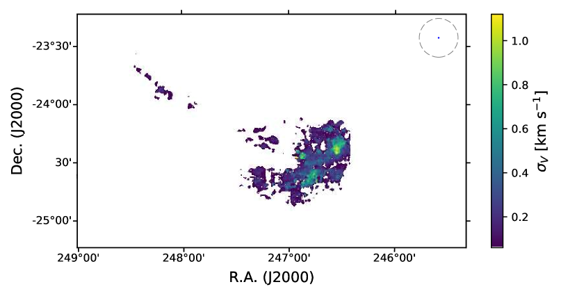
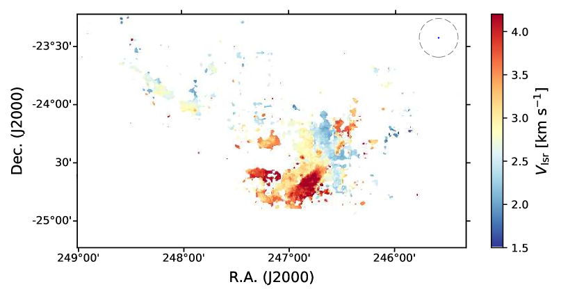
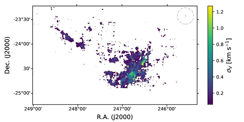
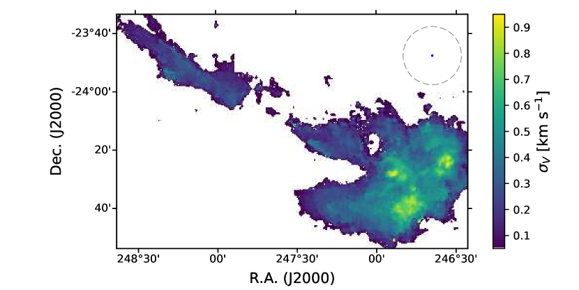
Figures 6 and 7 show the and maps for the 13CO line in the Ophiuchus cloud. The value varies from 1.5 to 4.0 km s-1 across the Ophiuchus cloud. The map shows that the L1688 and L1709 regions have different . The values of L1688 are around 3.5 km s-1 while that in L1709 is around 2.5 km s-1. From this result, Loren (1989b) suggested that L1709 may be separate from L1688. Neither L1688 nor L1709 regions have any overall motions in the 13CO line. We also checked the optically thinner C18O line, but there is no overall motion in each region (see Appendix D). The is about 0.5 km s-1 across the Ophiuchus cloud.
The moment maps of the 13CO line imply that the kinematic features of the Ophiuchus cloud are quite different from those of the Orion A cloud. The systematic variation of the in the Ophiuchus cloud is relatively small compared to that in the Orion A cloud. Also, the typical value in the Ophiuchus cloud is smaller than that in the Orion A cloud. The small variation of and small values imply that the Ophiuchus cloud is kinematically quiescent compared to the Orion A cloud (Loren, 1989b).
The difference between the spatial distributions of the HCN and HCO+ lines is striking (see Figures B.2 and B.3). The HCN line is mainly detected toward Oph-A, -B1, -B2, and -B3 cores while the HCO+ line is predominantly detected toward Oph-A, -C, -E, and -F cores. The peak of the HCN and HCO+ lines also appear in different cores. This result indicates that the HCN and HCO+ lines trace different physical or chemical conditions in the Ophiuchus cloud.
4.3 Column Density Maps and Variations with Column Density
Unbiased mapping toward two MCs in multiple molecular lines provides a good opportunity to assess how the line intensities respond to the physical parameters within clouds. Therefore, we investigated the variation of as a function of column density ().
We derived from the observations of dust continuum emission that can trace the amount of gas in a cloud (Goodman et al., 2009). The maps were derived by fitting a modified blackbody (MBB) into the spectral energy distribution (SED) of the continuum emission from cold dust. Archival Herschel PACS (160 m) and SPIRE (250, 350, and 500 m) continuum observations that were obtained as part of the Herschel Gould Belt Survey (André et al., 2010) are adopted. Note that the PACS 100 and 70 m observations are not included in the SED fitting. The 100 m continuum observation was not covered by the Herschel Gould Belt Survey (André et al., 2010). For the 70 m band, the MBB fitting with a single temperature cannot fit the observed emission in some cases because of the contamination due to non-equilibrium emission from small dust grains (Roy et al., 2013). Even if the detailed dust model is applied to the SED fitting including the 70 m data, the derived column density is not significantly different from that derived using the single temperature MBB fitting without the 70 m data (Bianchi, 2013).
The continuum emission maps were calibrated using Planck observations of the same regions via the method in Chen et al. (2019). Using the calibrated data, the column density maps were derived in two steps (Friesen et al., 2017; Chen et al., 2019): (1) dust temperature () and optical depth () maps were found via the SED fitting, and (2) the maps were obtained from the map by multiplying by a conversion factor assuming a gas-to-dust mass ratio of 100,
| (1) |
where is the opacity of 0.1 cm2 g-1 at of 1000 GHz (Hildebrand, 1983), is a mean molecular weight per H2 molecule of 2.8, and is the mass of a hydrogen atom. The final map has a beam size of 36, which is the resolution of the SPIRE 500 m data. We thus convolved the map to have a resolution of 50, which is comparable to the beam sizes of the TRAO maps (see Table 1).
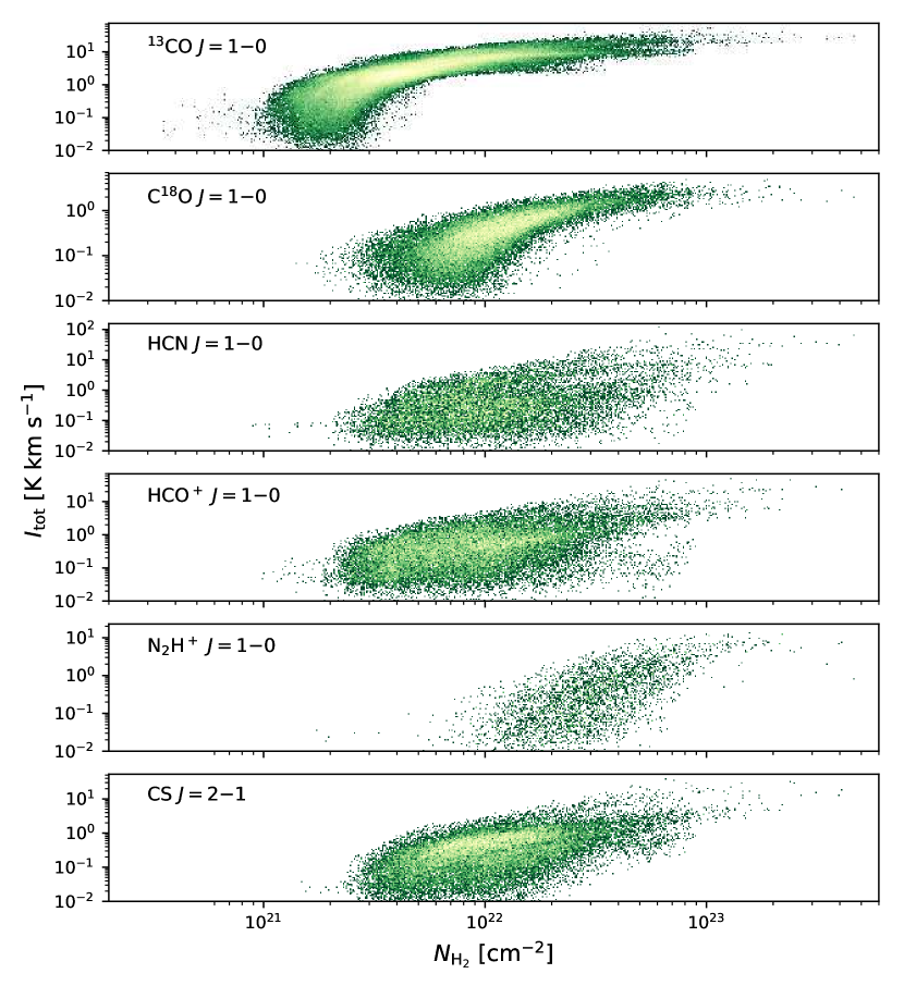
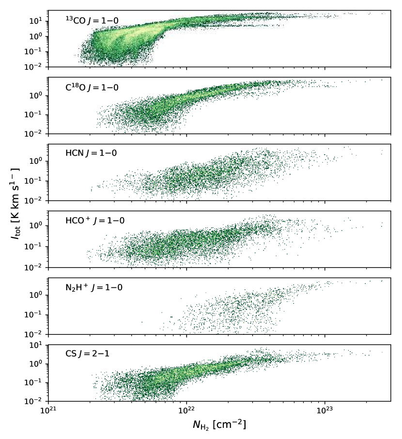
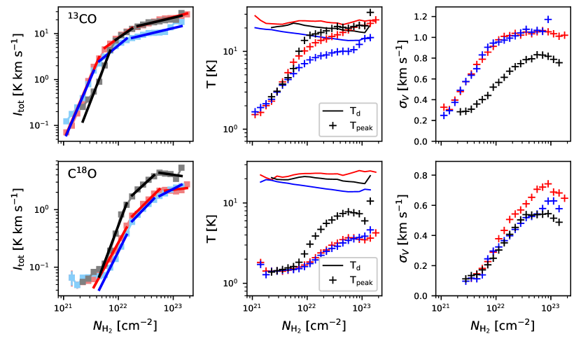
The of each observed line generally increases as increases up to a certain and remains relatively constant after that certain (see Figures 15 and 16 for the Orion A and Ophiuchus clouds, respectively). We fit the variation with a power-law relation to characterize how of a molecular line changes as increases. In this process, we divide the Orion A cloud into two sub-regions, the ISF region (Dec. ) and the rest of the cloud (Dec. ) because ISF is more likely to be affected by the PDR (Shimajiri et al., 2014). Hereafter, ISF, the other regions in the Orion A cloud, and the Ophiuchus cloud are referred as the ISF, L1641, and Ophiuchus regions.
For each line in each of the ISF, L1641, and Ophiuchus regions, the mean values of the , peak temperature (), , and for a given are investigated. The line spectra were separated into regularly spaced -bins with a size of 0.1. We derived the mean values of and for each bin, weighting the values by the inverse of the square of the uncertainty. For the and , the arithmetic mean values are adopted. Note that the variation of seems to be relatively constant because it generally varies from 12 to 20 K in most areas except near the heating sources (such as OMC-1 and NGC 1977 in the Orion A cloud and HD147889 in the Ophiuchus cloud).
We investigated the power-law indices which can explain the variation of the mean values (). We fitted the data with a power law: . The minimization technique was used to obtain the fit parameters. The value is defined as follows,
| (2) |
where the sum is over the bin numbers, is an expected value from the power-law fit, and is the uncertainty of . For C18O, HCN, HCO+, N2H+, and CS, there are several data points with very weak and relatively constant at a low- regime ( 21021 cm-2). These data points are the weighted means of a few pixels. Their line spectra are generally dominated by the noise although the moment masking method identified them as emission lines. Therefore, we excluded these data points from the power-law fitting. The ranges for power-law fits were visually defined. The ranges for the fitting and the best-fit power-law indices () are listed in Table 4.
Figure 17 shows the variation of the 13CO and C18O lines. For these lines, we divided the range into three regimes: (1) the low- regime where steeply increase ( 2.0), (2) the intermediate- regime where is proportional to ( 1.0), and (3) the high- regime where becomes relatively constant ( 1.0). The detailed ranges are different depending on the lines and regions, however, their variations are similar.
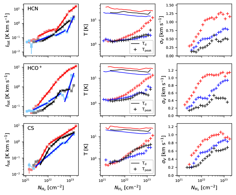
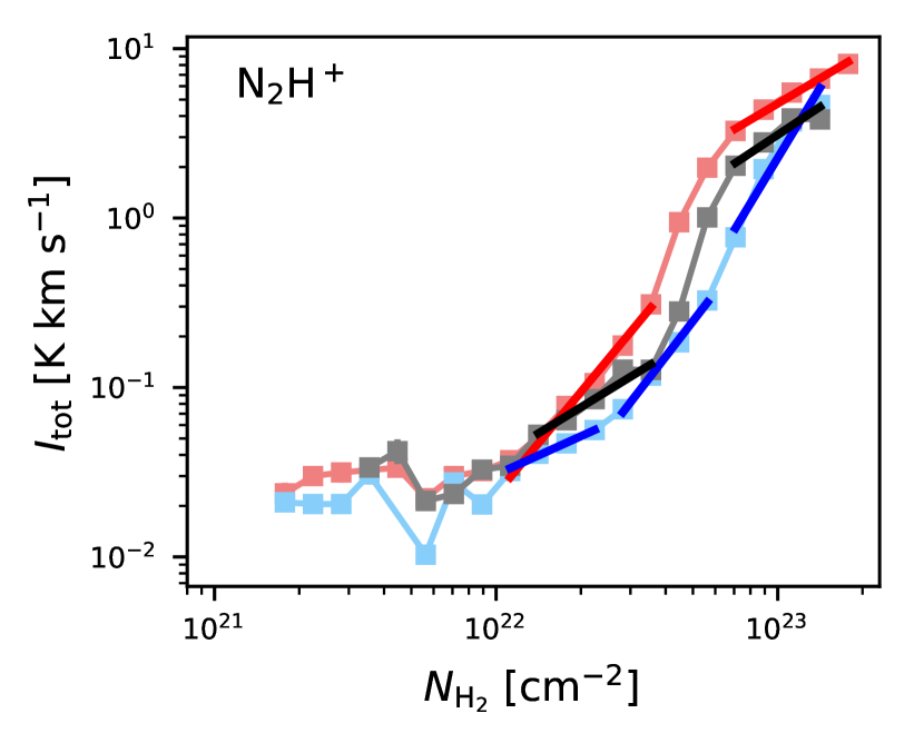
Figure 18 shows the variations in HCN, HCO+, and CS lines. The variations of are quite different depending on the lines and regions and cannot be explained with a single trend. Their variations should be interpreted individually. The variation of the N2H+ line is presented in Figure 19. The N2H+ line is only detected at the high- regions where is higher than 1022 cm-2. We will discuss these results in Sections 5.2 and 5.3.
5 Discussion
5.1 Broad Wing Structures in the Orion KL Spectra
As noted above, the Orion-KL region shows wide line wings in 13CO, HCN, HCO+, and CS, marginally in C18O, and not in N2H+. Wannier & Phillips (1977) suggested that 12CO J=1-0 is optically thin in the wings. The 13CO and C18O lines thus would be optically thinner at the line wings. In this case, the intensity ratio between the 13CO and C18O lines is probably close to their abundance ratio (Wannier & Phillips, 1977). The ratio between of the 13CO and C18O lines is 10.5 2.8. This value is close to the abundance ratio determine by Shimajiri et al. (2014) ( = 12.14) within a 1- range.
The ratios between and for the HCN, HCO+ and CS lines are slightly different. The origins of the broad wing structures were discussed in previous works (Kuiper et al., 1980; Rydbeck et al., 1981; Olofsson et al., 1982; Hasegawa et al., 1984). The bipolar outflows aligned with the line of sight are suggested as the origin of the high velocity wings (Olofsson et al., 1982). In this case, the high velocity emission is spatially confined close to Orion KL. For the HCO+ line, the contribution of the shocked gas is also suggested (Rydbeck et al., 1981; Johansson et al., 1984; Olofsson et al., 1982). In addition, the abundance enhancement of HCN and HCO+ in the high velocity components is also reported (Rydbeck et al., 1981; Johansson et al., 1984). Hasegawa et al. (1984) analyzed the CS line and suggested that the existence of a large gas disk around Orion KL nebula. They also mentioned that the high velocity emission corresponding to the bipolar outflows was not observed in CS. These results may be related to the differences in ratios between and .
5.2 Variation of as a Function of
If all the following assumptions are true (the lines are optically thin, stimulated radiative processes can be ignored, excitation temperatures are much lower than the kinetic temperature (), and the abundance of the species is constant), the line intensity is proportional to because every collision leads to a photon. If the line of sight depth is constant, the line intensity is also proportional to , as is generally true for optical or infrared emission lines. All these conditions are rarely met for millimeter-wave molecular emission lines. The fact that the excitation temperature is limited below by the radiation temperature and above by the kinetic temperature constrains the regime of densities over which every collision leads to a photon. Optical depth increasing with also leads intensity to increase more slowly with . For lines that reach optical depth near unity and excitation temperatures near the kinetic temperature, the intensity should plateau with . The dependence of on is a complicated function of density, temperature, abundance, and velocity field.
Examination of Figures 17 and 18 and the fits in Table 4 show broad agreement with these predictions. At low , the fits to intensity versus are super-linear, but they become closer to linear at higher before reaching plateaus at levels that depend on . The middle plots of Figures 17 and 18 show and from Herschel. For densities above a few times 104 cm-3, . For 13CO, indeed levels off near , as predicted for optically thick, thermalized lines. None of the other transitions reach this point, so the fits to their slopes indicate that they lie primarily in the intermediate zone between growing like and the plateau. N2H+ is the exception, with slope near the predicted value of 2 over a substantial range of in the ISF, where is relatively high.
Kauffmann et al. (2017) analyzed the 13CO, C18O, HCN, and N2H+ lines in the northern part of ISF and presented the normalized line-to-mass ratio as a function of the visual extinction () derived from Herschel column density. Figure 2 in Kauffmann et al. (2017) showed that there is a certain regime where the line-to-mass ratios remain relatively constant which means that the is proportional to . Table 5 shows the regimes where the line-to-mass ratio remains constant and corresponding values for each line for the lines studied by Kauffmann et al. (2017) and the corresponding values for our study.
For the 13CO, C18O, and N2H+ lines, the regime where of about 1.0 is generally consistent with that from Kauffmann et al. (2017). The regimes for 1.0 that are derived in this study are larger than those of Kauffmann et al. (2017). For the HCN line, the regime is quite different from what Kauffmann et al. (2017) presented. Kauffmann et al. (2017) only adopted a small region north of -5:10:00 Dec. (J2000) to avoid the effect of radiation which is emitted from the Orion Nebula. However, the whole region north of -6:00:00 Dec. (J2000) including OMC-1 is included in this study. The different results for column density regimes might be caused by the difference in the areas that are included in each analysis.
5.2.1 13CO 10
The 13CO line has where cm-2. The uncertainty of in these regimes is larger than that in the other regimes. Thus, detailed interpretation of variation using could be uncertain. The values in intermediate- regimes are close to 1.0 and become shallower in the high- regime ( 0.3). This result indicates that the 13CO lines in both clouds are optically thick toward high- regions and cannot trace all the gas along the line of sight. In the Ophiuchus cloud, self-absorption features appear in the 13CO line spectra toward the star-forming cores. These results are consistent with previous studies showing that 13CO line can be optically thick in the Orion A (Shimajiri et al., 2014) and Ophiuchus (Lada & Wilking, 1980) clouds.
In this analysis, we neglected the effect of abundance variation within MCs. In fact, the variation of the 13CO line also can be affected by the chemical difference between the sub-regions. The ISF region is also affected by the photon-dominated regions (PDRs) heated by the Trapezium stars (Shimajiri et al., 2014). In cold dense regions, 13CO can freeze onto dust grains.
5.2.2 C18O 10
The observed C18O lines preferentially trace regions of higher column density than are traced by the 13CO line. This is understood as the effect of lower abundance (Wilson & Rood, 1994) which translates into lower optical depth and less radiative trapping. When is smaller than 31022 cm-2, only a few weak emission lines were detected. If we observe both clouds more deeply, the variation in very low regimes would be accessible.
In the intermediate- regime, where is between 1.61022 and 5.01022 cm-2, the values are about one. If exceeds 5.01022 cm-2, the slopes become shallower. In the ISF and Ophiuchus regions, becomes comparable to zero. For the ISF region, Shimajiri et al. (2014) found that C18O 10 is optically thin, and the abundance of C18O would be affected by the selective photodissociation in PDR chemistry. Abundance variations caused by photodissociation or freeze-out (Caselli et al., 1999) can also affect the line emission. In the Ophiuchus region, sharply increases beyond of 1023 cm-2. This increase results from a selection bias; the highest bin originates only from the Oph-A core that has the highest and within the Ophiuchus region.
5.2.3 HCN 10 and HCO+ 10
The for the HCN and HCO+ lines shows different variation depending on the lines and regions. Also, the for a given line and region changes in different ways depending on the regimes. Only the variation for the HCO+ line in the ISF region is similar to what the 13CO and C18O lines exhibited. This difference seen in the HCO+ and HCN lines may be due to different star formation activities in different regions. HCO+ and HCN have been known as good tracers of star-formation activities because they become abundant in the gas affected by shocks and high energy UV photons.
5.2.4 CS 10
The variation of the CS line shows that decreases as increases, similar to what was seen for 13CO and C18O lines. However, the values are generally greater than or similar to one. Only the Ophiuchus cloud has significantly smaller than one ( 0.63) when exceeds 22.6.
Table 4 shows that the variation of CS can be explained with of about 1.0 across the large regime. In the ISF and L1641 regions, the regimes with 1.0 are extended over one order of magnitude. This result indicates that the of CS is proportional to over the broad range of in the Orion A cloud. Pety et al. (2017) also mentioned that CS 21 is one of the more useful column density tracers in the Orion B cloud.
5.2.5 N2H+ 10
The N2H+ line increases super-linearly at low column densities before approaching a more linear growth at higher column densities. This behavior reflects the low abundance of this species in gas of low column density and high CO abundance. It makes it a good probe of gas column density for regions of relatively high column density.
The dominant formation mechanism of N2H+ molecule is
| (3) |
When the CO abundance is close to 104 which is a typical value in MCs (Wilson & Rood, 1994; van Dishoeck et al., 1995), H mainly combines with CO to form HCO+. Also, N2H+ is destroyed by combining with CO,
| (4) |
Therefore, N2H+ line can be abundant in dense gas where CO is depleted from the gas phase (Bergin & Langer, 1997; Aikawa et al., 2001; Lee et al., 2003, 2004; Tatematsu et al., 2008). Therefore, of the N2H+ line represents the column density of the dense gas if we assume that the N2H+ line is optically thin.
The of the N2H+ line is proportional to the amount of cold and dense gas along the line of sight if the N2H+ line is optically thin. The mean value at a given in the ISF region is slightly higher than that of the L1641 and Ophiuchus regions. This result implies that the amount of the dense gas along the line of sight in the ISF region is slightly larger than that in the L1641 and Ophiuchus cloud. Tatematsu et al. (2008) also mentioned that the abundance of N2H+ decreases toward the south in ISF. Therefore, the difference in of N2H+ also can be explained with an abundance difference between the regions.
5.3 Variation of Velocity Dispersion with Column Density
The right-hand panels of Figures 17 and 18 display the RMS velocity dispersion (moment 2; ) versus . The dispersion depends strongly on , increasing by factors of 3-5, depending on the lines and regions. Weak lines can produce unrealistically small values of , but we have tried to avoid that by using the moment masking method to make the map and by adopting the average values weighted by the inverse of the square of the uncertainty. Consequently, we believe that the strong trends in versus are real.
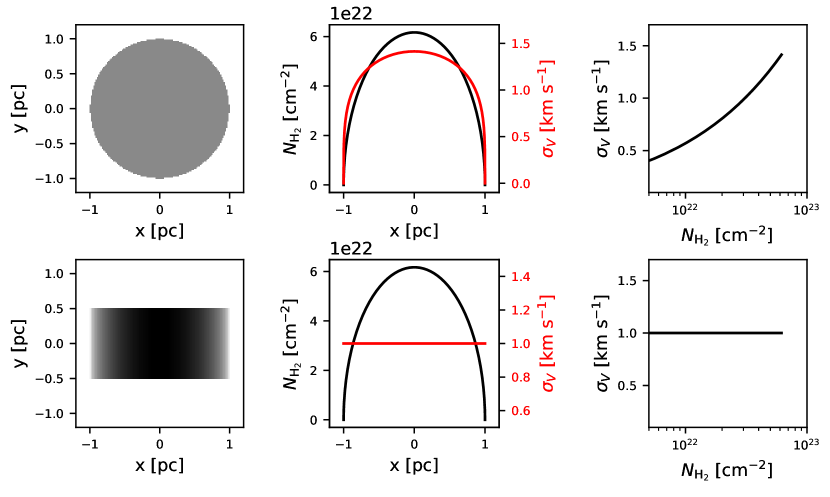
Two simple cloud models can be adopted to describe the increasing toward the center from the outer region: (1) a structure with a varying depth, like a cylinder with a uniform density located along the sky plane, and (2) a structure with a uniform depth, such as a slab with varying density, as illustrated in Figure 20. The observed linewidth is determined by sampling a turbulent velocity field along the line of sight (y-direction). If the linewidth correlates with path length, as expected from the turbulent velocity field (Larson, 1981; Solomon et al., 1987; Heyer & Schloerb, 1997; Klessen, 2000), the increases with in the cylindrical model while that remains constant in the slab-like model. This result suggest that the cylinder cloud model can explain the low- edges of the cloud with low-, unlike the slab-like cloud model.
5.4 Line Luminosities and Luminosity Ratios
The line luminosity of each line in the Orion A and Ophiuchus clouds is calculated by
| (5) |
where , , , are the distance, angular size of a pixel (20″), number of pixels, and line integrated intensity per pixel, respectively. The is defined as
| (6) |
where is the beam size. The distance to the Orion A cloud is assumed to be 416.3 pc, which is the average of the distances to the Orion nebular cluster, L1641, and L1647 (389, 417, and 443 pc, respectively Kounkel et al., 2018). For the Ophiuchus cloud, we adopted 137 pc (Ortiz-León et al., 2017).
The value of requires discussion. We have done the summation in two ways. In the first, only the pixels that in the moment-masked map of each line were included. Very weak emission extended over large areas can however contribute substantially to the line luminosity (Evans et al., 2020). For a comparison to other galaxies where all the emission is included in a beam, we need to include that emission. We did that by including all pixels in the original spectral maps. The resulting values are denoted by “unbiased” in Table 6. The comparison of the two values confirms that regions where individual lines are not clearly detected nonetheless add substantial luminosity to some lines, especially HCN and HCO+ in Ophiuchus. The drawback of including all pixels is that baseline subtraction must be very good to avoid systematic offsets; an example is the negative luminosity of N2H+ from the unbiased method. That line is clearly very concentrated with no contribution from very extended regions.
Table 6 presents the ratios of the total line luminosities to that of the 13CO line, which has the highest line luminosity in both clouds; the total line luminosities of the 13CO line in the Orion A and Ophiuchus clouds are 290.3 and 10.9 K km s-1 pc2, respectively. The total line luminosities of the C18O, HCN, HCO+, and CS lines are all lower than 10% of the 13CO luminosity. The line ratios follow similar patterns in the two clouds. However, as mentioned above, the luminosities derived from the moment-masked maps of HCO+ and HCN are much smaller than those from unbiased maps, indicative of the extended weak HCO+ and HCN emission.
The 13CO-to-C18O and HCO+-to-HCN luminosity ratios are also given in Table 6. The 13CO-to-C18O and HCO+-to-HCN luminosity ratios have been used to study the properties of galaxies (Krips et al., 2008; Jiménez-Donaire et al., 2017; Méndez-Hernández et al., 2020). The 13CO-to-C18O ratios are much larger than those for starburst (3.40.9) and normal spiral galaxies (6.00.9 Jiménez-Donaire et al., 2017). Méndez-Hernández et al. (2020) found a 13CO-to-C18O ratio of 2.50.6 with the stacked spectra of 24 galaxies. The weak detection of the C18O line could cause a large uncertainty in the ratio. The observation of the C18O line in galaxies with better sensitivities is needed to confirm this difference.
The HCO+-to-HCN ratio for galaxies has been used to distinguish the phenomena in galaxies, such as an active galactic nucleus (AGNs) and starburst. The HCO+-to-HCN ratios for the AGN-dominated galaxies that were studied by Krips et al. (2008) are about 0.66, increasing to about 1.5 as the contribution of the starburst increases. The ratio in Orion A (1.2-1.5) is similar to that for starbursts, while that in Ophiuchus (1.0) is intermediate between those of AGN and those of starbursts.
6 Summary
We obtained large and homogeneous line maps of the Orion A and Ophiuchus clouds in six different molecular transitions as one of TRAO-KSPs, TIMES. Both clouds were mapped in 13CO =10/C18O =10, HCN =10/HCO+ =10, and N2H+ =10/CS =21 using the TRAO 13.7 m telescope. The areas of mapped regions were 8.7 deg2 toward the Orion A and 3.9 deg2 toward the Ophiuchus clouds with 50 beam size. We discussed the physical and chemical environments traced by the observed lines in both clouds. The main results are summarized as follows:
-
1.
The observed 13CO line traces relatively diffuse gas in the MCs. For the Orion A cloud, there are a large scale north-south velocity gradient and complex velocity structures. For the Ophiuchus cloud, the L1688 and L1709 regions have different velocities, and generally show random motions. The Ophiuchus cloud is kinematically quiescent compared to the Orion A cloud.
-
2.
The C18O line traces high column density regions, which are potentially the birthplace of the stars. The emission line maps show clumpy structures, and their spatial distribution is well correlated with that of the young embedded protostars.
-
3.
The N2H+ line traces cold and dense clumps/cores in the observed clouds. These clumps/cores seem to be embedded in the clumps that are revealed by the C18O line.
-
4.
The CS 21 line traces the broadest range of the column density (over a one order of magnitude), making it a good probe of column density in MCs.
-
5.
The HCN and HCO+ lines trace the gas affected by the active star-forming activities. In the Orion A cloud, both emission lines coexist in ISF, the active star-forming clusters (L1641-N, -C, -S cluster) and nearby the HH objects. In the Ophiuchus cloud, however, the HCN line is mainly detected toward Oph-A and -B while the HCO+ line is emitted from Oph-C, -E, and -F.
-
6.
The high velocity wing structures are marginally detected in the C18O line spectrum obtained toward the OMC-1. The N2H+ lines do not have high velocity wings.
-
7.
The velocity dispersions all increase strongly with column density, suggesting that the edges of the cloud are largely defined by small path length, not just low volume density.
-
8.
The 13CO-to-C18O line luminosity ratios for the Orion A and Ophiuchus clouds are much larger than that of starburst galaxies while the HCO+-to-HCN ratios are comparable to that of the starburst galaxies.
In a companion paper (Yun et al., submitted), we use the TIMES data to explore the relationship between turbulence and star formation activity in MCs. We apply principal component analysis (the PCA; Heyer & Schloerb, 1997; Brunt & Heyer, 2013), which is one of the statistical methods used to derive the low-order velocity structure function, to the spectral maps presented in this paper. The uniform coverage, sensitivity and range of gas tracers included in the TIMES program are ideal for studying MC kinematics and turbulence.
Acknowledgment
This work was supported by the National Research Foundation of Korea (NRF) grant funded by the Korea government (MSIT) (grant number 2021R1A2C1011718).
| Line | Rest frequency | Velocity resolution | Beam sizebbBeam sizes and efficiencies for the observed lines are derived using a linear interpolation method based on those provided by Jeong et al. (2019) | aaCritical densities for observed lines; From Ungerechts et al. (1997) | Beam efficiencybbBeam sizes and efficiencies for the observed lines are derived using a linear interpolation method based on those provided by Jeong et al. (2019) |
|---|---|---|---|---|---|
| [GHz] | [km s-1] | [arcsec] | [cm-3] | [%] | |
| 13CO =10 | 110.201 | 0.0838 | 49.0 | 1 103 | 46 2 |
| C18O =10 | 109.782 | 0.0833 | 49.1 | 1 103 | 46 2 |
| HCN =10 | 88.631 | 0.1032 | 56.0 | 2 106 | 45 3 |
| HCO+ =10 | 89.188 | 0.1026 | 55.7 | 3 105 | 46 3 |
| N2H+ =10 | 93.173 | 0.0982 | 54.1 | 2 105 | 47 2 |
| CS =21 | 97.980 | 0.0934 | 52.0 | 3 105 | 48 2 |
| line | ||
|---|---|---|
| [km s-1] | [km s-1] | |
| Orion A | ||
| 13CO | (0, 20) | (-20, 40) |
| C18O | (0, 20) | (-20, 40) |
| HCN | (-10, 30) | (-50, 70) |
| HCO+ | (-5, 25) | (-35, 55) |
| N2H+ | (-5, 22) | (-18, 35) |
| CS | (-5, 17) | (-20, 40) |
| Ophiuchus | ||
| 13CO | (-1, 8) | (-7, 14) |
| C18O | (-1, 8) | (-10, 17) |
| HCN | (-8, 13) | (-29, 34) |
| HCO+ | (-1, 8) | (-10, 17) |
| N2H+ | (-10, 15) | (-35, 40) |
| CS | (-1, 8) | (-10, 17) |
| Near Orion KLaaVelocity windows () for the line spectra with broad wing structures. Velocity spaces () for these lines are the same as that of the Orion A cloud. | ||
| 13CO | (-13, 30) | |
| C18O | (-5, 25) | |
| HCN | (-30, 50) | |
| HCO+ | (-20, 40) | |
| CS | (-15, 38) | |
| line | Central peak | Blue/red wings |
|---|---|---|
| [km s-1] | [km s-1] | |
| 13CO | (5.0, 13.0) | (-11.0, 5.0)/(13.0, 29.0) |
| C18O | (5.0, 13.0) | (-11.0, 5.0)/(13.0, 29.0) |
| HCN | (0.2, 20.1) | (-15.8, 0.2)/(20.1, 36.1) |
| HCO+ | (5.0, 13.0) | (-11.0, 5.0)/(13.0, 29.0) |
| N2H+ | (-1.7, 21.2) | (-17.7, -1.7)/(21.2, 37.2) |
| CS | (5.0, 13.0) | (-11.0, 5.0)/(13.0, 29.0) |
| Region | Line | |||
|---|---|---|---|---|
| ISF | 13CO | 21.0-21.7 | 2.790.24 | -59.995.22 |
| ISF | 13CO | 21.7-22.3 | 0.870.06 | -18.301.36 |
| ISF | 13CO | 22.3-23.3 | 0.310.03 | -5.860.58 |
| L1641 | 13CO | 21.0-21.6 | 2.800.14 | -60.183.00 |
| L1641 | 13CO | 21.6-22.2 | 0.980.09 | -20.921.89 |
| L1641 | 13CO | 22.2-23.2 | 0.280.03 | -5.430.64 |
| Ophiuchus | 13CO | 21.3-21.9 | 3.090.21 | -66.784.59 |
| Ophiuchus | 13CO | 21.9-22.3 | 0.820.07 | -17.171.55 |
| Ophiuchus | 13CO | 22.3-23.2 | 0.280.04 | -5.110.79 |
| ISF | C18O | 21.5-22.2 | 1.730.14 | -38.573.12 |
| ISF | C18O | 22.2-22.8 | 0.940.08 | -21.011.78 |
| ISF | C18O | 21.8-23.3 | 0.110.12 | -2.212.72 |
| L1641 | C18O | 21.6-22.2 | 1.900.16 | -42.603.45 |
| L1641 | C18O | 22.2-22.7 | 0.990.06 | -22.141.38 |
| L1641 | C18O | 22.7-23.2 | 0.490.04 | -10.950.89 |
| Ophiuchus | C18O | 21.6-22.2 | 2.530.18 | -55.993.92 |
| Ophiuchus | C18O | 22.2-22.7 | 0.870.06 | -19.201.40 |
| Ophiuchus | C18O | 22.7-23.2 | -0.140.16 | 3.833.74 |
| ISF | HCN | 21.5-22.3 | 0.690.11 | -15.862.32 |
| ISF | HCN | 22.3-22.9 | 2.240.14 | -50.473.10 |
| ISF | HCN | 22.9-23.3 | 1.210.15 | -26.843.45 |
| L1641 | HCN | 21.4-22.3 | 0.590.03 | -13.950.72 |
| L1641 | HCN | 22.3-22.8 | 0.810.11 | -18.952.38 |
| L1641 | HCN | 22.8-23.2 | 3.500.83 | -80.5219.07 |
| Ophiuchus | HCN | 21.7-22.3 | 0.890.03 | -20.630.56 |
| Ophiuchus | HCN | 22.3-23.0 | 1.310.09 | -29.882.00 |
| ISF | HCO+ | 21.5-22.4 | 1.440.04 | -31.870.94 |
| ISF | HCO+ | 22.4-23.0 | 1.020.04 | -22.460.96 |
| ISF | HCO+ | 23.0-23.3 | 0.600.11 | -13.012.44 |
| L1641 | HCO+ | 21.3-22.0 | 0.550.03 | -12.910.69 |
| L1641 | HCO+ | 22.0-22.6 | 0.740.05 | -17.061.03 |
| L1641 | HCO+ | 22.7-23.2 | 3.550.70 | -81.4716.08 |
| Ophiuchus | HCO+ | 21.7-22.3 | 0.840.07 | -19.521.44 |
| Ophiuchus | HCO+ | 22.3-22.6 | 1.680.18 | -38.174.13 |
| Ophiuchus | HCO+ | 22.6-23.0 | 0.210.20 | -4.914.64 |
| ISF | CS | 21.4-22.0 | 2.590.08 | -57.121.75 |
| ISF | CS | 22.0-23.3 | 0.890.02 | -19.670.47 |
| L1641 | CS | 21.4-22.7 | 1.190.03 | -27.100.68 |
| L1641 | CS | 22.7-23.2 | 1.480.28 | -33.806.40 |
| Ophiuchus | CS | 21.6-22.1 | 2.490.13 | -55.232.83 |
| Ophiuchus | CS | 22.1-22.6 | 1.260.04 | -28.250.93 |
| Ophiuchus | CS | 22.6-23.2 | 0.630.02 | -13.900.53 |
| ISF | N2H+ | 22.0-22.6 | 2.010.11 | -45.762.55 |
| ISF | N2H+ | 22.8-23.3 | 0.990.05 | -22.011.14 |
| L1641 | N2H+ | 22.0-22.4 | 0.750.05 | -18.081.10 |
| L1641 | N2H+ | 22.4-22.8 | 2.160.10 | -49.652.26 |
| L1641 | N2H+ | 22.8-23.2 | 2.760.46 | -63.1010.58 |
| Ophiuchus | N2H+ | 22.1-22.6 | 1.020.19 | -23.874.17 |
| Ophiuchus | N2H+ | 22.8-23.2 | 1.100.24 | -24.855.44 |
| From Kauffmann et al. (2017) | This work | ||
|---|---|---|---|
| line | aaThe column density is derived via an equation, (Kauffmann et al., 2017). | bbThe regimes in Table 4 are repeated for a comparison. | |
| [mag] | [cm-2] | [cm-2] | |
| 13CO | 0.7-1.0 | 21.7-22.0 | 21.7-22.3 |
| C18O | 1.0-1.3 | 22.0-22.3 | 22.2-22.8 |
| HCN | 0.7-1.4 | 21.7-22.4 | 22.9-23.3 |
| N2H+ | 1.8-2.0 | 22.8-23.0 | 22.8-23.3 |
| Cloud | ||||||||
|---|---|---|---|---|---|---|---|---|
| Orion A | 1.000 | 0.039 | 0.025 | 0.036 | 0.005 | 0.030 | 25.673 | 1.458 |
| Orion A (unbiased) | 1.000 | 0.049 | 0.030 | 0.036 | 0.005 | 0.040 | 20.475 | 1.179 |
| Ophiuchus | 1.000 | 0.076 | 0.009 | 0.009 | 0.004 | 0.029 | 13.180 | 0.987 |
| Ophiuchus (unbiased) | 1.000 | 0.089 | 0.055 | 0.056 | -0.001 | 0.035 | 11.236 | 1.007 |
Appendix A Moment 0, 1, and 2 maps for the Orion A cloud
Appendix B Moment 0, 1, and 2 maps for the Ophiuchus cloud

Appendix C Multiple cloud components along the line of sight in the Orion A cloud
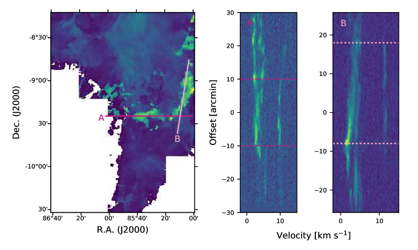
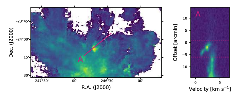
Figures 5 and 7 exhibit several small high- regions. There are high- regions in ISF and L1647 of the Orion A cloud. In the Ophiuchus cloud, there is a small high- region in the northern part of L1688. In each cloud, these regions have that are higher than the typical value of in the other part of the cloud.
Figures C.1 and C.2 show the position-velocity (PV) diagrams for these high- regions in the Orion A cloud. And Figure C.3 presents the PV diagram for the high- region in the Ophiuchus cloud. The PV diagrams demonstrate that there are two cloud components along the lines of sight at the high- regions. Thus, the high- values are caused by multiple gas components with different line of sight velocities. In the ISF region, the interactions between the MC and nearby sources, such as a foreground expending nebula and protostellar outflows, seems to produce these multiple cloud components (Shimajiri et al., 2014; Kong et al., 2018). In the L1647 and L1688 regions, there might be foreground or background cloud components with different line of sight velocities.
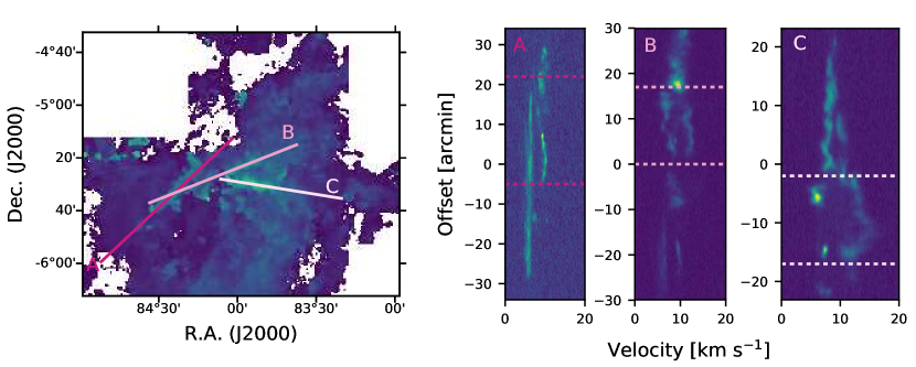
of 13CO (the first panel). The PV diagrams along the solid lines (A, B, and C) are presented on the second, third, and forth panels. The dotted horizontal lines in each PV diagram represents the position of the high- regions on each line. The offset on the y-axis of the PV diagrams indicates a displacement from east to west on the line.
Appendix D Random motion of the L1688 cloud
Because the observed 13CO line can be optically thick toward the dense part of L1688, the map for 13CO (Figure 6) cannot exactly present the global motion of the cloud. Therefore, the optically thinner lines, such as the C18O and CS lines, should be used to trace the global motion. However, the maps of the C18O and CS lines do not present any large-scale motions of the L1688 cloud (Figures B.6 and B.10). Loren (1989b) also suggested that the gas motion in the L1688 cloud is more complex than simple rotation. They measured of the Ophiuchus cores using the 13CO and DCO+ lines and found that the velocity variation for the DCO+ lines is larger than that for the 13CO lines. Therefore, we assume that there is no global motion in L1688.
References
- Aikawa et al. (2001) Aikawa, Y., Ohashi, N., Inutsuka, S.-i., Herbst, E., & Takakuwa, S. 2001, ApJ, 552, 639, doi: 10.1086/320551
- Allen & Davis (2008) Allen, L. E., & Davis, C. J. 2008, Low Mass Star Formation in the Lynds 1641 Molecular Cloud, ed. B. Reipurth, Vol. 4, 621
- André et al. (2010) André, P., Men’shchikov, A., Bontemps, S., et al. 2010, A&A, 518, L102, doi: 10.1051/0004-6361/201014666
- Bally et al. (1987) Bally, J., Langer, W. D., Stark, A. A., & Wilson, R. W. 1987, ApJ, 312, L45, doi: 10.1086/184817
- Bergin & Langer (1997) Bergin, E. A., & Langer, W. D. 1997, ApJ, 486, 316, doi: 10.1086/304510
- Bergin & Tafalla (2007) Bergin, E. A., & Tafalla, M. 2007, ARA&A, 45, 339, doi: 10.1146/annurev.astro.45.071206.100404
- Bianchi (2013) Bianchi, S. 2013, A&A, 552, A89, doi: 10.1051/0004-6361/201220866
- Brunt & Heyer (2013) Brunt, C. M., & Heyer, M. H. 2013, MNRAS, 433, 117
- Brunt et al. (2009) Brunt, C. M., Heyer, M. H., & Mac Low, M. M. 2009, A&A, 504, 883, doi: 10.1051/0004-6361/200911797
- Burkhart et al. (2009) Burkhart, B., Falceta-Gonçalves, D., Kowal, G., & Lazarian, A. 2009, ApJ, 693, 250, doi: 10.1088/0004-637X/693/1/250
- Caselli et al. (1999) Caselli, P., Walmsley, C. M., Tafalla, M., Dore, L., & Myers, P. C. 1999, ApJ, 523, L165, doi: 10.1086/312280
- Chen et al. (2020) Chen, H. H.-H., Offner, S. S. R., Pineda, J. E., et al. 2020, arXiv e-prints, arXiv:2006.07325. https://arxiv.org/abs/2006.07325
- Chen et al. (2019) Chen, H. H.-H., Pineda, J. E., Goodman, A. A., et al. 2019, ApJ, 877, 93, doi: 10.3847/1538-4357/ab1a40
- Dame (2011) Dame, T. M. 2011, arXiv e-prints, arXiv:1101.1499. https://arxiv.org/abs/1101.1499
- Davis et al. (2009) Davis, C. J., Froebrich, D., Stanke, T., et al. 2009, A&A, 496, 153, doi: 10.1051/0004-6361:200811096
- Dobashi et al. (2005) Dobashi, K., Uehara, H., Kandori, R., et al. 2005, PASJ, 57, S1, doi: 10.1093/pasj/57.sp1.S1
- Dunham et al. (2015) Dunham, M. M., Allen, L. E., Evans, II, N. J., et al. 2015, ApJS, 220, 11
- Elmegreen & Scalo (2004) Elmegreen, B. G., & Scalo, J. 2004, ARA&A, 42, 211, doi: 10.1146/annurev.astro.41.011802.094859
- Emerson & Graeve (1988) Emerson, D. T., & Graeve, R. 1988, A&A, 190, 353
- Evans (1999) Evans, Neal J., I. 1999, ARA&A, 37, 311, doi: 10.1146/annurev.astro.37.1.311
- Evans et al. (2020) Evans, Neal J., I., Kim, K.-T., Wu, J., et al. 2020, ApJ, 894, 103, doi: 10.3847/1538-4357/ab8938
- Friesen et al. (2017) Friesen, R. K., Pineda, J. E., co-PIs, et al. 2017, ApJ, 843, 63, doi: 10.3847/1538-4357/aa6d58
- Furlan et al. (2016) Furlan, E., Fischer, W. J., Ali, B., et al. 2016, ApJS, 224, 5
- Gaches et al. (2015) Gaches, B. A. L., Offner, S. S. R., Rosolowsky, E. W., & Bisbas, T. G. 2015, ApJ, 799, 235
- Gill & Henriksen (1990) Gill, A. G., & Henriksen, R. N. 1990, ApJ, 365, L27, doi: 10.1086/185880
- Goodman et al. (1998) Goodman, A. A., Barranco, J. A., Wilner, D. J., & Heyer, M. H. 1998, ApJ, 504, 223, doi: 10.1086/306045
- Goodman et al. (2009) Goodman, A. A., Pineda, J. E., & Schnee, S. L. 2009, ApJ, 692, 91, doi: 10.1088/0004-637X/692/1/91
- Großschedl et al. (2018) Großschedl, J. E., Alves, J., Meingast, S., et al. 2018, A&A, 619, A106, doi: 10.1051/0004-6361/201833901
- Hartmann & Burkert (2007) Hartmann, L., & Burkert, A. 2007, ApJ, 654, 988, doi: 10.1086/509321
- Hasegawa et al. (1984) Hasegawa, T., Kaifu, N., Inatani, J., et al. 1984, ApJ, 283, 117, doi: 10.1086/162280
- Heyer & Brunt (2004) Heyer, M. H., & Brunt, C. M. 2004, ApJ, 615, L45, doi: 10.1086/425978
- Heyer et al. (1992) Heyer, M. H., Morgan, J., Schloerb, F. P., Snell, R. L., & Goldsmith, P. F. 1992, ApJ, 395, L99, doi: 10.1086/186497
- Heyer & Schloerb (1997) Heyer, M. H., & Schloerb, F. P. 1997, ApJ, 475, 173
- Hildebrand (1983) Hildebrand, R. H. 1983, QJRAS, 24, 267
- Ikeda et al. (2007) Ikeda, N., Sunada, K., & Kitamura, Y. 2007, ApJ, 665, 1194, doi: 10.1086/519484
- Jeong et al. (2019) Jeong, I.-G., Kang, H., Jung, J., et al. 2019, Journal of Korean Astronomical Society, 52, 227
- Jiménez-Donaire et al. (2017) Jiménez-Donaire, M. J., Cormier, D., Bigiel, F., et al. 2017, ApJ, 836, L29, doi: 10.3847/2041-8213/836/2/L29
- Johansson et al. (1984) Johansson, L. E. B., Andersson, C., Ellder, J., et al. 1984, A&A, 130, 227
- Johnstone et al. (2004) Johnstone, D., Di Francesco, J., & Kirk, H. 2004, ApJ, 611, L45, doi: 10.1086/423737
- Kauffmann et al. (2017) Kauffmann, J., Goldsmith, P. F., Melnick, G., et al. 2017, A&A, 605, L5, doi: 10.1051/0004-6361/201731123
- Kirk et al. (2017) Kirk, H., Friesen, R. K., Pineda, J. E., et al. 2017, ApJ, 846, 144, doi: 10.3847/1538-4357/aa8631
- Klessen (2000) Klessen, R. S. 2000, ApJ, 535, 869, doi: 10.1086/308854
- Koch et al. (2017) Koch, E. W., Ward, C. G., Offner, S., Loeppky, J. L., & Rosolowsky, E. W. 2017, MNRAS, 471, 1506, doi: 10.1093/mnras/stx1671
- Kong et al. (2018) Kong, S., Arce, H. G., Feddersen, J. R., et al. 2018, ApJS, 236, 25, doi: 10.3847/1538-4365/aabafc
- Kounkel et al. (2018) Kounkel, M., Covey, K., Suárez, G., et al. 2018, AJ, 156, 84, doi: 10.3847/1538-3881/aad1f1
- Kowal et al. (2007) Kowal, G., Lazarian, A., & Beresnyak, A. 2007, ApJ, 658, 423, doi: 10.1086/511515
- Krips et al. (2008) Krips, M., Neri, R., García-Burillo, S., et al. 2008, ApJ, 677, 262, doi: 10.1086/527367
- Kuiper et al. (1980) Kuiper, T. B. H., Kuiper, E. N. R., & Zuckerman, B. 1980, in Interstellar Molecules, ed. B. H. Andrew, Vol. 87, 31
- Kutner et al. (1977) Kutner, M. L., Tucker, K. D., Chin, G., & Thaddeus, P. 1977, ApJ, 215, 521, doi: 10.1086/155384
- Lada & Wilking (1980) Lada, C. J., & Wilking, B. A. 1980, ApJ, 238, 620, doi: 10.1086/158019
- Larson (1981) Larson, R. B. 1981, MNRAS, 194, 809
- Lee et al. (2004) Lee, J.-E., Bergin, E. A., & Evans, Neal J., I. 2004, ApJ, 617, 360, doi: 10.1086/425153
- Lee et al. (2003) Lee, J.-E., Evans, Neal J., I., Shirley, Y. L., & Tatematsu, K. 2003, ApJ, 583, 789, doi: 10.1086/345428
- Loren (1989a) Loren, R. B. 1989a, ApJ, 338, 902, doi: 10.1086/167244
- Loren (1989b) —. 1989b, ApJ, 338, 925, doi: 10.1086/167245
- Loren et al. (1990) Loren, R. B., Wootten, A., & Wilking, B. A. 1990, ApJ, 365, 269, doi: 10.1086/169480
- Lynds (1962) Lynds, B. T. 1962, ApJS, 7, 1, doi: 10.1086/190072
- Mac Low & Klessen (2004) Mac Low, M.-M., & Klessen, R. S. 2004, Reviews of Modern Physics, 76, 125, doi: 10.1103/RevModPhys.76.125
- Maddalena et al. (1986) Maddalena, R. J., Morris, M., Moscowitz, J., & Thaddeus, P. 1986, ApJ, 303, 375, doi: 10.1086/164083
- Mairs et al. (2016) Mairs, S., Johnstone, D., Kirk, H., et al. 2016, MNRAS, 461, 4022, doi: 10.1093/mnras/stw1550
- Megeath et al. (2012) Megeath, S. T., Gutermuth, R., Muzerolle, J., et al. 2012, AJ, 144, 192
- Meingast et al. (2016) Meingast, S., Alves, J., Mardones, D., et al. 2016, A&A, 587, A153, doi: 10.1051/0004-6361/201527160
- Méndez-Hernández et al. (2020) Méndez-Hernández, H., Ibar, E., Knudsen, K. K., et al. 2020, MNRAS, 497, 2771, doi: 10.1093/mnras/staa1964
- Monsch et al. (2018) Monsch, K., Pineda, J. E., Liu, H. B., et al. 2018, ApJ, 861, 77, doi: 10.3847/1538-4357/aac8da
- Motte et al. (1998) Motte, F., Andre, P., & Neri, R. 1998, A&A, 336, 150
- Nagahama et al. (1998) Nagahama, T., Mizuno, A., Ogawa, H., & Fukui, Y. 1998, AJ, 116, 336, doi: 10.1086/300392
- Nakamura et al. (2012) Nakamura, F., Miura, T., Kitamura, Y., et al. 2012, ApJ, 746, 25, doi: 10.1088/0004-637X/746/1/25
- Nakamura et al. (2019) Nakamura, F., Ishii, S., Dobashi, K., et al. 2019, PASJ, 71, S3, doi: 10.1093/pasj/psz057
- Olofsson et al. (1982) Olofsson, H., Ellder, J., Hjalmarson, A., & Rydbeck, G. 1982, A&A, 113, L18
- Ortiz-León et al. (2017) Ortiz-León, G. N., Loinard, L., Kounkel, M. A., et al. 2017, ApJ, 834, 141, doi: 10.3847/1538-4357/834/2/141
- Ossenkopf & Mac Low (2002) Ossenkopf, V., & Mac Low, M. M. 2002, A&A, 390, 307, doi: 10.1051/0004-6361:20020629
- Padoan et al. (1999) Padoan, P., Bally, J., Billawala, Y., Juvela, M., & Nordlund, Å. 1999, ApJ, 525, 318, doi: 10.1086/307864
- Padoan et al. (2001) Padoan, P., Juvela, M., Goodman, A. A., & Nordlund, Å. 2001, ApJ, 553, 227, doi: 10.1086/320636
- Padoan et al. (2006) Padoan, P., Juvela, M., Kritsuk, A., & Norman, M. L. 2006, ApJ, 653, L125, doi: 10.1086/510620
- Padoan et al. (2009) —. 2009, ApJ, 707, L153, doi: 10.1088/0004-637X/707/2/L153
- Pan et al. (2017) Pan, Z., Li, D., Chang, Q., et al. 2017, ApJ, 836, 194, doi: 10.3847/1538-4357/aa5c33
- Pattle et al. (2015) Pattle, K., Ward-Thompson, D., Kirk, J. M., et al. 2015, MNRAS, 450, 1094, doi: 10.1093/mnras/stv376
- Pety et al. (2017) Pety, J., Guzmán, V. V., Orkisz, J. H., et al. 2017, A&A, 599, A98, doi: 10.1051/0004-6361/201629862
- Punanova et al. (2016) Punanova, A., Caselli, P., Pon, A., Belloche, A., & André, P. 2016, A&A, 587, A118, doi: 10.1051/0004-6361/201527592
- Ridge et al. (2006) Ridge, N. A., Di Francesco, J., Kirk, H., et al. 2006, AJ, 131, 2921, doi: 10.1086/503704
- Ripple et al. (2013) Ripple, F., Heyer, M. H., Gutermuth, R., Snell, R. L., & Brunt, C. M. 2013, MNRAS, 431, 1296, doi: 10.1093/mnras/stt247
- Roh & Jung (1999) Roh, D.-G., & Jung, J. H. 1999, Publication of Korean Astronomical Society, 14, 123
- Roy et al. (2013) Roy, A., Martin, P. G., Polychroni, D., et al. 2013, ApJ, 763, 55, doi: 10.1088/0004-637X/763/1/55
- Rydbeck et al. (1981) Rydbeck, O. E. H., Hjalmarson, A., Rydbeck, G., et al. 1981, ApJ, 243, L41, doi: 10.1086/183439
- Shimajiri et al. (2011) Shimajiri, Y., Kawabe, R., Takakuwa, S., et al. 2011, PASJ, 63, 105, doi: 10.1093/pasj/63.1.105
- Shimajiri et al. (2014) Shimajiri, Y., Kitamura, Y., Saito, M., et al. 2014, A&A, 564, A68
- Shimajiri et al. (2017) Shimajiri, Y., André, P., Braine, J., et al. 2017, A&A, 604, A74, doi: 10.1051/0004-6361/201730633
- Solomon et al. (1987) Solomon, P. M., Rivolo, A. R., Barrett, J., & Yahil, A. 1987, ApJ, 319, 730, doi: 10.1086/165493
- Storm et al. (2014) Storm, S., Mundy, L. G., Fernández-López, M., et al. 2014, ApJ, 794, 165
- Storm et al. (2016) Storm, S., Mundy, L. G., Lee, K. I., et al. 2016, ApJ, 830, 127, doi: 10.3847/0004-637X/830/2/127
- Tatematsu et al. (2008) Tatematsu, K., Kandori, R., Umemoto, T., & Sekimoto, Y. 2008, PASJ, 60, 407, doi: 10.1093/pasj/60.3.407
- Tatematsu et al. (1993) Tatematsu, K., Umemoto, T., Kameya, O., et al. 1993, ApJ, 404, 643, doi: 10.1086/172318
- Ungerechts et al. (1997) Ungerechts, H., Bergin, E. A., Goldsmith, P. F., et al. 1997, ApJ, 482, 245, doi: 10.1086/304110
- van Dishoeck et al. (1995) van Dishoeck, E. F., Blake, G. A., Jansen, D. J., & Groesbeck, T. D. 1995, ApJ, 447, 760, doi: 10.1086/175915
- Wannier & Phillips (1977) Wannier, P. G., & Phillips, T. G. 1977, ApJ, 215, 796, doi: 10.1086/155415
- Wilking et al. (2008) Wilking, B. A., Gagné, M., & Allen, L. E. 2008, Star Formation in the Ophiuchi Molecular Cloud, ed. B. Reipurth, Vol. 5, 351
- Wilson & Rood (1994) Wilson, T. L., & Rood, R. 1994, ARA&A, 32, 191, doi: 10.1146/annurev.aa.32.090194.001203
- Zhang & Wang (2009) Zhang, M., & Wang, H. 2009, AJ, 138, 1830, doi: 10.1088/0004-6256/138/6/1830