A Regression-based Approach to Robust Estimation and Inference for Genetic Covariance

Abstract

Genome-wide association studies (GWAS) have identified thousands of genetic variants associated with complex traits, and some variants are shown to be associated with multiple complex traits. Genetic covariance between two traits is defined as the underlying covariance of genetic effects and can be used to measure the shared genetic architecture. The data used to estimate such a genetic covariance can be from the same group or different groups of individuals, and the traits can be of different types or collected based on different study designs. This paper proposes a unified regression-based approach to robust estimation and inference for genetic covariance of general traits that may be associated with genetic variants nonlinearly. The asymptotic properties of the proposed estimator are provided and are shown to be robust under certain model mis-specification. Our method under linear working models provides a robust inference for the narrow-sense genetic covariance, even when both linear models are mis-specified. Numerical experiments are performed to support the theoretical results. Our method is applied to an outbred mice GWAS data set to study the overlapping genetic effects between the behavioral and physiological phenotypes. The real data results reveal interesting genetic covariance among different mice developmental traits.

Keywords: genetic relatedness, model mis-specification, narrow-sense genetic covariance, regularization, bias correction

1 Introduction

Genome-wide association studies (GWAS) have identified thousands of variants related to complex traits. Some complex traits are shown to have a shared genetic etiology, including various autoimmune diseases (Li et al., 2015) and psychiatric disorders (Cross-Disorder Group of the Psychiatric Genomics Consortium, 2019). Studying the shared genetic architecture and investigating the relationship between the genetics of different traits can provide insights into the underlying biological mechanism. There has been a great interest in quantifying the overlapping genetic effects between pairs of traits based on GWAS data. With individual-level genotype data, genetic effects on the traits can be modeled by some functions of the observed genetic variants such as linear functions, and the single nucleotide polymorphism (SNP)-based estimate of genetic covariance can be derived (Lee et al., 2012; Bulik-Sullivan et al., 2015) based on the assumed models.

Although estimating the shared genetic effects has received much attention recently, several issues remain to be addressed. First, most existing literature focuses on traits that are generated from linear models. For binary traits, such as the occurrences of diseases, linear models are not suitable. However, there are few approaches with theoretical guarantees for dealing with nonlinear trait models. Second, the true underlying models for the traits are unknown in practice and need to be specified. When the models are mis-specified, the estimated genetic effects and the corresponding genetic covariance can be biased. For estimating the shared genetic effects between two traits, model mis-specification is more likely to happen. Thus, it is important to develop robust methods for estimating the genetic covariance. Third, the genetic data sets can be collected based on different designs, further complicating the analysis of genetic covariance. For example, two traits and the corresponding genotypes may be collected on the same samples or independent samples. In a more challenging scenario, one trait may be collected from a cohort study, while the other may be from a case-control study. As far as we know, existing methods cannot be directly applied to such data or do not have any statistical guarantee.

Motivated by the challenges mentioned above, we study estimation and inference for genetic covariance based on the individual-level GWAS data. We consider generic population models for the trait that is possibly associated with the genotypes nonlinearly. Specifically, we consider the following models for the two traits,

$$y_{i}=f^{*}(x_{i})+\varepsilon^{*}_{i},\quad z_{i}=g^{*}(x_{i})+v^{*}_{i},$$ (1)

where $y_{i}$ and $z_{i}$ are two trait values, including continuous complex trait measures, disease outcomes, or gene expressions, and $x_{i}^{\intercal}=(x_{i1},\cdots,x_{ip})^{\intercal}\in\mathcal{R}^{p}$ denotes the $i$-th observation of $p$ genetic variants, each coded as 0, 1 and 2. In typical GWAS, $p$ can be larger and much larger than the sample sizes. The functions $f^{*}(\cdot)$ and $g^{*}(\cdot)$ denote the true conditional mean functions of $y_{i}$ and $z_{i}$, respectively, such that $\mathrm{E}[\varepsilon^{*}_{i}\mid x_{i}]=\mathrm{E}[v^{*}_{i}\mid x_{i}]=0$. In genetic terms, $f^{*}(x_{i})$ is the genetic effect of $y_{i}$, representing the total effects of all the genetic variants considered. The error terms $\varepsilon^{*}_{i}$ and $v^{*}_{i}$ can be dependent due to possible confounding effects. The functions $f^{*}(\cdot)$ and $g^{*}(\cdot)$ can be known or unknown. We emphasize that Model (1) includes a general class of trait models, which can be parametric or non-parametric.

First considered in Searle (1961), the genetic covariance of traits $y_{i}$ and $z_{i}$ is defined as the covariance of their conditional mean functions $f^{*}(x_{i})$ and $g^{*}(x_{i})$ ,

$$I^{*}=\mathrm{Cov}(\mathrm{E}[y_{i}|x_{i}],\mathrm{E}[z_{i}|x_{i}])=\mathrm{Cov}(f^{*}(x_{i}),g^{*}(x_{i})).$$ (2)

Invoking the law of total variance formula, parameter $I^{*}$ represents the covariance of two traits explained by genetic variants. When the traits are binary, this genetic covariance is defined at the observed scale instead of the liability scale as commonly used in probit-mixed effect models. A closely related concept is heritability. The heritability of trait $y_{i}$ is defined as $\mathrm{Var}(f^{*}(x_{i}))/\mathrm{Var}(y_{i})$, which is the proportion of phenotypic variance explained by genetic variants.

While $I^{*}$ captures the covariance due to total genetic effects, sometimes the contribution of additive genetic effects can be of interest, especially for continuous complex traits. Analogous to the narrow-sense heritability (Tenesa and Haley, 2013), the narrow-sense genetic covariance measures the additive genetic covariance by fitting linear models to the traits. Specifically, narrow-sense genetic covariance is defined as the bilinear functional $\beta^{\intercal}\Sigma\gamma$, where $\beta$ and $\gamma$ are the regression coefficients in the linear models representing the additive effects, $f^{*}(x_{i})=\beta_{0}+x_{i}\beta$ and $g^{*}(x_{i})=\gamma_{0}+x_{i}\gamma$, and $\Sigma$ is the covariance of $x_{i}$. We mention that even if $f^{*}(\cdot)$ or $g^{*}(\cdot)$ are nonlinear functions, one can still define $\beta$ and $\gamma$ through working linear models. That is, even if the linear models are wrongly specified, the definition of narrow-sense genetic covariance is still valid but $I^{*}\neq\beta^{\intercal}\Sigma\gamma$ in general. Formal definitions of $\beta$ and $\gamma$ are given in (3). As far as we know, the estimation and inference for $\beta^{\intercal}\Sigma\gamma$ have not been studied when the linear models are mis-specified. It is unknown whether existing methods are valid for the inference on $\beta^{\intercal}\Sigma\gamma$ under model mis-specification.

1.1 Related literature

Many methods have been proposed for estimating heritability and genetic covariance in genetics literature. Among them, the linear mixed-effects model is one of the most popular choices and is adopted in the GCTA-GREML method (Lee et al., 2013) and linkage disequilibrium score regression (LDSC) method (Bulik-Sullivan et al., 2015). In a linear mixed-effects model, the effects of genetic variants are assumed to be i.i.d. normally distributed and the genetic covariance equals the covariance between the random effects with the genotype data standardized to have a unit variance. A closely related model is the latent liability model (Lee et al., 2013) for binary traits, which can be viewed as a random-effects probit model. Despite their popularity, the assumptions of liability model or linear random-effects models have been questioned and their estimates are not robust to the distributional assumptions on the effects (Speed et al., 2017; Wang and Li, 2022). Some partition-based methods have been proposed to improve the heritability estimation (Yang et al., 2015; Gazal et al., 2017), where more complicated random-effects models are used to make the estimation accurate (Gazal et al., 2019; Evans et al., 2018).

The estimation and inference for heritability and genetic relatedness in fixed-effects linear trait models have been studied in statistics literature. Assuming correctly specified high-dimensional linear models, Cai and Guo (2020) studies estimation and inference for heritability based on the penalized regressions. Verzelen and Gassiat (2018) proposes an adaptive procedure to estimate heritability by combining the sparsity-based method and the method of moments in linear models. Guo et al. (2019) studies the estimation of genetic relatedness $\beta^{\intercal}\gamma$ between two continuous traits in correctly-specified high-dimensional linear models, which is closely related to the genetic covariance. They assume that the noises in the two traits models are independent, but do not provide methods for inference.

1.2 Our contributions

As we reviewed above, most of existing methods for estimating the genetic covariance are developed for continuous traits assuming correctly specified linear models and the independence of the errors of the two traits. A robust inference procedure is needed when any of the model assumptions are violated. Our paper aims to fill this gap. We propose a regression-based approach to the estimation and inference of genetic covariance $I^{*}$ defined as equation (2) for the traits that can be nonlinearly associated with high-dimensional genetic variants. Based on sparse high-dimensional generalized linear models (GLMs) as working models, we propose an estimator and construct the confidence interval for genetic covariance. Our method makes use of all the available observations, allowing samples for the two traits to overlap. Our approach can also be used to estimate and make inferences for the narrow-sense genetic covariance $\beta^{\intercal}\Sigma\gamma$ when linear working models are assumed.

We show the robustness of the proposed estimator of genetic covariance. Firstly, when both working models are correctly specified GLMs, the proposed method provides an asymptotically normal estimator for $I^{*}$ under proper conditions. Secondly, when the models are possibly mis-specified, the proposed estimator is still consistent as long as one conditional mean model is correctly specified. If one linear working model is used and is correctly specified, then the asymptotic normality of our estimator of $I^{*}$ still holds under certain sparsity conditions.

The rest of the paper is organized as follows. Section 2 introduces a unified method of estimation and inference for genetic covariance and narrow-sense genetic covariance. Section 3 establishes the theoretical properties of our estimator for the genetic covariance under correct or mis-specified models, including the method for estimating the narrow-sense generic covariance. In Section 4, the performance of the estimator is evaluated in different settings using numerical experiments. In Section 5, the proposed method is applied to an outbred mice data set to study the genetic covariance between the behavioral and physiological traits. A discussion is provided in Section 6. The proofs of main theorems and the extended simulation studies are given in the Supplementary Materials.

Notations

Given a symmetric matrix $A$, we use $\left\lVert A\right\rVert_{2}$ to denote the $\ell_{2}$-operator norm and $\lambda_{\max}({A})$ and $\lambda_{\min}({A})$ respectively to denote the largest and the smallest eigenvalue of $A$. For a design matrix $X\in\mathcal{R}^{n\times p},$ let $x_{i}$ denote the $i$-th row of $X$, and $x_{ij}$ denote the $j$-th element of the row vector $x_{i}.$ For an index set $\mathcal{I}$, we denote its cardinality as $|\mathcal{I}|$. For a vector $u$, its support is represented by ${\rm supp}(u).$ For two positive sequences $a_{n}$ and $b_{n}$, $a_{n}\lesssim b_{n}$ means $a_{n}\leq Cb_{n}$ for sufficiently large $n$, $a_{n}\gtrsim b_{n}$ if $b_{n}\lesssim a_{n}$ and $a_{n}\asymp b_{n}$ if $a_{n}\lesssim b_{n}$ and $b_{n}\lesssim a_{n}$. We write $b_{n}\ll a_{n}$ if $\lim\sup b_{n}/a_{n}\to 0.$ $c$ and $C$ are used to denote generic positive constants that may vary from place to place.

2 Estimation of genetic covariance and construction of confidence interval

2.1 Fitting the working models

To estimate the genetic covariance, we consider fitting potentially mis-specified GLMs to the two traits (Nelder and Wedderburn, 1972). The fitted models are treated as working models. In GLMs with canonical link functions, the regression coefficients $\beta$ and $\gamma$ are defined as the minimizer of the population negative log-likelihood functions, i.e.,

$$(\beta_{0},\beta)=\operatorname*{arg\,min}_{\beta_{0}\in\mathcal{R},\,\beta\in\mathcal{R}^{p}}\mathrm{E}\left[F(\beta_{0}+x_{i}\beta)-y_{i}(\beta_{0}+x_{i}\beta)\right]$$

$$(\gamma_{0},\gamma)=\operatorname*{arg\,min}_{\gamma_{0}\in\mathcal{R},\,\gamma\in\mathcal{R}^{p}}\mathrm{E}[G(\gamma_{0}+x_{i}\gamma)-z_{i}(\gamma_{0}+x_{i}\gamma)].$$ (3)

Functions $F(t)$ and $G(t)$ have known parametric forms, for example, $F(t)=t^{2}/2$ gives a linear model and $F(t)=\log(1+\exp(t))$ gives a logistic model. For differentiable $F(t)$ and $G(t)$, $f(t)=F^{\prime}(t)$ and $g(t)=G^{\prime}(t)$ are the working models for modeling the conditional mean of the traits. We can re-express the working GLM models (3) as

$$y_{i}=f(\beta_{0}+x_{i}\beta)+\varepsilon_{i}~{}~{}\text{and}~{}~{}z_{i}=g(\gamma_{0}+x_{i}\gamma)+v_{i},$$ (4)

where $\mathrm{E}[x_{i}\varepsilon_{i}]=0$ and $\mathrm{E}[x_{i}v_{i}]=0$ by taking derivatives in (3). We mention that including the intercepts $\beta_{0}$ and $\gamma_{0}$ is crucial when the models are possibly mis-specified as it guarantees $\mathrm{E}[\varepsilon_{i}]=\mathrm{E}[v_{i}]=0$. For typical GWAS data sets, the number of genetic variants $p$ is very large, we often assume that the coefficients $(\beta,\gamma)$ in these working models are sparse. With linear working models $f(\beta_{0}+x_{i}\beta)=\beta_{0}+x_{i}\beta$ and $g(\gamma_{0}+x_{i}\gamma)=\gamma_{0}+x_{i}\gamma$, the narrow-sense genetic covariance is defined as the bilinear functional $\mathrm{Cov}(x_{i}\beta,x_{i}\gamma)=\beta^{\intercal}\Sigma\gamma$. Again, it is defined with respect to the working models instead of the true models.

To make inference of $I^{*}$ defined in (2), our proposal is based on sample splitting. We use index sets $\mathcal{I}^{0}_{y}$ and $\mathcal{I}^{0}_{z}$ to represent the collected individuals for traits $y$ and $z$, respectively. We randomly split samples so that samples for estimating the coefficients in model (4) and samples for constructing the estimator of covariance are independent. Without loss of generality, we assume that $|\mathcal{I}^{0}_{y}|=2n_{y}$ and $|\mathcal{I}^{0}_{z}|=2n_{z}$. We split $\mathcal{I}^{0}_{y}$ into two disjoint subsets $\tilde{\mathcal{I}}_{y}$ and $\mathcal{I}_{y}$ with $|\tilde{\mathcal{I}}_{y}|=|\mathcal{I}_{y}|=n_{y}$ and split $\mathcal{I}^{0}_{z}$ into two disjoint subsets $\tilde{\mathcal{I}}_{z}$ and $\mathcal{I}_{z}$ with $|\tilde{\mathcal{I}}_{z}|=|\mathcal{I}_{z}|=n_{z}$.

Based on the samples in $\tilde{\mathcal{I}}_{y}$ and $\tilde{\mathcal{I}}_{z}$, the coefficients ${\beta}$ and ${\gamma}$ are estimated by minimizing the following penalized negative log-likelihood functions

$$(\hat{\beta}_{0},\hat{\beta}) =\operatorname*{arg\,min}_{\beta_{0}\in\mathcal{R},\,\beta\in\mathcal{R}^{p}}|\tilde{\mathcal{I}}_{y}|^{-1}\sum_{i\in\tilde{\mathcal{I}}_{y}}\left\{(F(\beta_{0}+x_{i}\beta)-y_{i}(\beta_{0}+x_{i}\beta)\right\}+\lambda_{\beta}(|\beta_{0}|+\left\lVert\beta\right\rVert_{1})\,,$$ (5)

$$(\hat{\gamma}_{0},\hat{\gamma}) =\operatorname*{arg\,min}_{\gamma_{0}\in\mathcal{R},\,\gamma\in\mathcal{R}^{p}}|\tilde{\mathcal{I}}_{z}|^{-1}\sum_{i\in\tilde{\mathcal{I}}_{z}}\left\{G(\gamma_{0}+x_{i}\gamma)-z_{i}(\gamma_{0}+x_{i}\gamma)\right\}+\lambda_{\gamma}(|\gamma_{0}|+\|\gamma\|_{1}),$$ (6)

where $\lambda_{\beta}>0$ and $\lambda_{\gamma}>0$ are tuning parameters.

2.2 Estimating the genetic covariance

In the second step of our approach, we construct the estimator for genetic covariance $I^{*}$ using samples in $\mathcal{I}_{y}$ and $\mathcal{I}_{z}$. First, we plug in the coefficient estimates $\hat{\beta}$ and $\hat{\gamma}$, and obtain the residuals $\hat{\varepsilon}_{i}=y_{i}-f(\hat{\beta}_{0}+x_{i}\hat{\beta})$ for $i\in\mathcal{I}_{y}$ and $\hat{v}_{i}=z_{i}-g(\hat{\gamma}_{0}+x_{i}\hat{\gamma})$ for $i\in\mathcal{I}_{z}$. To make use of all observed genotypes, we impute the two traits using the predicted values $f(\hat{\beta}_{0}+x_{i}\hat{\beta})$ and $g(\hat{\gamma}_{0}+x_{i}\hat{\gamma})$ from the working GLMs for all $i\in\mathcal{I}_{y}\cup\mathcal{I}_{z}.$ Here $\mathcal{I}_{y}\cup\mathcal{I}_{z}$ is the index set of all unique samples and $N=|\mathcal{I}_{y}\cup\mathcal{I}_{z}|$ denotes its cardinality. The predicted traits are used to estimate $\mathrm{E}[f(\beta_{0}+x_{i}\beta)g(\gamma_{0}+x_{i}\gamma)]$, which may differ from the predicted values obtained from the true model.

In model (1), $I^{*}$ can be expressed as (dropping $x_{i}$ for simplicity) $I^{*}=\mathrm{Cov}(f_{i}^{*},g_{i}^{*})=\mathrm{E}[f_{i}^{*}g_{i}^{*}]-\mathrm{E}[f_{i}^{*}]\mathrm{E}[g_{i}^{*}].$ We estimate $\mathrm{E}[f_{i}^{*}g_{i}^{*}]$ and $\mathrm{E}[f_{i}^{*}]\mathrm{E}[g_{i}^{*}]$ separately. We mention that $\mathrm{E}[f_{i}^{*}]$ and $\mathrm{E}[g_{i}^{*}]$ are zero in linear models but are possibly nonzero for nonlinear functions $f^{*}(\cdot)$ and $g^{*}(\cdot)$, and hence require separate estimates. To motivate our estimator of $\mathrm{E}[f_{i}^{*}g_{i}^{*}],$ let
$\widehat{E}^{\text{plug}}=N^{-1}\sum_{i\in\mathcal{I}_{y}\cup\mathcal{I}_{z}}{f(\hat{\beta}_{0}+x_{i}\hat{\beta})g(\hat{\gamma}_{0}+x_{i}\hat{\gamma})}$ denote the simple plug-in estimator based on the specified working models. The plug-in estimator $\widehat{E}^{\text{plug}}$ is sensitive to the model specification. Specifically, let $f_{i}$ and $g_{i}$ denote $f(\beta_{0}+x_{i}\beta)$ and $g(\gamma_{0}+x_{i}\gamma)$, respectively. The difference between $\mathrm{E}[f_{i}^{*}g_{i}^{*}]$ and $\mathrm{E}[f_{i}g_{i}]$ is

$$\mathrm{E}[f_{i}^{*}g_{i}^{*}]-\mathrm{E}[f_{i}g_{i}]=\mathrm{E}[g_{i}(f_{i}^{*}-f_{i})]+\mathrm{E}[f_{i}(g_{i}^{*}-g_{i})]+\mathrm{E}[(f_{i}^{*}-f_{i})(g_{i}^{*}-g_{i})].$$ (7)

When $f(\cdot)$ or $g(\cdot)$ is mis-specified, we see from (7) that $\mathrm{E}[f_{i}g_{i}]$ is a biased approximation of the parameter of interest $\mathrm{E}[f_{i}^{*}g_{i}^{*}]$. To reduce the bias on the right-hand side of (7), we use the empirical residuals $\hat{\varepsilon}_{i}$ to estimate $f^{*}_{i}-f_{i}$, and $\hat{v}_{i}$ to estimate $g^{*}_{i}-g_{i}$.

We propose the following estimator of $I^{*}$,

$$\widehat{I}=\sum_{i\in\mathcal{I}_{y}\cup\mathcal{I}_{z}}\frac{f(\hat{\beta}_{0}+x_{i}\hat{\beta})g(\hat{\gamma}_{0}+x_{i}\hat{\gamma})}{N}+\sum_{i\in\mathcal{I}_{z}}\frac{\hat{v}_{i}f(\hat{\beta}_{0}+x_{i}\hat{\beta})}{n_{z}}+\sum_{i\in\mathcal{I}_{y}}\frac{\hat{\varepsilon}_{i}g(\hat{\gamma}_{0}+x_{i}\hat{\gamma})}{n_{y}}-\hat{\mu}_{f}\hat{\mu}_{g},$$ (8)

where $\hat{\mu}_{f}=N^{-1}\sum_{i\in\mathcal{I}_{y}\cup\mathcal{I}_{z}}{f(\hat{\beta}_{0}+x_{i}\hat{\beta})}+n^{-1}_{y}\sum_{i\in\mathcal{I}_{y}}{\hat{\varepsilon}_{i}}$ and $\hat{\mu}_{g}=N^{-1}\sum_{i\in\mathcal{I}_{y}\cup\mathcal{I}_{z}}{g(\hat{\gamma}_{0}+x_{i}\hat{\gamma})}+n^{-1}_{z}\sum_{i\in\mathcal{I}_{z}}{\hat{v}_{i}}$ are estimates of $\mathrm{E}[f_{i}^{*}]$ and $\mathrm{E}[g_{i}^{*}]$, respectively. The sum of the first three terms in $\widehat{I}$ is the estimate of $\mathrm{E}[f_{i}^{*}g_{i}^{*}]$. The imputation step makes the first term in $\widehat{I}$ an average of $N$ random variables. In general, $N=n_{y}+n_{z}-|\mathcal{I}_{y}\cap\mathcal{I}_{z}|$. When two traits are collected from the same group of individuals, $\mathcal{I}_{y}=\mathcal{I}_{z}$ and $N=n_{y}=n_{z}$. When two traits are collected from different groups of individuals, $\mathcal{I}_{y}\cap\mathcal{I}_{z}=\emptyset$ and $N=n_{y}+n_{z}$. With two traits collected separately, the imputation step is essential because there are no matched pairs, $(f_{i},g_{i})$ and $(f_{i},v_{i})$ or $(g_{i},\varepsilon_{i}),$ available from the data.

2.3 Constructing confidence interval for genetic covariance

To construct the confidence interval for $I^{*}$, we are left to devise a variance estimator for $\widehat{I}$. However, after considering potential model mis-specification, the analytical expression of variance could be tedious to calculate, if not impossible. We consider an estimate based on the empirical values rather than the limiting distribution. Denote the centered estimated values as $f^{c}(x_{i}\hat{\beta})=f(\hat{\beta}_{0}+x_{i}\hat{\beta})-\hat{\mu}_{f}$ and $g^{c}(x_{i}\hat{\gamma})=g(\hat{\gamma}_{0}+x_{i}\hat{\gamma})-\hat{\mu}_{g}.$ Let $\mathbbm{1}(\cdot)$ represent the indicator function and we define the empirical value $\widehat{\Delta}_{i}$ as

$$\widehat{\Delta}_{i}=\frac{f^{c}({x_{i}}\hat{\beta})g^{c}(x_{i}\hat{\gamma})}{N}+\frac{\hat{\varepsilon}_{i}g^{c}(x_{i}\hat{\gamma})}{n_{y}}\mathbbm{1}(i\in\mathcal{I}_{y})+\frac{\hat{v}_{i}f^{c}({x_{i}}\hat{\beta})}{n_{z}}\mathbbm{1}(i\in\mathcal{I}_{z}).$$ (9)

We notice that $\widehat{I}$ can be rewritten as the sum of $\widehat{\Delta}_{i}$, i.e., $\widehat{I}=\sum_{i\in\mathcal{I}_{y}\cup\mathcal{I}_{z}}\widehat{\Delta}_{i}.$ Hence, a natural variance estimator for $\widehat{I}$ is $\widehat{\sigma}^{2}=\sum_{i\in\mathcal{I}_{y}\cup\mathcal{I}_{z}}(\widehat{\Delta}_{i}-N^{-1}{\widehat{I}})^{2}$. Our proposed $(1-\alpha)\times 100\%$ two-sided confidence interval for $I^{*}$ is defined as

$$CI(\alpha)=[\widehat{I}-z_{1-\alpha/2}\widehat{\sigma},\widehat{I}+z_{1-\alpha/2}\widehat{\sigma}],$$ (10)

where $z_{1-\alpha/2}$ is the upper $\alpha/2$ quantile of standard normal distribution.

We summarize our proposed procedure in Algorithm 1. The method can be extended for estimating the genetic covariance in case-control studies via bias correction of the intercepts and by using weighting to correct the over-sampling of cases (Section A of the Supplemental Materials). The proposed method can also be used to estimate the heritability by setting $z_{i}=y_{i}$. With data from the same group of individuals, the proposed estimator for heritability generalizes Cai and Guo (2020) to nonlinear trait models.

Input : $(y_{i},x_{i})$ for $i\in\mathcal{I}^{0}_{y}$, $(z_{i},x_{i})$ for $i\in\mathcal{I}^{0}_{z}$, $\lambda_{\beta}$, $\lambda_{\gamma}$, confidence level $\alpha$.

Output : $\widehat{I}$ and $CI(\alpha)$.

1. Split $\mathcal{I}^{0}_{y}$ into $\tilde{\mathcal{I}}_{y}$ and $\mathcal{I}_{y}$. Split $\mathcal{I}^{0}_{z}$ into $\tilde{\mathcal{I}}_{z}$ and $\mathcal{I}_{z}$.

2. Estimate the $\hat{\beta}$ and $\hat{\gamma}$ as in (5) based on samples in $\tilde{\mathcal{I}}_{y}$ and $\tilde{\mathcal{I}}_{z}$.

3. Calculate $\hat{\varepsilon}_{i}=y_{i}-f(\hat{\beta}_{0}+x_{i}\hat{\beta})$ for $i\in\mathcal{I}_{y}$ , $\hat{v}_{i}=z_{i}-g(\hat{\gamma}_{0}+x_{i}\hat{\gamma})$ for $i\in\mathcal{I}_{z}$. Estimate the genetic covariance $\widehat{I}$ as in (8).

4. Calculate $\hat{\Delta}_{i}$ via (9) and empirical variance estimator $\widehat{\sigma}^{2}$. Construct $CI(\alpha)$ as in (10).

Algorithm 1 Estimation and inference for genetic covariance

2.4 Inference for the narrow-sense genetic covariance under linear working models

If the narrow-sense genetic covariance $\beta^{\intercal}\Sigma\gamma$ is used, its estimation and inference can be achieved by choosing the working models $f(\hat{\beta}_{0}+x_{i}\hat{\beta})=\hat{\beta}_{0}+x_{i}\hat{\beta}$ and $g(\hat{\gamma}_{0}+x_{i}\hat{\gamma})=\hat{\gamma}_{0}+x_{i}\hat{\gamma}$. In this case, $\widehat{I}$ can be viewed as a de-biased estimator of $\beta^{\intercal}\Sigma\gamma$. Since the linear working models may be mis-specified, the proposed empirical variance estimator $\widehat{\sigma}^{2}$ is crucial. This is different from the setting of correctly specified linear models, where inference methods can be derived based on the limiting distribution (Janson et al., 2017; Cai and Guo, 2020).

3 Asymptotic normality and robustness

Let $s_{\beta}=|{\rm supp}(\beta)|+\mathbbm{1}(\beta_{0}\neq 0)$ and $s_{\gamma}=|{\rm supp}({\gamma})|+\mathbbm{1}(\gamma_{0}\neq 0)$ denote the sparsity of coefficients defined in (4). We state following assumptions for theoretical analysis.

Assumption 1.

The observed variants $x_{i}$ are $i.i.d.$ samples with mean zero, $\mathrm{E}(x_{i}^{\intercal}x_{i})=\Sigma$, and bounded sub-Gaussian norm. The eigenvalues of $\Sigma$ satisfy $C\leq\lambda_{\min}(\Sigma)\leq\lambda_{\max}(\Sigma)\leq C^{-1}<\infty.$

Assumption 2.

The traits $y_{i}$ and $z_{i}$ are sub-Gaussian random variables with the bounded sub-Gaussian norm. The error terms $\varepsilon^{*}_{i}$ and $v^{*}_{i}$ are sub-Gaussian random variables with mean zero and the bounded sub-Gaussian norm. Besides, $\min\{\mathrm{Var}(\varepsilon^{*}_{i}),\mathrm{Var}(v^{*}_{i})\}\geq c>0$.

Assumption 3.

The functions $F(t)$ and $G(t)$ are twice differentiable with $f(t)=F^{\prime}(t)$ and $g(t)=G^{\prime}(t)$. The derivatives of $f(t)$ and $g(t)$ are uniformly bounded, i.e., $|f^{\prime}(\cdot)|\leq C<\infty$ and $|g^{\prime}(\cdot)|\leq C<\infty.$ Moreover, $f^{\prime}(t)$ and $g^{\prime}(t)$ satisfy the Lipschitz condition for a positive constant $L>0,$

$$\max_{i\in\mathcal{I}^{0}_{y}\cup\mathcal{I}^{0}_{z}}|f^{\prime}(\beta_{0}+x_{i}\beta)-f^{\prime}(\beta_{0}+x_{i}\beta+\theta)|\leq L|\theta|,~{}~{}\max_{i\in\mathcal{I}^{0}_{y}\cup\mathcal{I}^{0}_{z}}|g^{\prime}(\gamma_{0}+x_{i}\gamma)-g^{\prime}(\gamma_{0}+x_{i}\gamma+\theta)|\leq L|\theta|.$$

Our method allows the collected individuals to have missing outcomes. Let $M_{i}$ be the indicator of missingness. Assumption 1 and Model (1) together imply that the distribution of genotypes does not depend on the missing status, $P(x_{i}|M_{i}=1)=P(x_{i}|M_{i}=0)$ and the conditional mean function of the outcome is the same regardless of the missing status, $\mathrm{E}[y_{i}|x_{i},M_{i}=1]=\mathrm{E}[y_{i}|x_{i},M_{i}=0]$ and $\mathrm{E}[z_{i}|x_{i},M_{i}=1]=\mathrm{E}[z_{i}|x_{i},M_{i}=0].$ Both conditions are readily satisfied in most genetic studies. The boundedness assumption on $f^{\prime}(t)$ and $g^{\prime}(t)$ has been used in Negahban et al. (2012) and Loh and Wainwright (2015). The Lipschitz continuity for $f^{\prime}(t)$ and $g^{\prime}(t)$ is also required in Van de Geer et al. (2014) for inference in the high-dimensional GLMs. Simple calculations show that the standard linear model, logistic model, and multinomial logistic model satisfy Assumption 3. Besides, in the following, we require $\min\left\{\mathrm{Var}(f^{*}(x_{i})),\mathrm{Var}(g^{*}(x_{i}))\right\}\geq c>0$ to ensure the variations of two traits are sufficiently explained by the variants $x_{i}$. This condition is the foundation of further discussion on genetic covariance.

3.1 Theoretical properties under correct model specification

Let $I_{n}$ denote a counterpart of $\widehat{I}$ based on the population parameters $\beta$ and $\gamma$. That is,

$$I_{n}=\sum_{i\in\mathcal{I}_{y}\cup\mathcal{I}_{z}}\frac{f^{c}(\beta_{0}+x_{i}\beta)g^{c}(\gamma_{0}+x_{i}\gamma)}{N}+\sum_{i\in\mathcal{I}_{z}}\frac{v_{i}f^{c}(\beta_{0}+x_{i}\beta)}{n_{z}}+\sum_{i\in\mathcal{I}_{y}}\frac{\varepsilon_{i}g^{c}(\gamma_{0}+x_{i}\gamma)}{n_{y}},$$ (11)

where $f^{c}(\beta_{0}+x_{i}\beta)=f(\beta_{0}+x_{i}\beta)-\mu_{f}$ and $g^{c}(\gamma_{0}+x_{i}\gamma)=g(\gamma_{0}+x_{i}\gamma)-\mu_{g}$. In fact, the variance of $I_{n}$ is same as the variance of $\widehat{I}$. Let $n_{\max}=\max\{n_{y},n_{z}\}$.

In Theorem 1, we first present the convergence rate of $\widehat{I}$ when both models are correctly specified. Tuning parameters are chosen as $\lambda_{\beta}=c_{1}\sqrt{\log p/n_{y}}$ and $\lambda_{\gamma}=c_{2}\sqrt{\log p/n_{z}}$, where $c_{1}$ and $c_{2}$ are large enough positive constants.

Theorem 1.

Suppose both models are correctly specified, i.e., $f^{*}(x_{i})=f(\beta_{0}+x_{i}\beta)$ and $g^{*}(x_{i})=g(\gamma_{0}+x_{i}\gamma)$. Assume Assumptions 1 - 3 and $\max\{s_{\beta}\log p/n_{y},s_{\gamma}\log p/n_{z}\}=o(1)$. Then with probability at least $1-p^{-c_{0}}-e^{-cn}-Ce^{-t^{2}}$,

$$|\widehat{I}-I^{*}| \lesssim\left(n^{-1/2}_{z}+n^{-1/2}_{y}\right)t+R_{n}\quad\text{where}\quad R_{n}=\sqrt{s_{\beta}s_{\gamma}}\frac{\log p}{\sqrt{n_{z}n_{y}}}+o(n_{y}^{-1/2}+n_{z}^{-1/2}).$$ (12)

If $\sqrt{s_{\beta}s_{\gamma}}\log p=o\left({\sqrt{n_{\max}}}\right)$, then we have $(\widehat{I}-I^{*})/\sqrt{\mathrm{Var}(I_{n})}\overset{d}{\to}N(0,1).$

Theorem 1 implies that under the mild condition $\max\left\{s_{\beta}\log p/n_{y},s_{\gamma}\log p/n_{z}\right\}=o(1)$, the consistency of $\widehat{I}$ holds. The estimation bias $R_{n}$ is determined by the estimation accuracy of $\hat{\beta}$ and $\hat{\gamma}$. For asymptotic normality, the sparsity condition $\sqrt{s_{\beta}s_{\gamma}}\log p=o\left({\sqrt{n_{\max}}}\right)$ is needed. If $s_{\beta}\asymp s_{\gamma}$ and $n_{y}\asymp n_{z}$, then this condition reduces to $s_{\beta}\log p=o(\sqrt{n_{y}})$ and $s_{\gamma}\log p=o(\sqrt{n_{z}})$, which are the so-called ultra-sparse conditions. If $s_{\beta}\gg s_{\gamma}$ and $n_{y}\gg n_{z}$, then a sufficient condition is $s_{\beta}\log p=O(n_{y}/\sqrt{n_{z}})$ and $s_{\gamma}\log p=o(\sqrt{n_{z}})$. That is, if the relatively small sparsity $s_{\gamma}$ is in the ultra-sparse regime, then the relatively large sparsity $s_{\beta}$ can be beyond the ultra-sparse regime. The asymptotic variance $\mathrm{Var}(I_{n})$ is of order $1/\min\{n_{y},n_{z}\}$ as implied by (12). Under the same conditions, we show the consistency of the variance estimator $\widehat{\sigma}^{2}$ and the asymptotic validity of the confidence interval in Theorem S1 in the Supplemental Materials.

To illustrate the benefits of sample splitting, we provide a theoretical analysis of the full-sample estimator $\widehat{I}_{\text{full}}$, which is computed with Algorithm 1 with $(\mathcal{I}_{y},\mathcal{I}_{z})=(\tilde{\mathcal{I}}_{y},\tilde{\mathcal{I}}_{z})=(\mathcal{I}^{0}_{y},\mathcal{I}^{0}_{z})$.

Theorem 2.

Suppose $n_{y}\asymp n_{z}\asymp n$ and $(f(\beta_{0}+x_{i}\beta),g(\gamma_{0}+x_{i}\gamma),v_{i},\varepsilon_{i})$ have bounded values. When both models are correctly specified, i.e., $f^{*}(x_{i})=f(\beta_{0}+x_{i}\beta)$ and $g^{*}(x_{i})=g(\gamma_{0}+x_{i}\gamma)$, then under Assumptions 1 - 3 and condition $\max\{s_{\beta}\log p/n_{y},s_{\gamma}\log p/n_{z}\}=o(1)$, for the full-sample estimator, it holds with probability at least $1-p^{-c_{0}}-e^{-cn}-Ce^{-t^{2}}$ that,

$$|\widehat{I}_{\textup{full}}-I^{*}| \lesssim{\frac{1}{\sqrt{n}}t}+R_{n}~{}\text{ where }~{}R_{n}=\frac{\max(s_{\beta},s_{\gamma})\log p}{n}.$$ (13)

If $\max\{s_{\beta},s_{\gamma}\}{\log p}=o\left({\sqrt{n}}\right)$, then $R_{n}/\sqrt{\mathrm{Var}(I_{n})}=o(1)$ and $(\widehat{I}_{\textup{full}}-I^{*})/\sqrt{\mathrm{Var}(I_{n})}\overset{d}{\to}N(0,1).$

Theorem 2 considers the setting where the sample sizes for traits $y$ and $z$ are asymptotically balanced. In view of (13), the estimation consistency of $\widehat{I}_{\textup{full}}$ is guaranteed when $\max\{s_{\beta},s_{\gamma}\}\log p=o(n)$. However, a stronger condition $\max\{s_{\beta},s_{\gamma}\}\log p=o\left(\sqrt{n}\right)$ is needed for asymptotic normality. Comparing with the sparsity conditions in Theorem 1 with $n_{y}\asymp n_{z}\asymp n$, two sets of conditions are equivalent if $s_{\beta}\asymp s_{\gamma}$. In the unbalanced sparsity regime, $\widehat{I}$ has smaller bias and requires milder conditions for its asymptotic normality. Specifically, if $s_{\beta}\gg s_{\gamma}\asymp 1$, then $\widehat{I}_{\textup{full}}$ requires $s_{\beta}\log p=o(\sqrt{n})$ and $\widehat{I}$ requires $s_{\beta}(\log p)^{2}=o(n)$ for asymptotic normality. The improvement of the split-sample estimator in the unbalanced sparsity settings is also supported by the simulation results.

We conclude this section by emphasizing the importance of imputing the trait values for samples with the missing outcomes. In our procedure, we use $f(\hat{\beta}_{0}+x_{i}\hat{\beta})$ as an approximate for the unobserved $y_{i}$ for $i\in\mathcal{I}_{z}\setminus\mathcal{I}_{y}$, and using $g(\hat{\gamma}_{0}+x_{i}\hat{\gamma})$ as an approximate for the unobserved $z_{i}$ for $i\in\mathcal{I}_{y}\setminus\mathcal{I}_{z}$. In the second step of our estimation, if we only uses overlapping samples $\mathcal{I}_{o}=\mathcal{I}_{y}\cap\mathcal{I}_{z}$ without imputing the missing traits, when $n_{y}\asymp n_{z}\asymp n$ and $n_{o}=|\mathcal{I}_{o}|$, the estimation error is $1/\sqrt{n_{o}}+\sqrt{s_{\beta}s_{\gamma}}\log p/n$ with sample splitting and is $1/\sqrt{n_{o}}+\max(s_{\beta},s_{\gamma})\log p/n$ without sample splitting. We see that using only the overlapping samples with both traits observed leads to a larger variance when $n\gg n_{o}.$ More detailed discussion can be found in Supplemental Materials.

3.2 Robustness to model mis-specification

In practice, the estimates may be biased if the assumed working models are poor approximations of $f^{*}(x)$ and $g^{*}(x)$. This subsection shows the robustness of the proposed method when the working models are possibly mis-specified. Recall that $I_{n}$ in (11) is the counterpart of $\widehat{I}$ based on the population parameters $\beta$ and $\gamma$, and the expectation of $I_{n}$ is

$$\mathrm{E}[I_{n}]=\mathrm{E}\left[f^{c}(\beta_{0}+x_{i}\beta)g^{c}(\gamma_{0}+x_{i}\gamma)+\varepsilon_{i}g^{c}(\gamma_{0}+x_{i}\gamma)+v_{i}f^{c}(\beta_{0}+x_{i}\beta)\right].$$ (14)

We note $\mathrm{E}[I_{n}]$ is different from the true parameter $I^{*}$ in general when $f(\cdot)$ or $g(\cdot)$ is mis-specified. The following proposition reveals the doubly robustness of $\mathrm{E}[I_{n}]$ for approximating $I^{*}$.

Proposition 1.

Under Assumption 1, for $\mathrm{E}[I_{n}]$ defined in (14) and true parameter $I^{*}$ defined in (2), it holds that $I^{*}-\mathrm{E}[I_{n}]=\mathrm{E}\left[\left(g(\gamma_{0}+x_{i}\gamma)-g^{*}(x_{i})\right)\left(f(\beta_{0}+x_{i}\beta)-f^{*}(x_{i})\right)\right].$ If at least one model is correctly specified, i.e., $f^{*}(x_{i})=f(\beta_{0}+x_{i}\beta)$ or $g^{*}(x_{i})=g(\gamma_{0}+x_{i}\gamma),$ then $\mathrm{E}[I_{n}]=I^{*}.$

Proposition 1 shows that the true parameter $I^{*}$ and $\mathrm{E}[I_{n}]$ are equivalent if at least one conditional mean model is correctly specified. This property comes from the fact that we leverage the residuals to “de-bias” in $\mathrm{E}[I_{n}]$. That is, we use the last two terms on the right-hand side of (14) to correct the potential bias of the first term. This doubly robustness property preludes the robustness of $\widehat{I}$ to model mis-specification under certain conditions, as shown in Theorem 3.

Theorem 3.

Assume that $f^{*}(x_{i})=f(\beta_{0}+x_{i}\beta)$ and $g^{*}(x_{i})\neq g(\gamma_{0}+x_{i}\gamma)$ . If Assumptions 1 - 3 and $\max\{s_{\beta}\log p/n_{y},s_{\gamma}\log p/n_{z}\}=o(1)$ hold, then $|\widehat{I}-I^{*}|=o_{p}(1).$

The robustness property proved in Theorem 3 also applies to the full-sample estimator $\widehat{I}_{\textup{full}}$ under the same conditions. The doubly robustness property also allows us to consider the double machine learning framework to replace the penalized GLMs when sparsity assumptions can be dubious as we will discuss in Section 6. Although the population-level equivalence of $\mathrm{E}[I_{n}]$ and $I^{*}$ holds with one correctly specified model, it does not imply that asymptotic normality of $\widehat{I}$ directly hold in this case. This is because model mis-specification can invalidate some moment equations and the remaining bias, $\widehat{I}-I_{n}$, can be larger under model mis-specification. For example, $\mathrm{E}[v_{i}|x_{i}]=0$ when $g^{*}(\cdot)=g(\cdot)$ but we only have $\mathrm{E}[v_{i}x_{i}]=0$ when $g^{*}(\cdot)\neq g(\cdot)$.

We next consider a special case of mis-specification, where one linear model is correctly specified, $f^{*}(x_{i})=f(\beta_{0}+x_{i}\beta)=\beta_{0}+x_{i}\beta$, and $g(\gamma_{0}+x_{i}\gamma)$ can be nonlinear and mis-specified. In this case, the linear form of the correctly specified $f^{*}(x_{i})$ guarantees the moment condition $\mathrm{E}[v_{i}f^{*}(x_{i})]=\mathrm{E}[v_{i}(\beta_{0}+x_{i}\beta)]=0$, which allows us to derive the asymptotic normality.

Theorem 4.

Assume $f^{*}(x_{i})=f(\beta_{0}+x_{i}\beta)=\beta_{0}+x_{i}\beta$ and $g^{*}(x_{i})\neq g(\gamma_{0}+x_{i}\gamma)$. Suppose that Assumptions 1 - 3, $\max\{s_{\beta}\log p/n_{y},s_{\gamma}\log p/n_{z}\}=o(1)$, and $\min\left\{\mathrm{Var}(f(x_{i}\beta)),\mathrm{Var}(g(x_{i}\gamma))\right\}\geq c>0$ hold. For the proposed split-sample estimator, if

$$s_{\beta}{\log p}=o\left({n_{\max}^{1/2}}\right)~{}~{}\text{and}~{}~{}s_{\gamma}{\log p}=O\left({n^{2/3}_{z}}\right),$$ (15)

then ${(\widehat{I}-I^{*})}/{\sqrt{\mathrm{Var}(I_{n})}}\overset{d}{\to}N(0,1)$ and $\lim_{n_{y},n_{z}\rightarrow\infty}\mathbb{P}(I^{*}\in CI(\alpha))=1-\alpha.$

Theorem 4 shows that the genetic covariance can be robustly inferred with at least one true linear trait. We prove the asymptotic normality of $\widehat{I}$ under conditions where $s_{\gamma}$ could be large due to the model mis-specification. The condition in (15) assumes mild sparsity for the possibly mis-specified GLM, $s_{\gamma}$, and a relatively stronger sparsity assumption for the correctly specified linear model, $s_{\beta}$. The condition on $s_{\beta}$ is no stronger than the ultra-sparse condition while the condition on $s_{\gamma}$ is much weaker for statistical inference. We comment that the condition in Theorem 1 is also a sufficient condition, but the condition in (15) is weaker with large $s_{\gamma}$.

3.3 Narrow-sense genetic covariance

The proposed method with linear working models $f(\beta_{0}+x_{i}\beta)=\beta_{0}+x_{i}\beta$ and $g(\gamma_{0}+x_{i}\gamma)=\gamma_{0}+x_{i}\gamma$ can also be used to estimate and make inferences for the narrow-sense genetic covariance $\beta^{\intercal}\Sigma\gamma$, where $\beta$ and $\gamma$ are defined via (3). Recall that $\mathrm{E}[I_{n}]$ in (14) is the probabilistic limit of $\widehat{I}$ when $\hat{\beta}$ and $\hat{\gamma}$ converge. The following proposition shows the connection between $\widehat{I}$ and $\beta^{\intercal}\Sigma\gamma$.

Proposition 2.

$\mathrm{E}[I_{n}]=\beta^{\intercal}\Sigma\gamma$ under Assumption 1.

Proposition 2 implies that $\widehat{I}$ converges to $\beta^{\intercal}\Sigma\gamma$ as long as $\hat{\beta}$ and $\hat{\gamma}$ converge, no matter the linear working models are correctly specified or not. This result is a direct consequence of $\mathrm{E}[v_{i}x_{i}]=0$ and $\mathrm{E}[\varepsilon_{i}x_{i}]=0$. Next, Theorem 5 shows that $\widehat{I}$ provides asymptotically valid inference on the narrow-sense genetic covariance $\beta^{\intercal}\Sigma\gamma$, no matter the linear models are correctly specified or not.

Theorem 5.

Consider $\widehat{I}$ with linear working models. Suppose that Assumptions 1 - 3, $\min\left\{\beta^{\intercal}\Sigma\beta,\gamma^{\intercal}\Sigma\gamma\right\}\geq c>0$ and $\max\{s_{\beta}\log p/n_{y},s_{\gamma}\log p/n_{z}\}=o(1)$ are satisfied. If

$$\text{(i) }s_{\beta}=o\left(\frac{{n^{1/2}_{\max}}}{\log p}\right)~{}\text{and}~{}s_{\gamma}=O\left(\frac{n^{3/4}_{z}}{\log p}\right)\text{, or (ii) }s_{\gamma}=o\left(\frac{{n^{1/2}_{\max}}}{\log p}\right)~{}\text{and}~{}s_{\beta}=O\left(\frac{n^{3/4}_{y}}{\log p}\right),$$ (16)

then $(\widehat{I}-\beta^{\intercal}\Sigma\gamma)/\sqrt{\mathrm{Var}(I_{n})}\overset{d}{\to}N(0,1)$ and $\lim_{n_{y},n_{z}\rightarrow\infty}\mathbb{P}\left(\beta^{\intercal}\Sigma\gamma\in CI(\alpha)\right)=1-\alpha.$

Thanks to the simple linear form, for the larger sparsity, say, $s_{\beta}$, we get a weak condition $s_{\beta}{\log p}=O({n^{3/4}_{y}})$ for asymptotic normality. Comparing with the inference results for the general quadratic functional $I^{*}$, the inference for the bilinear form $\beta^{\intercal}\Sigma\gamma$ requires weaker conditions.

As a byproduct, Proposition 1 and Proposition 2 together imply that the narrow-sense genetic covariance $\beta^{\intercal}\Sigma\gamma$ reflects the total genetic covariance when at least one trait is linear.

Corollary 1.

Under Assumption 1, for $\beta$ and $\gamma$ defined via (3) with linear $f(\cdot)$ and $g(\cdot)$, $I^{*}=\beta^{\intercal}\Sigma\gamma$ when at least one model is correctly specified.

4 GWAS simulations and evaluation of the methods

In this section, we evaluate the numerical performance of the proposed methods. To simulate data that mimics real GWAS data, we use phenotypic values generated from the real genotypic data of a GWAS of pediatric autoimmune diseases (Li et al., 2015). This dataset includes $10718$ subjects in the control group with a total of $475324$ SNPs genotyped on 22 autosomes. The potential causal loci is selected from $K=13649$ genetic variants after LD-based pruning in plink software. In each experiment, we repeat the simulations $200$ times and in each repetition, we randomly select 8000 individuals to generate the traits, including the overlapping case where 8000 individuals have both two traits measured and the non-overlapping case where 4000 individuals have one of the two traits measured respectively.

We use the bigstatsr package (Privé et al., 2018) to fit the penalized regression for the large dataset. Tuning parameters are selected based on the 10-fold cross-validation. To evaluate the performance of the full-sample and the split-sample estimators, we split $90\%$ samples for estimating the coefficients $(\hat{\beta},\hat{\gamma}).$ Then the full-sample estimator is constructed from the same data and the split-sample estimator is constructed from the remaining $10\%$ samples. The estimates from the random-effects variance component model using GCTA (Lee et al., 2012) are compared.

4.1 Simulations with continuous traits

We consider continuous traits generated from the following models

$$y_{i}=f^{*}(x_{i})+\varepsilon^{*}_{i}~{}~{}\text{and}~{}~{}z_{i}=g^{*}(x_{i})+v^{*}_{i}.$$ (17)

Let $\mathrm{Var}(y_{i})=\mathrm{Var}(z_{i})=1$ and the heritability $\mathrm{Var}(f^{*}(x_{i}))=\mathrm{Var}(g^{*}(x_{i}))=0.5.$ The error terms $\varepsilon^{*}_{i}$ and $v^{*}_{i}$ are assumed to follow a bivariate normal distribution with $\mathrm{E}(\varepsilon^{*}_{i})=\mathrm{E}(v^{*}_{i})=0$, $\mathrm{Var}(\varepsilon^{*}_{i})=\mathrm{Var}(v^{*}_{i})=0.5$ and $\mathrm{Cov}(v^{*}_{i},\varepsilon^{*}_{i})=0.2.$ To generate the traits with different genetic architectures, we randomly select causal SNP sets $C_{\beta}$ and $C_{\gamma}$ with size $|C_{\beta}|=\mathrm{prop}_{\beta}\times K$ and $|C_{\gamma}|=\mathrm{prop}_{\gamma}\times K.$ The overlapping genetic architecture is determined by the overlapping set of variants $C_{o}=C_{\beta}\cap C_{\gamma}$ with its size of $\mathrm{prop}_{o}\times K.$ By specifying different proportions $(\mathrm{prop}_{\beta},\mathrm{prop}_{\gamma},\mathrm{prop}_{o})$, various genetic architectures are considered, including both traits generated from sparse models or from polygenic models, and one trait generated from a sparse model while the other one generate from a polygenic model. We also consider that model when both traits are generated from polygenic models that include both dense weak effects and sparse strong effects, and the genetic covariance is contributed by sparse and strong effects.

We consider the following four specific trait models $f^{*}(x_{i})$ and $g^{*}(x_{i})$:

(a). True linear models $f^{*}(x_{i})=\sum_{i\in C_{\beta}}x_{i}\beta_{i}$ and $g^{*}(x_{i})=\sum_{i\in C_{\gamma}}x_{i}\gamma_{i}$ with non-zero coefficients generated from the normal distributions and the coefficients are then re-scaled to guarantee $I^{*}=0.2.$ Details can be found in Section B of the Supplemental Materials.

(b). True linear models with the genetic effects distribution dependent on the minor allele frequencies and its linkage disequilibrium (LD) measure based on the LDAK model (Speed et al., 2012). Specifically, for the $i$th variant, we define the weight $h_{i}=(f_{i}-f^{2}_{i})^{-0.75}/\ell_{i},$ where $f_{i}$ is the effect allele frequency and $\ell_{i}$ is the calculated LD score. The genetic effects are then specified as $\tilde{\beta}_{i}=h_{i}\beta_{i}$ and $\tilde{\gamma}_{i}=h_{i}\gamma_{i}$ with $(\beta_{i},\gamma_{i})$ generated from normal coefficients. It implies that, at a given minor allele frequency (MAF), low-LD SNPs have larger effect sizes and at a given LD, SNPs with lower MAF have larger effect sizes.

(c). Same model as (b) while $h_{i}=(f_{i}-f^{2}_{i})^{0.75}\times\ell_{i}.$ It implies that, at a given minor allele frequency, high-LD SNPs have larger effect sizes and at a given LD, SNPs with higher MAF have larger effect sizes.

(d). The trait $z_{i}$ is generated from the true linear model as in (a) while the continuous trait $y_{i}$ is generated from the composite model $f^{*}(x_{i})=\sum_{j\in C_{\beta}}({x^{1/2}_{ij}}+x^{3}_{ij})\beta_{j}+\sum_{j\in C_{\beta}}x_{ij}x_{ij^{\prime}}\beta_{j}\beta_{j^{\prime}},$ where $j^{\prime}$ is the randomly selected index of the variant that interacts with the $j$th variant.

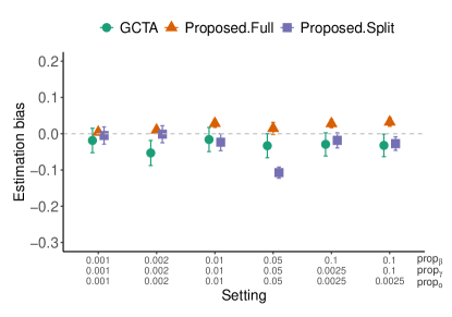
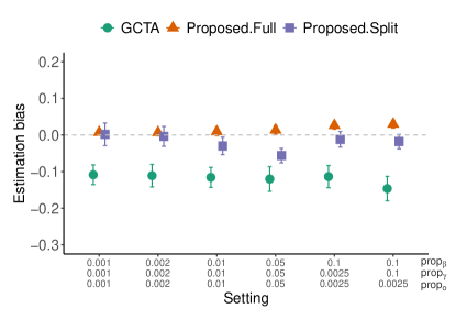
(a) Normal coefficients, linear models	(b) LDAK 1, linear models
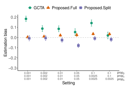
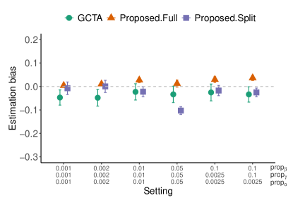
(c) LDAK 2, linear models	(d) Single mis-specified composite model

Figure 1: Comparison of estimation accuracy for four different genetic models when both traits are measured on the same set of individuals ($N_{y}=N_{z}=8000$). Each point represents the mean of the average bias, with error bars representing the standard error on both sides.

Estimation errors: The results of estimation accuracy when both traits are measured on the same set of individuals (overlapping samples) are present in Figure 1. Under correct linear model specifications with different effect distributions, Figures 1 (a), (b) and (c) show the proposed methods provide approximately unbiased estimates of genetic covariance when two models are not highly polygenic, not sensitive to the underlying effect distribution. The full-sample estimator and split-sample estimator are almost unbiased when both traits have sparse or moderate polygenic signals. Even if one trait is highly polygenic $(\mathrm{prop}=0.1)$, both estimators still provide satisfactory estimates of the genetic covariance. In addition, when both traits are highly polygenic $(\mathrm{prop}_{\beta},\mathrm{prop}_{\gamma})=(0.1,0.1)$, the estimation is still accurate if the genetic covariance is due to the shared variants with large effect sizes $(\mathrm{prop}_{o}=0.0025).$ As a comparison, the estimates from GCTA could be biased downward (Figure 1 (b) ) or upward (Figure 1 (c)) when the distributions of effect sizes depend on MAF and LD.

The full-sample estimator and the split-sample estimator have their own strengths and limitations. Consistent with the theoretical analysis, the split-sample estimator has a smaller bias under unbalanced sparsity settings, i.e. one trait is highly polygenic while the other trait is sparse with $(\mathrm{prop}_{\beta},\mathrm{prop}_{\gamma},\mathrm{prop}_{o})=(0.1,0.0025,0.0025)$. We provide more results in Figure S6 of the supplementary material to highlight this point. On the other hand, the full-sample estimator has better empirical performance when the genetic covariance is contributed by weak and dense effects $(\mathrm{prop}_{\beta},\mathrm{prop}_{\gamma},\mathrm{prop}_{o})=(0.05,0.05,0.05)$. In Section C of the Supplemental Materials, we further investigate the different behaviors using oracle estimators in linear models, which suggests that the difference in performance is related to the correlation between the error terms in the trait models.

Figure 1 (d) shows both methods give accurate estimations of the true genetic covariance under single model mis-specification, which is explained by Corollary 1 that the narrow-sense genetic covariance is equal to the true genetic covariance when only one model is mis-specified.

Coverage of confidence intervals: Furthermore, in Figure 2, we compare the coverage probabilities and the length of the confidence interval. When the distributional assumption is violated, the coverage probabilities of GCTA are low due to their biased estimation. For the split-sample method, the coverage probabilities of the confidence intervals are close to the nominal level when at least one trait has sparse signals. The results support our argument that the proposed method does not require both models to have sparse coefficients for valid inference.

The full-sample approach has coverage probabilities close to the nominal level when both trait models are sparse, while its performance gets worse when the bias dominates over the variance term in the unbalanced sparsity or dense effects setting. Therefore we provide a bias-adjusted confidence interval estimation based on theoretical results (Celentano et al., 2020; Tibshirani and Taylor, 2012) and evaluate its performance. We quantify the bias by $\hat{R}$ based on the prediction risk and residuals, and propose the following adjusted confidence interval,

$$CI(\alpha)=\begin{cases}[\widehat{I}_{\text{full}}-z_{1-\alpha/2}\widehat{\sigma}-\widehat{R},\widehat{I}_{\text{full}}+z_{1-\alpha/2}\widehat{\sigma}]&\text{ if }\widehat{R}>0\\ [\widehat{I}_{\text{full}}-z_{1-\alpha/2}\widehat{\sigma},\widehat{I}_{\text{full}}+z_{1-\alpha/2}\widehat{\sigma}-\widehat{R}]&\text{ if }\widehat{R}<0\end{cases}.$$ (18)

More details on the derivation of $\hat{R}$ can be found in Section C of the Supplemental Materials. Figure 2 shows the adjusted CI leads to valid coverage even when the effects are highly polygenic, while maintaining a shorter width than the estimate from GCTA method in most cases.

Finally, if one model is mis-specified, our proposed method still performs well. These results support our conclusion that the inference of genetic covariance between the linear trait and the nonlinear trait is robust to the mis-specification of the nonlinear function.

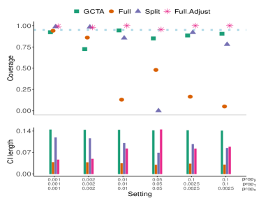
(a) Normal coefficients, linear models	(b) LDAK 1, linear models
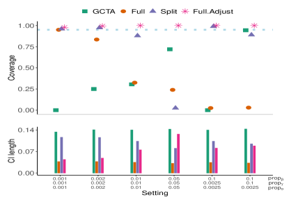
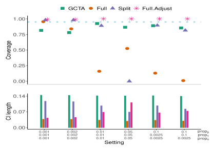
(c) LDAK 2, linear models	(d) Single mis-specified composite model

Figure 2: Comparison of coverage probability and confidence interval (CI) length when both traits are measured on the same set of individuals ($N_{y}=N_{z}=8000$). Conservative CI is constructed for the full-sample approach. The coverage probability results are reported in the upper panel and the corresponding average confidence interval length results are demonstrated by the bar plots in lower panel.

Non-overlapping setting: Results when the two traits are measured on two independent sets of individuals are given in Figure S1 and S2 in the Supplemental Materials. The split-sample and full-sample estimators have similar estimation biases and the bias is smaller when the effects are sparse (Figure S1). However, when the models are very polygenic, the full-sample approach has low coverage probability due to a smaller variance. In contrast, the split-sample approach gives better coverage (Figure S2). Similar estimation behaviors of two methods are observed under model mis-specification, and the proposed method is robust to model mis-specification (Figure S2 (b)-(d)).

4.2 Summary of additional simulations

In Supplemental materials, we include simulation results for binary traits and case-control designs (Figures S3-S4, Table S2). The results show the proposed method can still estimate the genetic covariance well. When the models are not highly polygenic, the coverage probabilities in Figure S4 are also close to the nominal level. In contrast, GCTA seems to have a large estimation bias for the genetic covariance even under the models with normal coefficients (Figure S3 (a)), resulting in low coverage probabilities in some cases. When one model is misspecified, GCTA estimation results in a larger bias (Figure S3 (d)). This may be due to the wrong working models fitted by GCTA-GREML for the binary traits.

We also evaluate the performance when causal variants are not independent in Figure S5. The proposed methods still perform well. When compared with the models with independent causal variants as shown in Figure 1, the estimates from GCTA have a larger bias when the signals are sparse, leading to lower corresponding coverage probabilities.

5 Real data application

We analyze the outbred Carworth Farms White (CFW) mice data set (Parker et al., 2016) to study the genetic covariance between various behavioral and physiological traits. Each CFW mouse was phenotyped for behavioral traits, bone and muscle traits, and other physiological traits, including fasting glucose levels, body weight, tail length and testis weight. The behavioral traits consist of conditioned fear, methamphetamine (MA) sensitivity and prepulse inhibition phenotypes. The bone or muscle traits include the weight of five hindlimb muscles and bone mineral density. Besides, a binary trait that signals abnormally high bone mineral density is generated. For each of the continuous phenotypes, we adjust for baseline weight, experimenters, sacrifice age and 1st PC of genotypes and normalize the residuals. After the pre-processing, the data set consists of 1038 mice with 79,824 genetic variants (SNPs), 66 continuous phenotypes and one binary trait. The data set includes various levels of missingness $(22\sim 211)$ in the trait values. The observations with missing traits are not used in the GLM fitting, but they are used in estimating the genetic covariance using the imputed trait values.

The phenotypic correlations among the continuous traits are shown in Figure 3 (a). The heritability estimates of continuous traits using GCTA and our proposed method are present in Figure 3 (b). Due to the limited sample size, the proposed method may not be able to capture the signal when traits have dense and weak effects. For the subsequent analysis, we consider 22 continuous traits with estimated heritability larger than 0.10 by the proposed method.

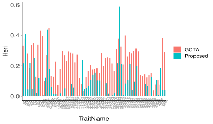
(a) Phenotype correlations among different traits.	(b) Estimated heritability of different traits.
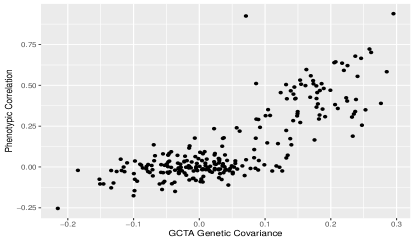
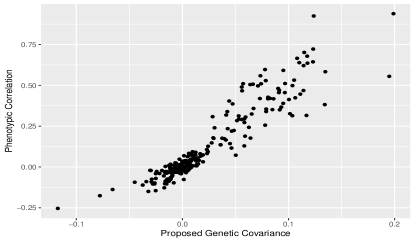
(c) GCTA estimator	(d) Proposed estimator
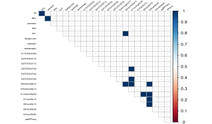
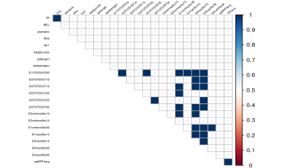
(e) GCTA estimator (Bonferroni)	(f) Proposed estimator (Bonferroni)

Figure 3: Results from analysis of the mouse GWAS data. (a) Phenotype correlations of 66 continuous traits; (b) Estimated heritability by GCTA method and the proposed method; (c)-(d) Scatter plots of phenotypic covariance and the estimated genetic covariance using GCTA ( and the proposed estimator for each pair of continuous traits with the estimated heritability larger than $0.1$; (e) -(f) Identified significant pair of traits with Bonferroni correction at the level of $0.05$ using GCTA estimator and the proposed estimator. There are 12 pairs identified by GCTA and 27 pairs identified using the proposed method.

5.1 Genetic covariance among different traits

To illustrate our method, we present the genetic covariance analysis for four selected traits. For the muscle traits, we choose the continuous trait extensor digitorum longus (EDL) and the binary trait signaling abnormal bone. Other traits include the physiological trait of testis weight, the MA sensitivity trait of the distance traveled, 0–30 min, on day 3 of methamphetamine sensitivity tests. For each selected trait, we calculate its genetic covariance with all other traits. For the binary trait, the estimated genetic covariance is calculated based on the observed scale. Model fitting and estimation of $\hat{\beta}$ and $\hat{\gamma}$ are implemented using the package glmnet with 10-fold cross-validation.

The genetic covariance results for the four traits are summarized in Figure 4 (a) - (d). For continuous traits, we report the bias-adjusted confidence interval in (18). Figure 4 (a) shows that the testis weight has no significant genetic covariance with other continuous traits. Figure 4 (b) suggests that the abnormal bone trait may be mainly related to the muscle traits. The scale of the genetic covariance is small because the abnormal bone trait is binary. In Figure 4 (c), the muscle trait EDL has a significant genetic covariance with other muscle traits like TA but does not have a shared genetic architecture with behavior traits. This agreed with the pleiotropy effects among the muscle traits (Parker et al., 2016). In Figure 4 (d), the MA sensitivity trait is closely related to other MA sensitivity behavior traits measure on Day 1 and 2 and is not related with trait measured on the third day. This result is reasonable because the mice were injected with saline on first two days and received MA on the third day so the activity on the day 3 should be less related to the baseline measurement on day 1 and 2.

These results show that our proposed estimator of genetic covariance works well for both continuous and binary traits. The results further confirm that many behavior-related traits share common genetic variants and physiological traits also share genetic effects. However, the genetic covariance between physiological traits and behavioral traits is small.

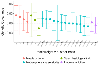
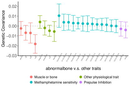
(a) Physiological trait, testis weight.	(b) Binary bone trait, abnormal bone.
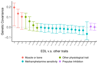
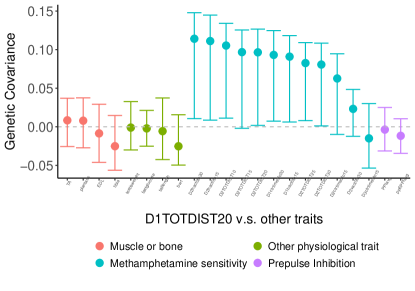
(c) Muscle trait	(d) Methamphetamine sensitivity trait
weight of extensor digitorum longus muscle.	the distance traveled, 0–20 min.

Figure 4: Estimated genetic covariance of four selected traits with other traits, where bars represent the confidence intervals. For continuous traits, we report the conservative adjusted confidence interval. The confidence level $\alpha$ is determined by Bonferroni correction $0.05/21$.

5.2 Comparison with GCTA and LDSC estimates

We compare the estimates of genetic covariance from the proposed method, GCTA and the LD-score regression. The scatter plots in Figure 3 (c)-(d) show the relationship between estimated genetic covariance and the observed phenotypic covariance. When the phenotypic correlation is around $0$, the proposed method gives estimates of the genetic covariance around $0.$ However, the estimates from GCTA could be from $-0.2$ to $0.15$, leading to inflated estimates. GCTA and LDSC estimations for four selected traits above are given in Figure S7 and S8. Additional comparisons of genetic covariance estimates by three methods are given in Figure S9.

We also compare the performances for identifying the non-zero genetic covariance based on the confidence interval estimation with Bonferroni correction for multiple comparisons (see Figure 3). The bias-adjusted confidence interval is used for the proposed method. Our method has identified more trait pairs (27 pairs) than GCTA (12 pairs) with a significant genetic covariance. The proposed method identifies more pairs related to the traveling distance traits measured in MA sensitivity experiments. Finally, as shown by Figure S10, the LDSC method only detect 6 pairs due to the fact that it uses summary statistics only.

6 Discussion

This paper proposes a general regression-based estimation and inference procedure for the genetic covariance and the narrow-sense genetic covariance based on GWAS data. The proposed estimator enjoys asymptotic normality under proper conditions and is robust to model mis-specifications. Numerical studies are conducted to explore its empirical performance under various sparsity levels. The accuracy of the proposed regression-based method depends on the precision of the fitted model and it works best under uncertain sparsity conditions, outperforming the random-effects model-based estimation. The proposed method may underestimate the true genetic covariance when it is contributed by weak and dense effects, in which case the fitted model would be inaccurate for limited sample sizes. In numerical experiments, we also find the robustness of the full-sample estimator outside the sparsity regime. Further theoretical investigation would be interesting.

The proposed estimator $\widehat{I}$ in (8) only uses the predicted trait values and residuals. We consider the $\ell_{1}$-penalized regression in (5) and (6) for its convenience in prediction and estimation, and its theoretical guarantees under the sparsity assumptions. It is however, possible to apply other appropriate penalties or more flexible machine learning methods in the first step. Such machine learning approaches can be theoretically justified if at least one model provides accurate predictions as studied in the double machine learning literature (Chernozhukov et al., 2018).

The practical implementation of the proposed methods for large-scale genotype data involves an efficient implementation of penalized GLM regression, which has been shown to be feasible for the UK Biobank genotype data (Privé et al., 2019; Qian et al., 2020). Computational tricks such as using marginal association statistics or well-designed iteration rules have been applied to improve efficiency. The tuning parameter selection using cross-validation is computationally intensive. Further exploration of other efficient tuning parameter selection methods for GLMs is warranted.

FUNDING

This research was supported by NIH grants R01GM123056 and R01GM129781. Sai Li’s research was also supported by the Fundamental Research Funds for the Central Universities, and the Research Funds of Renmin University of China.

SUPPLEMENTARY MATERIAL

Supplement to “A Regression-based Approach to Robust Estimation and Inference for Genetic Covariance”. In the Supplementary Materials, we provide the proofs of theorems, more discussions on estimation bias and imputation, and more results for numerical experiments and data applications.

References

- Bulik-Sullivan et al. (2015) Bulik-Sullivan, B., H. K. Finucane, V. Anttila, A. Gusev, F. R. Day, P.-R. Loh, L. Duncan, J. R. Perry, N. Patterson, E. B. Robinson, et al. (2015). An atlas of genetic correlations across human diseases and traits. Nature genetics 47(11), 1236–1241.
- Cai and Guo (2020) Cai, T. T. and Z. Guo (2020). Semisupervised inference for explained variance in high dimensional linear regression and its applications. Journal of the Royal Statistical Society Series B 82(2), 391–419.
- Celentano et al. (2020) Celentano, M., A. Montanari, and Y. Wei (2020). The lasso with general gaussian designs with applications to hypothesis testing. arXiv preprint arXiv:2007.13716.
- Chernozhukov et al. (2018) Chernozhukov, V., D. Chetverikov, M. Demirer, E. Duflo, C. Hansen, W. Newey, and J. Robins (2018, 01). Double/debiased machine learning for treatment and structural parameters. The Econometrics Journal 21(1), C1–C68.
- Cross-Disorder Group of the Psychiatric Genomics Consortium (2019) Cross-Disorder Group of the Psychiatric Genomics Consortium (2019). Genomic relationships, novel loci, and pleiotropic mechanisms across eight psychiatric disorders. Cell 179(7), 1469–1482.
- Evans et al. (2018) Evans, L. M., R. Tahmasbi, S. I. Vrieze, G. R. Abecasis, S. Das, S. Gazal, D. W. Bjelland, T. R. De Candia, H. R. Consortium, M. E. Goddard, et al. (2018). Comparison of methods that use whole genome data to estimate the heritability and genetic architecture of complex traits. Nature genetics 50(5), 737–745.
- Gazal et al. (2017) Gazal, S., H. K. Finucane, N. A. Furlotte, P.-R. Loh, P. F. Palamara, X. Liu, A. Schoech, B. Bulik-Sullivan, B. M. Neale, A. Gusev, et al. (2017). Linkage disequilibrium–dependent architecture of human complex traits shows action of negative selection. Nature genetics 49(10), 1421–1427.
- Gazal et al. (2019) Gazal, S., C. Marquez-Luna, H. K. Finucane, and A. L. Price (2019). Reconciling s-ldsc and ldak functional enrichment estimates. Nature genetics 51(8), 1202–1204.
- Guo et al. (2019) Guo, Z., W. Wang, T. T. Cai, and H. Li (2019). Optimal estimation of genetic relatedness in high-dimensional linear models. Journal of the American Statistical Association 114(525), 358–369.
- Janson et al. (2017) Janson, L., R. F. Barber, and E. Candes (2017). Eigenprism: inference for high dimensional signal-to-noise ratios. Journal of the Royal Statistical Society: Series B (Statistical Methodology) 79(4), 1037–1065.
- Lee et al. (2013) Lee, S. H., S. Ripke, B. M. Neale, S. V. Faraone, S. M. Purcell, R. H. Perlis, B. J. Mowry, A. Thapar, M. E. Goddard, J. S. Witte, et al. (2013). Genetic relationship between five psychiatric disorders estimated from genome-wide snps. Nature genetics 45(9), 984.
- Lee et al. (2012) Lee, S. H., J. Yang, M. E. Goddard, P. M. Visscher, and N. R. Wray (2012). Estimation of pleiotropy between complex diseases using single-nucleotide polymorphism-derived genomic relationships and restricted maximum likelihood. Bioinformatics 28(19), 2540–2542.
- Li et al. (2015) Li, Y. R., J. Li, S. D. Zhao, and et al. (2015). Meta-analysis of shared genetic architecture across ten pediatric autoimmune diseases. Nature Medicine 21, 1018–1027.
- Loh and Wainwright (2015) Loh, P.-L. and M. J. Wainwright (2015). Regularized m-estimators with nonconvexity: Statistical and algorithmic theory for local optima. The Journal of Machine Learning Research 16(1), 559–616.
- Negahban et al. (2012) Negahban, S. N., P. Ravikumar, M. J. Wainwright, B. Yu, et al. (2012). A unified framework for high-dimensional analysis of -estimators with decomposable regularizers. Statistical science 27(4), 538–557.
- Nelder and Wedderburn (1972) Nelder, J. A. and R. W. Wedderburn (1972). Generalized linear models. Journal of the Royal Statistical Society: Series A (General) 135(3), 370–384.
- Parker et al. (2016) Parker, C. C., S. Gopalakrishnan, P. Carbonetto, N. M. Gonzales, E. Leung, Y. J. Park, E. Aryee, J. Davis, D. A. Blizard, C. L. Ackert-Bicknell, et al. (2016). Genome-wide association study of behavioral, physiological and gene expression traits in outbred cfw mice. Nature genetics 48(8), 919–926.
- Privé et al. (2019) Privé, F., H. Aschard, and M. G. Blum (2019). Efficient implementation of penalized regression for genetic risk prediction. Genetics 212(1), 65–74.
- Privé et al. (2018) Privé, F., H. Aschard, A. Ziyatdinov, and M. G. Blum (2018). Efficient analysis of large-scale genome-wide data with two r packages: bigstatsr and bigsnpr. Bioinformatics 34(16), 2781–2787.
- Qian et al. (2020) Qian, J., Y. Tanigawa, W. Du, M. Aguirre, C. Chang, R. Tibshirani, M. A. Rivas, and T. Hastie (2020). A fast and scalable framework for large-scale and ultrahigh-dimensional sparse regression with application to the uk biobank. PLoS genetics 16(10), e1009141.
- Searle (1961) Searle, S. (1961). Phenotypic, genetic and environmental correlations. Biometrics 17(3), 474–480.
- Speed et al. (2017) Speed, D., N. Cai, M. R. Johnson, S. Nejentsev, D. J. Balding, U. Consortium, et al. (2017). Reevaluation of snp heritability in complex human traits. Nature genetics 49(7), 986–992.
- Speed et al. (2012) Speed, D., G. Hemani, M. R. Johnson, and D. J. Balding (2012). Improved heritability estimation from genome-wide snps. The American Journal of Human Genetics 91(6), 1011–1021.
- Tenesa and Haley (2013) Tenesa, A. and C. S. Haley (2013). The heritability of human disease: estimation, uses and abuses. Nature Reviews Genetics 14(2), 139–149.
- Tibshirani and Taylor (2012) Tibshirani, R. J. and J. Taylor (2012). Degrees of freedom in lasso problems. The Annals of Statistics 40(2), 1198–1232.
- Van de Geer et al. (2014) Van de Geer, S., P. Buhlmann, Y. Ritov, R. Dezeure, et al. (2014). On asymptotically optimal confidence regions and tests for high-dimensional models. The Annals of Statistics 42(3), 1166–1202.
- Verzelen and Gassiat (2018) Verzelen, N. and E. Gassiat (2018). Adaptive estimation of high-dimensional signal-to-noise ratios. Bernoulli 24(4B), 3683–3710.
- Wang and Li (2022) Wang, J. and H. Li (2022). Estimation of genetic correlation with summary association statistics. Biometrika 109(2), 421–438.
- Yang et al. (2015) Yang, J., A. Bakshi, Z. Zhu, G. Hemani, A. A. Vinkhuyzen, S. H. Lee, M. R. Robinson, J. R. Perry, I. M. Nolte, J. V. van Vliet-Ostaptchouk, et al. (2015). Genetic variance estimation with imputed variants finds negligible missing heritability for human height and body mass index. Nature genetics 47(10), 1114–1120.