A Lightweight and Gradient-Stable Neural Layer

Abstract

We propose a neural-layer architecture based on Householder weighting and absolute-value activating, hence called Householder-absolute neural layer or simply Han-layer. Compared to a fully connected layer with $d$-neurons and $d$ outputs, a Han-layer reduces the number of parameters and the corresponding complexity from $O(d^{2})$ to $O(d)$. The Han-layer structure guarantees two desirable properties: (1) gradient stability (free of vanishing or exploding gradient), and (2) 1-Lipschitz continuity. Extensive numerical experiments show that one can strategically use Han-layers to replace fully connected (FC) layers, reducing the number of model parameters while maintaining or even improving the generalization performance. We will also showcase the capabilities of the Han-layer architecture on a few small stylized models, and discuss its current limitations.

1 Introduction

The advancement of neural networks has sparked a revolution across multiple disciplines. However, with the increasing complexity of the problems they are designed to solve, the models have become more cumbersome and computationally expensive. For example, the cost of training a large language model (LLM) can be in millions [1], and the number of parameters of such a model is often several billion. On the other hand, small-scale devices, such as mobile or vehicle-mounted devices, are resource-constrained, making it hard to deploy such colossal models. Consequently, there is a growing demand for leaner models that have fewer parameters and can operate more efficiently [1, 2]. Researchers have employed methods such as devising low-complexity operators, and compressing and pruning models, as demonstrated in recent surveys [2, 3].

So far, however, there is still a lack of widely used low-complexity layer architecture that can effectively replace fully connected layers (under suitable conditions, of course). In this paper, we propose a new neural network layer called the Householder absolute-value neural layer (or Han-layer), which replaces the dense weight matrix in a fully connected layer with a Householder matrix and uses the absolute-value function as the activation function. Our choice of Householder matrix is motivated by two key factors. First, it is an orthogonal matrix, ensuring the stability of gradients during training. Second, a $d\times d$ Householder matrix involves just $d$ parameters, thereby making it possible to yield a substantial reduction in the overall parameter count.

Furthermore, our selection of ABS as the activation function is guided by the following considerations. Firstly, the Jacobian matrix of ABS, when applied element-wise, is an orthogonal matrix with $\pm 1$ on its diagonal. By construction, deep network structures built with multiple Han-layers demand relatively few parameters and theoretically avoid the gradient vanishing or exploding problem. Therefore, our model obviates the need for employing normalization techniques and conventional residual connections [4, 5, 6, 7]. Additionally, ABS, as a piece-wise linear function, which can be viewed as a combination of two ReLU functions, has very low computational complexity.

1.1 Contributions

We propose a new, lightweight and gradient stable layer architecture called Han-layer, and carefully examine its properties. We conduct extensive experiments to evaluate the capabilities of neural networks equipped with multiple Han-layers (or simply HanNets for brevity). In addition, since Han-layers are 1-Lipschitz continuous, they are naturally resistant to adversarial attacks to a degree.

• On several standard datasets for regression and image classification, our experiments indicate that HanNets can significantly reduce the number of model parameters, even within models already characterized by lightweight, while maintaining, and in some cases improving, generalization performance.

• On stylized small problems (see Section 4), our experiments show the existence of some structured data on which HanNets can greatly outperform conventional Multi-layer Perceptrons (MLPs) in terms of generalization, as is demonstrated in Figure 1 where a HanNet shows remarkable superiority over traditional FCNets and produces a nearly perfect result.

(a) FCNet: 85.2% test accuracy.

(b) HanNet: 99.5% test accuracy.

Figure 1: Landscapes and top views from FC and Han models on the checkerboard set. (a) for FCNet, (b) for HanNet.

Even though our empirical results in this paper are not obtained from huge-scale models, they should be sufficient to establish that the new Han-layer architecture represents a useful technique to be included in the existing toolbox of deep learning.

1.2 Notations

We define a function $F_{L}$ from $\mathbb{R}^{m}\to\mathbb{R}^{n}$ realized by a deep neural network with depth $L$,

$$F_{L}(x,\textbf{W},\textbf{b}):=(\psi_{L}\circ\cdots\circ\psi_{1})(x),$$ (1)

where $\textbf{W}=\{W_{1},...,W_{L}\}$ and $\textbf{b}=\{b_{1},...,b_{L}\}$ is the collections of weight matrices and bias vectors, $\psi_{i}$ is the layer function, and if $\psi_{i}$ is a fully connected layer with activation function, then

$$\psi_{i}(\cdot)\equiv\psi_{i}(\cdot,W_{i},b_{i}):=\phi(W_{i}(\cdot)+b_{i}),$$ (2)

where $W_{i}$ is the weight matrix and $\phi(\cdot)$ is the element-wise activation function. The deep neural network (DNN) function $F_{L}(x,\textbf{W},\textbf{b})$ can be computed via forward propagation,

$$s_{0}=x;\;\;z_{k}=W_{k}s_{k-1}+b_{k},s_{k}=\phi(z_{k}),\;\;k=1,\cdots,L.$$ (3)

For the convenience of subsequent analysis, here we calculate the typical Jacobian matrix involved in the gradient computation through backpropagation, denoted as the $G$-matrix,

$$G_{L}(x,\textbf{W},\textbf{b})\equiv\frac{\partial F_{L}(x,\textbf{W},\textbf{b})}{\partial x}=\prod_{k=L}^{1}W_{k}\nabla\phi(z_{k}),$$ (4)

where $\nabla\phi(z_{k})$ is the diagonal, Jacobian matrix of $\phi(\cdot)$ evaluated component-wise at a vector $z_{k}$. The spectrum of a so-called $G_{L}$-matrix characterizes whether vanishing or exploding gradient would happen or not. Roughly speaking, $G_{L}$-matrix is the dominant part of the gradient. As $L\rightarrow\infty$, vanishing gradient corresponds to $\|G_{L}\|\rightarrow 0$ and exploding gradient to $\|G_{L}\|\rightarrow\infty$.

1.3 Related Work

1.3.1 Absolute-Value Function for Activation

In earlier periods of neural network research, piece-wise linear model structures were considered that involved ABS functions [8, 9]. However, ABS failed to gain mainstream popularity and was seldom utilized, e.g. not mentioned in this survey [10]. Instead, ReLU has become the most widely used activation function in recent years, as demonstrated in [11]. The author in [12] suggests using ABS activation in a “bidirectional neuron” architecture based on interpretability considerations. More recently, in [13], the authors show that under the same conditions, ABS can better resist the occurrence of “collapse to constant” and maintain network variability better than ReLU. Additionally, in [14], the author demonstrates that neural networks with absolute value activation functions can $\epsilon$-approximate functions that are analytic on certain regions. For more information about piecewise linear activations including the absolute-value function, see this survey [15].

1.3.2 Orthogonal Weight Matrix

Orthogonal weight-matrix initialization has been the subject of theoretical and empirical investigations and has proven to be useful in deep learning, that is, orthogonal initial weights can speed up convergence relative to standard Gaussian initial weights, as evidenced by studies such as [16, 17, 18, 19, 20]. Additionally, this orthogonal weight-matrix approach has been applied to recurrent and convolution neural networks to improve model performance, as shown in studies such as [21, 22, 23, 24, 25, 26, 27, 28, 29]. For example, the authors in [24] show that orthogonal neural networks have better generalization performance based on the local isometry property.

In this article, we mainly take advantage of orthogonality for gradient stability. In a neural network mapping from $\mathbb{R}^{d}$ to $\mathbb{R}^{d}$, if the Jacobian matrix of each layer function is orthogonal, then the total Jacobian matrix of the mapping will be orthogonal since products of orthogonal matrices remain orthogonal. Therefore, with all eigenvalues maintaining unit modulus, there will be no gradient explosion or vanishing.

Moreover, a simple method [30] to encourage near-orthogonal weight matrices in FCNets is to regularize each weight matrix $W$ by the term:

$$\|W^{{\intercal}}W-I\|_{F}^{2}\ \ \mathrm{or}\ \ \|WW^{{\intercal}}-I\|_{F}^{2},$$

where $I$ denotes the identity matrix. For a comparison purpose, we will use this regularization in some subsequent experiments, see Table 3.

1.3.3 Householder Weighting

The Householder reflection matrix associated with a nonzero vector $u\in\mathbb{R}^{d}$ is

$$H(u)=I-2\frac{uu^{{\intercal}}}{u^{{\intercal}}u},$$ (5)

where $I$ denotes the identity matrix in $\mathbb{R}^{d}$. This matrix is both symmetric and orthogonal. In addition, the number of parameters in $H(u)$ is an order of magnitude smaller than that of a general dense matrix.

In some works such as the orthogonal RNN (oRNN) [21], products of Householder reflection matrices are used to represent transition matrices to alleviate issues related to vanishing and exploding gradients. A more recent work in this direction is [31].

2 Introduction to Han-layer

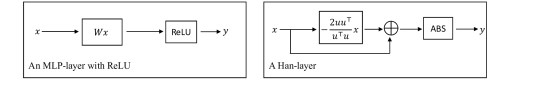
Figure 2: Visualization of An MLP-layer with ReLU activation function and a Han-layer. The $W$ is a weight matrix, $u$ is a nonzero vector, $\bigoplus$ denotes element-wise addition and ABS is the absolute-value function.

A Householder-absolute neural layer, or Han-layer, is composed of a Householder matrix followed by ABS activation,

$$\varphi(x;u,b):=\mathbf{ABS}\left(H(u)x+b\right),$$ (6)

which has a linear complexity. We will call a neural network mainly composed of Han-layers as a HanNet. Additionally, Figure 2 visually illustrates the distinction between a conventional MLP-layer and a Han-layer. It is interesting to note that our Han-layer can be seen as having an intrinsic residual connection.

2.1 Absolute-value Activating

We motivate element-wise absolute-value activating by considering a class of functions defined below.

Definition 1.

A function $\phi(t):\mathbb{R}\rightarrow\mathbb{R}$ has Property A if

1. $\phi$ is nonlinear and continuous in $\mathbb{R}$;

2. $\phi$ is differentiable in $\mathbb{R}$ except in a countable set $\mathcal{C}_{\phi}\subset\mathbb{R}$;

3. $\phi$ satisfies the following unit-derivative condition:

   $$|\phi^{\prime}(t)|=1,~{}~{}\forall t\in\mathbb{R}\setminus\mathcal{C}_{\phi}.$$ (7)

We restrict non-differentiability to a countable set to avoid unnecessary complications introduced by uncountable sets.

Nonlinearity, continuity and differentiability (almost everywhere) are universally required for activation functions with obvious or well-explained rationales [32]. Hence, conditions A1-A2 are natural.

It is easy to see that condition A3 is the necessary and sufficient condition for the element-wise function $\phi(x):\mathbb{R}^{d}\rightarrow\mathbb{R}^{d}$ to have an orthogonal Jacobian matrix. Therefore, to guarantee the orthogonality of the $G_{L}$-matrix in (4), we propose to impose the unit-derivative condition (7) on element-wise activation functions.

Lemma 1.

Let $\phi:\mathbb{R}\rightarrow\mathbb{R}$ have Property A and $|\mathcal{C}_{\phi}|$ denote the cardinality of $\mathcal{C}_{\phi}$. Then $|\mathcal{C}_{\phi}|\geq 1$.

We notice that $|\mathcal{C}_{\phi}|$ is the number of non-differentiable points. This result follows immediately from the observation that if $\mathcal{C}_{\phi}$ is empty, then $\phi$ would be differentiable on the entire line with a constant derivative and thus must be linear which would fail condition A1 (otherwise there would exist $t_{0}\in\mathbb{R}$ so that $\lim_{t\to t_{0}^{+}}\phi^{\prime}(t)\neq\lim_{t\to t_{0}^{-}}\phi^{\prime}(t)$).

Lemma 2.

Let $\phi:\mathbb{R}\rightarrow\mathbb{R}$ have Property A. Then $\phi$ is piecewise linear so that each piece has the functional form $\phi(t)=\pm t+\mathrm{const}$ with a different constant . In the case of the minimum cardinality $|\mathcal{C}_{\phi}|=1$ with $\mathcal{C}_{\phi}=\{\alpha\}$, $\phi$ has the functional form

$$\phi(t)=\pm|t-\alpha|+\mathrm{const}.$$ (8)

Proof.

The first part is obvious. When $\mathcal{C}_{\phi}=\{\alpha\}$, the functional form in each piece is $\phi=(t-\alpha)+\mathrm{const}$ or $-(t-\alpha)+\mathrm{const}$, then $\phi$ has the functional form $\phi(t)=\pm|t-\alpha|+\mathrm{const}$. ∎

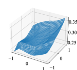
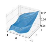
(a) Approximate FC-1. Left to right: the original FC-1, the trained FC-1, the trained Han-3.

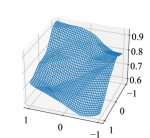
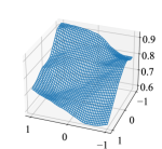
(b) Approximate Han-3. Left to right: the original Han-3, the trained FC-1, the trained Han-3.

Figure 3: Landscape of $\|F_{FC}(x)\|_{2}$ and $\|F_{Han}(x)\|_{2}$ in one instance, where $d=50$.

In a neural network with an element-wise activation function constructed from $\phi$ in (8), the sign will be absorbed by weights and the constants will be absorbed into bias terms. Therefore, without loss of generality (8) simply reduces to the absolute-value function. We summarize the most relevant facts as a proposition below, where without confusion we use $\phi$ inter-changeably with either the scalar case or its element-wise extension in $\mathbb{R}^{n}$.

Proposition 1.

Let $\phi(x):\mathbb{R}^{d}\rightarrow\mathbb{R}^{d}$ be an element-wise activation function. The Jacobian matrix of $\phi$ at $x\in\mathbb{R}^{n}$, which is diagonal if it exists, is orthogonal if and only $\phi$ satisfies the unit-derivative condition (7). Moreover, among all activation functions with Property A, the one with maximum differentiability is the absolute-value function $\phi(\cdot)=|\cdot|$.

3 Properties of HanNet

We demonstrate that the Han-layer function exhibits a Lipschitz constant of 1 and possesses a stable gradient. Furthermore, we conduct an experimental evaluation to mutually approximate Han and FC models, which validates the feasibility of replacing the FC-layer with Han-layers.

Proposition 2.

$\varphi(x;u,b)=|H(u)x+b|$ is a 1-Lipschitz function.

Proof.

$$\||H(u)x_{1}+b|-|H(u)x_{2}+b|\|_{2}$$ (9)

$$\leq \|H(u)x_{1}-H(u)x_{2}\|_{2}$$

$$\leq \|H(u)\|_{2}\|x_{1}-x_{2}\|_{2}$$

$$\leq \|x_{1}-x_{2}\|_{2}$$ (10)

which completes the proof. ∎

3.1 Gradient stability

Let the neural network function $F_{L}(x,\textbf{W},\textbf{b})$ be defined in (1). For HanNet, with the notation $\textbf{u}=\{u_{k}\}_{k=1}^{L}$ with all $u_{k}\neq 0$, the $G_{L}$-matrix takes the form

$$G_{L}(x,\textbf{u},\textbf{b})=\prod_{k=1}^{L}H(u_{k})\nabla\phi(z_{k}),\vspace{-.05cm}$$ (11)

where $H(u_{k})$ is defined by (5). Evidently, the diagonal matrices $\nabla\phi(z_{k})$ are orthogonal matrices whose diagonal elements are equal to $\pm 1$ (with the convention $|\phi^{\prime}(0)|=1$). Then the product $\prod_{k=1}^{L}H(u_{k})\nabla\phi(z_{k})$ is always orthogonal, which implies that the gradient will never vanish or explode. We state this fact as the following proposition.

Proposition 3.

The $G$-matrix for HanNet, that is, $G_{L}(x,\textbf{u},\textbf{b})$ defined in (11), remains orthogonal for any $x$, any u (with all $u_{k}\neq 0$), any b, and any integer $L>0$.

3.2 Mutual Approximation: FC and Han

We aim to empirically evaluate the efficacy of using Han-layers (of $O(d)$ complexity) to replace FC-layers (of $O(d)$ complexity), mainly to get an idea on how many Han-layers are needed to approximate one FC-layer. For this purpose, we define the following two models:

$$\textrm{FC-1}:=\psi_{out}\circ[\psi_{1}]\circ\psi_{in}(x),$$

$$\textrm{Han-k}:=\psi_{out}\circ[\varphi_{k}\circ...\circ\varphi_{1}]\circ\psi_{in}(x),$$

where $\psi_{in}$ ($\psi_{out}$) denotes an input (output) layer in both models. Model FC-1 has one hidden FC-layer $\psi_{1}$, and Han-$k$ composes of $k$ Han-layers $\varphi$, and the width of all hidden layers in both models is fixed at $d$. FC-1 uses ReLU as the activation function, while Han-$k$ uses ABS.

Specifically, we experiment with $k=3$ and $d$ is from 30 to 100. The number of model parameters in FC-1 ranges from 900 to 10000 roughly, while for Han-3 it is from 180 to 600 roughly. We randomly sample 2000 points from the square $(-1,1)^{2}$ as the training set, and 10000 points from the square for testing. All FC models are initialized using random orthogonal initialization. We use the mean squared error (MSE) loss function. Further experimental details are outlined in Table 1. In order to minimize the impact of training interventions on the final results, we explore a list of hyper-parameters to identify the best-performing model. Specifically, the initial learning rate is annealed to 0.2 for 6/10 and 9/10 of the training duration.

Table 1: Settings in mutual approximation experiments.

Optimizer	LR	weight decay	batch size	epochs
{SGD, Adam}	{0.0001, 0.001, 0.01, 0.1}	{0.0, 0.001}	100	1000

The experimental results are presented in Figures 3 and 4. We observe that the test errors of the two models fitting each other are around $10^{-3}$ or slightly below. The obtained landscapes are consistent with the original models, suggesting the potential for replacing FC-layers with a small number of Han-layers that is far fewer than width $d$.

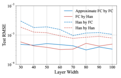
Figure 4: The average root mean squared error (RMSE) on 5 instances. Blue line: FC-1 approximates itself, red line: Han-3 approximates FC-1, blue dash line: FC-1 approximates Han-3, red dash line: Han-3 approximates itself.

Table 2: The test RMSE for input dimensions ranging from 2 to 4, where the width $d$ in all hidden layers is $d=100$.

	approximate FC-1		approximate Han-3
trained model	FC-1	Han-3	FC-1	Han-3
input dim 2	0.00033	0.00049	0.00107	0.00079
input dim 3	0.00086	0.00078	0.00251	0.00237
input dim 4	0.00184	0.00192	0.00478	0.00494

Moreover, we extend the input and output dimensions to 4 while maintaining $d=100$, and the results are summarized in Table 2. Our findings reveal that as the input data dimensionality increases, the RMSE values for both models also increase. However, the mutual approximation performance of the two models remains comparable. Overall, the above experiment confirms the ability of HanNet and FCNet to approximate each other, thereby shedding light on the possibility of reducing the number of model parameters.

4 Stylized Datasets

In this section, we first evaluate our approach on a synthetic checkerboard dataset, depicted in Figure 5, which consists of 6561 mesh points over the square $[-1,1]^{2}$. Our experiments confirm that achieving a perfect solution on this dataset using standard MLPs is extremely challenging.

Figure 5: Checkerboard datasets. The right figure is the training set (25%).

We adopt MSE loss and select SGD optimizer with a momentum of 0.9. Our model is trained using a batch size of 100 and 40000 iterations. To solve each test instance, we perform SGD with 10 distinct initial learning rates:

$$\{0.001,0.005,0.01,0.025,0.05,0.075,0.1,0.25,0.5,1\}$$

and select the best result as the output. Moreover, the initial learning rate is annealed by a factor of 5 at the fractions 1/2, 7/10, and 9/10 of the training durations.

Our experiments show HanNets possess an unusually high level of generalization ability in Figure 1. A HanNet outperforms FCNets significantly and produces a nearly perfect result.

We also compare various FCNets with HanNets (FCNets with skip connection were also compared, but did not yield better results than the FCNets). We generate more than 200 pairs of FCNets and HanNets, with widths ranging from 20 to 100 in increments of 10 and depths from 2 to 30. The test results are presented in Figure 6 in the form of a heat map.

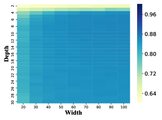
(a) FCNet: the best test accuracy is up to 87%.

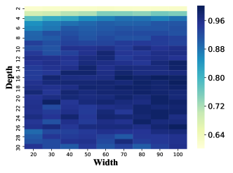
(b) HanNet: the best test accuracy is over 99%.

Figure 6: Heat maps of FCNets and HanNets.

The results in Figure 6 show that there is a significant gap in test accuracy between FCNets (around 85%) and HanNets (over 99%) for a wide range of test cases. The remarkable near-perfect results achieved by HanNets, without any explicit regularization, are both impressive and stable, as similar results can be obtained from other random 25% vs. 75% data splits. We also observe that over-parameterization is not a necessary condition for achieving near-zero test error, as demonstrated in one of the cases in Figure 6 (Bottom) where 400 parameters are sufficient.

4.1 A preliminary explanation

To explain HanNet’s exceptional performance on the checkerboard dataset, we take an intuitive viewpoint based on the amount of nonlinearity provided by different models. In most feed-forward networks, the main source of nonlinearity is from the applications of nonlinear activation functions. Given an MLP-layer that maps from $\mathbb{R}^{d}$ to $\mathbb{R}^{d}$, the number of activation-function applications is $d$, with $d^{2}$ parameters in weight matrix $W$. Consequently, the activation-function utilization rate is $1/d$ (i.e., $d$ versus $d^{2}$), which serves as a normalized measure of nonlinearity. In contrast, with $d$ parameters in $u$, our Han-layer has an activation-function utilization rate 1 (i.e., $d$ versus $d$). Therefore, several Han-layers together can potentially produce more nonlinearity than a single MLP layer can, while using far fewer parameters.

It is reasonable to argue that with more nonlinearity a HanNet would be better equipped than an FCNet to approximate complex shapes as in the checkerboard dataset and capture the underlying patterns. On the other hand, an FCNet, characterized by over-parameterization, may be able to readily fit training data by memorizing them, but still fail to fully discern the underlying patterns. This seems to explain well the observed generalization discrepancy in Figure 1.

4.2 Ablation Study on Checkerboard

We conducted an ablation study on a $100\times 20$ network framework with seven different configurations to investigate how much Householder weighting and ABS activating contribute to the remarkable results on the checkerboard dataset. Table 3 lists the results, where we used either Householder (HH) or fully connected (FC) layers with/without orthogonal regularization, and either ABS, ReLU, MaxMin or GroupSort [32] activation functions. The latter two can keep the gradient norm unchanged [32]. We obtained orthogonal FCNets (OrthFC) by regularizing each weight matrix $W$ as [30]:

$$\lambda\|W^{{\intercal}}W-I\|_{F}^{2},$$

where $\lambda=0.1$ in our experiments.

Table 3 suggests that Householder weighting and ABS activating are equally critical to the 99% generalization accuracy of the HanNet. Other activation functions influence the test performance badly as that happens on the Householder Layer. Furthermore, OrthFC cannot achieve the same accuracy as HanNet, although each of its weight matrices is orthogonal.

Table 3: Ablation study on a $100\times 20$ network framework: Effects of layer and activation types on performance. HH denotes Householder and FC denotes fully connected layers.

	Layer type			Activation type				Test accuracy
	HH	FC	OrthFC	ABS	ReLU	MaxMin	GroupSort (5)
(a)	✓	–	–	✓	–	–	–	99.2%
(b)	✓	–	–	–	✓	–	–	66.2%
(c)	✓	–	–	–	–	✓	–	77.6%
(d)	✓	–	–	–	–	–	✓	81.4%
(e)	–	✓	–	✓	–	–	–	85.3%
(f1)	–	–	✓	✓	–	–	–	86.7%
(f2)	–	–	✓	–	✓	–	–	75.5%

4.3 Another Stylized Dataset

The remarkable performance of HanNet on the checkerboard dataset is not an isolated case, as shown by the experiment in [33]. Here, we fit another function $g(x)$ using HanNet and FCNet, defined by the sum of two sine-products (of low and high frequencies)

$$g(x)=\sin(2\pi x_{1})\sin(2\pi x_{2})+\sin(10\pi x_{1})\sin(10\pi x_{2}),$$

where $x=(x_{1},x_{2})\in[0,1]^{2}$ is evaluated on the same grid as in the checkerboard dataset (also 25% of the data used for training). All models have a width of 200 and a depth of 20, and are trained with the same SGD optimizer and annealing strategy on checkerboard for 80000 iterations.

Figure 7: Landscapes and top views from FC and Han models. From left to right: the original data, HanNet, FC-ReLU, FC-ABS. The test loss by HanNet is 0.034 while it is about 0.37 by the other two models.

The results in Figure 7 demonstrate a clearly superior performance of HanNet over FCNet, indicating that the advantage of HanNet is not limited to the checkerboard dataset only. Of course, further study is needed to fully understand this advantage.

5 Experiments on Larger Datasets

We present extensive numerical experiments to convincingly demonstrate the efficacy of the Han model, using the following datasets.

We conduct an investigation into the impact of the Han model on a widely used MNIST dataset [34] and explored its robustness. We also evaluate the regression performance on five classic datasets, namely Bikesharing, Cal Housing, Elevators, Parkinsons, and Skillcraft [35, 36, 37, 38, 39]. In addition, we assess the performance of the proposed model on four widely used image classification datasets, namely CIFAR10, CIFAR100, STL10, and Downsampled-ImageNet [40, 41, 42], where the last one is a downsampled version of ImageNet for affordability reasons.

All training is performed using PyTorch [43] on a shared cluster. Multiple runs are performed for each test instance, starting with different random initializations of the model parameters. All reported values are the average of at least five runs.

5.1 MNIST Dataset

5.1.1 Same performance, fewer parameters

Our study aims to evaluate the model’s performance on MNIST dataset [34]. In this study, we consider one hidden layer FCNet model, and $k$ Han-layer models, where $k$ ranges from 2 to 20. Notably, the width of each layer is fixed to the input size ($784$) in two models. To train our models, we use 10,000 instances for training and the remaining instances for testing. The details of other hyperparameters used in this study are presented in Table 4. We anneal the initial learning rate to 0.2 during half of the training period.

Table 4: Settings on MNIST.

Optimizer	LR	loss	weight decay	batch size	epochs
Adam	0.001	cross entropy	0.001	256	100

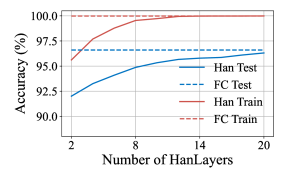
Figure 8: The train/test performance in 1 hidden layer FCNet and $k$-layer HanNets ($k$ from 1 to 20).

Figure 8 depicts that a 20-layer HanNet achieves the same train/test accuracy as FCNet on the clean dataset, while utilizing approximately $40K$ and $600K$ parameters, respectively.

5.1.2 Robustness by 1-Lipschitz

Many studies have established the robustness of 1-Lipschitz models against adversarial examples, for instance as evidenced by [44]. We investigate the contrast in robustness between Han and FC models using identical settings as in the previous subsection. The baseline models are one hidden layer FCNet with a width of 784, and a 20 hidden Han-layer model with the same width.

Adversarial examples are generated using PGD and CW attacks as detailed in [45, 46] and summarized in Table 5. We extend our evaluation to defensive FC models trained with adversarial training and TRADES [46, 47] using $\ell_{\infty}$ FGSM attack samples with a maximum perturbation of $\rho=0.1$, in addition to vanilla FCNet. To improve the robustness of HanNet, we adjust the value of weight decay in the optimizer and select the value from $\{0.01,0.05,0.1,0.2\}$ that offers the best robustness while maintaining clean accuracy above 0.9.

Table 5: Attack settings. $\rho$ is the maximum perturbation, $\alpha$ is the magnitude of the perturbation in each iteration, $c$ is the regularization constant value.

PGD $\ell_{\infty}$	30 steps , $\rho=0.1,0.2,0.3$, $\alpha=0.01$
PGD $\ell_{2}$	30 steps , $\rho=1.0,2.0,3.0$, $\alpha=0.1$
CW	1000 steps, $c=1,3,5$

Table 6 presents empirical evidence that suggests vanilla HanNet surpasses vanilla FCNet in robustness under attack, despite having a clean accuracy that is 0.04 lower than FCNet. Moreover, HanNet’s performance is comparable with that of defensive FC models and in certain instances, outperforms them. For instance, under CW attack with $c=5$, HanNet yields approximately 0.65 accuracy, while FCNets only achieve about 0.2 accuracy. The findings of our study demonstrate that HanNet can achieve robustness on par with defensive FCNet on the MNIST dataset under some attack situations.

Table 6: The robust accuracy with respect to CW and PGD attacks. VT and AT denote vanilla training and adversarial training respectively.

		HanNet	FCNet
		VT	VT	Trades	AT
clean		0.925	0.964	0.969	0.967
	c=1	0.887	0.684	0.828	0.815
	c=3	0.757	0.069	0.437	0.348
CW	c=5	0.653	0.032	0.216	0.176
	$\rho=1$	0.783	0.705	0.866	0.859
	$\rho=2$	0.529	0.121	0.448	0.412
PGD $\ell_{2}$	$\rho=3$	0.260	0.007	0.071	0.051
	$\rho=0.1$	0.753	0.467	0.861	0.867
	$\rho=0.2$	0.406	0.018	0.475	0.420
PGD $\ell_{\infty}$	$\rho=0.3$	0.075	0.001	0.042	0.041

5.2 Regression

We conduct experiments on these five real-world regression datasets in Table 7. We choose Adam [48] optimizer which seems to be the method of choice for several works in that area including [49] in Table 8.

Table 7: Dataset statistics: $N$ is the number of samples, and Dim is the dimension of data vectors.

	Datasets	Dim	$N$
Regression	Bikesharing	15	17379
	Cal Housing	8	20640
	Elevators	18	16599
	Parkinsons	20	5875
	Skillcraft	19	3338

Table 8: Adam parameters on Regression Datasets.

LR	weight decay	batch size	epochs
0.001	0.0	100	300

We compare the performance of a HanNet with two FCNets. Table 9 lists the relevant statistics for the 3 DNNs where depth refers to the number of hidden layers (there exist additional, data-size-dependent input/output layers). We see that in terms of parameter numbers FCNet1 and HanNet are comparable peers, while FCNet2 has about 15 times more parameters.

Table 9: RMSE and R-squared on regression datasets. Lower RMSE and higher R-squared mean better model performance.

		$\delta=0.8$			$\delta=0.2$
		HanNet	FCNet1	FCNet2	HanNet	FCNet1	FCNet2
	Depth $\times$ Width (#param)	20 $\times$ 200 (10.6K)	5 $\times$ 50 (10.9K)	5 $\times$ 200 (165K)	20 $\times$ 200 (10.6K)	5 $\times$ 50 (10.9K)	5 $\times$ 200 (165K)
RMSE	Bikesharing	0.218	0.241	0.223	0.311	0.498	0.344
	Calhousing	0.431	0.462	0.459	0.476	0.506	0.498
	Elevators	0.087	0.090	0.091	0.103	0.140	0.106
	Parkinsons	1.235	2.035	1.399	3.072	5.034	4.187
	Skillcraft	0.255	0.282	0.266	0.276	0.328	0.301
R-squared	Bikesharing	0.951	0.938	0.949	0.898	0.744	0.877
	Calhousing	0.813	0.786	0.788	0.772	0.743	0.75
	Elevators	0.878	0.869	0.869	0.832	0.671	0.823
	Parkinsons	0.986	0.963	0.982	0.917	0.777	0.845
	Skillcraft	0.546	0.455	0.507	0.477	0.266	0.383

We present test RMSE loss values and R-squared values in Table 9, where all values are averaged over 5 trials. Clearly, HanNet outperforms its “peer” FCNet1 by a notable margin, especially when fewer training samples are used, and is also better than FCNet2 which uses 15 times more parameters. We mention that the best test performance of HanNet is statistically the same as (or better than) that reported in [49] with an FCNet & NIT model that uses more than $800K$ parameters. Furthermore, with fewer parameters, HanNet appears less influenced by overfitting, as seen in Figure 9. Figures for all datasets in the three models are provided in Appendix.

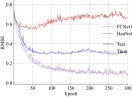
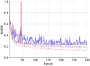
Figure 9: The train (solid line) and test (dotted line) RMSE on Bikesharing. Left: $\delta=0.2$; right: $\delta=0.8$. Red: for FCNet1; blue: for HanNet.

5.3 Use of Han-layers in Image Classification

In this section, we experiment on integrating Han-layers into existing models for image classification. First, we use Han-layers to replace some MLP-layers in MLP-Mixer models[50], and observe the resulting model performances. Next, we extend our investigation to a lightweight model, MobileViT [51].

5.3.1 Using Han-layers in MLP-Mixer

In literature, the term Multi-Layer Perceptron (MLP) is often used exchangeably with FCNet. Recently, MLP-dominated models have seen a wave of revivals for image recognition tasks [50, 52]. MLP-dominated models (without multi-head attention) are much more concise than Transformer-based models [53, 54] but can still maintain test performances on very large-scale datasets. The motivation of MLP-Mixer [50] is to use the purely fully connected layers to remove attention architectures. An MLP-Mixer block is the elementary unit in MLP-Mixer models that consists of several FC-layers and skip-connections to form the map from input $X$ to output $Y$ as is shown in Figure 10.

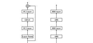
Figure 10: Two implementations of the channel mixing module using MLP-Mixer and Han-Mixer, respectively. HH denotes Householder.

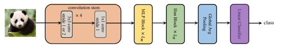
Figure 11: Overall structure of the tested Han/MLP-Mixer model ($L_{M}$ can be zero).

$$Z = X+\textbf{GELU}\left(W_{2}\ \textbf{Layer Norm}(W_{1}X)\right),$$ (12)

$$Y = Z+\textbf{GELU}\left(\textbf{Layer Norm}(ZW_{3})\ W_{4}\right),$$ (13)

where the first-row (12) is called token-mixing for cross-token communication, and the second-row (13) is called channel-mixing for cross-channel communication, both being of MLP structure. Here we form our Han-Mixer block by replacing all weight matrices $W_{i}$ by Householder matrices $H_{i}$, $i=1,2,3,4$, and all activation functions by the absolute function ABS, that is,

$$Z=\textbf{ABS}(H_{2}\textbf{ABS}(H_{1}X)),~{}~{}Y=\textbf{ABS}(\textbf{ABS}(ZH_{3})H_{4}),$$ (14)

where we remove skip connections and layer normalizations (since HanNets does not suffer from gradient problems). The resulting Han/MLP-Mixer models are shown in Figure 11, where we arrange some Han-Mixer blocks after MLP-Mixer blocks (which may be empty). The main reason for us to combine the two types of Mixer blocks is that, short of drastically increasing network width, Han-Mixers alone cannot always provide enough model parameters for large-scale datasets. In addition, we use the convolution stem recommended by [55] instead of the one in [50].

5.3.2 Settings

Table 10: The architecture on one MLP-block or Han-block. For simplification, in our experiments, all hidden MLP weights are square matrices.

	CIFAR	STL10	Downsampled-ImageNet
Patch size	$4\times 4$	$8\times 8$	$4\times 4$
Sequence Length	64	144	64
Channel number	512	512	1024

We summarize various configurations of each block on different data sets in Table 10. We run Mixers using the following number of layers {1, 2, 4, 8, 12, 16} and select the best one on each dataset. We use the convolution stem recommended by [55] instead of the one in [50]. Our convolutional stem designs use five layers, including four $3\times 3$ convolutions and a single $1\times 1$ final layer. The output channels are [64, 128, 256, 512, 512] on CIFAR10, CIFAR100 and STL10, and [128, 256, 512, 1024, 1024] on Downsampled-ImageNet. Some data augmentation methods are used, such as random HorizontalFlip, random augmentation[56], and Cutout[57]. For these datasets, we choose a modified Adam called AdamW [58]. Detailed settings are in Table 11 below.

Table 11: Dataset statistics and optimizer settings. $N$ is the number of samples, and Dim is the dimension of data vectors.

Dataset	Dim	$N$	LR	weight decay	batch size	epochs
CIFAR10/ CIFAR100	$3\times 32\times 32$	60000	0.001	0.1	256	600
STL10	$3\times 96\times 96$	13000			64	300
Downsampled-ImageNet	$3\times 32\times 32$	1331167			512	300

5.3.3 Results

In this section, we investigate HanNets’ generalization ability in image classification by comparing MLP-Mixers with our Han/MLP-Mixers presented in Subsection 5.3.1. The comparisons are made with 3 standard image datasets and a down-sampled version of ImageNet (due to computing source limitations).

Empirical evidence from MLP-based models [50] suggests that these models can achieve the state-of-the-art results on very large-scale datasets. Since the datasets used in our tests are not large enough to play to the full strengths of Mixer models, our aim here is not to observe how close our results can approach the state-of-the-art, but how Han-layer structures can impact the performance of Mixer models.

Table 12: Error rates (%) on STL10, CIFAR10, CIFAR100 and Downsampled-ImageNet datasets. On Downsampled-ImageNet, among MLPMixer ($i$) for $i=4,8,12,16$, $i=8$ gives the best results.

	#Param	STL10	CIFAR10	CIFAR100
CNN stem	1.82 M	18.2	7.2	27.8
+MLP (2)	2.89 M	18.2	5.3	27.2
+MLP (4)	3.96 M	18.7	5.5	27.1
+MLP (0) + Han (16)	1.86 M	15.3	5.9	26.7
+MLP (1) + Han (16)	2.39 M	16.7	5.0	24.6
+MLP (2) + Han (16)	2.93 M	17.1	4.7	24.4
+MLP (4) + Han (16)	4.00 M	17.8	4.6	24.7
ImageNet-Downsampled	#Param		Top1 error	Top5 error
CNN stem	8.28 M		55.7	31.2
+MLP (4)	16.7 M		44.2	21.2
+MLP (8)	27.2 M		42.6	20.2
+MLP (0) + Han (16)	8.35 M		48.9	26.1
+MLP (4) + Han (16)	16.8 M		41.1	19.2
WideResNet [42]	37.1 M		41.0	18.9

Table 12 reports test results from various MLP-Mixer and Han/MLP-Mixer models. On the smaller dataset STL10, HanMixers alone can already produce the best result. On larger datasets CIFAR10 and CIFAR100, enhanced performance from HanMixers is achieved either by adding a relatively few parameters (e.g., MLP (2) or (4) vs. MLP (2) or (4) + Han (16)), or even with far fewer parameters (e.g., MLP (4) vs. MLP (1)+Han (16)). On Downsampled-ImageNet, our Han/MLP-Mixer combination model clearly outperforms pure MLP-Mixers and offers a competitive performance with WideResNet [42] (41% Top1 error) while using only 40% parameters. In summary, the benefits of using Han-Mixers should be empirically evident according to these experiments.

5.4 Using Han-layers in MobileViT

In this section, we incorporate Han-layers into a lightweight vision transformer model, MobileViT [51], and compare model performance after MLP-layers are replaced by Han-layers. MobileViT combines convolutional and fully connected layers to achieve good performance while being lightweight. Details of this model, which are beyond the scope of this paper, can be found in [51].

In MobileViT [51], an MLP-block is of the form

$$Y=X+\textbf{Swish}\left(\textbf{Layer Norm}(X)W_{1}\right)W_{2},$$

which uses a layer normalization and Swish activation [59]. The above MLP-block is replaced, one-on-one, by the Han-block

$$Y=\textbf{ABS}(\textbf{ABS}(XH_{1})H_{2}),$$

where $H_{1}$ and $H_{2}$ are Householder matrices.

We experiment on two variants of the MobileViT model: MobileViT-XXS and MobileViT-XS with different sizes (see [51]). The training settings are similar to those in the previous MLP-Mixer experiments, except that we resize each image to $3\times 256\times 256$ according to the settings of MobileViT. Detailed settings are given in Table 13.

Table 13: Settings on the MobileViT experiments. Dim is the dimension of data vectors.

Dataset	Dim	LR	weight decay	batch size	epochs
CIFAR10/ CIFAR100	$3\times 256\times 256$	0.001	0.1	128	300
STL10				64

Testing performances of using MLP-blocks and Han-blocks are presented in Table 14. Across the three datasets (STL10, CIFAR10 and CIFAR100) and two model variants, the use of Han-blocks reduces the model parameter counts by approximately a half, while yielding comparable or better performance. These empirical findings again strongly support the use of Han-layers under suitable conditions.

Table 14: Error rates (%) on STL10, CIFAR10, CIFAR100 datasets, and on MobileViT-XXS and MobileViT-XS models.

MobileViT	Block	# Param	STL10	CIFAR10	CIFAR100
XXS	MLP	1.01 M	12.4	4.4	22.7
	Han	0.55 M	12.0	4.5	22.5
XS	MLP	2.00 M	11.5	4.2	21.1
	Han	0.97 M	11.0	3.9	20.4

6 Conclusions

We propose a lightweight layer structure (called Han-layer) for neural networks that has guaranteed gradient stability and 1-Lipschitz continuity. We provide extensive empirical evidence demonstrating the efficacy of Han-layers in reducing model parameters in certain neural networks. That is, when used strategically as substitutes for fully connected layers, a relatively small number of Han-layers can maintain or improve generalization performance. Moreover, we observe impressive generalization capabilities of HanNets on some synthetic datasets. These proof-of-concept results suggest that Han-layer can become a useful building block in constructing powerful deep neural networks. In the meantime, further investigations, especially theoretical ones, are still needed to fully assess the strength and weakness of Han-layers.

Since Householder matrices are square, as it is currently defined, a Han-layer cannot change dimensionality. Moreover, being light-weighted, Han-layers alone may not effectively provide enough parameters that are needed for building large models. Due to such limitations, Han-layers should be used strategically in combination with fully connected layers, and other suitable layer structures, to construct lean and effective deep neural networks in applications.

7 Acknowledgments

The work is supported by Shenzhen Research Institute of Big Data, and Shenzhen Science and Technology Program (Grant Number GXWD20201231105722002-20200901175001001)

Appendix A Other Figures on Regression Datasets

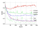
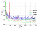
(a) Bikesharing

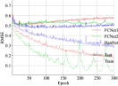
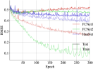
(b) Calhousing

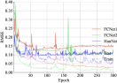
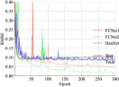
(c) Elevators

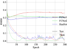
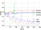
(d) Skillcraft

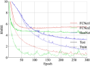
(e) Parkinsons

Figure 12: The train (solid line) and test (dotted line) RMSE on 5 regression datasets. Left: $\delta=0.2$; right: $\delta=0.8$. Red: for FCNet1; green: for FCNet2; blue: for HanNet.

References

- [1] E. Strubell, A. Ganesh, A. McCallum, Energy and policy considerations for deep learning in nlp, in: Proceedings of the 57th Annual Meeting of the Association for Computational Linguistics, 2019, pp. 3645–3650.
- [2] S. Khan, M. Naseer, M. Hayat, S. W. Zamir, F. S. Khan, M. Shah, Transformers in vision: A survey, ACM Computing Surveys (CSUR) (2021).
- [3] T. Liang, J. Glossner, L. Wang, S. Shi, X. Zhang, Pruning and quantization for deep neural network acceleration: A survey, Neurocomputing 461 (2021) 370–403.
- [4] S. Ioffe, C. Szegedy, Batch normalization: Accelerating deep network training by reducing internal covariate shift, in: F. Bach, D. Blei (Eds.), Proceedings of the 32nd International Conference on Machine Learning, Vol. 37 of Proceedings of Machine Learning Research, PMLR, Lille, France, 2015, pp. 448–456.
- [5] T. Salimans, D. P. Kingma, Weight normalization: A simple reparameterization to accelerate training of deep neural networks, arXiv preprint arXiv:1602.07868 (2016).
- [6] K. He, X. Zhang, S. Ren, J. Sun, Deep residual learning for image recognition, in: Proceedings of the IEEE Conference on Computer Vision and Pattern Recognition (CVPR), 2016.
- [7] A. Zaeemzadeh, N. Rahnavard, M. Shah, Norm-preservation: Why residual networks can become extremely deep?, IEEE transactions on pattern analysis and machine intelligence 43 (11) (2020) 3980–3990.
- [8] R. Batruni, A multilayer neural network with piecewise-linear structure and back-propagation learning, IEEE Transactions on Neural Networks 2 (3) (1991) 395–403.
- [9] J.-N. Lin, R. Unbehauen, Canonical piecewise-linear approximations, IEEE Transactions on Circuits and Systems I: Fundamental Theory and Applications 39 (8) (1992) 697–699.
- [10] A. Jagtap, G. E. Karniadakis, How important are activation functions in regression and classification? a survey, performance comparison, and future directions, Journal of Machine Learning for Modeling and Computing (2022).
- [11] V. Nair, G. E. Hinton, Rectified linear units improve restricted boltzmann machines, in: Icml, 2010.
- [12] A. Karnewar, Aann: Absolute artificial neural network, in: 2018 3rd International Conference for Convergence in Technology (I2CT), IEEE, 2018, pp. 1–6.
- [13] Y. Zhang, Y. Yu, Variability of artificial neural networks, arXiv preprint arXiv:2105.08911 (2021).
- [14] A. Beknazaryan, Analytic function approximation by path norm regularized deep networks, arXiv preprint arXiv:2104.02095 (2021).
- [15] Q. Tao, L. Li, X. Huang, X. Xi, S. Wang, J. A. Suykens, Piecewise linear neural networks and deep learning, Nature Reviews Methods Primers 2 (1) (2022) 42.
- [16] W. Hu, L. Xiao, J. Pennington, Provable benefit of orthogonal initialization in optimizing deep linear networks, in: International Conference on Learning Representations, 2020.
- [17] L. Huang, X. Liu, B. Lang, A. Yu, Y. Wang, B. Li, Orthogonal weight normalization: Solution to optimization over multiple dependent stiefel manifolds in deep neural networks, in: Proceedings of the AAAI Conference on Artificial Intelligence, Vol. 32, 2018.
- [18] Q. V. Le, N. Jaitly, G. E. Hinton, A simple way to initialize recurrent networks of rectified linear units, arXiv preprint arXiv:1504.00941 (2015).
- [19] J. Pennington, S. Schoenholz, S. Ganguli, The emergence of spectral universality in deep networks, in: International Conference on Artificial Intelligence and Statistics, PMLR, 2018, pp. 1924–1932.
- [20] L. Xiao, Y. Bahri, J. Sohl-Dickstein, S. Schoenholz, J. Pennington, Dynamical isometry and a mean field theory of cnns: How to train 10,000-layer vanilla convolutional neural networks, in: International Conference on Machine Learning, PMLR, 2018, pp. 5393–5402.
- [21] Z. Mhammedi, A. Hellicar, A. Rahman, J. Bailey, Efficient orthogonal parametrisation of recurrent neural networks using householder reflections, in: International Conference on Machine Learning, PMLR, 2017, pp. 2401–2409.
- [22] J. Wang, Y. Chen, R. Chakraborty, S. X. Yu, Orthogonal convolutional neural networks, in: Proceedings of the IEEE/CVF Conference on Computer Vision and Pattern Recognition, 2020, pp. 11505–11515.
- [23] M. Arjovsky, A. Shah, Y. Bengio, Unitary evolution recurrent neural networks, in: International conference on machine learning, PMLR, 2016, pp. 1120–1128.
- [24] K. Jia, S. Li, Y. Wen, T. Liu, D. Tao, Orthogonal deep neural networks, IEEE Transactions on Pattern Analysis & Machine Intelligence (01) (2019) 1–1.
- [25] J. M. Tomczak, M. Welling, Improving variational auto-encoders using householder flow, arXiv preprint arXiv:1611.09630 (2016).
- [26] E. Vorontsov, C. Trabelsi, S. Kadoury, C. Pal, On orthogonality and learning recurrent networks with long term dependencies, in: International Conference on Machine Learning, PMLR, 2017, pp. 3570–3578.
- [27] S. Wisdom, T. Powers, J. R. Hershey, J. Le Roux, L. E. Atlas, Full-capacity unitary recurrent neural networks, in: NIPS, 2016.
- [28] J. Zhang, Q. Lei, I. Dhillon, Stabilizing gradients for deep neural networks via efficient svd parameterization, in: International Conference on Machine Learning, PMLR, 2018, pp. 5806–5814.
- [29] S. Singla, S. Singla, S. Feizi, Improved deterministic l2 robustness on cifar-10 and cifar-100, in: International Conference on Learning Representations, 2021.
- [30] A. Brock, T. Lim, J. Ritchie, N. Weston, Neural photo editing with introspective adversarial networks, in: International Conference on Learning Representations, 2017.
- [31] A. Mathiasen, F. Hvilshøj, One reflection suffice, arXiv preprint arXiv:2009.14554 (2020).
- [32] C. Anil, J. Lucas, R. Grosse, Sorting out lipschitz function approximation, in: International Conference on Machine Learning, PMLR, 2019, pp. 291–301.
- [33] Q. Hong, Q. Tan, J. W. Siegel, J. Xu, On the activation function dependence of the spectral bias of neural networks, arXiv preprint arXiv:2208.04924 (2022).
- [34] Y. LeCun, L. Bottou, Y. Bengio, P. Haffner, Gradient-based learning applied to document recognition, Proceedings of the IEEE 86 (11) (1998) 2278–2324.
- [35] H. Fanaee-T, J. Gama, Event labeling combining ensemble detectors and background knowledge, Progress in Artificial Intelligence 2 (2) (2014) 113–127.
- [36] R. K. Pace, R. Barry, Sparse spatial autoregressions, Statistics & Probability Letters 33 (3) (1997) 291–297.
-
[37]
D. Dua, C. Graff, UCI machine learning
repository (2017).
URL http://archive.ics.uci.edu/ml - [38] M. Little, P. McSharry, S. Roberts, D. Costello, I. Moroz, Exploiting nonlinear recurrence and fractal scaling properties for voice disorder detection, Nature Precedings (2007) 1–1.
- [39] J. J. Thompson, M. R. Blair, L. Chen, A. J. Henrey, Video game telemetry as a critical tool in the study of complex skill learning, PloS one 8 (9) (2013) e75129.
- [40] A. Krizhevsky, G. Hinton, et al., Learning multiple layers of features from tiny images, Tech. rep., University of Toronto (2009).
- [41] A. Coates, A. Ng, H. Lee, An analysis of single-layer networks in unsupervised feature learning, in: Proceedings of the fourteenth international conference on artificial intelligence and statistics, JMLR Workshop and Conference Proceedings, 2011, pp. 215–223.
- [42] P. Chrabaszcz, I. Loshchilov, F. Hutter, A downsampled variant of imagenet as an alternative to the cifar datasets, arXiv preprint arXiv:1707.08819 (2017).
- [43] A. Paszke, S. Gross, F. Massa, A. Lerer, J. Bradbury, G. Chanan, T. Killeen, Z. Lin, N. Gimelshein, L. Antiga, et al., Pytorch: An imperative style, high-performance deep learning library, Advances in Neural Information Processing Systems 32 (2019) 8026–8037.
- [44] Y. Tsuzuku, I. Sato, M. Sugiyama, Lipschitz-margin training: Scalable certification of perturbation invariance for deep neural networks, Advances in neural information processing systems 31 (2018).
- [45] N. Carlini, D. Wagner, Towards evaluating the robustness of neural networks, in: 2017 ieee symposium on security and privacy (sp), IEEE, 2017, pp. 39–57.
- [46] A. Madry, A. Makelov, L. Schmidt, D. Tsipras, A. Vladu, Towards deep learning models resistant to adversarial attacks, in: International Conference on Learning Representations, 2018.
- [47] H. Zhang, Y. Yu, J. Jiao, E. Xing, L. El Ghaoui, M. Jordan, Theoretically principled trade-off between robustness and accuracy, in: International conference on machine learning, PMLR, 2019, pp. 7472–7482.
- [48] D. P. Kingma, J. Ba, Adam: A method for stochastic optimization, in: ICLR (Poster), 2015.
- [49] M. Tsang, H. Liu, S. Purushotham, P. Murali, Y. Liu, Neural interaction transparency (nit): Disentangling learned interactions for improved interpretability., in: NeurIPS, 2018, pp. 5809–5818.
- [50] I. Tolstikhin, N. Houlsby, A. Kolesnikov, L. Beyer, X. Zhai, T. Unterthiner, J. Yung, D. Keysers, J. Uszkoreit, M. Lucic, et al., Mlp-mixer: An all-mlp architecture for vision, arXiv preprint arXiv:2105.01601 (2021).
- [51] S. Mehta, M. Rastegari, Mobilevit: Light-weight, general-purpose, and mobile-friendly vision transformer, in: International Conference on Learning Representations, 2021.
- [52] H. Liu, Z. Dai, D. R. So, Q. V. Le, Pay attention to mlps, arXiv preprint arXiv:2105.08050 (2021).
- [53] A. Dosovitskiy, L. Beyer, A. Kolesnikov, D. Weissenborn, X. Zhai, T. Unterthiner, M. Dehghani, M. Minderer, G. Heigold, S. Gelly, et al., An image is worth 16x16 words: Transformers for image recognition at scale, in: International Conference on Learning Representations, 2020.
- [54] H. Touvron, M. Cord, M. Douze, F. Massa, A. Sablayrolles, H. Jégou, Training data-efficient image transformers & distillation through attention, in: International Conference on Machine Learning, PMLR, 2021, pp. 10347–10357.
- [55] T. Xiao, M. Singh, E. Mintun, T. Darrell, P. Dollár, R. Girshick, Early convolutions help transformers see better, arXiv preprint arXiv:2106.14881 (2021).
- [56] E. D. Cubuk, B. Zoph, J. Shlens, Q. V. Le, Randaugment: Practical automated data augmentation with a reduced search space, in: Proceedings of the IEEE/CVF conference on computer vision and pattern recognition workshops, 2020, pp. 702–703.
- [57] T. DeVries, G. W. Taylor, Improved regularization of convolutional neural networks with cutout, arXiv preprint arXiv:1708.04552 (2017).
- [58] I. Loshchilov, F. Hutter, Decoupled weight decay regularization, in: International Conference on Learning Representations, 2018.
- [59] S. Elfwing, E. Uchibe, K. Doya, Sigmoid-weighted linear units for neural network function approximation in reinforcement learning, Neural networks 107 (2018) 3–11.