Evolution of octupole deformation and collectivity in neutron-rich lanthanides

Abstract

The onset of octupole deformation and its impact on related spectroscopic properties is studied in even-even neutron-rich lanthanide isotopes Xe, Ba, Ce, and Nd with neutron number $86\leqslant N\leqslant 94$. Microscopic input comes from the Hartree-Fock-Bogoliubov approximation with constrains on the axially symmetric quadrupole and octupole operators using the Gogny-D1M interaction. At the mean-field level, reflection asymmetric ground states are predicted for isotopes with neutron number around $N=88$. Spectroscopic properties are studied by diagonalizing the interacting boson model Hamiltonian, with the parameters obtained via the mapping of the mean-field potential energy surface onto the expectation value of the Hamiltonian in the $s$, $d$, and $f$ boson condensate state. The results obtained for low-energy positive- and negative-parity excitation spectra as well as the electric dipole, quadrupole, and octupole transition probabilities indicate the onset of pronounced octupolarity for $Z\approx 56$ and $N\approx 88$ nuclei.

I Introduction

The ground state of most of medium-mass and heavy atomic nuclei is quadrupole deformed and reflection symmetric. However, in specific regions of the nuclear chart, the spatial reflection symmetry is spontaneously broken giving rise to pear-like or octupole deformations [1, 2, 3]. In particular, pronounced octupole correlations are expected in nuclei with neutron $N$ and/or proton $Z$ numbers close to the so-called “octupole magic” numbers 34, 56, 88, and 134 [1]. Typical examples are the light actinides near $Z=88$ and $N=134$ as well as the neutron-rich lanthanides near $Z=56$ and $N=88$. Observables associated with static ground-state octupole deformation are low-lying negative-parity states and the electric dipole ($E1$) and octupole ($E3$) transition strengths. Nowadays, nuclear octupolarity represents an active experimental research field. Fingerprints of static ground-state octupole deformation have already been found in a number of nuclei [4, 5, 6, 7, 8].

On the theoretical side, octupole deformation has been studied using a large variety of approaches going from macroscopic models to very sophisticated microscopic calculations. We can mention calculations based on macroscopic-microscopic models [9, 10, 11], self-consistent mean-field (SCMF) approaches with and without symmetry restoration [12, 13, 14, 15, 16, 17, 18, 19, 20, 21, 22, 23, 24, 25, 26, 27, 28, 29, 30, 31, 32, 33, 34, 35, 36, 37, 38, 39, 40, 41], interacting boson models (IBM) [42, 43, 44, 45, 46, 47, 48, 49, 50, 51, 52, 53, 54, 55], shell model [56, 57], geometrical collective models [58, 59, 60], and cluster models [61, 62]. Among the SCMF approaches it is worth noticing the recent calculations within the framework of the full symmetry-restored (angular momentum, particle number and parity) generator coordinate method (GCM) [63] based on the Gogny [31, 6, 64] and covariant [65] EDFs performed to analyze octupole correlations in the low-lying states of nuclei around ¹⁴⁴Ba. However, for heavy nuclear systems, full symmetry-projected GCM calculations are quite time consuming. Therefore, alternative approaches such as the full axial quadrupole-octupole two-dimensional GCM [29] or the collective Hamiltonian, which is an approximation to the GCM based on the Gaussian overlap approximation, are often employed [17, 35, 41].

In this work, we consider the spectroscopy of the quadrupole and octupole collective states in lanthanide nuclei with proton and neutron numbers close to the “octupole magic” numbers 56 and 88, respectively. Similarly to the light Ra and Th isotopes, the above-mentioned neutron-rich lanthanide nuclei are expected to exhibit enhanced octupolarity. The study is motivated by recent Coulomb excitation experiments performed at the CARIBU facility of Argonne National Laboratory which reveal a substantially large $B(E3)$ transition probability in ¹⁴⁴Ba [5] and ¹⁴⁶Ba [6], typical of a well octupole deformed nucleus.

For the evaluation of the spectroscopic observables we use the (mapped) IBM framework based on input provided by a microscopic energy density functional (EDF). First, for each of the studied nuclei, a potential energy surface (PES) is obtained as a function of the (axially-symmetric) quadrupole $\beta_{2}$ and octupole $\beta_{3}$ deformation parameters. To obtain such a PES, we rely on the constrained SCMF approximation based on the parametrization D1M of the Gogny interaction [66]. Second, the PES (hereafter denoted by SCMF-PES) is mapped onto the corresponding expectation value of the IBM Hamiltonian in the condensate state consisting of the monopole $s$, quadrupole $d$, and octupole $f$ bosons, with spin and parity $0^{+}$, $2^{+}$, and $3^{-}$, respectively [42, 43, 67]. The strength parameters of the $sdf$-IBM Hamiltonian are determined by the mapping procedure. The diagonalization of the $sdf$-IBM Hamiltonian then yields positive- and negative-parity excitation spectra as well as electromagnetic transition probabilities. The method has already been used to study quadrupole-octupole shape phase transitions in reflection-asymmetric Ra, Th, Sm, and Ba nuclei [50, 51] using the relativistic DD-PC1 EDF [68] as microscopic input, and the spectroscopic properties of deformed rare-earth Sm and Gd nuclei [52] using the Gogny-D1M EDF [66].

The mapped IBM framework, based on the Gogny-D1M Hartree-Fock-Bogoliubov (HFB) approach, has been recently applied to carry out spectroscopic calculations for even-even Ra, Th, U, Pu, Cm, and Cf isotopes [53, 54]. Those studies point towards the onset of stable octupole deformation around $N=134$ as well as the development of octupole softness from $N\approx 138$ on. Within this context, and motivated by the renewed experimental interest in octupole correlations, it is meaningful and timely to extend the calculations of Refs. [53, 54] to the lanthanide region to obtain updated theoretical predictions on octupole-related spectroscopic properties. To this end, we have considered in this paper the even-even neutron-rich Xe, Ba, Ce, and Nd isotopes with neutron numbers $86\leqslant N\leqslant 94$. We study the evolution of the quadrupole-octupole coupling in those nuclei as well as the appearance of stable octupole deformation around $N=88$.

The paper is organized as follows. The SCMF-to-IBM mapping procedure is outlined in Sec. II. The results of the calculations are discussed in Sec. III. In this section, attention is paid to the Gogny-D1M and mapped IBM PESs, low-lying positive and negative parity states as well as to the $B(E1)$, $B(E2)$, and $B(E3)$ transition strengths in the studied Xe, Ba, Ce, and Nd nuclei. Section IV is devoted to the concluding remarks.

II Theoretical method

To obtain the SCMF-PES, the HFB equation has been solved with constrains on the axially symmetric quadrupole $\hat{Q}_{20}$ and octupole $\hat{Q}_{30}$ operators [28, 39]. The mean values $\langle\Phi_{\mathrm{HFB}}|\hat{Q}_{20}|\Phi_{\mathrm{HFB}}\rangle=Q_{20}$ and $\langle\Phi_{\mathrm{HFB}}|\hat{Q}_{30}|\Phi_{\mathrm{HFB}}\rangle=Q_{30}$ define the quadrupole and octupole deformation parameters $\beta_{\lambda}$ ($\lambda=2,3$), i.e., $\beta_{\lambda}=\sqrt{4\pi(2\lambda+1)}Q_{\lambda 0}/(3R_{0}^{\lambda}A)$, with $R_{0}=1.2A^{1/3}$ fm. The constrained calculations provide a set of HFB states $|\Phi_{\mathrm{HFB}}(\beta_{2},\beta_{3})\rangle$ labeled by their static deformation parameters $\beta_{2}$ and $\beta_{3}$. The energies $E_{\mathrm{HFB}}(\beta_{2},\beta_{3})$ associated with those Gogny-HFB states define the SCMF-PESs. Note, that the HFB energies satisfy the property $E_{\mathrm{HFB}}(\beta_{2},\beta_{3})=E_{\mathrm{HFB}}(\beta_{2},-\beta_{3})$. Therefore, only positive $\beta_{3}$ values are considered.

The Gogny-D1M SCMF-PES is subsequently mapped onto the $sdf$-IBM Hamiltonian via the procedure briefly described below. The building blocks of the IBM, i.e., the $s$, $d$, and $f$ bosons, represent, from a microscopic point of view [69, 67], collective monopole, quadrupole, and octupole pairs of valence nucleons, respectively. The total number of bosons $n=n_{s}+n_{d}+n_{f}$ is equal to half the number of valence nucleons, and is conserved for a given nucleus. In contrast to the majority of previous $sdf$-IBM phenomenology, which assumed the number of $f$ bosons to be $n_{f}\leqslant 1$ or $n_{f}\leqslant 3$, here $n_{f}$ is allowed to take any value between zero and $n$.

In principle, one could make distinction between proton and neutron degrees of freedom within the framework of the proton-neutron IBM (IBM-2) [69, 70]. The IBM-2 framework, however, involves a large number of model parameters, especially when it includes the $f$ boson degrees of freedom. It is perhaps for this reason that the IBM-2 has rarely been considered in dealing with the quadrupole and octupole collective states, except for a few instances [45, 46, 49, 55]. On the other hand, the simpler $sdf$-IBM-1 framework, which does not distinguish between proton and neutron bosons, has been successfully applied to a number of phenomenological studies. Within this context, and in order to keep our description as simple as possible, we resort in this paper to the $sdf$-IBM-1 as in our previous studies of octupole correlations [53, 54].

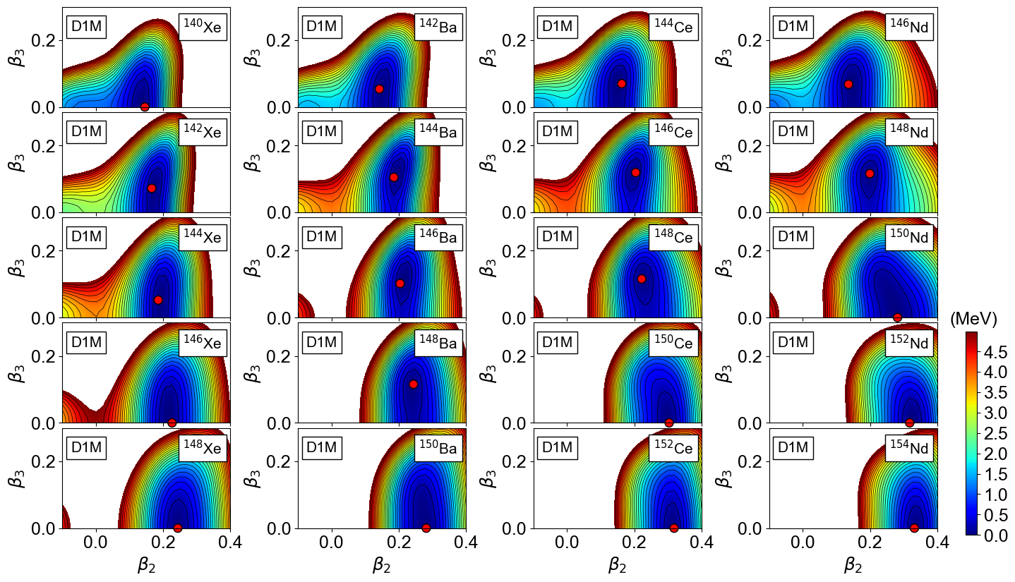
Figure 1: The SCMF-PESs obtained for ^140-148Xe, ^142-150Ba, ^144-152Ce, and ^146-154Nd are plotted as functions of the quadrupole $\beta_{2}$ and octupole $\beta_{3}$ deformation parameters. The color code indicates the total HFB energies (in MeV) plotted up to 5 MeV with respect to the global minimum. The energy difference between neighboring contours is 0.2 MeV. For each nucleus, the global minimum is indicated by a red solid circle. Results have been obtained with the Gogny-D1M EDF.

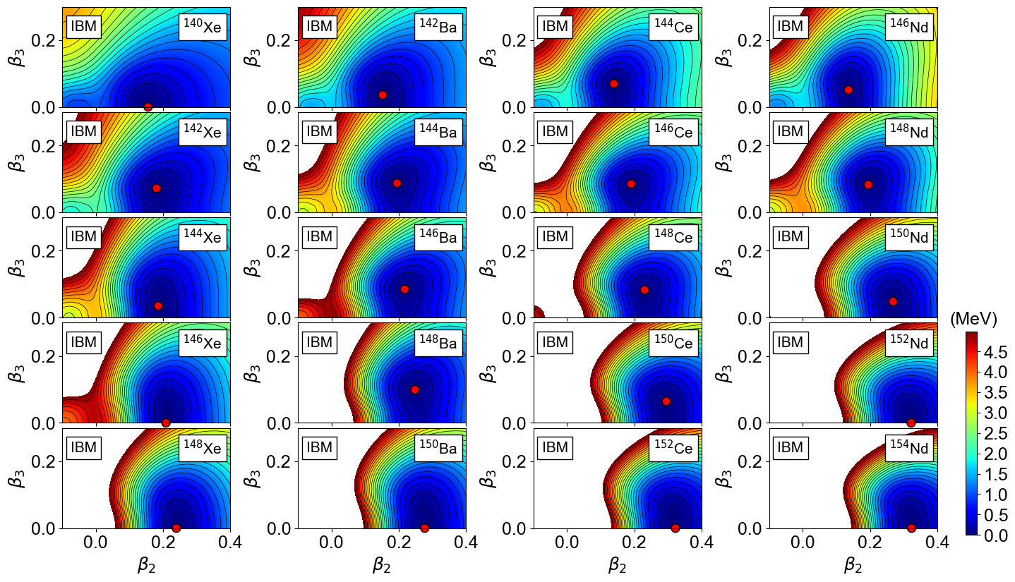
Figure 2: The same as in Fig. 1, but for the mapped IBM-PESs.

We have employed the same $sdf$-IBM Hamiltonian as in our previous studies for actinide nuclei [53, 54]:

$$\hat{H}=\epsilon_{d}\hat{n}_{d}+\epsilon_{f}\hat{n}_{f}+\kappa_{2}\hat{Q}_{2}\cdot\hat{Q}_{2}+\rho\hat{L}\cdot\hat{L}+\kappa_{3}\hat{Q}_{3}\cdot\hat{Q}_{3}.$$ (1)

The first (second) term represents the number operator for the $d$ ($f$) bosons with $\epsilon_{d}$ ($\epsilon_{f}$) being the single $d$ ($f$) boson energy relative to the $s$ boson one. The third, fourth and fifth terms represent the quadrupole-quadrupole interaction, the rotational term, and the octupole-octupole interaction, respectively. The quadrupole $\hat{Q}_{2}$, the angular momentum $\hat{L}$, and the octupole $\hat{Q}_{3}$ operators read

$$\hat{Q}_{2}=s^{\dagger}\tilde{d}+d^{\dagger}\tilde{s}+\chi_{d}(d^{\dagger}\tilde{d})^{(2)}+\chi_{f}(f^{\dagger}\tilde{f})^{(2)}$$ (2a)

$$\hat{L}=\sqrt{10}(d^{\dagger}\tilde{d})^{(1)}+\sqrt{28}(f^{\dagger}\tilde{f})^{(1)}$$ (2b)

$$\hat{Q}_{3}=s^{\dagger}\tilde{f}+f^{\dagger}\tilde{s}+\chi_{3}(d^{\dagger}\tilde{f}+f^{\dagger}\tilde{d})^{(3)}.$$ (2c)

Note that the term proportional to $(d^{\dagger}\tilde{d})^{(1)}\cdot(f^{\dagger}\tilde{f})^{(1)}$ in the $\hat{L}\cdot\hat{L}$ term has been neglected [53]. The parameters $\epsilon_{d}$, $\epsilon_{f}$, $\kappa_{2}$, $\rho$, $\chi_{d}$, $\chi_{f}$, $\kappa_{3}$, and $\chi_{3}$ of the $sdf$-IBM Hamiltonian are determined, for each nucleus, in such a way [52, 53] that the expectation value of the $sdf$-IBM Hamiltonian in the boson condensate state (denoted by IBM-PES), $E_{\mathrm{IBM}}(\beta_{2},\beta_{3})=\bra{\phi(\beta_{2},\beta_{3})}\hat{H}\ket{\phi(\beta_{2},\beta_{3})}$, reproduces the SCMF-PES $E_{\mathrm{HFB}}(\beta_{2},\beta_{3})$ in the neighborhood of the global minimum. The boson condensate state is given by [71]:

$$|\phi(\beta_{2},\beta_{3})\rangle=(n!)^{-1/2}(b_{c}^{\dagger})^{n}\ket{0}$$ (3a)

with

$$b_{c}^{\dagger}=(1+{\bar{\beta}_{2}}^{2}+{\bar{\beta}_{3}}^{2})^{-1/2}(s^{\dagger}+\bar{\beta}_{2}d_{0}^{\dagger}+\bar{\beta}_{3}f_{0}^{\dagger}),$$ (3b)

where $\ket{0}$ denotes the boson vacuum, or inert core. In the present work, the doubly-magic nucleus ¹³²Sn is taken as the inert core, hence $n=(A-132)/2$ for a nucleus with mass number $A$. The amplitudes $\bar{\beta}_{2}$ and $\bar{\beta}_{3}$ entering the definition of the boson condensate wave function are assumed to be proportional to the deformation parameters $\beta_{2}$ and $\beta_{3}$ of the fermionic space, $\bar{\beta}_{2}=C_{2}\beta_{2}$ and $\bar{\beta}_{3}=C_{3}\beta_{3}$ [71, 51, 52], with dimensionless proportionality constants $C_{2}$ and $C_{3}$. The reason for the scaling is that the present version of the IBM is built on a restricted model space of valence nucleons in one major shell, while the SCMF model is defined on the entire fermion Hilbert space. The difference between the fermionic and bosonic model spaces is effectively accounted for by the constants $C_{2}$ and $C_{3}$. Their values are also determined by the mapping procedure so that the location of the global minimum in the SCMF-PES is reproduced. The parameter $\rho$ is fixed separately [72] by equating the cranking moment of inertia obtained in the intrinsic frame of the IBM [73] at the equilibrium minimum to the corresponding Thouless-Valatin value [74] computed by the Gogny-HFB method. A more detailed description of the whole procedure can be found in Ref. [53]. The analytical form of the IBM-PES $E_{\mathrm{IBM}}(\beta_{2},\beta_{3})$ is given in Ref. [52]. For the numerical diagonalization of the mapped Hamiltonian $\hat{H}$ (1), the computer code arbmodel [75] has been used.

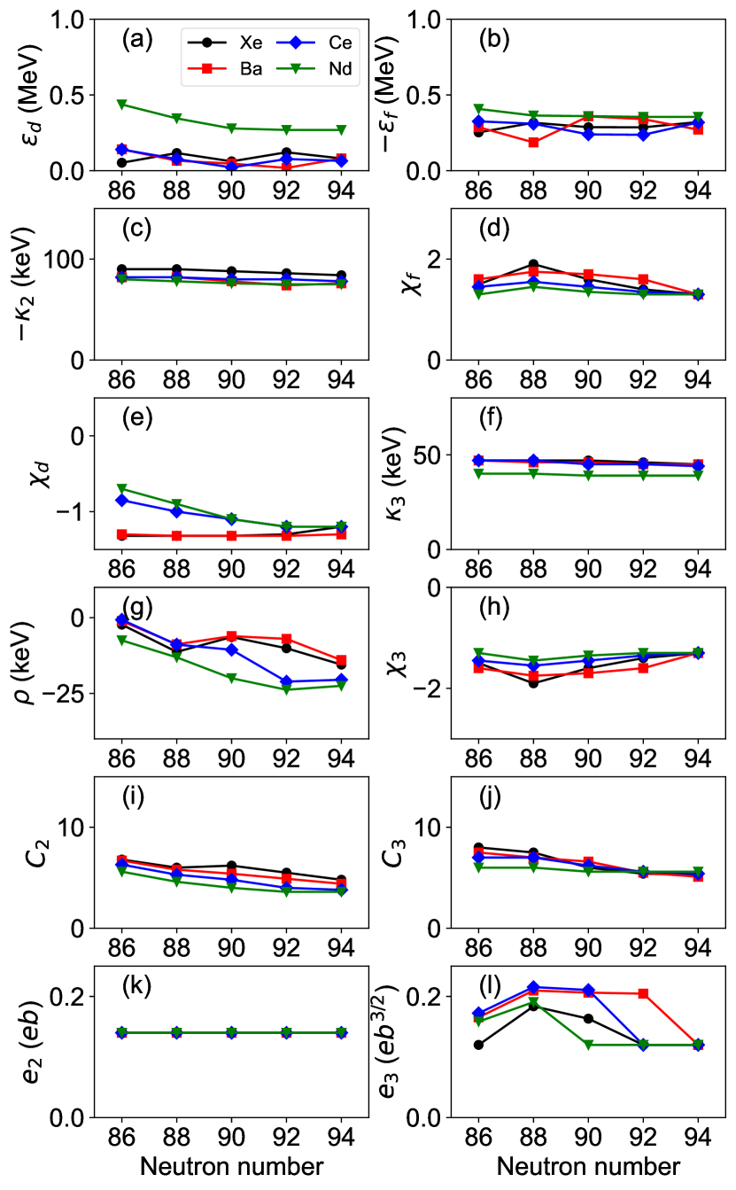
Figure 3: The strength parameters (a) $\epsilon_{d}$, (b) $\epsilon_{f}$, (c) $\kappa_{2}$, (d) $\chi_{f}$, (e) $\chi_{d}$, (f) $\kappa_{3}$, (g) $\rho$, and (h) $\chi_{3}$ of the $sdf$-IBM Hamiltonian (1), and the coefficients (i) $C_{2}$ and (j) $C_{3}$ are plotted as functions of the neutron number for the studied isotopic chains. The boson effective charges for the quadrupole $e_{2}$ and octupole $e_{3}$ transitions are also plotted in panels (k) and (l), respectively.

III Results and discussions

In this section we discuss the results of the calculations. Attention is paid to the SCMF- and IBM-PESs in Sec. III.1, the evolution of the low-energy excitation spectra in Sec. III.2, alternating-parity structures in Sec. III.3 and transition rates in Sec. III.4. The detailed spectroscopy of selected nuclei is considered in Sec. III.5.

III.1 Potential energy surfaces

The $(\beta_{2}$, $\beta_{3})$ Gogny-HFB SCMF-PESs obtained for the considered Xe, Ba, Ce, and Nd nuclei are depicted in Fig. 1. In a number of nuclei close to the neutron number $N=88$ a minimum with $\beta_{3}\approx 0.1$ is obtained. The most prominent example is the Ba chain where four of the studied isotopes exhibit a (static) octupole-deformed ground state. These SCMF results are consistent with the empirical fact that octupole correlations are enhanced near $Z=56$ and $N=88$. For heavier nuclei, the ground state is reflection symmetric while the potential is still rather soft along the $\beta_{3}$-direction. Note, that this octupole softness, characteristic of an octupole vibrational regime, indicates that octupole correlations are still important even though the global minimum of the PESs occur at $\beta_{3}=0$. On the other hand, the $\beta_{2}$ value at the minimum increases with neutron number.

In Fig. 2 we have plotted the corresponding IBM-PESs. Comparing with Fig. 1 we conclude that the essential features of the SCMF-PESs in the vicinity of the global minimum are reproduced by the IBM-PESs. However, some differences are observed: for ¹⁵⁰Ce and ¹⁵⁰Nd the IBM-PESs exhibit global minima at non-zero $\beta_{3}$ deformation, whereas the SCMF-PESs for these nuclei show reflection symmetric ($\beta_{3}=0$) minima. A closer look reveals that those discrepancies are rather insignificant and they should have little impact on the spectroscopic properties: the depth of the octupole deformed IBM-PES minima do not exceed 20 keV and the SCMF-PES are are also considerably soft along the $\beta_{3}$ direction. For lighter isotopes, the IBM-PESs are much flatter than the SCMF-PESs. This is a feature already observed in previous studies using the SCMF-to-IBM mapping procedure [53, 54]. It is another consequence of the mapped IBM being built on a restricted model (valence) space while the SCMF model considers all the nucleons.

The parameters of the mapped IBM Hamiltonian are shown in Figs. 3(a) to 3(h) while the proportionality constants $C_{\lambda}$ are depicted in Figs. 3(i) and 3(j). Most of the Hamiltonian parameters exhibit a gradual change as functions of the neutron number and their systematic trend is similar in neighboring isotopic chains. The stability of those parameters as functions of the nucleon number is particularly important and satisfying, as it reveals the robustness of the mapping procedure in the considered mass region.

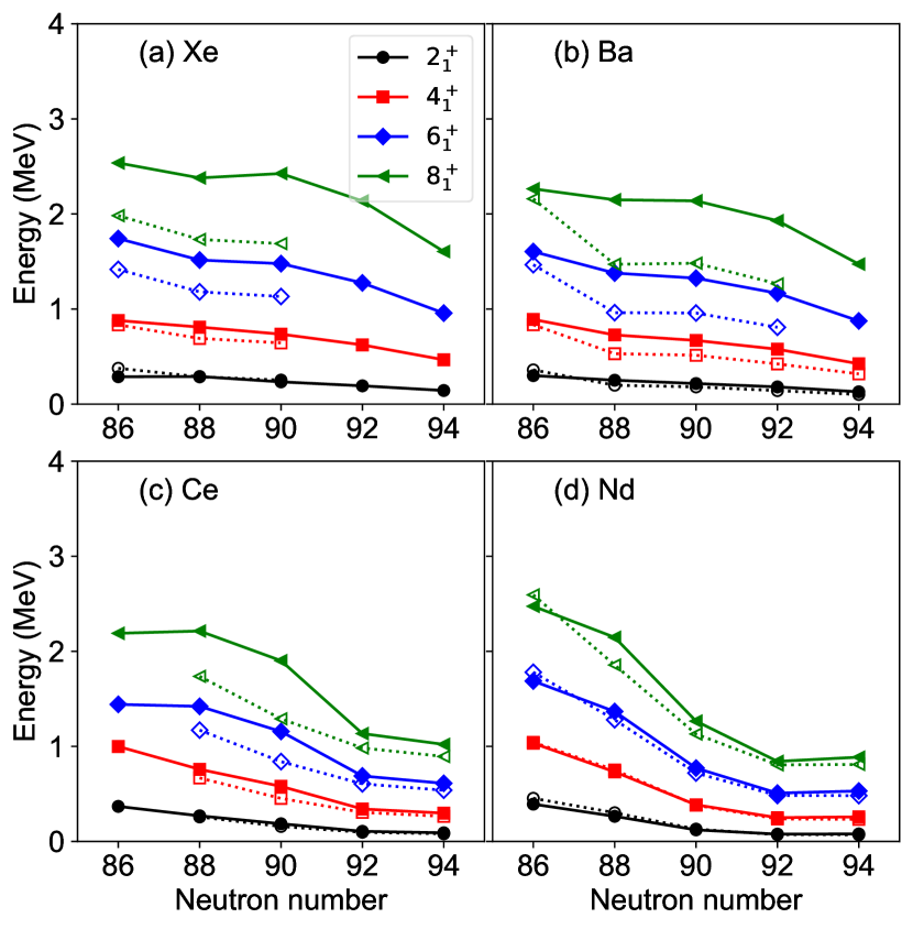
Figure 4: The low-energy excitation spectra of positive-parity even-spin yrast states in ^140-148Xe, ^142-150Ba, ^144-152Ce and ^146-154Nd, computed by diagonalizing the mapped $sdf$-IBM Hamiltonian (1), are shown as functions of the neutron number. Experimental data have been taken from Ref. [76].

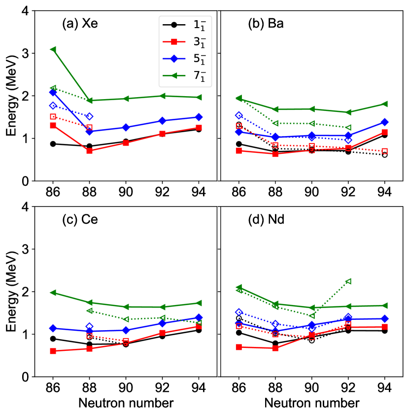
Figure 5: The same as in Fig. 4 but for odd-spin negative-parity yrast states.

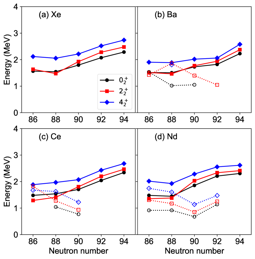
Figure 6: The same as in Fig. 4 but for the $0^{+}_{2}$, $2^{+}_{2}$, and $4^{+}_{2}$ states. The experimental data are taken from Refs. [76, 77].

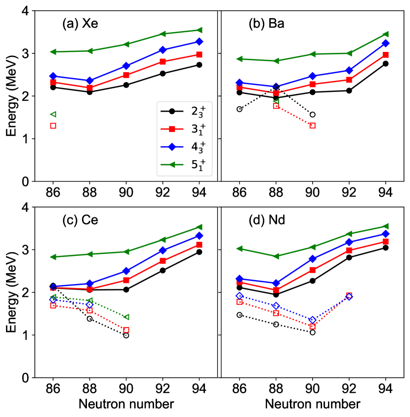
Figure 7: The same as in Fig. 4 but for the $2^{+}_{3}$, $3^{+}_{1}$, $4^{+}_{3}$, and $5^{+}_{1}$ states. The experimental data are taken from Refs. [76, 77].

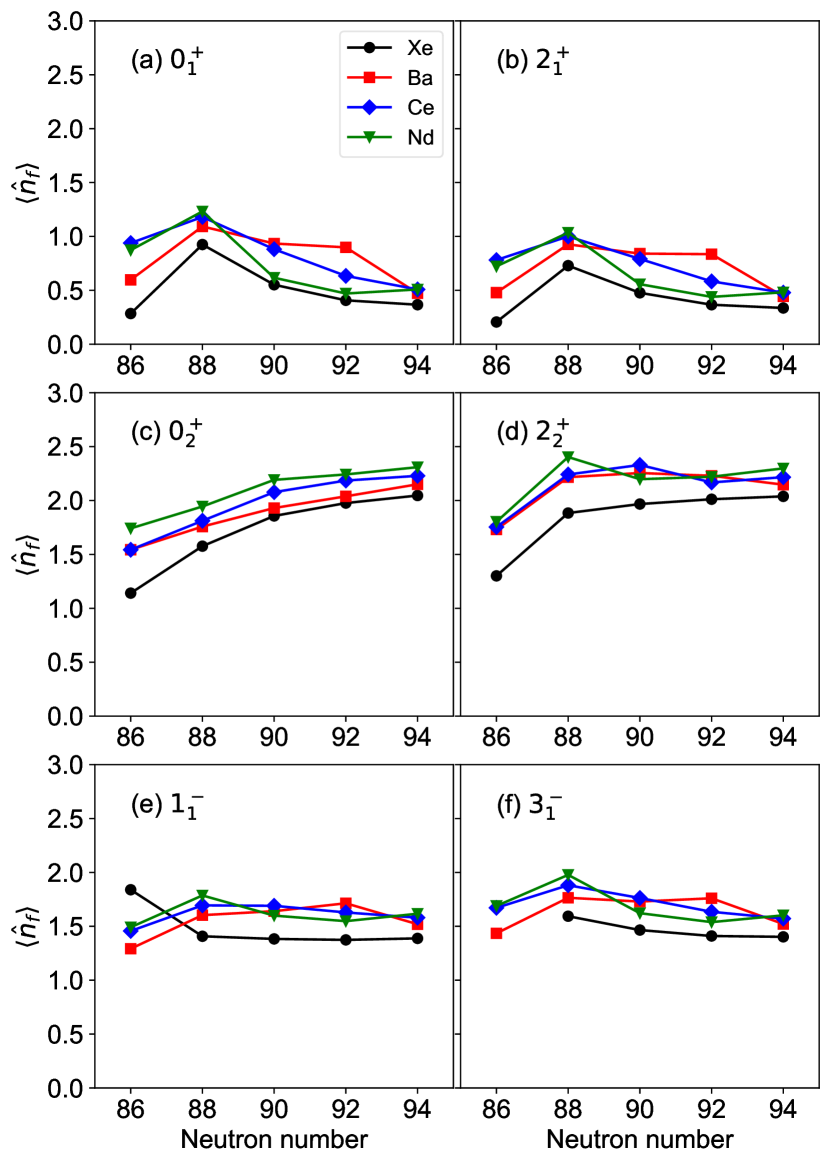
Figure 8: The expectation values of the $f$-boson number operator $\braket{\hat{n_{f}}}$ in the IBM wave functions corresponding to the states (a) $0^{+}_{1}$, (b) $2^{+}_{1}$, (c) $0^{+}_{2}$, (d) $2^{+}_{2}$, (e) $1^{-}_{1}$, and (f) $3^{-}_{1}$ are plotted as functions of the neutron number.

III.2 Evolution of low-energy excitation spectra

The excitation spectra corresponding to the positive-parity even-spin and negative-parity odd-spin yrast states obtained in our calculations for Xe, Ba, Ce, and Nd nuclei are plotted in Figs. 4 and 5, respectively. The available experimental data taken from the NNDC database [76] are shown in the same figures.

As can be seen from Fig. 4, both the theoretical and experimental positive-parity yrast states exhibit a monotonic decrease as functions of the neutron number. This is a typical feature of a near-spherical-to-deformed shape transition. The impact of the shape phase transitions in the positive-parity states in the neutron-rich Ba region were also considered in empirical studies (e.g., Refs. [78, 79, 80]). In the case of the Ce and Nd isotopes, the calculations predict a pronounced structural change between $N=90$ and 92. The positive-parity ground-state band obtained with the mapped IBM model exhibits a qualitatively similar pattern when compared with the experimental one. At the quantitative level most of the studied nuclei with $N<92$ show a considerably stretched theoretical ground-state band implying that the moment of inertia is too small as compared with the experimental one. This is probably a consequence of the too large quadrupole-quadrupole interaction strength $\kappa_{2}$ determined by the mapping procedure. The value of the derived parameter, in turn, reflects the topology of the Gogny-D1M SCMF-PES which exhibits a pronounced minimum with a non-zero octupole deformation $\beta_{3}$ (see, Fig. 1). To reproduce such a topology of the SCMF-PES in the IBM energy surface a large value of the strength parameter $\kappa_{2}$ is required. Another likely explanation is that, especially for lighter nuclei near the shell closure, the number of bosons is not large enough to describe satisfactorily the excitation energies with spin $I\geqslant 6^{+}$.

A characteristic signature of octupole collectivity is the lowering of the low-lying negative-parity states with respect to the positive-parity ground-state band. As can be seen from Fig. 5, for each of the studied isotopic chains, such a pattern is observed in both the theoretical and experimental negative-parity levels. The excitation energies of the predicted negative-parity bands decrease toward $N\approx 88$. For most of the studied isotopic chains the $3^{-}$ excitation energy reaches its minimum value around this neutron number. For $N>88$ the excitation energies of the negative-parity levels gradually increase. This reflects the fact that, at the HFB level, the octupole minimum becomes less pronounced as $N$ increases. However, the negative-parity excitation energies remain rather constant for the Ba isotopes up to $N=92$. At the HFB level, an octupole-deformed ground state is indeed found in Ba isotopes with neutron number between 86 and 92 (cf. Figs. 1 and 2). Similar results are obtained for Ce isotopes. In the case of Xe and Nd isotopes, an approximate parabolic systematic is observed in the predicted levels around $N=88$ and 90. The systematic of the negative-parity states already discussed, suggests that in the neutron-rich lanthanide region, octupole collectivity evolves moderately. This is at variance with the structural change observed in light actinides, especially Ra and Th isotopes. In that case the parabolic dependence on neutron number of the negative-parity band energy is stronger [54], with the lowest energy at $N\approx 134$. The negative-parity bands predicted for Ba and Xe isotopes are systematically stretched as compared with the experimental ones. The reason is the same as in the case of the positive-parity states in Fig. 4.

Figure 6 displays the excitation energies of the non-yrast states $0^{+}_{2}$, $2^{+}_{2}$, and $4^{+}_{2}$. For nuclei with $N\geqslant 90$ those states appear to form a quasi-$\beta$ band with the $0^{+}_{2}$ state as the bandhead. For the transitional nuclei with $N<90$, Fig. 6 shows that the computed energy levels display a more irregular pattern, with an inversion of the position of the $0^{+}_{2}$ and $2^{+}_{2}$ energy levels. In the transitional region, the SCMF-PESs are rather soft both along the $\beta_{2}$ and $\beta_{3}$ deformations, indicating considerable shape mixing. As a consequence, the level repulsion among low-spin states is so strong as to explain the irregular band structure. In addition, as one can see most noticeably in the strongly quadrupole deformed Ce and Nd isotopes in Figs. 6(c) and 6(d), respectively, the calculated energy levels are considerably higher than the experimental ones. This is a common feature in mapped IBM studies, that is mainly due to the unexpectedly large $\kappa_{2}$ value.

Figure 7 depicts the excitation spectra for another set of non-yrast states, $2^{+}_{3}$, $3^{+}_{1}$, $4^{+}_{3}$, and $5^{+}_{1}$. The present calculation suggests that in most of the considered nuclei these states are members of quasi-$\gamma$ bands. In fact, as can be seen in Fig. 7, the energy levels look more or less harmonic. Only the $5^{+}_{1}$ level, especially for lighter isotopes with $N<90$, is much higher in energy than the other members of the band. For the same reason as in the case of the quasi-$\beta$ band, the experimental bandhead energy of the quasi-$\gamma$ band is considerably overestimated.

We have plotted in Fig. 8 the expectation value of the $f$-boson number operator $\hat{n}_{f}$ obtained with the IBM wave functions of the states (a) $0^{+}_{1}$, (b) $2^{+}_{1}$, (c) $0^{+}_{2}$, (d) $2^{+}_{2}$, (e) $1^{-}_{1}$, and (f) $3^{-}_{1}$. It is remarkable that, at $N\approx 88$, both the wave functions of the $0^{+}_{1}$ and $2^{+}_{1}$ states contain a large amount of $f$-boson components $\braket{\hat{n}_{f}}\approx 1$. This suggests that the octupole degree of freedom plays an important role in the structure of the positive-parity ground-state bands at low spin for $N\approx 88$ nuclei. Exception made of the Xe isotopes, the $0^{+}_{2}$ state appears to be of double-octupole boson nature because $\braket{\hat{n}_{f}}\approx 2$. The $f$-boson content of the $2^{+}_{2}$ state is similar to that of the $0^{+}_{2}$ state, especially for $N\geqslant 88$. The number of $f$ bosons in the wave functions of the $1^{-}_{1}$ and $3^{-}_{1}$ states is in the range $1\leqslant\braket{\hat{n}_{f}}\leqslant 2$. Note that the contribution of the $f$ boson to the wave functions is particularly large $\braket{\hat{n}_{f}}\approx 2$ around $N=88$, where the SCMF-PESs exhibit the most pronounced octupole deformation effects.

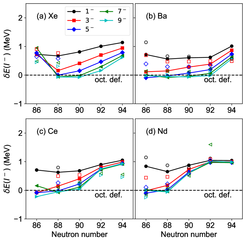
Figure 9: The energy displacement $\delta E(I^{-})$ (4) is plotted as a function of the neutron number. The theoretical values are connected by lines. Experimental values [76] for the $I^{\pi}=1^{-}$, $3^{-}$, $5^{-}$, $7^{-}$, and $9^{-}$ yrast states are represented by open circles, squares, diamonds, and left- and right-pointing triangles, respectively. A broken horizontal line in each panel stands for the limit of stable octupole deformation $\delta E(I^{-})=0$.

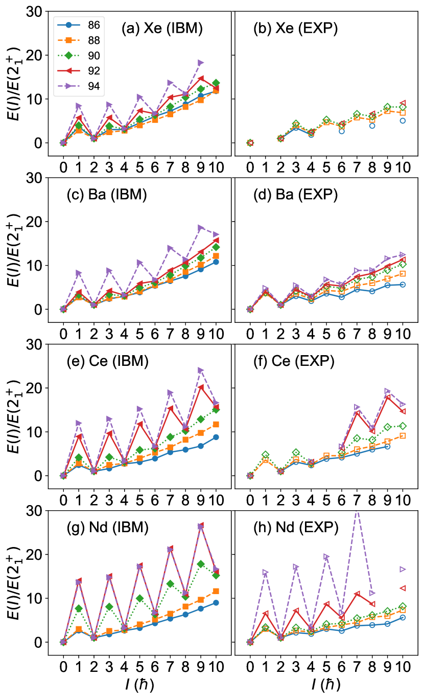
Figure 10: The energy ratio $E(I^{\pi})/E(2^{+}_{1})$ is depicted as a function of the spin $I^{\pi}$. For more details, see the main text.

III.3 Possible alternating-parity band structure

In order to distinguish whether the members of rotational bands are octupole-deformed or octupole vibrational states, it is convenient to analyze the energy displacement defined by

$$\delta E(I^{-})=E(I^{-})-\frac{E((I+1)^{+})+E((I-1)^{+})}{2},$$ (4)

where $E(I^{-})$ and $E((I\pm 1)^{+})$ represent excitation energies of the odd-spin negative-parity and even-spin positive-parity yrast states, respectively. If the positive- and negative-parity bands share an octupole deformed bandhead they form an alternating-parity doublet and the quantity $\delta E(I^{-})$ is equal to zero. The deviation from the limit $\delta E(I^{-})=0$ means that the states generating the positive- and negative-parity bands are very different, and therefore the negative parity state must be of octupole vibrational character.

The results obtained for the energy displacement Eq. (4) are displayed in Fig. 9. For almost all the studied nuclei, the energy displacement corresponding to the low-lying negative-parity states is close to the limit of stable octupole deformation $\delta E(I^{-})=0$ for $N\leqslant 90$. However, the $\delta{E}(I^{-})$ values obtained for Ce and Nd isotopes with $N>90$ depart sharply from that limit. This is in correspondence with the differences observed between the low-energy positive- and negative-parity levels in these isotopes and the ones observed in the Ba and Xe chains (cf. Figs. 4 and 5).

As yet another signature of the formation of alternating-parity doublets, we study the energy ratio $E(I^{\pi})/E(2^{+}_{1})$. For an ideal alternating-parity band, this quantity depends quadratically on the spin $I$. On the other hand, in the case of octupole vibrational states the positive- and negative-parity bands are decoupled and the ratio should also increase quadratically but with a different curvature (inverse of the moment of inertia) and therefore a staggering pattern as a function of the spin is expected. As can be seen in Fig. 10 for the Ce and Nd isotopes both the predicted and experimental energy ratios $E(I^{\pi})/E(2^{+}_{1})$ increase quadratically with spin $I$ up to $N=88-90$ while a staggering pattern emerges for larger neutron numbers. These phenomena are also observed in other mass regions, and appear to be characteristic of those nuclei where octupole correlations play an important role in low-lying states. A similar staggering pattern of the ratio $E(I^{\pi})/E(2^{+}_{1})$ appears at $N\approx 134$ in light actinide and at $N\approx 88$ in rare-earth regions in the calculations based on the relativistic Hartree-Bogoliubov mean field with the DD-PC1 EDF [51].

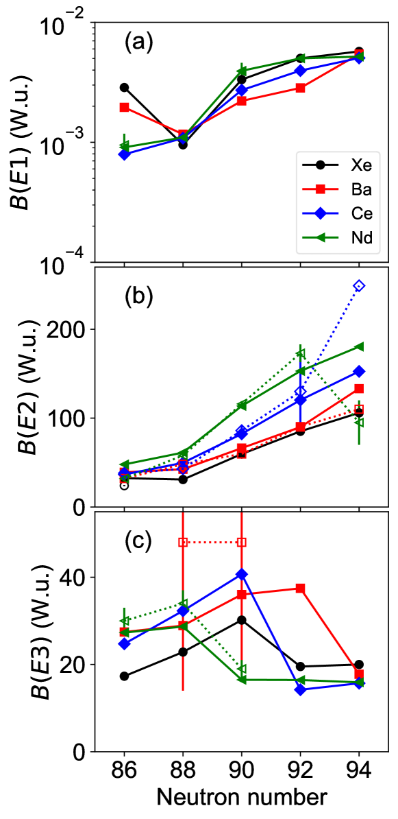
Figure 11: The $B(E1;1^{-}_{1}\to 0^{+}_{1})$ (top), $B(E2;2^{+}_{1}\to 0^{+}_{1})$ (middle), and $B(E3;3^{-}_{1}\to 0^{+}_{1})$ (bottom) reduced transition probabilities (in Weisskopf units) are compared with the experimental data [76, 5, 6, 81].

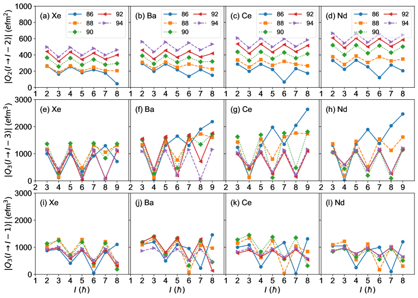
Figure 12: The theoretical quadrupole $Q_{2}(I\to I-2)$ (top), octupole $Q_{3}(I\to I-3)$ (middle), and $Q_{3}(I\to I-1)$ (bottom) moments in $e$fm^λ units are plotted as as functions of the spin $I$. Even- (Odd-) $I$ values correspond to positive- (negative-) parity states.

III.4 Transition rates

Transition probabilities are computed using the electric dipole, quadrupole, and octupole transition operators $\hat{T}(E\lambda)$ ($\lambda=1,2,3$) defined as $\hat{T}(E1)=e_{1}(d^{\dagger}\tilde{f}+f^{\dagger}\tilde{d})^{(1)}$, $\hat{T}(E2)=e_{2}\hat{Q}_{2}$, and $\hat{T}(E3)=e_{3}\hat{Q}_{3}$. The operators $\hat{Q}_{2}$ and $\hat{Q}_{3}$ are the same as those introduced in Eqs. (2a) and (2c), respectively. The boson effective charges $e_{1}=0.02$ $e$b^1/2, $e_{2}=0.14$ $e$b, are fixed so that the experimental $B(E1;1^{-}_{1}\to 0^{+}_{1})$, $B(E2;2^{+}_{1}\to 0^{+}_{1})$ transition rates are reproduced reasonably well. However, in order to fix $e_{3}$ it is needed to consider the large $B(E3;3^{-}_{1}\to 0^{+}_{1})$ values observed experimentally in those nuclei where octupole correlations are enhanced. In order to account for this fact, the effective $E3$ charge is assumed to depend on the deformation parameters as $e_{3}=0.12\times(1+\bar{\beta_{2}}\bar{\beta_{3}})$ $e$b^3/2. The $e_{2}$ and $e_{3}$ charges employed in the calculations are shown in Figs. 3(k) and 3(l) as functions of the neutron number. The behavior of the charge $e_{3}$ corresponds to an inverted parabola with a maximum around $N=88$, i.e., the neutron number for which the global minimum of the SCMF-PESs is reflection asymmetric.

The $B(E1;1^{-}_{1}\to 0^{+}_{1})$, $B(E2;2^{+}_{1}\to 0^{+}_{1})$, and $B(E3;3^{-}_{1}\to 0^{+}_{1})$ reduced transition probabilities obtained in the calculations are compared with the experimental data [76, 5, 6, 81] in Fig. 11. The $B(E1)$ and $B(E2)$ rates agree well with the experimental ones. They show a steep increase beyond $N=88-90$ that is consistent with the development of strong collectivity. Moreover, for each isotopic chain, the largest $B(E3)$ rate corresponds to $N\approx 88$. The computed $B(E3)$ values also agree reasonably well with the experimental ones. In particular, for ^144,146Ba the predicted $B(E3)$ rates are within the experimental error bars [5, 6].

We have obtained the transition quadrupole $Q_{2}(I\to I^{\prime})$ and octupole $Q_{3}(I\to I^{\prime})$ moments from the reduced $E2$ and $E3$ matrix elements resulting from the diagonalization of the $sdf$-IBM Hamiltonian. Those transition multipole moments $Q_{\lambda}(I\to I^{\prime})$ ($\lambda=2,3$) read

$$Q_{\lambda}(I\to I^{\prime})= \braket{I^{\prime}}{\hat{T}(E\lambda)}{I}$$

$$\times\sqrt{\frac{16\pi}{(2\lambda+1)(2I+1)}}(I\lambda 00|I^{\prime}0)^{-1},$$ (5)

where the factor $(I\lambda 00|I^{\prime}0)$ represents a Clebsch-Gordan coefficient.

The quadrupole $Q_{2}(I^{\pm}\to(I-2)^{\pm})$ and octupole moments $Q_{3}(I^{\pm}\to(I-3)^{\mp})$ and $Q_{3}(I^{\mp}\to(I-1)^{\pm})$ ($e$fm^λ units) are depicted in Fig. 12 as functions of the spin. The transitions between even-spin (odd-spin) positive (negative) parity states are used to compute the quadrupole moment $Q_{2}$ while the octupole moments, involve $E3$ transitions between even-spin positive-parity and odd-spin negative-parity states.

The $Q_{2}$ moments in each of the in-band $I^{\pm}\to(I-2)^{\pm}$ transitions are depicted in the top row of Fig. 12 as functions of the spin. They exhibit a slight odd-even spin staggering pattern. Exception are the $Q_{2}$ moments for the lightest $N=86$ isotopes, where a certain irregularity arises for the spin $I\geqslant 6$ because of the change in the structure of the wave function around $I=6^{+}$. For example, in the case of ¹⁴⁴Ce, the states in the ground-state band mainly consist of monopole $s$ and quadrupole $d$ bosons up to $I=4^{+}$. However, for larger spin values the $f$ boson degree of freedom plays a role since $\braket{\hat{n}_{f}}\approx 2$. This leads to the small $\braket{4^{+}}{\hat{T}(E2)}{6^{+}}$ matrix element. In addition, at a given spin $I$, the $Q_{2}$ value increases as a function of the neutron number, reflecting the increasing quadrupole collectivity as the number of valence nucleons increases.

The $Q_{3}(I\to I-3)$ moments are plotted in the middle row of Fig. 12 as functions of the spin. They exhibit a staggering pattern. In most of the studied isotopic chains, the calculated $Q_{3}(I^{+}\to(I-3)^{-})$ moments nearly vanish for even spin $I$. Here, one should keep in mind that the measured reduced $E3$ matrix elements between the states $I^{+}$ and $(I-3)^{-}$ (with $I$ even) in ^148,150Nd [82, 83] are close to zero. Furthermore, the values in the range $1000-2000$ $e$fm³ obtained for $Q_{3}(I^{-}\to(I-3)^{+})$ (with $I$ odd) are consistent with the experimental data [3].

A similar staggering pattern is observed for $Q_{3}(I\to I-1)$, plotted in the bottom row of Fig. 12 as functions of the spin. In good agreement with the empirical trend in this mass region [2, 3], the $Q_{3}(I^{+}\to(I-1)^{-})$ moments (with $I$ even) for ¹⁴⁸Nd decreases with the spin. The $Q_{3}(I^{-}\to(I-1)^{+})$ moments (with $I$ odd) for the same nucleus are calculated to be $\approx 1000$ $e$fm³, while experimentally the corresponding values are close to zero.

Figure 13: Comparison of the theoretical and experimental low-energy level schemes of (a) ¹⁴⁴Ba, (b) ¹⁴⁸Nd, and (c) ¹⁵⁰Nd. The experimental data have been taken from Ref. [76].

Table 1: The $B(E1)$, $B(E2)$, and $B(E3)$ transition rates (in Weisskopf units) obtained for ¹⁴⁴Ba and ¹⁴⁶Ba are compared with the experimental data [5, 6].

	$E\lambda$	$I_{i}$	$I_{f}$	EXP	IBM
144Ba	$E2$	$2^{+}_{1}$	$0^{+}_{1}$	48${}^{+2}_{-2}$	43
		$4^{+}_{1}$	$2^{+}_{1}$	86${}^{+10}_{-7}$	61
		$6^{+}_{1}$	$4^{+}_{1}$	54${}^{+7}_{-6}$	57
		$8^{+}_{1}$	$6^{+}_{1}$	55${}^{+19}_{-12}$	37
	$E3$	$3^{-}_{1}$	$0^{+}_{1}$	48${}^{+25}_{-34}$	29
		$5^{-}_{1}$	$2^{+}_{1}$	$<103$	50
		$7^{-}_{1}$	$4^{+}_{1}$	$<135$	63
146Ba	$E1$	$1^{-}_{1}$	$0^{+}_{1}$	9.3${}^{+0.8}_{-0.7}\times 10^{-7}$	2.2$\times 10^{-3}$
			$2^{+}_{1}$	$(6.6\pm 0.5)\times 10^{-6}$	3.3$\times 10^{-5}$
		$3^{-}_{1}$	$4^{+}_{1}$	$(1.59\pm 0.09)\times 10^{-5}$	8.4$\times 10^{-3}$
			$2^{+}_{1}$	$(1.84\pm 0.13)\times 10^{-6}$	2.7$\times 10^{-4}$
	$E2$	$2^{+}_{1}$	$0^{+}_{1}$	60$\pm 2$	66
		$4^{+}_{1}$	$2^{+}_{1}$	94$\pm 24$	93
		$6^{+}_{1}$	$4^{+}_{1}$	93${}^{+23}_{-27}$	94
		$8^{+}_{1}$	$6^{+}_{1}$	61${}^{+48}_{-24}$	73
		$3^{-}_{1}$	$1^{-}_{1}$	45$\pm 38$	50
	$E3$	$3^{-}_{1}$	$0^{+}_{1}$	48${}^{+25}_{-29}$	36
		$5^{-}_{1}$	$2^{+}_{1}$	73${}^{+88}_{-29}$	60
		$7^{-}_{1}$	$4^{+}_{1}$	82${}^{+112}_{-45}$	73
		$9^{-}_{1}$	$6^{+}_{1}$	94${}^{+100}_{-94}$	39

Table 2: Same as in Table 1, but for ¹⁴⁸Nd and ¹⁵⁰Nd. Experimental data have been taken from Ref. [76].

	$E\lambda$	$I_{i}$	$I_{f}$	EXP	IBM
148Nd	$E1$	$5^{-}_{1}$	$4^{+}_{1}$	0.00205$\pm 0.00021$	0.014
		$7^{-}_{1}$	$6^{+}_{1}$	0.0043$\pm 0.0010$	0.020
		$8^{+}_{1}$	$7^{-}_{1}$	0.0049$\pm 0.0011$	0.0094
	$E2$	$2^{+}_{1}$	$0^{+}_{1}$	57.9$\pm 2.2$	61
		$4^{+}_{1}$	$2^{+}_{1}$	94$\pm 4$	92
		$0^{+}_{2}$	$2^{+}_{1}$	31.2$\pm 2.2$	52
		$2^{+}_{2}$	$0^{+}_{1}$	0.54$\pm 0.08$	2.6
			$2^{+}_{1}$	14.4$\pm 1.9$	6.0
			$4^{+}_{1}$	16$\pm 8$	4.4
		$2^{+}_{3}$	$0^{+}_{1}$	1.9$\pm 0.4$	2.6
		$6^{+}_{1}$	$4^{+}_{1}$	102$\pm 7$	96
		$8^{+}_{1}$	$6^{+}_{1}$	98$\pm 17$	86
		$7^{-}_{1}$	$5^{-}_{1}$	$(1.5\pm 0.6)\times 10^{2}$	74
	$E3$	$3^{-}_{1}$	$0^{+}_{1}$	34$\pm 3$	29
150Nd	$E1$	$1^{-}_{1}$	$0^{+}_{1}$	$3.9^{+0.6}_{-0.7}\times 10^{-3}$	$3.9\times 10^{-3}$
			$2^{+}_{1}$	$7.4^{+0.6}_{-0.7}\times 10^{-3}$	$9.7\times 10^{-4}$
		$3^{-}_{1}$	$2^{+}_{1}$	$4.2^{+0.6}_{-0.7}\times 10^{-3}$	$1.1\times 10^{-2}$
			$4^{+}_{1}$	$4.5^{+0.6}_{-0.7}\times 10^{-3}$	$1.0\times 10^{-4}$
		$5^{-}_{1}$	$4^{+}_{1}$	$7^{+9}_{-5}\times 10^{-3}$	$1.8\times 10^{-2}$
			$6^{+}_{1}$	$7^{+9}_{-5}\times 10^{-3}$	$3.2\times 10^{-7}$
		$2^{-}_{1}$	$2^{+}_{2}$	$4.9^{+2.4}_{-2.0}\times 10^{-5}$	$1.3\times 10^{-2}$
			$2^{+}_{3}$	$(6\pm 3)\times 10^{-3}$	3.5$\times 10^{-4}$
			$3^{+}_{1}$	$3.1^{+1.5}_{-1.2}\times 10^{-3}$	$1.1\times 10^{-2}$
		$3^{-}_{2}$	$2^{+}_{1}$	8.0${}^{+2.0}_{-1.9}\times 10^{-5}$	$1.0\times 10^{-4}$
			$2^{+}_{2}$	8.1${}^{+2.0}_{-1.9}\times 10^{-5}$	$1.4\times 10^{-3}$
			$2^{+}_{3}$	$(2.0\pm 0.5)\times 10^{-3}$	7.6$\times 10^{-6}$
			$3^{+}_{1}$	$2.6^{+0.7}_{-0.6}\times 10^{-3}$	6.4$\times 10^{-5}$
			$4^{+}_{1}$	$(1.7\pm 0.4)\times 10^{-4}$	$1.1\times 10^{-3}$
			$4^{+}_{2}$	$(3.7\pm 0.9)\times 10^{-4}$	$6.5\times 10^{-3}$
		$7^{-}_{1}$	$6^{+}_{1}$	$(4.3\pm 1.0)\times 10^{-3}$	$2.6\times 10^{-2}$
		$8^{+}_{1}$	$7^{-}_{1}$	$(4.9\pm 1.1)\times 10^{-3}$	1.8$\times 10^{-5}$
	$E2$	$2^{+}_{1}$	$0^{+}_{1}$	116$\pm 3$	113
		$4^{+}_{1}$	$2^{+}_{1}$	180.7$\pm 1.6$	162
		$0^{+}_{2}$	$2^{+}_{1}$	43.1$\pm 2.3$	26
		$2^{+}_{2}$	$0^{+}_{1}$	0.7$\pm 0.5$	3.1
			$0^{+}_{2}$	$(1.6\pm 1.3)\times 10^{2}$	42
			$2^{+}_{1}$	10$\pm 3$	4.8
			$4^{+}_{1}$	19$\pm 7$	11
		$2^{+}_{3}$	$0^{+}_{1}$	3.0$\pm 0.6$	0.11
			$2^{+}_{1}$	$>2.9$	0.47
			$4^{+}_{1}$	1.7$\pm 1.2$	1.9
		$6^{+}_{1}$	$4^{+}_{1}$	206$\pm 9$	175
		$8^{+}_{1}$	$6^{+}_{1}$	216$\pm 23$	175
		$4^{+}_{2}$	$2^{+}_{1}$	0.015$\pm 0.004$	3.3
			$2^{+}_{2}$	23$\pm 8$	59
			$6^{+}_{1}$	9.2$\pm 2.2$	6.5
		$4^{+}_{3}$	$2^{+}_{1}$	0.58$\pm 0.20$	0.00017
			$2^{+}_{3}$	$(1.3\pm 0.5)\times 10^{2}$	31
		$10^{+}_{1}$	$8^{+}_{1}$	201$\pm 11$	165
	$E3$	$3^{-}_{1}$	$0^{+}_{1}$	19$\pm 2$	16

III.5 Detailed level schemes

For some of the considered neutron-rich lanthanide nuclei, a wealth of experimental data is available regarding the band structure as well as the electromagnetic transition rates. In this study, we have examined in detail the low-energy spectra of ¹⁴⁴Ba, ¹⁴⁸Nd, and ¹⁵⁰Nd. The first two of them correspond to $N=88$, for which a reflection asymmetric HFB minimum has been obtained. On the other hand, ¹⁵⁰Nd exhibits a (reflection symmetric) quadrupole deformed ground state with $\beta_{2}\approx 0.3$. The theoretical bands presented in what follows have been arranged according to the dominant in-band $E2$ transitions.

Figure 13(a) shows the low-energy positive-parity bands and the negative-parity band built on the $1^{-}_{1}$ state of ¹⁴⁴Ba. The experimental data for the non-yrast positive-parity bands built on the $4^{+}$ and $3^{+}$ states are also available [77], and the corresponding theoretical bands are shown in the figure. For the yrast bands with both parities, the excitation energies obtained for $I\leqslant 5$ agree reasonably well with the experimental data of Ref.  [5]. However, both bands are somewhat stretched for higher spin as compared to the experimental ones. Note, that the inversion of the theoretical $1^{-}$ and $3^{-}$ levels might indicate that a dipole boson should be included in the calculations, in order to lower the $1^{-}$ level. The theoretical non-yrast positive-parity bands are much more stretched than the observed ones, even though the energies of the bandhead are reproduced rather well. As discussed earlier, especially for the transitional nuclei around $N=88$, due to the substantial degree of configuration mixing the repulsion between the low-spin states is so strong as to make the description of the band structure difficult particularly for non-yrast states. Another potential explanation is the large number of $f$ bosons present in the wave functions of the non-yrast states, consequence of the large number of them present in our calculation.

Experimentally, the nucleus ¹⁴⁶Ba also exhibits a stable octupole deformation [6]. The level scheme obtained for ¹⁴⁶Ba is strikingly similar to that of ¹⁴⁴Ba. As can be seen from Table 1, the $B(E1)$, $B(E2)$, and $B(E3)$ reduced transition probabilities obtained for ^144,146Ba, compare well with the experimental values [76, 5, 6]. Only the $B(E1)$ rates of ¹⁴⁶Ba differ by several orders of magnitude from the experimental ones [76]. One should, however, keep in mind that the $E1$ properties are mostly determined by non-collective single particle degrees of freedom. As the $sdf$-IBM model is built on collective nucleon pairs it is not expected to provide reliable predictions on $E1$ transition properties.

The low-energy bands obtained for the isotopes ¹⁴⁸Nd and ¹⁵⁰Nd are depicted in Figs. 13(b) and 13(c), respectively. Empirically, the ¹⁴⁸Nd nucleus is also considered [78] a transitional nucleus close to the X(5) critical point symmetry [84]. For ¹⁴⁸Nd, the agreement with the experiment is better than for ¹⁴⁴Ba. This is because the number of bosons for the former is large enough so as to provide a better quantitative description of the excitation spectra. The $1^{-}$, $3^{-}$, and $5^{-}$ energy levels are somewhat lower than the experimental ones. This correlates well with the especially pronounced reflection asymmetric minimum observed in the Gogny-D1M SCMF-PES (cf. Fig. 1).

Experimental data for $\beta$ and $\gamma$ bands, built on the $0^{+}_{2}$ and $2^{+}_{2}$ states, respectively, are available for ¹⁴⁸Nd. As can be seen from Fig. 13(b), the predicted excitation energies of both bands look somewhat irregular as compared to the experimental ones. This discrepancy can be attributed to a too strong configuration mixing between the low-spin members of these bands. The excitation energies corresponding to the even-$I$ members of the $\gamma$-band agree reasonably well with the experimental values. However, this is not the case for the odd-$I$ members where the obtained excitation energies are too high. To improve the description of the non-yrast band within the (mapped) IBM calculation, certain extensions of the model would be needed. For instance, the inclusion of a specific three-body boson interaction in the IBM Hamiltonian lowers the energies of odd-$I$ members of the $\gamma$ band [85]

As can be seen in Fig. 13(c), the lowest positive- and negative-parity bands of ¹⁵⁰Nd are reasonably well described within the mapped IBM calculations. This nucleus was considered in Ref. [80] to be close to the SU(3) limit of the IBM. In fact, several features characteristic of the SU(3) dynamical symmetry can be observed: the SCMF-PES exhibits a large quadrupole (prolate) deformation in comparison with the neighboring nucleus ¹⁴⁸Nd; the resultant yrast bands for each parity are much more compressed and resemble rotational bands (Fig. 4(d)); the moments of inertia of the positive-parity ground-state, quasi-$\beta$, and quasi-$\gamma$ bands are approximately equal to each other. On the other hand, the energies of the $\beta$ and $\gamma$ bandheads are considerably overestimated although the energy splittings between the members of the bands are well reproduced. The SCMF-to-IBM mapping procedure often yields $0^{+}_{2}$ excitation energies somewhat higher than the empirical ones. As already pointed out, this mainly comes from the large strength parameter $\kappa_{2}$ of the quadruple-quadrupole interaction. In some particular deformed nuclei, the SCMF-PES suggests a too steep valley around the minimum. To reproduce such a topology with the IBM-PES, a large quadrupole-quadrupole boson interaction strength is often required. To improve the description of the non-yrast states, specifically the excitation energies of the excited $0^{+}$ states, some other building blocks may need to be included in the mapped $sdf$-IBM framework. For instance, the dynamical pairing degree of freedom has been introduced in the mapped IBM framework [86, 87] as additional collective coordinate, and have been shown to play a crucial role in lowering the $0^{+}_{2}$ energy levels.

The mapping procedure is also able to provide the energies corresponding to non-yrast negative-parity bands. For example, in the case of ¹⁵⁰Nd the excitation energies obtained for the $3^{-}_{2}$ and $2^{-}_{1}$ states are 2.004 keV and 1678 keV which should be compared to the experimental values of 1484 keV and 1435 keV, respectively.

Finally, the $B(E1)$, $B(E2)$, and $B(E3)$ transition rates are compared with the available experimental data [76] in Table 2. Exception made of some of the $E1$ rates, the overall agreement with the experimental values is reasonable. As discussed above, the $E1$ strength has a strong dependence on non-collective single particle degrees of freedom that is impossible to reproduce within the IBM scheme.

IV Summary

In this paper, we have examined the onset of octupole deformation and the related spectroscopic properties in neutron-rich lanthanide nuclei with neutron numbers $86\leqslant N\leqslant 94$ using a mapped IBM Hamiltonian obtained from microscopic $(\beta_{2},\beta_{3})$-constrained HFB calculations based on the Gogny-D1M parametrization. At the mean-field level pronounced reflection asymmetric global minima emerge around $N=88$. For larger neutron numbers reflection symmetric ground states are obtained and the corresponding quadrupole deformations increase with neutron number.

Spectroscopic properties have been studied via the diagonalization of the $sdf$-IBM Hamiltonian, with the strength parameters obtained by mapping the SCMF-PES onto the expectation value of the Hamiltonian in the boson condensate state. The patterns exhibited by the predicted low-energy negative-parity spectra and $B(E3;3^{-}_{1}\to 0^{+}_{1})$ transition rates point towards enhanced octupolarity (Fig. 5) in $N\approx 88$ isotopes. In particular, the results obtained for the energy displacement $\delta E(I)$ (Fig. 9) and ratio $E(I)/E(2^{+}_{1})$ (Fig. 10) indicate the occurrence of an approximate alternating-parity doublet structure around $N=88$. For $N\geqslant 90$ separate positive and negative bands are obtained and an octupole vibrational regime characteristic of a $\beta_{3}$-soft potential develops.

The results obtained in this work for neutron-rich lanthanide and the ones already obtained for rare-earth [52] and light actinide [53, 54] nuclei indicate that the octupole degree of freedom plays an important role to describe the structural evolution and spectroscopic properties of the low-lying states in certain regions of the nuclear chart. In particular, the employed Gogny-EDF-based $sdf$-IBM framework provides a reasonable description of key spectroscopic properties that help to identify the interplay between the quadrupole and octupole degrees of freedom in the lanthanide region. The results of the present analysis encourage us to explore the relevance of octupole deformations in other mass regions. Within this context, proton-rich nuclei with $Z\approx N\approx 56$ appear as plausible candidates to be considered in future work. Work along these lines is in progress and will be reported in a forthcoming article.

On the other hand, disagreements between the mapped IBM results and spectroscopic data indicate needs for assessing the quality of the mapping, that is, whether the problems lie on the fermionic calculations or the mapped boson Hamiltonian. There are several prescriptions along this direction: (i) For Xe and Ba isotopes, the calculation overestimated the $6^{+}_{1}$ and $8^{+}_{1}$ excitation energies (see Fig. 4). In this region, neutrons (protons) occupy $f_{7/2}$ ($g_{7/2}$) orbitals, giving rise to the $J=6^{+}$ nucleon pairs. The inclusion of the corresponding $i$ boson in the IBM may lower the energies of those yrast states with $I\geqslant 6^{+}$. (ii) As seen from Fig. 5, the mapped IBM was not able to reproduce in detail the systematic of the $7^{-}$ energy in Ba and Nd isotopes. It would be worthwhile to see if the fermionic calculation within the GCM can reproduce the empirical tendency of this state. (iii) The calculated quasi-$\beta$ (Fig. 6) and quasi-$\gamma$ bands (Fig. 6) turned out to be considerably higher than the experimental ones. As we discussed in Sec. III.2, this is partly due to the too strong quadrupole-quadrupole interaction strength. In the deformed region, it is also well known that hexadecapole ($g$) boson plays an important role. It would be then interesting to reveal whether the inclusion of the $g$ bosons in the mapping procedure, either explicitly or by using the renormalization method of Ref. [88], can improve the description of the non-yrast states. (iv) The conventional mapping procedure within the generalized seniority scheme of the nuclear shell model [69, 70] has been successful for those nuclei near the closed shells. The results obtained from such a method for nearly spherical and vibrational nuclei could be compared with those from the SCMF-to-IBM mapping procedure.