Can we measure the collapse time of a post-merger remnant for a future GW170817-like event?

Abstract

Measuring the collapse time of a binary neutron star merger remnant can inform the physics of extreme matter and improve modelling of short gamma-ray bursts and associated kilonova. The lifetime of the post-merger remnant directly impacts the mechanisms available for the jet launch of short gamma-ray bursts. We develop and test a method to measure the collapse time of post-merger remnants. We show that for a GW170817-like event at $\sim\!40$ Mpc, a network of Einstein Telescope with Cosmic Explorer is required to detect collapse times of $\sim\!10$ ms. For a two-detector network at A+ design sensitivity, post-merger remnants with collapse times of $\sim\!10\,\mathrm{ms}$ must be $\lesssim 10$ Mpc to be measureable. This increases to $\sim\!18\Hyphdash*26$ Mpc if we include the proposed Neutron star Extreme Matter Observatory (NEMO), increasing the effective volume by a factor of $\sim\!30$.

I Introduction

Measuring the lifetimes of binary neutron star post-merger remnants can help probe extreme matter at high temperature and densities and narrow down the physics of short gamma-ray bursts (e.g., Zhang, 2019; Ciolfi, 2020). These remnants may promptly collapse into a black hole or form a hot, differentially-rotating neutron star. If the total mass of a remnant is between 1.2 and 1.5 times the maximum non-rotating neutron star mass (the Tolman-Oppenheimer-Volkov mass), then the remnant is known as a hypermassive neutron star Tolman (1939); Oppenheimer and Volkoff (1939); Breu and Rezzolla (2016); Weih et al. (2018); Baumgarte et al. (2000), which is expected to collapse to form a black hole in a timescale from milliseconds to seconds Paschalidis et al. (2012). For smaller masses, the differentially-rotating remnant will evolve into rigidly-rotating neutron star after the differential rotation is quenched. The rigidly-rotating remnant will either collapse to a black hole, or form a stable neutron star, depending on the remnant mass. See Ref. Sarin and Lasky (2020) for a recent review on the evolution of neutron star merger remnants.

Determining the collapse times of hypermassive remnants can help narrow down the nature of the central engine for short gamma-ray-bursts. Multi-messenger observations of binary neutron star merger GW170817 suggest that the remnant may have either collapsed to a black hole (e.g., Metzger et al., 2018; Gill et al., 2019; Murguia-Berthier et al., 2020), or formed a long-lived remnant (e.g. Yu et al., 2018). Measuring the collapse time of a remnant may help determine the characteristic timescales associated with short gamma-ray-bursts, aiding the selection of the central engine (for a review see Zhang (2019)). Furthermore, measuring the collapse time of the post-merger remnant may help constrain the quenching mechanism and physics of the differential rotation, which may reveal indicators towards the relative contribution of radiative (gravitational waves and neutrino) and dissipative (viscous, resistive and magnetic braking) processes within the remnant.

The direct detection of gravitational waves from future neutron star merger remnants presents a great opportunity to constrain the collapse time. Numerical-relativity simulations of merger remnants show gravitational waves predominantly emitted from the fundamental f-mode oscillation of the remnant Zhuge et al. (1994); Stergioulas et al. (2011). Gravitational waves emitted from this mode occur at $\sim\!1.8\Hyphdash*4$ kHz Takami et al. (2015); Bernuzzi et al. (2015). No post-merger remnant was detected for GW170817 by the LIGO and Virgo collaboration due to lack of sensitivity of the detectors at these frequencies. However, increased sensitivity of gravitational-wave instruments and targeted high-frequency detectors may enable future detections of post-merger remnants (e.g., Martynov et al., 2019; Ackley et al., 2020).

In this paper, we assess how well future networks of gravitational-wave detectors can measure the collapse time of a post-merger remnant. We extend a waveform model developed in Ref. Easter et al. (2020) which was derived from Refs. Bauswein et al. (2016); Bose et al. (2018), to allow the measurement of the collapse time of the post-merger remnant. Using Bayesian inference, we inject numerical-relativity gravitational waveforms that are forced to collapse into different interferometer configurations to measure the maximum distance at which we can recover the collapse time.

This paper is laid out as follows. In Section II we outline the extended waveform model along with the method of gravitational-wave injections. The results are outlined in Section III and their implications in Section IV.

II methodology

We use numerical-relativity waveforms with two different equations of state that we inject into Gaussian noise realisations determined by the gravitational-wave interferometer configuration. We modify the numerical-relativity waveforms to collapse at a given collapse time. We then use an analytic model to perform detection and parameter estimation to determine distributions of the model parameters. This model, based on two models in Refs. Bauswein et al. (2016); Bose et al. (2018), is outlined in Ref. Easter et al. (2020). See also Refs. Tsang et al. (2019); Breschi et al. (2019) for alternative models of the post-merger gravitational-wave strain.

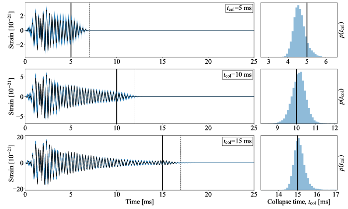
Figure 1: Time domain posterior waveforms for SLy equation of state with equal mass 1.35M_⊙ progenitor (left panels) and measured collapse times (right panels) for injections with collapse times $t_{\mathrm{col}}=5$ ms (top), $t_{\mathrm{col}}=10$ ms (centre), and $t_{\mathrm{col}}=15$ ms (bottom) injected into 2A+ detector network. Left panels show the numerical-relativity injections that have been forced to collapse (black curves) with the posterior waveforms (shaded blue curves). The right panels show the collapse-time posterior distributions for each numerical-relativity injection. The solid vertical lines on all panels shows $t_{\mathrm{col}}$ for the injected waveform. The dashed vertical lines shows $t_{\mathrm{col}}+t_{\mathrm{w}}$ where the injected signal drops to zero due to the induced collapse. Here we show three loud injections from our injection study where $t_{\mathrm{col}}$ are clearly recovered. The injected distances are 5.93 Mpc, 3.04 Mpc, and 1.00 Mpc, for 5 ms, 10 ms, and 15 ms respectively. The full posteriors for the $t_{\mathrm{col}}=10\,$ms collapse time injection are shown in the appendix (Fig B.1).

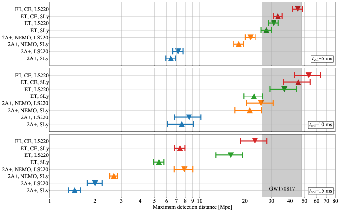
Figure 2: Maximum distances for which the collapse time can be measured for different interferometer networks and equations of state. The vertical axis shows different equations of state and interferometer configurations, and the maximum detection distance is shown on the horizontal axis. The numerical-relativity simulations are injected with equations of state SLy (upward pointing triangle) and LS220 (downward pointing triangle). The interferometer configurations are 2A+ (blue), 2A+ with the proposed Neutron star Extreme Matter Observatory (orange), Einstein Telescope (green), and Einstein Telescope with Cosmic Explorer (red). The top panel shows collapse times of 5 ms, the centre panel 10 ms and the lower panel 15 ms collapse times. The luminosity distance for GW170817 (gravitational-wave only) is shown in shaded grey for comparison Abbott et al. (2017a).

The gravitational waves from the post-merger remnant are modelled as a third-order, exponentially-damped sinusoid with a linear frequency-drift term. The plus polarisation of the gravitational-wave strain, $h_{+}(\bm{\theta},t)$, is given by:

$$h_{+}(\bm{\theta},t) =\sum_{j}h_{j,+}(\bm{\theta},t),$$

$$h_{j,+}(\bm{\theta},t) =Hw_{j}\exp\left[-\frac{t}{T_{j}}\right]\cos\left(2\pi f_{j}t\left[1+\alpha_{j}t\right]+\psi_{j}\right),$$

$$\bm{\theta} =\{H,w_{j},T_{j},f_{j},\alpha_{j},\psi_{j}:j\in[0,2]\},$$ (1)

where $\bm{\theta}$ are the model parameters and $\sum_{j}w_{j}=1$. Here, $H$ is an overall amplitude scaling factor, $w_{j}$ is the relative amplitude of the $j$th mode, $T_{j}$ is the corresponding exponential damping time constant, and $f_{j}$ is the corresponding frequency. The linear frequency-drift term is $\alpha_{j}$ and the initial phase is $\psi_{j}$. The time, $t$, is defined, such that $\max\left[h_{+}^{2}(\bm{\theta},t)+h_{\times}^{2}(\bm{\theta},t)\right]$ occurs when $t=0$. The cross polarisation for Eq. 1 is found by applying a $\pi/2$ phase shift to $\psi_{j}$. More details on this model can be found in Ref. Easter et al. (2020).

We extend this model by introducing a collapse in the gravitational-wave strain using the falling edge of a Tukey window. The falling edge starts at the collapse time, $t_{\mathrm{col}}$, and by the time $t=t_{\mathrm{col}}+t_{\mathrm{w}}$ the gravitational-wave strain drops to zero (see Fig. 1). Here $t_{\mathrm{w}}$ is the time taken for the gravitational-wave signal to completely decay. We have chosen $t_{\mathrm{w}}=2$ ms from examining numerical-relativity simulations with collapsing remnants (e.g., simulation labels: BAM:0109:R01, BAM:0110:R01, BAM:0111:R02 Dietrich et al. (2018), BAM:0044:R02, BAM:0045:R01 Dietrich et al. (2017), BAM:0124:R01 Dietrich and Hinderer (2017)). This model captures the reduction in amplitude of the post-merger gravitational-wave signal as the remnant collapses. The full gravitational-wave strain including the collapse of the remnant, $h_{\varphi,\mathrm{c}}(\bm{\tilde{\theta}},t)$, is given by:

$$h_{\varphi,\mathrm{c}}(\bm{\tilde{\theta}},t)=h_{\varphi}(\bm{\theta},t)\mathcal{T}\left(t,t_{\mathrm{col}},t_{\mathrm{w}}\right),$$ (2)

$$\mathcal{T} (t,t_{\mathrm{col}},t_{\mathrm{w}})=$$

$$\begin{cases}1&\text{if}\ t\leqslant t_{\mathrm{col}}\\ \frac{1}{2}\left(\cos\left(\frac{\pi(t-t_{\mathrm{col}})}{t_{\mathrm{w}}}\right)+1\right)&\text{if}\ t_{\mathrm{col}}<t\leqslant t_{\mathrm{col}}+t_{\mathrm{w}}\ \text{.}\\ 0&\text{if}\ t>t_{\mathrm{col}}+t_{\mathrm{w}}\\ \end{cases}$$ (3)

Here, $\varphi\in\{+,\times\}$ are the plus and cross gravitational-wave polarisations, and $\bm{\tilde{\theta}}=\bm{\theta}\cup\{t_{\mathrm{col}},t_{\mathrm{w}}\}$.

To generate the collapsing gravitational-wave signal injection, $s_{\varphi,\mathrm{c}}(t)$, we apply the Tukey collapse window to the numerical-relativity simulation, $h_{\mathrm{NR},\varphi}(t)$, as follows:

$$s_{\varphi,\mathrm{c}}(t) =h_{\mathrm{NR},\varphi}(t)\mathcal{T}\left(t,t_{\mathrm{col}},t_{\mathrm{w}}\right).$$ (4)

To ensure that $s_{\varphi,\mathrm{c}}(t)$ has the required collapse time, $h_{\mathrm{NR},\varphi}(t)$ must emit post-merger gravitational waves for $t>t_{\mathrm{col}}+t_{\mathrm{w}}$. In this paper we use two numerical-relativity simulations of binary neutron star mergers with equal mass $1.35\,\mathrm{M}_{\odot}$ progenitors that emit gravitational waves for $\sim~{}25$ ms and sample collapse times of 5, 10, and 15 ms. The two simulations use the SLy equation of state Douchin and Haensel (2001) (simulation label THC:0036:R03 from Refs. Dietrich et al. (2018); Radice et al. (2016)) and LS220 equation of state Lattimer and Douglas Swesty (1991) (simulation label THC:0019:R05 from Refs. Dietrich et al. (2018); Radice (2017)). The dimensionless tidal-deformabilities of the progenitor neutron stars for the two simulations are 390 and 684 respectively, which are consistent with tidal deformabilities inferred from GW170817 Abbott et al. (2019a). The SLy equation of state is the softer of the two equations of state, with a lower tidal deformability, more compact remnant structure, and higher dominant oscillation frequency.

We use four different detector networks in this injection study. Firstly, a two detector network at A+ design sensitivity (2A+) located at existing LIGO sites: Hanford, Washington; and Livingston, Louisiana Abbott et al. (2020); LIGO Scientific Collaboration (2020a). Secondly, we add the proposed Neutron star Extreme Matter Observatory (NEMO), located at Gingin, Western Australia to the first network Ackley et al. (2020). Thirdly, we use the Einstein Telescope (ET) Hild et al. (2008); Punturo et al. (2010); Hild et al. (2011); LIGO Scientific Collaboration (2020b). And finally, the Einstein Telescope with an additional interferometer, located at Hanford, Washington, with a Cosmic Explorer (CE) power spectral density Abbott et al. (2017b); Adhikari et al. (2019); LIGO Scientific Collaboration (2016). We use fixed random seeds for Gaussian noise generation for each interferometer and inject numerical-relativity simulations at a sky position corresponding to a mean sky signal-to-noise ratio.

We use Bilby, a Bayesian inference package Ashton et al. (2019), to obtain posteriors, $p(\bm{\tilde{\theta}}~{}|~{}s_{\varphi,\mathrm{c}}(t))$ from a numerical relativity injection with enforced collapse starting at $t=t_{\mathrm{col}}$ with width $t_{\mathrm{w}}=2$ ms. Posteriors are calculated using waveforms detailed in Eqs. 1*3. See Ref. Easter et al. (2020) for further details of the gravitational-wave likelihood, and Appendix A for additional information on the priors.

To deem the collapse time as successfully recovered, we demand the following to hold:

$$t_{\mathrm{col,-1\sigma}}-2\,\mathrm{ms}\leqslant t_{\mathrm{col}} \leqslant t_{\mathrm{col,+1\sigma}}+2\,\mathrm{ms},$$ (5)

$$t_{\mathrm{col,+1\sigma}}-t_{\mathrm{col,-1\sigma}} \leqslant 5\,\mathrm{ms},$$ (6)

where $t_{\mathrm{col}}$ is the injected value. Here $t_{\mathrm{col,+1\sigma}}$ and $t_{\mathrm{col,-1\sigma}}$ are the upper and lower 68 percentile credible intervals on the posterior, $p(t_{\mathrm{col}})$. Finally, the Bayes Factor for the ratio of evidence for signal against evidence for noise must be $\gg 1$. The minimum successful Bayes Factor in favour of a signal over noise in this paper is $\sim\!500$. These requirements ensure that successfully recovered $t_{\mathrm{col}}$ are within a few milliseconds of the injected values. Although this method is somewhat arbitrary, it successfully identifies injections where the collapse time is recovered. Furthermore, as the results are pessimistic, with detections not expected until Cosmic Explorer and Einstein Telescope are online, changing this selection criterior will not substantially change these results.

We perform numerical-relativity injections with the full waveform, Eq. 4, at a grid of distances and apply the above rules to determine whether we successfully recover $t_{\mathrm{col}}$.

III Results

We inject post-merger numerical-relativity waveforms modified to collapse at $t=t_{\mathrm{col}}$ and sample posteriors for $\bm{\tilde{\theta}}$. We then calculate posterior waveforms, $h_{\varphi,c}(\bm{\tilde{\theta}},t)$, from Eqs. 2*3. Fig. 1 shows example posterior waveforms for the plus polarisation (left panels) and collapse-time posterior distributions (right panels) for numerical-relativity injections using an SLy equation of state with equal mass $1.35\,\mathrm{M}_{\odot}$ progenitor neutron stars. The three panels have $t_{\mathrm{col}}=5$ ms (upper panels), $t_{\mathrm{col}}=10$ ms (centre panels), and $t_{\mathrm{col}}=15$ ms (lower panels). The left panels show the numerical-relativity injection (plus polarisation) in black and the posterior waveforms in blue. The vertical black lines show the beginning, $t=t_{\mathrm{col}}$ (solid), and the end, $t=t_{\mathrm{col}}+t_{\mathrm{w}}$ (dashed), of the collapse for the injected signal. We perform injections into the 2A+ detector network at a grid of distances and from these injections we select three distances where we can clearly recover the collapse time (see Sec. II). The injection distances are 5.93 Mpc for 5 ms, 3.04 Mpc for 10 ms, and 1.00 Mpc for 15 ms. The right panels show posteriors, $p(t_{\mathrm{col}})$, in shaded blue, along with the true injected value, $t_{\mathrm{col}}$, as solid vertical black lines. The model successfully recovers both the collapse time and the complex nature of the numerical-relativity injection, for all three injections. For reference, the full posteriors for $t_{\mathrm{col}}=10\,$ms are shown in the appendix (Fig. B.1).

In Fig. 2, we show the maximum distance for which we can recover the collapse time for the post-merger remnant. The numerical-relativity injections are performed for SLy (upward triangles) and LS220 (downward triangles) equations of state. We inject into the following interferometers described in Sec. II: 1) 2A+ (blue), 2) 2A+ and the proposed NEMO (orange), 3) Einstein Telescope (green), and 4) Einstein Telescope with Cosmic Explorer (red). We calculate the signal-to-noise ratio at a fixed distance over the entire sky for each detector network. We then choose a sky position with a signal-to-noise ratio close to the mean all-sky signal-to-noise ratio, and perform all injections at this sky position for this detector network. The lower error bars show the largest distance where the collapse times are recovered, the upper error bars show the smallest distance where the collapse time recoveries fail, and the marker is placed in the midpoint between these distances. If a post-merger collapse event occurs at a sky location near the antenna pattern maximum then the maximum distance where we can measure $t_{\mathrm{col}}$ will increase by a factor of $\sim\!0.6$.

Detecting the collapse time of a GW170817-like event at a luminosity distance of $40^{+8}_{-14}$ Mpc Abbott et al. (2017a) (Fig. 2, shaded region, gravitational wave only) would require the combination of ET with CE for $t_{\mathrm{col}}\sim\!10$ ms, or ET with $t_{\mathrm{col}}\sim\!5$ ms. The detection distance for 2A+ with $t_{\mathrm{col}}\sim\!10$ ms is $\sim\!6\Hyphdash*8$ Mpc. This reduces to $\sim\!1.5\Hyphdash*2.0$ Mpc for $t_{\mathrm{col}}\sim\!15$ ms. Adding the NEMO high frequency detector increases the detection distance to $\sim\!17\Hyphdash*31$ Mpc for $t_{\mathrm{col}}\sim\!10$ ms. The detection distances for $t_{\mathrm{col}}\sim\!15$ ms with 2A+ and NEMO interferometers are $\sim\!3$ Mpc and $\sim\!8$ Mpc, for SLy and LS220 injections, respectively.

For most collapse times and interferometer configurations, the ratio of the detection distance for LS220 to SLy injections is around $\sim\!1.2\approx f_{0}(\mathrm{SLy})/f_{0}(\mathrm{LS220})$ ($f_{0}$ is the dominant post-merger oscillation frequency) which is consistent with SLy being softer and more compact than the LS220 equation of state. For $t_{\mathrm{col}}\!\sim 15$ ms injections into either 2A+ with NEMO, ET, or ET with CE, interferometer networks, the ratio of the LS220 to SLy detection distance increases to $\sim\!3$. Specifically, for $t_{\mathrm{col}}\!\sim 15$ ms injections, detection distances of $\sim\!8,16,23$ Mpc are found for LS220 equation of state with interferometers 2A+ with NEMO, ET, and, ET with CE, respectively. The corresponding detection distances for SLy injections are $\sim\!3,5,7$ Mpc.

For injections where we can recover the collapse time, the dominant post-merger frequency is well constrained at $f_{0}\lesssim 2\%$, $f_{0}\lesssim 1\%$, and $f_{0}\lesssim 0.2\%$ for injections of $t_{\mathrm{col}}=5$ ms, $t_{\mathrm{col}}=10$ ms and $t_{\mathrm{col}}=15$ ms, respectively. Finally, we find no significant correlations between $t_{\mathrm{col}}$ and other model parameters. We also attempt to measure the maximum detection distance where we can recover $t_{\mathrm{col}}=20$ ms and find that limitations in the third-order exponentially-damped sinusoidal model, Eq. 1, prevent recovery of such collapse times. For $t_{\mathrm{col}}>15$ ms signals, the analytical model cannot successfully track the time-domain phase of the gravitational-wave strain. This limitation could be overcome by increasing the complexity of the frequency evolution in Eq. 1, possibly introducing a quadratic frequency evolution term Bose et al. (2018). Additionally, unmodelled searches such as BayesWave could be modified to measure the collapse time of the remnant Cornish and Littenberg (2015); Littenberg and Cornish (2015); Chatziioannou et al. (2017); Torres-Rivas et al. (2019).

IV Discussion

We inject post-merger gravitational-wave signals that have been modified to collapse at varying distances into four different interferometer configurations: 2A+, 2A+ with NEMO, ET and ET with CE. We perform injections with collapse times of 5, 10, and 15 ms, and recover collapse-time posteriors. The injected gravitational-wave strain is recovered with a third-order exponentially damped sinusoid with a linear frequency-drift term Easter et al. (2020) that has been modified to collapse at $t=t_{\mathrm{col}}$.

To measure the collapse time of a post-merger remnant in a GW170817-like event (gravitational-wave only, luminosity distance of $40^{+8}_{-14}$ Mpc Abbott et al. (2017a)), we find that we need interferometer configurations of either ET, or ET with CE, for $t_{\mathrm{col}}\sim\!10$ ms with the exclusion of ET with SLy equation of state.

We show that, for each detector network, the maximum detection distance where we can measure 5 ms collapse times is similar to the maximum detection distance for 10 ms collapse times, with maximum detection distances of: $\sim\!6\Hyphdash*8$ Mpc for 2A+, $\sim\!18\Hyphdash*26$ Mpc for 2A+ with NEMO, $\sim\!23\Hyphdash*37$ Mpc for ET, and $\sim\!33\Hyphdash*53$ Mpc for ET with CE.

We find that the stiffer equation of state, LS220, has more energy in the post-merger gravitational wave at larger times after the merger. This leads to larger maximum detection distances for LS220 equations of state relative to SLy injections for $t_{\mathrm{col}}\sim\!15$ ms. The maximum detection distance for each detector network for $t_{\mathrm{col}}\sim\!15$ ms are $\sim 1.5,2.7,5.4,7.4$ Mpc for SLy injections, and $\sim 2.0,8.0,16,23$ Mpc for LS220 injections, for 2A+, 2A+ with NEMO, ET, and ET with CE, detectors respectively. The above distances assume an injection at a sky position corresponding to an average signal-to-noise ratio over the entire sky. The detection distance would increase by a factor of $\sim\!0.6$ near an optimal sky position.

We find that there are three predominant regions for detecting the collapse time. The first region, with small collapse times, is mainly limited by the Bayes Factor for the ratio of post-merger signal to noise. For large collapse times, waveform systematics limit detections, specifically the inability of the model to track the phase of the gravitational-wave strain. Between these two regions the signal-to-noise ratio is the limiting factor.

Ignoring waveform systematics, Ref. Zhang et al. (2021) found that they could achieve a signal-to-noise ratio of 0.5*8.6 for a collapse time of 10 ms for a post-merger gravitational-wave signal at 50 Mpc. The model used was a single-order damped sinusoid injected into a high-frequency detector. The authors used a TM1 equation of state with two equal mass 1.35 M_⊙ progenitors with a dominant post-merger frequency of $\approx 2.8$ kHz which very similar to $f_{0}$ for the LS220 equation of state in this paper. We find in this paper that we require a post-merger signal-to-noise ratio of $\gtrsim 17$ to successfully recover $t_{\mathrm{col}}\sim\!10$ ms for LS220 equation of state when waveform systematics are considered.

With an estimated binary neutron star merger rate of $320^{+490}_{-240}\,\mathrm{Gpc^{-3}yr^{-1}}$ The LIGO Scientific Collaboration et al. (2020), it is unlikely that the collapse time of a post-merger remnant will be detected before either Cosmic Explorer or Einstein Telescope are operating at design sensitivity. When Cosmic Explorer and Einstein Telescope are both operating we may detect post-merger collapse times of $\sim\!10$ ms. If only Einstein Telescope is fully operating then we may potentially measure post-merger collapse times of $\sim\!10$ ms except for soft equations of state like SLy. In the mean time we will need to rely on indirect estimates of the post-merger collapse time that depend on multi-messenger observations (e.g., Metzger et al., 2018; Gill et al., 2019; Murguia-Berthier et al., 2020; Yu et al., 2018). However, if a GW170817-like event occurred near an optimal sky position there would be a 60% increase in the detection distance. In this case $t_{\mathrm{col}}\sim\!10$ ms may be detectable for ET, and ET with CE, for both equations of state. Additionally, 2A+ with NEMO would also be detectable for $t_{\mathrm{col}}\sim 10$ ms in this situation. It may also be possible to detune the proposed NEMO high frequency detector to increase sensitivity in the post-merger frequency band. This could potentially increase the sensitivity of the NEMO detector by a factor of $\sim\!1.6$ which would be enough to allow the NEMO detector with 2A+ to detect a GW170817-like post-merger collapse for $t_{\mathrm{col}}\sim\!10$ ms.

Finally, these results are dependent on the decay characteristics of the numerical-relativity simulations used in this paper. If the amplitude of future post-merger gravitational-waves have significantly longer decay timescales than the numerical-relativity simulations used here, then it is conceivable that larger collapse times could be measured. However, in this case waveform systematics become more important and models will either need to successfully track the waveform phase, or rely on incoherent methods that are independent of the phase of the gravitational-wave strain, or use unmodelled coherent detection methods (e.g., Abbott et al., 2017, 2019b).

V Acknowledgments

P. D. L. is supported through Australian Research Council (ARC) Future Fellowship FT160100112, ARC Discovery Project DP180103155 and ARC Centre of Excellence CE170100004. A. R. C. is supported in part by the Australian Research Council through a Discovery Early Career Researcher Award (DE190100656). Parts of this research were supported by the Australian Research Council Centre of Excellence for All Sky Astrophysics in 3 Dimensions (ASTRO 3D), through project number CE170100013. Parts of this work were performed on the OzSTAR national facility at Swinburne University of Technology. The OzSTAR program receives funding in part from the Astronomy National Collaborative Research Infrastructure Strategy (NCRIS) allocation provided by the Australian Government. The authors wish to acknowledge the public release of the Computational Relativity data at http://www.computational-relativity.org. We are grateful to Tim Dietrich for valuable comments on this manuscript.

Appendix A Priors

The priors are listed in Eqs. 7*17 with $\mathcal{U}(a,b)$ representing a uniform prior distribution from $a$ to $b$. The mode number $j$ is limited to $\{0,1,2\}$. The priors in Eqs. 15*17 are constraining priors. These restrictions are enforced in addition to the standard priors. The priors in Eqs. 15*16 sort the maximum spectral amplitude of each mode which improves computational stability and mode identification. See Ref. Easter et al. (2020) for more details on mode sorting. We find that correlations between $t_{\mathrm{col}}$ , $t_{\mathrm{w}}$, and $T_{0}$ (the exponential decay time-constant for mode zero) make it very difficult to recover all three parameters simultaneously, even with analytic injections into zero noise. Fixing $t_{\mathrm{w}}=2$ ms allows recovery of all other parameters in both analytical injections with zero noise, and numerical-relativity injections with Gaussian noise.

$$\log_{10}{H} \sim \mathcal{U}(-24,-17)$$ (7)

$$f_{j} \sim \mathcal{U}(1000,5000)\ [\mathrm{Hz}]$$ (8)

$$t_{\mathrm{col}} \sim \mathcal{U}(0,100)\ [\mathrm{ms}]$$ (9)

$$t_{\mathrm{w}} = 2\ [\mathrm{ms}]$$ (10)

$$T_{j} \sim \mathcal{U}(0,100)\ [\mathrm{ms}]$$ (11)

$$\psi_{j} \sim \mathcal{U}(-\pi,\pi)$$ (12)

$$\alpha_{j} \sim \mathcal{U}(-6.4,6.4)\ [\mathrm{Hz}]$$ (13)

$$w_{0},w_{1} \sim \mathcal{U}(0,1)$$ (14)

$$f_{j} > f_{j+1}$$ (15)

$$\max|\tilde{h}_{j}(f)|_{f} > \max|\tilde{h}_{j+1}(f)|_{f}$$ (16)

$$w_{0}+w_{1} < 1$$ (17)

$$w_{2} = 1-w_{0}-w_{1}$$ (18)

Appendix B Example posteriors

Figure B.1 shows the posteriors for a post-merger numerical-relativity injection with $t_{\mathrm{col}}=10\,$ms and SLy equation of state with equal mass $1.35\,\mathrm{M}_{\odot}$ neutron stars. The injections are performed at a distance of 3.04 Mpc into a detector network of 2A+. These posteriors correspond to the $t_{\mathrm{col}}=10\,$ms time-domain signal and $p(t_{\mathrm{col}})$ in Fig. 1. Orange lines on the bottom panels show the injected $t_{\mathrm{col}}$. The recovered collapse time is $t_{\mathrm{col}}=10.1^{+0.3}_{-0.4}\,$ms. The primary post-merger oscillation frequency is $f_{0}=3317\pm 11\,$Hz with an exponential decay time-constant of $T_{0}=6.2_{-0.6}^{+0.7}\,$ms. The linear frequency-drift term for the fundamental frequency is $\alpha_{0}=-0.79\pm 0.31\,$Hz. The frequencies corresponding to the sub-dominant modes are $f_{1}=2880^{+65}_{-56}\,$Hz and $f_{2}=2488^{+32}_{-35}\,$Hz.

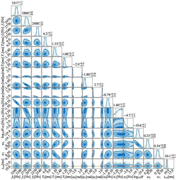
Figure B.1: Full posteriors corresponding to the $t_{\mathrm{col}}=10\,$ms injection shown in Fig. 1. The numerical-relativity simulation is injected into a 2A+ detector network at a distance of 3.04 Mpc with an SLy equation of state and equal-mass $1.35\,\mathrm{M}_{\odot}$ neutron stars. Credible intervals of 68% are shown as dashed blue lines in the one-dimensional posteriors. The injected collapse time is shown by the orange lines in the lower-most panels.

References

- Zhang (2019) B. Zhang, Frontiers of Physics 14, 64402 (2019).
- Ciolfi (2020) R. Ciolfi, General Relativity and Gravitation 52, 59 (2020).
- Tolman (1939) R. C. Tolman, Physical Review 55, 364 (1939).
- Oppenheimer and Volkoff (1939) J. R. Oppenheimer and G. M. Volkoff, Physical Review 55, 374 (1939).
- Breu and Rezzolla (2016) C. Breu and L. Rezzolla, Monthly Notices of the Royal Astronomical Society 459, 646 (2016).
- Weih et al. (2018) L. R. Weih, E. R. Most, and L. Rezzolla, Monthly Notices of the Royal Astronomical Society: Letters 473, L126 (2018).
- Baumgarte et al. (2000) T. W. Baumgarte, S. L. Shapiro, and M. Shibata, The Astrophysical Journal 528, L29 (2000).
- Paschalidis et al. (2012) V. Paschalidis, Z. B. Etienne, and S. L. Shapiro, Physical Review D 86, 064032 (2012).
- Sarin and Lasky (2020) N. Sarin and P. D. Lasky, arXiv e-prints (2020), arXiv:2012.08172 .
- Metzger et al. (2018) B. D. Metzger, T. A. Thompson, and E. Quataert, The Astrophysical Journal 856, 101 (2018).
- Gill et al. (2019) R. Gill, A. Nathanail, and L. Rezzolla, The Astrophysical Journal 876, 139 (2019).
- Murguia-Berthier et al. (2020) A. Murguia-Berthier, E. Ramirez-Ruiz, F. De Colle, A. Janiuk, S. Rosswog, and W. H. Lee, arXiv e-prints (2020), arXiv:2007.12245 .
- Yu et al. (2018) Y.-W. Yu, L.-D. Liu, and Z.-G. Dai, The Astrophysical Journal 861, 114 (2018).
- Zhuge et al. (1994) X. Zhuge, J. M. Centrella, and S. L. McMillan, Physical Review D 50, 6247 (1994).
- Stergioulas et al. (2011) N. Stergioulas, A. Bauswein, K. Zagkouris, and H.-T. Janka, Monthly Notices of the Royal Astronomical Society 418, 427 (2011).
- Takami et al. (2015) K. Takami, L. Rezzolla, and L. Baiotti, Physical Review D 91, 064001 (2015).
- Bernuzzi et al. (2015) S. Bernuzzi, T. Dietrich, and A. Nagar, Physical Review Letters 115, 091101 (2015).
- Martynov et al. (2019) D. Martynov, H. Miao, H. Yang, F. H. Vivanco, E. Thrane, R. Smith, P. Lasky, W. E. East, R. Adhikari, A. Bauswein, A. Brooks, Y. Chen, T. Corbitt, A. Freise, H. Grote, Y. Levin, C. Zhao, and A. Vecchio, Physical Review D 99, 102004 (2019).
- Ackley et al. (2020) K. Ackley, V. B. Adya, P. Agrawal, P. Altin, G. Ashton, M. Bailes, E. Baltinas, A. Barbuio, D. Beniwal, C. Blair, et al., Publications of the Astronomical Society of Australia 37, e047 (2020).
- Easter et al. (2020) P. J. Easter, S. Ghonge, P. D. Lasky, A. R. Casey, J. A. Clark, F. Hernandez Vivanco, and K. Chatziioannou, Physical Review D 102, 043011 (2020).
- Bauswein et al. (2016) A. Bauswein, N. Stergioulas, and H.-T. Janka, European Physical Journal A 52, 56 (2016).
- Bose et al. (2018) S. Bose, K. Chakravarti, L. Rezzolla, B. S. Sathyaprakash, and K. Takami, Physical Review Letters 120, 031102 (2018).
- Tsang et al. (2019) K. W. Tsang, T. Dietrich, and C. Van Den Broeck, Physical Review D 100, 044047 (2019).
- Breschi et al. (2019) M. Breschi, S. Bernuzzi, F. Zappa, M. Agathos, A. Perego, D. Radice, and A. Nagar, Physical Review D 100, 104029 (2019).
- Abbott et al. (2017a) B. P. Abbott, R. Abbott, T. D. Abbott, F. Acernese, K. Ackley, C. Adams, T. Adams, P. Addesso, R. X. Adhikari, V. B. Adya, et al., The Astrophysical Journal 848, L12 (2017a).
- Dietrich et al. (2018) T. Dietrich, D. Radice, S. Bernuzzi, F. Zappa, A. Perego, B. Brueugmann, S. Vivekanandji Chaurasia, R. Dudi, W. Tichy, and M. Ujevic, arXiv e-prints (2018), http://www.computational-relativity.org, arXiv:1806.01625 .
- Dietrich et al. (2017) T. Dietrich, S. Bernuzzi, M. Ujevic, and W. Tichy, Physical Review D 95, 044045 (2017).
- Dietrich and Hinderer (2017) T. Dietrich and T. Hinderer, Physical Review D 95, 124006 (2017).
- Douchin and Haensel (2001) F. Douchin and P. Haensel, Astronomy & Astrophysics 380, 151 (2001).
- Radice et al. (2016) D. Radice, S. Bernuzzi, and C. D. Ott, Physical Review D 94, 064011 (2016).
- Lattimer and Douglas Swesty (1991) J. M. Lattimer and F. Douglas Swesty, Nuclear Physics, Section A 535, 331 (1991).
- Radice (2017) D. Radice, The Astrophysical Journal Letters 838, L2 (2017).
- Abbott et al. (2019a) B. P. Abbott, R. Abbott, T. D. Abbott, F. Acernese, K. Ackley, C. Adams, T. Adams, P. Addesso, R. X. Adhikari, V. B. Adya, et al., Physical Review X 9, 011001 (2019a).
- Abbott et al. (2020) B. P. Abbott, R. Abbott, T. D. Abbott, S. Abraham, F. Acernese, K. Ackley, C. Adams, V. B. Adya, C. Affeldt, M. Agathos, et al., Living Reviews in Relativity 23, 3 (2020).
- LIGO Scientific Collaboration (2020a) LIGO Scientific Collaboration, “Unofficial sensitivity curves (ASD) for aLIGO, Kagra, Virgo, Voyager, Cosmic Explorer, and Einstein Telescope,” (2020a), https://dcc.ligo.org/LIGO-T1500293.
- Hild et al. (2008) S. Hild, S. Chelkowski, and A. Freise, arXiv (2008), arXiv:0810.0604 .
- Punturo et al. (2010) M. Punturo, M. Abernathy, F. Acernese, B. Allen, N. Andersson, K. Arun, F. Barone, B. Barr, M. Barsuglia, M. Beker, et al., Classical and Quantum Gravity 27, 084007 (2010).
- Hild et al. (2011) S. Hild, M. Abernathy, F. Acernese, P. Amaro-Seoane, N. Andersson, K. Arun, F. Barone, B. Barr, M. Barsuglia, M. Beker, et al., Classical and Quantum Gravity 28, 094013 (2011).
- LIGO Scientific Collaboration (2020b) LIGO Scientific Collaboration, “Unofficial sensitivity curves (ASD) for aLIGO, Kagra, Virgo, Voyager, Cosmic Explorer, and Einstein Telescope,” (2020b), http://www.et-gw.eu/index.php/etsensitivities.
- Abbott et al. (2017b) B. P. Abbott, R. Abbott, T. D. Abbott, M. R. Abernathy, K. Ackley, C. Adams, P. Addesso, R. X. Adhikari, V. B. Adya, C. Affeldt, et al., Classical and Quantum Gravity 34, 44001 (2017b), 1607.08697 .
- Adhikari et al. (2019) R. X. Adhikari, S. Ballmer, B. Barish, L. Barsotti, G. Billingsley, D. A. Brown, Y. Chen, D. Coyne, R. Eisenstein, M. Evans, et al., Bulletin of the American Astronomical Society 51 (2019), https://baas.aas.org/pub/2020n7i035.
- LIGO Scientific Collaboration (2016) LIGO Scientific Collaboration, “Exploring the sensitivity of next generation gravitational wave detectors,” (2016), https://dcc.ligo.org/LIGO-P1600143/public, curve_data.txt.
- Ashton et al. (2019) G. Ashton, M. Hübner, P. D. Lasky, C. Talbot, K. Ackley, S. Biscoveanu, Q. Chu, A. Divakarla, P. J. Easter, B. Goncharov, F. Hernandez Vivanco, J. Harms, M. E. Lower, G. D. Meadors, D. Melchor, E. Payne, M. D. Pitkin, J. Powell, N. Sarin, R. J. E. Smith, and E. Thrane, The Astrophysical Journal Supplement 241, 27 (2019).
- Cornish and Littenberg (2015) N. J. Cornish and T. B. Littenberg, Classical and Quantum Gravity 32, 135012 (2015).
- Littenberg and Cornish (2015) T. B. Littenberg and N. J. Cornish, Physical Review D 91, 084034 (2015).
- Chatziioannou et al. (2017) K. Chatziioannou, J. A. Clark, A. Bauswein, M. Millhouse, T. B. Littenberg, and N. Cornish, Physical Review D 96, 124035 (2017).
- Torres-Rivas et al. (2019) A. Torres-Rivas, K. Chatziioannou, A. Bauswein, and J. A. Clark, Physical Review D 99, 044014 (2019).
- Zhang et al. (2021) T. Zhang, J. Smetana, Y. Chen, J. Bentley, D. Martynov, H. Miao, W. E. East, and H. Yang, Physical Review D 103, 044063 (2021).
- The LIGO Scientific Collaboration et al. (2020) The LIGO Scientific Collaboration, the Virgo Collaboration, R. Abbott, T. D. Abbott, S. Abraham, F. Acernese, K. Ackley, A. Adams, C. Adams, R. X. Adhikari, et al., arXiv e-prints (2020), arXiv:2010.14533 .
- Abbott et al. (2017) B. P. Abbott, R. Abbott, T. D. Abbott, F. Acernese, K. Ackley, C. Adams, T. Adams, P. Addesso, R. X. Adhikari, V. B. Adya, and et al., The Astrophysical Journal Letters 851, L16 (2017).
- Abbott et al. (2019b) B. Abbott, R. Abbott, T. Abbott, F. Acernese, K. Ackley, C. Adams, T. Adams, P. Addesso, R. Adhikari, et al., LIGO Scientific Collaboration, and Virgo Collaboration, The Astrophysical Journal 875, 160 (2019b).