Graph-MLP: Node Classification without Message Passing in Graph

Abstract

Graph Neural Network (GNN) has been demonstrated its effectiveness in dealing with non-Euclidean structural data. Both spatial-based and spectral-based GNNs are relying on adjacency matrix to guide message passing among neighbors during feature aggregation. Recent works have mainly focused on powerful message passing modules, however, in this paper, we show that none of the message passing modules is necessary. Instead, we propose a pure multilayer-perceptron-based framework, Graph-MLP with the supervision signal leveraging graph structure, which is sufficient for learning discriminative node representation. In model-level, Graph-MLP only includes multi-layer perceptrons, activation function, and layer normalization. In the loss level, we design a neighboring contrastive (NContrast) loss to bridge the gap between GNNs and MLPs by utilizing the adjacency information implicitly. This design allows our model to be lighter and more robust when facing large-scale graph data and corrupted adjacency information. Extensive experiments prove that even without adjacency information in testing phase, our framework can still reach comparable and even superior performance against the state-of-the-art models in the graph node classification task.

1 Introduction

Deep learning has provided the powerful capacity for machine learning tasks in recent years. Besides the data in the euclidean space, there is an increasing number of graph structured data in the non-euclidean domains. To cope with the graph-related tasks that generally exist in different fields, such as computer vision (Xu et al., 2017) (Yang et al., 2018), traffic (Zhang et al., 2018) (Li et al., 2017), recommender systems (He et al., 2020a), Graph Neural Networks (GNNs) have drawn more and more research interests.

Among those GNNs, how to build an effective and efficient message passing module between neighbors has been the main focus in order to boost the performance. As a pioneer, Graph Convolutional Network (GCN) (Kipf and Welling, 2016) sums up the neighbor features to obtain the new node feature. Graph Attention Network (GAT) (Veličković et al., 2017) learns attention values among connected nodes to adaptive pass the message and update node features, and multiple multi-head attention layers are stacked.

Besides sophisticated GNN structures and enhanced performance, there has been a trend to design simpler and more efficient GNN structures. For instance, SGC (Wu et al., 2019) reduces excess complexity through successively removing activation layer and using the pre-computed $r^{th}$ power of adjacency matrix. However, they all share the de facto design that graph structure information is explicitly utilized in message passing modules to aggregate features. Considering the time consumption, a natural question is whether we can remove the redundant message passing modules.

In this paper, we aim to learn the structural node representation without explicit message passing. We propose a novel alternative to GNNs, Graph-MLP, where we implicitly use supervision signals from node connection information to guide a pure MLP-based model for graph node classification. In Graph-MLP, linear layers are combined with activation function, layer normalization, and dropout layers to compose our model structure. The message passing between neighbors through feature aggregation is completely abandoned. Instead, a novel Neighboring Contrastive (NContrast) loss is proposed to implicitly incorporate graph structure into feature transformation. More specifically, for each node, its i-hop neighbors are treated as positive samples and other unconnected nodes are regarded as negative samples. The distance between the selected node against the positive/negative would drew/pushed closer/farther.

The advantages of Graph-MLP over previous GNNs exist in two folds. 1) Higher computation efficiency via bypassing message passing in feed-forward propagation: Since our model structure does not require explicit message passing as the conventional graph models, this allows us more freedom in choosing simpler base model i.e. MLP. A Simple and light base model is often required in lots of applications. 2) Robustness against corrupted edges during inference: In real-world applications, it often happens that some new samples are not connected to any node in the existing graph, such as "a new social network platform user to a recommendation system". And sometimes, there might be some noise in collected connection information. Then conventional GNNs are incompetent in providing recommendations due to the vacant or noist adjacency information. However, adjacency connection is not needed in the inference phase of Graph-MLP framework. Because our Ncontrast loss allows Graph-MLP to learn a structural-aware nodes’ feature transformation. Thus Graph-MLP can still provide consistent recommendations despite the user node’s missing connections.

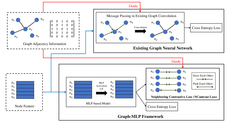
Figure 1: Diagram of Graph-MLP. GNNs take the adjacency matrix and node feature as input for message passing on node classification task. Graph-MLP takes node feature as input and utilizes the adjacency matrix in NContrast loss.

To demonstrate the Graph-MLP’s superiority, we conduct extensive experiments on two points: (1) Graph-MLP can achieve comparative performance as GNNs with higher efficiency in three node classification benchmarks. (2) Graph-MLP’s robustness in feature transformation during inference with corrupted connection information.

Our contributions are summarized as follows:

• A simple MLP-based graph learning framework (Graph-MLP) without message passing modules. To our best knowledge, it is the first deep learning framework to effectively perform graph node classification task without explicit message passing modules.

• A novel Neighboring Contrastive loss to implicitly incorporate graph structure into node representation learning.

• Experimental results show that Graph-MLP can achieve comparable or even superior performance on node classification tasks with higher efficiency. When adjacency information is corrupted or missing in the inferencing time, Graph-MLP robustly maintains consistent performance.

The rest of the paper is structured as follows. Related works are reviewed in Section 2. Necessary preliminaries and Graph-MLP framework are introduced in Section 3. Extensive experiments are reported in Section 4.

2 Related Work

Graph Neural Networks

GCN (Kipf and Welling, 2016) first generalizes classic Convolutional Neural Net-works (CNNs) from euclidean domain to graph domain. Then follow-up works can be divided into SpatialGCNs and Spectral GCNs. (You et al., 2020) surveys a wide range of GNN design spaces for different tasks. It also includes pragmatic guidelines in designing GNNs for several tasks. There is also some other form of graph neural networks concentrating on hypergraphs (Feng et al., 2019).To help GNN learning representations on Riemannian manifolds, (Chami et al., 2019) and (Liu et al., 2019) utilize hyperbolic embedding to facilitate learning.

Multilayer Perceptron

Recently, MLPs are attracting vision reserch to design more general and simple architecture. (Tolstikhin et al., 2021) (Melas-Kyriazi, 2021) design MLP based network and performs as well as prevalent vision networks (Dosovitskiy et al., 2020). (Touvron et al., 2021) proposed residual blocks consisting of feed-forward network and interaction layer. (Ding et al., 2021) use re-parameterization technique to add local prior into MLP to make it powerful for image recognition. These work pave the way for applying MLP-based model to different research domains. And they demonstrate the potential of MLP-based models against other complicated models.

Contrastive Learning

Contrastive learning is widely applied in self-supervised learning such as (Chen et al., 2020a) (Chen et al., 2020b) (He et al., 2020b) (Chen et al., 2020c) (Grill et al., 2020). Contrastive learning is also used in supervised way like (Khosla et al., 2021). In natural language processing, (Gunel et al., 2020) use supervised contrastive learning to help to pre-train a large language model on an auxiliary task. There are also self-supervised learning applied on graph learning. Exhaustive information is referred to (Jin et al., 2020).

3 Method

Following GCNs (Kipf and Welling, 2016), we introduce our Graph-MLP in the context of node classification task. In this task, a graph consisted of both labeled and unlabled nodes is input into a model, and the output is the prediction of unlabeled nodes. For a given graph $\mathcal{G}$, we can represent it as $\mathcal{G}=(\mathcal{V},\mathbf{A})$, where the vertex set is $\mathcal{V}$ containing nodes $\left\{v_{1},\ldots,v_{n}\right\}$ and $\mathbf{A}\in\mathbb{R}^{n\times n}$ is the adjacency matrix where $a_{ij}$ denotes the edge weight between nodes $v_{i}$ and $v_{j}$. In the graph $\mathcal{G}$, we denote the node feature matrix as $\mathbf{X}\in\mathbb{R}^{n\times d}$ where the feature vector of each node $v_{i}$ is $\mathrm{x}_{i}\in\mathbb{R}^{d}$. Each node belongs to one category of $C$ classes with a one-hot label, $\mathbf{y}_{i}\in\{0,1\}^{C}$. The node classification task requires the model to give predicted labels of the test nodes.

3.1 Revisiting GNNs

In vanilla GCN, MLPs and summation operation over connected nodes are combined together to propagate features among neighbors.

$$\mathbf{X}^{(l+1)}=\sigma\left(\widehat{A}\mathbf{X}^{(l)}W^{(l)}\right)$$ (1)

where $\mathbf{X}^{(0)}=\mathbf{X}$ and $\mathbf{X}^{(l)}$ means the $l^{th}$ layer features. $W^{l}$ is the weight of the single linear layer of the $l^{th}$ layer and $\sigma$ is an activation function. The normalized adjacency matrix $\widehat{A}$ is utilized to pass messages between neighbors.

$$\widehat{A}=\mathbf{D}^{-\frac{1}{2}}\left(A+I\right)\mathbf{D}^{-\frac{1}{2}}$$ (2)

where $I$ denotes self-connection, $\mathbf{D}$ is a diagonal matrix and $\mathbf{D}_{(i,i)}=\sum_{j}\widetilde{A}_{(i,j)}$.

In follow-up works, various ways of passing messages between neighbors have been proposed. For instance, GAT employs an attention module to dynamically learn the attention weight of message passing among neighbors. GGNN (Li et al., 2015) incorporate GRU (Chung et al., 2014) into message passing process to allow the interaction between memory and current feature.

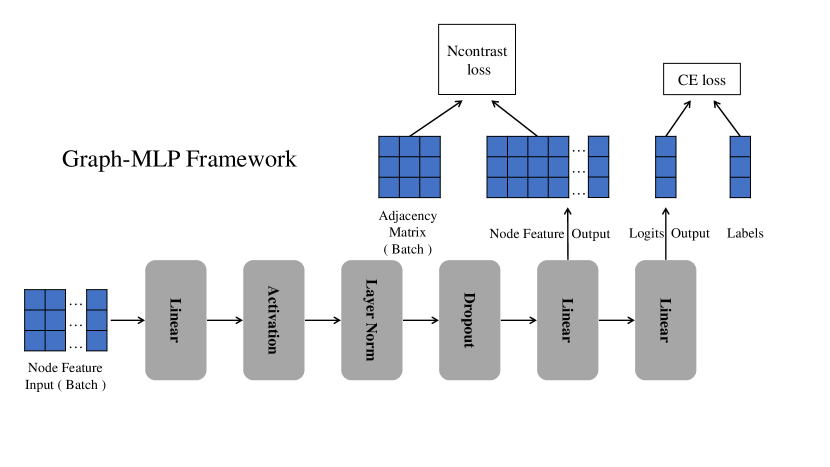
Figure 2: The framework of Graph-MLP.

3.2 Graph-MLP

Previous graph models heavily focus on leveraging message passing among neighbors. By their design, graph structure is explicitly learned in feed-forward feature propagation. Those sophisticated message passing often lead to complex structure and heavy computation. In this work, we creatively explore a new perspective to learn node feature transformation without explicit message passing. In structure level, despite its simple design, we use a pure MLP-based model. To compensate for its light structure in graph modelling, we combine it with a novel contrastive loss to supervise its learning of node feature transformation.

In the following, we would introduce our proposed framework, Graph-MLP in three perspectives: 1) The MLP-based model structure; 2) The Neighbouring Contrastive (NContrast) loss for supervising node feature transformation. 3) Training and Inferencing of Graph-MLP.

MLP-based Structure

Following the common design, our MLP-based structure consists of linear layers followed by activation, normalization, and dropout as in Figure 2. More specifically, a linear-activation-layer normalization-dropout block is utilized and two following additional linear layers serve as the prediction heads. For activation, we use Gelu (Hendrycks and Gimpel, 2016). Layernorm (Ba et al., 2016) is applied instead of batch normalization for the training stability. Dropout (Srivastava et al., 2014) is to avoid over-fitting. The second last linear layer is supervised for feature transformation with our proposed NContrast loss and, differently, the last linear layer is guided for learning node classification. The entire model can be formulated as:

$$\mathbf{X}^{(1)}=Dropout\left(LN\left(\sigma\left(\mathbf{X}W^{0}\right)\right)\right)$$ (3)

$$\mathbf{Z}=\mathbf{X}^{(1)}W^{1}$$ (4)

$$\mathbf{Y}=\mathbf{Z}W^{2}$$ (5)

where $\mathbf{Z}$ will be used for NContrast loss, and $\mathbf{Y}$ will be used for classification loss. Compared with Equation 1 and other GNNs, Graph-MLP does not require the normalized adjacency matrix $\widehat{A}$ and corresponding message passing step.

Neighbouring Contrastive Loss

For enabling the feature extraction with graph connection information, it is intuitive that connected nodes should be similar to each other and unconnected ones should be far away in feature space. This aligns well with the idea inside contrastive learning. With such motivation, we propose a Neighbouring Contrastive loss which enables an MLP-based model to learn graph node connections without explicit messaging passing modules.

In NContrast loss, for each node, its $r$-hop neighbors are regarded as the positive samples, while the other nodes are sampled as the negative ones. The loss encourages positive samples to be closer to the target node and pushes negative samples away from the target one in terms of feature distance. In details, NContrast loss for the $i^{th}$ node can be formulated as:

$$\ell_{i}=-\log\frac{\sum_{j=1}^{B}\mathbf{1}_{[j\neq i]}\gamma_{ij}\exp\left(\operatorname{sim}\left(\boldsymbol{z}_{i},\boldsymbol{z}_{j}\right)/\tau\right)}{\sum_{k=1}^{B}\mathbf{1}_{[k\neq i]}\exp\left(\operatorname{sim}\left(\boldsymbol{z}_{i},\boldsymbol{z}_{k}\right)/\tau\right)}$$ (6)

where $\operatorname{sim}$ denotes the cosine similarity and $\tau$ denotes the temperature parameter. $\gamma_{ij}$ means the strength of connection between node $i$ and $j$. We compute it as the $r^{th}$ power of normalized adjacency matrix $\widehat{A}^{r}$: $\gamma_{ij}=\widehat{A}^{r}_{ij}$. $\gamma^{ij}$ gets non-zero values only if node $j$ is the $r$-hop neighbor of node $i$.

$$\gamma_{ij}\begin{cases}=0,&\text{node $j$ is the $r$-hop neighbor of node $i$}\\ \neq 0,&\text{node $j$ is not the $r$-hop neighbor of node $i$ }\\ \end{cases}$$

Besides the NContrast loss, we also have a traditional cross-entropy (CE) loss for node classification, as in (Kipf and Welling, 2016). It’s noted that NContrast loss is applied after the second last layer and CE loss is on top of the last layer. In total, we define the final loss of Graph-MLP as a combination of both:

$$loss_{NC}=\alpha\frac{1}{B}\sum_{i=1}^{B}\ell_{i}$$ (7)

$$loss_{final}=loss_{CE}+loss_{NC}$$ (8)

where $loss_{CE}$ is the cross entropy loss. $\alpha$ is the weighting coefficient to balance the those two losses.

Algorithm 1 Graph-MLP training

Input: Feature matrix $\mathbf{X}$ and $r^{th}$ power of adjacency matrix $\widehat{A}^{r}$. The train/validation/test index. Hyperparameter $B$, $\alpha$, $\tau$. Trainable model parameters $\theta$. Training iterations $T$.
Output: Optimized model parameters $\theta$.

1:

2:$t\leftarrow 0$

3:while $t<T$ do

4:     Sample the input batch node feature matrix $\mathbf{X}[Id_{B},:]$ and the input batch adjacency matrix $\widetilde{A}[Id_{B},Id_{B}]$

5:     Compute $loss$ with Eq. 7

6:     Perform backpropagation with $loss$ and update the model parameter $\theta$

7:end while

Training

The entire model is trained in an end-to-end manner. The feedforward of our model does not require adjacency matrix and we only reference graphical structure when computing the loss during training. This allows us much more flexibility against the conventional graph modelling that our framework can be trained with batches without the full graph information (Kipf and Welling, 2016). As shown in Algorithm 1, in each batch, we randomly sample $B$ nodes and take the corresponding adjacency information $\widehat{A}\in\mathbb{R}^{B\times B}$ and node features $\mathbf{X}\in R^{\mathbb{R}\times d}$. It’s noted that, in Equation 3.2, for some node $i$, it may happen that no positive sample is in the batch, due to the randomness of batch sampling. In that case, we will remove the loss for node $i$. And we find our model robust to the ratio of positive and negative samples, without specifically tuned ratio. A better batch sampling method and the fusion of Graph-MLP and works like GraphSAGE (Hamilton et al., 2017) are still remained for future exploration.

Inference

During the inferencing, the conventional graph modellings e.g. GNNs need both the adjacency matrix and node features as inputs. Differently, our MLP-based method only requires node features as input. Hence, when adjacency information is corrupted or missing, Graph-MLP could still deliver consistently reliable results. In the conventional graph modelling, graph information is embedded in adjacency matrix in input. For those models, the learning of graph node transformation heavily relies on internal message passing which is sensitive to connections in each adjacency matrix input. However, our supervision of graphical structure is applied on the loss level. Thus our framework is able to learn a graph-structured distribution during node feature transformation without feed-forward message passing. This allows our model to be less sensitivity to specific connections during inference.

4 Experiments

4.1 Datasets and Experiment Setting

In this section, we evaluate the performance of Graph-MLP against the prevalent GNN models on the three popular citation network datasets in node classification as in Table 2. In semi-supervised node classification, $140/500/1\,000$ nodes are used for training/validation/testing in Cora. 120/500/1, 000 nodes are used for training/validation/testing in Citeseer. 60/500/1, 000 nodes are used for training/validation/testing in Pubmed.

Dataset	Cora	Citeseer	Pubmed
Node	2,708	3,327	19,717
Edge	5,429	4,732	44,338
Feature	1,433	3,703	500
Class	7	6	3

Table 1: Statistics of three citation network datasets.

	Cora	Citeseer	Pubmed
DeepWalk	$70.7$	$51.4$	$76.8$
AdaLNet	$80.4$	$68.7$	$78.1$
LNet	$79.5$	$66.2$	$78.3$
GCN	$81.5$	$70.3$	$79.0$
GAT	$83.0$	$72.5$	$79.0$
DGI	$\mathbf{82.3}$	$71.8$	$76.8$
SGC	$81.0$	$71.9$	$78.9$
MLP ($\alpha$=0)	$57.8$	$54.7$	$73.3$
Graph-MLP	$79.5$	$\mathbf{73.1}$	$\mathbf{79.7}$

Table 2: Test accuracy (%) on citation network datasets. The scores in the table are obtained by averaging over 10 runs for each experiment.

Graph-MLP Network Structure We use the network with the same structure as Figure 2. We set the hidden dimension $d$=256 in each linear layer. The dropout rate is 0.6 fixed. We use Gelu (Hendrycks and Gimpel, 2016) as the activation function.

Training Setups The training iterations for each data set is fixed with 400. We use Adam (Kingma and Ba, 2014) as the optimizer. We also sweep the learning rate in the range of [0.001,0.01,0.05,0.1], the weight decay in the range of [5e-4,5e-3], the batch size in the range of [2000,3000], the temperature parameter $\tau$ in the range of [0.5,1.0,2.0], the $r$ parameter (for computing $r^{th}$ power of adjacency matrix) in the range of [2,3,4] and the $\alpha$, as in Equation 7, in the range of [0,1,10,100] (when $\alpha$ is 0, the Graph-MLP degrade into vanilla MLP).

Evaluating Setups We report the final testing results based on the best performed model on validation results. Each result is run 10 times with random initialization.

Performance on citation networks node classification dataset: We compare our results versus several the state-of-the-art graph learning methods including LNet (Liao et al., 2019), AdaLNet (Liao et al., 2019), DeepWalk (Perozzi et al., 2014), DGI (Velickovic et al., 2019), GCN (Kipf and Welling, 2016) and SGC (Wu et al., 2019). In Table 2, Graph-MLP can achieve the state-of-the-art performance on Citeseer and Pubmed among the all. Even on Cora, our results are also comparable with other methods. The reason of a slightly lower performance on Cora might be due to the scale of graph. A smaller graph may not be able to provide enough genearl contrastive supervision compared with larger graphs. Compared with the original vanilla MLP (with $\alpha$=0, Graph-MLP behaves the same as original MLP), Graph-MLP improves by 21.7%, 18.4%, and 6.4% respectively on Cora, Citeseer, and Pubmed. This substantial improvement clearly demonstrates the contribution from our proposed NContrast loss.

4.2 A Deeper Understanding of Graph-MLP

Efficiency of Graph-MLP versus GNNs To compare Graph-MLP and GCN (Kipf and Welling, 2016) in training and testing behavior, we add message passing modules e.g. graph convolution before the first and second linear layer in our MLP-based structure to transform it to a two-layer GCN as in (Kipf and Welling, 2016). In this way, we can compare the training and testing efficiency fairly with only message passing layer being a variable. For the common hyperparameters of Graph-MLP and GCN, we use a Adam optimizer with the learning rate as 0.01, the weight decay as 5e-4 and the hidden dimension as 256. For our Graph-MLP’s specific setting, we set the $\alpha$ to be 1, the batch size to be 2000, $r$ to be 2 in all three datasets. The comparison is evaluated regarding training converge time and inferencing time. It is noted that batch sampling time is also counted in Graph-MLP’s training coverage time.

In Figure 3, we find that Graph-MLP can achieve better results on Citeseer and Pubmed with a quicker converge speed compared with GCN. Additionally, our testing accuracy is more stable and smooth compared with GCN’s which demonstrates an inconsistent performance mixed with fluctuations in the testing accuracy, especially as shown in the middle and the rightmost subfigures in Figure. 3. In Cora, GCN converges earlier, however, the final converged performance of the two is comparable. The reason behind may still be the smaller scale of Cora dataset. Furthermore, we compare the inferencing time for the testing nodes. GCN needs both the adjacency matrix and the node features to be input, but our Graph-MLP only requires testing node features. We run the inferencing process 100 times and average the recordings to remove the randomness. The time consumption for testing is listed in Table 3. We can see that GCN’s inferencing time will increase with the larger number of nodes in the whole graph because of multiplication of the larger adjacency matrix. Nevertheless, with credits to the simiplicity of Graph-MLP, its inferencing time is much faster and only depends on the number of testing nodes. Overall, Graph-MLP shows superior efficiency in both training and inferencing.

	Cora	Citeseer	Pubmed
GCN	$0.000917$	$0.001918$	$0.010107$
Graph-MLP	$0.000276$	$0.000262$	$0.000262$

Table 3: Testing time (s) for Graph-MLP and GCN.

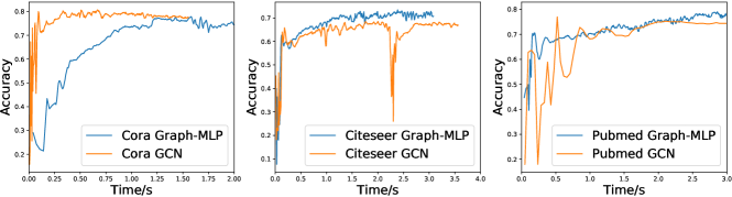
Figure 3: Accuracy along training time of Graph-MLP and GCN.

Ablation Study about Hyperparameters To have a deeper understanding about the effect of hyperparameters in Graph-MLP, we give an exhaustive analysis on them as in Figure 4. Among the hyperparameters $\tau$, $r$, $B$, $\alpha$, learning rate, and weight decay. We find that: (1) $\tau$, $r$, $B$ are trivial hyperparameters for their values’ change doesn’t affect the distribution of the results much. In another aspect, it shows that Graph-MLP is robust to the mentioned hyperparameters. (2) As $\alpha$’s value gets bigger from 1 to 10, accuracy gets consistent improvement on Cora and Pubmed. However, with $\alpha$ as 100, performance on Cora and Pubmed drops a little. On Citeseer, with $\alpha$ from 1 to 100, the performance keeps improving and gives the best one around 100. (3) Learning rate with 0.01 can usually perform well, which is a recommending default setting. Also, observing that weight decay with 5e-3 is slightly better than 5e-4, we hypothesize that our Graph-MLP may need a stronger regularization.

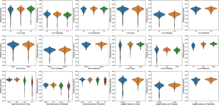
Figure 4: Ablation study on the hyperparameters ( including $\tau$, $r$, $B$, $\alpha$, learning rate, and weight decay) on citation network datasets. A hyperparameter with higher and more condensed distribution represents its superiority over its counterpart.

Visualization of Embeddings In order to have a visual understanding of how NContrast loss helps vanilla MLP, we visualize the feature embedding of $\mathbf{Z}$ with t-SNE (Van der Maaten and Hinton, 2008). Here, learning rate is 0.01, weight decay is 5e-4, $\alpha$ ranges from [0.0, 1.0, 10.0], the hidden dimension $d$ is 256, batch size is 2000, $r$ is 2, and $\tau$ is 2. The t-SNE visualization results are plotted as in Figure 5. For example, in Cora, as $\alpha$ grows bigger from 0 to 100, the node embeddings of the same class become cloaser and the embeddings of different classes are pushed farther from each other. Visualized results on Citeseer and Pubmed also reveal the similar effect.

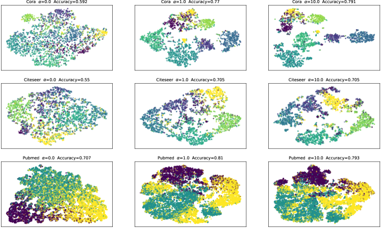
Figure 5: t-SNE visualization of feature embedding of citation networks. We plot the whole nodes feature produce from the converged model.

4.3 Robustness against Corrupted Connection in Inference

In real world applications, it oftens happens that, testing node features and corrupted adjacency information are provided in inference. Then, how will the GCN and Graph-MLP behave in the testing case with corrupted adjacency information? To simulate the corrupted data that may exist in the real word scenarios, we add noises on the adjacency matrix in testing. We define a corruption ratio $\delta$ and the corruption $mask$ to determine positions in the adjacency matrix that need to be corrupted. The corrupted adjacency matrix can be formulated as:

$$A_{corr}=A\otimes mask+(1-mask)\otimes\mathbb{N}$$ (9)

$$mask\begin{cases}=1,&p=1-\delta\\ =0,&p=\delta\\ \end{cases}$$ (10)

where values in $mask\in n\times n$ will be 1/0 under the probability of $1-\delta$/$\delta$. Each item in $\mathbb{N}\in n\times n$ will also be 1/0 under the probability of 0.5/0.5. In total, the formula means that we randomly add or remove edges for a $\delta$ ratio of the adjacency connections, in order to mimic the noises. In our experiments, we try with $\delta$ to be 0.01 or 0.1 and compare the testing performance of GCN and Graph-MLP. In Figure 6, we can see that Graph-MLP’s performance is free from the influence of corruption in the adjacency matrix. But even a tiny disturbance (setting $\delta$ equals 0.01 so only 1 percent of adjacency information is corrupted) will result in the drastic performance degradation with GCN. Therefore, the Graph-MLP shows great robustness against the corruption in adjacency information.

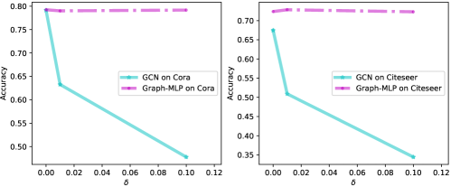
Figure 6: Results with corruption on adjacency matrix. For every $\delta$, both GCN and Graph-MLP are trained and tested three times, and averaged accuracy is shown.

5 Conclusion

In this paper, we propose a novel MLP-based method, Graph-MLP for learning graph node feature distribution. Despite its light structure, to our best knowledge, it is the first deep learning framework to effectively perform graph node classification task without explicit message passing modules. For further supervising our model in term of learning graph node transformation, we propose the NContrast loss to enable learning the structural node distribution without explicit referencing to graph connections i.e. adjacency matrix in feedforward. This flexibility in learning contextual knowledge without the message passing modules enables our mode to inference with even corrupted edge information. Our extensive experiments showcase that Graph-MLP is able to deliver comparable and even superior results against the state-of-the-art in node classification tasks with a much simpler and lighter structure.

References

- Xu et al. [2017] Danfei Xu, Yuke Zhu, Christopher B Choy, and Li Fei-Fei. Scene graph generation by iterative message passing. In Proceedings of the IEEE conference on computer vision and pattern recognition, pages 5410–5419, 2017.
- Yang et al. [2018] Jianwei Yang, Jiasen Lu, Stefan Lee, Dhruv Batra, and Devi Parikh. Graph r-cnn for scene graph generation. In Proceedings of the European conference on computer vision (ECCV), pages 670–685, 2018.
- Zhang et al. [2018] Jiani Zhang, Xingjian Shi, Junyuan Xie, Hao Ma, Irwin King, and Dit-Yan Yeung. Gaan: Gated attention networks for learning on large and spatiotemporal graphs. arXiv preprint arXiv:1803.07294, 2018.
- Li et al. [2017] Yaguang Li, Rose Yu, Cyrus Shahabi, and Yan Liu. Diffusion convolutional recurrent neural network: Data-driven traffic forecasting. arXiv preprint arXiv:1707.01926, 2017.
- He et al. [2020a] Xiangnan He, Kuan Deng, Xiang Wang, Yan Li, Yongdong Zhang, and Meng Wang. Lightgcn: Simplifying and powering graph convolution network for recommendation. In Proceedings of the 43rd International ACM SIGIR Conference on Research and Development in Information Retrieval, pages 639–648, 2020a.
- Kipf and Welling [2016] Thomas N Kipf and Max Welling. Semi-supervised classification with graph convolutional networks. arXiv preprint arXiv:1609.02907, 2016.
- Veličković et al. [2017] Petar Veličković, Guillem Cucurull, Arantxa Casanova, Adriana Romero, Pietro Lio, and Yoshua Bengio. Graph attention networks. arXiv preprint arXiv:1710.10903, 2017.
- Wu et al. [2019] Felix Wu, Tianyi Zhang, Amauri Holanda de Souza Jr. au2, Christopher Fifty, Tao Yu, and Kilian Q. Weinberger. Simplifying graph convolutional networks, 2019.
- You et al. [2020] Jiaxuan You, Zhitao Ying, and Jure Leskovec. Design space for graph neural networks. Advances in Neural Information Processing Systems, 33, 2020.
- Feng et al. [2019] Yifan Feng, Haoxuan You, Zizhao Zhang, Rongrong Ji, and Yue Gao. Hypergraph neural networks. In Proceedings of the AAAI Conference on Artificial Intelligence, volume 33, pages 3558–3565, 2019.
- Chami et al. [2019] Ines Chami, Rex Ying, Christopher Ré, and Jure Leskovec. Hyperbolic graph convolutional neural networks. Advances in neural information processing systems, 32:4869, 2019.
- Liu et al. [2019] Qi Liu, Maximilian Nickel, and Douwe Kiela. Hyperbolic graph neural networks, 2019.
- Tolstikhin et al. [2021] Ilya Tolstikhin, Neil Houlsby, Alexander Kolesnikov, Lucas Beyer, Xiaohua Zhai, Thomas Unterthiner, Jessica Yung, Andreas Steiner, Daniel Keysers, Jakob Uszkoreit, Mario Lucic, and Alexey Dosovitskiy. Mlp-mixer: An all-mlp architecture for vision, 2021.
- Melas-Kyriazi [2021] Luke Melas-Kyriazi. Do you even need attention? a stack of feed-forward layers does surprisingly well on imagenet, 2021.
- Dosovitskiy et al. [2020] Alexey Dosovitskiy, Lucas Beyer, Alexander Kolesnikov, Dirk Weissenborn, Xiaohua Zhai, Thomas Unterthiner, Mostafa Dehghani, Matthias Minderer, Georg Heigold, Sylvain Gelly, Jakob Uszkoreit, and Neil Houlsby. An image is worth 16x16 words: Transformers for image recognition at scale, 2020.
- Touvron et al. [2021] Hugo Touvron, Piotr Bojanowski, Mathilde Caron, Matthieu Cord, Alaaeldin El-Nouby, Edouard Grave, Armand Joulin, Gabriel Synnaeve, Jakob Verbeek, and Hervé Jégou. Resmlp: Feedforward networks for image classification with data-efficient training, 2021.
- Ding et al. [2021] Xiaohan Ding, Xiangyu Zhang, Jungong Han, and Guiguang Ding. Repmlp: Re-parameterizing convolutions into fully-connected layers for image recognition, 2021.
- Chen et al. [2020a] Ting Chen, Simon Kornblith, Mohammad Norouzi, and Geoffrey Hinton. A simple framework for contrastive learning of visual representations. In International conference on machine learning, pages 1597–1607. PMLR, 2020a.
- Chen et al. [2020b] Ting Chen, Simon Kornblith, Kevin Swersky, Mohammad Norouzi, and Geoffrey Hinton. Big self-supervised models are strong semi-supervised learners, 2020b.
- He et al. [2020b] Kaiming He, Haoqi Fan, Yuxin Wu, Saining Xie, and Ross Girshick. Momentum contrast for unsupervised visual representation learning, 2020b.
- Chen et al. [2020c] Xinlei Chen, Haoqi Fan, Ross Girshick, and Kaiming He. Improved baselines with momentum contrastive learning, 2020c.
- Grill et al. [2020] Jean-Bastien Grill, Florian Strub, Florent Altché, Corentin Tallec, Pierre H. Richemond, Elena Buchatskaya, Carl Doersch, Bernardo Avila Pires, Zhaohan Daniel Guo, Mohammad Gheshlaghi Azar, Bilal Piot, Koray Kavukcuoglu, Rémi Munos, and Michal Valko. Bootstrap your own latent: A new approach to self-supervised learning, 2020.
- Khosla et al. [2021] Prannay Khosla, Piotr Teterwak, Chen Wang, Aaron Sarna, Yonglong Tian, Phillip Isola, Aaron Maschinot, Ce Liu, and Dilip Krishnan. Supervised contrastive learning, 2021.
- Gunel et al. [2020] Beliz Gunel, Jingfei Du, Alexis Conneau, and Ves Stoyanov. Supervised contrastive learning for pre-trained language model fine-tuning. arXiv preprint arXiv:2011.01403, 2020.
- Jin et al. [2020] Wei Jin, Tyler Derr, Haochen Liu, Yiqi Wang, Suhang Wang, Zitao Liu, and Jiliang Tang. Self-supervised learning on graphs: Deep insights and new direction. arXiv preprint arXiv:2006.10141, 2020.
- Li et al. [2015] Yujia Li, Daniel Tarlow, Marc Brockschmidt, and Richard Zemel. Gated graph sequence neural networks. arXiv preprint arXiv:1511.05493, 2015.
- Chung et al. [2014] Junyoung Chung, Caglar Gulcehre, KyungHyun Cho, and Yoshua Bengio. Empirical evaluation of gated recurrent neural networks on sequence modeling. arXiv preprint arXiv:1412.3555, 2014.
- Hendrycks and Gimpel [2016] Dan Hendrycks and Kevin Gimpel. Gaussian error linear units (gelus). arXiv preprint arXiv:1606.08415, 2016.
- Ba et al. [2016] Jimmy Lei Ba, Jamie Ryan Kiros, and Geoffrey E Hinton. Layer normalization. arXiv preprint arXiv:1607.06450, 2016.
- Srivastava et al. [2014] Nitish Srivastava, Geoffrey Hinton, Alex Krizhevsky, Ilya Sutskever, and Ruslan Salakhutdinov. Dropout: a simple way to prevent neural networks from overfitting. The journal of machine learning research, 15(1):1929–1958, 2014.
- Hamilton et al. [2017] William L Hamilton, Rex Ying, and Jure Leskovec. Inductive representation learning on large graphs. arXiv preprint arXiv:1706.02216, 2017.
- Kingma and Ba [2014] Diederik P Kingma and Jimmy Ba. Adam: A method for stochastic optimization. arXiv preprint arXiv:1412.6980, 2014.
- Liao et al. [2019] Renjie Liao, Zhizhen Zhao, Raquel Urtasun, and Richard S. Zemel. Lanczosnet: Multi-scale deep graph convolutional networks, 2019.
- Perozzi et al. [2014] Bryan Perozzi, Rami Al-Rfou, and Steven Skiena. Deepwalk: Online learning of social representations. In Proceedings of the 20th ACM SIGKDD international conference on Knowledge discovery and data mining, pages 701–710, 2014.
- Velickovic et al. [2019] Petar Velickovic, William Fedus, William L Hamilton, Pietro Liò, Yoshua Bengio, and R Devon Hjelm. Deep graph infomax. In ICLR (Poster), 2019.
- Van der Maaten and Hinton [2008] Laurens Van der Maaten and Geoffrey Hinton. Visualizing data using t-sne. Journal of machine learning research, 9(11), 2008.