A new construction for sublevel set persistence

Abstract

We construct a filtered simplicial complex $(X_{L},f_{L})$ associated to a subset $X\subset\mathbb{R}^{d}$, a function $f:X\rightarrow\mathbb{R}$ with compactly supported sublevel sets, and a collection of landmark points $L\subset\mathbb{R}^{d}$. The persistence values $f_{L}(\Delta)$ are defined as the minimizing values of a family of constrained optimization problems, whose domains are certain higher order Voronoi cells associated to $L$. We prove that $H_{k}^{a,b}(X_{L})\cong H^{a,b}_{k}(X)$ in the case when $X=\mathbb{R}^{d}$ and $f$ is smooth, the landmarks are sufficiently dense, and $a<b$ are generic. We show that the construction produces desirable results in some examples.

1 Introduction

Let $f:X\rightarrow\mathbb{R}$, and let $X(a)=f^{-1}(-\infty,a]$ be the sublevel set with the induced topology. The $k$th persistent homology group $H^{a,b}_{k}(X)$ is defined as the image of the homomorphism

$$i^{a,b}_{k}:H_{k}(X(a))\rightarrow H_{k}(X(b))$$ (1)

which is induced from the inclusion map $i^{a,b}:X(a)\rightarrow X(b)$, defined for $a\leq b$.

The homology groups in (1) have several advantages over distance-based persistent homology, but are generally difficult to compute, particularly in higher dimensions. One application of sublevel set persistence is to topological data analysis, which involves computing the superlevel set persistence of a suitable density estimator $\rho$ (or the sublevel set persistence of $-\log(\rho)$). In a seminal paper [6], the authors applied zeroth dimensional superlevel set persistence to define a novel clustering scheme, which provably computed the correct number of clusters, in a mathematically precise sense. Another area where sublevel set persistence has been well-suited is time series analysis, see for instance [7, 8, 15, 17, 18, 20]. The higher dimensional case has been studied using the Morse-Smale complex [11] in the context of grayscale images, which has also been applied to topics such as energy landscapes in particle systems [14]. For other applications and references, see also [1, 2, 3, 4, 5, 10, 22].

We construct a filtered complex $(X_{L},f_{L})$ associated to a subset $X\subset\mathbb{R}^{d}$, a function $f:X\rightarrow\mathbb{R}$ which is bounded below, and a set of landmark points $L=\{p_{1},...,p_{n}\}\subset X$. We have a simplex $\Delta=\{i_{0},...,i_{k}\}\in X_{L}$ if certain higher order Voronoi cells corresponding to the $(k+1)!$ ways of ordering the elements of $\Delta$ are nonempty, and $f_{L}(\Delta)$ is determined by the minimum values of $f$ over those regions, which may be practically obtained using optimization software. We consider the case of $X\subset\mathbb{R}^{d}$, though this construction may be readily extended to a metric space with a locally convex metric, or to a space which is equipped with a map $X\rightarrow\mathbb{R}^{d}$, which may or may not be an inclusion map.

In Section 2, we review basic definitions and construct the filtered complex $(X_{L},f_{L})$. In Section 3 we prove that under certain conditions on $f$ such as being the restriction of a smooth function, we have that $H_{k}^{a,b}(X_{L})\cong H_{k}^{a,b}(X)$ for generic $a<b$, provided that $L$ is sufficiently dense in $X(b)$. In Section 4, we compute the persistent homology groups in examples involving data sets, a higher-dimensional one involving the continuous form of the Ising model from statistical mechanics [16], and a function $f$ whose extremal sets are the configuration space of 3 distinct points in $\mathbb{R}^{2}$.

2 Construction of the complex

We begin with some preliminary definitions, and then define our main construction.

2.1 Sublevel set persistent homology

A simplicial complex $K$ will mean an abstract simplicial complex, which is a collection of nonempty subsets $\Delta\subset S$ of some set of vertices $S$, which is closed under taking nonempty subsets. A filtered simplicial complex is a pair $(K,f)$ where $K$ is a simplicial complex, and $f$ is a real-valued function $f:K\rightarrow\mathbb{R}$ on the simplices of $K$, such that $f(\sigma)\leq f(\tau)$ whenever $\sigma$ is a face of $\tau$. Then for each $a\in\mathbb{R}$, we have that the sublevel set $K(a)=f^{-1}(-\infty,a]$ is a subcomplex of $K$. The persistent homology group is $H_{k}^{a,b}(K)$ is defined as the image of

$$i^{a,b}_{k}:H_{k}(K(a))\rightarrow H_{k}(K(b)),$$ (2)

where $i^{a,b}:K(a)\rightarrow K(b)$ is the inclusion map for $a\leq b$. The Betti numbers are denoted as usual by $\beta_{k}$. If $f:X\rightarrow\mathbb{R}$, the sublevel set persistence $H^{a,b}_{k}(X)$ is defined the same way as in (2), when $X(a)$ is just the sublevel set $f^{-1}(-\infty,a]$ with the induced topology.

2.2 Voronoi diagrams

Let $L=\{p_{1},...,p_{n}\}\subset\mathbb{R}^{d}$ be a subset.

Definition 1.

For each nonempty subset $\{i_{1},...,i_{m}\}\subset[n]=\{1,...,n\}$, we have the higher order Voronoi cell

$$V_{\{i_{1},...,i_{m}\}}(L)=\left\{p:j\notin[n]\Rightarrow d(p,p_{i})\leq d(p,p_{j})\right\},$$

If $(i_{1},...,i_{m})$ are ordered, we also have the ordered Voronoi cell

$$V_{(i_{1},...,i_{m})}(L)=\left\{p\in V_{\{i_{1},...,i_{m}\}}(L):d(p,p_{i_{1}})\leq\cdots\leq d(p,p_{i_{m}})\right\}$$

Notice that the above cells are all convex, and that $V_{i}(L)=V_{\{i\}}(L)$ are the usual cells in the Voronoi diagram. If $\Delta=\{i_{1},...,i_{m}\}\subset[n]$ is a subset, we will denote its different orderings by ${\Delta}({\sigma})=(i_{\sigma_{1}},...,i_{\sigma_{m}})$, when $i_{1}<\cdots<i_{m}$ are in sorted order, and $\sigma\in S_{m}$.

2.3 The filtered complex

Suppose $X\subset\mathbb{R}^{d}$, $f:X\rightarrow\mathbb{R}$ is function which is bounded below, and let $L=\{p_{1},...,p_{n}\}\subset\mathbb{R}^{d}$ be a collection of points, called landmark points.

Definition 2.

Given the above data, define a filtered complex $(X_{L},f_{L})$ as follows.

1. We have a $k$-simplex $\Delta\in X_{L}$ if the ordered Voronoi diagram $V_{{\Delta}({\sigma})}(L)\cap X$ is nonempty for every $\sigma\in S_{k+1}$.

2. The filtration function is given by

   $$f_{L}(\Delta)=\max_{\sigma\in S_{k+1}}\ \inf_{p\in V_{{\Delta}({\sigma})}(L)\cap X}f(p).$$ (3)

Then $f_{L}(\Delta)$ is well-defined since the infimum is over a nonempty set, and $f$ is bounded below. It is clear from the obvious containment of ordered Voronoi diagrams that $(X_{L},f_{L})$ satisfies the axioms of a filtered complex. Notice that the position of landmark points $p_{j}\notin X$ may affect $(X_{L},f_{L})$.

3 A convergence result

Given a subset $A\subset\mathbb{R}^{d}$, let

$$B_{r}(A)=\left\{p\in\mathbb{R}^{d}:d(p,A)<r\right\}=\bigcup_{p\in A}B_{r}(p)$$

be the union of the balls of radius $r$ centered at the points of $A$. For instance, $A\subset B_{r}(L)$ if $L$ is an $r$-covering of $A$.

We will prove the following:

Theorem 1.

Suppose $X=\mathbb{R}^{d}$, and $f\in C^{\infty}(\mathbb{R}^{d})$ is smooth with compact sublevel sets $f^{-1}(-\infty,a]$, and $a<b$ are not critical values. Then there exists $\delta>0$ such that

$$H_{k}^{a,b}(X_{L})\cong H_{k}^{a,b}(X)$$ (4)

whenever $L\in\mathbb{R}^{d}$ satisfies $f^{-1}(-\infty,b]\subset B_{\delta}(L)$.

Remark 1.

By Sard’s theorem the set of points $a<b$ where the theorem does not hold are of measure zero, so the theorem may be interpreted as a sort of convergence result of persistence diagrams. It would be interesting to additionally understand the convergence rate, in other words the dependence of $\delta$ on $\epsilon$. Additionally, while the examples we consider in Section 4 are smooth or at least continuous, in general one would like to apply this construction to discontinuous functions. It would be desirable to have a more general result that applies in this case.

Remark 2.

The non-shaded region $X\subset\mathbb{R}^{2}$ in Figure 1 illustrates what can go wrong if we allow $a=b$, in other words take usual non-persistent homology. The region in the figure is contractible, but the above arrangement will have a nontrivial 1-cycle surrounding the triangle $(p_{2},p_{3},p_{4})$, so that $H^{0,0}_{1}(X_{L})\ncong H^{0,0}_{1}(X)$. This diagram can happen at any scale $\delta>0$, contradicting the conclusion of the theorem.

/2

Figure 1: Let $X=\mathbb{R}^{2}$ and $f(x,y)=-y(8y-x)$, so that $X(0)=f^{-1}(-\infty,0]$ is the complement of the gray region, shown above in a particular range. Four landmark points are shown. The region $V_{(2,3,4)}(L)$ is shown in dark gray, which is contained in the complement of $X(0)$, whereas each of the Voronoi regions representing the three boundary segments intersect $X(0)$ nontrivially, leading to a non-boundary one-cycle. We then have that $H_{1}^{0,0}(X)\ncong H_{1}^{0,0}(X_{L})$, at any scaling factor $L=\{\delta p_{1},\delta p_{2},\delta p_{3},\delta p_{4}\}$.

Let

$$D_{L}=\left\{\Delta\subset[n]:\bigcap_{i\in\Delta}V_{i}(L)\neq\emptyset\right\}$$ (5)

be the Delaunay complex, which is the nerve of the usual Voronoi diagram $V(L)=\{V_{i}(L)\}$. In other words, $\Delta\in D_{L}$ if there exists a point $p\in\mathbb{R}^{d}$, and $c\geq 0$ for which

$$\mbox{$d(p,p_{i})=c$ for $i\in\Delta$},\quad\mbox{$c\leq d(p,p_{j})$ for all $j\in[n]$}.$$ (6)

If the $L$ are in general position, we obtain the the Delaunay triangulation of $\mathbb{R}^{d}$.

Lemma 1.

If $X=\mathbb{R}^{d}$, then we have that $X_{L}=D_{L}$.

Proof.

It is clear that $D_{L}\subset X_{L}$, for if $p\in V_{i}(L)$ for all $i\in\Delta$, then $p\in V_{{\Delta}({\sigma})}(L)$ for all $\sigma\in S_{k+1}$. For the reverse inclusion, suppose that $V_{{\Delta}({\sigma})}(L)$ is nonempty for all $\sigma\in S_{k+1}$. We must show that there is a point $p$ satisfying (6).

Let $V_{\Delta}(L)=B_{0}\cup B_{1}$ where $B_{0}$ are those points $p\in V_{\Delta}(L)$ which are in the half space $d(p,p_{i_{0}})\leq d(p,p_{i_{1}})$, and similarly for $B_{1}$, where $V_{\Delta}(L)$ is the non-ordered higher Voronoi cell. By assumption we have that $V_{(i_{\tau_{1}},...,i_{\tau_{k}})}(L)$ intersects both $B_{0},B_{1}$ nontrivially for any $\tau\in S_{k}$, so by induction on $k$, we have a point $q_{j}\in B_{j}$ for which $d(q_{j},p_{1})=\cdots=d(q_{j},p_{k})$ for $j=0,1$. Then the line segment connecting $q_{0}$ to $q_{1}$ crosses the hyperplane $B_{0}\cap B_{1}$, and the point $p$ of intersection satisfies (6). ∎

Let $|K|$ be the geometric realization of $K$, which is the set of maps $t:[n]\rightarrow[0,1]$ satisfying

$$\{i\in[n]:t_{i}>0\}\in K,\quad\sum_{i\in[n]}t_{i}=1.$$ (7)

Define $\pi:|X_{L}|\rightarrow\mathbb{R}^{d}$ by

$$\pi(t_{1},...,t_{n})=t_{1}p_{1}+\cdots+t_{n}p_{n}.$$ (8)

Lemma 2.

For any subset $A\subset\mathbb{R}^{d}$, we have that $\pi:|A_{L}|\rightarrow\mathbb{R}^{d}$ is a homotopy equivalence onto its image.

Proof.

First, for each $p\in\mathbb{R}^{d}$, we have a subset

$$\Delta_{p}=\left\{i\in[n]:p\in V_{i}(L)\right\}\in D_{L},$$

which produces those cells for which we can have inequality on the right hand side of (6). We have a subset $D^{\prime}_{L}=\{\Delta_{p}:p\in\mathbb{R}^{d}\}\subset D_{L}$ which in general is not a complex, but consists of all of $D_{L}$ if $L$ are in general position. Then we have that

$$\mathbb{R}^{d}=\bigsqcup_{\Delta\in D^{\prime}_{L}}U_{\Delta},\quad U_{\Delta}=\pi(|\Delta|)$$

is a partition of $\mathbb{R}^{d}$.

To prove the lemma, it suffices to show that the inverse image of any point is contractible. To see this, if $p\in U_{\Delta}$, we have that $\pi^{-1}(\{p\})$ is contained entirely in $|\Delta|$, and the inverse image is an affine space which is contractible. Since $A_{L}\subset D_{L}$ is a subcomplex, that statement holds for the restriction of $\pi$ to $|A_{L}|$ as well, from which result follows. ∎

Lemma 3.

Under the assumptions of Theorem 1, let $a\in\mathbb{R}$, $\epsilon>0$. Then there exists $\delta>0$ so that

$$X(a-\epsilon)\subset\pi(|X_{L}(a)|)\subset X(a+\epsilon)$$ (9)

whenever $L$ satisfies $X(a)\subset B_{\delta}(L)$.

Proof.

Since the sublevel sets of $g$ are compact by the assumptions of the theorem, we have that $g$ is absolutely continuous on each one. Then there exists $r,r^{\prime}>0$ so that

$$B_{r}(X(a-\epsilon))\subset X(a),\quad B_{r^{\prime}}(X(a))\subset X(a+\epsilon).$$

For the first inclusion in (9), choose $\delta=r/2$. Then any $p\in X(a-\epsilon)$ is contained in some $U_{\Delta}\subset\mathbb{R}^{d}$, which must be entirely contained in $X(a)$. Similarly, if $p\in U_{\Delta}$ is such that all the vertices of $U_{\Delta}$ are in $X(a)$, then $p$ must be within $2\delta$ of $X(a+\epsilon)$, so we may choose $\delta=r^{\prime}/2$. ∎

We can now prove the theorem.

Proof.

By the Theorem 3.1 of [13], and the fact that the set of critical values is closed, there exists a neighborhood $[a-\epsilon,a+\epsilon]$ so that $X_{a+\epsilon}$ deformation retracts onto $X_{a-\epsilon}$, and similarly for $b$. It follows that

$$H_{k}^{a-\epsilon,b-\epsilon}(X)\rightarrow H_{k}^{a+\epsilon,b+\epsilon}(X)$$ (10)

is an isomorphism.

By Lemma 3, we can find $\delta>0$ so that $H_{k}^{a,b}(X)\cong H_{k}^{a,b}(\pi(|X_{L}|))$ where the right side is the image

$$H_{k}(\pi(|X_{L}(a)|))\rightarrow H_{k}(\pi(|X_{L}(b)|)),$$

since the isomorphism in (10) factors through both sides. By Lemma 2, and the obvious compatibilities between these inclusion maps and $\pi$, we find that $H_{k}^{a,b}(X_{L})\cong H_{k}^{a,b}(\pi(|X_{L}|))$. Combining the two isomorphisms completes the proof.

∎

4 Examples

We illustrate the construction of Definition 2 in some examples. We have used the Javaplex package [21] to generate all persistence diagrams. In Sections 4.1 and 4.3, we used the MATLAB function fmincon to obtain (local) minimizers over ordered Voronoi cells, per the infimum in equation (3), with the sqp option enabled. In Section 4.2, we found global minimizers over ordered Voronoi cells using Gurobi [12].

4.1 Sublevel set persistence for data sets

We begin with an application to data sets via the method discussed in the introduction.

Given a finite subset $D=\{z_{1},...,z_{N}\}\subset\mathbb{R}^{d}$, we define the following natural method for estimating density, though others may be used as well. Select a real number $1<h<N$, and define

$$\rho_{i}(z)=\exp(-\beta_{i}\lVert z-z_{i}\rVert^{2}),$$

where $\beta_{i}>0$ is defined to be the unique number with the property that

$$\rho_{i}(z_{1})+\cdots+\rho_{i}(z_{N})=h.$$

We define a density estimator by

$$\rho(z)=h^{-1}N^{-1}\sum_{i=1}^{N}\rho_{i}(z).$$

We then choose $n$ landmark points $L\subset D$ either at random, or using a greedy max of min distance algorithm so that they are as spread out as possible. In other words, beginning with some randomly sampled points, we consecutively build up $L$ by adding the point whose minimum distance is as large as possible from the points that are already in the set. While randomly sampling is more objective, Theorem 1 indicates that the second method may produce a desirable complex with fewer points. We then let $X=\mathbb{R}^{d}$, and define the filtration function in the natural way $f(z)=-\log(\rho(z))$, so that denser points have lower persistence values.

The resulting persistence diagrams are shown for a data set from [19] in Figure 2, which shows a noisy data set with 1000 points roughly lying on an infinity symbol, with five dense regions at the center and in the corners. The density function was determined by the above method using $h=50$. The corresponding complex is shown with persistence values, as well as the first two persistence diagrams. both the $\beta_{0}$ and $\beta_{1}$ features are prominent in the persistence diagrams, which has minimal noise.

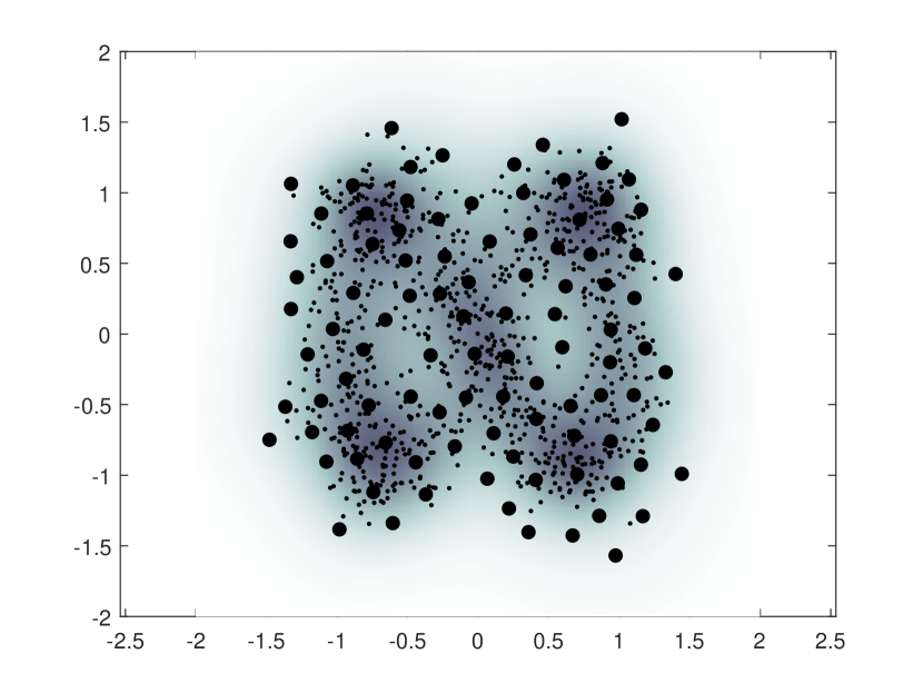
(a) The function $f(x)$ and landmarks $L$ on top of the data set $D$

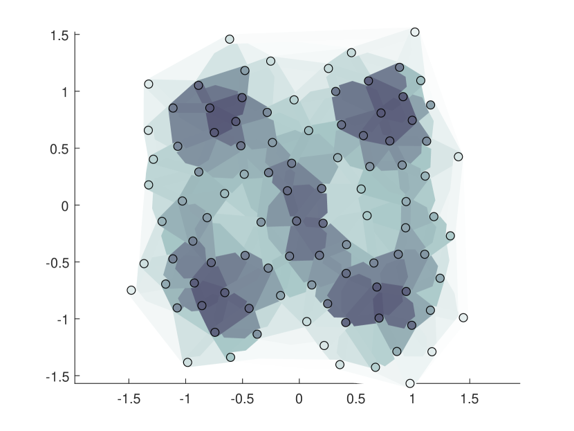
(b) The complex $X_{L}$, with persistence values indicated by shading

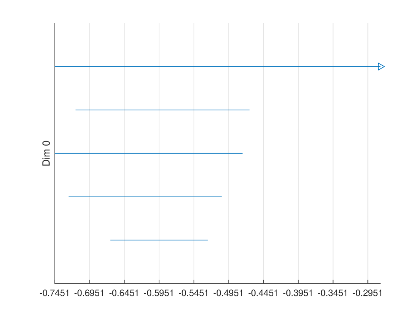
(c) $\beta_{0}$ diagram

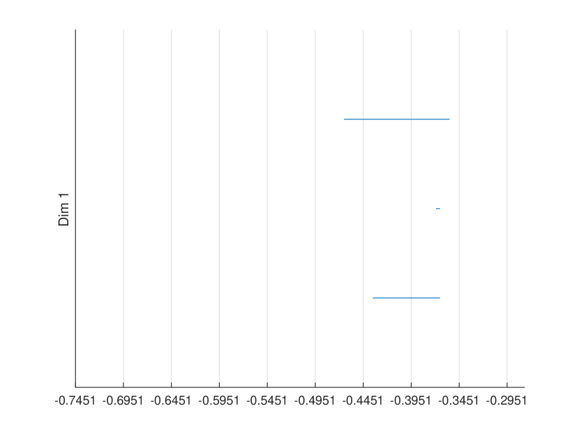
(d) $\beta_{1}$ diagram

Figure 2: The “infinity” data set from [19]. The function $f(z)=-\log(\rho(z))$ and landmark points $L$ are overlayed on the data set in Figure 2(a), and $X_{L}$ is shown in 2(b). The first two Javaplex persistence diagrams are shown in 2(c) and 2(d).

4.2 The continuous Ising model

Our second example illustrates a higher-dimensional persistence function which appears in statistical mechanics.

Let

$$X=\left\{\sigma\in\mathbb{R}^{d}:|\sigma_{i}|\leq 1\right\},$$

be the state space of the continuous form of the one-dimensional Ising model on $d$-sites, whose discrete form includes only the values $\sigma_{i}\in\{1,-1\}$. The values $\sigma_{i}$ are called the “spin” values. Let

$$H(\sigma)=-\sum_{i=1}^{d-1}\sigma_{i}\sigma_{i+1}$$

be the corresponding Hamiltonian function with no external field. We also consider the circular case, in which we add a $-\sigma_{n}\sigma_{1}$ term, corresponding to the Ising model on the circle. We define $f(\sigma)=H(\sigma)$ in either case. States with low values of $H(\sigma)$ tend to be ones in which neighboring points are similar. There are two global minimizers when all $\sigma_{i}$ are all simultaneously equal to $\pm 1$, in which case we have $H(\sigma)=-(d-1)$. At higher energy levels, one expects interesting homological features in the continuous limit, as the number of sites becomes large.

We selected landmarks point by selecting 20 distinct states with values $\sigma_{i}\in\{\pm 1\}$ among those with low energy values, and we computed the corresponding persistent homology groups $H_{k}^{a,b}(X_{L})$ for both the interval and and circle example. The persistence diagrams are shown in Figure 3, together with illustrations of the higher dimensional features.

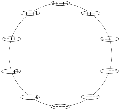
(a) A 1-cycle for the interval case

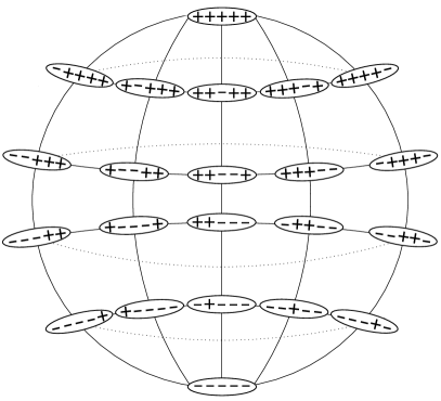
(b) A 2-cycle parametrized by the sphere

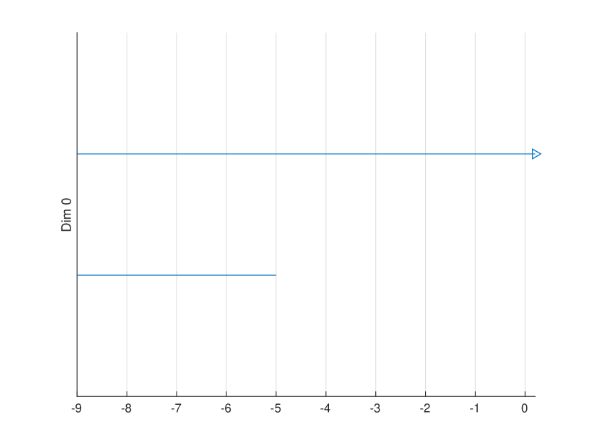
(c) $\beta_{0}$ diagram, circle

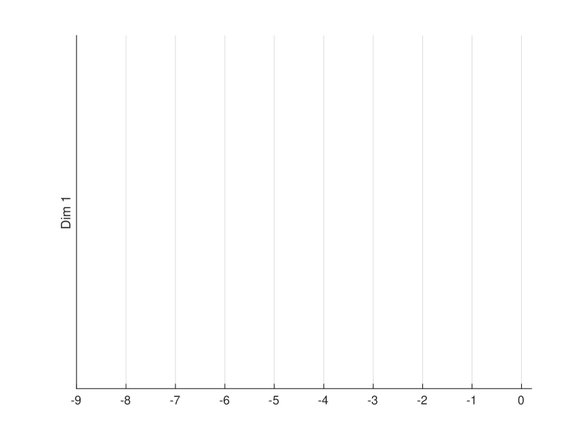
(d) $\beta_{1}$ diagram, circle

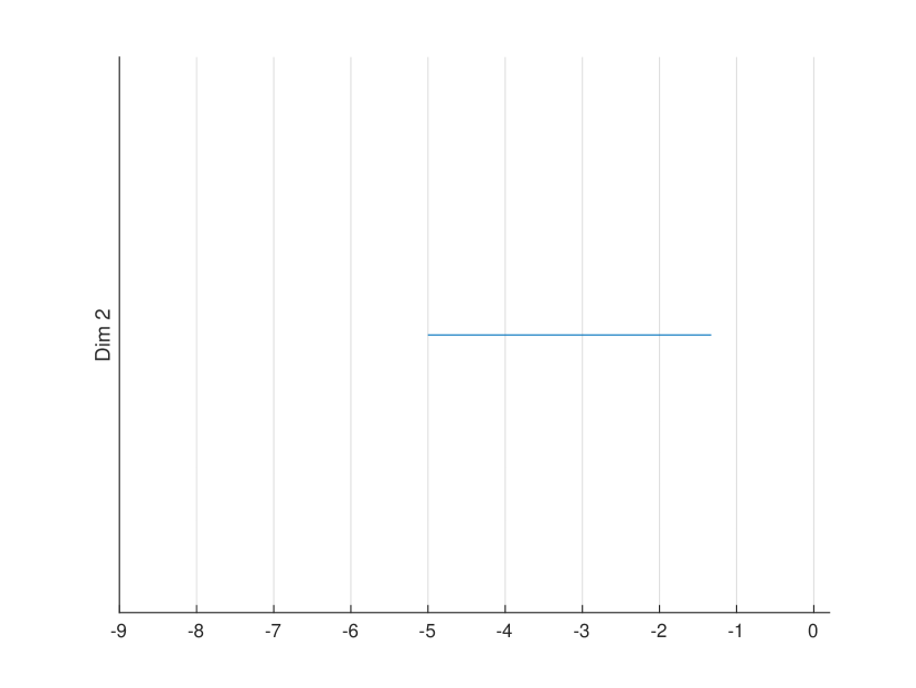
(e) $\beta_{2}$ diagram, circle

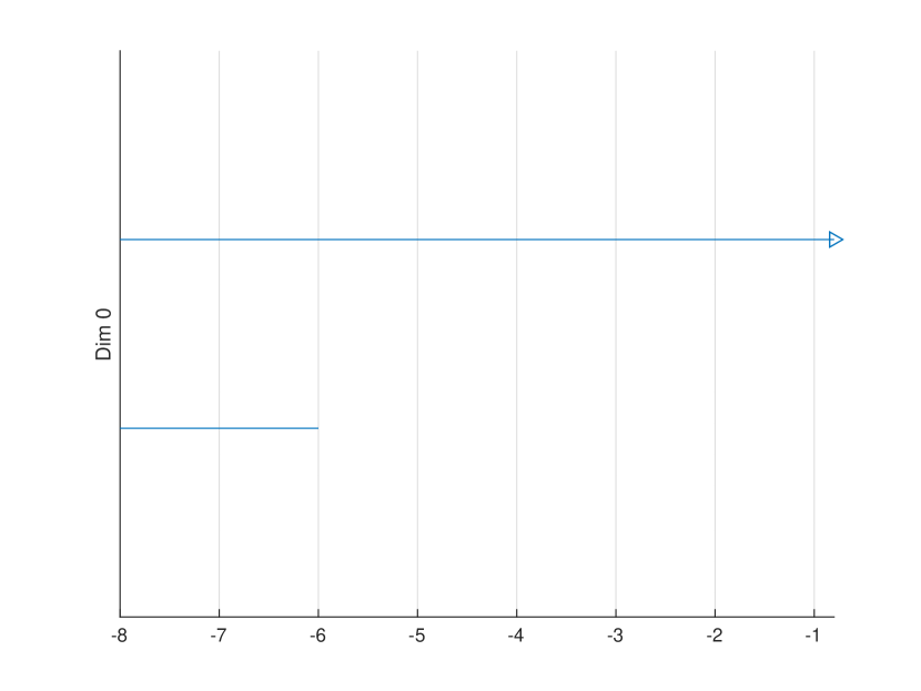
(f) $\beta_{0}$ diagram, interval

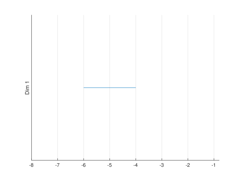
(g) $\beta_{1}$ diagram, interval

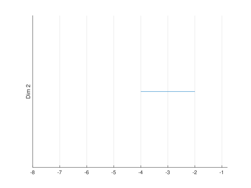
(h) $\beta_{2}$ diagram, interval

Figure 3: The top row shows representative 1- and 2-cycles for the two instances of the Ising model considered in this section (the interval and a circle, respectively). The middle and bottom rows show the for 9 sites on an circle (middle) and the interval (bottom). Each one has two $\beta_{0}$ features at lowest energy corresponding to all spin values being the same. The top row illustrates a nontrivial 1-cycle for the interval, and the nonzero $\beta_{2}$ feature that is present in both.

4.3 Configuration space

In the last example, we apply the complex to produce the Betti numbers of a topologically interesting space, by inventing a function whose local minimizers are the space.

Let $C_{n}$ be the configuration space of $n$ distinct ordered points $p_{i}\in\mathbb{R}^{2}$, in other words the complement of the diagonal in $(\mathbb{R}^{2})^{n}$. Then $C_{n}$ deformation retracts onto an $(n-1)$-dimensional singular subspace $C^{\prime}_{n}\subset C_{n}$ which sometimes appears in robotics, in which $(p_{1},...,p_{n})$ is mean-centered, and each $p_{i}$ is of distance exactly one to its nearest neighbor. For instance, a typical point in $C^{\prime}_{5}$ would be

where we have drawn a a dashed line between a point and its nearest neighbor. The homology $H_{k}(C^{\prime}_{n})\cong H_{k}(C_{n})$ space is well-known [9], and for $n=3$ the Betti numbers are given by $(\beta_{0},\beta_{1},\beta_{2})=(1,3,2)$.

(a) $\beta_{0}$ diagram

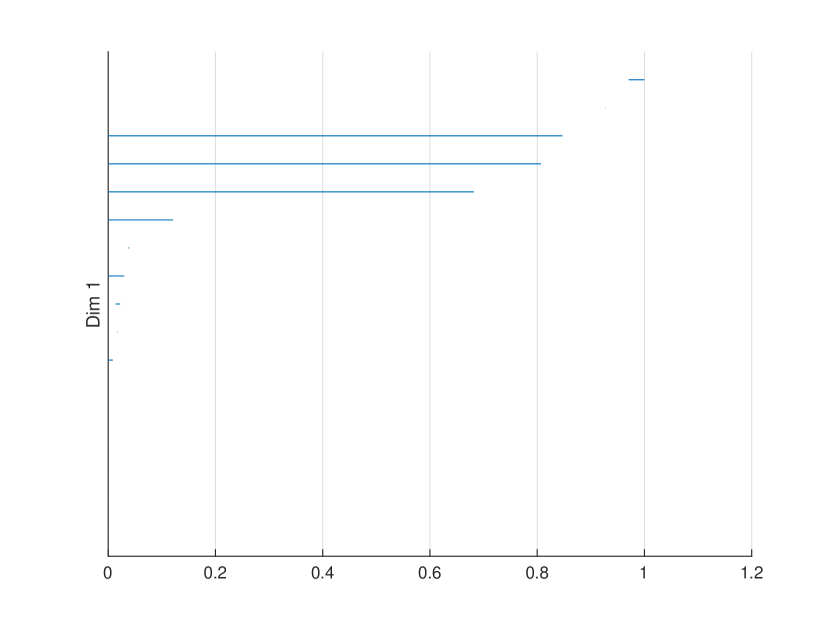
(b) $\beta_{1}$ diagram

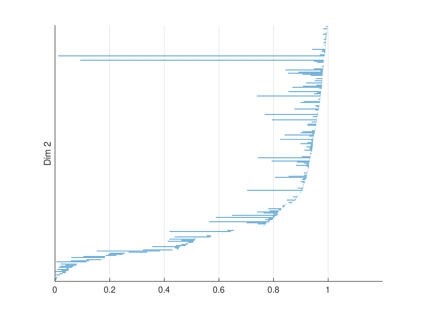
(c) $\beta_{2}$ diagram

Figure 4: Persistence diagrams for the function in (11) whose extremal points are the configuration space $C^{\prime}_{3}$. The three diagrams show the anticipated Betti numbers for this space, ending a little below the value $f(p_{1},p_{2},p_{3})=1$, which is the smallest value at which points may collide.

We then consider the following function, which has local minimizers at the points of $C^{\prime}_{3}$:

$$f(p_{1},p_{2},p_{3})=\max_{i}\left(\min_{j\neq i}\left(\lVert p_{i}-p_{j}\rVert^{2}-1\right)^{2}\right)$$ (11)

We then take

$$X=\{(p_{1},p_{2},p_{3})\in\mathbb{R}^{6}:p_{1}+p_{2}+p_{3}=(0,0)\},$$

so that the sublevel sets of $f$ are compact when taken as a function on $X=\mathbb{R}^{4}$. We sampled 100 landmark points which are maximally spread out in the range $f^{-1}(-\infty,.1]$ using the max of min distance algorithm. The persistence diagrams are shown in Figure 4.

References

- [1] Henry Adams and Michael Moy. Topology applied to machine learning: From global to local. Frontiers in Artificial Intelligence, 4:668302, 05 2021.
- [2] Kenes Beketayev, Damir Yeliussizov, Dmitriy Morozov, Gunther Weber, and Bernd Hamann. Measuring the error in approximating the sub-level set topology of sampled scalar data. International Journal of Computational Geometry and Applications, 28:57–77, 03 2018.
- [3] G. Carlsson. Topological pattern recognition for point cloud data*. Acta Numerica, 23:289 – 368, 2014.
- [4] Gunnar Carlsson. Topology and data. Bulletin of The American Mathematical Society, 46:255–308, 04 2009.
- [5] Gunnar Carlsson. Persistent homology and applied homotopy theory, chapter 8. CRC Press, 2019.
- [6] F. Chazal, L. Guibas, S. Oudot, and P. Skraba. Persistence-based clustering in riemannian manifolds. J. ACM, 60:41:1–41:38, 2013.
- [7] Yu-Min Chung, W. Cruse, and A. Lawson. A persistent homology approach to time series classification. ArXiv, abs/2003.06462, 2020.
- [8] Yu-Min Chung, Chuan-Shen Hu, Yu-Lun Lo, and Hau-Tieng Wu. A persistent homology approach to heart rate variability analysis with an application to sleep-wake classification. Frontiers in Physiology, 12:202, 2021.
- [9] F.R. Cohen. On configuration spaces, their homology, and lie algebras. Journal of Pure and Applied Algebra, 100(1):19–42, 1995.
- [10] Herbert Edelsbrunner and John Harer. Persistent homology—a survey. Discrete and Computational Geometry - DCG, 453, 01 2008.
- [11] David Günther, Jan Reininghaus, Hubert Wagner, and Ingrid Hotz. Efficient computation of 3d morse-smale complexes and persistent homology using discrete morse theory. The Visual Computer, 28:1–11, 10 2012.
- [12] Gurobi Optimization LLC. Gurobi optimizer reference manual, 2021.
- [13] J. Milnor, M. Spivak, and R. Wells. Morse Theory. (AM-51), Volume 51. Princeton University Press, 1969.
- [14] Joshua Mirth, Yanqin Zhai, Johnathan Bush, Enrique G. Alvarado, Howie Jordan, Mark Heim, Bala Krishnamoorthy, Markus Pflaum, Aurora Clark, Y Z, and Henry Adams. Representations of energy landscapes by sublevelset persistent homology: An example with n -alkanes. The Journal of Chemical Physics, 154(11), 2020.
- [15] Audun Myers, Firas Khasawneh, and Brittany Fasy. Separating persistent homology of noise from time series data using topological signal processing, 12 2020.
- [16] Ken-Ichi Nishikawa and Huzio Nakano. A continuous ising model exhibiting phase transitions of first or second order. Progress of Theoretical Physics, 56:773–785, 09 1976.
- [17] Jose Perea and John Harer. Sliding windows and persistence: An application of topological methods to signal analysis. Foundations of Computational Mathematics, 15, 07 2013.
- [18] Nalini Ravishanker and Renjie Chen. Topological data analysis (tda) for time series, 2019.
- [19] Nathaniel Saul and Chris Tralie. Scikit-tda: Topological data analysis for python, 2019. https://doi.org/10.5281/zenodo.253369.
- [20] Lee M. Seversky, S. Davis, and M. Berger. On time-series topological data analysis: New data and opportunities. 2016 IEEE Conference on Computer Vision and Pattern Recognition Workshops (CVPRW), pages 1014–1022, 2016.
- [21] Andrew Tausz, Mikael Vejdemo-Johansson, and Henry Adams. JavaPlex: A research software package for persistent (co)homology. In Han Hong and Chee Yap, editors, Proceedings of ICMS 2014, Lecture Notes in Computer Science 8592, pages 129–136, 2014. available at http://appliedtopology.github.io/javaplex.
- [22] Sarah Tymochko, Elizabeth Munch, Jason Dunion, Kristen Corbosiero, and Ryan Torn. Using persistent homology to quantify a diurnal cycle in hurricanes. Pattern Recognition Letters, 133:137–143, 2020.