MAHGIC: A Model Adapter for the Halo-Galaxy Inter-Connection

Abstract

We develop a model to establish the interconnection between galaxies and their dark matter halos. We use Principal Component Analysis (PCA) to reduce the dimensionality of both the mass assembly histories of halos/subhalos and the star formation histories of galaxies, and Gradient Boosted Decision Trees (GBDT) to transform halo/subhalo properties into galaxy properties. We use two sets of hydrodynamic simulations to motivate our model architecture and to train the transformation. We then apply the two sets of trained models to dark matter only (DMO) simulations to show that the transformation is reliable and statistically accurate. The model trained by a high-resolution hydrodynamic simulation, or by a set of such simulations implementing the same physics of galaxy formation, can thus be applied to large DMO simulations to make ‘mock’ copies of the hydrodynamic simulation. The model is both flexible and interpretable, which paves the way for future applications in which we will constrain the model using observations at different redshifts simultaneously and explore how galaxies form and evolve in dark matter halos empirically.

1 Introduction

In the framework of the $\Lambda$CDM cosmology, galaxies are assumed to form in dark matter halos produced by the gravitational instability of the cosmic density field (Mo et al., 2010; Wechsler & Tinker, 2018). A key step in understanding the formation and evolution of galaxies is, therefore, to establish and understand the interconnection between galaxies and dark matter halos. A variety of methods have been proposed and used to achieve this goal, such as: full numerical simulation that models subgrid physics numerically (e.g., Vogelsberger et al., 2014; Schaye et al., 2015; Crain et al., 2015; Nelson et al., 2019; Pillepich et al., 2018b; Springel et al., 2018; Nelson et al., 2018; Naiman et al., 2018; Marinacci et al., 2018), matching galaxies and halos based on abundance (Mo et al., 1999; Vale & Ostriker, 2004; Guo et al., 2010; Simha et al., 2012), clustering (Guo et al., 2016), and age (Hearin & Watson, 2013; Hearin et al., 2014; Meng et al., 2020), halo occupation distribution (Jing et al., 1998; Berlind & Weinberg, 2002), the conditional luminosity function (Yang et al., 2003) and conditional color-magnitude distribution (Xu et al., 2018), and empirical models based on the star formation histories of galaxies (Mutch et al., 2013; Lu et al., 2014, 2015; Moster et al., 2018; Behroozi et al., 2019; Moster et al., 2020). These methods have yielded important results about the halo-galaxy interconnection. However, some issues still remain in such modeling. First, to build a successful model requires a systematic selection of significant halo features as predictors of the galaxy properties. The features selected should be such that they can be modeled reliably, are adaptable to new observational data, are non-redundant and yet sufficient to describe the data. Second, to simplify the mapping from halos to galaxies needs some pre-processing of the input features to make the model easily interpretable. Finally, to suppress over-fitting of the data the model should be able to capture potential non-linearities in the halo-galaxy interconnection and should include an automated regularization. The deep neural network (e.g., He et al., 2016; Huang et al., 2017) provides a possible solution, but the structures of the networks need to be tuned and the physical interpretation underlying these structures is not straightforward.

Empirical models for the halo-galaxy relation in the literature can roughly be classified into two categories according to their architecture. Models in the first category, which may be called ‘transparent-box’ models, include those based on abundance matching, clustering and age matching, conditional luminosity function, conditional color-magnitude distribution, and parametric mapping between halo and galaxy properties. These models are directly motivated by physical considerations, hence can be interpreted easily. However, these models usually adopt a set of halo features that may not be optimal for predicting galaxy properties owing to the loss of information and the degeneracy of halo properties. Furthermore, for models with parametric mapping, the number of features is usually limited because of the difficulty in creating multi-variate parametric formulations. This limits the flexibility of the model. Models in the other category, which may be referred to as ‘black-box’ models, usually use complex non-linear mappings, such as deep neural networks, to link halos and galaxies. These models can in principle be designed and tuned to make precise predictions for a large set of object and field properties, such as the baryon fraction in halos (Sullivan et al., 2018), halo stellar and gas properties (Moster et al., 2020; Agarwal et al., 2018), galaxy images (Zanisi et al., 2021), and density fields (Horowitz et al., 2021; Wadekar et al., 2020). Their major problem is that the complexity of the model can significantly hinder the interpretability.

The gap between the ‘transparent-box’ and ‘black-box’ models motivates us to develop a scheme that takes advantages of both categories in their interpretability and flexibility. This can be achieved by using a deep neural network, pruning its overly complicated parts, and replacing its mandatory parts with sub-models that have clearer physical interpretations. Since more pruning and replacing in general makes a model more transparent but less flexible, the pruning and replacing steps can be made adjustable, so that the model is an adapter that allows a continuous transition between physically-motivated models and those based on modern deep learning.

To modify a deep neural network for our purpose, we can decompose the network into three parts along the information flow. The first, which can be viewed as a feature extractor, is a set of layers that transforms the input of physical variables into a set of reduced hidden variables to simplify the regression problem. The second, called the regressor, consists of set of layers that maps the hidden input into a hidden output. The last part, which can be viewed as a feature restorer, is a set of layers that restores physical quantities from the hidden output of the regressor. Thus, the key to building our desired adapter is to prune and replace the three parts to make them interpretable.

In a recent paper, Chen et al. (2021, thereafter, Paper-I) developed an empirical method to link dark matter halos to central galaxies that form within them. They adopted a linear dimension reduction technique based on Principal Component Analysis (PCA) and a tree-based model ensemble technique called Gradient Boosted Decision Trees (GBDT) to establish the halo-galaxy interconnection. This method has the following advantages. First, by applying the GBDT regressors to simulated halos and galaxies, one can identify key halo properties that are the most relevant to the stellar properties of galaxies. This clearly demonstrates that the input features of an empirical model should be properly designed to avoid irrelevant and redundant halo properties. Second, by using PCA, the mass assembly history (MAH) of a dark matter halo, which in general is complex, can be described by a small number of principal components (PCs) without much information loss. As demonstrated in Paper-I and Chen et al. (2020), PCs of subhalo MAH are not only tightly correlated with halo structural and environmental properties, but are also the most important quantities to predict the variance of the star-forming main sequence. Similar techniques were used to reduce the dimensionality of halo MAH and find the principal direction in the halo property space (e.g. Jeeson-Daniel et al., 2011; Wong & Taylor, 2012), and to approximate the SFH of galaxies and find the principal direction in the galaxy color space (e.g. Cohn & van de Voort, 2015; Cohn, 2018; Chaves-Montero & Hearin, 2020, 2021). Finally, the use of GBDT regressors and classifiers can capture non-linear relations between halos and galaxies without introducing significant over-fitting. The GBDT contains the non-linearity of the whole model in a single layer, making the model easily interpretable. All these advantages are important to take into account when modeling the halo-galaxy interconnection. In the model presented here, we therefore adopt PCA and GBDT for the pruning and replacing steps, respectively.

The interpretability of the model allows one to use both hydrodynamic simulations and observations to motivate and train the model. Depending on the training set, the model can be applied in two different ways. First, if the model is trained by a hydrodynamic simulation, or by a set of simulations implementing the same set of physical processes, one can apply it to another, generally much larger, dark-matter-only (DMO) simulation to generate a copy using the dark matter halo population in the DMO simulation. This is an important application, because full hydrodynamic simulations are usually run with relatively small box size. Such simulations may be sufficient to model galaxy formation in individual halos, but may not be able to provide a fair sample of the universe owing to the cosmic variance associated with the small simulation volume (see, e.g., Somerville et al., 2004; Moster et al., 2011; Chen et al., 2019; Meng et al., 2020). The copy made by the trained model combines the advantages of these two types of simulations, producing a much larger sample statistically equivalent to the training set but with a much reduced cosmic variance. Second, if observational data are used to constrain the model, the architecture learned from hydrodynamic simulations can be used for the model design, so that model parameters inferred from observations can be interpreted in terms of physical processes. For example, the mapping from halos to galaxies obtained from observational data can be used to reveal halo properties that are the most important in determining a given set of properties of the galaxy population. The model inferred from the data can also be compared directly with that trained by the hydrodynamic simulation to test the assumptions made in the simulation. Another potential application, which is beyond the scope of this paper, is to use the constrained halo-galaxy relation (the constrained galaxy bias model) to populate large-box simulations to test precision cosmology.

In this paper, we adopt the above adapter architecture and extend the model described in Paper-I for central galaxies to a full pipeline for the whole galaxy population. The pipeline, named MAHGIC- a Model Adapter for the Halo-Galaxy Inter-Connection, is trained and tested here using hydrodynamic simulations, before we apply it to observational data in the future. The paper is organized as follows. In §2 we introduce the numerical simulations, the halo properties, and the samples used in our analysis. In §3, we describe our model and how the different components of the model are pieced together into the pipeline MAHGIC. We test the performance of the pipeline in §4 using hydrodynamic simulations. Our main results are summarized and discussed in §5.

Table 1: Summary of the four simulations used in this paper. Listed information includes cosmological parameters, box size $L_{\rm box}$, number of resolution units $N_{\rm resolution}$, dark matter particle mass $m_{\rm dark\ matter}$, and target baryon mass $m_{\rm baryon}$. Cosmologies are taken from Planck15 (Ade et al., 2016), WMAP5 (Dunkley et al., 2009), and Planck13 (Ade et al., 2014). In TNG, $N_{\rm resolution}$ is the number of dark matter particles plus the initial number of gas cells, and gas cells are refined or de-refined such that their mass is kept within a factor of 2 of $m_{\rm baryon}$. In EAGLE, $N_{\rm resolution}$ is the number of dark matter particles plus the initial number of baryonic particles and $m_{\rm baryon}$ is the initial baryonic particle mass. In TNG-Dark and ELUCID, $N_{\rm resolution}$ is the number of dark matter particles.

Simulation	Cosmology	$L_{\rm box}$ $[\,h^{-1}{\rm{cMpc}}]$	$N_{\rm resolution}$	$m_{\rm dark\ matter}$ $[\,h^{-1}{\rm M_{\odot}}]$	$m_{\rm baryon}$ $[\,h^{-1}{\rm M_{\odot}}]$
TNG	Planck15: $h=0.6774$, $\Omega_{\Lambda,0}=0.6911$, $\Omega_{M,0}=0.3089$, $\Omega_{B,0}=0.0486$, $\Omega_{K,0}=0$, $\sigma_{8}=0.8159$, $n_{s}=0.9667$	75	$2\times 1820^{3}$	$5.1\times 10^{6}$	$9.4\times 10^{5}$
TNG-Dark			$1820^{3}$	$6.0\times 10^{6}$	-
ELUCID	WMAP5: $h=0.72$, $\Omega_{\Lambda,0}=0.742$, $\Omega_{M,0}=0.258$, $\Omega_{B,0}=0.044$, $\Omega_{K,0}=0$, $\sigma_{8}=0.80$, $n_{s}=0.96$	$500$	$3072^{3}$	$3.08\times 10^{8}$	-
EAGLE	Planck13: $h=0.6777$, $\Omega_{\Lambda,0}=0.693$, $\Omega_{M,0}=0.307$, $\Omega_{B,0}=0.04825$, $\Omega_{K,0}=0$, $\sigma_{8}=0.8288$, $n_{s}=0.9611$	$67.8$	$2\times 1504^{3}$	$6.57\times 10^{6}$	$1.23\times 10^{6}$

2 The Data

2.1 The Simulations

Throughout this paper, we use four simulations to motivate, build, train, and test our pipeline, MAHGIC.

The first is Illustris-TNG (Nelson et al., 2019; Pillepich et al., 2018b; Springel et al., 2018; Nelson et al., 2018; Naiman et al., 2018; Marinacci et al., 2018), a suite of cosmological hydrodynamic simulations carried out with the moving mesh code Arepo (Springel, 2010). Processes for galaxy formation, such as gas cooling, star formation, stellar feedback, metal enrichment, and AGN feedback, are simulated with subgrid prescriptions tuned to match a set of observational data (see Weinberger et al., 2017; Pillepich et al., 2018a). A total of 100 snapshots, from redshift $z=20.0$ to $0$, are saved for each run. Halos are identified with the friends-of-friends (FoF) algorithm (Davis et al., 1985) with a linking length of $0.2$, and subhalos are identified with the Subfind algorithm (Springel et al., 2001; Dolag et al., 2009). Subhalo merger trees are constructed using the SubLink algorithm (Rodriguez-Gomez et al., 2015). To achieve a balance between sample size and resolution, we use the TNG100-1 run (thereafter TNG).

The second is TNG100-1-Dark, the DMO counterpart of TNG (thereafter TNG-Dark). It is run with the same cosmological parameters, box size, initial conditions, output snapshots as the hydrodynamic run, and it has mass and spatial resolutions similar to TNG.

The third is ELUCID (Wang et al., 2016), a DMO simulation obtained using the N-body code L-GADGET, a memory optimized version of GADGET-2 (Springel, 2005). A total of 100 snapshots, from redshift $z=18.4$ to $0$, are saved. Halos, subhalos and subhalo merger trees are identified and constructed using the same algorithms as TNG.

The final one is EAGLE (Schaye et al., 2015; Crain et al., 2015; McAlpine et al., 2016; The EAGLE team, 2017), a suite of cosmological hydrodynamic simulations run with the GADGET-3 tree-SPH code, an extension of GADGET-2 Springel (2005). A total of 29 snapshots, from $z=20$ to $0$, are saved. Halos and subhalos are identified by the same algorithms as TNG. Subhalo merger trees are constructed by the D-Trees algorithm (Jiang et al., 2014). We use the high-resolution run, EAGLE Ref-L0100N1504 (thereafter EAGLE) for our analysis, which has a resolution comparable to TNG.

The cosmology and simulation parameters of all the four simulations are listed in Table 1.

2.2 Subhalo Properties

The subhalo catalogs of both TNG and EAGLE present a variety of quantities, such as stellar mass, halo mass and star formation rate. The subhalo catalog of ELUCID gives the properties of of dark matter halos. As demonstrated by Chen et al. (2020), halo properties themselves have significant degeneracy, so that it is not necessary to include all halo properties in an empirical model. Furthermore, as demonstrated in Paper-I, galaxy stellar properties depend significantly only on a subset of all the halo properties. Motivated by the results of these two papers, we choose to use the following set of subhalo properties that are the most relevant to the halo-galaxy interconnection.

• $M_{\rm h}$: the ‘top-hat’ mass of the host FoF halo of a subhalo. This halo mass is calculated within a virial radius within which the overdensity is equal to that given by the spherical collapse model (Bryan & Norman, 1998). The corresponding virial radius and virial velocity are denoted as $R_{\rm h}$ and $V_{\rm h}$, respectively.

• $j_{\rm infall}$: the normalized orbital angular momentum of a satellite subhalo, defined as

  $$j_{\rm infall}=\frac{\|\Delta{\bf r}\times\Delta{\bf v}\|}{\sqrt{2}R_{\rm h,cent}V_{\rm h,cent}},$$ (1)

  where $\Delta{\bf r}$ and $\Delta{\bf v}$ are the position and velocity of the satellite relative to its central subhalo, respectively, and $R_{\rm h,cent}$ and $V_{\rm h,cent}$ are the virial radius and virial velocity of the central subhalo, respectively . $j_{\rm infall}$ is defined for a satellite subhalo at the infall time.

• $\tau_{\rm merge}$: the merger time of a satellite subhalo, defined as

  $$\tau_{\rm merge}=\log\frac{1+z_{\rm merge}}{1+z_{\rm infall}},$$ (2)

  where $z_{\rm merge}$ is the redshift just before the satellite merges into the central subhalo, and $z_{\rm infall}$ is the redshift when the satellite falls into the host FoF halo.

• $I_{\rm merge}$: a binary indicator to describe whether or not a subhalo has merged by $z=0$. If it has merged, $I_{\rm merge}=1$; otherwise $I_{\rm merge}=0$. Note that $\tau_{\rm merge}$ is undefined for satellites that have not yet merged by $z=0$. $I_{\rm merge}$ is defined to include such satellites in our model (§3.3).

• $M_{*}$: the stellar mass of a subhalo. This is defined as the mass within twice the stellar half mass radius for TNG, and within $30$ physical kpc for EAGLE.

• $\rm SFR$: the star formation rate within the same radius as that for $M_{*}$.

• $M_{\rm*,int}$: the total stellar mass ever formed in the history of a subhalo: $\sum_{n}{\rm SFR}_{n}\Delta t_{n}$, where ${\rm SFR}_{n}$ is the SFR at $n$th snapshot in the history and $\Delta t_{n}$ is the time interval spanned by the snapshot. $M_{\rm*,int}$ will be the direct output of our model in §3. It is different from $M_{*}$ in that the mass loss due to stellar evolution and mass changes due to mergers are not taken into account. Merger-triggered changes in the SFR are included in $M_{\rm*,int}$. When comparing with observations, these effects should be included by properly assuming a stellar evolution model, an initial mass function (e.g., Salpeter, 1955; Chabrier, 2003; Zhou et al., 2019), and a merger model. Our test using the TNG simulation shows that the simple addition of $M_{\rm*,int}$, of a galaxy with all the progenitors merged into it, is $\sim 0.3\ {\rm dex}$ larger than $M_{*}$ at all redshifts for $M_{*}>10^{8}\,h^{-1}{\rm M_{\odot}}$.

• sSFR: the specific star formation rate, defined as ${\rm sSFR}={\rm SFR}/M_{\rm*,int}$.

Note that $M_{*}$, SFR, $M_{\rm*,int}$ and sSFR are defined only in the hydrodynamic simulations, TNG and EAGLE. Other properties are defined also in TNG-Dark and ELUCID.

As shown in Paper-I, the halo-galaxy connection depends not only on the current status of a halo, but also on its assembly history. Following Paper-I, we define the subhalo mass assembly history (MAH), ${\bf M}_{\rm h}$, for a central subhalo as the set of $M_{\rm h}$ values in the main branch of the subhalo merger tree rooted in this subhalo. We also define the star formation history (SFH), ${\bf M}_{\rm*,int}$, of a galaxy as the set of $M_{\rm*,int}$ values in the main branch of the subhalo merger tree rooted in the host subhalo of the galaxy.

The discrete forms of the MAH and the SFH in general are each a ‘vector’ (tuple) in high-dimensional configuration space, and the information contained in these vectors may be highly degenerate. To extract useful information from them, some method of dimension reduction is needed. Here we follow Paper-I (see its Appendix A for a detailed description) to reduce the dimensionality of the MAH and the SFH by PCA whenever it is needed. The application of PCA to a MAH (or a SFH) reduces it to a set of PCs, with the first several expected to be capable of capturing its main properties. We denote the PCs of the MAH and SFH as ${\bf pc}_{\rm h}$ and ${\bf pc}_{*}$, respectively. The details of the related analyses are described in §3.

2.3 Tree Decomposition and Subhalo Samples

To reduce the complexity of the empirical model, we do not attempt to model the stellar content for each single subhalo. Instead, we decompose each subhalo merger tree into a set of disjoint branches, $\{b\}$, each of which is a chain of subhalos that form the main branch of a root subhalo. The decomposition is processed through the following steps:

• Starting from the root subhalo $h_{r}$ of the whole subhalo merger tree (i.e., the subhalo that does not have any descendant), we use all subhalos in the main branch of $h_{r}$ to form a single branch $b$.

• Subhalos attached to $b$ are removed from the tree, resulting in a set of sub-trees of the original tree.

• Treating each sub-tree as a new ‘tree’, we recursively perform the same decomposition for all the sub-trees until all subhalos in the original tree are assigned into branches. All the branches collectively form $\{b\}$.

For each branch, we walk through it from high to low redshift. We define the infall redshift $z_{\rm infall}$ of the branch as the redshift of the last snapshot when the subhalo is still a central subhalo. We define the infall halo mass $M_{\rm h,infall}$ as the halo mass at $z_{\rm infall}$. Note that this definition is valid for branches in both sub-trees and the original tree.

To achieve a balance of numerical stability and sample size, we select all branches with $M_{\rm h,infall}>M_{\rm h,limit}=10^{11}\,h^{-1}{\rm M_{\odot}}$. The subhalos in the selected branches are the main sample we use in our model and analysis. Such a selection ensures that galaxies are well resolved in TNG and EAGLE, and that the sample size is still sufficiently large to allow for model learning and testing. We have checked that our model is stable when using a lower mass limit. To alleviate computational cost, we apply and test our model using a sub-box with $200\,h^{-1}{\rm{Mpc}}$ side-length from ELUCID. As shown in Appendix A and Figure 12, this sub-box can already significantly reduce the cosmic variance in comparison with TNG and EAGLE, and is thus sufficient for our purpose.

The above mass limit is suitable for TNG, TNG-Dark and EAGLE, but is too small for ELUCID. The lowest halo mass that can be resolved by ELUCID is $\sim 6\times 10^{9}\,h^{-1}{\rm M_{\odot}}$, about $50\times$ larger than that in the other three simulations. Because of this, the ELUCID simulation cannot trace the MAH of a subhalo to sufficiently high redshift when the star formation in the branch is already significant. To overcome this limitation, we use merger trees from TNG-Dark to extend all branches in ELUCID down to the same mass limit. For each branch in ELUCID, we pick a branch in TNG-Dark at the same $z_{\rm infall}$ and with the same $M_{\rm h,infall}$. The missed part of MAH in ELUCID at high redshift is extended by this picked branch, with proper interpolation to adjust the redshift sampling. Note that this is different from Chen et al. (2019) where analytical halo merger trees obtained from a Monte Carlo (MC) implementation were used to extend the MAH. Our choice is motivated by the fact that the merger trees from high-resolution simulations are more precise, and are usually used to calibrate the analytical trees. As shown in Appendix A, the extended MAHs of ELUCID match well with those obtained from the other three simulations. Any branch that terminates before it reaches the upper redshift limit (set by the redshift of the first snapshot) is padded with a small value for numerical stability.

3 The Empirical Model

3.1 Overall Design Strategies

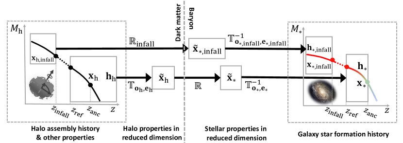
Figure 1: The pipeline of the model MAHGIC. The model separately deals with central (lower channel in the figure) and satellite galaxies (upper channel). Galaxy properties at the anchor redshift, ${\bf x}_{*}$, and galaxy SFH in the central stage, ${\bf h}_{*}$, are mapped from subhalo MAH ${\bf h}_{\rm h}$, and other halo properties at the anchor redshift, ${\bf x}_{\rm h}$. Three transformations $(\mathbb{T}_{{\bf o}_{\rm h},{\bf e}_{\rm h}},\mathbb{R},\mathbb{T}_{{\bf o}_{*},{\bf e}_{*}})$ are trained and applied for the central stage. Galaxy properties at the infall time, ${\bf x}_{\rm*,infall}$, and galaxy SFH in the satellite stage, ${\bf h}_{\rm*,infall}$, are mapped from halo properties at the infall time, ${\bf x}_{\rm h,infall}$. Two transformations $(\mathbb{R}_{\rm infall},\mathbb{T}_{{\bf o}_{\rm*,infall},{\bf e}_{\rm*,infall}})$ are trained and applied to the satellite stage. The whole pipeline consists of multiple redshift pieces, one of which is shown here.

Table 2: Notations for variables and transformations used by MAHGIC. Notations for central galaxies are listed here, while those for satellite galaxies can be obtained by adding a subscript ‘infall’ (e.g., ${\bf x}_{\rm h,infall}$ for the properties of satellite subhalo at infall time). The order of the listed notations follows the pipeline in the application phase (see §3), which is consistent with information flow in Figure 1.

Variables	Explanation
$({\bf x}_{\rm h},{\bf h}_{\rm h})$	Physical properties of subhalo. ${\bf x}_{\rm h}$ are subhalo properties at the anchor redshift $z_{\rm anc}$ of the tree branch. ${\bf h}_{\rm h}$ is the MAH of this branch.
${\bf\tilde{x}}_{\rm h}$	Subhalo properties in the space of reduced dimension, including ${\bf x}_{\rm h}$ and a set of PCs of subhalo MAH. It is connected to the physical subhalo properties through the representation transformation of subhalo, ${\bf\tilde{x}}_{\rm h}=\mathbb{T}_{{\bf o}_{\rm h},{\bf e}_{\rm h}}({\bf x}_{\rm h},{\bf h}_{\rm h})$.
${\bf\tilde{x}}_{*}$	Galaxy properties in the space of reduced dimension, including ${\bf x}_{*}$ and a set of PCs of galaxy SFH. It is produced through the halo-galaxy mapping, ${\bf\tilde{x}}_{*}=\mathbb{R}({\bf\tilde{x}}_{\rm h})$.
$({\bf x}_{*},{\bf h}_{*})$	Physical properties of galaxy. ${\bf x}_{*}$ are galaxy properties at $z_{\rm anc}$. ${\bf h}_{*}$ is the SFH of galaxies in this branch. They are produced through the inverse of the representation transformation of galaxy, $({\bf x}_{*},{\bf h}_{*})=\mathbb{T}^{-1}_{{\bf o}_{*},{\bf e}_{*}}({\bf\tilde{x}}_{*})$.

As discussed in §1, the goal of MAHGIC is to first use hydrodynamic simulations to motivate and train our model design, and then to apply it to DMO simulations. Motivated by the results obtained in Chen et al. (2020) and Paper-I, we adopt the following strategies to construct the model:

1. Central and satellite galaxies are modeled separately. This is motivated by the fact that processes regulating star formation are very different for the two populations. For example, a satellite galaxy after infall may undergo significant environmental quenching due to tidal stripping and ram-pressure stripping, which may be less important for a central galaxy. Such a separation is commonly adopted in other empirical models (e.g., Yang et al., 2012; Mutch et al., 2013; Lu et al., 2014, 2015; Hearin et al., 2016; Moster et al., 2018; Behroozi et al., 2019).

2. Halo properties used in the model are required to be robust. They should be insensitive to baryonic effects and stable against changes in numerical resolution. This is required by our goal, as we want to train our model using hydrodynamic simulations, which contain baryonic effects and usually have a high resolution, and apply it to large DMO simulations where the baryonic effects are absent and the numerical resolution may be different. To reduce the impact of baryonic and resolution effects, we use the assembly history represented by halo mass $M_{\rm h}(z)$ as the main predictor of stellar properties, and avoid using the assembly history represented by the maximum circular velocity, $v_{\rm max}(z)$, which is sensitive to both effects. For the model of satellite galaxies, we use halo properties at the infall time as predictors, and avoid halo properties after the infall. As tested by us using TNG and ELUCID simulations, halo properties after infall are sensitive to baryonic effects and numerical resolution, while quantities defined at the infall time are stable (see Appendix A). Due to limited resolutions, large-volume DMO simulations like ELUCID in general are incapable of fully tracing the mass assembly history (MAH) of a halo to high redshift when its main progenitor becomes too small to be resolved. For such cases, we use the method described in §2.3 to extend the MAH down to a sufficiently low mass limit.

3. The model must be able to capture potential non-linearities in the halo-galaxy interconnection. We, therefore, build a deep model with multiple layers including representation, halo-galaxy mapping, and reconstruction. This mimics modern deep neural networks, where input values are first transformed to a simple representation and then fed into a traditional regressor or classifier to produce the output.

4. The model must be interpretable. This is needed because we want to understand the physics underlying the model, rather than just building a ‘black-box’ model. We achieve this by using interpretable prescriptions in all the layers of the model and we optimize them separately, an approach similar to the greedy algorithm in algorithm-design (e.g. Cormen et al., 2009; Sedgewick & Wayne, 2011). To be specific, in the representation and reconstruction layers, we use PCA to reduce the dimensionality of the subhalo MAH and the galaxy SFH. PCA is a simple and yet powerful dimension-reduction technique with robust mathematical interpretability. As demonstrated by Chen et al. (2020), the principal components (PCs) of subhalo MAH carry sufficient information about how halos form and are also strongly correlated with other halo structural and environmental properties. In addition, as demonstrated in Paper-I, these PCs are strongly correlated with galaxy SFH, thus providing an ideal way to do the halo-galaxy mapping. In the layer of halo-galaxy mapping, we adopt decision tree classifiers and regressors to map halo properties to galaxy stellar properties. Tree-based models are non-linear, so they are capable of dealing with potential non-linearities in the model. Trees are also interpretable through the importance values $\mathcal{I}(x)$ of individual predictors and the $R^{2}$ value of model performance (see Paper-I). Finally, the predicted stellar properties are used in the reconstruction layer to obtain the physical SFH.

5. The model should be flexible enough to accommodate constraints from current and future observations, and yet avoid over-fitting. In the context of Bayesian inference, model complexities can be increased to capture more subtle processes as more observational constraints become available. For the problem of galaxy formation concerned here, constraints are obtained from observations of galaxies at different redshifts. Thus, it is not useful to build a mapping that is valid only at a given redshift. Instead, we should construct the mapping on the basis of MAH and SFH. To do this, we use tree branches of MAH and SFH described in §2.3 as individual entries, and build a mapping of the PCs between the MAH and SFH branches. This has the advantage of avoiding an over-complicated model. We use GBDT in the halo-galaxy mapping to suppress over-fitting, as described in detail in Paper-I (see its Appendix B). As the amount of constraining data increases, one can use more PCs and more halo quantities as input features to accommodate the additional constraints.

To improve the accuracy of our model, we need to break the modeling into multiple pieces in redshift. The reasons for this are the following. First, the prediction of stellar properties is the most precise at the redshift where predictor halo properties are used. Indeed, as shown in Paper-I, $M_{\rm*,int}$ at a given redshift is predominantly determined by $M_{\rm h}$ at the redshift. The extension of the SFH towards higher redshift in general introduces cumulative errors, even if PCs are used, because the predictions of stellar PCs themselves contain error, as seen from Figure 2. Second, branches of different $z_{\rm infall}$ have different lengths in redshift coverage. To make the PCA feasible, we need to align the branches so that that they have the same length (see §3.2 and §3.3). If only one piece is used, artificial continuations are needed for MAHs that have different lengths, which can introduce artifacts and should be avoided.

Using multiple pieces is an analog to a non-parametric approach: it solves the problem at the expense of the interpretability. However, our model can avoid problems in a full non-parametric approach by using PCs for each of the pieces. In principle, the number of pieces and the locations of the breaking redshift can both be set as free hyperparameters and adjusted by an independent cross-validation process, depending on the quality of the training data and the form of the objective function. This is similar to a neural network, where neurons in the same layer are responsible for different regions of the feature space and should be adjusted according to the training data.

Taking account of all these requirements, we intend to build a deep interpretable model for galaxy formation in dark matter halos. The details are described in the following sections separately for central galaxies (§3.2) and satellite galaxies (§3.3). Figure 1 shows the outline of the model, and Table 2 lists the variables and transformations involved.

3.2 The Model for Central Galaxies

Our model for central galaxies follows closely that of Paper-I, with some modifications. In Paper-I we only modeled galaxies that are centrals at $z=0$ ($z_{\rm infall}=0$ according to our notation in this paper). Here we extend the modeling to include subhalo branches with all $z_{\rm infall}$. The procedures of our model are slightly different between the training phase and the application phase. For the training, we have information about both subhalos and galaxies, while for the application only subhalo properties are accessible. We describe the modeling in the training phase first, and then highlight the changes in the application phase.

Training phase. The goal of our model for central galaxies is to populate each branch with galaxies for all subhalos in the branch at $z\geq z_{\rm infall}$. Because the halo-galaxy relation is expected to change with redshift, we break the whole redshift range into $N_{\rm piece}$ pieces with separation redshift at $(z_{0},z_{1},z_{2},...,z_{N_{\rm piece}})$, where $z_{0}=0$ and $z_{N_{\rm piece}}$ is chosen to be sufficiently high to cover the desired redshift range. The model is built independently for each piece, with the $i$th piece responsible for all central galaxies in the redshift interval $(z_{i-1},z_{i}]$. For the sake of description, we refer to $z_{i-1}$ as the reference redshift and denote it as $z_{\rm ref}$; and to $z_{\rm i}$ as the anchor redshift and denote it as $z_{\rm anc}$. The relevance of these two redshifts to our description will become clear later in this section.

To model the $i$th piece, we select a reference sample, ${\rm S}_{\rm ref}$, which is defined as all tree branches with $z_{\rm infall}=z_{\rm ref}$. For each branch in ${\rm S}_{\rm ref}$, the subhalo MAH at $z<z_{\rm infall}$ is cut out, and the remaining MAH is denoted as $\bf{h}_{\rm h}$, which is a vector representing the values of $M_{\rm h}$ for all subhalos in this branch. We also take a set of halo properties at $z=z_{\rm anc}$, and denote them as ${\bf x}_{\rm h}$. We normalize ${\bf h}_{h}$ as

$${\bf\tilde{h}}_{\rm h}=\log\frac{{\bf h}_{\rm h}}{M_{{\rm h},z=z_{\rm anc}}},$$ (3)

and we apply PCA to ${\bf\tilde{h}}_{\rm h}$ to obtain a set of PCs, ${\bf pc}_{\rm h}$, a mean MAH ${\bf o}_{\rm h}$, and a set of eigen modes ${\bf e}_{\rm h}$. These PCs are combined with the set of halo properties, ${\bf x}_{\rm h}$, to form the vector ${\bf\tilde{x}}_{\rm h}=({\bf x}_{\rm h},{\bf pc}_{\rm h})$. This vector is the output of the representation layer, and is to be fed into the halo-galaxy mapping layer.

In this paper, we use $M_{\rm h}$ as the only properties at $z_{\rm anc}$, i.e., ${\bf x}_{\rm h}=(\log M_{{\rm h},z=z_{\rm anc}})$. As shown in Paper-I, the halo mass at a given redshift is the dominating factor in determining the stellar properties of the central galaxy hosted by the halo at the same redshift. For the output of the PCA, we follow Paper-I and use the first two PCs. More quantities and PCs can be added into ${\bf\tilde{x}}_{\rm h}$ when needed.

After the construction of ${\rm S}_{\rm ref}$ and the PCA template $({\bf o}_{\rm h},{\bf e}_{\rm h})$, we select all the remaining branches with $z_{\rm infall}\leqslant z_{\rm anc}$ that are not included in the reference sample. For any of these branches, if $z_{\rm infall}<z_{\rm ref}$, subhalos with $z<z_{\rm ref}$ are cut out from the branch. Otherwise, if $z_{\rm infall}>z_{\rm ref}$, satellite subhalos with $z<z_{\rm infall}$ are cut out, and the missed history between $z_{\rm ref}$ and $z_{\rm infall}$ is completed using the mean assembly rate of the reference sample scaled by the halo mass at $z_{\rm infall}$. With the trimming and completion, all MAHs in the remaining sample are vectors of the same length. They are then normalized and transformed by the PCA template $({\bf o}_{\rm h},{\bf e}_{\rm h})$ obtained from ${\rm S}_{\rm ref}$ to yield ${\bf\tilde{x}}_{\rm h}$ for these branches. The whole process of representation transformation from $({\bf x}_{\rm h},{\bf h}_{\rm h})$ to ${\bf\tilde{x}}_{\rm h}$ is denoted as $\mathbb{T}_{{\bf o}_{\rm h},{\bf e}_{\rm h}}$, and we write

$${\bf\tilde{x}}_{\rm h}=\mathbb{T}_{{\bf o}_{\rm h},{\bf e}_{\rm h}}({\bf x}_{\rm h},{\bf h}_{\rm h}).$$ (4)

We use the same technique to build the representation of the galaxy SFH in reduced dimensions. The differences are that we replace all halo quantities with galaxy stellar properties, and that we use only SFH at $z\leqslant z_{\rm anc}$ because they are the ones relevant for the piece in question. Here we define ${\bf x}_{*}=(\log M_{*,\rm int,z=z_{\rm anc}})$ to be the set of stellar properties at $z_{\rm anc}$; ${\bf h}_{*}$ to be the SFH described by $M_{\rm*,int}(z)$ in the branch, with the same trimming and completion steps as those applied to the halo MAH; ${\bf\tilde{h}}_{*}$ to be the SFH normalized by $M_{*,\rm int,z=z_{\rm anc}}$ using the same technique as in Eq. 3; and ${\bf pc}_{*}$ to be the first two PCs of ${\bf\tilde{h}}_{*}$. The transformation $\mathbb{T}_{{\bf o}_{*},{\bf e}_{*}}$ is also built using ${\rm S}_{\rm ref}$. Denoting the stellar properties in the space of reduced dimension by ${\bf\tilde{x}}_{*}=({\bf x}_{*},{\bf pc}_{*})$, we can summarize the whole process by

$${\bf\tilde{x}}_{*}=\mathbb{T}_{{\bf o}_{*},{\bf e}_{*}}({\bf x}_{*},{\bf h}_{*}).$$ (5)

Represented by ${\bf\tilde{x}}_{\rm h}$ and ${\bf\tilde{x}}_{*}$, the dimensions of MAH and SFH are significantly reduced, which makes it possible to construct a interpretable non-linear mapping between them. Here we adopt a GBDT $\mathbb{R}$ to map ${\bf\tilde{x}}_{\rm h}$ to ${\bf\tilde{x}}_{*}$:

$${\bf\tilde{x}}_{*}=\mathbb{R}({\bf\tilde{x}}_{\rm h}).$$ (6)

This mapping is trained by ${\bf\tilde{x}}_{\rm h}$ and ${\bf\tilde{x}}_{*}$ obtained from the hydrodynamic simulation that is used for the training.

Because a part of the galaxies show rapid quenching at low $z$ (see, e.g., Figure 8), we follow Paper-I to separate the first piece of our central model into two, one for star-forming galaxies (${\rm sSFR}_{z=0}\geqslant 10^{-2}\,h\,{\rm Gyr}^{-1}$) and the other for quenched galaxies (${\rm sSFR}_{z=0}<10^{-2}\,h\,{\rm Gyr}^{-1}$). The set of subhalo properties, ${\bf\tilde{x}}_{\rm h}$, is used to classify the branch as star-forming or quenched, and the branch is then sent into the corresponding pipeline.

Application phase. In the application of the model to a test simulation, the pipeline goes in a different direction, because now only halo properties, $({\bf x}_{\rm h},{\bf h}_{\rm h})$, are available to us. The prediction of the galaxy SFH from halo properties is achieved through three consecutive transformations,

$$({\bf x}_{*},{\bf h}_{*})=\mathbb{T}^{-1}_{{\bf o}_{*},{\bf e}_{*}}\mathbb{R}\mathbb{T}_{{\bf o}_{\rm h},{\bf e}_{\rm h}}({\bf x}_{\rm h},{\bf h}_{\rm h}),$$ (7)

where $\mathbb{T}_{{\bf o}_{\rm h},{\bf e}_{\rm h}}$ is obtained from ${\rm S}_{\rm ref}$ of the test simulation, while $\mathbb{R}$ and $\mathbb{T}_{{\bf o}_{*},{\bf e}_{*}}$ are obtained in the training phase. Finally, the piece of $\bf{h}_{*}$ in the redshift range $(\max(z_{\rm ref},z_{\rm infall}),z_{\rm anc}]$ is the model output of the $i$th piece for the branch in question. After all the pieces are modeled for a branch, a proper smoothing is made at each of the separation redshifts to join the pieces together to form the whole stellar history of the branch.

3.3 The Model for Satellite Galaxies

For the reasons given in §3.1, we only use subhalo properties at the infall time as input features for our model of satellite galaxies. We choose ${\bf x}_{\rm h,infall}=(M_{\rm h,infall},M_{\rm h,infall,cent},j_{\rm infall},z_{\rm infall})$. Here $M_{\rm h,infall}$ is the subhalo mass of the target satellite, $M_{\rm h,infall,cent}$ is the mass of its central subhalo, and $j_{\rm infall}$ is the normalized orbital angular momentum, all calculated at the infall time $z_{\rm infall}$. This choice is motivated by results of dynamical friction studies (e.g., Boylan-Kolchin et al., 2008), where the first three quantities are found to be the main factors affecting the orbital dynamics of a subhalo after infall. The satellite model is also broken into $N_{\rm piece}$ pieces, and each piece is responsible for a set of branches. The training and application phases of the model are described in the following.

Training phase. The $i$th piece of our satellite model begins with selecting all branches with $z_{\rm infall}\in(z_{i-1},z_{i}]$. The goal of the model is to populate these branches with galaxies at $z<z_{\rm infall}$. Because the halo properties ${\bf x}_{\rm h,infall}$ are already in low-dimension space, we only need to deal with dimension reduction for the galaxies.

Galaxy SFHs of the selected branches before $z_{\rm infall}$ are cut out because they have already been modeled by the central model. Since the SFHs of the branches with different $z_{\rm infall}$ may have different lengths , we pad them at the low-$z$ end with a constant $M_{\rm*,int}$ given by the last traceable snapshot, so as to make all SFHs have the same length. These SFHs are denoted as ${\bf h}_{\rm*,infall}$. We also select a set of galactic properties at the infall time, and denote them collectively as ${\bf x}_{\rm*,infall}$. Thus, the input of the satellite model in the training phase is $({\bf x}_{\rm*,infall},{\bf h}_{\rm*,infall})$. To proceed further, we first normalize ${\bf h}_{\rm*,infall}$ using

$${\bf\tilde{h}}_{\rm*,infall}=\log\frac{{\bf h}_{\rm*,infall}}{M_{\rm*,int,z=z_{\rm infall}}},$$ (8)

and then feed it into a PCA to obtain the PCs of the SFH, ${\bf pc}_{\rm*,infall}$, the mean SFH, ${\bf o}_{\rm*,infall}$, and a set of eigen modes, ${\bf e}_{\rm*,infall}$. All the transformations on satellite galaxies are represented collectively by a single operator, $\mathbb{T}_{{\bf o}_{\rm*,infall},{\bf e}_{\rm*,infall}}$, which reduces satellite stellar properties to a vector in a space of reduced dimension, ${\bf\tilde{x}}_{\rm*,infall}=({\bf x}_{\rm*,infall},{\bf pc}_{\rm*,infall})$. Symbolically, we write

$${\bf\tilde{x}}_{\rm*,infall}=\mathbb{T}_{{\bf o}_{\rm*,infall},{\bf e}_{\rm*,infall}}({\bf x}_{\rm*,infall},{\bf h}_{\rm*,infall}).$$ (9)

We choose ${\bf x}_{\rm*,infall}=(I_{\rm merge},\tau_{\rm merge})$. This is different from the central model where $M_{\rm*,int,z=z_{\rm anc}}$ is used. The reason for not including stellar mass is that the satellite model does not need an extra normalization in the reconstruction of SFH, because it is already provided by $M_{\rm*,int,infall}$ as an output of the central model. The reason for including merging variables is the following. In the application to DMO simulations of relatively low resolution, a subhalo after infall may not be robustly resolved and may be destroyed artificially before merging into the central subhalo, as demonstrated in Appendix A. Thus, when applying the model to a DMO simulation of low resolution, such as ELUCID, we need to first predict the merging time correctly, and then extend the subhalo branch to the correct merging time. Note that this will produce some galaxies that do not have simulated subhalos associated with them.

Now that both subhalos and galaxies are represented with reduced dimensions, we can move ahead to process the halo-galaxy mapping. As for the central model, we use GBDT learners to map halo properties to galaxy properties. The three learners used are:

• a regressor that maps halo infall properties ${\bf x}_{\rm h,infall}$ to the SFH in PC space, ${\bf pc}_{\rm*,infall}$;

• a classifier that maps ${\bf x}_{\rm h,infall}$ to $I_{\rm merge}$;

• a regressor that maps ${\bf x}_{\rm h,infall}$ to the merging time $\tau_{\rm merge}$ of a branch if it is terminated/destroyed.

These three learners are collectively treated as a single operator, so that

$${\bf\tilde{x}}_{\rm*,infall}=\mathbb{R}_{\rm infall}({\bf x}_{\rm h,infall}).$$ (10)

All the learners are trained using the data from the training simulation. As described above, the last two learners are useful when we apply our model to DMO simulations with resolutions lower than the training simulation.

Application phase. In the application of our model to a test simulation, only ${\bf x}_{\rm h,infall}$ is available, and we predict the stellar properties using

$$({\bf x}_{\rm*,infall},{\bf h}_{\rm*,infall})=\mathbb{T}^{-1}_{{\bf o}_{\rm*,infall},{\bf e}_{\rm*,infall}}\mathbb{R}_{\rm infall}({\bf x}_{\rm h,infall}),$$ (11)

with all the operators trained in the training phase.

Once $M_{\rm*,int}$ is modeled for both central and satellite galaxies, the corresponding SFR can be obtained by differentiating it along each branch. When applying the model to a DMO simulation with snapshots at redshifts different from that of the training simulation, interpolations are applied to the output SFH for the DMO simulation to adjust the redshift sampling.

As demonstrated in Paper-I (see their §3.1), the main-sequence scatter of the sSFR-$M_{*}$ relation cannot be fully explained by halo properties. By using a large set of halo properties, the explained scatter, as described by $R^{2}$ of their regressor, is still less than $50\%$ at both $z=0$ and $z=2$. Hence, a model that relies on halo properties, without over-fitting, always underestimates the scatter of sSFR for the main-sequence galaxy population. The missed scatter of $\log{\rm sSFR}$ in our model can be added as a normal random component whose variance is taken from the difference between the model output and the hydrodynamic simulation used as the training data. If required, this missing variance can also be modeled as a function of halo properties using an independent regressor. This is critical when the model is to be extended to using observations as input, where only summary statistics are available.

The direction of information flow in our model is shown clearly by Figure 1. In the training phase of both the central and satellite models, information flows from the two ends to the center of the model pipeline, while in the application phase, information flows in a single direction, from the left to the right. This is a direct outcome of our optimization strategy, and is different from a neural network-based deep model, where the information flows cyclically in the training phase if a gradient back-propagation algorithm (e.g., Rumelhart et al., 1986) is adopted.

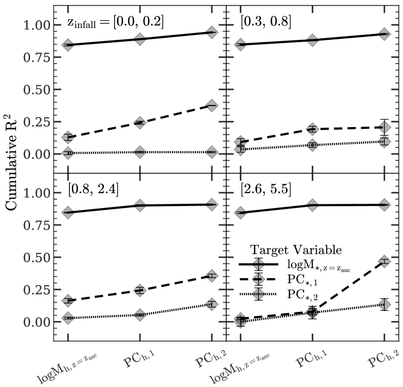
Figure 2: Cumulative $R^{2}$ of the regressor $\mathbb{R}$ in the model of central galaxies trained by TNG. Each panel shows the result for one piece of the model whose infall redshift range is indicated at the upper left corner of the panel. Error bars are estimated by the resampling method described in §4.1.

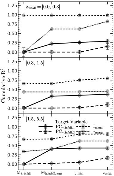
Figure 3: Cumulative $R^{2}$ of the mapping $\mathbb{R}_{\rm infall}$ in the model of satellite galaxies trained by TNG. Each panel shows the result for one piece of the model whose infall redshift range is indicated at the upper left corner of the panel. Error bars are estimated by the resampling method described in §4.1.

Figure 4: A comparison of galaxy $M_{\rm*,int}$ in the model $\rm TNG_{TNG}$ with the TNG simulation. Different panels show the results at different redshifts. In each panel, Red (blue) contours enclose the 1, 2, 3-$\sigma$ regions of central (satellite) galaxies, and gray shades are normalized histograms for central galaxies encoded by the color bar.

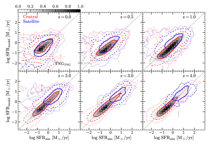
Figure 5: A comparison of galaxy SFR in the model $\rm TNG_{TNG}$ with the TNG simulation. Different panels show the results at different redshifts. In each panel, Red (blue) contours enclose the 1, 2, 3-$\sigma$ regions of central (satellite) galaxies, and gray shades are normalized histograms for central galaxies encoded by the color bar.

4 Results

As discussed in §1 and §2, MAHGIC can be trained by a hydrodynamic simulation, and applied to DMO simulations to make copies. Here we use subhalos and merger trees from TNG or EAGLE as the training data sets. As a consistency check, the trained model is first applied to the hydrodynamic simulation itself, but with all the information about the baryonic components discarded. Because of the impact of baryonic process, dark matter halo properties in a hydrodynamic simulation are not expected to be identical to those in the corresponding DMO simulation. The check serves as a test of the importance of this impact. The model is then applied to the two DMO simulations, TNG-Dark and ELUCID. In this section, we show results only for the model trained by TNG, while the results of the EAGLE-trained model are presented in Appendix B. For convenience, we refer the applications of the TNG-trained model to TNG, TNG-Dark, and ELUCID as $\rm TNG_{TNG}$, $\rm TNG\scalebox{0.5}[1.0]{$-$}Dark_{TNG}$, and $\rm ELUCID_{TNG}$, respectively, while using a subscript ‘EAGLE’ to denote the applications of the EAGLE-trained model.

To achieve a sufficiently high accuracy, we use $N_{\rm piece}=4$ and $(z_{1},z_{2},z_{3},z_{4})=(0.25,0.75,2.5,5.5)$ to model central galaxies, and $N_{\rm piece}=3$ and $(z_{1},z_{2},z_{3})=(0.3,1.5,5.5)$ for satellites. We note that these choices are made for the training data used here, and that different choices can be made when required by the constraining data. Tree branches with $z_{\rm infall}>5.5$ are not included in the model, but the galaxies in the modeled branches can extend to $z>5.5$.

4.1 The importance of individual predictor variables

As discussed in §3.1, MAHGIC is made interpretable by using the PCA to reduce the dimensionality of variables, and the GBDT to build the mapping between halos and galaxies. Such interpretability enables us to quantify the importance of halo properties to a given galaxy property, as well as to estimate the uncertainty in the predicted galaxy property. To measure model uncertainties and the importance of predictor variables, we show in Figure 2 the cumulative $R^{2}$ of the mapping $\mathbb{R}$ for the model of central galaxies trained by TNG. Briefly, $R^{2}$ is a value between 0 and 1, with $R^{2}=1$ indicating no uncertainty in the prediction of the target variable and $R^{2}=0$ indicating no correlation between the predictor variable and the target variable (see, Chen et al., 2021, for a detailed description). The $R^{2}$-value for each target variable is computed by building a series of GBDT regressors that use an increasing number of predictor variables in $\tilde{\mathrm{{\bf x}}}_{\rm h}$. For each regressor, a fraction of $75\%$ of all the branches in the sample are drawn randomly without replacement and used as the training set, and the remaining $25\%$ are used as the test set to compute $R^{2}$. The training and test processes are repeated 20 times, and the standard deviation of the $R^{2}$-value among them is used as an estimate of the error bars. The results shown in Figure 2 indicate that the $M_{\rm*,int}$ at the anchor redshift is dominated by the halo mass at this redshift, and that more than $80\%$ of the $R^{2}$ can be achieved by using only one halo property. Adding PCs only leads to limited improvements. This is consistent with the result in Paper-I where it was found that the stellar mass and SFR at a given redshift are almost totally determined by $v_{\rm max}$, and that adding PCs only leads to small variances around the predicted mean SFH. The $R^{2}$ value for the target $\rm PC_{*,1}$ is lower, typically less than $50\%$, even if all the three predictor variables of halos are used. For all redshifts, the contribution to $\rm PC_{*,1}$ made by the PCs of the subhalo MAH is significant in comparison to that of the halo mass, indicating that the shape of the SFH of a galaxy is affected by the shape of the MAH of its host halo. The $R^{2}$-value for $\rm PC_{*,2}$ is small, indicating that the detailed variations in the SFH are generated by complicated physical processes not well captured by using a small set of halo predictors. The poor performance of the model on $\rm PC_{*,2}$ also indicates that it is not useful to include more higher order PCs in the model.

Figure 3 shows the cumulative $R^{2}$ curves of the mapping $\mathbb{R}_{\rm infall}$ for the satellite model trained by TNG. The $R^{2}$ curves and error bars are computed in the same way as for the central model. Using $M_{\rm h,infall}$, $M_{\rm h,infall,cent}$ and $j_{\rm infall}$ is sufficient to correctly predict both $I_{\rm merge}$ and $\tau_{\rm merge}$, where $M_{\rm h,infall,cent}$ is not significant for $I_{\rm merge}$ and $j_{\rm infall}$ only helps for $\tau_{\rm merge}$ at high z. Including $z_{\rm infall}$ makes a significant improvement only for $\tau_{\rm merge}$ for subhalos in the piece of lowest $z_{\rm infall}$. However, since only a small fraction ($\sim 3\%$) of the galaxies hosted by such subhalos will merge with their centrals by $z=0$, the accuracy of the prediction for $\tau_{\rm merge}$ in this piece does not matter much. The $R^{2}$ values that can be reached for $\rm PC_{*,infall,1}$ and $\rm PC_{*,infall,2}$ are less than $50\%$ even when all the four halo properties are used, indicating that the SFH of a galaxy after infall is affected by many nuanced factors and cannot be modeled fully by using only a small set of halo properties at the infall time. The small $R^{2}$ for $\rm PC_{*,infall,2}$ suggests that including more PCs of the SFH in the model is not helpful. The contribution to $\rm PC_{*,infall,1}$ from $z_{\rm infall}$ is not significant, indicating that the dominant mode of the SFH after infall does not change significantly over each of the redshift intervals in question.

4.2 Stellar Mass and Star Formation Rate

Because the model is trained using TNG, a comparison of the predicted galaxy population with that given by TNG provides a direct check on the the performance of our method. Figure 4 shows a comparison of $M_{\rm*,int}$ predicted by $\rm TNG_{TNG}$ with that given by the TNG simulation for individual galaxies. Results for central and satellite galaxies are shown separately at different redshifts. As one can see, the model prediction matches well with the TNG simulation, without any significant bias. This demonstrates that our multi-stage, non-linear model is flexible enough to capture the main properties in the underlying halo-galaxy mapping in the simulation. The relation between the modeled $M_{\rm*,int}$ and the simulated $M_{\rm*,int}$ is also tight, with a standard deviation typically of 0.14 dex (0.17 dex) for central (satellite) galaxies at $z=0$ and 0.23 dex (0.26 dex) at $z=4$. This can be attributed to the use of a piece-wise approach, in which the mapping is trained over the whole redshift range.

Figure 5 shows the comparison of $\rm TNG_{TNG}$ with the TNG simulation for the SFR of individual galaxies at different redshifts. Again, we do not see any significant bias in the predictions of $\rm TNG_{TNG}$. Compared to $M_{\rm*,int}$, the relation of the SFR between $\rm TNG_{TNG}$ and the TNG simulation has larger scatter, with a standard deviation of 1.2 dex (1.5 dex) for central (satellite) galaxies at $z=0$ and 0.31 dex (0.46 dex) at $z=4$. This is expected, because SFR is a differential property, while $M_{\rm*,int}$ is cumulative. As demonstrated in Paper-I, SFR may be more sensitive to nuanced factors that are difficult to capture using a well-defined set of halo properties.

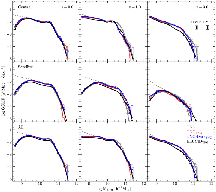
Figure 6: GSMFs of modeled galaxies compared with simulated ones. The model is trained using the TNG simulation. The first, second and third rows show the GSMFs of central, satellite and all (central+satellite) galaxies, respectively. Different columns show the GSMFs at different redshifts. Solid gray lines are from TNG simulation. Red, blue and gray lines are the results when the model is applied to TNG, TNG-Dark and ELUCID simulations, respectively. Dashed gray lines are GSMFs of all TNG simulated galaxies including those in the subhalos not selected in our samples. Error bars are computed by using 50 bootstrap resamplings. The left of the two vertical bars in the upper right panel indicates the difference in GSMF between TNG-$\rm Dark_{TNG}$ and $\rm ELUCID_{TNG}$ at $M_{\rm*,int}\in[1.0,5.0]\times 10^{10}\,h^{-1}{\rm M_{\odot}}$. The right one indicates the difference caused by the difference in HMF between the two simulations.

4.3 Galaxy Stellar Mass Function

When the model is applied to a DMO simulation, the results cannot be checked on the basis of individual galaxies, but can be tested statistically. One of the most important statistical properties of the galaxy population is the galaxy stellar mass function (GSMF), defined as the number density of galaxies as a function of stellar mass. Figure 6 compares the GSMFs obtained from TNG, $\rm TNG_{TNG}$, $\rm TNG\scalebox{0.5}[1.0]{$-$}Dark_{TNG}$ and $\rm ELUCID_{TNG}$, separately for central, satellite and all galaxies at five different redshifts. Because our sample selection criteria are based on dark matter halos above a certain mass, as described in §2.3, some galaxies are missed in our model. The difference between the gray solid curve and the gray dashed line in each panel of Figure 6 is caused by the sample selection. However, comparisons can still be made among TNG, $\rm TNG_{TNG}$, $\rm TNG\scalebox{0.5}[1.0]{$-$}Dark_{TNG}$ and $\rm ELUCID_{TNG}$ over the entire mass range because the same sample selection criteria are used for all of them.

The difference of GSMFs between TNG and $\rm TNG_{TNG}$ is small for both central and satellite galaxies at all redshifts. Key features of the GSMF, such as the power-law shape at the low-mass end and the rapid drop at the high-mass end, are well reproduced in $\rm TNG_{TNG}$. This is consistent with the result discussed in §4.2 that our model has no significant bias in $M_{\rm*,int}$ and SFR.

The GSMFs obtained from $\rm TNG\scalebox{0.5}[1.0]{$-$}Dark_{TNG}$ are very similar to those from $\rm TNG_{TNG}$, for both central and satellite galaxies and at all redshifts. This is a direct consequence of our model strategy (§3.1): we intentionally avoid the use of predictors that can be significantly affected by baryonic processes. In addition, our use of PCA and GBDT suppress the complexity of the model so as to avoid over-fitting the training data.

In the application of the model to ELUCID, more factors can affect the output. From Figure 6 one can see some noticeable differences between $\rm ELUCID_{TNG}$ and $\rm TNG\scalebox{0.5}[1.0]{$-$}Dark_{TNG}$. For central galaxies at $z\geqslant 1$, the GSMF of $\rm ELUCID_{TNG}$ is lower than that of $\rm TNG\scalebox{0.5}[1.0]{$-$}Dark_{TNG}$ in the intermediate mass range. This is produced, at least partly, by the lower halo mass function (HMF) of ELUCID at $z\geqslant 1$ compared to TNG-Dark, as shown in Appendix A. It may also be produced by a difference in the MAH of halos between the two simulations, although this difference is quite small, as shown in Appendix A. To see the effect of the lower HMF, we compute the difference of the GSMF between $\rm ELUCID_{TNG}$ and $\rm TNG\scalebox{0.5}[1.0]{$-$}Dark_{TNG}$, and compare it with the difference in HMF. The comparison is shown in the top right panel of Figure 6 using two bars for central galaxies with $M_{\rm*,int}\in[1.0,5.0]\times 10^{10}\,h^{-1}{\rm M_{\odot}}$ at $z=3$, where the difference in GSMF is the most significant. The difference in the GSMF is 0.28 dex, while the difference in the HMF is 0.30 dex in the corresponding halo mass range estimated from the $M_{\rm*,int}$-$M_{\rm h}$ relation. From this we conclude that the difference in the HMF, produced by the cosmic variance, is the most significant contributor to the difference in the GSMF. For satellites, the difference between $\rm ELUCID_{TNG}$ and $\rm TNG\scalebox{0.5}[1.0]{$-$}Dark_{TNG}$ is small at high-$z$, but becomes larger at $z\leqslant 1$, where the GSMF of ELUCID is lower than that of $\rm TNG\scalebox{0.5}[1.0]{$-$}Dark_{TNG}$ in the intermediate mass range. This is expected, given that $\rm ELUCID_{TNG}$ underestimates the number of central galaxies at $z>1$, which are potentially the progenitors of the satellite galaxies at lower $z$.

The GSMFs of the total population (centrals and satellites together) are shown in the third row of Figure 6. We see again that $\rm TNG_{TNG}$ and $\rm TNG\scalebox{0.5}[1.0]{$-$}Dark_{TNG}$ are both in good agreement with the TNG simulation. $\rm ELUCID_{TNG}$ underestimates the GSMF at $z>1$ in the intermediate stellar mass range. In general, the GSMF is dominated by centrals, more so at higher $z$.

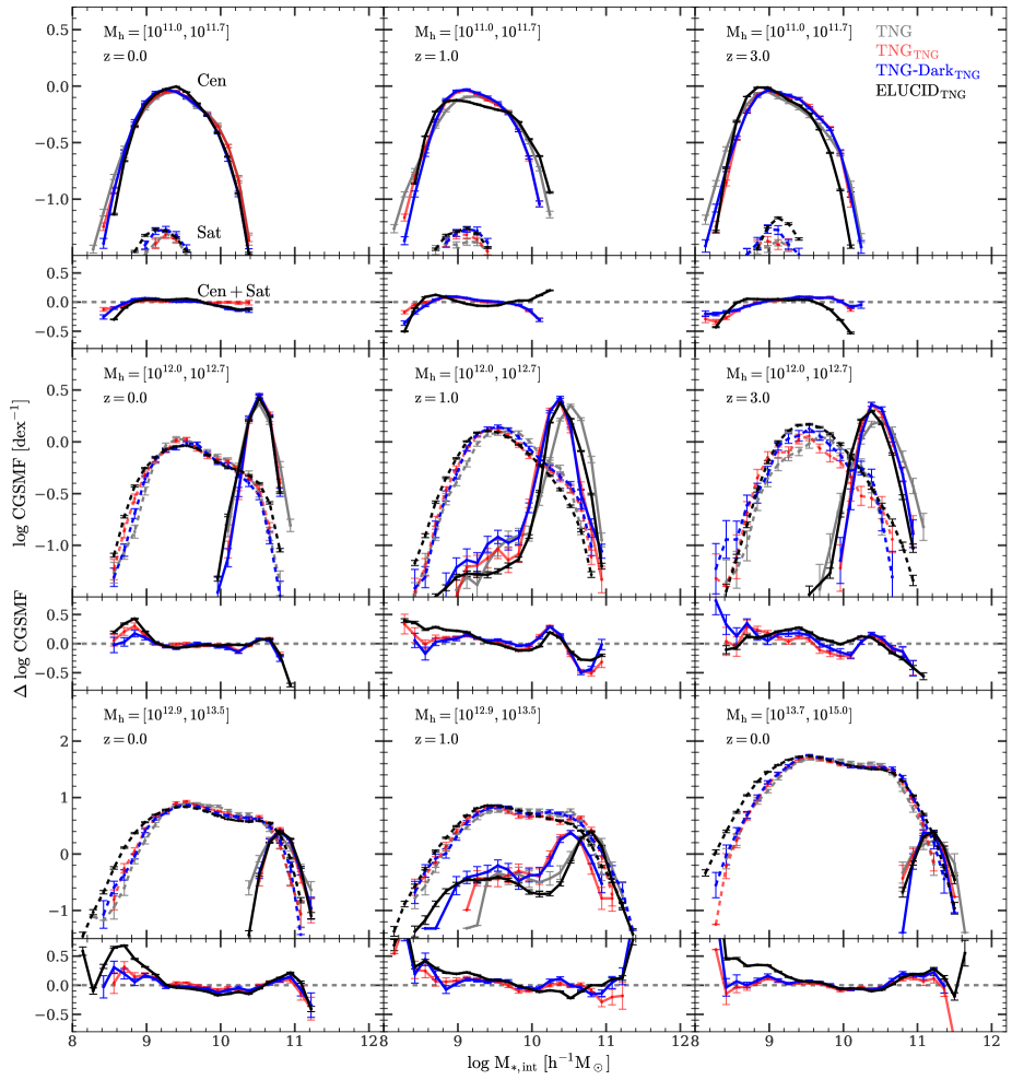
Figure 7: CGSMFs of dark matter halos with different halo masses $M_{\rm h}/(\,h^{-1}{\rm M_{\odot}})$ and at different redshifts as indicated in each panel. In each panel, gray lines are from the TNG simulation. Red, blue and black lines are results when the model is applied to TNG, TNG-Dark and ELUCID, respectively. Solid and dashed lines are for central and satellite galaxies, respectively. Error bars are computed by using 50 bootstrap resamplings. Each small panel shows the model residuals of CGMSFs relative to the TNG simulation for all (central+satellite) galaxies.

4.4 Conditional Galaxy Stellar Mass Functions

To check our model in more detail, we examine the conditional galaxy stellar mass function (CGSMF) for halos of different mass. This is a cleaner test, as it is not affected by variations in the halo mass function between the training simulation (TNG) and the target simulation (ELUCID) due to cosmic variance. Figure 7 shows the CGSMFs of centrals and satellites in FoF halos of different masses at different redshifts. Note that we do not show results for high-mass halos at high $z$ because such halos are too rare to give a reliable CGSMF. The results obtained from $\rm TNG_{TNG}$, $\rm TNG\scalebox{0.5}[1.0]{$-$}Dark_{TNG}$ and $\rm ELUCID_{TNG}$ are shown together and compared to the corresponding results obtained directly from the TNG simulation. As one can see, the CGMSFs of low-mass halos are dominated by centrals at all redshifts. As the halo mass increases, the peak of the central CGSMF moves rightward, as a result of the halo mass - central stellar mass relation. For high-mass halos, satellites dominate the CGSMF. For high-mass halos at high-$z$, for example, those with $M_{\rm h}/(\,h^{-1}{\rm M_{\odot}})\in[10^{12.9},10^{13.5}]$ at $z=1$, the CGMSFs of centrals in the TNG simulation have a tail at the low-mass end. Our model captures this feature, although it is unclear if the feature is physical.

In terms of the CGSMF, we see that $\rm TNG_{TNG}$ and $\rm TNG\scalebox{0.5}[1.0]{$-$}Dark_{TNG}$ match closely with each other at all redshift and for halos of different mass, and that both are compatible with the TNG simulation. This demonstrates again that our model is not significantly affected by uncertainties introduced by baryonic processes. The CGSMFs obtained from $\rm ELUCID_{TNG}$ also closely follow the TNG-based results, although some differences are noticeable. In general, the differences are not much larger than the variances among the TNG-based results, indicating that our model is valid for any DMO simulation where the dark matter halo population is modeled reliably.

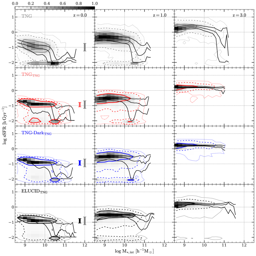
Figure 8: The galaxy distribution in the $\log M_{\rm*,int}$-$\log$ sSFR plane. Different columns show the results at different redshifts indicated in the first row. The first row shows the result from the TNG simulation. The other three rows show the results when the model is applied to TNG, TNG-Dark and ELUCID, respectively. In each panel, gray shades are normalized histograms encoded by the color bar. Solid, dashed and dotted contours enclose 1,2,3-$\sigma$ regions, respectively. The black solid lines show the $25\%$, $50\%$ and $75\%$ quantiles of $\log{\rm sSFR}$ at a given $M_{\rm*,int}$. The gray bar in the top left panel indicates the 1-$\sigma$ scatter of the main sequence at $M_{\rm*,int}\sim 10^{10}\,h^{-1}{\rm M_{\odot}}$ computed directly from the simulated data. The colored bars in other left panels show the scatter of the modeled galaxies while the gray bars show the scatter after the missed random component is added.

4.5 The Star-forming Main Sequence and Galaxy Bimodality

The galaxy distribution in the $\rm\log sSFR$ - $\log M_{\rm*,int}$ space is observed to be bimodal. The mode with high sSFR is referred to as the star-forming main sequence, while the one with lower sSFR is referred to as the quenched population. This bimodal distribution was first established observationally (e.g. Strateva et al., 2001; Blanton et al., 2003; Baldry et al., 2004; Li et al., 2006; Faber et al., 2007; Brammer et al., 2009; Coil et al., 2017), and later reproduced in some hydrodynamic simulations, such as the TNG simulation (Nelson et al., 2018). The bimodal distribution contains important information about galaxy formation and evolution, and should be reproduced in any successful model.

Figure 8 shows, in the first row, the distribution of galaxies at different redshifts in the $\rm\log sSFR\scalebox{0.5}[1.0]{$-$}\log M_{\rm*,int}$ plane obtained directly from the TNG simulation. The predictions of $\rm TNG_{TNG}$, $\rm TNG\scalebox{0.5}[1.0]{$-$}Dark_{TNG}$ and $\rm ELUCID_{TNG}$ are shown in the subsequent rows, respectively. Because of the limited resolution, TNG cannot resolve the star formation activity reliably when the SFR is too low. These low-SFR galaxies are stacked at the bottom of each panel in the first row of Figure 8, which has the effect of artificially making the 1-$\sigma$ contours of the quenched population tight. As one can see, TNG galaxies show a strong bimodal distribution at low $z$, but the quenched population decreases with increasing $z$ and disappears at $z=3$. The majority of the galaxy population in the TNG simulation start from a well-defined star-forming sequence at high $z$, and become quenched subsequently. The quenching starts from the massive end at $z\sim 3$ and moves to lower mass at lower $z$.

The results obtained from the three applications, $\rm TNG_{TNG}$, $\rm TNG\scalebox{0.5}[1.0]{$-$}Dark_{TNG}$ and $\rm ELUCID_{TNG}$, are all comparable with each other. At a given $z$, all the models predict star-forming main-sequences with a similar amplitude and dispersion. The predicted sequences have amplitudes similar to those given by the TNG simulation, but with smaller dispersion, particularly at $z=0$. This indicates that our model, which is based on a limited number of predictors (halo properties), is not able to capture all the variances in the SFR. As demonstrated in Paper-I, more than $50\%$ of the main sequence scatter at $z=0$, as measured by the $R^{2}$ of the GBDT regressors, is contributed by nuanced factors that are difficult to relate to halo properties. One possible way to correct for this, as proposed in Paper-I, is to include a random component, whose variance is characterized by the difference between the required variance and the modeled variance of $\log{\rm sSFR}$ in the main sequence. Here we can obtain this by comparing the main sequence galaxies in the simulation and in our model. The vertical bars in Figure 8 show the effects of adding a random component to the modeled galaxies at $z=0$. The main-sequence scatter is enlarged significantly for the three application cases, and the predicted scatter is now comparable to that given by the TNG simulation. Overall, the predicted 2-$\sigma$ contours in the three application cases are comparable to those obtained from the TNG simulation. At low $z$, our model predicts an extended quenched population, consistent with the simulation, but the predicted quenched population at the high-stellar-mass end is smaller than in the TNG simulation, as seen from the $50\%$ and $75\%$ percentile lines. This discrepancy arises from the difficulty in predicting whether or not a high-mass galaxy is quenched solely on the basis of halo properties, as shown in Paper-I. The predicted quenched population in the low stellar mass range at $z=0$ is also more diffuse in the three application cases. As shown in Paper-I, this is a result of sample imbalance: low-mass galaxies in TNG at $z\sim 0$ are mainly star-forming galaxies, and our model is more concentrated on the star-forming population, leaving the quenched population less well modeled.

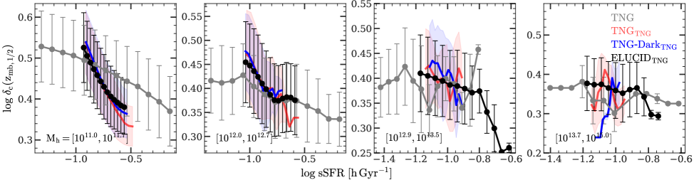
Figure 9: The relation between subhalo formation time $z_{\rm mb,1/2}$ and sSFR for $z=0$ central subhalos. Only the star-forming population (${\rm sSFR}\geqslant 10^{-2}\,h^{-1}{\rm Gyr}$) is shown. Each panel shows the result for subhalos with a given halo mass as indicated at the lower left corner of the panel. Gray lines show the result from TNG simulation. Red, blue and black lines are results when we apply the TNG-trained model to TNG, TNG-Dark and ELUCID, respectively. Error bars and shades are standard deviations in bins.

4.6 The Correlation of Star Formation with Halo Assembly

Because of the inclusion of MAH PCs in our model, galaxy properties predicted by the model are naturally correlated with the MAH of the host halos. In Figure 9, we show the relation between the halo half-mass formation time, $z_{\rm mb,1/2}$, and the current sSFR for central star-forming galaxies at $z=0$. Here $z_{\rm mb,1/2}$ is calculated by tracing the main branch in a subhalo merger tree rooted in the target subhalo, and the redshift is represented by

$$\delta_{\rm c}(z)=\frac{\delta_{\rm c,0}}{D(z)},$$ (12)

where $\delta_{\rm c,0}=1.686$ is the critical overdensity given by the spherical collapse model, and $D(z)$ is the linear growth factor at $z$ given by Carroll et al. (1992).

As described at the end of §3 and shown in §4.5, the modeled sSFR is missing a random component that cannot be fully explained by the halo properties considered here. Consequently, the predicted sSFR for star-forming galaxies spans a smaller range than that given by the simulation. The relatively small dynamic range in $\log{\rm sSFR}$ shown in Figure 9 for the three application cases is caused by this. Taking into account the random component, our model actually reproduces the trends seen in the simulation: galaxies in halos of larger $\delta_{\rm c}(z_{\rm mb,1/2})$ tend to have smaller sSFR. The only exception is for massive systems, where the uncertainty is too large to see the correct trend in $\rm TNG_{TNG}$ and $\rm TNG\scalebox{0.5}[1.0]{$-$}Dark_{TNG}$. We also note that the correlation between halo assembly and sSFR is weak, and the variance between individual galaxies is large, as can be seen from the large error bars and shadings shown in Figure 9.

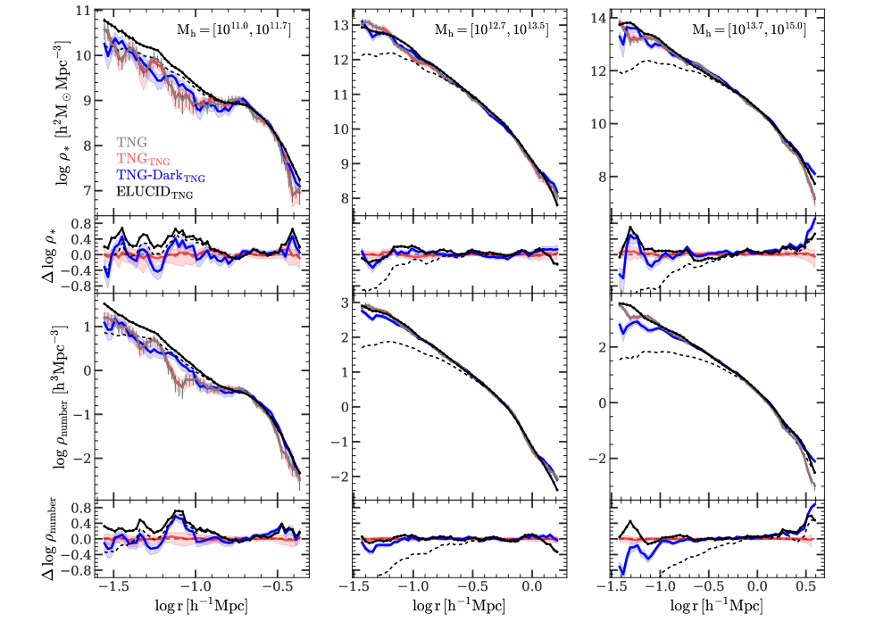
Figure 10: The $z=0$ $M_{\rm*,int}$ density profile (first row) and number density profile (second row) of satellite galaxies in dark matter halos with different $M_{\rm h}/(\,h^{-1}{\rm M_{\odot}})$ indicated in the panels of first row. In each panel, gray line is from TNG simulation. Red, blue and solid black lines are results when the model is applied to TNG, TNG-Dark and ELUCID respectively. The dashed black line is also for ELUCID, but only shows the subhalos that are resolved by the simulation. Error bars and shades represent the standard deviation computed using 50 bootstrap resamplings. Each small panel shows the residuals of curves relative to the gray line in the same panel.

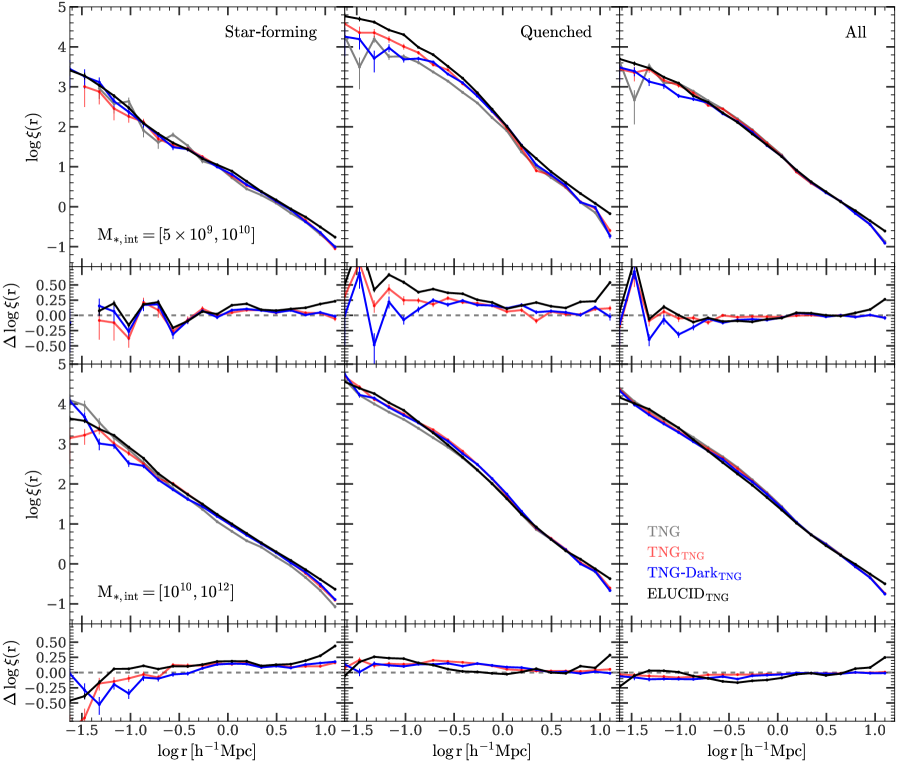
Figure 11: The auto-correlation functions for galaxies at $z=0$ with different $M_{\rm*,int}/(\,h^{-1}{\rm M_{\odot}})$ (rows). Results for star-forming, quenched, and all (star-forming + quenched) galaxies (divided at ${\rm sSFR}=5\times 10^{-1}\,h\,{\rm Gyr}^{-1}$) are shown separately in the three columns. Error bars represent the standard deviation computed using 50 bootstrap resamplings. In each panel, gray line is from TNG simulation. Red, blue and black lines are results of the model applied to TNG, TNG-Dark and ELUCID, respectively. Each small panel shows the residuals of the corresponding curves relative to the gray line in the same panel.

4.7 The Spatial distribution of satellite galaxies in dark matter halos and the two-point correlation function

Galaxy clustering is a commonly used statistical property to characterize the spatial distribution of the galaxy population. From a theoretical perspective, the galaxy-galaxy correlation can be decomposed into two components: the ‘two-halo term’, which describes the correlation produced by the halo-halo correlation, and the ‘one-halo term’, which is produced by the galaxy distribution in individual dark matter halos. The two-halo term on large scales is determined as long as the halo occupation of galaxies is correctly modeled. The ‘one-halo term’, on the other hand, depends on the details of the galaxy distribution in halos. Since our model reproduces the CGSMF in halos of different mass (§4.4), it is already tested for its predictions for halo occupation. Here we first present test results for the predicted galaxy distribution inside halos.

In MAHGIC, galaxies are modeled based on their host subhalos and their positions are assumed to be the same as the positions of the most bound particles of the corresponding subhalos. Thus, as long as the DMO simulations correctly predict the distribution of subhalos in their host halos, the galaxy distribution will also be reproduced as long as the subhalo-galaxy interconnection is correctly predicted. Figure 10 shows the stellar mass density profile and number density profile of satellite galaxies in halos of different masses at $z=0$. The three application cases, $\rm TNG_{TNG}$, $\rm TNG\scalebox{0.5}[1.0]{$-$}Dark_{TNG}$ and $\rm ELUCID_{TNG}$ are all plotted and compared to the TNG simulation. As described in §3.3, we have to follow some satellite galaxies in ELUCID using merger times calibrated with high resolution-simulations, because their subhalos are not well resolved in ELUCID. These galaxies do not have simulated subhalos associated with them in ELUCID and, therefore, do not have subhalo-based positions. The results obtained without these galaxies are shown in Figure 10 as the dashed black curves. We can look at the results in three steps. First, the results between TNG and $\rm TNG_{TNG}$ are almost indistinguishable for halos of different mass, indicating that the subhalo-galaxy interconnection predicted by our model is unbiased. This is consistent with the results, presented in §4.2, that the predicted $M_{\rm*,int}$ and SFR follow the simulation results closely. Second, comparing the results of $\rm TNG_{TNG}$ and $\rm TNG\scalebox{0.5}[1.0]{$-$}Dark_{TNG}$, we see that baryonic processes have some effects on the results. The red and blue lines in Figure 10 follow each other tightly over a large range of $r$. Some differences can be seen in the inner regions of halos ($r<0.1\,h^{-1}{\rm{Mpc}}$), where the number density of satellites predicted by $\rm TNG\scalebox{0.5}[1.0]{$-$}Dark_{TNG}$ is lower than that of $\rm TNG_{TNG}$, particularly for halos with $M_{\rm h}\geqslant 10^{12.7}\,h^{-1}{\rm M_{\odot}}$. Apparently, the baryonic component in a satellite can make its subhalo more concentrated and harder to destroy by environmental effects near the center of its host halo. The difference in the stellar mass density profile is smaller than that in the number density profile, indicating that the destroyed subhalos are preferentially of low mass. These are consistent with the results obtained by Simha et al. (2012) using subhalo abundance matching technique, where they found that the stellar mass loss can significantly affect the radial profile of low-mass galaxies in massive halos. Third, comparing the results between $\rm TNG\scalebox{0.5}[1.0]{$-$}Dark_{TNG}$ and $\rm ELUCID_{TNG}$, we can clearly see the effects of the simulation resolution. The difference between the blue and dashed black curves in Figure 10 is significant for halos above $M_{\rm h}=10^{12}\,h^{-1}{\rm M_{\odot}}$. This is expected, because the ELUCID simulation has a much lower resolution and subhalos can go below the mass resolution limit or be disrupted artificially before they merge with the central subhalo (e.g., Green et al., 2021). The underestimates of the galaxy stellar mass and number densities are more significant in higher mass halos because, at a given $r$, the mass density is higher in halos of higher mass. At large $r$ where subhalos are resolved in ELUCID, the predicted profiles tightly follow those of the TNG simulation. Note that we only use halo properties at the infall time to model satellite galaxies, which has the advantage of being independent of resolution issues and artificial disruption after infall.

To account for the numerical effects on the density profile of satellite galaxies, we match each FoF halo in ELUCID to a FoF halo in TNG-Dark that has the same redshift and $M_{\rm h}$. The satellite galaxies in ELUCID that do not have associated subhalos are assigned positions using the subhalos in the matched halo from TNG-Dark. The results obtained by including these subhalos are shown in Figure 10 as the solid black curves. The match between the TNG-Dark and the ELUCID results are now much better for all halos with $M_{\rm h}\geqslant 10^{12.0}\,h^{-1}{\rm M_{\odot}}$. For small halos with $M_{\rm h}\in[10^{11},10^{11.7}]\,h^{-1}{\rm M_{\odot}}$, the comparison cannot be easily made, because the TNG and TNG-Dark results have large fluctuations owing to the limited sample size. This again demonstrates the effects of cosmic variance and the importance of combining the two types of simulations to construct statistically reliable mock samples.

For completeness, Figure 11 shows the auto-correlation function for the total galaxy population, and separately for star-forming and quenched populations in two stellar mass bins. In all cases, there is a moderate difference between the TNG simulation and our model results. The largest difference is seen for the quenched low-mass population dominated by small satellite galaxies. This is the case because of the inaccuracy of our model in predicting the quenched fraction in the low-mass population, as discussed in §4.5.

To conclude, our model correctly reproduces the satellite distribution in dark matter halos, as long as their subhalos can be resolved in the DMO simulation. For subhalos whose positions cannot be followed reliably in a large-volume DMO simulation, their positions can be modeled statistically using calibrations based on high-resolution DMO simulations. Thus, MAHGIC also provides a reliable prescription to model the spatial distribution of galaxies.

5 Summary and Discussion

In this paper, we develop a model, MAHGIC (Model Adapter for the Halo-Galaxy Inter-Connection), to establish the interconnection between galaxies and dark matter halos. The model uses a set of halo (subhalo) properties, such as halo mass, MAH and orbit, as model input, and transforms it into a set of galaxy properties, such as stellar mass and SFH. We use PCA and GBDT to help the model design, and incorporate them into the model pipeline. We use two sets of hydrodynamic simulations, TNG and EAGLE, to train the model, and apply it to a large DMO simulation, ELUCID, to demonstrate the reliability, flexibility and accuracy of our model. The key points and the main results that we obtain in the feature selection, model design, training and testing are summarized below.

We select a set of subhalo properties and a set of galaxy properties as the predictors and target variables of the model, respectively. This feature selection, based on the methods and results described in Chen et al. (2020) and Paper-I, can be summarized as follows:

1. Only the most important subhalo properties are selected as the predictors of galaxy stellar properties. Properties (e.g., halo structural and environmental properties) that are strongly degenerate with other more important properties (e.g., halo mass, MAH) are not used. We also avoid the use of subhalo properties that are sensitive to baryonic processes. Subhalo properties that are not well resolved in large DMO simulations, such as the halo MAH at high redshift and the surviving time of subhalos after being accreted by their hosts, are modeled using calibrations of high-resolution simulations. The final set of subhalo properties used by MAHGIC include halo mass, the MAH and the orbit. The set of stellar properties used as the target variables are stellar mass and SFH of individual galaxies. These quantities can be used to obtain the SFR and quenching status at any given redshift.

2. We apply PCA to the MAH of subhalos and the SFH of galaxies, and transform them into sets of PCs in spaces of lower dimensions. This data compression step gives a set of linearly-independent PCs, further reducing the degeneracy among subhalo properties. The use of PCs can reduce the model complexity by eliminating high-order PCs that are not constrained by the data. It also makes the model adaptable - more PCs can be included to accommodate additional constraints from new data, as guided by the Bayesian theory. As shown in Chen et al. (2020), PCs of halo MAH are interpretable because of their linear nature, as seen from their tight correlations with various quantities characterizing the formation of subhalos.

MAHGIC provides a full pipeline to map subhalo properties to galaxy properties, and the main steps in its construction are summarized below.

1. We use GDBTs to map subhalo properties to galaxy properties in spaces of reduced dimensions. The tree-based method is capable for building highly non-linear relationships between variables, which is important for our problem. GBDT uses an ensemble of randomized trees to overcome over-fitting, hence ensuring the robustness of our model. GBDT also provides summary statistics, such as feature importance $\mathcal{I}$ and $R^{2}$, to help understand the interaction among different variables, making the model interpretable.

2. We model central and satellite galaxies separately, and break the reconstruction of the SFH into several redshift pieces. This multi-component and multi-stage treatment of the SFH allows the model to be adapted to the availability of constraining data at different redshifts.

3. As a demonstration of the performance of MAHGIC, we use the hydrodynamic simulation, TNG, to train the model, and apply the trained model to dark matter halos given by TNG, TNG-Dark and ELUCID. The comparison between the TNG results and the outputs of these applications verifies that the model is both reliable and flexible. We also train our model using an independent hydrodynamic simulation, EAGLE, and the results provide further support to our conclusion.

4. The test using DMO simulations shows that our model can reproduce a variety of statistical properties of the galaxy populations in the training hydrodynamic simulations. The predicted $M_{\rm*,int}$ and SFR for individual galaxies are unbiased, with a well-controlled dispersion relative to the true values. The GSMFs at different redshifts, and the CGSMFs in halos of different $M_{\rm h}$, are well recovered. The star-forming main sequence and the galaxy bimodality are well captured by our model. Even the weak correlation between galaxy sSFR and halo assembly time is also reproduced. Finally, the model prediction for the spatial distribution of galaxies in their host halos also matches that given by hydrodynamic simulations, indicating that MAHGIC is capable of modeling galaxy clustering.

The reliability, accuracy and flexibility of MAHGIC in recovering galaxy statistical quantities indicate that it can be used to make mocking copies of hydrodynamic simulations into DMO simulations with larger volumes. The copied galaxy population shares the same halo-galaxy interconnection with the training hydrodynamic simulation, while the larger sample provided by the DMO simulation provides a fairer representation of the galaxy population expected from the physical processes assumed in the hydrodynamic simulation. Therefore, MAHGIC provides an adapter to link these two types of simulations and to combine their individual advantages.

The general framework provided by MAHGIC can be extended to another type of applications that use observational data as constraints. In this case, the PCA templates of SFH trained from hydrodynamic simulations can still be used to reduce the complexity of the model, as long as the templates reflect the real star formation modes in the universe. Other parts of the pipeline can be adjusted accordingly to the observational data. For example, if the SFH cannot be obtained reliably from the observation, the corresponding variables, $\tilde{\mathrm{{\bf x}}}_{*}$, in the representation layer of galaxies, will become latent variables. The regressor, $\mathbb{R}$, can also be adjusted to a differentiable form, such as that of polynomials or neural networks, which allows the optimization to be made by a gradient-based method, such as the back-propagation algorithm (e.g., Rumelhart et al., 1986). Some optimization methods that do not require gradient computation may also be useful, such as the particle swarm method used by Moster et al. (2020) in the optimization of a network-based model. Other optimization methods specific to models with latent variables, such as the expectation-maximization (EM) algorithm, the more general variational inference algorithm, and the sampling method for Bayesian networks (e.g., Bishop, 2006; Lu et al., 2011, 2012; Behroozi et al., 2019) , may also be used to optimize the model. We will come back to this when we apply the model to observational data.

Data availability

The data and software used in this article will be available from the corresponding author. They are also available at https://lig.astro.tsinghua.edu.cn/.

The computation was supported by the HPC toolkit HIPP at https://github.com/ChenYangyao/hipp.

Appendix A Robustness of Subhalo Properties in the Simulations

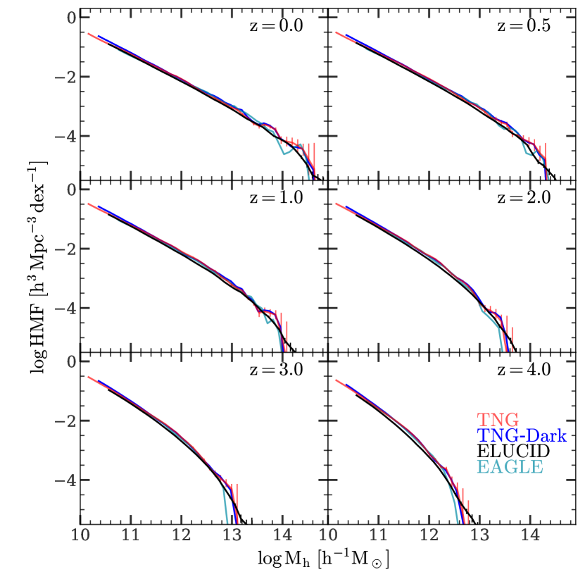
Figure 12: HMFs in TNG (red), TNG-Dark (blue), ELUCID (black) and EAGLE (green) simulations. Each panel shows the HMFs at a given redshift indicated in the upper-right corner of the panel. Error bars are computed by using 50 bootstrap resamplings.

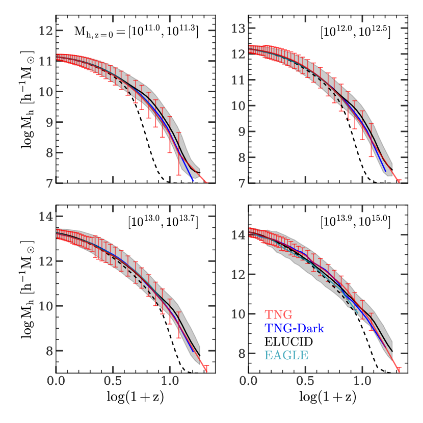
Figure 13: MAHs of $z=0$ central subhalos with different masses $M_{\rm h}/\,h^{-1}{\rm M_{\odot}}$ as indicated in each panel. In each panel, the red, blue and green lines are from the TNG, TNG-Dark and EAGLE simulations, respectively. The black solid line is from the ELUCID simulation, extended using TNG-Dark at high redshift. The black dashed line is from the ELUCID simulation without any extension. Error bars and shades are standard deviations among halos in TNG and ELUCID (with extension), respectively.

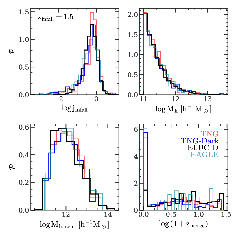
Figure 14: Distributions of satellite subhalo properties. The subhalo properties shown in the four panels are normalized orbital angular momentum, satellite subhalo mass, subhalo mass of the central subhalo that hosts the satellite, and the merger time. The first three are computed at the infall-time. Red, blue, black, and green histograms are from TNG, TNG-Dark, ELUCID and EAGLE simulations, respectively. All subhalos with $z_{\rm infall}=1.5$ are shown.

In this paper, we use dark matter halo/subhalos from TNG, TNG-Dark, ELUCID and EAGLE simulations as model input. These subhalos are mapped to galaxies using an interpretable deep model. In this appendix, we describe in detail the halo properties that are used in our analyses. One requirement of our model on the halo properties is that they must be stable, not sensitive to baryonic effects and numerical resolution (see §3.1).

Figure 12 shows the halo mass functions (HMFs) at different redshifts in the three simulations. The HMFs of TNG, TNG-Dark and EAGLE almost overlap with each other except at the high-mass end, where statistics are poor. This indicates that the halo mass is a stable physical quantity that is not affected much by baryonic processes and not significantly different in different hydrodynamic simulations. The ELUCID HMFs are slightly lower than those of TNG, TNG-Dark and EAGLE. This is because ELUCID assumes a slightly different cosmology and has a lower mass resolution.

One advantage of first training an empirical model with small-volume, high-resolution hydrodynamic simulations and then applying it to large-volume DMO simulations is that more robust statistics can be drawn from the modeled galaxies in the DMO simulations. This can be seen in Figure 12, where the HMFS at the high-mass ends in TNG and EAGLE are both noisy, but the HMF of ELUCID remains stable and has a only small scatter even for halos with $M_{\rm h}>10^{14}\,h^{-1}{\rm M_{\odot}}$ at low $z$.

Since in our model galaxy properties are related not only to the current state of dark matter halos, but also to their mass assembly histories (MAH) we, therefore, need to check the subhalo MAH given by different simulations. Figure 13 shows the MAH of $z=0$ subhalos with different masses. The MAH in TNG, TNG-Dark and EAGLE have no obvious differences, indicating the robustness of this halo property used in our model. Without any modification, the mass in the mean MAHs (black dashed lines) of ELUCID halos is significantly underestimated at high-$z$ when most halos are below the resolution limit of $6\times 10^{9}\,h^{-1}{\rm M_{\odot}}$.

As mentioned in §2.3, we use halo merger trees given by TNG-Dark to complete the missing parts of the MAH of ELUCID halos up to sufficiently high redshift. The extended MAHs, shown in Figure 13 as black solid lines, are comparable to the MAHs given by TNG, TNG-Dark and EAGLE. This extension largely eliminates the difference caused by numerical resolution, allowing the application of our model to the ELUCID simulation.

A number of properties for satellite subhalos are also used in our model, and here we check their reliability in different simulations. As an example, Figure 14 shows the distributions of these properties for all subhalos with $z_{\rm infall}=1.5$. Only small differences can be seen in the distributions of $\log j_{\rm infall}$, $M_{\rm h}$, and $\log M_{\rm h,cent}$ between ELUCID and the other three simulations. This can lead to some differences in the model predictions for satellite galaxies as seen in §4. In contrast, the merger time, $z_{\rm merge}$, obtained from ELUCID is quite different from those obtained from TNG, TNG-Dark and EAGLE. Many subhalos in the high-resolution simulations can survive to $z=0$, while a large fraction of subhalos in ELUCID are destroyed too early owing to the limited resolution. This affects our model by directly reducing the number of satellite subhalos. In §3.3, we solve this problem by using a model that predicts the merger time from other, more robust halo properties.

Appendix B Training with and Application to the EAGLE Simulation

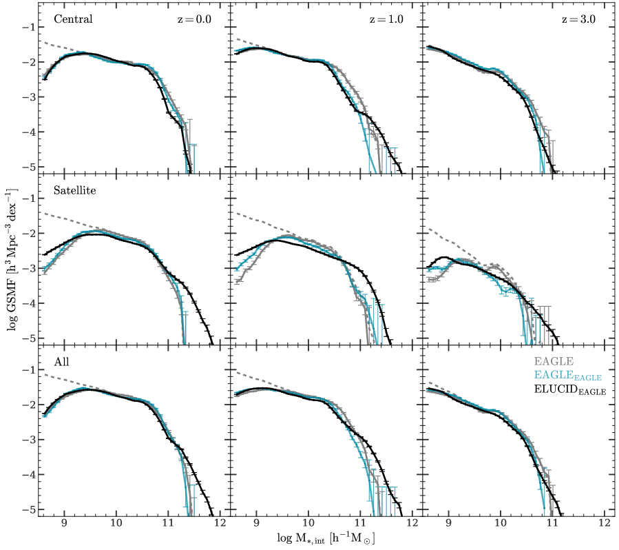
Figure 15: The GSMFs of modeled galaxies trained by EAGLE in comparison with EAGLE simulated ones. The first, second and third rows show the GSMFs of central, satellite and all (central+satellite) galaxies, respectively. Different columns show the GSMFs at different redshifts. Solid gray lines are from the EAGLE simulation. The green and black lines are the results when the model is applied to the EAGLE and the ELUCID simulations, respectively. The dashed gray lines are GSMFs of all EAGLE galaxies including those in the subhalos not selected in our samples. Error bars are computed by using 50 bootstrap resamplings.

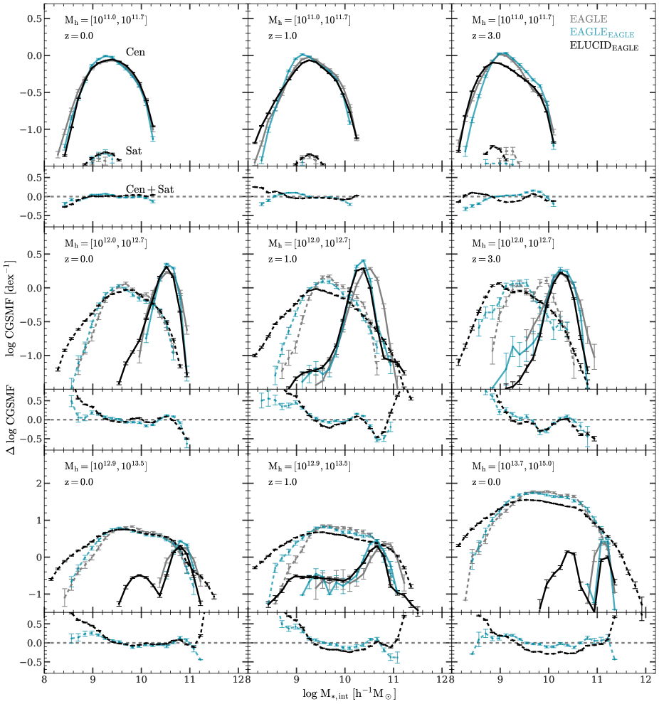
Figure 16: The CGSMFs of dark matter halos with different halo masses $M_{\rm h}/(\,h^{-1}{\rm M_{\odot}})$ and at different redshifts indicated in each panel. In each panel, the gray lines are from the the EAGLE simulation. The green and black lines are results when the model is applied to EAGLE and ELUCID, respectively. Solid and dashed lines are for central and satellite galaxies, respectively. Error bars are computed by using 50 bootstrap resamplings. Each small panel shows the model residuals of CGMSFs relative to the EAGLE simulation for all (central+satellite) galaxies.

In this appendix, we train MAHGIC using the EAGLE simulation, and then apply it to the subhalo merger trees obtained from both EAGLE and ELUCID. The model applied to EAGLE and ELUCID are referred to as $\rm EAGLE_{EAGLE}$ and $\rm ELUCID_{EAGLE}$, respectively.

To achieve this, several changes are made to the modeling process. The merger tree branches in ELUCID are extended using the matched branches in EAGLE, instead of those in TNG-Dark (§2.3). The training data are taken from EAGLE and the application is also made to EAGLE, instead of TNG (§4). All the other details, including the sample selection criteria, model pipeline and the separation redshifts, remain the same.

Figure 15 shows the GSMFs of EAGLE, $\rm EAGLE_{EAGLE}$ and $\rm ELUCID_{EAGLE}$ for central, satelite, and all galaxies at different redshifts from $0$ to $4$, respectively. As one can see, the GSMFs obtained from both $\rm EAGLE_{EAGLE}$ and $\rm ELUCID_{EAGLE}$ follow quite tightly those given by EAGLE. Overall, the performance of our model on EAGLE is very similar to its performance on TNG, indicating that the model is sufficiently flexible to accommodate different assumptions about galaxy formation represented by the two simulations. We note that EAGLE has a smaller volume than TNG, so the cosmic variance is expected to be larger. This can be seen from Figure 12, where the high mass end of EAGLE HMF is underestimated at $z\geqslant 2$. EAGLE also has a lower mass resolution and this can be seen from Figure 13 where the MAH of halos stops at lower redshift. EAGLE has 29 output snapshots, less than the 100 snapshots in TNG, so the training data are more limited. Taking these differences into consideration, the deviation of model results from EAGLE at the high stellar mass end of the GSMF can be explained. Figure 16 shows the CGSMFs obtained from EAGLE, $\rm EAGLE_{EAGLE}$ and $\rm ELUCID_{EAGLE}$ for central and satellite galaxies. Here we see again that our model performs well for halos of different mass, giving further support to its reliability and flexibility.

References

- Ade et al. (2014) Ade P. a. R., et al., 2014, A&A, 571, A16
- Ade et al. (2016) Ade P. a. R., et al., 2016, A&A, 594, A13
- Agarwal et al. (2018) Agarwal S., Davé R., Bassett B. A., 2018, MNRAS, 478, 3410
- Baldry et al. (2004) Baldry I. K., Glazebrook K., Brinkmann J., Ivezić Ž., Lupton R. H., Nichol R. C., Szalay A. S., 2004, ApJ, 600, 681
- Behroozi et al. (2019) Behroozi P., Wechsler R. H., Hearin A. P., Conroy C., 2019, MNRAS, 488, 3143
- Berlind & Weinberg (2002) Berlind A. A., Weinberg D. H., 2002, ApJ, 575, 587
- Bishop (2006) Bishop C. M., 2006, Pattern Recognition and Machine Learning. Springer
- Blanton et al. (2003) Blanton M. R., et al., 2003, ApJ, 594, 186
- Boylan-Kolchin et al. (2008) Boylan-Kolchin M., Ma C.-P., Quataert E., 2008, MNRAS, 383, 93
- Brammer et al. (2009) Brammer G. B., et al., 2009, ApJ, 706, L173
- Bryan & Norman (1998) Bryan G. L., Norman M. L., 1998, ApJ, 495, 80
- Carroll et al. (1992) Carroll S. M., Press W. H., Turner E. L., 1992, ARA&A, 30, 499
- Chabrier (2003) Chabrier G., 2003, PASP, 115, 763
- Chaves-Montero & Hearin (2020) Chaves-Montero J., Hearin A., 2020, MNRAS, 495, 2088
- Chaves-Montero & Hearin (2021) Chaves-Montero J., Hearin A., 2021, MNRAS, p. stab1831
- Chen et al. (2019) Chen Y., Mo H. J., Li C., Wang H., Yang X., Zhou S., Zhang Y., 2019, ApJ, 872, 180
- Chen et al. (2020) Chen Y., Mo H. J., Li C., Wang H., Yang X., Zhang Y., Wang K., 2020, ApJ, 899, 81
- Chen et al. (2021) Chen Y., Mo H. J., Li C., Wang K., 2021, MNRAS, 504, 4865
- Cohn (2018) Cohn J. D., 2018, MNRAS, 478, 2291
- Cohn & van de Voort (2015) Cohn J. D., van de Voort F., 2015, MNRAS, 446, 3253
- Coil et al. (2017) Coil A. L., Mendez A. J., Eisenstein D. J., Moustakas J., 2017, ApJ, 838, 87
- Cormen et al. (2009) Cormen T. H., Leiserson C. E., Rivest R. L., Stein C., 2009, Introduction to Algorithms, Third Edition, 3rd edn. The MIT Press
- Crain et al. (2015) Crain R. A., et al., 2015, MNRAS, 450, 1937
- Davis et al. (1985) Davis M., Efstathiou G., Frenk C. S., White S. D. M., 1985, ApJ, 292, 371
- Dolag et al. (2009) Dolag K., Borgani S., Murante G., Springel V., 2009, MNRAS, 399, 497
- Dunkley et al. (2009) Dunkley J., et al., 2009, ApJS, 180, 306
- Faber et al. (2007) Faber S. M., et al., 2007, ApJ, 665, 265
- Green et al. (2021) Green S. B., van den Bosch F. C., Jiang F., 2021, MNRAS, 503, 4075
- Guo et al. (2010) Guo Q., White S., Li C., Boylan-Kolchin M., 2010, MNRAS, 404, 1111
- Guo et al. (2016) Guo H., et al., 2016, MNRAS, 459, 3040
- He et al. (2016) He K., Zhang X., Ren S., Sun J., 2016, in Proceedings of the IEEE Conference on Computer Vision and Pattern Recognition. pp 770–778
- Hearin & Watson (2013) Hearin A. P., Watson D. F., 2013, MNRAS, 435, 1313
- Hearin et al. (2014) Hearin A. P., Watson D. F., Becker M. R., Reyes R., Berlind A. A., Zentner A. R., 2014, MNRAS, 444, 729
- Hearin et al. (2016) Hearin A. P., Zentner A. R., van den Bosch F. C., Campbell D., Tollerud E., 2016, MNRAS, 460, 2552
- Horowitz et al. (2021) Horowitz B., Dornfest M., Lukić Z., Harrington P., 2021, arXiv:2106.12675 [astro-ph]
- Huang et al. (2017) Huang G., Liu Z., Maaten L. V. D., Weinberger K. Q., 2017, in 2017 IEEE Conference on Computer Vision and Pattern Recognition (CVPR). pp 2261–2269, doi:10.1109/CVPR.2017.243
- Jeeson-Daniel et al. (2011) Jeeson-Daniel A., Vecchia C. D., Haas M. R., Schaye J., 2011, MNRAS: Letters, 415, L69
- Jiang et al. (2014) Jiang L., Helly J. C., Cole S., Frenk C. S., 2014, MNRAS, 440, 2115
- Jing et al. (1998) Jing Y. P., Mo H. J., Börner G., 1998, ApJ, 494, 1
- Li et al. (2006) Li C., Kauffmann G., Jing Y. P., White S. D. M., Börner G., Cheng F. Z., 2006, MNRAS, 368, 21
- Lu et al. (2011) Lu Y., Mo H. J., Weinberg M. D., Katz N., 2011, MNRAS, 416, 1949
- Lu et al. (2012) Lu Y., Mo H. J., Katz N., Weinberg M. D., 2012, MNRAS, 421, 1779
- Lu et al. (2014) Lu Z., Mo H. J., Lu Y., Katz N., Weinberg M. D., van den Bosch F. C., Yang X., 2014, MNRAS, 439, 1294
- Lu et al. (2015) Lu Z., Mo H. J., Lu Y., Katz N., Weinberg M. D., van den Bosch F. C., Yang X., 2015, MNRAS, 450, 1604
- Marinacci et al. (2018) Marinacci F., et al., 2018, MNRAS, 480, 5113
- McAlpine et al. (2016) McAlpine S., et al., 2016, Astronomy and Computing, 15, 72
- Meng et al. (2020) Meng J., Li C., Mo H., Chen Y., Wang K., 2020, arXiv:2008.13733 [astro-ph]
- Mo et al. (1999) Mo H. J., Mao S., White S. D. M., 1999, MNRAS, 304, 175
- Mo et al. (2010) Mo H., van den Bosch F., White S., 2010, Galaxy Formation and Evolution. Cambridge University Press
- Moster et al. (2011) Moster B. P., Somerville R. S., Newman J. A., Rix H.-W., 2011, ApJ, 731, 113
- Moster et al. (2018) Moster B. P., Naab T., White S. D. M., 2018, MNRAS, 477, 1822
- Moster et al. (2020) Moster B. P., Naab T., Lindström M., O’Leary J. A., 2020, arXiv:2005.12276 [astro-ph, physics:physics]
- Mutch et al. (2013) Mutch S. J., Croton D. J., Poole G. B., 2013, MNRAS, 435, 2445
- Naiman et al. (2018) Naiman J. P., et al., 2018, MNRAS, 477, 1206
- Nelson et al. (2018) Nelson D., et al., 2018, MNRAS, 475, 624
- Nelson et al. (2019) Nelson D., et al., 2019, Computational Astrophysics and Cosmology, 6, 2
- Pillepich et al. (2018a) Pillepich A., et al., 2018a, MNRAS, 473, 4077
- Pillepich et al. (2018b) Pillepich A., et al., 2018b, MNRAS, 475, 648
- Rodriguez-Gomez et al. (2015) Rodriguez-Gomez V., et al., 2015, MNRAS, 449, 49
- Rumelhart et al. (1986) Rumelhart D. E., Hinton G. E., Williams R. J., 1986, Nature, 323, 533
- Salpeter (1955) Salpeter E. E., 1955, ApJ, 121, 161
- Schaye et al. (2015) Schaye J., et al., 2015, MNRAS, 446, 521
- Sedgewick & Wayne (2011) Sedgewick R., Wayne K., 2011, Algorithms, fourth edn. Addison-Wesley Professional
- Simha et al. (2012) Simha V., Weinberg D. H., Davé R., Fardal M., Katz N., Oppenheimer B. D., 2012, MNRAS, 423, 3458
- Somerville et al. (2004) Somerville R. S., Lee K., Ferguson H. C., Gardner J. P., Moustakas L. A., Giavalisco M., 2004, ApJ, 600, L171
- Springel (2005) Springel V., 2005, MNRAS, 364, 1105
- Springel (2010) Springel V., 2010, MNRAS, 401, 791
- Springel et al. (2001) Springel V., White S. D. M., Tormen G., Kauffmann G., 2001, MNRAS, 328, 726
- Springel et al. (2018) Springel V., et al., 2018, MNRAS, 475, 676
- Strateva et al. (2001) Strateva I., et al., 2001, AJ, 122, 1861
- Sullivan et al. (2018) Sullivan D., Iliev I. T., Dixon K. L., 2018, MNRAS, 473, 38
- The EAGLE team (2017) The EAGLE team 2017, arXiv:1706.09899 [astro-ph]
- Vale & Ostriker (2004) Vale A., Ostriker J. P., 2004, MNRAS, 353, 189
- Vogelsberger et al. (2014) Vogelsberger M., et al., 2014, Nature, 509, 177
- Wadekar et al. (2020) Wadekar D., Villaescusa-Navarro F., Ho S., Perreault-Levasseur L., 2020, arXiv:2007.10340 [astro-ph]
- Wang et al. (2016) Wang H., et al., 2016, ApJ, 831, 164
- Wechsler & Tinker (2018) Wechsler R. H., Tinker J. L., 2018, ARA&A, 56, 435
- Weinberger et al. (2017) Weinberger R., et al., 2017, MNRAS, 465, 3291
- Wong & Taylor (2012) Wong A. W. C., Taylor J. E., 2012, ApJ, 757, 102
- Xu et al. (2018) Xu H., Zheng Z., Guo H., Zu Y., Zehavi I., Weinberg D. H., 2018, MNRAS, 481, 5470
- Yang et al. (2003) Yang X., Mo H. J., van den Bosch F. C., 2003, MNRAS, 339, 1057
- Yang et al. (2012) Yang X., Mo H. J., van den Bosch F. C., Zhang Y., Han J., 2012, ApJ, 752, 41
- Zanisi et al. (2021) Zanisi L., et al., 2021, MNRAS, 501, 4359
- Zhou et al. (2019) Zhou S., et al., 2019, MNRAS, 485, 5256