Scalar on time-by-distribution regression and its application for modelling associations between daily-living physical activity and cognitive functions in Alzheimer’s Disease

Abstract

[Summary]Wearable data is a rich source of information that can provide deeper understanding of links between human behaviours and human health. Existing modelling approaches use wearable data summarized at subject level via scalar summaries using regression techniques, temporal (time-of-day) curves using functional data analysis (FDA), and distributions using distributional data analysis (DDA). We propose to capture temporally local distributional information in wearable data using subject-specific time-by-distribution (TD) data objects. Specifically, we propose scalar on time-by-distribution regression (SOTDR) to model associations between scalar response of interest such as health outcomes or disease status and TD predictors. We show that TD data objects can be parsimoniously represented via a collection of time-varying L-moments that capture distributional changes over the time-of-day. The proposed method is applied to the accelerometry study of mild Alzheimer’s disease (AD). Mild AD is found to be significantly associated with reduced maximal level of physical activity, particularly during morning hours. It is also demonstrated that TD predictors attain much stronger associations with clinical cognitive scales of attention, verbal memory, and executive function when compared to predictors summarized via scalar total activity counts, temporal functional curves, and quantile functions. Taken together, the present results suggest that the SOTDR analysis provides novel insights into cognitive function and AD.

1 INTRODUCTION

Wearables are electronic sensors which can be worn as accessories and provide almost real-time continuous streams of user-specific physiological data such as minute-level step counts, heart rate (beats per minute and ECG), brainwave (EEG), and many others. This rich source of information can be analyzed for deeper understanding of human behaviours and their influence on human health and disease. For example, wearable physical activity (PA) monitors provide continuous and objective measurements of PA of individuals in their free-living environment ¹. The diverse applications of wearable data in biosciences include studies of aging ², ³, circadian rhythms ⁴, estimation of gait parameters and their application in clinical trials ⁵, ⁶, comparing patterns and intensity of physical activity between different clinical groups⁷, ⁸ among many others.

In many epidemiological and clinical studies, wearable data is summarized via scalar summaries such as total log activity count (TLAC) ², minutes of moderate-to-vigorous-intensity physical activity (MVPA) ², ⁹, active-to-sedentary transition probability (ASTP) ¹⁰, ¹¹ and others. Scalar summaries, although useful for a particular problem of interest, can often ignore temporal and/or distributional information in continuous streams of data. Temporal or time-of-day information in wearable data can be accounted for using functional data analysis (FDA) approaches that treat wearable data streams as functional observations recorded over 24 hours ¹², ⁴, ¹³, ¹⁴. Temporal effects of scalar predictors on physical activity can be captured via function-on-scalar regression and generalized multilevel function-on-scalar regression model ¹⁵. Scalar outcomes of interest, e.g., health or disease status can be modelled via scalar-on-function regression models ¹⁶, ¹⁷ using diurnal physical activity curves as functional predictors typically averaged across the days of observation.

Distributional information in wearable data can be accounted for using distributional data analysis (DDA). Distributions can be encoded via subject-specific histograms ¹⁸, subject-specific quantile functions ^{19, 20, 21} or subject-specific densities ²², ²³, ²⁴. The quantile-function based representation of information in wearable data allows us to model not just mean, but all other quantile-based distributional aspects of wearable data such as variability, skewness, and others. Ghosal et al. ²⁰ developed a scalar-on-quantile function regression framework (SOQFR) for modelling scalar outcomes of interest based on subject specific quantile functions of wearable data. Matabuena and Petersen ²¹ used quantile-function representation for NHANES (2003-2006) accelerometer data to predict health outcomes using survey weighted nonparametric regression models. In this article, we propose to use time-by-distribution data objects that capture temporally local distributional information in the user-specific wearable data. In previous work, Horvath et al ²⁵ proposed a statistical testing framework for detecting a change in a sequence of distributions, but the distributions were coming from the same unit (monthly financial returns of the same stock). Sharma et al ²⁶ considered distributions over space by time domain and modelled the change over time as linear with respect to the Wasserstein distance. Our approach is different in modelling subject-specific time-by-distribution objects that may have non-linear effects on the outcome. Note that two different subjects could have markedly different diurnal patterns of activity but similar distributions, the proposed time-by-distribution PA metric, on the other hand, is more general and captures both these aspects jointly. The bivariate functional summaries of PA can be further used in penalized scalar-on-function regression (SOFR) ²⁷ for modelling scalar response of interest, such as cognitive outcomes in our motivating study. We use a penalized bivariate SOFR approach, which simultaneously identifies time of the day and quantiles of the subject-specific PA distribution, which are associated with cognitive status and cognitve functions. In addition, the bivariate time-by-distribution encoding of PA is shown to be equivalent to an alternative and parsimonious representation of wearable data in terms of diurnal time-varying L-moments ²⁸, offering both temporal and distributional interpretation.

We are motivated by application of wearable data in the study of Alzheimer’s Disease (AD) and cognitive performance among older adults. AD is one of the most rapidly growing neurodegenerative diseases in the world. The high prevalence of AD and AD-related death in developed countries can be partially attributed to low levels of physical activity (PA) and sedentary lifestyles ²⁹. In the absence of any currently existing cure for AD, there is growing interest in identifying cost effective biomarkers for early identification of risk for AD. Non-invasive, cost-efficient biomarkers are essential for improving early diagnosis of AD ³⁰. “Digital” biomarkers from sensor and mobile/wearable devices ³¹ offers an alternative to existing fluid and imaging markers and there is a growing body of evidence which suggests PA changes might precede clinical manifestation of the disease itself. Physical activities, including activities of everyday living (ADLs), are dependent on mobility and cognitive functioning. Several prospective longitudinal studies have identified physical inactivity as a risk factor for dementia ³², ³³, ³⁴, ³⁵. Older adults generally spend most of their waking time in sedentary activities ³⁶ and individuals with Alzheimer’s disease (AD) have been found to be even less active in previous studies ³⁷.

In our motivating study by Varma and Watts ⁷, physical activity was monitored continuously for seven days using body-worn accelerometers in older adults with mild AD and cognitively normal controls (CNC). Mild AD was found to be associated with reduced moderate-intensity physical activity, reduced peak activity but not with increased sedentary activity or reduced low-intensity physical activity. Although prior research have focused on exploring effects of mild AD on diurnal patterns of PA ⁷ and on average or IIV (intra-individual variability) of PA across days ⁸, we are interested in whether joint modelling of physical activity using temporally local distributional information can be used to differentiate between CNC and mild AD and participants and explain cognitive performance.

The article is organized as follows. In Section 2, we present the background of our motivating study. In section 3, we present our modelling framework and illustrate some existing approaches for modelling scalar response of interest e.g., cognitive outcomes based on scalar, temporal and distributional summary of wearable data. In Section 4, we introduce the time-by-distribution PA metric and illustrate an estimation approach using penalized bivariate scalar-on-function regression. In addition, an alternative formulation of the problem in terms of subject-specific and diurnal time-varying L-moments of physical activity data is also provided. In Section 5, we demonstrate applications of the proposed method in the Alzheimer’s disease (AD) study and provide comparison with existing approaches. Section 6 concludes with a discussion of the findings, limitations and some possible extensions of this work.

2 Motivating Study

2.1 Study Participants

Mild AD and cognitively normal control (CNC) participants were recruited by the University of Kansas Alzheimer’s Disease Center Registry (KU-ADC). The study protocol was approved by the KU Medical Center Institutional Review Board. Detailed description of recruitment and evaluation of participants in the KU-ADC have been previously reported in Graves at al. ³⁸. All participants received annual cognitive and clinical examinations, and experienced clinicians trained in dementia assessment provided consensus diagnoses (see a subsection on cognitive status below for more details). The study sample consisted of individuals with mild AD, defined as a clinical dementia rating (CDR; ³⁹) scale scores of 0.5 (very mild) or 1 (mild), and control participants, defined as a CDR score of 0. A total of 100 community dwelling older adults with and without mild AD were recruited. Out of them, N=92 had valid actigraphy data (n = 39 mild AD; n = 53 controls). Descriptive summaries of participant demographics are displayed in Table 1. Age, sex, and years of formal education were reported by either the participant or study partner. The details about other measures are provided in Graves et al ³⁸.

Table 1: Summary statistics for the complete, AD and CNC samples. No statistical difference between the AD and CNC groups are observed across age, BMI, or V$0_{2}$ max. However, AD group had a smaller percentage of females ($28.2$ vs $69.8$ for CNC) and lower education ($15.5$ years vs $17.3$ years for CNC).

Characteristic	Complete sample		AD		CNC		P value
	Mean/Freq	SD	Mean/Freq	SD	Mean/Freq	SD
Age	73.36	7.11	73.59	7.92	73.19	6.53	0.797
% Female	52.17	N/A	28.20	N/A	69.81	N/A	<0.001
Years of edu	16.56	3.24	15.53	2.77	17.32	3.38	0.0064
BMI	26.78	4.52	27.28	5.04	26.42	4.11	0.3892
VO2 max	21.99	5.34	21.61	5.24	22.24	5.43	0.592

2.2 Physical activity

Activity counts were produced by a GT3x+ tri-axial accelerometer. A detailed description of accelerometry measurement can be found in ⁷. Briefly, the GT3x+ (Pensacola FL; Actigraph, 2012; 30 Hz sampling rate) is a triaxial accelerometer validated across a range of community dwelling older adults. The accelerometer was placed on the dominant hip of the participants via elastic belt and the participants were instructed to wear the device for 24 hours a day for seven days. Activity counts, collected every second from medio-lateral (ML; front-to-back), antero-posterior (AP; side-to-side), and vertical (VT; rotational) axes were quantified into a single tri-axial composite metric known as vector magnitude ⁴⁰, calculated as $VM=\sqrt{ML^{2}+AP^{2}+VT^{2}}$. Average vector magnitude was then computed by aggregating VM (averaging) for each second into minute level activity.

2.3 Cognitive status and psychometric test battery

Cognitive status of the participants were determined through consensus diagnosis by trained clinicians using comprehensive clinical research evaluations and a review of medical records following NINCS-ADRDA criteria ⁴¹. Cognitive tests were administered by a trained psychometrician. The cognitive test battery included tests of verbal memory (Wechsler Memory Scale (WMS)–Revised Logical Memory I and II, Free and Cued Selective Reminding Task), attention (Digits Forward and Backward, Wechsler Adult Intelligence Scale (WAIS) subscale Letter– Number Sequencing) and executive function (Digit Symbol Substitution Test, and Stroop Color–Word Test (interference score), Trail Making Test Part B, and Category Fluency). Composite scores for each domain (verbal memory (VM), attention (ATTN), and executive function (EF)) were derived using confirmatory factor analysis (CFA), a flexible approach of summarizing multiple cognitive scores into empirically and theoretically justified components. Scores were standardized to the mean performance of CNC participants. Additional information on the CFA derived factor scores can be found in Varma et al. ⁶.

3 Modelling Frameworks

Suppose, we have minute-level wearable observations such as activity counts or the number of steps per minute denoted by $X_{ij}(t)\hskip 2.84526pt$ for subject $i=1,\ldots,n$, on $j$-th day, $j=1,\ldots,n_{i}$, at time $t$, $t=1,2,\ldots,1440$. We denote by $Y_{i}$ a scalar outcome of interest such as a cognitive status or a score on psychometric test that can be continuous or discrete and we assume it comes from an exponential family. We also denote by $\mathbf{Z}_{i}$ a vector of covariates. In this section, we review three existing modelling approaches that relates $Y_{i}$ and $X_{ij}(t)$ including simple regression using scalar summaries of wearable observations, functional data analysis of temporal (time-of-day) curves, and distributional data analysis using subject-specific quantile functions.

3.1 Regression using subject-specific scalar summaries

In this approach, the scalar response variable $Y_{i}$ is modelled via the subject- specific scalar summary of wearable observations aggregated across all times and days. Examples include a mean as a measure of tendency, a standard deviation as a measure of variability, minutes spent in activities of certain intensity such as light or moderate-to-vigorous, and others. For example, subject-specific average activity count $\bar{X}_{i}=\frac{1}{1440n_{i}}\sum_{j=1}^{n_{i}}\sum_{t=1}^{1440}X_{ij}(t)$. The top left panel of Figure 1 displays the distribution of subject-specific averages for CNC (blue) and AD (red) groups in our study.

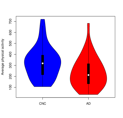
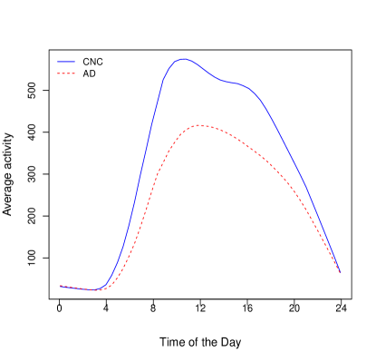
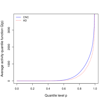
Figure 1: top left: violin plot of subject-specific averages for CNC and AD participants. top right: smoothed diurnal activity profiles averaged across CNC (blue) and AD (red) participants. Bottomleft: average quantile functions of physical activity for AD and CNC participants.

We observe that participants with AD on average, have a lower mean physical activity level compared to CNC. There is also a significant overlap between the two distributions and they are not clearly separable using this PA metric. To formally model this, a generalized linear model (GLM) can be used

$$E(Y_{i}|\bar{X}_{i})=\mu_{i},\hskip 5.69054ptg(\mu_{i})=\alpha+\mathbf{Z}_{i}^{T}\bm{\gamma}+\bar{X}_{i}\beta,$$ (1)

where a scalar regression coefficient $\beta$ represents the effect of average PA on the mean of the response of interest $Y_{i}$ adjusted for covariates $\mathbf{Z}_{i}$ and $g(\cdot)$ is a known link function (e.g., $logit$ or identity).

3.2 Functional data analysis of subject-specific temporal curves

Functional data analysis (FDA) allows us to model temporal aspects in wearable observations $X_{ij}(t)$. To derive subject-specific diurnal minute-level curves, one may average wearable observations across all days at each time-point $t=1,2,\ldots,1440$ as $X_{i}(t)=\frac{1}{n_{i}}\sum_{j=1}^{n_{i}}X_{ij}(t)$. The top right panel of Figure 1 displays average smoothed diurnal activity profiles for CNC (blue) and AD (red) groups. It can be noticed that the curve for mild-AD group have a unimodal diurnal shape, compared to a bimodal shape for CNC, and the largest difference between the two groups appears to be in the morning and in the afternoon (during the second peak for CNC). Similar observations were also made by Varma and Watts ⁷ during their analysis of this data. To formally model the association with functional predictors, scalar-on-function regression (SOFR)¹⁶ can be used as follows

$$E(Y_{i}|X_{i}(t))=\mu_{i},\hskip 5.69054ptg(\mu_{i})=\alpha+\mathbf{Z}_{i}^{T}\bm{\gamma}+\int_{T}X_{i}(t)\beta(t)dt,$$ (2)

where the functional regression coefficient $\beta(t)$ captures the time-varying effect of the diurnal curve $X_{i}(t)$ on the response $Y_{i}$ and $T=(0,24)$ is the daily 24 hour window. Note that, the average subject-specific PA can be estimated back from the diurnal profile $X_{i}(t)$ as $\bar{X}_{i}=\int_{T}X_{i}(t)dt$, therefore for a constant functional regression coefficient $\beta(t)=\beta$, one gets back the generalized linear model (1) for scalar predictors from model (2).

3.3 Distributional data analysis using subject-specific quantile functions

Distributional data analysis can capture and model distributional aspect of wearable observations via subject-specific pdfs, CDFs, or quantile functions ²⁰. If we ignore the temporal information by suppressing the time index $t$, we can denote by $X_{ik}$, $k=1,\ldots,m_{i}$, all wearable observations for subject $i$. We assume $X_{ik}$ follow the same subject-specific distribution defined by subject-specific cumulative distribution function $F_{i}(x)$, where $F_{i}(x)=P(X_{ik}\leq x)$. Then, we can define the subject-specific quantile function $Q_{i}(p)=\inf\{x:F_{i}(x)\geq p\}$. The subject-specific quantile function characterizes the distribution of wearable observations for a specific subject. The subject-specific cdf can be estimated via its empirical counterpart $\hat{F}_{i}(x)=\frac{1}{m_{i}}\sum_{k=1}^{m_{i}}I(X_{ik}\leq x)$ and subject-specific quantile function can be estimated as $\hat{Q}_{i}(p)=\hat{F}_{i}^{-1}(p)$. In this paper, we use the following estimator of quantile functions via a linear interpolation of the order statistics ⁴²:

$$\hat{Q}(p)=(1-w)X_{([(n+1)p])}+wX_{([(n+1)p]+1)},$$

where $X_{(1)}\leq X_{(2)}\leq\ldots,X_{(n)}$ are the corresponding order statistics from a sample $(X_{1},X_{2},\ldots,X_{n})$ and $w$ is a weight satisfying $(n+1)p=[(n+1)p]+w$. Note that the subject-specific average of wearable observations $X_{ij}(t)$ can be also estimated from the subject-specific quantile function as $\bar{X}_{i}=\int_{0}^{1}{Q}_{i}(p)dp$.

The bottom left panel of Figure 1 displays the average quantile functions of physical activity for the CNC and AD groups. A reduced capacity of physical activity can be observed for the AD samples compared to CNC across upper quantile levels such as $p>0.75$. Following the approach of Ghosal et al. ²⁰, the subject-specific quantile functions of PA can be used for modelling $Y_{i}$ using scalar-on-function regression (SOFR) (3) adjusted for $\mathbf{Z}_{i}$. SOFR model is as follows

$$E(Y_{i}|Q_{i}(p))=\mu_{i},\hskip 5.69054ptg(\mu_{i})=\alpha+\mathbf{Z}_{i}^{T}\bm{\gamma}+\int_{0}^{1}Q_{i}(p)\beta(p)dp,$$ (3)

where the functional regression coefficient $\beta(p)$ captures the distributional effect of the PA quantile function $Q_{i}(p)$ on the response of interest $Y_{i}$. In the case $\beta(p)=\beta$, a constant, one again get back the generalized linear model (1) from model (3), since $\bar{X}_{i}=\int_{0}^{1}Q_{i}(p)dp$.

Ghosal et al. ²⁰ re-represented SOFR model for quantile function predictors via L-moments ²⁸. L-moments are defined as the expectation of a linear combination of order statistics. In particular, the $r$-th order L-moment of a random variable $X$ is defined as

$$L_{r}=r^{-1}\sum_{k=0}^{r-1}(-1)^{k}{r-1\choose k}E(X_{r-k:r})\hskip 8.53581ptr=1,2,\ldots,$$

where $X_{1:n}\leq X_{2:n}\leq\ldots\leq X_{n:n}$ denote the order statistics of a random sample of size $n$ drawn from the distribution of $X$. The first order L-moment, $L_{1}$, equals the traditional mean. The second order L-moment, $L_{2}=1/2E(X_{2:2}-X_{1:2})$, represents a robust measure of scale, and equals exactly a half of Gini-coefficient or mean absolute difference. The third and fourth order L-moments, $L_{3}=1/3E(X_{3:3}-2X_{2:3}+X_{1:3})$ and $L_{4}=1/4E(X_{4:4}-3X_{3:4}+3X_{2:4}-X_{1:4})$, capture higher-order distributional properties and normalized by $L_{2}$ can be interpreted similarly to traditional higher-order moments such as skewness and kurtosis. The main advantages of L-moments is the existence of all moments, if first moment exist, their uniqueness and robustness. For SOFR Ghosal et al. ²⁰ adapted an alternative representation of L-moments as projections of quantile functions on Legendre polynomial basis, given by

$$L_{r}=\int_{0}^{1}Q(p)P_{r-1}(p)dp.$$

Here $P_{r}(p)$ is the shifted Legendre polynomial (LP) of degree $r$ defined as

$$P_{r}(p)=\sum_{k=0}^{r}s_{r,k}p^{r},\quad s_{r,k}=(-1)^{r-k}{r\choose k}{r+k\choose k}=\frac{(-1)^{r-k}(r+k)!}{(k!)^{2}(r-k)!}.$$

The shifted Legendre polynomials form an orthogonal basis of $L_{2}[0,1]$. Using the LP decomposition for subject-specific quantile functions $Q_{i}(p)\approx\sum_{k=1}^{K}(2k-1)L_{ik}P_{k-1}(p)$ and $\beta(p)=\sum_{k=1}^{K}\beta_{k}P_{k-1}(p)$, SOFR model can be reduced to a GLM as $g(\mu_{i})=\alpha+\mathbf{Z}_{i}^{T}\bm{\gamma}+\int_{0}^{1}Q_{i}(p)\beta(p)dp=\alpha+\mathbf{Z}_{i}^{T}\bm{\gamma}+\sum_{k=1}^{K}\beta_{k}L_{ik}$. This representation of SOFR via L-moments provides both the functional interpretation of significance of $Q_{i}(p)$ via $\beta(p)$ and the distributional interpretation in terms of the significance of specific L-moments via $\beta_{k}$.

4 Scalar on time-by-distribution regression

In this section, we propose to capture temporally local distributional information in wearable observations using subject-specific time-by-distribution data objects. We develop scalar on time-by-distribution regression (SOTDR) and show how two-way TD data objects can be parsimoniously represented via a collection of time-varying L-moments that capture distributional changes over the time-of-day.

4.1 SOTDR via time-by-distribution data objects

We propose quantile-based time-by-distribution data objects that capture the temporally local distributional aspects of wearable observations. The quantile-based time-by-distribution data object is then defined as

$$Q_{i}(t,p)=\textit{p-th quantile of \{$X_{ij}(s)\}_{j=1}^{n_{i}}$, $s\in(t-h,t+h)$}.$$

Here $2h$ is the window length around time $t$. Note that $Q_{i}(t,p)$ is a bivariate functional summary of subject-specific observational data. For each fixed $t$ (time of the day), it provides distributional encoding as a function of quantile-level $p$, e.g., $Q_{i}(t,\cdot)$ is a quantile function for each $t$. For each fixed $p$, $Q_{i}(\cdot,p)$ captures the diurnal pattern of the $p$-th quantile level of wearable observations as a function of time $t$. Note that the subject-specific average PA can be again be estimated back aggregating the bivariate time-by-distribution data objects as $\bar{X}_{i}=\int_{T}\int_{0}^{1}{Q}_{i}(t,p)dpdt$. For the analysis presented in this paper, we fix total window length $2h=10$ minutes (i.e., $h=5$), but any other window lengths can be used as well. Since the sample considered in this study is highly sedentary ⁸, a window length of 10 minutes still retains the diurnal patterns of PA without any significant loss of information.

Figure 2 displays the heatmaps of average time-by-distribution surfaces $Q_{i}(t,p)$ for CNC (top left) and AD (top right), the difference between them (bottomleft). One can see that the largest differences between the two groups exist during the morning (8 a.m-11 a.m) and in afternoon (3 p.m-5 p.m) across the upper quantile levels ($p>0.6$). At the bottomright panel of Figure 2 we plot the heatmap of difference in time-by-distribution surfaces $Q_{i}(t,p)$ between the participants with high (above $75\%$-percentile) and low (below $25\%$-percentile) cognitive score of attention (ATTN). Overall, TD encoding of physical activity is clearly more informative than just temporal or just distributional information from Figure 1.

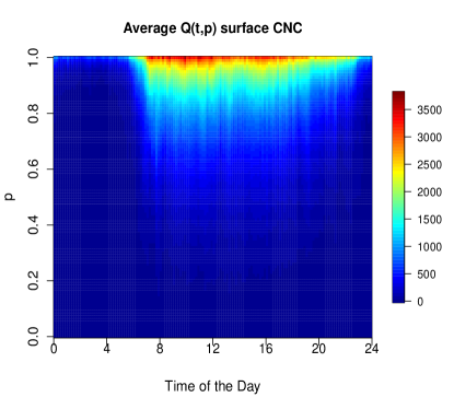
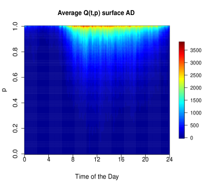
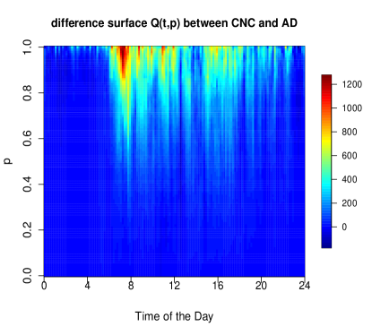
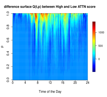
Figure 2: The average bivariate time-by-distribution PA surface $Q_{i}(t,p)$ for CNC (top left) and AD (top right) groups. The difference between CNC and AD (bottomleft) and the difference between subjects with high (above $75\%$ percentile) and low (below $25\%$-percentile) of cognitive attention (ATTN) scores (bottomright).

To formally model the association of TD data objects with scalar response, we propose to use them as predictors in two-way scalar-on-function regression (SOFR) as follows:

$$E(Y_{i}|Q_{i}(t,p))=\mu_{i},\hskip 5.69054ptg(\mu_{i})=\alpha+\mathbf{Z}_{i}^{T}\bm{\gamma}+\int_{0}^{1}\int_{T}Q_{i}(t,p)\beta(t,p)dtdp.$$ (4)

Here $\beta(t,p)$ represents the bivariate functional regression coefficient that captures both the temporal and distributional effect of $Q_{i}(t,p)$ on the response of interest $Y_{i}$. As before, with the constant regression $\beta(t,p)=\beta$, the bivariate SOFR model (4) reduces to the generalized linear model (1) for scalar predictors. The estimation approach of this model is discussed below.

Estimation of the time-by-distribution regression coefficient $\beta(t,p)$

We follow a two-step estimation approach for the bivariate SOFR model (4) in the paper. In step 1, we model the bivariate regression functional coefficient $\beta(t,p)$ using a tensor product of univariate cubic B-spline basis functions of both temporal and quantile level arguments, $t$ and $p$. Suppose, $\{B_{T,k}(t)\}^{K_{0}}_{k=1}$ and $\{B_{P,\ell}(p)\}^{L_{0}}_{\ell=1}$ are the set of known basis functions over $t$ and $p$, respectively. Then, $\beta(t,p)$ is modelled as $\beta(t,p)=\sum_{k=1}^{K_{0}}\sum_{\ell=1}^{L_{0}}\theta_{k,\ell}B_{T,k}(t)B_{P,\ell}(p)$. Using this expansion model (4) is reformulated as

$$g(\mu_{i}) = \alpha+\mathbf{Z}_{i}^{T}\bm{\gamma}+\sum_{k=1}^{K_{0}}\sum_{\ell=1}^{L_{0}}\theta_{k,\ell}\int_{T}\int_{0}^{1}Q_{i}(t,p)B_{T,k}(t)B_{P,\ell}(p)dtdp$$ (5)

$$= \alpha+\mathbf{Z}_{i}^{T}\bm{\gamma}+\mathbf{W}_{i}^{T}\bm{\theta},$$

where we denote by $\mathbf{W}_{i}$ the $K_{0}L_{0}$-dimensional stacked vectors of $\{\int_{0}^{1}Q_{i}(t,p)B_{T,k}(t)B_{P,\ell}(p)dtdp\}_{k=1,\ell=1}^{K_{0},L_{0}}$ and $\bm{\theta}$ is the corresponding $K_{0}L_{0}$-dimensional vector of unknown basis coefficients $\theta_{k,\ell}$’s. Thus, the model (5) can be seen as a GLM with subject specific predictors $\mathbf{W}_{i}^{k,\ell}=\int_{0}^{1}Q_{i}(t,p)B_{T,k}(t)B_{P,\ell}(p)dtdp$. We use a penalized negative log-likelihood criterion with LASSO ⁴³ penalty on the coefficients, which simultaneously identifies the most informative time of the day and the quantile levels. This effectively helps to reduce the number of parameters (variables) in the model and allows a sparse representation of the functional regression coefficient $\beta(t,p)$, which is, especially, important when dealing with a relatively small sample size such as in our motivating application with $n=92$. The penalized negative log likelihood criterion is given by

$$S(\psi)=R(\alpha,\bm{\gamma},\bm{\theta})=-2logL(\alpha,\bm{\gamma},\bm{\theta};Y_{i},\mathbf{Z}_{i},\mathbf{W}_{i})+||\bm{\theta}||_{1}.$$ (6)

In step 2, the selected predictors $\mathbf{W}_{i}^{k,\ell}$ (with non-zero coefficients) are used in the GLM (5) without any penalization (this also overcomes penalization bias of LASSO) for inference. The estimated regression coefficient function is then given by $\hat{\beta}(t,p)=\sum_{k=1}^{K_{0}}\sum_{\ell=1}^{L_{0}}\hat{\theta}_{k,\ell}B_{T,k}(t)B_{P,\ell}(p)$ (note that $\hat{\theta}_{k,\ell}=0$ if $\mathbf{W}_{i}^{k,\ell}$ is not selected in the first step).

4.2 SOTDR-L: SOTDR via time-varying L-moments

Following Ghosal et al. ²⁰ who adapted L-moments to SOFR with quantile function predictors, we adapt L-moments to SOTDR by introducing subject-specific time-varying L-moments $L_{ir}(t)$ that depend on the time of the day $t$. Specifically, we define the diurnal time-varying $r$-th order L-moment for subject $i$ as

$$L_{ir}(t)=\textit{r-th L-moment of \{$X_{ij}(s)\}_{j=1}^{n_{i}}$, $s\in(t-h,t+h)$}.$$

Here we again consider a window of total length $2h$ centered at time $t$. The diurnal time-varying $L_{ir}(t)$ curves capture the temporal change of the subject-specific distribution. For example, the first order time-varying L-moment $L_{i1}(t)$ simply represents the diurnal mean curve $X_{i}(t)$ aggregated into 10 minutes epoch (for $h=5$). The second order time-varying L-moment $L_{i2}(t)$ captures a temporal change in variability and is similar to the diurnal standard deviation curve of physical activity considered by Varma and Watts ⁷.

Figure 3 displays the first four time-varying L-moments $L_{r}(t)$ of physical activity, averaged within CNC (blue) and AD (red) groups. Note that the first time-varying L-moments $L_{1}(t)$ exactly equal to the temporal diurnal curves from the top right panel of Figure 1. Subject-specific $r$-th order time-varying L-moment $L_{ir}(t)$ is related to the time-by-distribution PA data object $Q_{i}(t,p)$ through its projection on Legendre polynomial basis $P_{r-1}(p)$ as follows

$$L_{ir}(t)=\int_{0}^{1}Q_{i}(t,p)P_{r-1}(p)dp.$$

One can notice that mild AD have lower $L_{1}(t)$, $L_{2}(t)$, $L_{3}(t)$, and $L_{4}(t)$ moments compared to the CNC, particularly in the morning and somewhat in the afternoon.

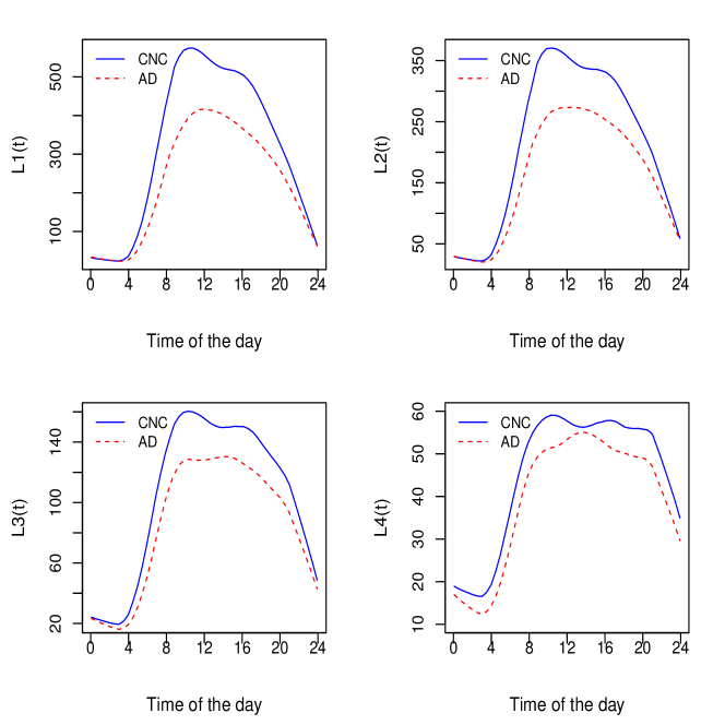
Figure 3: The first four time-varying L-moments of daily physical activity averaged within CNC (blue) and AD (red) groups.

We propose to use the time-varying subject-specific L-moments $L_{ir}(t)$ for modelling $Y_{i}$ using an additive SOFR model. If the shifted Legendre polynomials $P_{\ell-1}(p)$ are used as the basis in $p$ for modelling the bivariate functional effect $\beta(t,p)$, the additive SOFR model (7) in terms of time-varying L-moments of PA provides an alternative representation of the bivariate SOFR model (4) that is additionally interpretable from distributional point of view. We will refer to this approach as SOTDR-L. In particular, we have,

$$g(\mu_{i}) =\alpha+\mathbf{Z}_{i}^{T}\bm{\gamma}+\int_{0}^{1}\int_{T}Q_{i}(t,p)\beta(t,p)dtdp$$

$$=\alpha+\mathbf{Z}_{i}^{T}\bm{\gamma}+\int_{T}\sum_{k=1}^{K_{0}}\sum_{\ell=1}^{L_{0}}\theta_{k,\ell}B_{T,k}(t)\int_{0}^{1}Q_{i}(t,p)P_{\ell-1}(p)dtdp$$

$$=\alpha+\mathbf{Z}_{i}^{T}\bm{\gamma}+\sum_{\ell=1}^{L_{0}}\int_{T}L_{i\ell}(t)\sum_{k=1}^{K_{0}}\theta_{k,\ell}B_{T,k}(t)dt$$

$$=\alpha+\mathbf{Z}_{i}^{T}\bm{\gamma}+\sum_{\ell=1}^{L_{0}}\int_{T}L_{i\ell}(t)\beta_{\ell}^{*}(t)dt.$$ (7)

Here the functional regression coefficient $\beta^{*}_{r}(t)$ capture the diurnal time-varying effect of the $r$-th order time-varying L-moment on the response $Y_{i}$ at time $t$. Thus, we get an additive SOFR with time-varying L-moments. It is important to note that if $L_{0}=1$ we get exactly the SOFR model (2) that uses subject-specific temporal curves as predictors. Thus, SODTR-L model (7) strictly includes model (2).

5 Application of SOTDR to modelling cognitive status and function in Alzheimer’s Disease

In this section, we apply SOTDR to model cognitive status and function in the Alzheimer’s disease (AD) study and compare it to the three existing approaches including regression via scalar summaries, SOFR with temporal diurnal curves, SOFR with quantile functions. The refund package ⁴⁴ in R ⁴⁵ is used for implementation of SOFR. First, we will model cognitive status (CNC vs AD) and the three cognitive scores of attention (ATTN), visual memory (VM), and executive function (EF) using the bivariate time-by-distribution data objects as illustrated in the Section 4.1. Second, we alternatively use an additive SOFR with time-varying L-moments.

5.1 SOTDR modelling of cognitive status

We model cognitive status (CNC vs AD) using the SODTR model (4) with an additive adjustment for age, sex and years of education. For comparison with existing approaches, we fit models (1), (2) and (3) using as predictors subject-specific average PA, diurnal PA curves, quantile PA functions, respectively. Ten minute diurnal PA curves have been calculated by aggregating minute-level data into 10 minutes epochs, resulting in subject-specific diurnal PA curves $X_{i}(t)$ of length $144$. As mentioned earlier, since the participants of the study were highly sedentary ⁸ such 10-minute aggregation serves as pre-smoothing and retains the key temporal patterns of PA. When we report predictive performance summaries such as area under the curve (AUC) of the receiver operating characteristic, we perform repeated cross-validation and report the average cross-validated AUC (cvAUC). The results of the analyses are presented in Table 2.

Table 2: The results of modelling cognitive status (CNC vs AD) and physical activity using Model 1-4 with an adjustment for age, sex, and education. The standard deviation of the estimated coefficients for the scalar predictors are indicated in the parenthesis. Predictors: model 1-scalar average PA, model 2- diurnal PA curves, model 3 - quantile functions, model 4 - SOTDR with time-by-distribution data objects.

	Dependent variable : Cognitive Status (CNC vs AD)
	Model 1	Model 2	Model 3	Model 4
Intercept	7.608∗∗	6.549∗	10.588∗∗	12.368∗∗∗
	(3.567)	(3.615)	(4.139)	(4.591)
age	$-$0.051	$-$0.040	$-0.072^{*}$	$-0.089^{*}$
	(0.038)	(0.039)	(0.043)	(0.047)
sex	2.134∗∗∗	2.111∗∗∗	2.527∗∗∗	2.637∗∗∗
	(0.554)	(0.553)	(0.624)	(0.676)
education	$-$0.224∗∗	$-$0.213∗∗	$-$0.167∗	$-$0.174∗
	(0.091)	(0.091)	(0.092)	(0.095)
$\bar{X}_{i}$	$-$0.005∗∗∗	NA	NA	NA
	(0.002)
$X_{i}(t)$	NA	$\hat{\beta}(t)^{**}$	NA	NA
$Q_{i}(p)$	NA	NA	$\hat{\beta}(p)^{**}$	NA
$Q_{i}(t,p)$	NA	NA	NA	$\hat{\beta}(t,p)^{***}$
Observations	92	92	92	92
cvAUC	0.781	0.773	0.792	0.811
Note:	∗p$<$0.1; ∗∗p$<$0.05; ∗∗∗p$<$0.01

Model 1 shows that higher subject-specific average PA is significantly associated ($\alpha$= $0.05$) with a lower odds of AD. The cvAUC value of 0.781 illustrates a satisfactory discriminatory power of the model and is set as a benchmark for comparison with the other three models. The estimated functional regression coefficient $\beta(t)$ for Model 2 illustrating a diurnal effect of PA profile on log-odds of AD is displayed in the top left panel of Figure 4. Model 2 finds that higher PA during morning hours ($\sim$ 10 am-3 p.m) is significantly associated ($\alpha=0.05$) with a lower odds of AD ⁴⁶.

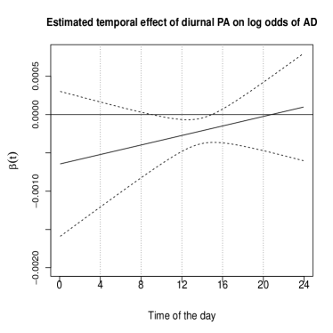
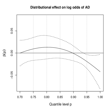
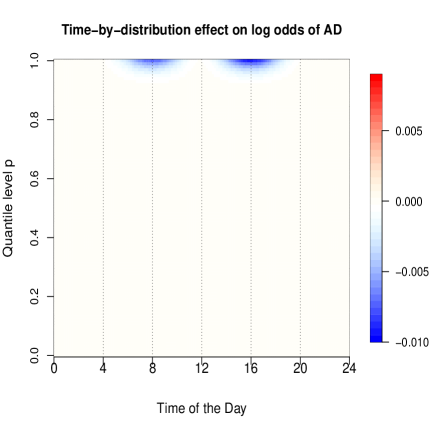
Figure 4: The estimated regression coefficients for Models 2-4. Estimated temporal effect $\beta(t)$ (top left. $t$ denoting time of the day). Estimated distributional effect $\beta(p)$ (top right, $p\in(0.7,1)$). Estimated bivariate effect $\beta(t,p)$ of time-by-distribution PA surface (bottomleft).

The average cvAUC of $0.773$ suggests that, although, the diurnal patterns of average PA offer additional temporal insights, they do not necessarily offer more discrimination between CNC and AD group compared to the use of simple average PA (Model 1, cvAUC = $0.781$). Model 3 finds the significance of subject-specific quantile functions of PA. The estimated functional regression coefficient $\beta(p)$ for Model 3 illustrating a distributional effect of PA on log-odds of AD is displayed ($\beta(p)$ not significant for $p<0.7$) in the top right panel of Figure 4 and shows that higher upper quantile levels ($p\in(0.90,1)$) of PA are significantly associated with lower odds of AD ⁴⁶. Increased cvAUC of $0.792$ indicates higher discriminatory power of distributional encoding of PA (in particular, maximal PA) between CNC and AD compared to the average PA.

The estimated bivariate functional effect $\beta(t,p)$ for Model 4 is shown in the bottomleft panel of Figure 4. We used $K_{0}=L_{0}=12$ cubic B-spline basis functions for modelling $\beta(t,p)$. Increased maximal capacity of PA during the morning ($\sim$ 7 a.m- 10 a.m) and in the afternoon ($\sim$ 3 p.m- 5 p.m) is found to be associated with lower odds of AD. An increased cvAUC of $0.811$ (around 3.8 $\%$ gain) illustrates additional discriminatory power of the time-by-distribution PA data objects, while simultaneously capturing temporally local distributional effects of the PA on log-odds of AD.

5.2 SOTDR-L modelling of cognitive status

Next, we illustrate an application of SOTDR-L that uses diurnal time-varying L-moments for modelling cognitive status (CNC vs AD) outcome. For interpretability, we use the first four diurnal L-moments profile $L_{ik}(t)$ ($L_{0}=4$) as functional predictors and adjust for age, sex and years of education. Since we have a relatively small sample size (n=92), we follow a penalized SOFR approach

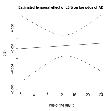
Figure 5: Estimated diurnal effect $\beta(t)$ of $L_{i3}(t)$ of PA on log odds of AD.

to select the L-moments $L_{ik}(t)$-s, which are most informative. In particular, we re-express the SOFR model (7) in terms of functional principal component scores of $L_{ik}(t)$ following a functional principal component regression approach ⁴⁷, ⁴⁸,

$$E(Y_{i}|\{L_{ir}(t)\}_{r=1}^{4})=\mu_{i},\hskip 5.69054ptg(\mu_{i})=\alpha+\mathbf{Z}_{i}^{T}\bm{\gamma}+\sum_{r=1}^{4}\sum_{s=1}^{n_{r}}\xi_{irs}\beta_{r,s}.$$ (8)

Here $\xi_{irs}=\int_{T}L_{ir}(t)\psi_{s}(t)$ is the projection of the diurnal L-moment $L_{ir}(t)$ on the eigenbasis $\psi_{s}(t)$ and $\beta_{r}(t)$ is modelled as $\beta_{r}(t)=\sum_{s=1}^{n_{r}}\beta_{r,s}\psi_{s}(t)$. We use the group exponential Lasso (GEL) penalty ⁴⁹ on the basis coefficients $\{\beta_{r,s}\}_{s=1}^{n_{r}}$ to perform variable selection in order to identify informative time-varying L-moments $L_{ik}(t)$. GEL is a bi-level selection penalty and enjoys the added flexibility of forcing some of the coefficients within a particular group to be zero, thus effectively reducing the number of parameters, which is especially useful in our scenario due to the very low sample size. The proposed variable selection approach selects the 3rd order time-varying L-moments $L_{i3}(t)$ to be most informative i.e, most discriminating between the two groups (CNC and AD) while adjusting for age, sex and years of education. The grpreg package ⁵⁰ in R is used for implementing the variable selection method using GEL. The estimated diurnal effect of $L_{i3}(t)$ is shown in Figure 5. We observe that an increase in the value of third order L-moment of physical activity, during the window (8 a.m- 6 p.m) is associated with a lower odds of AD. The third order L-moment $L_{i3}(t)$ is related to L-skewness of the PA and its significance is therefore very interesting from a clinical perspective. We also perform repeated cross-validation using $L_{i3}(t)$ as predictor in a SOFR model while adjusting for age, sex, and years of education. An increased cvAUC of $0.802$ (around 2.7 $\%$ gain) illustrates satisfactory discriminatory power of the proposed metric offering both distributional and temporal encoding of physical activity. Likely, because of restricting the number of L-moments and the use of GEL, the temporal findings of SOTDR-L differ from temporal findings of SOTDR. While SOTDR highlights activity in the upper quantile levels during 6-10am and 2-6pm time periods, SOTDR-L highlights the third order L-moment of activity during mid-day hours that are similar to those from SOFR on temporal diurnal curves. Chosen third order time-varying L-moments in SOTDR-L also seems to result in an increase in cvAUC compared to SOFR that uses temporal diurnal curves (that are equivalent to the first order time-varying L-moments).

5.3 Modelling attention

In this section, we apply SOTDR to the cognitive score of attention (ATTN) and the results are compared with those from regression with subject-specific average PA, FDA using diurnal PA curves, DDA using quantile functions. Adjusted R-squared, defined as the adjusted proportion of variance explained, where original variance and residual variance are both estimated using unbiased estimators ⁵¹, is used in Models 2-4 for the evaluation of predictive performance.

Table 3: The results of modelling attention score and physical activity using Model 1-4 with an adjustment for age, sex, and education. The standard deviation of the estimated coefficients for the scalar predictors are indicated in the parenthesis. Predictors: model 1-scalar average PA, model 2- diurnal PA curves, model 3 - quantile functions, model 4 - SOTDR with time-by-distribution data objects. All models are adjusted for age, sex, years of education.

	Dependent variable : ATTN score
	Model 1	Model 2	Model 3	Model 4
Intercept	$-$1.423	$-$1.157	$-2.045^{**}$	-3.696∗∗∗
	(0.929)	(0.960)	(0.927)	(0.988)
age	0.002	-0.001	0.006	$0.021^{*}$
	(0.011)	(0.011)	(0.010)	(0.011)
sex	$-$0.354∗∗	$-$0.349∗∗	$-$0.443∗∗∗	$-0.476^{***}$
	(0.150)	(0.150)	(0.150)	(0.134)
education	0.083∗∗∗	0.080∗∗∗	0.072∗∗∗	$0.069^{***}$
	(0.023)	(0.023)	(0.023)	(0.021)
$\bar{X}_{i}$	0.0005	NA	NA	NA
	(0.0005)
$X_{i}(t)$	NA	$\hat{\beta}(t)$	NA	NA
$Q_{i}(p)$	NA	NA	$\hat{\beta}(p)^{**}$	NA
$Q_{i}(t,p)$	NA	NA	NA	$\hat{\beta}(t,p)^{***}$
Observations	92	92	92	92
Adjusted R2	0.161	0.163	0.218	0.378
Note:	∗p$<$0.1; ∗∗p$<$0.05; ∗∗∗p$<$0.01

Table 3 presents the result of the analyses from these four modelling approaches. The association between average PA and attention is not found to be significant at $\alpha=0.05$ level. Adjusted R-squared of the model is reported to be $0.161$ and is set as the benchmark for comparison with the other approaches. Although, the diurnal curves of PA were not found to be significant ($\alpha=0.05$ level), the estimated quantile-function effect is significant. The estimated regression coefficient $\beta(p)$ is shown in Figure 6 (top right panel). It shows that $\beta(p)$ creates a contrast between a higher quantile levels ($p>0.8$) and lower quantile levels ($p<0.8$). Specifically, an increase in higher quantile of PA is found to be associated with higher performance on attention. Although, one needs to be cautious in interpreting the results as subject- specific quantiles of PA are mostly zero below the quantile level $p<0.5$ as illustrated in Figure 1. A $35\%$ increase in the adjusted R-squared is observed using DDA with subject-specific quantile functions of PA compared to the benchmark model.

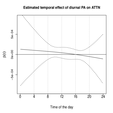
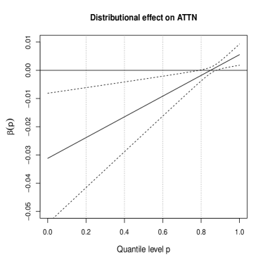
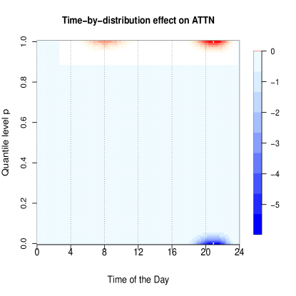
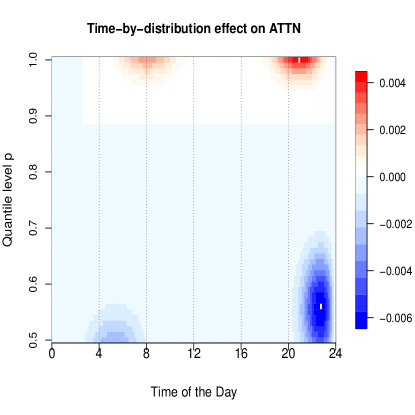
Figure 6: The estimated effects of the different PA metrics (Model 2-4) on ATTN score. Estimated temporal effect (solid line) $\beta(t)$ (top left). Estimated distributional effect $\beta(p)$ (top right). Estimated bivariate effect $\beta(t,p)$ of time-by-distribution PA surface (bottomleft). The same plot with $p$ restricted to the distributional domain $(0.5,1)$ (bottomright).

The estimated bivariate coefficient $\beta(t,p)$, capturing the TD effect on attention is displayed in Figure 6 (bottomleft panel). Increased maximal capacity of PA during the morning ($\sim$ 7 a.m - 10 a.m) and in the evening ($\sim$ 8 p.m - 10 p.m) is found to be associated with higher attention score after adjusting for age, sex and years of education. Importantly, when quantile levels are constrained to be above 0.5 (re-estimated $\beta(t,p)$ is shown in the bottomright), there are two contrasts between upper quantile levels ($p>0.9$) and lower quantile levels ($0.5<p<0.7$) which are not time-aligned and actually capture quantile contrast between adjacent time periods. The morning TD effect can be interpreted as lower level quantile activity centered around 4-6 a.m are negatively associated and higher level quantile activity centered around 7-9 a.m are positively associated with attention. The evening TD effect can be interpreted higher level quantile activity centered around 8-10 p.m are positively associated and lower level quantile activity centered around 10 p.m-12 a.m are negatively associated with with attention. Adjusted R-squared of SOTDR model using the time-by-distribution PA surface is reported to be $0.378$, giving a $135\%$ gain from the benchmark model using average physical activity, demonstrating very strong time-by-distribution effect, compared to the non-significant average and diurnal effect and significant distributional effect. The results from the similar SOTDR analysis of verbal memory (VM) and executive function (EF) are presented in the Supplementary Tables A1, A2 and Supplementary Figures B1, B2 of the Appendix. For both outcomes, we observed significant improvements in adjusted R-squared.

5.4 SOTDR-based scalar biomarkers

Estimated SOTDR can be used to create a simpler to use and interpret scalar biomarkers. For example, based on the previously fitted models for an outcome of interest, one can calculate following SOTDR biomarkers $bm_{TD,i}=\int_{0}^{1}\int_{T}Q_{i}(t,p)\hat{\beta}(t,p)dtdp$ and compare them with the models based on the average PA, diurnal curves of PA, and quantile functions of PA: $bm_{a,i}=\bar{X}_{i}\hat{\beta}$, $bm_{T,i}=\int_{T}X_{i}(t)\hat{\beta}(t)dt$, $bm_{D,i}=\int_{0}^{1}Q_{i}(p)\hat{\beta}(p)dp$. Figure 7 displays the scatterplot matrix for all four types of biomarkers to discriminate either cognitive status (left) and attention score (right). Although, they are mostly positively correlated, the large amount of spread indicates that they likely capture somewhat different aspects of PA.

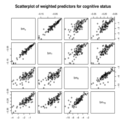
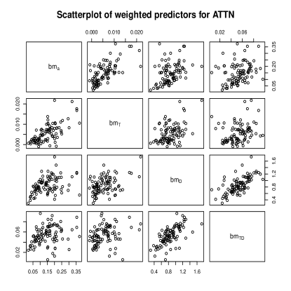
Figure 7: scatterplots of the estimated weighted scores corresponding to the predictors average PA, diurnal PA curve, PA quantile function and time-by-distribution PA metric respectively for cognitive status (left) and ATTN (right).

6 Discussion

In this paper, we have used subject-specific time-by-distribution data objects to capture and model temporally local distributional information in wearable data. We then developed a scalar on time-by-distribution regression that handles TD objects as predictors. We have also provided an alternative and parsimonious representation of the time-by-distribution objects in terms of time-varying L-moments, robust rank-based analogs of traditional moments. This representation allowed us to illustrate that SOTDR generalizes SOFR.

Our approach revealed novel insights in the associations between distributional and diurnal aspects of physical activity and various domains of cognitive function and Alzheimer’s disease status. The time-by-distribution representation provided better discrimination between the CNC and AD participants. Our results revealed strong associations between temporally local distributional aspects of PA across the day and clinical cognitive scales impacted in early AD, especially, attention. These results highlight the potential value of designing and testing physical activity interventions targeting specific time of the day, in the early stages of AD. As there may be times of the day when cognitively impaired individuals are most alert ⁵², ⁵³, it might be specifically suited for individual specific PA interventions. Note that, although we have not established a causal direction here, it could also be that people with AD have poor sleep, so are less active in the morning compared to cognitively normal controls. The maximal capacity of physical activity represents reserve of a individual and our study has revealed strong and significant associations between cognitive performance and maximal PA levels, indicating changes in the reserve of a person might be sensitive to specific disease pathology and cognitive decline.

This paper opens interesting research questions on how to efficiently capture information with TD data objects. In our approach we encoded distributional information via quantile functions, the use of other distributional representation such as CDF or hazard function could be explored in future work. In our application, the window length $h$ for calculating $Q_{i}(t,p)$ and $L_{i}(t)$ was chosen to be consistent with the window size for diurnal curves. However, in other applications, an adaptive procedure of the choice of optimal window size $h$ may be developed. Time registration or time-warping is often a desirable pre-processing step to make sure the amplitude and phase variations in functional data are properly separated ⁵⁴, ⁵⁵, ⁵⁶. This is, especially, important for wearable data which often driven by subject-specific schedules and time preferences. Thus, pre-registration of TD objects is another exciting area of future research. We have focused on a linear effect of the TD data objects in this paper due to it’s simplicity, interpretability and connection with summary level modelling approaches. Accounting for circular nature of the data may be another interesting direction. Future applications might benefit from considering nonlinear effects of the TD objects and this could be done via nonlinear extensions scalar-on-function regression models ¹⁶. Another interesting area of research would be to extend and apply the proposed method for modelling longitudinal data that at each visit generate distribution. For example, this could offer novel insights into the distributional changes in physical activity at different ages across the lifespan. ².

R Vignette

Illustration of the proposed framework via R ⁴⁵, along with the dataset analyzed, is available online with this article and on Github at https://github.com/rahulfrodo/SOTDR.

Conflict of interest

The authors declare no potential conflict of interests.

Supporting information

Supplementary Tables A1, A2 and Supplementary Figures B1, B2 are available as supporting information as part of the online article.

Appendix A Supplementary Tables

Table 4: Results from modelling cognitive score of VM on age, sex, education and physical activity metrics using Model 1-4. The standard deviation of the estimated coefficients for the scalar predictors are indicated in the parenthesis. Model 1: summary level modelling using average PA, Model 2: Temporal modelling using diurnal PA, Model 3: Distributional modelling using PA quantile function, Model 4: Joint modelling using PA time-by-distribution bivariate surface.

	Dependent variable : VM score
	Model 1	Model 2	Model 3	Model 4
Intercept	$-$2.329	$-$1.561	$-3.635^{*}$	-3.786∗
	(1.950)	(2.006)	(1.948)	(2.061)
age	$-$0.009	$-$0.017	0.001	$-0.0001$
	(0.023)	(0.023)	(0.022)	(0.023)
Sex	$-$1.355∗∗∗	$-$1.338∗∗∗	$-$1.533∗∗∗	$-1.35^{***}$
	(0.315)	(0.313)	(0.312)	(0.306)
education	0.164∗∗∗	0.156∗∗∗	0.142∗∗∗	$0.126^{***}$
	(0.049)	(0.049)	(0.048)	(0.047)
$\bar{X}_{i}$	0.003∗∗∗	NA	NA	NA
	(0.001)
$X_{i}(t)$	NA	$\hat{\beta}(t)^{***}$	NA	NA
$Q_{i}(p)$	NA	NA	$\hat{\beta}(p)^{***}$	NA
$Q_{i}(t,p)$	NA	NA	NA	$\hat{\beta}(t,p)^{***}$
Observations	92	92	92	92
Adjusted R2	0.331	0.338	0.375	0.413
Note:	∗p$<$0.1; ∗∗p$<$0.05; ∗∗∗p$<$0.01

Table 5: Results from modelling cognitive score of EF on age, sex, education and physical activity metrics using Model 1-4. The standard deviation of the estimated coefficients for the scalar predictors are indicated in the parenthesis. Model 1: summary level modelling using average PA, Model 2: Temporal modelling using diurnal PA, Model 3: Distributional modelling using PA quantile function, Model 4: Joint modelling using PA time-by-distribution bivariate surface.

	Dependent variable : EF score
	Model 1	Model 2	Model 3	Model 4
Intercept	$-$2.479	$-$1.944	$-3.070^{**}$	$-$3.760∗∗
	(1.492)	(1.539)	(1.531)	(1.612)
age	$-$0.0002	$-$0.006	$0.004$	0.009
	(0.017)	(0.018)	(0.017)	(0.018)
Sex	$-$1.063∗∗∗	$-$1.051∗∗∗	$-$1.141∗∗∗	$-1.094^{***}$
	(0.241)	(0.240)	(0.245)	(0.230)
education	0.141∗∗∗	0.136∗∗∗	0.132∗∗∗	$0.116^{***}$
	(0.037)	(0.037)	(0.038)	(0.036)
$\bar{X}_{i}$	0.002∗∗∗	NA	NA	NA
	(0.001)
$X_{i}(t)$	NA	$\hat{\beta}(t)^{***}$	NA	NA
$Q_{i}(p)$	NA	NA	$\hat{\beta}(p)^{***}$	NA
$Q_{i}(t,p)$	NA	NA	NA	$\hat{\beta}(t,p)^{***}$
Observations	92	92	92	92
Adjusted R2	0.337	0.341	0.347	0.411
Note:	∗p$<$0.1; ∗∗p$<$0.05; ∗∗∗p$<$0.01

Appendix B Supplementary Figures

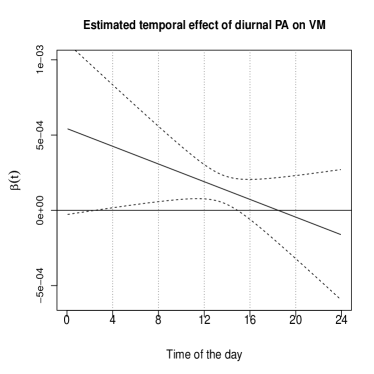
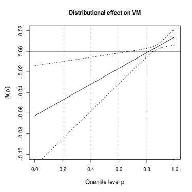
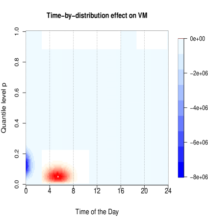
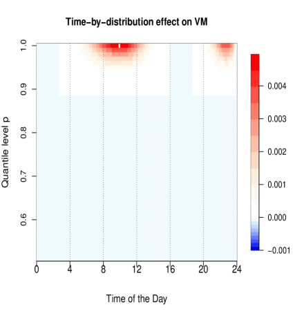
Figure 8: The estimated effects of the different PA metrics (Model 2-4) on VM score. Estimated temporal effect (solid line) $\beta(t)$ (top left). Estimated distributional effect $\beta(p)$ (top right). Estimated bivariate effect $\beta(t,p)$ of time-by-distribution PA surface (bottomleft). The same plot with $p$ restricted to $(0.5,1)$ (bottomright). Higher maximal PA during the morning and night are found be associated with a higher score of VM. Higher minimal PA during early morning also appears to be associated with higher score of VM, caution should be taken when interpreting the results for $p<0.5$.

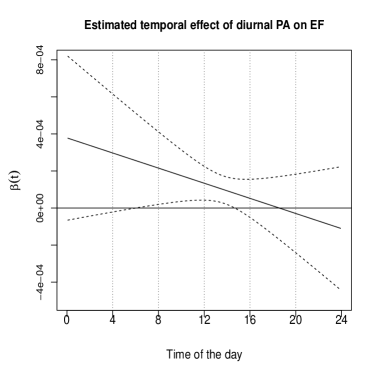
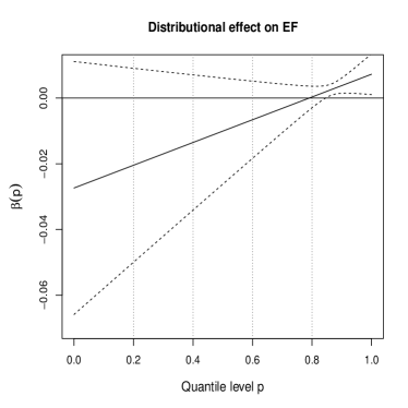
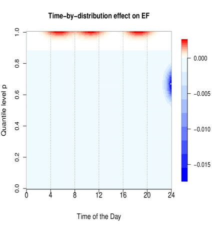
Figure 9: The estimated effects of the different PA metrics (Model 2-4) on EF score. Estimated temporal effect (solid line) $\beta(t)$ (top left). Estimated distributional effect $\beta(p)$ (top right). Estimated bivariate effect $\beta(t,p)$ of time-by-distribution PA surface (bottomleft). Higher maximal PA during the morning and evening is found to be associated with higher EF score.

References

- 1 Karas M, Bai J, Strączkiewicz M, et al. Accelerometry data in health research: challenges and opportunities. Statistics in biosciences 2019; 11(2): 210–237.
- 2 Varma VR, Dey D, Leroux A, et al. Re-evaluating the effect of age on physical activity over the lifespan. Preventive medicine 2017; 101: 102–108.
- 3 Schrack JA, Zipunnikov V, Goldsmith J, et al. Assessing the “physical cliff”: detailed quantification of age-related differences in daily patterns of physical activity. Journals of Gerontology Series A: Biomedical Sciences and Medical Sciences 2014; 69(8): 973–979.
- 4 Xiao L, Huang L, Schrack JA, Ferrucci L, Zipunnikov V, Crainiceanu CM. Quantifying the lifetime circadian rhythm of physical activity: a covariate-dependent functional approach. Biostatistics 2015; 16(2): 352–367.
- 5 Urbanek JK, Zipunnikov V, Harris T, Crainiceanu C, Harezlak J, Glynn NW. Validation of gait characteristics extracted from raw accelerometry during walking against measures of physical function, mobility, fatigability, and fitness. The Journals of Gerontology: Series A 2018; 73(5): 676–681.
- 6 Varma VR, Ghosal R, Hillel I, et al. Continuous gait monitoring discriminates community-dwelling mild Alzheimer’s disease from cognitively normal controls. Alzheimer’s & Dementia: Translational Research & Clinical Interventions 2021; 7(1): e12131.
- 7 Varma VR, Watts A. Daily physical activity patterns during the early stage of Alzheimer’s disease. Journal of Alzheimer’s Disease 2017; 55(2): 659–667.
- 8 Watts A, Walters RW, Hoffman L, Templin J. Intra-individual variability of physical activity in older adults with and without mild Alzheimer’s disease. PLoS One 2016; 11(4): e0153898.
- 9 Bakrania K, Yates T, Edwardson CL, et al. Associations of moderate-to-vigorous-intensity physical activity and body mass index with glycated haemoglobin within the general population: a cross-sectional analysis of the 2008 Health Survey for England. BMJ open 2017; 7(4): e014456.
- 10 Di J, Leroux A, Urbanek J, et al. Patterns of sedentary and active time accumulation are associated with mortality in US adults: The NHANES study. bioRxiv 2017: 182337.
- 11 Schrack JA, Kuo PL, Wanigatunga AA, et al. Active-to-sedentary behavior transitions, fatigability, and physical functioning in older adults. The Journals of Gerontology: Series A 2019; 74(4): 560–567.
- 12 Morris JS, Arroyo C, Coull BA, Ryan LM, Herrick R, Gortmaker SL. Using wavelet-based functional mixed models to characterize population heterogeneity in accelerometer profiles: a case study. Journal of the American Statistical Association 2006; 101(476): 1352–1364.
- 13 Goldsmith J, Liu X, Jacobson J, Rundle A. New insights into activity patterns in children, found using functional data analyses. Medicine and science in sports and exercise 2016; 48(9): 1723.
- 14 Cui E, Crainiceanu CM, Leroux A. Additive Functional Cox Model. Journal of Computational and Graphical Statistics 2020: 1–14.
- 15 Goldsmith J, Zipunnikov V, Schrack J. Generalized multilevel function-on-scalar regression and principal component analysis. Biometrics 2015; 71(2): 344–353.
- 16 Reiss PT, Goldsmith J, Shang HL, Ogden RT. Methods for scalar-on-function regression. International Statistical Review 2017; 85(2): 228–249.
- 17 Leroux A, Di J, Smirnova E, et al. Organizing and analyzing the activity data in NHANES. Statistics in biosciences 2019; 11(2): 262–287.
- 18 Augustin NH, Mattocks C, Faraway JJ, Greven S, Ness AR. Modelling a response as a function of high-frequency count data: The association between physical activity and fat mass. Statistical methods in medical research 2017; 26(5): 2210–2226.
- 19 Yang H, Baladandayuthapani V, Rao AU, Morris JS. Quantile function on scalar regression analysis for distributional data. Journal of the American Statistical Association 2020; 115(529): 90–106.
- 20 Ghosal R, Varma VR, Volfson D, et al. Distributional data analysis via quantile functions and its application to modelling digital biomarkers of gait in Alzheimer’s Disease. arXiv 2021.
- 21 Matabuena M, Petersen A. Distributional data analysis with accelerometer data in a NHANES database with nonparametric survey regression models. arXiv 2021.
- 22 Kokoszka P, Miao H, Petersen A, Shang HL. Forecasting of density functions with an application to cross-sectional and intraday returns. International Journal of Forecasting 2019; 35(4): 1304–1317.
- 23 Tang B, Zhao Y, Venkataraman A, et al. Differences in functional connectivity distribution after transcranial direct-current stimulation: a connectivity density point of view. bioRxiv 2020.
- 24 Matabuena M, Petersen A, Vidal JC, Gude F. Glucodensities: a new representation of glucose profiles using distributional data analysis. Statistical Methods in Medical Research. 2021.
- 25 Horváth L, Kokoszka P, Wang S. Monitoring for a change point in a sequence of distributions. Annals of Statistics 2020.
- 26 Sharma A, Gerig G. Trajectories from Distribution-Valued Functional Curves: A Unified Wasserstein Framework. In: Springer. ; 2020: 343–353.
- 27 Marx BD, Eilers PH. Multidimensional penalized signal regression. Technometrics 2005; 47(1): 13–22.
- 28 Hosking JR. L-moments: Analysis and estimation of distributions using linear combinations of order statistics. Journal of the Royal Statistical Society: Series B (Methodological) 1990; 52(1): 105–124.
- 29 Gronek P, Balko S, Gronek J, et al. Physical Activity and Alzheimer’s Disease: A Narrative Review. Aging and disease 2019; 10(6): 1282.
- 30 Zvěřová M. Alzheimer’s disease and blood-based biomarkers–potential contexts of use. Neuropsychiatric disease and treatment 2018; 14: 1877.
- 31 Kourtis LC, Regele OB, Wright JM, Jones GB. Digital biomarkers for Alzheimer’s disease: the mobile/wearable devices opportunity. NPJ digital medicine 2019; 2(1): 1–9.
- 32 Larson EB, Wang L, Bowen JD, et al. Exercise is associated with reduced risk for incident dementia among persons 65 years of age and older. Annals of internal medicine 2006; 144(2): 73–81.
- 33 Andel R, Crowe M, Pedersen NL, Fratiglioni L, Johansson B, Gatz M. Physical exercise at midlife and risk of dementia three decades later: a population-based study of Swedish twins. The Journals of Gerontology Series A: Biological Sciences and Medical Sciences 2008; 63(1): 62–66.
- 34 Geda YE, Roberts RO, Knopman DS, et al. Physical exercise, aging, and mild cognitive impairment: a population-based study. Archives of neurology 2010; 67(1): 80–86.
- 35 Buchman A, Boyle P, Yu L, Shah R, Wilson R, Bennett D. Total daily physical activity and the risk of AD and cognitive decline in older adults. Neurology 2012; 78(17): 1323–1329.
- 36 Harvey JA, Chastin SF, Skelton DA. Prevalence of sedentary behavior in older adults: a systematic review. International journal of environmental research and public health 2013; 10(12): 6645–6661.
- 37 Watts AS, Loskutova N, Burns JM, Johnson DK. Metabolic syndrome and cognitive decline in early Alzheimer’s disease and healthy older adults. Journal of Alzheimer’s Disease 2013; 35(2): 253–265.
- 38 Graves RS, Mahnken JD, Swerdlow RH, et al. Open-source, rapid reporting of dementia evaluations. Journal of registry management 2015; 42(3): 111.
- 39 Morris JC. The clinical dementia rating (cdr): Current version and scoring rules. Neurology 1993; 43: 2412.
- 40 Actigraph L. ActiLife 6 users manual. Pensacola, FL, USA: ActiGraph, LLC 2012.
- 41 McKhann G, Drachman D, Folstein M, Katzman R, Price D, Stadlan EM. Clinical diagnosis of Alzheimer’s disease: Report of the NINCDS-ADRDA Work Group* under the auspices of Department of Health and Human Services Task Force on Alzheimer’s Disease. Neurology 1984; 34(7): 939–939.
- 42 Parzen E, others . Quantile probability and statistical data modeling. Statistical Science 2004; 19(4): 652–662.
- 43 Tibshirani R. Regression shrinkage and selection via the lasso. Journal of the Royal Statistical Society: Series B (Methodological) 1996; 58(1): 267–288.
- 44 Goldsmith J, Scheipl F, Huang L, et al. refund: Regression with Functional Data. 2018. R package version 0.1-17.
- 45 R Core Team . R: A Language and Environment for Statistical Computing. 2018.
- 46 Goldsmith J, Bobb J, Crainiceanu CM, Caffo B, Reich D. Penalized functional regression. Journal of computational and graphical statistics 2011; 20(4): 830–851.
- 47 Reiss PT, Ogden RT. Functional principal component regression and functional partial least squares. Journal of the American Statistical Association 2007; 102(479): 984–996.
- 48 Kong D, Staicu AM, Maity A. Classical testing in functional linear models. Journal of nonparametric statistics 2016; 28(4): 813–838.
- 49 Breheny P. The group exponential lasso for bi-level variable selection. Biometrics 2015; 71(3): 731–740.
- 50 Breheny P, Huang J. Group descent algorithms for nonconvex penalized linear and logistic regression models with grouped predictors. Statistics and Computing 2015; 25: 173-187.
- 51 Wood SN. Generalized additive models: an introduction with R. CRC press . 2017.
- 52 Musiek ES, Xiong DD, Holtzman DM. Sleep, circadian rhythms, and the pathogenesis of Alzheimer disease. Experimental & molecular medicine 2015; 47(3): e148–e148.
- 53 Volicer L, Harper DG, Manning BC, Goldstein R, Satlin A. Sundowning and circadian rhythms in Alzheimer’s disease. American Journal of Psychiatry 2001; 158(5): 704–711.
- 54 Dryden IL, Mardia KV. Statistical shape analysis: with applications in R. 995. John Wiley & Sons . 2016.
- 55 Wrobel J, Zipunnikov V, Schrack J, Goldsmith J. Registration for exponential family functional data. Biometrics 2019; 75(1): 48–57.
- 56 Marron JS, Ramsay JO, Sangalli LM, Srivastava A. Functional data analysis of amplitude and phase variation. Statistical Science 2015: 468–484.