When in Doubt: Neural Non-Parametric Uncertainty Quantification for Epidemic Forecasting

Abstract

Accurate and trustworthy epidemic forecasting is an important problem for public health planning and disease mitigation. Most existing epidemic forecasting models disregard uncertainty quantification, resulting in mis-calibrated predictions. Recent works in deep neural models for uncertainty-aware time-series forecasting also have several limitations; e.g., it is difficult to specify proper priors in Bayesian NNs, while methods like deep ensembling can be computationally expensive. In this paper, we propose to use neural functional processes to fill this gap. We model epidemic time-series with a probabilistic generative process and propose a functional neural process model called EpiFNP, which directly models the probability distribution of the forecast value in a non-parametric way. In EpiFNP, we use a dynamic stochastic correlation graph to model the correlations between sequences, and design different stochastic latent variables to capture functional uncertainty from different perspectives. Our experiments in a real-time flu forecasting setting show that EpiFNP significantly outperforms state-of-the-art models in both accuracy and calibration metrics, up to 2.5x in accuracy and 2.4x in calibration. Additionally, as EpiFNP learns the relations between the current season and similar patterns of historical seasons, it enables interpretable forecasts. Beyond epidemic forecasting, EpiFNP can be of independent interest for advancing uncertainty quantification in deep sequential models for predictive analytics.

1 Introduction

Infectious diseases like seasonal influenza and COVID-19 are major global health issues, affecting millions of people [14, 34]. Forecasting disease time-series (such as infected cases) at various temporal and spatial resolutions is a non-trivial and important task [34]. Estimating various indicators e.g. future incidence, peak time/intensity and onset, gives policy makers valuable lead time to plan interventions and optimize supply chain decisions, as evidenced by various Centers for Disease Control (CDC) prediction initiatives for diseases like dengue, influenza and COVID-19 [33, 16, 30].

Statistical approaches [5] for the forecasting problem are fairly new compared to more traditional mechanistic approaches [13, 38]. While valuable for ‘what-if’ scenario generation, mechanistic models have several issues in real-time forecasting. For example, they cannot easily leverage data from multiple indicators or predict composite signals. In contrast, deep learning approaches in this context are a novel direction and have become increasingly promising, as they can ingest numerous data signals without laborious feature engineering [37, 33, 1, 8].

However, there are several challenges in designing such methods, primarily with the need to handle uncertainty to give more reliable forecasts [14]. Decision makers need to understand the inherent uncertainty in the forecasts so that they can make robust decisions [32]. Providing probabilistic forecasts and interpreting what signals cause the model uncertain is also helpful to better communicate the situation to the public. Due to the inherent complexity of the prediction problem, just like weather forecasting, so-called ‘point’ forecasts without uncertainty are increasingly seen as not very useful for planning for such high-stake decisions [14, 33].

Uncertainty quantification in purely statistical epidemic forecasting models is a little explored area. Most traditional methods optimize for accuracy of ‘point-estimates’ only. Some approaches that model the underlying generative distribution of the data naturally provide a probability distribution of the outputs [4, 5, 44, 32], but they do not focus on producing calibrated distributions [12, 22] as well. Another line of research addresses this problem with the use of simple methods such as an ensemble of models to build a sample of forecasts/uncertainty bounds [34, 6]. Recent attempts for deep learning forecasting models use ad-hoc methods such as bootstrap sampling [37]; while others disregard this aspect [42, 36]. As a result these can produce wildly wrong predictions (especially in novel/atypical scenarios) and can be even confident in their mistakes. In time-series analysis, while a large number of deep learning models [1] have been proposed, little work has been done to quantify uncertainty in their predictions. Bayesian deep learning [28, 3, 27] (and approximation methods [10, 25, 43]) and deep ensembling [24] are two directions that may mitigate this issue, but their applicability and effectiveness are still largely limited by factors such as intractable exact model inference [3, 27], difficulty of specifying proper parameter priors [26], and uncertainty underestimation [21, 19]. Neural Process (NP) [11] and Functional Neural Process (FNP) [26] are recent frameworks developed to incorporate stochastic processes with DNNs, but only for static data.

Our work aims to close these crucial gaps from both viewpoints. We propose a non-parametric model for epi-forecasting by ‘marrying’ deep sequential models with recent development of neural stochastic processes. Our model, called EpiFNP, leverages the expressive power of deep sequential models, while quantifying uncertainty for epidemic forecasting directly in the functional space. We extend the idea of learning dependencies between data points [26] to sequential data, and introduce additional latent representations for both local and global views of input sequences to improve model calibration. We also find that the dependencies learned by EpiFNP enable reliable interpretation of the model’s forecasts.

(a) Historical wILI seasons sequences, 2003-20

(b) Probabilistic predictions of all methods

Figure 1: EpiFNP (red) is the only model reacting reliably for the atypical 3rd peak of 2019/20 season and whose 95% confidence bounds completely encloses the ground truth.

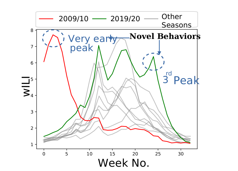
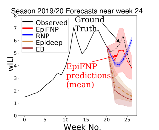
Figure 1 shows an example of a well-calibrated forecast due to EpiFNP in flu forecasting. CDC is interested in forecasting weighted Influenza-like-illness (wILI) counts, where ILI is defined as “fever and a cough and/or a sore throat without a known cause other than flu. Figure 1 (a) shows the historical ILI data with abnormal seasons highlighted; Figure (b) shows how our method EpiFNP, in contrast to others, is able to react well to a particularly novel event (in this case, introduction of a symptomatically similar COVID-19 disease), giving both accurate and well-calibrated forecasts.

Our main contributions are:
$\bullet$ Probabilistic Deep Generative Model: We design a neural Gaussian processes model for epidemic forecasting, which automatically learns stochastic correlations between query sequences and historical data sequences for non-parametic uncertainty quantification.
$\bullet$ Calibration and Explainability: EpiFNP models the output forecast distribution based on similarity between the current season and the historical seasons in a latent space. We introduce additional latent variables to capture global information of historical seasons and local views of sequences, and show that this leads to better-calibrated forecasts. Further, the relations learned between the current season and similar patterns from previous seasons enable explaining the predictions of EpiFNP.
$\bullet$ Empirical analysis of accurate well-calibrated forecasting: We perform rigorous benchmarking on flu forecasting and show that EpiFNP significantly outperforms strong baselines, providing up to 2.5x more accurate and 2.4x better calibrated forecasts. We also use outlier seasons to show the uncertainty in EpiFNP makes it adapt well to unseen patterns compared with baselines.

2 Problem and Background

We focus on epidemic disease forecasting in this paper. Our goal is to predict the disease incidence few week into the future given the disease surveillance dataset containing incidence from the past seasons as well as for the past weeks of the current season. This is formulated as a supervised time-series forecasting problem as follows.

Epidemic Forecasting task: Let the incidence for season $i$ at week $t$ be $x_{i}^{(t)}$. During the current season $N+1$ and current week $t$, we first have the snippet of time-series values upto week $t$ denoted by $\mathbf{x}_{N+1}^{(1\dots t)}=\{x_{N+1}^{(1)},\dots,x_{N+1}^{(t)}\}$. We are also provided with data from past historical seasons $1$ to $N$ denoted by $H=\{\mathbf{x}_{i}^{(1\dots T)}\}_{i=1}^{N}$ where $T$ is number of weeks per season. In real-time forecasting, intuitively our goal is to use all the currently available data, and predict the next few future values (usually till 4 weeks in future). That is to predict the value $y_{N+1}^{(t)}=x_{N+1}^{(t+k)}$, $k$ week in future where $k\in\{1,2,3,4\}$ given $\mathbf{x}_{N+1}^{(1\dots t)}$ and $H$. Formally, our task is: given (a) the dataset of historical incidence sequences $H$ and (b) snippet of incidence for current season $N+1$ till week $t$, $x_{N+1}^{(1...t)}$, estimate an accurate prediction for $y_{N+1}^{(t)}$ and a well-calibrated probability distribution $\hat{p}(y_{N+1}^{(t)}|\mathbf{x}_{N+1}^{(1...t)},H)$. There are several ways to evaluate such forecasts [40], which we elaborate later in our experiments.

3 Our Methodology

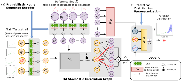
Overview: EpiFNP aims to produce calibrated forecasting probabilistic distribution. One popular choice is to use BNNs [3, 9] which impose probability distributions for weight parameters. However, as Deep Sequential Models (DSMs) have an enormous number of uninterpretable parameters, it is impractical to specify proper prior distributions in the parameter space. Existing works usually adopt simple distributions [3, 35], e.g., independent Gaussian distribution, which could severely under-estimate the true uncertainty [21]. To solve this issue, we propose EpiFNP, which combines (1) the power of DSMs in representation learning and capturing temporal correlations; and (2) the power of Gaussian processes (GPs) in non-parametric uncertainty estimation directly in the functional space similar to [26], instead of learning probability distributions for model parameters.

During training phase of our supervised learning task, EpiFNP is trained to predict $x_{i}^{(t+k)}$ given $x_{i}^{(1...t)}$ as input for $i\leq N$. Therefore, we define the training set $M$ as set of partial sequences and their forecast ground truths from historical data $H$, i.e, $M=\{(\mathbf{x}_{i}^{(1...t)},y_{i}^{(t)}):i\leq N,t+k\leq T,y_{i}^{(t)}=x_{i}^{(t+k)}\}$. For simplicity, let $\mathbf{X}_{M}$ be set of the partial sequences in $M$ and $\mathbf{y}_{M}$ the set of ground truth labels. Following GPs for non-parametric uncertainty quantification, EpiFNP constructs the forecasting distribution on the historical sequences. Since the number of possible sequences that can be extracted from $H$ is prohibitively large, we narrow down the set of candidates into a set of sequences that comprehensively represents $H$, called the reference set $R$. We choose the set of full sequences of $T$ incidence values for each season as reference set, i.e, $R=\{\mathbf{x}_{i}^{(1...T)}\}_{i=1}^{N_{R}}$. We refer elements of $M$ as $\{\mathbf{x}_{i}^{M},y_{i}^{M}\}_{i=1}^{N_{M}}$ and $R$ as $\{\mathbf{x}_{i}^{M}\}_{i=1}^{N_{R}}$ when we don’t need to specify the week and season. Also let $\mathbf{X}_{\mathcal{D}}=\{\mathbf{x}_{i}^{M}\}_{i=1}^{N_{M}}\cup\{\mathbf{x}_{i}^{R}\}_{i=1}^{N_{R}}$, the union of reference and training sequences.

The generative process of EpiFNP includes three key steps (also see Figure 2 and Eq. 1):

Figure 2: Pipeline of proposed EpiFNP model. (i) Three main components (a), (b) and (c) correspond to the terms in Equation 1. (ii) Variables highlighted in Red correspond to steps specific to inference of sequence $\mathbf{x}_{3}^{M}$.

1. Probabilistic neural sequence encoding (Section 4.2). The first step of the generative process is to use a DSM to encode the sequence $\mathbf{x}_{i}\in\mathbf{X}_{\mathcal{D}}$ into a variational latent embedding $\mathbf{u}_{i}\in\mathbf{U}_{\mathcal{D}}$. The representation power of DSM helps us to model complex temporal patterns within sequences, while the probabilistic encoding framework enables us to capture the uncertainty in sequence embedding.

2. Stochastic correlation graph construction (Section 4.3). The second step is to capture the correlations between reference ($\mathbf{U}_{R}$) and training ($\mathbf{U}_{M}$) data points in the latent embedding space (i.e. seasonal similarity between epidemic curves). We use a stochastic data correlation graph $\mathbf{G}$, which plays a similar role to the covariance matrix in classic GPs. It encodes the dependencies between reference and training sequences, enabling non-parametric uncertainty estimation.

3. Final predictive distribution parameterization (Section 4.4). Finally, we parameterize the predictive distribution with three stochastic latent variables: (1) The global stochastic latent variable $\mathbf{v}$, which is shared by all the sequences. This variable captures the overall information of the underlying function based on all the reference points. (2) The local stochastic latent variables $\mathbf{Z}_{M}=\{\mathbf{z}_{i}^{M}\}_{i=1}^{N_{M}}$. This term captures the data correlation uncertainty based on the stochastic data correlation graph $\mathbf{G}$. (3) The stochastic sequence embeddings $\mathbf{U}_{M}=\{\mathbf{u}^{M}_{i}\}_{i=1}^{N_{M}}$. This term captures the embedding uncertainty and provide additional information beyond the reference set.

Hence, putting it all together from the generative process, we factorize the predictive distribution of the training sequences into three corresponding parts ($\theta$ is the union of the parameters in EpiFNP):

$$\begin{split}&p(\mathbf{y}_{M}|\mathbf{X}_{M},R)=\sum_{\mathbf{G}}\int\underbrace{p_{\theta}(\mathbf{U}_{\mathcal{D}}|\mathbf{X}_{\mathcal{D}})}_{\text{(a)}}\underbrace{p(\mathbf{G}|\mathbf{U}_{\mathcal{D}})}_{\text{(b)}}\\ &\underbrace{p_{\theta}(\mathbf{Z}_{M},|\mathbf{G},\mathbf{U}_{R})p_{\theta}(\mathbf{v}|\mathbf{U}_{R})p_{\theta}(\mathbf{y}_{M}|\mathbf{U}_{M},\mathbf{Z}_{M},\mathbf{v})}_{\text{(c)}}d\mathbf{U}_{\mathcal{D}}d\mathbf{Z}_{M}d\mathbf{v}.\end{split}$$ (1)

Compared to existing recurrent neural process (RNP) [31] for sequential data (and its related predecessors [11, 17]), our EpiFNP process has stronger representation power and is more interpretable. Specifically, RNP uses a single global stochastic latent variable to capture the functional uncertainty, which is not flexible enough to represent a complicated underlying distribution. In contrast, EpiFNP constructs three stochastic latent variables to capture the uncertainty from different perspectives and can interpret the prediction based on the correlated reference sequences.

3.1 Probabilistic Neural Sequence Encoder

The probabilistic neural sequence encoder $p_{\theta}(\mathbf{U}_{D}|\mathbf{X}_{D})$ aims to model the complex temporal correlations of the sequence for accurate predictions of $y$, while capturing the uncertainty in the sequence embedding process. To this end, we design the sequence encoder as a RNN and stack a self-attention layer to capture long-term correlations. Moreover, following Variational auto-encoder (VAE) [18], we model the latent embedding $\mathbf{u}_{i}$ as a Gaussian random variable to capture embedding uncertainty.

We encode all the sequences, including reference sequences and training sequences, independently. Taking one sequence $\mathbf{x}_{i}$ as an example, we first feed $\mathbf{x}_{i}$ into a Gated Recurrent Unit (GRU) [7]:

$$\{\mathbf{h}_{i}^{(1)}\dots,\mathbf{h}_{i}^{(t)}\}=\text{GRU}(\{x_{i}^{(1)}\dots,x_{i}^{(t)}\}).$$ (2)

where $\mathbf{h}_{i}^{(t)}$ denotes the hidden state at time step $t$. To obtain the embedding of $\mathbf{x}_{i}$, the simplest way is to directly use the last step hidden state, $\mathbf{h}^{(t)}$. However, using the last step embedding is inadequate for epidemic forecasting as the estimates for ILI surveillance data are often delayed and revised multiple times before they stabilize [1]. Over-reliance over the last step hidden state would harm the predictive ability of the model. Therefore, we choose to use a self-attention layer [41] to aggregate the information of the hidden states across all the time steps:

$$\{{\alpha}_{i}^{(1)}\dots,{\alpha}_{i}^{(t)}\}=\text{Self-Atten}(\{{\mathbf{h}}_{i}^{(1)}\dots,{\mathbf{h}}_{i}^{(t)}\}),\quad\quad\bar{\mathbf{h}}_{i}=\sum_{t^{\prime}=1}^{t}\alpha_{i}^{(t^{\prime})}\mathbf{h}_{i}^{(t^{\prime})},$$ (3)

where $\bar{\mathbf{h}}_{i}$ is the summarized hidden state vector. Compared with the vanilla attention mechanism [2], self-attention is better at capturing long-term temporal correlations [41]. Though $\bar{\mathbf{h}}_{i}$ has encoded the temporal correlations, it is deterministic and cannot represent embedding uncertainty. Inspired by VAE, we parameterize each dimension of the latent embedding $\mathbf{u}_{i}$ as a Gaussian random variable:

$$p_{\theta}([\mathbf{u}_{i}]_{k}|\mathbf{x}_{i})=\mathcal{N}([g_{1}(\bar{\mathbf{h}}_{i})]_{k},\exp([g_{2}(\bar{\mathbf{h}}_{i})]_{k})),$$ (4)

where $g_{1}$ and $g_{2}$ are two multi-layer perceptrons (MLPs), $[\cdot]_{k}$ is the $k$-th dimension of the variable.

3.2 Stochastic Data Correlation Graph

The stochastic graph $\mathbf{G}$ is used to model the correlations among sequences, which is central to the non-parametric uncertainty estimation ability of EpiFNP. It is realized by constructing a bipartite graph from the reference set $R$ to the training set $M$ based on the similarity between their sequence embeddings. With this graph, we aim to model the dynamic similarity among epidemic curves as in [1] but in a stochastic manner, which allows us to further quantify the uncertainty coming from our latent representations of the sequences. Note that the similarity with reference sequence embeddings dynamically changes across the current season since different periods of the season may be similar to different sets of reference sequences (as we illustrate in Section 4.4).

We first construct a complete weighted bipartite graph $\mathbf{G}_{c}$ from $R$ to $M$, where the nodes are the sequences. The weight of each edge is calculated as similarity between two sequences in the embedding space using the radial basis function kernel $\kappa(\mathbf{u}^{R}_{i},\mathbf{u}^{M}_{j})=\exp(-\gamma||\mathbf{u}^{R}_{i}-\mathbf{u}^{M}_{j}||^{2})$. Modeling such a similarity in the embedding space is more accurate than in the input space by leveraging the representation power of the neural sequence encoder.

Though we can directly use $\mathbf{G}_{c}$ to encode the data correlations, such a dense complete graph

Figure 3: We sample the (sparse) binary graph $\mathbf{G}$ from the complete weighted (dense) graph $\mathbf{G}_{c}$.

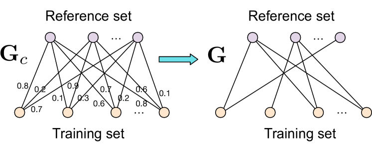
requires heavy computations and does not scale to a large dataset. Therefore, we choose to further sample from this complete graph to obtain a stochastic binary bipartite graph $\mathbf{G}$ as shown in Figure 3. This graph can be represented as a random binary adjacency matrix, where $\mathbf{G}_{i,j}=1$ means the reference sequence $\mathbf{x}_{i}^{R}$ is a parent of the training sequence $\mathbf{x}_{j}^{M}$. We then parameterize this binary adjacency matrix using Bernoulli distributions:

$$p(\mathbf{G}|\mathbf{U}_{\mathcal{D}})=\prod_{i\in R}\prod_{j\in M}\text{Bernoulli}(\mathbf{G}_{i,j}|\kappa(\mathbf{u}_{i}^{R},\mathbf{u}_{j}^{M})).$$ (5)

Intuitively, the edges in $\mathbf{G}_{c}$ with higher weights are more likely to be kept after sampling. This sampling process leads to sparse correlations for each sampled graph, which can speed up training due to sparsity.

3.3 Parameterizing Predictive Distribution

Here we introduce how to parameterize the final prediction based on the three latent variables mentioned in Section 4.1, which capture the functional uncertainty from different perspectives.

Local latent variable $\mathbf{z}_{i}^{M}$: It summarizes the information of the correlated reference points for each training point and captures the uncertainty of data correlations. We generate $\mathbf{z}_{i}^{M}$ based on the structure of the data correlation graph, and each dimension $k$ follows a Gaussian distribution:

$$\mathbf{z}_{i,k}^{M}\sim\mathcal{N}(C_{i}\sum_{j:\mathbf{G}_{j,i}=1}h_{1}(\mathbf{u}_{j}^{R})_{k},\exp(C_{i}\sum_{j:\mathbf{G}_{j,i}=1}h_{2}(\mathbf{u}_{j}^{R})_{k})),$$ (6)

where $h_{1}$ & $h_{2}$ are two MLPs and $C_{i}=\sum_{j}\mathbf{G}_{i,j}$ is for normalization. As we can see from Equation 6, if the sequence has lower probability to be connected with the reference sequences, $\mathbf{z}_{i}^{M}$ becomes a standard Gaussian distribution which is an uninformative prior. This property imposes a similar inductive bias as in the GPs with RBF kernel.

Global latent variable $\mathbf{v}$. It encodes the information in all the reference points, computed as:

$$\beta_{1},\dots,\beta_{N_{R}}=\text{Self-Atten}(\mathbf{u}^{R}_{1},\dots,\mathbf{u}^{R}_{N_{R}}),\quad\quad\quad\mathbf{v}=\sum_{i=1}^{N_{R}}\beta_{i}\mathbf{u}_{i}^{R}.$$ (7)

In contrast with the local variable $\mathbf{z}_{i}^{M}$, the global latent variable $\mathbf{v}_{i}$ summarizes the overall information of the underlying function. It is shared by all the training sequences which allows us to capture the functional uncertainty from a global level.

Sequence embedding $\mathbf{u}_{i}^{M}$: The above two latent variables are both constructed from the embeddings of the reference sequences, which may lose novel information present in the training sequences. Therefore, we add a direct path from the latent embedding $\mathbf{u}^{M}_{i}$ of the training sequence to the final prediction to enable the neural network to extrapolate beyond the distribution of the reference sequences. This is useful in novel/unprecedented patterns where the input sequence can not rely only on reference sequences from historical data for prediction.

We concatenate the three variables together into a single vector $\mathbf{e}_{i}$ and obtain the final predictive distribution (where $d_{1}$ and $d_{2}$ are MLPs):

$$\mathbf{e}_{i}=\text{concat}(\mathbf{z}_{i},\mathbf{v}_{i},\mathbf{u}_{i}),\quad\quad\quad p(y_{i}|\mathbf{z}_{i}^{M},\mathbf{v},\mathbf{u}_{i}^{M})=\mathcal{N}(d_{1}(\mathbf{e}_{i}),\exp(d_{2}(\mathbf{e}_{i}))).$$ (8)

3.4 Learning the distribution

We now introduce how to learn the model parameters efficiently during training and forecast for a new unseen sequence at test time. Directly maximizing the data likelihood is intractable due to the summation and integral in Equation 1. Therefore, we choose to use the amortized variational inference and approximate the true posterior $p(\mathbf{U}_{\mathcal{D}},\mathbf{G},\mathbf{Z}_{M},\mathbf{v}|R,M)$ with $q_{\phi}(\mathbf{U}_{\mathcal{D}},\mathbf{G},\mathbf{Z}_{M},\mathbf{v}|R,M)$, similar to [26], as

$$q_{\phi}(\mathbf{U}_{\mathcal{D}},\mathbf{G},\mathbf{Z}_{M},\mathbf{v}|R,M)=p_{\theta}(\mathbf{U}_{\mathcal{D}}|\mathbf{X}_{\mathcal{D}})p(\mathbf{G}|\mathbf{U}_{\mathcal{D}})p(\mathbf{v}|\mathbf{U}_{R})q_{\phi}(\mathbf{Z}_{M}|M).$$ (9)

We design $q_{\phi}$ as a single layer of neural network parameterized by $\phi$, which outputs mean and variance of the Gaussian distribution $q_{\phi}(\mathbf{Z}_{M}|\mathbf{X}_{M})$.

We then use a gradient-based method, such as Adam [18], to maximize the evidence lower bound (ELBO) of the log likelihood. After canceling redundant terms, the ELBO can be written as:

$$\begin{split}\mathcal{L}=-\mathrm{E}_{\mathbf{Z}_{M},\mathbf{G},\mathbf{U}_{\mathcal{D}},\mathbf{v}\sim q_{\phi}(\mathbf{Z}_{M}|\mathbf{X}_{M})p_{\theta}(\mathbf{G},\mathbf{U}_{\mathcal{D}},\mathbf{v}|\mathcal{D})}&[\log P(\mathbf{y}_{M}|\mathbf{Z}_{M},\mathbf{U}_{M},\mathbf{v})\\ +\log P(\mathbf{Z}_{M}|\mathbf{G},\mathbf{U}_{R})-q_{\phi}(\mathbf{Z}_{M}|\mathbf{X}_{M})].\end{split}$$ (10)

We use the reparameterization trick to make the sampling procedure from the Gaussian distribution differentiable. Moreover, as sampling from the Bernoulli distribution in Equation 7 leads to discrete correlated data points, we make use of the Gumbel softmax trick [15] to make the model differentiable.

At test time, with the optimal parameter $\theta_{\rm opt}$, we base the predictive distribution of a new unseen partial sequence $\mathbf{x}^{*}$ on the reference set as:

$$\begin{split}p(y^{*}|R,\mathbf{x}^{*})=&p_{\theta_{\rm opt}}(\mathbf{U}_{R},\mathbf{u}^{*}|\mathbf{X}_{M},\mathbf{x}^{*})p(\mathbf{a}^{*}|\mathbf{U}_{R},\mathbf{u}^{*})\\ &p_{\theta_{\rm opt}}(\mathbf{z}^{*}|\mathbf{a}^{*},\mathbf{U}_{R},\mathbf{u}^{*})p_{\theta_{\rm opt}}(y^{*}|\mathbf{u}^{*},\mathbf{z}^{*},\mathbf{v})d\mathbf{U}_{R}d\mathbf{z}^{*}d\mathbf{v},\end{split}$$ (11)

where $\mathbf{a}^{*}$ is the binary vector that denotes which reference sequences are the parents of the new sequence. $\mathbf{u}^{*}$ and $\mathbf{z}^{*}$ are latent embedding and local latent variable for the new sequence, respectively.

4 Experiments

All experiments were done on an Intel i5 4.8 GHz CPU with Nvidia GTX 1650 GPU. The model typically takes around 20 minutes to train. The code is implemented using Pytorch and will be released for research purposes. Supplementary contains additional details and results (e.g. hyperparameters, results on additional metrics (MAPE), additional case and ablation studies).

Dataset: In our experiments, we focus on flu forecasting. The CDC uses the ILINet surveillance system to gather flu information from public health labs and clinical institutions across the US. It releases weekly estimates of weighted influenza-like illness (wILI): out-patients with flu-like symptoms aggregated for US national and 10 different regions (called HHS regions). Each flu season begins at week 21 and ends on week 20 of the next year e.g. Season 2003/04 begins on week 21 of 2003 and ends on week 20 of 2004. Following the guidelines of CDC flu challenge [1, 34], we predict from week 40 till the end of season next year. We evaluate our approach using wILI data of 17 seasons from 2003/04 to 2019/20 .

Goals: Our experiments were designed evaluate the following. Q1: Accuracy and calibration of EpiFNP’s forecasts. Q2: Importance of different components of EpiFNP. Q3: Utility of uncertainty estimates for other related tasks?. Q4: Adaptability of EpiFNP to novel behaviors during real-time forecasting. Q5: Explainability of predictions.

Evaluation metrics: Let $x_{N+1}^{1...t}$ be a given partial wILI test sequence with observed ground truth $y_{N+1}^{(t)}$ i.e., for a $k$-week-ahead task $y_{N+1}^{(t)}$ is just $x_{N+1}^{(t+k)}$. For a model/method $M$ let $\hat{p}_{N+1,M}^{(t)}(Y)$ be the output distribution of the forecast with mean $\hat{y}_{N+1,M}^{(1...t)}$. To measure the predictive accuracy, we use Root Mean Sq. Error (RMSE), Mean Abs. Per. Error (MAPE) and Log Score (LS) which are commonly used in CDC challenges [1, 34]). To evaluate the calibration of the predictive distribution we introduce a new metric called Calibration Score (CS). For a model $M$ we define a function $k_{M}:[0,1]\rightarrow[0,1]$ as follows. For each value of confidence $c\in[0,1]$, let $k_{M}(c)$ denote the fraction of observed ground truth that lies inside the $c$ confidence interval of predicted output distributions of $M$. For a perfectly calibrated model $M^{*}$ we would expect $k_{M^{*}}(c)=c$. CS measures the deviation of $k_{M}$ from $k_{M^{*}}$. Formally, we define CS as:

$$CS(M)=\int_{0}^{1}|k_{M}(c)-c|dc\approx 0.01\sum_{c\in\{0,0.01,\dots,1\}}|k_{M}(c)-c|.$$ (12)

For all metrics, lower is better. We also define the Calibration Plot (CP) as the profile of $k_{M}(c)$ vs $c$ for all $c\in[0,1]$.

Baselines: We compare EpiFNP with standard and state-of-art models used for flu forecasting before, as well as methods typically used for learning calibrated uncertainty quantification.
Flu forecasting related: $\bullet$ SARIMA: Seasonal Autoregressive Integrated Moving-Average is a auto-regressive time series model used as baseline for forecasting tasks [1, 44]. $\bullet$ Gated Recurrent Unit (GRU): A popular deep learning sequence encoder, used before as a baseline for this problem [1]. $\bullet$ Empirical Bayes (EB): Utilizes a bayes framework and has won few epidemic forecasting competitions in past [4]. $\bullet$ Delta Density (DD): A probabilistic modelling approach that learns distribution of change in successive wILI values given changes from past weeks [5]. $\bullet$ Epideep (ED) [1]: Recent state-of-the-art NN flu prediction model based on learning similarity between seasons. $\bullet$ Gaussian Process (GP) [44]: Recently proposed statistical flu prediction model using GPs. Note that ED, SARIMA and GRU can only output point estimates and we use the ensemble approach to obtain their uncertainty estimates following [34, 6].
General ML Uncertainty related: $\bullet$ Monte Carlo Dropout (MCDP) [10]: MCDP applies dropout at testing time for multiple times to measure the uncertainty. We use MCDP on a GRU as a baseline. $\bullet$ Bayesian neural network (BNN) [3]: BNN imposes and learns from probability distributions over model parameters. We used LSTM as the architecture for BNN $\bullet$ Recurrent Neural Process (RNP) [31]: This method builds on Neural Process framework to learn from sequential data.

Note: We need to train EpiFNP only once at start of a season using data from all past seasons unlike some baselines (ED, EB, GP, SARIMA, DD) which require retraining each week.

4.1 Q1 & Q2: Forecast Accuracy, Calibration and Model Ablation

Table 1: Average US National Performance: $k$ week ahead forecasting for seasons 2014/15-2019/20.

	RMSE			MAPE			LS			CS
Model	k=2	k=3	k=4	k=2	k=3	k=4	k=2	k=3	k=4	k=2	k=3	k=4
ED	0.73	1.13	1.81	0.14	0.23	0.33	4.26	6.37	8.75	0.24	0.15	0.42
GRU	1.72	1.87	2.12	0.28	0.31	0.356	7.98	8.21	8.95	0.16	0.2	0.22
MCDP	2.24	2.41	2.61	0.46	0.51	0.6	9.62	10	10	0.24	0.32	0.34
GP	1.28	1.36	1.45	0.21	0.22	0.26	2.02	2.12	2.27	0.24	0.25	0.28
BNN	1.89	2.05	2.43	0.34	0.46	0.51	6.92	7.56	8.03	0.18	0.22	0.25
SARIMA	1.43	1.81	2.12	0.28	0.35	0.42	3.11	3.4	3.81	0.43	0.38	0.34
RNP	0.61	0.98	1.18	0.13	0.22	0.29	3.34	3.61	3.89	0.43	0.46	0.45
EB	1.21	1.23	1.25	0.57	0.58	0.58	6.92	7	7.12	0.07	0.082	0.085
DD	0.6	0.79	0.94	0.35	0.41	0.45	3.56	3.87	4.02	0.12	0.12	0.13
EpiFNP	0.48	0.79	0.78	0.089	0.128	0.123	0.56	0.84	0.89	0.068	0.081	0.035

Prediction Accuracy: We first compare the accuracy of EpiFNP against all baselines for real-time forecasting in Table 1. EpiFNP significantly outperforms all other baselines for RMSE, MAPE, LS (which measure forecast accuracy). We notice around 13% and 42% improvement over the second best baseline in RMSE and MAPE respectively. Impressively LS of EpiFNP is 2.5 to 3.5 times less than closest baseline. This is because the intervals $y_{i}^{(t)}\pm 0.5$ of ground truth consistently fall inside high probability regions of our forecast distribution due to better accuracy (of mean) in general. Even during weeks of uncertainty (like around the peaks) most baselines badly calibrated forecasts don’t sufficiently cover the interval, EpiFNP’s distribution are wide enough to capture this interval thanks to its superior representation power. We also observed similar results for the 10 HHS regions as well where EpiFNP outperforms the baselines where we show 16% and 7% improvements in RMSE ans LS respectively showing EpiFNP’s proficiency over large variety different regions and seasons.

Figure 4: Forecasts and 95% confidence bounds on 2017/18 season.

Figure 5: CPs for EpiFNP and next 3 accurate baselines, k=4

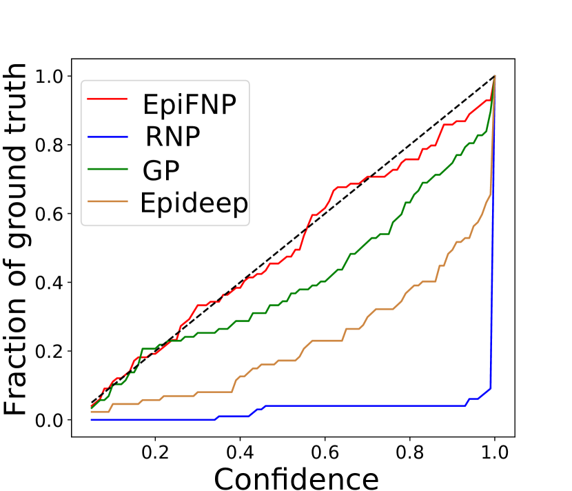
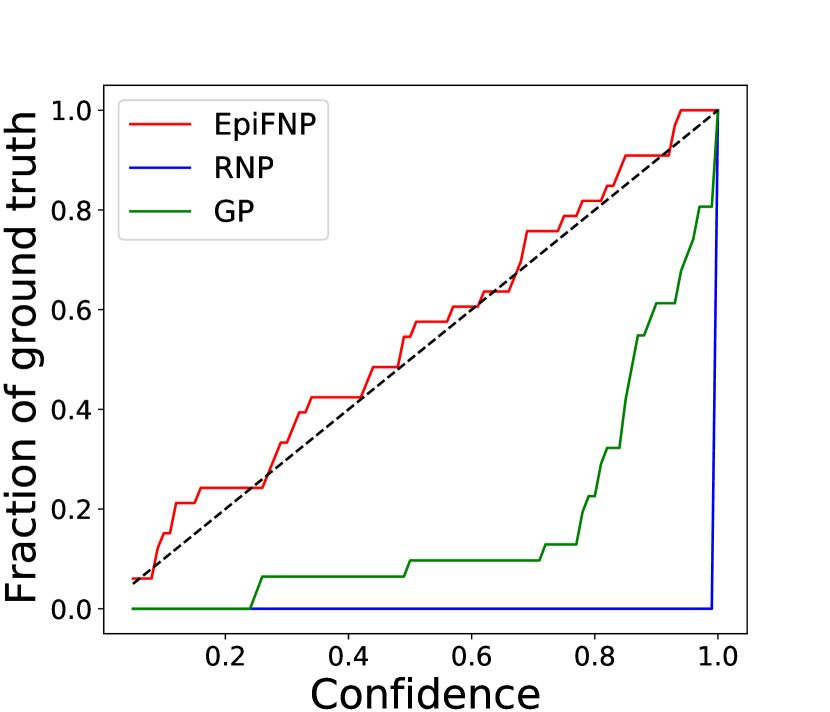
Calibration Quality: We measure how well-calibrated EpiFNP’s uncertainty bounds (Figure 5) are via CS. EpiFNP was again the clear winner both for national forecasts (Table 1) and regional forecasts. Calibration Plots (CPs) (Figure 5) show EpiFNP is much closer to the diagonal line (ideal calibration) compared to even the most competitive baselines. We also observed that applying post-hoc calibration methods [23, 39] doesn’t effect the significance of EpiFNP’s calibration performance (Appendix Table 4). EpiFNP is clearly significantly superior to all other baselines in predicting both a better calibrated and more accurate forecast distribution.

Ablation studies: We found all three of our EpiFNP components important for performance, with the data correlation graph the most relevant in determining uncertainty bounds. Refer to supplementary for complete results and further discussion.

4.2 Q3: Effective uncertainty estimates: Autoregressive inference

Motivation: We further show the usefulness and quality of our uncertainty estimates by leveraging the so-called ’auto-regressive’ inference (ARI) task. It is common to perform such forecasting in real-time epidemiological settings, especially as accuracy and training data typically drops with increasing $k$ week-ahead in future [37]. In this task, the model uses its own output for $k=1$ forecast as input (multiple samples) to predict $k=2$ forecasts and so on to derive $k$-week ahead prediction. Hence an inaccurate and badly calibrated initial model’s forecasts propagate their errors to subsequent predictions as well.

Table 2: Evaluation scores for ARI task.

	RMSE			LS			CS
Model	k=2	k=3	k=4	k=2	k=3	k=4	k=2	k=3	k=4
ED	2.21	3.13	3.82	6.03	8.84	10	0.42	0.45	0.48
MCDP	3.62	4.03	4.39	10	10	10	0.47	0.46	0.49
BNN	3.41	4.23	4.78	10	10	10	0.39	0.41	0.42
GP	1.24	1.31	1.38	4.62	5.17	5.51	0.37	0.36	0.37
EpiFNP	0.6	0.85	0.99	0.64	0.96	1.14	0.063	0.074	0.048

We perform forecasting for $k=2,3,4$ week ahead as described above using the $k=1$ trained model. The pseudocode for Autoregressive inference is given in the Appendix.

Results: See Table 2. Only baselines not trained autoregressively by default (as EpiFNP already outperforms them (Q1)) are considered. EpiFNP outperforms all and is comparable even to the non AR trained original EpiFNP scores (Table 1) whereas we observed a significant deterioration in scores for other baselines, as anticipated.

4.3 Q4: Reacting to abnormal/novel patterns

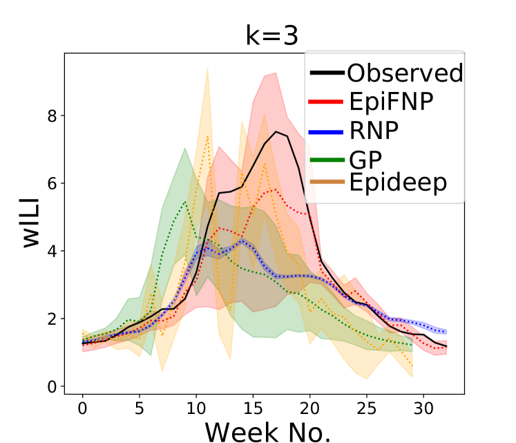
Motivation: A major challenge in real-time epidemiology [36] is the presence of novel patterns e.g. consider the impact of the COVID-19 pandemic on the 2019/20 wILI values (see Figure 1(a)). In such cases, a trustworthy real-time forecasting model to anticipate, quantify and adapt is needed to such abnormal situations. We studied our performance for the 2009/10 and 2019/20 seasons, which are well known abnormal seasons (due to the H1N1 strain and the COVID-19 pandemic respectively). While we discuss results for $k=3$ week ahead forecasting of 2019/20 season, the results for 2009/10 season and for $k=1,2,4$ lead to similar conclusions.

(a) 2019/20 predictions

(b) 2019/20 CP

Figure 6: EpiFNP outperforms top 2 baselines during abnormal COVID-19 season 2019/20.

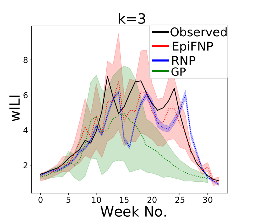
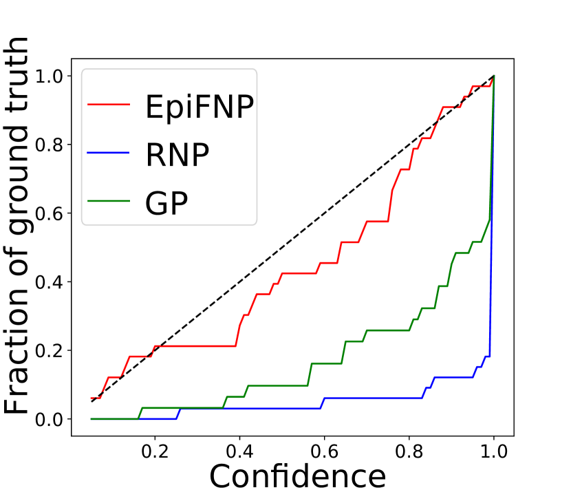
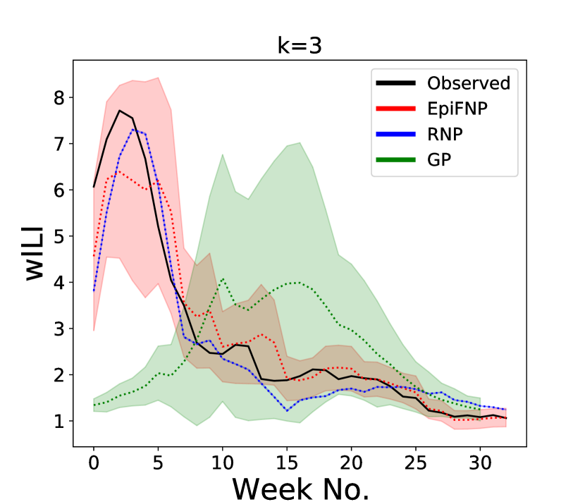
Results: In short, EpiFNP reacts reliably and adapts to novel scenarios. EpiFNP outperforms other baselines in all metrics. We observed 18% and 31% reduction in RMSE and MAPE respectively compared to best baseline (RNP) and 3.7 times lower LS compared to best baseline (GP). Figure 6(a) shows the prediction and uncertainty bounds of EpiFNP and top 2 baselines. GP and most other baselines (except RNP) fail to capture the unprecedented third peak around week 24. Calibration Plot in Figure 6(b) shows that EpiFNP is better calibrated.

4.4 Q5: Explainable Predictions

Motivation: Lack of explainability is a major challenge in many ML models, which becomes even more acute in critical domains like public health. Since the Stochastic data correlation graph (SDCG) of EpiFNP (recall Section 3.2) explicitly learns to relate each test sequence with relevant historical seasons’ sequences, we can leverage this to provide useful explanations for predictions and model uncertainty. Knowing which past seasons are similar is very helpful for epidemiological understanding of the prevalent strain behavior [1]. We sample SDCGs multiple times and compute average edge probability for every edge between each given historical season and test sequences during real-time forecasting for all weeks. We perform this for $k=3$ weeks ahead forecasting on season 2015/16 but the observations hold for other seasons and $k=1,2,4$ too.

Figure 7: 2015/16 snippet & most similar seasons chosen by EpiFNP.

Figure 8: Average edge probabilities for week 21 of 2015/16 season.

Obs 1: EpiFNP automatically chooses most similar historical seasons relevant at time of prediction.
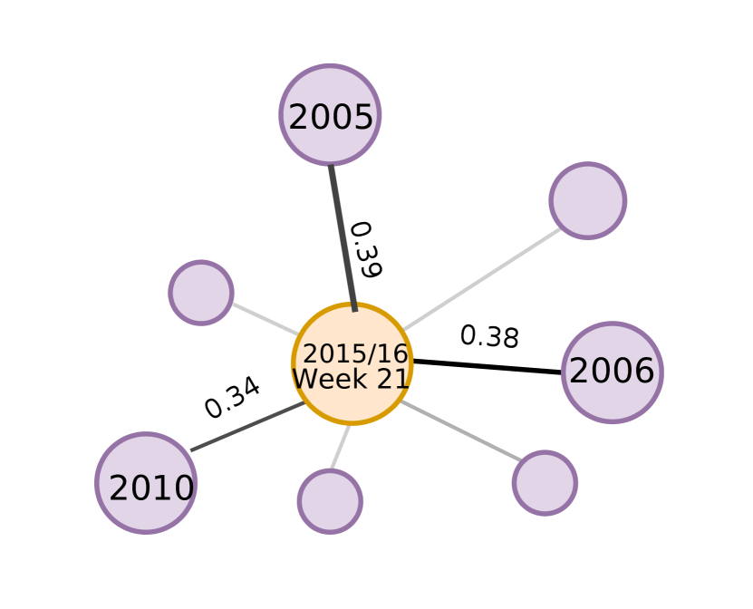
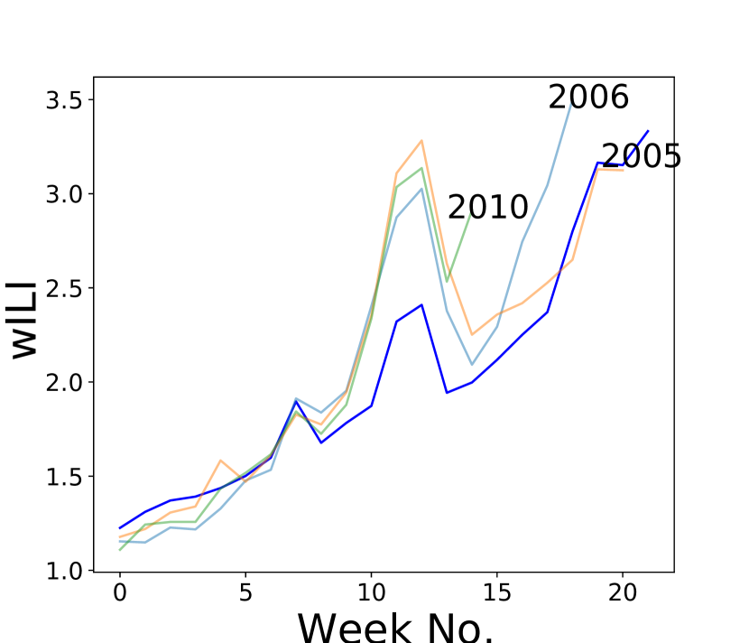
We leverage the edge probabilities from the SDCG to examine the seasons that are more likely sampled at at each week. We observed that the seasons with higher probabilities showed similar patterns to that of the current test sequence. Consider week 21 of season 2015/16 during 3 weeks ahead forecasting. The most likely sampled seasons are 2005, 2006 and 2010 (Figure 8). Figure 8 shows these seasons and 2015/16 snippet; clearly they have very similar wILI patterns.

Obs 2: EpiFNP explains uncertainty bounds of predictions via distribution probabilities in the SDCG.

Figure 9: Higher uncertainty around peaks

Figure 10: SDCG Avg. edge probabilities

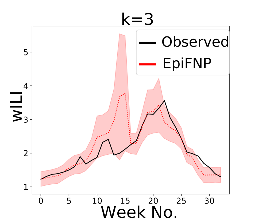
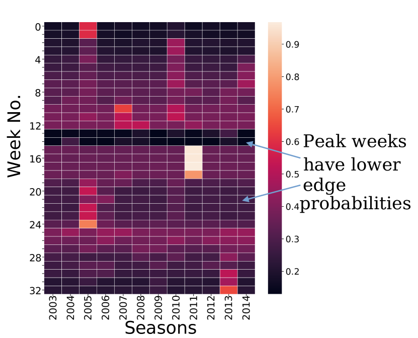
As seen in Section 4.3, EpiFNP reacts reliably to abnormal situations and changing trends (e.g. around peaks) by producing larger uncertainty bounds around those events. For example, in Figure 10, uncertainty estimates around peak weeks 12 and 22 are higher than for rest of the weeks. To examine the source of changing uncertainty bounds of prediction, we look at average edge probabilities generated in SDCG (Figure 10) and find that around the peak weeks the edge probabilities are lower than in surrounding weeks. This promotes larger variety of small subsets of the reference set to be sampled during inference that increases the variance of local latent variable $\mathbf{z}_{i}^{M}$ thereby increasing the variance of the output forecast distribution.

5 Conclusion

We introduced EpiFNP, a novel deep probabilistic sequence modeling method which generates well calibrated, explainable and accurate predictions. We demonstrated its superior performance in the problem of real-time influenza forecasting by significantly outperforming other non-trivial baselines (more than 2.5x in accuracy and upto 2.4x in calibration). Importantly, it was the only one capable of reliably handling unprecedented scenarios e.g. H1N1 and COVID19 seasons. We also showcased its explainability as it automatically retrieves the most relevant historical sequences matching its current week’s predictions using the SDCG. All these highlight the usefulness of EpiFNP for the complex challenge of trustworthy epidemiological forecasting, which directly impacts public health policies and planning. However EpiFNP can be affected by any systematic biases in data collection (for example, some regions might have poorer surveillance and reporting capabilities). There is limited potential for misuse of our algorithms and/or data sources though the dataset is public/anonymized without any sensitive patient information.

We believe our work opens up many interesting future questions. Our setup can be easily extended to handle other diseases and our core technique can be adapted for other general sequence modeling problems. Further, we can extend EpiFNP to also use heterogeneous data from multiple sources. We can also explore incorporating domain knowledge of prior dependencies between different sources/features (e.g. geographically close regions are more likely to have similar disease trends).

Acknowledgments: We thank the anonymous reviewers for their useful comments. This work was supported in part by the NSF (Expeditions CCF-1918770, CAREER IIS-2028586, RAPID IIS-2027862, Medium IIS-1955883, Medium IIS-2106961, CCF-2115126, Small III-2008334), CDC MInD program, ORNL, ONR MURI N00014-17-1-2656, faculty research awards from Facebook, Google and Amazon and funds/computing resources from Georgia Tech.

Appendix for When in Doubt: Neural Non-Parametric Uncertainty Quantification for Epidemic Forecasting

Code for EpiFNP and wILI dataset is publicly available .

Appendix A Additional Related work

Statistical models for Epidemic Forecasting In the recent years, statistical models have been the most successful in several forecasting targets, as noted in multiyear assessments  [34]. In influenza forecasting, various recent statistical approaches have been proposed. On one hand, we have models designed to model the details on the underlying generative distribution of the data. Among these, [4] proposed a semiparametric Empirical Bayes framework that constructs a prior of the current season’s epidemic curve from the past seasons and outputs a distribution over epidemic curves. [5] opts for a non-parametric approach based on kernel density estimation to model the probability distribution of the change between consecutive predictions. Closely related, Gaussian processes have been recently explored for influenza forecasting [44]. Other popular methods rely on ensembles of mechanistic and statistical methods  [32].

More recently, the deep learning community has take interest in forecasting influenza [1, 42] and COVID-19 [37]. Indeed, deep learning enables to address novel situations where traditional influenza models fail such as adapting a historical influenza model to pandemic [36]. Deep learning is also suitable because it provides the capability of ingesting data from multiple sources, which better informs the model of what is happening on the ground. However, for most of this body of work uncertainty quantification is either non existent or has been explored with simple techniques that lack of proper knowledge representation. Our work aims to close this gap in the literature.

Uncertainty Quantification for Deep Learning Recent works have shown that deep neural networks are over-confident in their predictions [12, 20]. Existing approaches for uncertainty quantification can be categorized into three lines. The first line is based on Bayesian Neural Networks (BNNs) [28, 3, 27]. They are realized by first imposing prior distributions over neural network parameters, then infer parameter posteriors and further integrate over them to make predictions. However, as exact inference of parameter posteriors is often intractable, approximation methods have also been proposed, including variational inference [3, 27], Monte Carlo dropout [10] and stochastic gradient Markov chain Monte Carlo (SG-MCMC) [25, 43]. Such BNN approximations tend to underestimate the uncertainty [21]. Moreover, specifying parameter priors for BNNs is challenging because the parameters of DNNs are huge in size and uninterpretable [21, 26].

The second line tries to combine the stochastic processes and DNNs. Neural Process (NP) [11] defines a distribution over a global latent variable to capture the functional uncertainty, while Functional neural process (FNP) [26] use a dependency graph to encode the data correlation uncertainty. However, they are both for the static data. Recently, recurrent neural process (RNP) [31, 17] has been proposed to incorporate RNNs into the NP to capture the ordering sequential information.

The third line is based on model ensembling [24] which trains multiple DNNs with different initializations and use their predictions for uncertainty quantification. However, training multiple DNNs require extensive computing resources.

Appendix B Model Hyperparameters

We describe all the hyperparameters used for the EpiFNP model including the model architecture. In general, we used the hyperparameters as done in [26] with changes made to accommodate the sequential modules and global embedding for our use case.

B.1 Architecture

B.1.1 Probabilistic Neural Sequence Encoder

The GRU for the encoder model has single hidden layer of 50 units and outputs 50 dimensional vectors. The Attention layer was similar to that used in transformers. We used a single attention head and retained the same number of dimensions, 50, when generating the key and value embeddings. to generate $\mathbf{u}_{i}$, we derived the mean and log variance using a stack of 3 linear layers for $g_{1}$ and $g_{2}$ with ReLU in between the hidden layers. All hidden layers have 50 units.

Note that for sampling from multivariate gaussian distribution, we always assumed the covariance matrix to be a diagonal matrix and only derived log variance for each dimension.

B.1.2 Parameterizing Predictive Distribution

The $h_{1}$ and $h_{2}$ functions used to derive $\mathbf{z}_{i}^{M}$ were single linear layers with no activation function. The Attention layer used to derive $\mathbf{v}$ was similar to that used in encoder: 1 attention head with 50 dimension units for key and value transforms. $d_{1}$ and $d_{2}$ are two modules of feed forward layers with a ReLU function between them with first layer having 50 units and the second having 2 to output mean and log variance of forecast output.

B.2 Other Hyperparameters

Learning rate used was $1e-4$. We also used early stopping to prevent overfitting and randomly sampled 5% of training points as validation set to determine when we reached the point of overfitting. EpiFNP usually 2000-3000 epoch to complete training. We found that our model was very robust to small changes in architecture and learning rate and we mostly optimized for faster rate of convergence during training.

Appendix C Details on Evaluation metrics

Let $x_{N+1}^{1...t}$ be a given partial wILI test sequence with observed ground truth $y_{N+1}^{(t)}$ i.e., for a $k$-week-ahead task $y_{N+1}^{(t)}$ is just $x_{N+1}^{(t+k)}$. For a model/method $M$ let $\hat{p}_{N+1,M}^{(t)}(Y)$ be the output distribution of the forecast with mean $\hat{y}_{N+1,M}^{(1...t)}$. Then we define the evaluation metrics as follows. We evaluate all the methods based on metrics for measuring prediction accuracy (RMSE, MAPE and LS are commonly used in CDC challenges [1, 34]) as well as targeted ones (CS) measuring the quality of prediction calibration of uncertainty. For all metrics, lower is better. EpiFNP is carefully designed to generate both accurate and well calibrated forecasts, unlike past work which focuses typically on accuracy only.

$\bullet$ $\mathbf{Root~{}Mean~{}Sq.~{}Error~{}RMSE}(M)=\sqrt{\frac{1}{T}\sum_{t=1}^{T}(y_{N+1}^{(t)}-\hat{y}_{N+1,M}^{(t)})^{2}}$

$\bullet$ $\mathbf{Mean~{}Abs.~{}Per.~{}Error~{}MAPE}(M)=\frac{1}{T}\sum_{t=1}^{T}\frac{|y_{N+1}^{(t)}-\hat{y}_{N+1,M}^{(t)}|}{|y_{N+1}^{(t)}|}$

$\bullet$ Log Score (LS): This score used by the CDC caters to the stochastic aspect of forecast prediction [34].

$$LS(M)=\sum_{i=1}^{T}\frac{1}{T}\int_{y_{i}^{(t)}-0.5}^{y_{i}^{(t)}+0.5}-\log(\hat{p}_{N+1,M}^{(t)}(y))dy$$ (13)

The integral is approximated by samples from $\hat{p}_{N+1,M}^{(t)}(Y)$ and calculating the fraction of samples that fall in the correct interval.

$\bullet$ Calibration Score (CS): In order to evaluate the calibration of output distribution we introduce a new metric called Calibration Score, which is inspired by reliability diagrams [29] used for binary events. The idea behind the calibration score is that a well calibrated model provides meaningful confidence intervals. For a model $M$ we define a function $k_{M}:[0,1]\rightarrow[0,1]$ as follows. For each value of confidence $c\in[0,1]$, let $k_{M}(c)$ denote the fraction of observed ground truth that lies inside the $c$ confidence interval of predicted output distributions of $M$. For a perfectly calibrated model $M^{*}$ we would expect $k_{M^{*}}(c)=c$. CS measures the deviation of $k_{M}$ from $k_{M^{*}}$. Formally, we define CS as:

$$CS(M)=\int_{0}^{1}|k_{M}(c)-c|dc\approx 0.01\sum_{c\in\{0,0.01,\dots,1\}}|k_{M}(c)-c|$$ (14)

(since integrating over all values of $c$ is intractable in general).

We also define the Calibration Plot (CP) as the profile of $k_{M}(c)$ vs $c$ for all $c\in[0,1]$.

Appendix D Detailed forecast results

D.1 Regional forecasts

We also evaluate our model and baselines on wILI dataset specific to different regions in USA. The wILI data for 10 HHS regions are available separately and each of them have different characteristics in their wILI trends which are affected by local climate, population density and other factors. Therefore we train our models on each of the HHS regions seperately and average the scores to produce the results in table 3. EpiFNP outperforms baselines in most baselines. We observed that for 8 of the 10 regions EpiFNP outperforms all models in all the evaluation metrics across 2 to 4 week ahead forecast tasks. Even for the remaining 2 regions EpiFNP shows superior scores in majority of the metrics.

Table 3: Average Evaluation scores of EpiFNP and baselines across all HHS regions. The scores are averaged over seasons 2014-15 to 2019-20 for all 10 HHS regions.

	RMSE			MAPE			LS			CS
Model	2	3	4	2	3	4	2	3	4	2	3	4
ED	0.86	1.2	1.81	0.23	0.25	0.36	2.89	2.69	3.32	0.17	0.32	0.33
GRU	1.95	2.05	2.76	0.39	0.41	0.43	4.41	4.52	4.86	0.37	0.38	0.41
MCDP	3.01	3.36	3.41	0.58	0.548	0.68	10	10	10	0.38	0.39	0.47
GP	0.64	0.83	0.95	0.19	0.22	0.25	0.92	1.44	1.63	0.13	0.16	0.15
BNN	2.25	2.87	3.02	0.26	0.29	0.35	8.31	9.89	10	0.38	0.42	0.46
SARIMA	1.81	2.33	2.8	0.36	0.47	0.58	3.3	3.87	4.37	0.39	0.37	0.37
RNP	0.87	0.88	1.17	0.19	0.23	0.29	9.27	9.58	9.78	0.46	0.46	0.47
EB	1.51	1.53	1.56	0.67	0.67	0.68	7.15	7.23	7.29	0.13	0.13	0.13
DD	0.84	1.05	1.22	0.44	0.49	0.55	3.51	3.77	3.91	0.11	0.11	0.12
EpiFNP	0.55	0.7	0.89	0.17	0.19	0.26	1.41	1.54	1.81	0.15	0.11	0.13

D.2 Post-hoc calibration methods

We also evaluated effect of post-hoc methods [23, 39] on calibration of prediction distributions of top baselines and EpiFNP. The results are summarized in Table 4. We observe that EpiFNP doesn’t benefit much from post-hoc calibration methods due to its already well-calibrated forecasts. However, they improve the calibration scores of other baselines (sometimes at the cost of prediction accuracy). However, EpiFNP is still clearly the best performing model.

Table 4: Effect of post-hoc calibration on point estimate and calibration scores. Iso and DC are the post-hoc methods introduced in [23] and [39] respectively.

		RMSE			MAPE			LS			CS
Model	Post-Hoc	k=2	k=3	k=4	k=2	k=3	k=4	k=2	k=3	k=4	k=2	k=3	k=4
EpiFNP	None	0.48	0.79	0.78	0.089	0.128	0.123	0.56	0.84	0.89	0.068	0.081	0.035
	Iso	0.49	0.81	0.79	0.09	0.124	0.119	0.56	0.86	0.9	0.08	0.09	0.07
	DC	0.44	0.74	0.77	0.088	0.114	0.117	0.55	0.75	0.86	0.07	0.08	0.035
RNP	None	0.61	0.98	1.18	0.13	0.22	0.29	3.34	3.61	3.89	0.43	0.38	0.34
	Iso	1.77	2.26	2.18	0.18	0.27	0.28	2.55	2.62	3.12	0.18	0.23	0.24
	DC	1.73	2.17	2.25	0.18	0.27	0.31	1.53	1.84	2.05	0.13	0.12	0.15
GP	None	1.28	1.36	1.45	0.21	0.22	0.26	2.02	2.12	2.27	0.24	0.25	0.28
	Iso	2.24	2.51	2.72	0.34	0.34	0.38	1.97	2.13	2.16	0.094	0.12	0.11
	DC	2.15	2.68	2.72	0.32	0.37	0.39	1.94	2.07	2.04	0.09	0.11	0.1
EpiDeep	None	0.73	1.13	1.81	0.14	0.23	0.33	4.26	6.37	8.75	0.24	0.15	0.42
	Iso	1.02	1.25	1.94	0.16	0.24	0.34	2.46	4.58	4.64	0.21	0.11	0.19
	DC	1.15	1.28	1.74	0.17	0.26	0.32	2.11	3.97	3.65	0.18	0.14	0.21
MCDP	None	2.24	2.41	2.61	0.46	0.51	0.6	9.62	10	10	0.24	0.32	0.34
	Iso	2.36	2.58	2.53	0.45	0.47	0.59	6.72	9.64	10	0.14	0.26	0.31
	DC	2.31	2.44	2.52	0.44	0.48	0.57	6.31	8.24	10	0.15	0.22	0.25

Appendix E Autoregressive inference

We formally describe how to perform autoregressive inference as discussed in Section 4.2 in Algorithm 1.

Input : Model $M$ trained for 1 week ahead forecasting, test sequence $x_{i}^{(1...t)}$, $k$: No. of weeks ahead to forecast

Output :  Distribution $\hat{P}_{M}(X_{i}^{(t+k)}|x_{i}^{(1...t)})$ for forecasting $x_{i}^{(t+k)}$

1

/* $Z_{i}$ is the set of candidate sequences for $t+i+1$ forecasting. Each sequence has first $t$ values as $x_{t}^{1...t}$ and next $i$ values are sampled by ARI */

2 $Z_{0}=\{x_{i}^{(1...t)}\}$;

3 for $i$ in 1 to $k$ do

4       for $j$ in 1 to $N$ do

5             Sample sequence $\bar{x}$ from $Z_{i-1}$;

6             Feed $\bar{x}$ to $M$ and sample output $y$;

7             Append $y$ to $\bar{x}$ to form a new sequence $\bar{x}\oplus\{y\}$;

8             Add $\bar{x}\oplus\{y\}$ to $Z_{i}$;

             // $\bar{x}\oplus\{y\}$ is a candidate sequence for $t+i+1$ forecast.

9            

10       end for

11      

12 end for

13$\mathbf{preds}=\{x:x\text{ is last element of }\bar{x}\in Z_{k}\}$;

14 Approximate $\hat{P}_{M}(X_{i}^{(t+k)}|x_{i}^{(1...t)})$ from $\mathbf{preds}$

Algorithm 1 Autoregressive inference (ARI)

E.1 Results

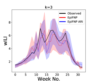
We provided RMSE, LS and CS of AR task in main paper Table 2. See Table 5 for results for AR task that includes MAPE scores. As described in Section 4.2, EpiFNP outperforms baselines in AR tasks and its performance in comparable to EpiFNP scores trained separately for different values of $k$ (Figure 11).

Table 5: Evaluation scores for ARI task (Section 4.2)

	RMSE			MAPE			LS			CS
Model	$k=2$	$k=3$	$k=4$	$k=2$	$k=3$	$k=4$	$k=2$	$k=3$	$k=4$	$k=2$	$k=3$	$k=4$
ED	2.21	3.13	3.82	0.4	0.43	0.55	6.03	8.84	10	0.42	0.45	0.48
MCDP	3.62	4.03	4.39	0.58	0.61	0.67	10	10	10	0.47	0.46	0.49
BNN	3.41	4.23	4.78	0.51	0.55	0.62	10	10	10	0.39	0.41	0.42
GP	1.24	1.31	1.38	0.21	0.21	0.24	4.62	5.17	5.51	0.37	0.36	0.37
EpiFNP	0.6	0.85	0.99	0.1	0.14	0.166	0.64	0.96	1.14	0.063	0.074	0.048

Figure 11: Uncertainty bounds of ARI EpiFNP and normally trained EpiFNP are similar.

Appendix F Ablation study

We examine the effectiveness of three components of EpiFNP in learning accurate predictions and good calibration of uncertainty: (1) Global Latent Variable $\mathbf{v}$ , (2) Local latent variable $\mathbf{z}_{i}^{M}$ (3) Modelling sequence encodings $\mathbf{u_{i}}$ as a random variable instead of directly using deterministic encodings $\bar{\mathbf{h}}_{i}$. Detailed results of this study are in Table 6. All three components are essential for best performance of the model. Removing $\mathbf{z}_{i}^{M}$ shows very large decrease in log scores and calibration scores. This aligns with the hypothesis about role of data correlation graph in determining uncertainty bounds (see Section 4.4).

We present the results of ablation experiments in Table 6. We see that all three components are essential for best performance of the model. Removing $\mathbf{z}^{M}_{i}$ shows large decrease in log scores and calibration scores as the model becomes less capable of modelling uncertainty. Of all the ablation models, making latent embeddings deterministic seems to have least effect on performance though the reduction is still very detrimental to overall performance.

Table 6: Ablation study to measure the effects of 1) Local latent variable $\mathbf{z}_{i}^{M}$ 2) Global latent variable $\mathbf{v}$ and 3) Stochastic SeqEncoder: Modelling $\mathbf{u_{i}}$ as stochastic latent variables rather than deterministic encodings.

Ablation study	RMSE			MAPE
Model/Weeks ahead	2	3	4	2	3	4
EpiFNP	0.48	0.79	0.78	0.089	0.128	0.123
-(Local latent variable)	0.99	1.45	1.51	0.17	0.25	0.29
-(Global latent variable)	1.76	2.05	2.45	0.33	0.41	0.42
- (Stochastic Encoder)	0.87	1.09	1.19	0.15	0.21	0.22
-(Stochastic Encoder, Local latent variable)	1.18	1.39	1.83	0.17	0.18	0.21
- (Stochastic Encoder, Global latent variable)	0.67	0.73	0.9	0.19	0.2	0.26
Ablation study	LS			CS
Model/Weeks ahead	2	3	4	2	3	4
EpiFNP	0.51	0.78	1.2	0.069	0.081	0.035
-(Local latent variable)	3.51	6.67	8.09	0.21	0.27	0.29
-(Global latent variable)	2.06	2.41	3.37	0.085	0.12	0.19
- (Stochastic Encoder)	3.13	3.53	4.88	0.14	0.19	0.24
-(Stochastic Encoder, Local latent variable)	6.11	8.91	9.68	0.44	0.48	0.47
- (Stochastic Encoder, Global latent variable)	2.21	3.58	3.72	0.41	0.45	0.42

Appendix G EpiFNP adapts to H1N1 Flu season

EpiFNP outperforms all baselines and has 30% and 10% better RMSE and MAPE scores compared to second best baseline (RNP). LS of EpiFNP is 0.48, about 9.8 times lesser than second best model. Figure 12(a) shows the prediction and 95% confidence bounds of EpiFNP and two best performing baselines. EpiFNP captures the unprecedented early peak observed around week 4. There is also a high uncertainty bounds around the peak. In contrast RNP has very small uncertainty bounds. GP and most other baselines (except GRU, RNP and MCDP) do not even capture the peak. Calibration plot in Figure 12(b) shows the deviation of EpiFNP from ideal diagonal to be much smaller compared to other baselines. This results in about 4.6 times smaller CS compared to the best baseline.

(a) 2009/10 predictions

(b) 2009/10 Calibration plot

Figure 12: EpiFNP outperforms baselines on real-time forecasting during abnormal H1N1 season (2009/10). Forecasts for $k=3$ weeks ahead forecast by EpiFNP and next two best baselines: RNP and GP.

References

- [1] Bijaya Adhikari, Xinfeng Xu, Naren Ramakrishnan and B. Prakash “EpiDeep: Exploiting Embeddings for Epidemic Forecasting” In Proceedings of the 25th ACM SIGKDD, 2019, pp. 577–586
- [2] Dzmitry Bahdanau, Kyung Hyun Cho and Yoshua Bengio “Neural machine translation by jointly learning to align and translate” In ICLR 2015, 2015
- [3] C. Blundell, Julien Cornebise, K. Kavukcuoglu and Daan Wierstra “Weight Uncertainty in Neural Network” In ICML, 2015
- [4] Logan C. Brooks, David C. Farrow, Sangwon Hyun, Ryan J. Tibshirani and Roni Rosenfeld “Flexible Modeling of Epidemics with an Empirical Bayes Framework” In PLOS Computational Biology, 2015
- [5] Logan C. Brooks, David C. Farrow, Sangwon Hyun, Ryan J. Tibshirani and Roni Rosenfeld “Nonmechanistic forecasts of seasonal influenza with iterative one-week-ahead distributions” In PLOS Computational Biology 14.6, 2018
- [6] Prithwish Chakraborty, Pejman Khadivi and Bryan Lewis et.al “Forecasting a Moving Target: Ensemble Models for ILI Case Count Predictions” In Proceedings of the 2014 SIAM International Conference on Data Mining, Proceedings, 2014, pp. 262–270
- [7] Kyunghyun Cho and Bart Merriënboer et.al “Learning Phrase Representations using RNN Encoder–Decoder for Statistical Machine Translation” In EMNLP, 2014, pp. 1724–1734
- [8] Facebook “The COVID-19 Symptom Data Challenge” In www.symptomchallenge.org, 2020
- [9] Meire Fortunato, Charles Blundell and Oriol Vinyals “Bayesian recurrent neural networks” In arXiv preprint arXiv:1704.02798, 2017
- [10] Yarin Gal and Zoubin Ghahramani “Dropout as a Bayesian Approximation: Representing Model Uncertainty in Deep Learning” In ICML, 2016, pp. 1050–1059
- [11] Marta Garnelo, Jonathan Schwarz, Dan Rosenbaum, Fabio Viola, Danilo J. Rezende, S.. Eslami and Yee Whye Teh “Neural Processes” In Advances in Neural Information Processing Systems 32, 2018
- [12] Chuan Guo, Geoff Pleiss, Yu Sun and Kilian Q Weinberger “On calibration of modern neural networks” In ICML, 2017, pp. 1321–1330
- [13] Herbert W. Hethcote “The Mathematics of Infectious Diseases” In SIAM Review 42.4, 2000, pp. 599–653 DOI: 10.1137/S0036144500371907
- [14] Inga Holmdahl and Caroline Buckee “Wrong but Useful — What Covid-19 Epidemiologic Models Can and Cannot Tell Us” In NEJM 383.4, 2020, pp. 303–305
- [15] Eric Jang, Shixiang Gu and Ben Poole “Categorical Reparameterization with Gumbel-Softmax” In ICLR, 2017
- [16] Michael A Johansson, Karyn M Apfeldorf, Scott Dobson and Jason Devita “An open challenge to advance probabilistic forecasting for dengue epidemics” In Proceedings of the National Academy of Sciences 116.48 National Acad Sciences, 2019, pp. 24268–24274
- [17] Hyunjik Kim, Andriy Mnih, Jonathan Schwarz, Marta Garnelo, Ali Eslami, Dan Rosenbaum, Oriol Vinyals and Yee Whye Teh “Attentive neural processes” In arXiv preprint arXiv:1901.05761, 2019
- [18] Diederik P Kingma and Max Welling “Auto-encoding variational bayes” In ICLR, 2013
- [19] Lingkai Kong, Haoming Jiang, Yuchen Zhuang, Jie Lyu, Tuo Zhao and Chao Zhang “Calibrated Language Model Fine-Tuning For In- And Out-Of-Distribution Data” In Proceedings of the Conference on Empirical Methods in Natural Language Processing, 2020, pp. 1326–1340 DOI: 10.18653/v1/2020.emnlp-main.102
- [20] Lingkai Kong, Haoming Jiang, Yuchen Zhuang, Jie Lyu, Tuo Zhao and Chao Zhang “Calibrated Language Model Fine-Tuning for In- and Out-of-Distribution Data” In Proceedings of the 2020 Conference on Empirical Methods in Natural Language Processing (EMNLP), 2020, pp. 1326–1340 DOI: 10.18653/v1/2020.emnlp-main.102
- [21] Lingkai Kong, Jimeng Sun and Chao Zhang “SDE-Net: Equipping Deep Neural Networks with Uncertainty Estimates” In ICML, 2020, pp. 5405–5415
- [22] Volodymyr Kuleshov, Nathan Fenner and Stefano Ermon “Accurate Uncertainties for Deep Learning Using Calibrated Regression” In Proceedings of the 35th International Conference on Machine Learning, 2018, pp. 2796–2804
- [23] Volodymyr Kuleshov, Nathan Fenner and Stefano Ermon “Accurate uncertainties for deep learning using calibrated regression” In International Conference on Machine Learning, 2018, pp. 2796–2804 PMLR
- [24] Balaji Lakshminarayanan, Alexander Pritzel and Charles Blundell “Simple and scalable predictive uncertainty estimation using deep ensembles” In NeurIPS 2017, 2017, pp. 6405–6416
- [25] Chunyuan Li, Changyou Chen, David Carlson and Lawrence Carin “Preconditioned stochastic gradient Langevin dynamics for deep neural networks” In Proceedings of the AAAI Conference on Artificial Intelligence, 2016
- [26] Christos Louizos, Xiahan Shi, Klamer Schutte and Max Welling “The Functional Neural Process” In Advances in Neural Information Processing Systems 32, 2019, pp. 8746–8757
- [27] Christos Louizos and Max Welling “Multiplicative normalizing flows for variational bayesian neural networks” In arXiv preprint arXiv:1703.01961, 2017
- [28] David JC MacKay “A practical Bayesian framework for backpropagation networks” In Neural computation MIT Press, 1992, pp. 448–472
- [29] Alexandru Niculescu-Mizil and Rich Caruana “Predicting good probabilities with supervised learning” In ICML 2005, 2005, pp. 625–632
- [30] Zhaozhi Qian, Ahmed M Alaa and Mihaela Schaar “When and How to Lift the Lockdown? Global COVID-19 Scenario Analysis and Policy Assessment using Compartmental Gaussian Processes” In Advances in Neural Information Processing Systems 33, 2020
- [31] Shenghao Qin, Jiacheng Zhu, Jimmy Qin, Wenshuo Wang and Ding Zhao “Recurrent Attentive Neural Process for Sequential Data” In arXiv:1910.09323, 2019
- [32] Evan L Ray, Krzysztof Sakrejda, Stephen A Lauer, Michael A Johansson and Nicholas G Reich “Infectious disease prediction with kernel conditional density estimation” In Statistics in medicine 36.30 Wiley Online Library, 2017, pp. 4908–4929
- [33] Evan L Ray, Nutcha Wattanachit and Jarad Niemi “Ensemble Forecasts of Coronavirus Disease 2019 (COVID-19) in the US” In MedRXiv Cold Spring Harbor Laboratory Press, 2020
- [34] Nicholas G. Reich, Logan C. Brooks and Spencer J. Fox “A collaborative multiyear, multimodel assessment of seasonal influenza forecasting in the United States” In PNAS, 2019, pp. 3146–3154
- [35] Hippolyt Ritter, Aleksandar Botev and David Barber “A Scalable Laplace Approximation for Neural Networks” In ICLR, 2018
- [36] Alexander Rodríguez, Nikhil Muralidhar, Bijaya Adhikari, Anika Tabassum, Naren Ramakrishnan and B Aditya Prakash “Steering a Historical Disease Forecasting Model Under a Pandemic: Case of Flu and COVID-19” In Proceedings of the AAAI Conference on Artificial Intelligence 35.6, 2021, pp. 4855–4863
- [37] Alexander Rodríguez, Anika Tabassum, Jiaming Cui, Jiajia Xie, Javen Ho, Pulak Agarwal, Bijaya Adhikari and B Aditya Prakash “DeepCOVID: An Operational Deep Learning-driven Framework for Explainable Real-time COVID-19 Forecasting” In Proceedings of the AAAI Conference on Artificial Intelligence 35.17, 2021, pp. 15393–15400
- [38] Jeffrey Shaman and Alicia Karspeck “Forecasting seasonal outbreaks of influenza” In PNAS 109.50 National Acad Sciences, 2012, pp. 20425–20430
- [39] Hao Song, Tom Diethe, Meelis Kull and Peter Flach “Distribution calibration for regression” In International Conference on Machine Learning, 2019, pp. 5897–5906 PMLR
- [40] Farzaneh Tabataba, Prithwish Chakraborty, Naren Ramakrishnan, Srinivasan Venkatramanan, Jiangzhuo Chen, Bryan Lewis and Madhav Marathe “A framework for evaluating epidemic forecasts” In BMC Inf. Diseases 17.1, 2017, pp. 345
- [41] Ashish Vaswani, Noam Shazeer, Niki Parmar, Jakob Uszkoreit, Llion Jones, Aidan N Gomez, Łukasz Kaiser and Illia Polosukhin “Attention is All you Need” In Advances in Neural Information Processing Systems, 2017, pp. 5998–6008
- [42] Lijing Wang, Jiangzhuo Chen and Madhav Marathe “DEFSI: Deep learning based epidemic forecasting with synthetic information” In Proceedings of the AAAI Conference on Artificial Intelligence 33.01, 2019, pp. 9607–9612
- [43] Ruqi Zhang, Chunyuan Li, Jianyi Zhang, Changyou Chen and Andrew Gordon Wilson “Cyclical Stochastic Gradient MCMC for Bayesian Deep Learning” In ICLR 2020, 2020
- [44] Christoph Zimmer and Reza Yaesoubi “Influenza Forecasting Framework based on Gaussian Processes” In International Conference on Machine Learning, 2020, pp. 11671–11679