Noisy intermediate-scale quantum algorithm for semidefinite programming
Abstract
Semidefinite programs (SDPs) are convex optimization programs with vast applications in control theory, quantum information, combinatorial optimization and operational research. Noisy intermediate-scale quantum (NISQ) algorithms aim to make an efficient use of the current generation of quantum hardware. However, optimizing variational quantum algorithms is a challenge as it is an NP-hard problem that in general requires an exponential time to solve and can contain many far from optimal local minima. Here, we present a current term NISQ algorithm for solving SDPs. The classical optimization program of our NISQ solver is another SDP over a lower dimensional ansatz space. We harness the SDP based formulation of the Hamiltonian ground state problem to design a NISQ eigensolver. Unlike variational quantum eigensolvers, the classical optimization program of our eigensolver is convex, can be solved in polynomial time with the number of ansatz parameters and every local minimum is a global minimum. We find numeric evidence that NISQ SDP can improve the estimation of ground state energies in a scalable manner. Further, we efficiently solve constrained problems to calculate the excited states of Hamiltonians, find the lowest energy of symmetry constrained Hamiltonians and determine the optimal measurements for quantum state discrimination. We demonstrate the potential of our approach by finding the largest eigenvalue of up to dimensional matrices and solving graph problems related to quantum contextuality. We also discuss NISQ algorithms for rank-constrained SDPs. Our work extends the application of NISQ computers onto one of the most successful algorithmic frameworks of the past few decades.
I Introduction
The panorama of quantum computing has been transformed enormously in the last forty years. Once acknowledged as a theoretical pursuit, quantum computers with a few dozen qubits are now a reality. Advancement at the hardware frontier has led to the demonstration of “computational quantum supremacy” for contrived tasks Arute et al. (2019); Zhong et al. (2020). We sit at the edge of the noisy intermediate-scale quantum (NISQ) era Preskill (2018); Bharti et al. (2022). In recent years, significant effort has been put towards designing algorithms for practically relevant tasks which can be implemented on NISQ devices Bharti et al. (2022); Cerezo et al. (2020a). Canonical examples of these NISQ algorithms are variational quantum algorithms (VQAs) such as the variational quantum eigensolver (VQE) Peruzzo et al. (2014); McClean et al. (2016); Kandala et al. (2017) and the quantum approximate optimization algorithm (QAOA) Farhi et al. (2014); Farhi and Harrow (2016). NISQ algorithms have been developed for various tasks such as finding the ground state of Hamiltonians Peruzzo et al. (2014); McClean et al. (2016); Kandala et al. (2017); McClean et al. (2017); Kyriienko (2020); Parrish and McMahon (2019); Bespalova and Kyriienko (2020); Huggins et al. (2020); Takeshita et al. (2020); Stair et al. (2020); Motta et al. (2020); Seki and Yunoki (2021); Bharti (2020); Bharti and Haug (2021a); Cervera-Lierta et al. (2021), combinatorial optimization Farhi et al. (2014); Farhi and Harrow (2016), quantum simulation Li and Benjamin (2017); Yuan et al. (2019); Benedetti et al. (2020); Bharti and Haug (2021b); Barison et al. (2021); Commeau et al. (2020); Heya et al. (2019); Cirstoiu et al. (2020); Gibbs et al. (2021); Lau et al. (2021a); Haug and Bharti (2020); Otten et al. (2019); Lim et al. (2021); Lau et al. (2021b) quantum metrology Meyer et al. (2021); Meyer (2021) and machine learning Schuld and Killoran (2019); Havlíček et al. (2019); Kusumoto et al. (2019); Farhi and Neven (2018); Mitarai et al. (2018). These algorithms have been investigated in detail with a comprehensive exposition on possible hurdles McClean et al. (2018); Sharma et al. (2020); Cerezo et al. (2020b); Wang et al. (2021); Bittel and Kliesch (2021); Huang et al. (2021) and corresponding countermeasures Huang et al. (2021); Haug et al. (2021); Haug and Kim (2021); Larocca et al. (2021a). A thorough study of possible applications of NISQ devices is expected to unravel the potential as well as limitations of such devices. Moreover, in the quest for practical quantum advantage in the NISQ era it is pertinent to investigate novel NISQ algorithms for practically relevant tasks.
A major challenge in the NISQ era is the optimization program for VQAs, where a classical optimizer is searching for the parameters of a quantum state that minimizes a cost function. For the VQA to be successful, one requires an ansatz that is expressible enough to approximate the optimal solution of the corresponding optimization problem. However, even if such ansatz has been found, the optimization program of the VQA is NP-hard and in contrast to classical neural networks the optimization landscape contains numerous far from optimal local minima Bittel and Kliesch (2021); Anschuetz (2021); You and Wu (2021). The highly non-convex nature of landscape renders optimization difficult even for VQAs involving logarithmically many qubits or classically easy problems such as free fermions. Further, VQAs struggle to optimize problems where the solution space is constrained due to symmetries such as for chemistry problems Higgott et al. (2019); McClean et al. (2016); Rubin et al. (2018); Ryabinkin et al. (2018); Greene-Diniz and Muñoz Ramo (2021); Kuroiwa and Nakagawa (2021).
In the last few decades, semidefinite programs (SDPs) have led to ground breaking developments in mathematical optimization Vandenberghe and Boyd (1996); Wolkowicz et al. (2012). The study of SDPs has uncovered numerous applications in theoretical computer science, control theory and operations research. Many problems in quantum information such as state discrimination Skrzypczyk et al. (2019); Bae and Kwek (2015); Ježek et al. (2002), dimension witness Ray et al. (2021) and self-testing Bharti et al. (2019a, b, 2021); Yang et al. (2014); Bancal et al. (2015) can be investigated using SDPs. While SDPs can be solved efficiently in polynomial time on classical computers, high dimensional problems may still be out of scope for classical computers. For example, finding the ground state of a Hamiltonian can be framed as a SDP, however it is intractable for classical computers due to the exponential scaling of the dimension of the problem. To explore possible quantum advantages for solving SDPs with quantum computers, quantum SDP solvers have been studied comprehensively Brandão et al. (2017); Van Apeldoorn et al. (2017); van Apeldoorn and Gilyén (2018); Kerenidis and Prakash (2020); Brandao and Svore (2017); Chakrabarti et al. (2020); van Apeldoorn et al. (2018). However, existing quantum SDP solvers cannot be executed on NISQ devices as they require extensive quantum resources.
Here, we propose the NISQ SDP Solver (NSS) as a hybrid quantum-classical algorithm to solve SDPs. The NSS encodes a SDP onto a quantum computer combined with an optimization routine on a classical computer. The classical optimization part of the NSS is also a SDP with its dimension given by the size of the ansatz space. The quantum computational part of the NSS has no classical-quantum feedback loop and requires the quantum computer only for estimating overlaps, which can be done efficiently on current NISQ devices. We showcase the NSS for a wide range of problems. We design a NISQ SDP based quantum eigensolver (NSE) to find the ground state of quantum Hamiltonians. In contrast to VQE, the classical optimization part of the NSE can be solved in polynomial time without the local minima problem. We find numerical evidence that the NSE improves the estimation of the ground state energy by a constant factor for any number of qubits for a non-integrable one-dimensional Ising model combined with a quantum annealing ansatz. Furthermore, the NSS is capable of efficiently implementing constraints in the optimization program in order to calculate excited states and solve symmetry constrained problems. In addition, we provide an NSS for determining optimal measurements for quantum state discrimination. The NSS can be also find the largest eigenvalue of matrices, which we demonstrate for matrices as large as . Finally, we show the NSS for various important problems related to quantum information such as Bell non-local games and the Lovász Theta number. We also provide the extension of the NSS for rank-constrained SDPs.
One can argue that SDPs are solvable efficiently in polynomial time on classical computers and hence why should one construct a NISQ algorithm for SDPs. We would like to stress that the polynomial runtime is in terms of the input matrix size and the number of constraints. For problems with exponential input size, polynomial of exponential would be still exponential and hence classical SDPs would be unable to process such cases. To begin, the Hamiltonian ground state problem is an SDP, but that does not mean it is tractable. In other words, while SDPs can be solved in polynomial time and memory, when the problem scales exponentially classical computers are unable to process it. For example, no classical computer in the world is able to store a problem of size . However, quantum computers can store this vector efficiently within a quantum state of 60 qubits, which is the current state of the art of NISQ computers. Here, our NSS algorithm offers the potential to outperform any classical SDP solver.
II Background
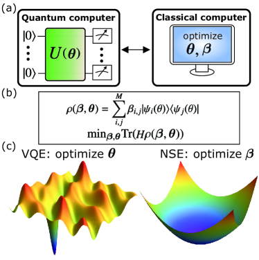
We now highlight the key difference between VQA and NSS in Fig.1 by using the ground state problem as an example. Finding the ground state of a Hamiltonian can be framed as a SDP using density matrices (see program 10), however the SDP suffers from exponential scaling of the dimension of the quantum state and thus it is difficult to solve on classical computers. To address the scaling of the quantum state, VQE and NSE map the quantum state onto a quantum computer. VQE uses a quantum circuit parameterized by the parameter . Then, the VQE minimizes the energy of the quantum state by variationally adjusting the parameter via a classical optimization routine in a feedback loop. However, this minimization task is challenging as the corresponding optimization program is non-convex and NP-hard Bittel and Kliesch (2021). In contrast to classical neural networks, the optimization landscape of VQEs is characterised by local minimas far from the global minima, where optimization routines are unlikely to find reasonable approximations of the global minima Anschuetz (2021). Only for overparameterized circuits the landscape becomes favorable, which for most types of circuits requires an exponential amount of parameters and exponentially deep circuits Larocca et al. (2021b); Haug et al. (2021).
In contrast, the NSS uses a hybrid density matrix Eq. (4). It consists of a linear combination of a -dimensional set of ansatz quantum states with classical combination coefficients . In the NSS, the parameters are optimised to minimize the energy. The optimization of the coefficients is another SDP with dimension only, which can be efficiently optimised in polynomial time on a classical computer. The ansatz preserves the convexity of the landscape and hence any local minimum is also a global minimum.

III Semidefinite Program
SDPs can be thought of as generalization of the “standard form” linear programming (LP). The “standard form” of LP is given by
| (1) | |||
where the set is given by . Here, . The set is known as nonnegative orthant. The phrase “standard form” hints that there are other possible non-standard representations of LPs. Any LP in non-standard form, however, can be converted into standard form by following a few tricks. These tricks include change of variables, transforming the inequalities into equalities and switching maximum to minimum.
In a SDP, the non-negativity constraint is replaced by positive semidefinite cone constraint SDPs involve optimization of a linear function of matrix over the affine slice of the cone of positive semidefinite matrices. The standard form of a SDP is given by
| (2) | |||
Here, denotes the set of symmetric positive semidefinite matrices. Mathematically speaking, . The matrices and belong to the set of symmetric matrices for . The -th element of vector is denoted by .
Duality is one of the oldest and most fruitful ideas in mathematics. The duality principle of mathematical optimization theory suggests that mathematical optimization problems can be viewed from either of two perspectives, namely the primal problem or the dual problem. For a given primal minimization problem , the solution to the corresponding dual problem problem provides a lower bound to the solution of . The standard form of the dual of the SDP in program 2 is given by
| (3) | |||
The SDPs in programs 2 and 3 constitute a primal-dual pair. SDPs can be extended to complex-valued matrices via a cone of Hermitian positive semidefinite matrices i.e. . Here, denotes the set of Hermitian positive semidefinite matrices. Since SDPs for complex-valued matrices are more general than SDPs for real valued matrices, we will consider the former case in this work.
IV The NSS
We now outline the NSS, which consists of three distinct steps, namely ansatz selection, overlap measurement and post-processing. First, we select a set of quantum states over a Hilbert space , where the set contains quantum states . Now, our NISQ semidefinite programming solver (NSS) uses the following hybrid density matrix ansatz
| (4) |
where . Note that the quantum states in are prepared by a quantum system while the coefficients are stored on some classical device as matrix . For , we have (see Appendix B). We now assume that and constraint matrices of program 2 can be written as a sum of unitaries
As second step of the NSS, we measure the following overlaps on the quantum system
| (5) | |||
| (6) |
The overlaps can be measured using the Hadamard test or with direct measurement methods Mitarai and Fujii (2019). An alternative NISQ-friendly method that requires only sampling in the computational basis has been proposed in Bharti and Haug (2021a), which we use in the following. This method assumes that the unitaries and are Pauli strings with . As the Pauli strings form a complete basis, any matrix can be decomposed into a linear combination of Pauli strings. Further, we assume that the ansatz space is generated by an initial state and a set of different Pauli strings via . Now, each overlap element in Eq. (5), Eq. (6) can be written as a sum of expectation values of Pauli strings , where we use that a product of Pauli strings can be written as a single Pauli string with a prefactor . Then, one can efficiently calculate the overlap elements by measuring the expectation values of Pauli strings. On NISQ computers, this can be done by preparing the initial state , performing single-qubit rotations into the eigenbasis of the Pauli operator and then sampling in the computational basis times. We note that sampling from quantum circuits is general intractable for classical computers Aaronson and Chen (2016). The additive error of estimating the expectation value of Pauli strings scales as according to Hoeffding’s inequality and is independent of the number of qubits Huang et al. (2021).
The third and final step of the NSS consists of post-processing on a classical computer. Here, we write the standard form primal SDP in terms of the measured overlaps
| (7) | |||
This is a SDP over with the corresponding hybrid density matrix is given by Eq. (4). The dual of the SDP in program 7 is given by
| (8) | |||
The SDPs in program 7 and 8 constitute a primal-dual pair over the ansatz space that can be solved in polynomial time on a classical computer. In the case where the ansatz states are linear independent and cover the whole Hilbert space, the programs 7 and 8 over the ansatz space recover the SDPs over the entire space corresponding to programs 2 and 3.
V Extensions to Rank-constrained SDPs
Rank constrained SDPs find numerous applications in combinatorics Marianna et al. (2013), control theory Boyd et al. (1994) and quantum information Ray et al. (2021). Many problems in optimization theory can be modelled as rank-constrained SDPs Vandenberghe and Boyd (1996); Anjos and Lasserre (2011). The rank-constraint turns the optimization program into a non-convex and NP-hard problem, which is in general intractable to solve. The optimization program for rank constrained SDPs is given by
| (9) | |||
Notice that the only difference between the regular SDP in program 2 and the rank-constrained SDP in program 9 is the presence of the rank constraint in the latter. Intuitively speaking, the aforementioned rank constraint means that the optimizer of the program 9 must have a rank of at most . The famous Max-Cut problem can be modelled as a rank constrained SDP for (see Appendix C). We defer the extension of the NSS for the rank constrained SDPs in Appendix C.
VI Examples
We now demonstrate the NSS for various problems of interest.
VI.1 Ground State Problem
First, we demonstrate the NSE solver to find the ground state of Hamiltonians. For Hamiltonian and density matrix , the problem of finding the ground state can be written as
| (10) | |||
The dual formulation for Program 10 is given by
| (11) | |||
The optimum value of corresponds to the ground state energy. In the ansatz space generated by , the primal SDP for the Hamiltonian ground state problem is given by
| (12) | |||
with and . The dual program of Program 12 is given by
| (13) | |||
Notice that the primal optimization program over is convex and hence exhibits a unique minimum value. This is unlike the case of VQE, where optimization is non-convex and there can be multiple local minima Bittel and Kliesch (2021). In the NSE, the classical optimization finds the optimal solution in time polynomial in the number of ansatz parameters, given that the solution is contained in the ansatz space. On the other hand, in VQAs such as VQE and QAOA, even if the optimal solution is contained in the ansatz space, the classical optimization can be NP-hard Bittel and Kliesch (2021). Moreover, the primal optimal solution is equal to the dual optimal solution.
Claim 1.
Proof.
To show that the SDP in Program 12 admits strong duality, we need to show that the interior is non-empty Boyd and Vandenberghe (2004). The non-empty interior can be established via the existence of a full rank feasible solution for Program 12. Consider
Clearly, is feasible and full rank. This completes the proof. ∎
Now we demonstrate the NSE for finding the ground state of a non-integrable model, namely the one-dimensional Ising model of qubits with transverse field and longitudinal field
| (14) |
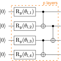
with and . First, we prepare an initial state on the quantum computer, which we then use to construct the ansatz space. As initial state, we either choose a hardware efficient circuit consisting layers of randomized -rotations and CNOT gates arranged in a chain topology (see Appendix A) , a product state and a discretized quantum annealing state
| (15) |
where is the number of layers of the circuit and the quantum annealing time. The state is constructed by evolving with Eq. (14), where we stepwise evolve with the non-commuting parts and . This state is a discretized form of a quantum annealing protocol, where one starts with the ground state of , and then slowly increases until one reaches the target Hamiltonian Eq. (14). In the limit , the adiabatic theorem guarantees that this state becomes the exact ground state Kadowaki and Nishimori (1998). A similar type of ansatz with additional variational parameters is used for QAOA and VQE Farhi et al. (2014); Wiersema et al. (2020).
To generate the ansatz space for Eq. (4), we use a NISQ-friendly adaption of the Krylov subspace approach Lanczos (1950); Saad (1992); Seki and Yunoki (2021); Motta et al. (2020). In the original Krylov subspace approach, the ground state is approximated by a sum of powers of the Hamiltonian applied on the initial state prepared on the quantum computer with appropriate coefficients and truncated up to order
| (16) |
However, on NISQ computers it is challenging to measure . To simplify this approach, we use the fact that the Ising Hamiltonian is a sum of Pauli strings . We decompose the power of the Hamiltonian into a sum of products of Pauli strings. We then take each product of Pauli string and add each unique term to the set Bharti and Haug (2021a). Note that a product of Pauli strings is again a Pauli string. We do this for each power of the Hamiltonian up to order . The generated set contains the original Krylov subspace. However, it can be easily measured on NISQ devices as the corresponding overlaps are simple measurements of Pauli strings. We show as example the first order of the ansatz states for Eq. (14) with states
We use a subset of states from to run the NSE and investigate the convergence of our approach, where we select the first states in ascending order of the order of the Krylov subspace .
 (a)
(a)
 (b)
(b)
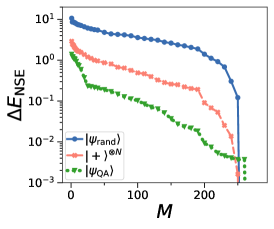
In Fig.2a, we investigate the error between the energy via the NSE and the exact ground state energy as function of . We find that with increasing the energy decreases and beyond a threshold the exact ground state is reached. The quality of the approximation highly depends on the choice of initial state. We find that the random circuit state converges slowly and only finds the exact ground state when becomes the same order as the Hilbert space, In contrast, the quantum annealing state converges much faster to a small error and yields a good approximation of the energy even at modest .
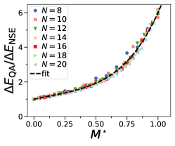
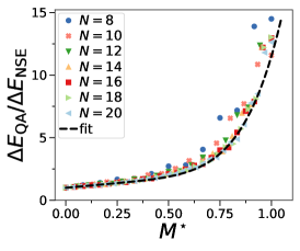
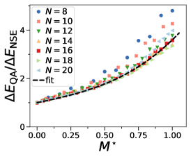
In Fig.2b, we investigate the scaling of the NSE with number of qubits . We prepare the quantum annealing ansatz with layers with energy . Now, we apply the NSE with initial state to improve the energy estimation by using the first order of the NISQ-friendly Krylov subspace Eq. (16). We show the improvement of NSE in estimating the energy relative to the error of quantum annealing . With increasing number of ansatz states , improves non-linearly. For any number of qubits, collapses to a single curve as function of number of ansatz states normalised by the number of qubits . This suggests that we can achieve a scalable improvement in energy estimation when the number of ansatz states scales linearly with . For example, we achieve a factor of 6 improvement for ansatz states for any . This demonstrates that the NSE can substantially enhance the accuracy of finding the ground state energy even for larger system sizes. In the Appendix E, we show that the same scaling appears for different parameters of the Hamiltonian and the quantum annealing state.
VI.2 Excited states
We now adapt the NSS solver to find the excited states of the Hamiltonian. We assume that we already found approximations for ground state and the first first excited states with the coefficients , . To find the excited state with coefficient , we run the NSS with the added constraint that the overlap between and the already found states is zero with . The state with the smallest energy that satisfies the constraints is the approximation of the excited state. The NSS solver for excited states is given by
| (17) | |||
We can be run Program 17 iteratively with the output of the previous iterations to find up to excited states.
VI.3 Symmetry-resolved lowest eigenenergy
Quantum many-body Hamiltonians often have symmetries. Each symmetry corresponds to a particular symmetry operator which commutes with the Hamiltonian . Under time evolution with , the expectation value of is conserved. A common task encountered in quantum many-body physics and quantum chemistry is to find the eigenstate with lowest energy that is simultaneously an eigenstate of the symmetry with a conserved quantity . One common approach to solve this problem is use an ansatz that respects the symmetry operator initialised with the desired Gard et al. (2020); Kokail et al. (2019). However, finding such an ansatz can be difficult and the optimisation is more challenging compared to a general ansatz that breaks the symmetry Choquette et al. (2021); Kokail et al. (2019). Another approach is to add penalty terms to the Hamiltonian, but this is known to render the optimization far more challenging Higgott et al. (2019); Kuroiwa and Nakagawa (2021).
Our SDP solver opens up a new way to find the lowest eigenenergy with the conserved quantity. We constrain the minimization problem of the Hamiltonian to the subspace where takes the eigenvalue
| (18) | |||
Here, we demand that the expectation value of the symmetry operator and its square are fixed to the conserved quantity, i.e. and . Here, is needed to make sure that we find an eigenstate of the symmetry operator. We now give the corresponding formulation as NSS
| (19) | |||
Here, we define and , where and can be decomposed into a sum of unitaries. In contrast to VQE, SDPs with constraints are convex and can be efficiently solved.
We implement our solver for two important quantum many-body problems, the transverse Ising model Eq. (14) and the Heisenberg model
| (20) |
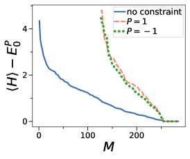
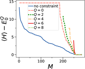
As demonstration, for the transverse Ising model () we consider its parity symmetry with conserved quantities . For the Heisenberg model, we consider the conservation of number of particles with . We run the NSS with a random hardware efficient circuit and the NISQ-friendly adaption of the Krylov subspace approach to construct the ansatz states. In Fig.3 we solve for the lowest eigenenergy within a particular symmetry sector for varying number of ansatz states . For low , the constrained NSE does not find any solution as the ansatz is unable to satisify the constraints for the symmetry. Above a specific , we find an appropriate solution, which for further increase of converges to the lowest eigenenergy for the given conserved quantity. For the Heisenberg model, we find that higher particles require a larger number of ansatz states to find a feasible solution. We believe that by replacing the random hardware efficient circuit with a better suited initial state, the convergence of the energy can be tremendously improved.
 (a)
(a)
 (b)
(b)
VI.4 Largest Eigenvalue
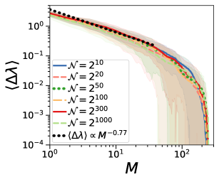
Our next task is to find the largest eigenvalue of a sparse matrix by maximizing Program 12. We assume that is of size and is represented by a combination of Pauli string , where the Pauli strings are given by with and is a prefactor. To numerically demonstrate the performance of NSS, we uniformly sample the Pauli operators for each qubit, choose random and use the -bit state with all zeros as ansatz state. Using the Krylov subspace idea for finding the ground state, we similarly construct the ansatz space . While the expectation values can be calculated classically for the product state, it becomes an intractable problem when using highly entangled quantum states as ansatz states. In Fig.4, we plot the difference between the largest eigenvalue found by NSE and the exact solution as function of the number of states within the ansatz space for different matrix dimensions . For small , we find that the error decreases approximately with . Beyond a threshold , we find very good convergence even for matrix dimensions .

VI.5 Unambiguous state discrimination
The task of state discrimination is to identify states drawn randomly from a set by performing a measurement on the state. General measurements are described by positive operator-valued measures (POVMs) with the condition . If all the states are pure and pairwise orthogonal, one can simply measure with the projectors on the individual states . However, for non-orthogonal states this naive approach will result in classification errors. However, we can find a set of POVMs that can unambiguously classify pure states. The POVMs are of the form with . When we measure the outcome associated to POVM with probability , we classify the measured state as . If we measure the outcome with POVM , then we say that we are unable to classify the state. The problem of finding the optimal set of POVMs can be formulated as an SDP. Our goal is to optimize POVMs in respect to the average probability to correctly classify the states. Further, we demand that the probability of wrongly classifying state is bounded by , with . The SDP is given by
| (21) | |||
We can formulate the problem as a NSS. We assume we are given a set of states to be discriminated written in the form of hybrid states with the matrix and ansatz states . To get valid density matrices, we have , and . We write the POVMs to be optimized as hybrid POVMs
| (22) |
with . The last POVM for the case where we are unable to classify the state is given by . We demand that is positive semidefinite, which is always fulfilled when . is positive semidefinite when for any state we have . We can write arbitrary states as with state being orthogonal to the subspace spanned by the ansatz states and normalised coefficients , . A straightforward calculation shows , which is non-negative when . The program of the NSS for state discrimination is now given by
| (23) | |||
As both the states and POVMs are constructed from the same ansatz space, it is unsurprising that Program 23 finds the optimal POVMs for unambiguous state discrimination for any number of qubits.
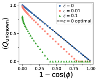
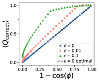
We demonstrate in Fig.5 our algorithm by classifying two pure states generated by a hardware efficient quantum circuit (see Appendix A), which is intractable to simulate for large number of qubits. The two states and are prepared as where are a random set of Pauli strings. The matrix can be efficiently measured on NISQ computers as shown in Sec. IV. In Fig.5a, we show the probability of correctly identifying the states as function of the angle between the two states. We find that for demanding zero misclassification error , our NSS finds the analytically known optimal POVMs with Peres (1988). In Fig.5b, we show the average probability that we cannot make a decision. The change in slope of the classification probability for seen in Fig.5a coincides with .
 (a)
(a)  (b)
(b)
VI.6 Lovász Theta Number
Graph invariants are properties that depend only on the abstract structure of a graph. The Lovász Theta number is such a graph invariant that was first introduced by László Lovász in the breakthrough paper titled “On the Shannon capacity of a Graph” Lovász (1979). The Lovász Theta number provides an upper bound to the Shannon capacity of a graph, another graph invariant quantity. Surprisingly, it is connected with quantum contextuality Budroni et al. (2021); Cabello et al. (2014); Bharti et al. (2020, 2019b, 2019a, 2021) and can help us to understand the potential of quantum computers Howard et al. (2014). Given a graph with vertex set and adjacency matrix , the SDP for the Lovász Theta number is given by
| (24) | |||
Here, is an all one matrix. Since is real valued, the ansatz space can be taken as real valued, which can be achieved within NSS by demanding that the ansatz quantum states are real valued.
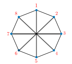
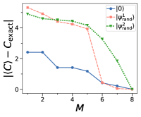
To demonstrate the NSS, we calculate the Lovász Theta number for the graph shown in Fig. 6. To generate the ansatz states , we apply a set of Pauli operators on a quantum state. We use the zero state or representative examples of randomized states generated via hardware efficient quantum circuits (see Appendix A). Then, the set of basis states is generated by applying different combinations of Pauli strings on the state , where with . In Fig.7a we show the error of the NSS. We calculate the error as the difference between the exact solution , including the constraints of the problem, and the expectation values gained from the quantum state via NSS. We observe an improvement with increasing number of ansatz states , reaching the optimal solution latest when the number of basis states reaches the dimension of the problem. Depending on the choice of initial state, the optimal solution can be reached with a lower number of ansatz states.
 (a)
(a) 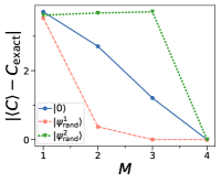 (b)
(b)
VI.7 Bell Non-Locality
Finally we apply the NSS to calculate the quantumly achievable success probability for the canonical Bell non-local game: the Clauser Horn Shimony Holt (CHSH) game Bell (1964); Clauser et al. (1969); Brunner et al. (2014); Scarani (2019). The CHSH game involves two spacelike separated parties, say Alice and Bob. A referee asks the players uniformly random pairs of questions . The players have to answer such that
| (25) |
Here denotes addition modulo and is the logical AND operator. Using classical strategies, the maximum probability of success for the CHSH game is upper bounded by . However, using quantum resources such as entangled states, the players can win the game with probability . The success probability for the CHSH game can be calculated using a SDP. For details, see Appendix D. We implemented the aforementioned SDP using NSS in Fig.7b using the same ansatz as for the Lovász Theta number and find that for sufficient number of basis states we achieve the correct result.
VII Conclusion
We presented the NSS for solving SDPs, including rank-constrained SDPs. Our algorithm runs on NISQ devices without the need for classical-quantum feedback loops, requiring only the measurement of overlaps on the quantum computer. When the ansatz space is generated by expanding an initial state with Pauli strings, these overlaps can be measured by sampling the initial state in a Pauli rotated basis (see Sec.IV).
The ground state problem expressed in terms of density matrices is a SDP and hence a convex optimization program. However, the SDP corresponding to the ground state problem suffers from exponential scaling of the dimension of the quantum state, rendering it difficult to solve on classical computers. To tackle the exponential scaling of the dimension, VQEs employ optimization over smaller dimensional ansatz space. However, the classical optimization corresponding to VQEs is NP-hard, and the landscape contains numerous far from optimal persistent local minima Bittel and Kliesch (2021); Anschuetz (2021); You and Wu (2021). We employed our NSS to develop the NSE, a NISQ algorithm for the ground state problem. The key idea of our NSE is to optimize over a smaller number of parameters while preserving the convexity of the original problem. Unlike VQEs, our optimization program is convex, and thus every local minimum is a global minimum. Moreover, the classical optimization program of the NSE is a SDP that can be solved in polynomial-time. Further, our NSS can efficiently implement constraints on the solution space, which is a well known challenge for VQAs Kuroiwa and Nakagawa (2021).
The previously proposed quantum assisted eigensolver and iterative quantum assisted eigensolvers Bharti (2020); Bharti and Haug (2021a) are special cases of our rank constrained SDP solver with unit rank (see Appendix C). With our NSS, it is now possible to solve many important problems that can be formulated in terms of SDPs in a NISQ setting. Our work unlocks the possibility of running one of the most important algorithmic frameworks of classical computing on NISQ computers and exploring the capabilities of the current generation quantum computers. We can use it to find approximation of the ground state and excited states of Hamiltonians, as well as solve symmetry constrained problems. Further, we show how to use NISQ computers to find POVMs that unambiguously discriminate states. We also implemented the NSS to calculate Lovász Theta number, a graph invariant with various applications, including in quantum contextuality. Further, we used our algorithm to determine the maximum winning probability of Bell nonlocal games. We demonstrated the applicability of our algorithm for finding the largest eigenvalue of dimensional matrices. In a recent work Yu et al. (2022), it was shown that a large family of rank- constrained SDPs can be written as a convex optimization over separable two-party quantum states. To solve the aforementioned convex optimization problems, Yu et al. (2022) provides a complete hierarchy of SDPs. Based on this result and the techniques in our paper, one can solve the rank-constrained NISQ SDP with a hierarchy of NISQ SDPs.
Our work leads to many novel avenues for future research. Investigating a systematic problem aware strategy for determining the initial state and the set of basis states used to construct the hybrid density matrix will help improve as well as understand the NSS and its rank constrained variants. It would be fascinating to study our algorithms in the presence of noise Epperly et al. (2021). Further, analysing our algorithms to render complexity-theoretic statements is another exciting direction for further investigation.
The ground state problem can be thought of as quantum native problem in the sense that the exponential scaling of the Hilbert space size makes it challenging to solve with classical devices. This problem can be framed as a convex optimization program over density matrices. Thus, we could conceive the ground state problem as a “convex quantum native problem”. In future, it would be interesting to employ techniques from our work to other convex quantum native problems from disciplines such as quantum chemistry, condensed matter physics and quantum information. As we numerically find a clear scaling law in number of qubits for the NSE, we believe rigorous guarantees for the performance of our algorithm for large system sizes can be proven.
The Quantum interior-point method Kerenidis and Prakash (2020) and quantum multiplicative weight approaches Brandão et al. (2017); Van Apeldoorn et al. (2017); van Apeldoorn and Gilyén (2018) have been proposed in the literature to solve SDPs. It would be interesting to develop the corresponding NISQ algorithms. Extending our work to the general case of cone programming seems another exciting direction.
Python code for the numerical calculations performed are available at Haug and Bharti .
Acknowledgements— We thank Atul Singh Arora for interesting discussions. We are grateful to the National Research Foundation and the Ministry of Education, Singapore for financial support.
References
- Arute et al. (2019) F. Arute, K. Arya, R. Babbush, D. Bacon, J. C. Bardin, R. Barends, R. Biswas, S. Boixo, F. G. Brandao, D. A. Buell, et al., Nature 574, 505 (2019).
- Zhong et al. (2020) H.-S. Zhong, H. Wang, Y.-H. Deng, M.-C. Chen, L.-C. Peng, Y.-H. Luo, J. Qin, D. Wu, X. Ding, Y. Hu, et al., Science 370, 1460 (2020).
- Preskill (2018) J. Preskill, Quantum 2, 79 (2018).
- Bharti et al. (2022) K. Bharti, A. Cervera-Lierta, T. H. Kyaw, T. Haug, S. Alperin-Lea, A. Anand, M. Degroote, H. Heimonen, J. S. Kottmann, T. Menke, W.-K. Mok, S. Sim, L.-C. Kwek, and A. Aspuru-Guzik, Rev. Mod. Phys. 94, 015004 (2022).
- Cerezo et al. (2020a) M. Cerezo, A. Arrasmith, R. Babbush, S. C. Benjamin, S. Endo, K. Fujii, J. R. McClean, K. Mitarai, X. Yuan, L. Cincio, et al., arXiv preprint arXiv:2012.09265 (2020a).
- Peruzzo et al. (2014) A. Peruzzo, J. McClean, P. Shadbolt, M.-H. Yung, X.-Q. Zhou, P. J. Love, A. Aspuru-Guzik, and J. L. Obrien, Nature communications 5, 4213 (2014).
- McClean et al. (2016) J. R. McClean, J. Romero, R. Babbush, and A. Aspuru-Guzik, New Journal of Physics 18, 023023 (2016).
- Kandala et al. (2017) A. Kandala, A. Mezzacapo, K. Temme, M. Takita, M. Brink, J. M. Chow, and J. M. Gambetta, Nature 549, 242 (2017).
- Farhi et al. (2014) E. Farhi, J. Goldstone, and S. Gutmann, arXiv:1411.4028 (2014).
- Farhi and Harrow (2016) E. Farhi and A. W. Harrow, arXiv preprint arXiv:1602.07674 (2016).
- McClean et al. (2017) J. R. McClean, M. E. Kimchi-Schwartz, J. Carter, and W. A. De Jong, Physical Review A 95, 042308 (2017).
- Kyriienko (2020) O. Kyriienko, npj Quantum Information 6, 1 (2020).
- Parrish and McMahon (2019) R. M. Parrish and P. L. McMahon, arXiv preprint arXiv: 1909.08925 (2019).
- Bespalova and Kyriienko (2020) T. A. Bespalova and O. Kyriienko, arXiv preprint arXiv:2009.03351 (2020).
- Huggins et al. (2020) W. J. Huggins, J. Lee, U. Baek, B. O’Gorman, and K. B. Whaley, New Journal of Physics (2020).
- Takeshita et al. (2020) T. Takeshita, N. C. Rubin, Z. Jiang, E. Lee, R. Babbush, and J. R. McClean, Physical Review X 10, 011004 (2020).
- Stair et al. (2020) N. H. Stair, R. Huang, and F. A. Evangelista, Journal of Chemical Theory and Computation 16, 2236 (2020).
- Motta et al. (2020) M. Motta, C. Sun, A. T. Tan, M. J. O’Rourke, E. Ye, A. J. Minnich, F. G. Brandão, and G. K.-L. Chan, Nature Physics 16, 205 (2020).
- Seki and Yunoki (2021) K. Seki and S. Yunoki, PRX Quantum 2, 010333 (2021).
- Bharti (2020) K. Bharti, arXiv preprint arXiv:2009.11001 (2020).
- Bharti and Haug (2021a) K. Bharti and T. Haug, Physical Review A 104, L050401 (2021a).
- Cervera-Lierta et al. (2021) A. Cervera-Lierta, J. S. Kottmann, and A. Aspuru-Guzik, PRX Quantum 2, 020329 (2021).
- Li and Benjamin (2017) Y. Li and S. C. Benjamin, Physical Review X 7, 021050 (2017).
- Yuan et al. (2019) X. Yuan, S. Endo, Q. Zhao, Y. Li, and S. C. Benjamin, Quantum 3, 191 (2019).
- Benedetti et al. (2020) M. Benedetti, M. Fiorentini, and M. Lubasch, arXiv preprint arXiv:2009.12361 (2020).
- Bharti and Haug (2021b) K. Bharti and T. Haug, Phys. Rev. A 104, 042418 (2021b).
- Barison et al. (2021) S. Barison, F. Vicentini, and G. Carleo, Quantum 5, 512 (2021).
- Commeau et al. (2020) B. Commeau, M. Cerezo, Z. Holmes, L. Cincio, P. J. Coles, and A. Sornborger, arXiv:2009.02559 (2020).
- Heya et al. (2019) K. Heya, K. M. Nakanishi, K. Mitarai, and K. Fujii, arXiv preprint arXiv:1904.08566 (2019).
- Cirstoiu et al. (2020) C. Cirstoiu, Z. Holmes, J. Iosue, L. Cincio, P. J. Coles, and A. Sornborger, npj Quantum Information 6, 1 (2020).
- Gibbs et al. (2021) J. Gibbs, K. Gili, Z. Holmes, B. Commeau, A. Arrasmith, L. Cincio, P. J. Coles, and A. Sornborger, arXiv preprint arXiv:2102.04313 (2021).
- Lau et al. (2021a) J. W. Z. Lau, K. Bharti, T. Haug, and L. C. Kwek, arXiv preprint arXiv:2101.07677 (2021a).
- Haug and Bharti (2020) T. Haug and K. Bharti, arXiv preprint arXiv:2011.14737 (2020).
- Otten et al. (2019) M. Otten, C. L. Cortes, and S. K. Gray, arXiv preprint arXiv:1910.06284 (2019).
- Lim et al. (2021) K. H. Lim, T. Haug, L. C. Kwek, and K. Bharti, Quantum Science and Technology 7, 015001 (2021).
- Lau et al. (2021b) J. W. Z. Lau, T. Haug, L. C. Kwek, and K. Bharti, arXiv preprint arXiv:2103.05500 (2021b).
- Meyer et al. (2021) J. J. Meyer, J. Borregaard, and J. Eisert, npj Quantum Information 7, 1 (2021).
- Meyer (2021) J. J. Meyer, arXiv preprint arXiv:2103.15191 (2021).
- Schuld and Killoran (2019) M. Schuld and N. Killoran, Phys. Rev. Lett. 122, 040504 (2019).
- Havlíček et al. (2019) V. Havlíček, A. D. Córcoles, K. Temme, A. W. Harrow, A. Kandala, J. M. Chow, and J. M. Gambetta, Nature 567, 209 (2019).
- Kusumoto et al. (2019) T. Kusumoto, K. Mitarai, K. Fujii, M. Kitagawa, and M. Negoro, arXiv:1911.12021 (2019).
- Farhi and Neven (2018) E. Farhi and H. Neven, arXiv:1802.06002 (2018).
- Mitarai et al. (2018) K. Mitarai, M. Negoro, M. Kitagawa, and K. Fujii, Physical Review A 98, 032309 (2018).
- McClean et al. (2018) J. R. McClean, S. Boixo, V. N. Smelyanskiy, R. Babbush, and H. Neven, Nature communications 9, 4812 (2018).
- Sharma et al. (2020) K. Sharma, M. Cerezo, L. Cincio, and P. J. Coles, arXiv preprint arXiv:2005.12458 (2020).
- Cerezo et al. (2020b) M. Cerezo, A. Sone, T. Volkoff, L. Cincio, and P. J. Coles, arXiv preprint arXiv:2001.00550 (2020b).
- Wang et al. (2021) S. Wang, E. Fontana, M. Cerezo, K. Sharma, A. Sone, L. Cincio, and P. J. Coles, Nature communications 12, 1 (2021).
- Bittel and Kliesch (2021) L. Bittel and M. Kliesch, Phys. Rev. Lett. 127, 120502 (2021).
- Huang et al. (2021) H.-Y. Huang, K. Bharti, and P. Rebentrost, New Journal of Physics 23, 113021 (2021).
- Haug et al. (2021) T. Haug, K. Bharti, and M. Kim, PRX Quantum 2, 040309 (2021).
- Haug and Kim (2021) T. Haug and M. S. Kim, arXiv:2104.14543 (2021).
- Larocca et al. (2021a) M. Larocca, P. Czarnik, K. Sharma, G. Muraleedharan, P. J. Coles, and M. Cerezo, arXiv preprint arXiv:2105.14377 (2021a).
- Anschuetz (2021) E. R. Anschuetz, arXiv:2109.06957 (2021).
- You and Wu (2021) X. You and X. Wu, in International Conference on Machine Learning (PMLR, 2021) pp. 12144–12155.
- Higgott et al. (2019) O. Higgott, D. Wang, and S. Brierley, Quantum 3, 156 (2019).
- Rubin et al. (2018) N. C. Rubin, R. Babbush, and J. McClean, New Journal of Physics 20, 053020 (2018).
- Ryabinkin et al. (2018) I. G. Ryabinkin, S. N. Genin, and A. F. Izmaylov, Journal of chemical theory and computation 15, 249 (2018).
- Greene-Diniz and Muñoz Ramo (2021) G. Greene-Diniz and D. Muñoz Ramo, International Journal of Quantum Chemistry 121, e26352 (2021).
- Kuroiwa and Nakagawa (2021) K. Kuroiwa and Y. O. Nakagawa, Physical Review Research 3, 013197 (2021).
- Vandenberghe and Boyd (1996) L. Vandenberghe and S. Boyd, SIAM review 38, 49 (1996).
- Wolkowicz et al. (2012) H. Wolkowicz, R. Saigal, and L. Vandenberghe, Handbook of semidefinite programming: theory, algorithms, and applications, Vol. 27 (Springer Science & Business Media, 2012).
- Skrzypczyk et al. (2019) P. Skrzypczyk, I. Šupić, and D. Cavalcanti, Physical review letters 122, 130403 (2019).
- Bae and Kwek (2015) J. Bae and L.-C. Kwek, Journal of Physics A: Mathematical and Theoretical 48, 083001 (2015).
- Ježek et al. (2002) M. Ježek, J. Řeháček, and J. Fiurášek, Physical Review A 65, 060301 (2002).
- Ray et al. (2021) M. Ray, N. G. Boddu, K. Bharti, L.-C. Kwek, and A. Cabello, New Journal of Physics 23, 033006 (2021).
- Bharti et al. (2019a) K. Bharti, M. Ray, A. Varvitsiotis, A. Cabello, and L.-C. Kwek, arXiv preprint arXiv:1911.09448 (2019a).
- Bharti et al. (2019b) K. Bharti, M. Ray, A. Varvitsiotis, N. A. Warsi, A. Cabello, and L.-C. Kwek, Physical review letters 122, 250403 (2019b).
- Bharti et al. (2021) K. Bharti, M. Ray, Z.-P. Xu, M. Hayashi, L.-C. Kwek, and A. Cabello, arXiv preprint arXiv:2104.13035 (2021).
- Yang et al. (2014) T. H. Yang, T. Vértesi, J.-D. Bancal, V. Scarani, and M. Navascués, Physical review letters 113, 040401 (2014).
- Bancal et al. (2015) J.-D. Bancal, M. Navascués, V. Scarani, T. Vértesi, and T. H. Yang, Physical Review A 91, 022115 (2015).
- Brandão et al. (2017) F. G. Brandão, A. Kalev, T. Li, C. Y.-Y. Lin, K. M. Svore, and X. Wu, arXiv preprint arXiv:1710.02581 (2017).
- Van Apeldoorn et al. (2017) J. Van Apeldoorn, A. Gilyén, S. Gribling, and R. de Wolf, in 2017 IEEE 58th Annual Symposium on Foundations of Computer Science (FOCS) (IEEE, 2017) pp. 403–414.
- van Apeldoorn and Gilyén (2018) J. van Apeldoorn and A. Gilyén, arXiv preprint arXiv:1804.05058 (2018).
- Kerenidis and Prakash (2020) I. Kerenidis and A. Prakash, ACM Transactions on Quantum Computing 1, 1 (2020).
- Brandao and Svore (2017) F. G. Brandao and K. M. Svore, in 2017 IEEE 58th Annual Symposium on Foundations of Computer Science (FOCS) (IEEE, 2017) pp. 415–426.
- Chakrabarti et al. (2020) S. Chakrabarti, A. M. Childs, T. Li, and X. Wu, Quantum 4, 221 (2020).
- van Apeldoorn et al. (2018) J. van Apeldoorn, A. Gilyén, S. Gribling, and R. de Wolf, arXiv:1809.00643 (2018).
- Larocca et al. (2021b) M. Larocca, N. Ju, D. García-Martín, P. J. Coles, and M. Cerezo, arXiv:2109.11676 (2021b).
- Mitarai and Fujii (2019) K. Mitarai and K. Fujii, Physical Review Research 1, 013006 (2019).
- Aaronson and Chen (2016) S. Aaronson and L. Chen, arXiv preprint arXiv:1612.05903 (2016).
- Marianna et al. (2013) E. Marianna, M. Laurent, A. Varvitsiotis, et al., in Discrete Geometry and Optimization (Springer, 2013) pp. 105–120.
- Boyd et al. (1994) S. Boyd, L. El Ghaoui, E. Feron, and V. Balakrishnan, Linear matrix inequalities in system and control theory (SIAM, 1994).
- Anjos and Lasserre (2011) M. F. Anjos and J. B. Lasserre, Handbook on semidefinite, conic and polynomial optimization, Vol. 166 (Springer Science & Business Media, 2011).
- Boyd and Vandenberghe (2004) S. Boyd and L. Vandenberghe, Convex optimization (Cambridge university press, 2004).
- Kadowaki and Nishimori (1998) T. Kadowaki and H. Nishimori, Physical Review E 58, 5355 (1998).
- Wiersema et al. (2020) R. Wiersema, C. Zhou, Y. de Sereville, J. F. Carrasquilla, Y. B. Kim, and H. Yuen, PRX Quantum 1, 020319 (2020).
- Lanczos (1950) C. Lanczos, Journal of Research of the National Bureau of Standards 45 (1950).
- Saad (1992) Y. Saad, SIAM Journal on Numerical Analysis 29, 209 (1992).
- Gard et al. (2020) B. T. Gard, L. Zhu, G. S. Barron, N. J. Mayhall, S. E. Economou, and E. Barnes, npj Quantum Information 6, 1 (2020).
- Kokail et al. (2019) C. Kokail, C. Maier, R. van Bijnen, T. Brydges, M. K. Joshi, P. Jurcevic, C. A. Muschik, P. Silvi, R. Blatt, C. F. Roos, et al., Nature 569, 355 (2019).
- Choquette et al. (2021) A. Choquette, A. Di Paolo, P. K. Barkoutsos, D. Sénéchal, I. Tavernelli, and A. Blais, Physical Review Research 3, 023092 (2021).
- Peres (1988) A. Peres, Physics Letters A 128, 19 (1988).
- Lovász (1979) L. Lovász, IEEE Transactions on Information theory 25, 1 (1979).
- Budroni et al. (2021) C. Budroni, A. Cabello, O. Gühne, M. Kleinmann, and J.-Å. Larsson, arXiv preprint arXiv:2102.13036 (2021).
- Cabello et al. (2014) A. Cabello, S. Severini, and A. Winter, Physical review letters 112, 040401 (2014).
- Bharti et al. (2020) K. Bharti, T. Haug, V. Vedral, and L.-C. Kwek, AVS Quantum Science 2, 034101 (2020).
- Howard et al. (2014) M. Howard, J. Wallman, V. Veitch, and J. Emerson, Nature 510, 351 (2014).
- Bell (1964) J. S. Bell, Physics (Long Island City, N.Y.) 1, 195 (1964).
- Clauser et al. (1969) J. F. Clauser, M. A. Horne, A. Shimony, and R. A. Holt, Phys. Rev. Lett. 23, 880 (1969).
- Brunner et al. (2014) N. Brunner, D. Cavalcanti, S. Pironio, V. Scarani, and S. Wehner, Reviews of Modern Physics 86, 419 (2014).
- Scarani (2019) V. Scarani, Bell nonlocality (Oxford University Press, 2019).
- Yu et al. (2022) X.-D. Yu, T. Simnacher, H. C. Nguyen, and O. Gühne, PRX Quantum 3, 010340 (2022).
- Epperly et al. (2021) E. N. Epperly, L. Lin, and Y. Nakatsukasa, arXiv:2110.07492 (2021).
- (104) T. Haug and K. Bharti, “Nisq sdp solver,” https://github.com/txhaug/nisq-sdp.
Appendix A Hardware Efficient Circuit
In Fig.8, we show the randomized quantum circuit that we use as one of our ansatz states for our demonstration examples for the NSS.
Appendix B Proof for Positive Semidefinte Hybrid Density Matrix
Here, we show that the hybrid density matrix is positive semidefinite when the coefficient matrix is positive semidefinite.
Claim 2.
if and only if
Proof.
We have
For a vector of size M, defined via , we have
Thus,
∎
Appendix C Rank Constrained SDPs
We now study rank constrained SDPs. Note that solving rank-constrained SDPs is NP-hard. The famous max cut problem with weight matrix admits the following rank one constrained SDP.
| (26) | |||
C.1 The Rank 1 Case
We have the following ansatz
By construction,
This corresponds to the positive semidefinite cone constraint and holds for all values of . Also notice that
by construction and thus is Hermitian. Let us assume that
and
translates to
where
The constraints translate to
where
Thus, in the ansatz space, the standard form rank-constrained SDP reduces to
| (27) |
This is a quadratically constrained quadratic program (QCQP). The quantum assisted eigensolver and iterative quantum assisted eigensolver Bharti (2020); Bharti and Haug (2021a) can be framed as QCQP of the form of program 27.
C.2 The Rank k Case
We have the following ansatz.
By construction,
for This corresponds to the positive semidefinite cone constraint and holds for all values of Also notice that
by construction and thus is Hermitian. Let us assume that
and
translates to
where
The constraints translate to
where
Thus, in the ansatz space, the standard form rank-constrained SDP for general reduces to
| (28) | |||
Appendix D XOR Games SDP Formulation
Definition 3.
Two prover game: Given a predicate and a probability distribution on , a two prover game involves two provers and one verifier, which proceeds as follows:
-
1.
The verifier samples a pair of questions according to the probability distribution .
-
2.
The verifier sends and to the two provers and receives answers and respectively.
-
3.
The verifier applies the predicate and accepts the answers if the outcome is , rejects otherwise.
The size of the sets and , say some integer value is assumed to be equal and is referred to as alphabet size of the two prover game.
Definition 4.
Unique two prover game: A two prover game where the predicate returns value iff , otherwise for and outputs Here is a permutation of
Definition 5.
XOR game: A unique two prover game with alphabet size is known as XOR game. XOR games are restricted form of two prover nonlocal game where and the predicate takes the form
| (29) |
for some given function The function determines whether the two parties should agree or disgree for each question pair .
The maximum probability of success that the two provers can achieve is known as value of the game and often denoted by val For a given XOR game and any strategy, the bias of that strategy is the probability it wins minus probability it loses. The bias of a XOR game is the supremum bias over all possible strategies. Let us denote the supremum bias as . It is easy to see that
| (30) |
For every XOR game , we further define a matrix as
| (31) |
where determines the value of the predicate according to 29 Using , one can further define a symmetric matrix as
| (32) |
The bias of an XOR game is formulated via as the following SDP
| (33) | |||
Here, denotes the size of the matrix. For the CHSH game, we have where is the logical AND operator. Thus, the matrix for the CHSH game is given by
Appendix E Scaling of NSE for transverse and longitudinal Ising model
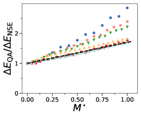
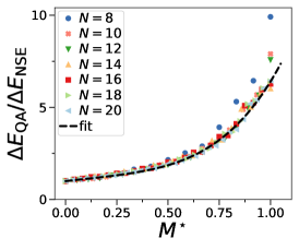
Here, we study the non-integrable Ising model with transverse and longitudinal fields combined with a discretized quantum annealing state as function of number of qubits . We vary the parameters of the Hamiltonian and the number of layers of the quantum annealing state. The initial state has an error , where is the energy of thequantum annealing state and the exact ground state. We plot the improvement of NSE in estimating the ground state. We find for all cases that collapses to a single curve for sufficient number of qubits when plotted against number of ansatz states divided by number of qubits . The result is shown in Fig.9. We find a collapse to a single curve for all cases for sufficiently large . We find that the NSE yields even better results when increasing the field of the Ising model or layers of the quantum annealing state. For , we find that the collapse becomes evident only for larger number of qubits compared to the other cases, which we suspect is due to quantum annealing providing worse estimates of the ground state energy when is small.
 (a)
(a)
 (b)
(b)
 (c)
(c)
 (d)
(d)
