Bayesian-Wilson coefficients in lattice QCD computations of valence PDFs and GPDs

Abstract

We propose an analysis method for the leading-twist operator product expansion based lattice QCD determinations of the valence parton distribution function (PDF). In the first step, we determine the confidence-intervals of the leading-twist ${\overline{\mathrm{MS}}}$ Wilson coefficients, $C_{n}(\mu^{2}z^{2})$, of the equal-time bilocal quark bilinear, given the lattice QCD matrix element of Ioffe-time distribution for a particular hadron H as well as the prior knowledge of the valence PDF, $f(x,\mu)$ of the hadron H determined via global fit from the experimental data. In the next step, we apply the numerically estimated $C_{n}$ in the lattice QCD determinations of the valence PDFs of other hadrons, and for the zero-skewness generalized parton distribution (GPD) of the same hadron H at non-zero momentum transfers. Our proposal still assumes the dominance of leading-twist terms, but it offers a pragmatic alternative to the usage of perturbative Wilson coefficients and their associated higher-loop uncertainties such as the effect of all-order logarithms at larger sub-Fermi quark-antiquark separations $z$.

I Introduction

The progress in determining the $x$-dependent hadron structures, such as the parton distribution functions (PDFs) and the generalized parton distribution functions (GPDs) Müller et al. (1994); Ji (1997); Radyushkin (1996) (for a review, see Diehl (2003)), has been quite rapid in the recent years, particularly owing to the perturbative matching frameworks such as the quasi-PDF Ji (2013, 2014), pseudo-PDF Radyushkin (2017); Orginos et al. (2017), current-current correlators Braun and Müller (2008) and the good lattice cross-sections approach Ma and Qiu (2018a, b). There are other ideas that are being used (for example, Martinelli and Sachrajda (1987); Liu and Dong (1994); Chambers et al. (2017); Detmold and Lin (2006); Detmold et al. (2021)), but we would restrict ourselves to the set of perturbative matching approaches for calculating PDFs in this paper. Roughly, the recurring idea in all the variants of the perturbative matching approaches is the factorization of certain equal-time boosted hadron matrix elements with a spatial operator separation $z$ (or the Fourier transform thereof into $x$-space) into a matching kernel and the structure functions, such as the PDF as a specific case. The usefulness of this factorization is that the matching kernel can be perturbatively evaluated and hence universal for all hadrons. We refer the reader to the recent reviews Constantinou (2021); Cichy and Constantinou (2019); Ji et al. (2020); Radyushkin (2020) on this broad topic for further details on the methodology and for the recent works in this direction.

Without any loss of generality, in this paper, we will specifically consider the case of equal-time multiplicatively renormalizable Ishikawa et al. (2017); Ji et al. (2018) correlator constructed from the quasi-PDF Ji (2013) matrix element

$$2E(P_{z}){\cal M}({\omega},z^{2})=\langle P_{z}|\bar{\psi}_{z}\gamma_{t}W_{z,0}\psi_{0}|P_{z}\rangle,$$ (1)

of quark and antiquark separated by a spatial distance $z$, also known as pseudo-Ioffe-time distribution Radyushkin (2017) (abbreviated as pseudo-ITD or just as ITD), and evaluated in an on-shell hadron with $P=(E,P_{z})$ moving with a spatial momentum $P_{z}$. The variable ${\omega}=zP_{z}$ is also known as the Ioffe-time Ioffe (1969); Braun et al. (1995). However, the rest of the paper can be equally carried over to any of the operators (e.g., Sufian et al. (2019, 2020)) under the umbrella of the good lattice cross-sections as well. The pertinent detail for this paper is that the the underlying factorization of ${\cal M}({\omega},z^{2})$, can be equivalently rewritten Braun and Müller (2008); Izubuchi et al. (2018) as a leading twist operator product expansion (OPE),

$${\cal M}({\omega},z^{2})=\sum_{n=0}C_{n}(z^{2}\mu^{2})\frac{(-i\omega)^{n}}{n!}\langle x^{n}\rangle(\mu)+{\cal O}(\Lambda_{\rm QCD}^{2}z^{2}),$$ (2)

valid up to higher-twist corrections, usually denoted as ${\cal O}(\Lambda_{\rm QCD}^{2}z^{2})$ terms. Occupying the central role in the above expression are the Wilson coefficients $C_{n}(z^{2}\mu^{2})$ that match the renormalized Euclidean matrix element in some scheme to the ${\overline{\mathrm{MS}}}$ PDF via the moments, and can be perturbatively computed at the hard scale set by $1/z$. In a typical lattice computation, the analytic form of $C_{n}$,

$$C_{n}(\mu^{2}z^{2})=\tilde{c}_{0}(n)+\tilde{c}_{1}(n)\ln(\mu^{2}z^{2})+\tilde{c}_{2}(n)\ln^{2}(\mu^{2}z^{2})+\ldots,$$ (3)

in terms of the coefficients $\tilde{c}$ of the powers of the singular logarithms $\ln(\mu^{2}z^{2})$, up to certain order in $\alpha_{s}$ is provided as an input, and in return, the PDF $f(x,\mu)$ and the Mellin moments, $\langle x^{n}\rangle=\int_{0}^{1}x^{n}f(x)dx$, are computed as outputs .

In the rest of the paper, we will consider the non-singlet, valence parton distribution functions. Unlike the singlet distributions, for the valence case, $xf(x)$ vanishes in the small-$x$ limit, and hence, enable us to neglect the associated systematic errors in the global fit determinations and in their first few Mellin moments. This lets us focus only on sources of uncertainty in the lattice computations of PDF. In the valence sector, the perturbative matching approach has been successfully applied to the lattice computations of PDF of the pion Sufian et al. (2019, 2020); Izubuchi et al. (2019); Gao et al. (2020); Lin et al. (2021) and the proton Joó et al. (2020, 2019a); Orginos et al. (2017); Bhat et al. (2021); Fan et al. (2020); Alexandrou et al. (2021a, 2018); Lin et al. (2020). In these calculations, the resulting reconstructed PDFs capture more or less the features of the phenomenologically determined PDFs (which we henceforth simply refer to as “pheno-PDFs”). By avoiding the issues of inversion problem to obtain $x$-dependent PDF, a direct comparison of the lattice ITD data itself with the corresponding expectation from the global analysis fits, obtained via perturbative matching, have only been qualitatively close enough (for example, Ref. Bhat et al. (2021) being one such comparison with NNPDF result Ball et al. (2017) for the proton at physical point, and Ref. Gao et al. (2020) for comparison of JAM18 result Barry et al. (2018) with 300 MeV pion). In particular, the deviation between the lattice ITD and the pheno-ITD increases with ${\omega}$ or $z$ as discussed in Sufian et al. (2021). These presumably point to the presence of yet uncontrolled systematic effect(s). Some of the reasons for this could be:

1. The effect of heavier than physical pion masses used in most of the calculations, but as we mentioned above, a recent computation Bhat et al. (2021) of the isovector nucleon PDF at the physical point still shows visible discrepancy with the ITD constructed from NNPDF global analysis Ball et al. (2017). The weak pion mass dependences seen in Joó et al. (2020); Sufian et al. (2020) in the range, $m_{\pi}\in[172,415]$ MeV, suggests this might not be the dominant contribution to the observed discrepancies even for computations at moderately heavier pion masses.

2. There could be lattice spacing corrections to pseudo-ITDs. For the case of pseudo-ITD renormalized in the ratio scheme, the lattice spacing effects were seen Gao et al. (2020) to mostly affect regions of ${\cal M}({\omega},z^{2})$ for $z={\cal O}(a)$. Such lattice spacing effect at small $z$ was also seen for the nucleon recently Karpie et al. (2021). Therefore, at least for renormalization methods like the ratio, the short-distance lattice spacing effects are less important and can be ignored provided one skips first few values of $z$. Hence, we do not consider this in this paper.

3. A more troublesome reason could be the presence of yet undetected large higher-twist contributions in the range of separations, $z\in[0.04,1]$ fm that are accessible in the computations today, but incorrectly taken as part of leading-twist contribution. However, a recent investigation Gao et al. (2020) of the higher-twist effect that dominate in the $P_{z}=0$ RI-MOM matrix element for the pion suggests that the higher-twist effect could be a minor, $\approx 40$ MeV effect that is atypically small compared to the QCD scale, $\Lambda_{\rm QCD}\approx 300$ MeV. By using ratio method (with ratio taken with respect to zero momentum as well as with non-zero momentum bare matrix element) for renormalization instead of the RI-MOM scheme Chen et al. (2018), it is reasonable to expect these leading $z^{2}$ higher-twist contributions to get approximately canceled leaving behind only a residual higher-twist contamination of the form $z^{2}{\omega}^{2}$ Karpie et al. (2018).

In this work, we take an optimistic stand on this matter and ask what if the remaining uncertainties in the leading-twist approach are predominantly unaccounted higher-loop corrections, and how to take care of our limited knowledge of the perturbative convergence of the Wilson coefficients in a probabilistic manner? This is the motivation for this paper.

There have been previous works to find ways to take into account the residual perturbative corrections and consider the question of whether the lattice results have perturbatively converged i.e., whether $C_{n}(z^{2})$ is perturbatively convergent at all potential values of $z$ that are used in a typical lattice analysis. There is an ongoing program to find higher loop corrections to $C_{n}$, with the state-of-the-art result at next-to-next-to-leading order (NNLO) published in Chen et al. (2020a, b); Li et al. (2021). In a recent paper Gao et al. (2021), the residual effect of higher-loops partially seen via resumming next-to-leading logarithms and threshold resummation was investigated in detail, wherein visible effects of resummation were seen in typical values of sub-fermi distances $z$. For the sake of argument, in addition to the resummation of lower-order logarithms, a priori it cannot be ruled out that the genuine higher-loop corrections and logarithmic terms that arise via 1PI diagrams could result in large numerical coefficients that multiply $\alpha_{s}^{m}$ factors, making the convergence of perturbation theory slower for the leading-twist approach. A method to take care of the renormalon ambiguity in the perturbation series was considered recently in Ji et al. (2021).

In this paper, we assume two things: first, that the lattice data for the matrix element has a leading-twist description. Second, we assume that the Wilson coefficients that enter the leading-twist OPE are hadron independent. Given these two assumptions, the idea we pursue in this paper is to replace a perturbatively determined $C_{n}$ with a probabilistically likely $C_{n}$ that is determined directly from the lattice matrix element data, and given a trustworthy knowledge of valence PDF of a hadron from global analysis of experimental input. The lattice determined $C_{n}$ can then be used in computing the PDFs of other hadrons, as well as to obtain the zero-skewness GPD. By turning the argument around, as this Bayesian approach is falsifiable, it would also be a good way to rule out the hypothesis of higher-loop corrections being important in matching the lattice calculations (which is the premise of this paper), or whether there are substantial higher-twist corrections affecting the lattice results. Therefore, at the cost of adding the systematics from the lattice computations for two different hadrons, the method presented in this paper will help disentangle the perturbative QCD systematics from systematics of nonperturbative lattice parton computations. One should note that our method is a novel way to make use of global analysis data in lattice computation, unlike the previous ways Bringewatt et al. (2021); Del Debbio et al. (2021); Cichy et al. (2019); Constantinou et al. (2020), where one tries to include the lattice data as one of the input to global analysis. In the rest of the paper, we explain the method and apply it to lattice mock-data, and some real published proton and pion lattice data.

II The method

In the traditional Bayesian reconstruction of PDFs $f(x)$ via fits (of parameters that characterize a certain PDF ansatz) to the lattice data for the matrix element ${\cal M}_{H}({\omega},z^{2})$ for a hadron $H$, one asks for the conditional probability distribution

$$P\bigg{(}f(x)\bigg{|}\mathrm{data\ for\ }{\cal M}_{H}\bigg{)}\propto P\bigg{(}\mathrm{data\ for\ }{\cal M}_{H}\bigg{|}f(x)\bigg{)}P\bigg{(}f(x)\bigg{)}.$$ (4)

One treats $P(\mathrm{data}|f)\sim e^{-\chi^{2}/2}$ via the $\chi^{2}$-minimization analysis to find the best fit value (i.e., the maximum a posteriori estimator) of $f(x)$ that maximizes the left-hand side probability, and its confidence interval. The assumption of a certain parametrization of the PDF is implicit in the prior $P(f)$. Methods based on the Bayesian reconstruction of PDFs so as to avoid the modeling bias in $f$ have been tried before Karpie et al. (2019). Instead of applying the Bayesian methods to the reconstruction of PDFs, in this work, we apply the same ideas to the determination of Wilson coefficients. We propose the following two-step scheme assuming one has lattice results for more than one hadron — results for ${\cal M}_{H}({\omega},z^{2})$ for a hadron $H$ (say, for the proton), and the lattice data for ${\cal M}_{H^{\prime}}({\omega},z^{2})$ for at least one additional hadron $H^{\prime}$ (say, for the pion).

II.1 Step-1: Fit the Wilson coefficients given the lattice data for a hadron and prior knowledge of its pheno-PDF

In the first step, we ask for the conditional probability distribution $Q$ for the set of $z$- and $n$-dependent Wilson-coefficients, $\{C_{n}\}=\left\{C_{n}(z)\text{\ for\ }z\in[a,z_{\rm max}]\text{\ and\ }n\in[0,N_{\rm max}]\right\}$, themselves, given the lattice data for the matrix element ${\cal M}_{H}({\omega},z^{2})$ for a hadron $H$, as well as the prior knowledge of the PDF $f_{H}(x)$ of the same hadron $H$ from phenomenological determinations,

$$Q(\{C_{n}\}) \equiv P\bigg{(}\{C_{n}\}\bigg{|}\mathrm{data\ for\ }{\cal M}_{H},f_{H}\bigg{)},$$ (5)

$$\propto P\bigg{(}\mathrm{data\ for\ }{\cal M}_{H}\bigg{|}\{C_{n}\};f_{H}\bigg{)}P\bigg{(}\{C_{n}\}\bigg{)}.$$ (7)

As is standard, the distribution $P(\mathrm{data\ for\ }{\cal M}_{H}|\{C_{n}\};f_{H})$ models the Gaussian fluctuation of the data around the theoretical model ${\cal M}^{\rm twist-2}({\omega},z;\{C_{n}\},f_{H})$. That is, we can conveniently define, $Q(\{C_{n}\})={\cal K}\exp(-\chi^{2}/2)$, with a normalizing constant ${\cal K}$ and

$$\chi^{2}\left(\{C_{n}\}\right)=\sum_{z,{\omega}}\frac{\left({\cal M}_{H}({\omega},z)-{\cal M}^{\rm twist-2}({\omega},z;\{C_{n}\},f_{H})\right)^{2}}{\sigma_{H}^{2}}\quad$$ (8)

$$\qquad\quad\quad\quad-2\ln\left(P(\{C_{n}\})\right),$$ (9)

where, $\sigma_{H}$ are the statistical errors associated with the lattice data for ${\cal M}_{H}({\omega},z)$. In our case, the theoretical model of the data is the twist-2 OPE that is dependent on the Wilson-coefficients as well the PDF (via its moments),

$${\cal M}^{\rm twist-2}({\omega},z;\{C_{n}\},f_{H})=\sum_{n=0}^{N_{\rm max}}C_{n}(z)\langle x^{n}\rangle_{H}\frac{(-i{\omega})^{n}}{n!},$$ (10)

with the Mellin moments, $\langle x^{n}\rangle_{H}=\int_{0}^{1}x^{n}f_{H}(x)dx$ as fixed numbers . Crucial to the Bayesian framework is the prior distribution $P(\{C_{n}\})$. For example, one could impose a non-informative prior on $C_{n}$, in which case $P(\{C_{n}\})$ is a constant for any choice of $\{C_{n}\}$, and therefore irrelevant. An alternative is to impose the degree of our confidence in the perturbative estimate (determined up to certain order), $C_{n}^{\rm pert}(z)$, through a Gaussian prior distribution,

$$-\ln\left(P(\{C_{n}\})\right)=\sum_{z,n}\left(\frac{\left(C_{n}(z)-C_{n}^{\rm pert}(z)\right)^{2}}{2\sigma_{\rm prior}^{2}}\right),$$ (11)

where the sum runs over all $z$-values and all the values of order $n$ in the twist-2 OPE that are included in the analysis. For example, one could use a broad prior width $\sigma_{\rm prior}$ to input no bias, or another choice could be two or three times the variations coming from changing the scale from $\mu/2$ to $2\mu$ used to determine $\alpha_{s}$ that enters $C_{n}^{\rm pert}(z)$.

This first step to characterize $Q(\{C_{n}\})$ can be implemented in different ways depending on the computational effort that one is willing to invest. In perhaps the most accurate implementation, one can simulate the multi-dimensional integral, ${\cal K}\int e^{-\frac{1}{2}\chi^{2}(\{C_{n}\})}{\cal D}C_{n}$, by using the Markov-Chain Monte Carlo (MCMC) numerical simulation. Thereby, one can estimate averages with respect to the distribution $Q$,

$$\left\langle F\right\rangle_{C_{n}}\equiv\int F(\{C_{n}\})Q(\{C_{n}\}){\cal D}C_{n},$$ (12)

of functions $F(\{C_{n}\})$ that depend on the Wilson coefficients. The Expected A Posteriori (EAP) values of $C_{n}$ obtained by using $F(\{C_{n}\})=\{C_{n}\}$ is one such example that can computed using MCMC. A cheaper alternative to using MCMC is to first summarize the information in $Q(\{C_{n}\})$ using the Maximum A Posteriori (MAP) values of $\{C_{n}\}$ that maximizes $Q(\{C_{n}\})$. That is

$$\{C_{n}^{\rm MAP}\}\equiv\underset{\{C_{n}\}}{\operatorname{arg}\,\operatorname{max}}\;Q(\{C_{n}\})=\underset{\{C_{n}\}}{\operatorname{arg}\,\operatorname{min}}\;\chi^{2}(\{C_{n}\}),$$ (13)

which can be obtained by the standard $\chi^{2}$-fits to the data by minimizing Eq. (9). The confidence intervals $C_{n}^{\rm MAP}\pm\sigma_{C_{n}}$ can be obtained by bootstrap. With the MAP values, a cheaper possibility to sample the distribution $Q$ is to approximate it parametrically by the multinormal distribution ${\cal N}\left(\{C_{n}^{\rm MAP},\sigma_{\rm C_{n}}\}\right)$. Instead of using a multinormal distribution, one could use the non-parametric bootstrap histogram of $\{C_{n}^{\rm MAP}\}$ obtained by performing the $\chi^{2}$ minimization in each of the bootstrap samples of the data. For demonstration purposes, we will use this simpler procedure in the latter half of paper. In these approximations to the true $Q(\{C_{n}\})$, it is important to resample the central values $C_{n}^{\rm pert}$ entering the prior distribution from $P(\{C_{n}\})$ in each bootstrap iteration, so as to ensure that in the absence of any constraint from the data, one reproduces the prior distribution $P(\{C_{n}\})$ rather converging to the same value in every iteration. For the sake of completion on the possible implementations of Step-1, as a crude approximation, one could simply ignore the uncertainty in $C_{n}^{\rm MAP}$ and use $Q(\{C_{n}\})\approx\delta(\{C_{n}\}-\{C_{n}^{\rm MAP}\})$ which will greatly simply the analysis steps above and those that follow. However, we do not follow this approximation here.

II.2 Step-2 : Determine the PDF of other hadrons with the computed Wilson coefficients

In the second step, we use the estimated $C_{n}$ from the first step to fit the ${\cal M}_{H^{\prime}}({\omega},z^{2})$-data for another hadron $H^{\prime}$. That is, we ask for the conditional probability on the parameters $\alpha$ describing the PDF $f_{H^{\prime}}(x;\alpha)$ of $H^{\prime}$ given the data and marginalized over the random choices of $\{C_{n}\}$ picked from the distribution $Q(\{C_{n}\})$,

$$P\bigg{(}f_{H^{\prime}}\bigg{|}\mathrm{data\ for\ }H^{\prime}\bigg{)}\propto$$ (14)

$$P(\alpha)\int P\bigg{(}\mathrm{data\ for\ }H^{\prime}\bigg{|}f_{H^{\prime}},\{C_{n}\}\bigg{)}Q(\{C_{n}\}){\cal D}C_{n}.$$ (15)

(16)

The distribution, $P(\alpha)$, on the right-hand side is the prior on the parameters $\alpha$ that enter $f_{H^{\prime}}$, given a fixed underlying model for the PDF. For example, $f_{H^{\prime}}(x;\alpha)$ could be the model $x^{a}(1-x)^{b}$, with $\alpha=\{a,b\}$. In the rest of the paper, we will consider a non-informative prior on $\alpha$, and hence, drop the prior term $P(\alpha)$ for the sake of simplicity. The distribution, $P\left(\mathrm{data\ for\ }H^{\prime}|f_{H^{\prime}},\{C_{n}\}\right)\equiv{\cal K}^{\prime}e^{-\chi^{\prime 2}(\alpha,\{C_{n}\})/2}$ with the normalizing constant ${\cal K}^{\prime}$, captures the Gaussian fluctuation of data for ${\cal M}_{H^{\prime}}$ around the twist-2 OPE theoretical model via

$$\chi^{\prime 2}\left(\alpha,\{C_{n}\}\right)=$$ (17)

$$\quad\sum_{z,{\omega}}\frac{\left({\cal M}_{H^{\prime}}({\omega},z)-{\cal M}^{\rm twist-2}({\omega},z;\{C_{n}\},\alpha)\right)^{2}}{\sigma_{H^{\prime}}^{2}}.$$ (18)

To be concrete, one is interested in a measure of the most probable value of $f_{H^{\prime}}$ and its confidence intervals. Similar to the discussion in Step-1, one such quantity that can be measured in an MCMC simulation is the EAP value of the PDF,

$$f_{H^{\prime}}^{\rm EAP}(x)={\cal K}^{\prime}\int f_{H^{\prime}}(x;\alpha)e^{-\frac{1}{2}\chi^{\prime 2}(\alpha,\{C_{n}\})}Q(\{C_{n}\}){\cal D}\alpha{\cal D}C_{n}.$$ (19)

To evaluate the above integral, one will sample the values of $\{C_{n}\}$ from the MCMC simulation as performed in Step-1 in order to capture the measure $Q(\{C_{n}\}){\cal D}C_{n}$, and perform a second MCMC simulation over the parameters $\alpha$. This would be computationally rather complex. Instead, as a simpler statistic for the probable value of $f_{H^{\prime}}(x;\alpha)$, one can find the Maximum Likelihood Estimate (MLE), $\left[f_{H^{\prime}}\right]^{\rm MLE}({C_{n}})$, that minimizes $\chi^{\prime 2}(\alpha,\{C_{n}\})$ for each instance of $\{C_{n}\}$ drawn from $Q(\{C_{n}\})$, and then perform an average over $C_{n}$. That is, one can use

$$f^{\rm avg}_{H^{\prime}}\equiv\left\langle\left[f_{H^{\prime}}\right]^{\rm MLE}\right\rangle_{C_{n}},$$ (20)

as an estimator of the PDF and its confidence intervals. To perform the average $\langle\ldots\rangle_{C_{n}}$, one needs to draw instances of $C_{n}$ sampled in Step-1. As mentioned previously, we will use the bootstrap sample of $\{C^{\rm MAP}_{n}\}$ from Step-1 as an approximation of $Q(\{C_{n}\})$ to perform the above step. To avoid extra symbols, we will simply use $f_{H^{\prime}}(x)$ to denote $f^{\rm avg}_{H^{\prime}}(x)$ and its error-bands in the rest of the paper.

The two steps could be done in such a way that collaboration-A does a dedicated computation of an ensemble of $\{C_{n}\}$ distributed according to $Q(\{C_{n}\})$ in its own set of gauge ensembles etc., using some hadron $H$, and collaboration-B takes this $Q(\{C_{n}\})$ as an input for its dedicated computation of $f_{H^{\prime}}(x)$ for hadron $H^{\prime}$. In this case, there is no correlation between a choice of $C_{n}^{\prime}$ and the re-sampled bootstrap configurations. In another way, a single lattice collaboration computes both pion and proton, preferably at the physical point and using the same set of configurations. In this case, one could reduce the statistical errors by sampling $Q(\{C_{n}\})$ so as to maintain correlations between the pion and proton data.

II.3 Remarks on the method

First, we have a choice as to which hadron we should consider first to determine the Wilson coefficients. If one has very accurate data, this question simply boils down to how well determined the pheno-PDFs of a given hadron is. For the unpolarized sector, using the proton valence PDF, which has been determined at NLO and NNLO level accuracy Ball et al. (2017) from the experimental data, as the known input would be the ideal choice. One can then input the set of $C_{n}$ from the proton analysis into the analysis of pion PDFs on the lattice. The downside to this order of steps is that the moments $\langle x^{n}\rangle$ of proton PDF approach zero faster as $n$ is increased, compared to the pion . Consequently, while one can determine $C_{n}(z)$ for to a higher order in $n$ (we expect about up to first three even $n$, as we will discuss later in the paper) using pion PDF as input, it would be difficult to do so using the proton. Nevertheless, this difficulty is purely statistics related and can be solved in a high-statistic study of the proton ITD in the future. On the other hand, the difficulty in using valence pion PDF as the input PDF is that unlike the proton PDF, the robustness of valence pion PDF from different analyses of experimental data Badier et al. (1983); Betev et al. (1985); Conway et al. (1989); Owens (1984); Sutton et al. (1992); Gluck et al. (1992, 1999); Wijesooriya et al. (2005); Aicher et al. (2010); Barry et al. (2018); Cao et al. (2021) are still being scrutinized. In this paper, to simply demonstrate the idea, we will use the pion PDF as the starting point, but use different versions of pheno-PDFs of pion as inputs in the lattice analysis, and then determine the $C_{n}$ for each such choice. In turn, this procedure will lead to different estimates of proton PDFs on the lattice. In this way, in addition to demonstrating the method, we would also be studying the impact of a good phenomenological determination of pion-PDF on the lattice determination of proton PDFs.

Secondly, let us elaborate on the method being a Bayesian extension of the traditional analysis of lattice PDFs. As our confidence in the perturbative Wilson coefficients increases, due to say its calculation up to a certain higher-order $m$, then by the Bayesian framework, one will choose the prior distribution that peaks more and more about the $m$-loop result for $\{C_{n}\}$. That is, one will choose $\sigma_{\rm prior}\to 0$ as the confidence is subsequently increased. In that case, the posterior distribution approaches a delta-function about the $m$-loop result, and one recovers back the usual way of analysis using a given perturbative $C_{n}$. This is the essence of the idea in this paper to treat our ignorance of $C_{n}$ in a probabilistic manner.

Thirdly, it is easy to see that the fitted coefficients will automatically satisfy the Altarelli-Parisi evolution to the same accuracy to which the input pheno-PDF moments satisfies the evolution, since the matrix element ${\cal M}_{H}$, that is renormalized in a lattice scheme such as the ratio, is independent of the factorization scale $\mu$. To expand on, the actual quantities that we obtain by fits are the $z$-dependent coefficients of the $(-i{\omega})^{n}/n!$-terms in the twist-2 OPE in Eq. (10). Let us call those coefficients $D_{n}(z)$. Since ${\cal M}_{H}$ has no knowledge of $\mu$, the coefficients $D_{n}(z)$ will be constants independent of $\mu$. By writing $D_{n}(z)=C_{n}(\mu,z)\langle x^{n}\rangle(\mu)$, it is clear that the $\mu$-dependence of fitted $C_{n}(\mu,z)$ will be the inverse $\mu$-dependence of $\langle x^{n}\rangle(\mu)$, which is dictated by the Altarelli-Parisi equation that the global fit PDF satisfies.

Fourthly, since we are using only the valence Mellin moments in the twist-2 OPE to determine $C_{n}$, it is not necessary to use the pheno-PDF values, and instead, one could use lattice determinations of Mellin moments obtained using the local twist-2 operators (e.g., Mondal et al. (2020); Alexandrou et al. (2021b) for recent studies). Using the local twist-2 operator approach, both even and odd Mellin moments can be computed. However, currently, only $\langle x^{2}\rangle$ even valence moment from such studies are usable as input to determine $C_{n}$ in the method we proposed (and only even $n$ enter the valence ITDs), and hence not a practical option currently.

III Generalization to zero-skewness GPD

Let us now consider the equal-time matrix element corresponding to the generalized parton distribution function (GPD) $f(x,t)$ at zero-skewness Liu et al. (2019a); Radyushkin (2019),

$$2E{\cal M}({\omega},z^{2},t=-q^{2})=\langle\vec{P}+\vec{q}/2|\bar{\psi}_{z}\gamma_{t}W_{z,0}\psi_{0}|\vec{P}-\vec{q}/2\rangle,$$ (21)

with spatial momentum $\vec{P}=(0,0,P_{z})$ and transverse momentum transfer $\vec{q}=(q_{x},q_{y},0)$, with $t=\vec{q}^{2}$. For this kinematics at zero skewness, $\xi=q_{z}/2P_{z}=0$, the corresponding leading twist OPE is given as Liu et al. (2019a); Radyushkin (2019) ,

$${\cal M}({\omega},z^{2},t)=\sum_{n=0}C_{n}(z^{2}\mu^{2})\frac{(-i{\omega})^{n}}{n!}\langle x^{n}\rangle(t,\mu),$$ (22)

with the same set of Wilson coefficients $\{C_{n}\}$ as in the case of forward PDF Liu et al. (2019a), but the GPD moments (i.e., the generalized form factors), $\langle x^{n}\rangle(t,\mu)$ being dependent on the momentum transfer $t$. Given this property of the $\xi=0$ GPD, it is straight forward to generalize the analysis scheme presented in the last section:

1. Determine $Q(\{C_{n}\})$ using the lattice forward matrix element data ${\cal M}_{H}({\omega},z^{2},t=0)$ of a hadron $H$ using the pheno-PDF $f_{H}(x)$ as a given. This step is the same as the step-1 described previously.

2. Using randomly sampled $\{C_{n}\}$ from the distribution $Q(\{C_{n}\})$, perform the analysis of zero skewness GPD of the same hadron $H$ at $t>0$ via $P\bigg{(}f_{H}(x,t)\bigg{|}\mathrm{data\ for\ }{\cal M}_{H}(t)\bigg{)}$ that is marginalized over $\{C_{n}\}$.

We expect this to be a less-noisy implementation as the GPD data of a hadron $H$ is expected to be correlated with the $t=0$ matrix element of the same hadron $H$ in a given ensemble. It would be interesting to see the data presented for valence pion GPD Chen et al. (2020c) and unpolarized proton GPD Alexandrou et al. (2020) analyzed in the manner suggested here.

In addition to the generalization to zero-skewness GPD, few other cases are also possible . The chiral-symmetry present in the massless quark limit ensures that the Wilson coefficients are the same for bilocal quark bilinear operators with $\gamma_{z}$ and $\gamma_{5}\gamma_{z}$ Dirac spinor structures Liu et al. (2020); Fan et al. (2020). That is, the matching factors are the same for the unpolarized PDF computed with $\gamma_{z}$ bilocal quark bilinear and the helicity PDF computed with $\gamma_{5}\gamma_{z}$ bilocal bilinear. Thus, the method presented here can be applied to the proton unpolarized PDF determined using $\gamma_{z}$ bilocal bilinear to determine the corresponding $\{C_{n}\}$, and then use them in the lattice computation of the proton helicity PDF. The drawback is that the $\gamma_{z}$ bilocal bilinear suffers from mixing with the scalar bilinear Constantinou and Panagopoulos (2017); Chen et al. (2018), adding to the systematics. In addition, the Wilson-coefficients for $\gamma_{z}$ bilocal bilinear also enters the leading-twist OPE that describes the Distribution Amplitude (DA) of the pion Braun and Müller (2008); Liu et al. (2019b); Radyushkin (2019).

IV Demonstration of the method using mock-data

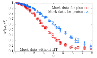
Figure 1: A mock-data for the real part of the pseudo-ITD for pion (red) and proton (blue) shown as a function of ${\omega}=zP_{z}$. The data from $z\in[a,12a]$ have been put together in the plot (and not distinguished by their $z$ values to avoid clutter), leading to visible corrections to the scaling with ${\omega}$ and will be captured by the Wilson coefficients $C_{n}(z)$. For parameters used to generate this data, refer text.

In this section, we apply the idea to a set of mock-data that we generated for the pion and proton pseudo-ITD ${\cal M}({\omega},z^{2})$, which are renormalized in the ratio scheme and set in a lattice with a spacing $a=0.06$ fm with an extent $L_{z}=48$ in the $z$-direction. Also, we will only be looking at the real part of the ITD, ${\rm Re}{\cal M}$, which corresponds to the nonsinglet valence contribution for both the proton and the pion. The point of using mock-data is that we exactly know what corrections to NLO matching we put in, and ask how this new framework will handle these corrections. We generated the mock-data for pseudo-ITD of $H$ (proton $p$ and pion $\pi$) by drawing sample means $\overline{{\cal M}}_{H}(zP_{z},z)$, for $z\in[a,12a]$ and $P_{z}aL_{z}/(2\pi)\in[1,5]$. The underlying distribution for the sample means $\overline{{\cal M}}_{H}$ (which one can think of as column vector of size 60 by linearizing ${\omega}$ and $z$) was the multinormal distributions, ${\cal N}\left(\overline{{\cal M}}^{0}_{H},\Sigma\right)$. The true central value $\overline{{\cal M}}^{0}_{H}$ of the multinormal distribution was engineered by hand so as to have corrections to NLO values of $C_{n}$, and certain amount of higher-twist correction, and written as

$$\overline{{\cal M}}^{0}_{H}({\omega},z^{2}) = \sum_{n=0}C^{\rm mock}_{n}(z^{2}\mu^{2})\frac{(-i{\omega})^{n}}{n!}\langle x^{n}\rangle_{H}$$ (24)

$$+\quad\left(e^{-\Lambda^{2}z^{2}{\omega}^{2}}-1\right),$$

where the moments $\langle x^{n}\rangle_{H}$ were inferred from the pheno-PDF values of $H$; namely, from the unpolarized NNPDF Ball et al. (2017) data at $\mu=3.2$ GeV for the proton, and the JAM20 Cao et al. (2021); Barry et al. (2018) data at $\mu=3.2$ GeV for the pion respectively. Since we are looking at the real part of the ITD, only the even $n$-values enter the above equation. We use a set of mock Wilson coefficients $C_{n}^{\rm mock}$ given by the coefficients of the $\ln^{j}(\mu^{2}z^{2})$ terms,

$$\tilde{c}_{n}(j)=\tilde{c}^{\rm NLO}_{n}(j)+\Delta\tilde{c}_{n}(j),\quad j=0,1,2,$$ (25)

used in Eq. (3). Above, $\tilde{c}^{\rm NLO}_{j}$ are the NLO values that can be read off from Izubuchi et al. (2018); Karpie et al. (2018), and $\Delta\tilde{c}_{j}$ are toy correction terms that we put in by hand to simulate the higher-loop corrections. Since we are working with ratio matrix elements, we simply take $C_{0}^{\rm mock}(\mu^{2}z^{2})=1$, as it is true to all orders. We added the residual higher-twist correction via the term in the second line of Eq. (24); it is motivated by its expansion as $\Lambda^{2}z^{2}{\omega}^{2}+\Lambda^{4}z^{4}{\omega}^{4}/2+\ldots$, which involves all $z^{k}$ type terms, and we have chosen it as a function of $z^{2}{\omega}^{2}$ as any leading $z^{2}{\omega}^{0}$ type higher-twist effect would most-likely have been canceled in the ratio scheme. As for the covariance matrix $\Sigma$ in the multinormal distribution, we made an ad hoc choice $\Sigma_{[z,{\omega}],[z^{\prime},{\omega}^{\prime}]}=\sigma_{z,{\omega}}\sigma_{z^{\prime},{\omega}^{\prime}}/(1+k|{\omega}-{\omega}^{\prime}|^{\delta})$, with the diagonal term being simply the $\sigma_{z,{\omega}}^{2}$ error term, and the $|{\omega}-{\omega}^{\prime}|^{\delta}$ term controlling how the correlation in the mock-data falls off as one moves along the off-diagonal elements; we chose $\delta=0.5$ and $k=0.5$ for maintaining some correlation in the mock-data. As for the diagonal error term, we chose a model $\sigma_{z,{\omega}}=r|{\omega}z|$ motivated by the fact that for a given value of $P_{z}$, the data gets noisier as $z$ increases, and that at a fixed $z$, the data at a higher $P_{z}$ is noisier. We used $r=0.0005$ for the pion and 0.0008 for the proton. The only justification for choosing all these models to generate mock-data is simply that it leads to reasonable looking data that is similar to what is seen in the published literature.

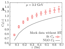
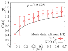
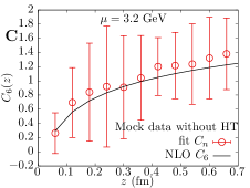
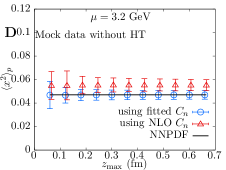
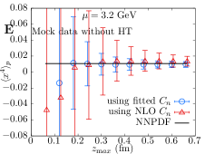
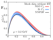
Figure 2: (Top panels A, B, C) The Wilson coefficients $C_{n}(z^{2})$ obtained from fits to the mock pion ITD are shown. The plots A, B, C are for $n=2,4,6$ respectively. The black curves are the respective NLO results for $C_{n}$. By construction of the mock-pion ITD, the underlying Wilson coefficients contain substantial corrections to the NLO $C_{n}$, and hence the observed discrepancy. (Bottom panels D, E) The Mellin moments, $\langle x^{2}\rangle$ and $\langle x^{4}\rangle$, extracted by twist-2 OPE fits to the proton pseudo-ITD over the range of $z\in[2a,z_{\rm max}]$ are shown as a function of range maximum $z_{\rm max}$ in the panels D and E respectively. The results using NLO $C_{n}(z^{2})$ as well as the $C_{n}(z^{2})$ obtained from fits to the pion ITD (shown in the top panels) are displayed together. The corresponding NNPDF moments that were used to produce mock-proton data are the black horizontal lines. In bottom panel F, the results from fits of the JAM-type two parameter ansatz $f(x)=x^{\alpha}(1-x)^{\beta}$ are shown using the two types of $C_{n}$.

IV.1 Case-1: When the dominant corrections are higher-loop corrections to leading-twist OPE

First, let us look at a case where there are only corrections to the NLO $C_{n}$, which we will denote as $C_{n}^{\rm NLO}$, via non-zero $\Delta\tilde{c}_{n}(j)$ terms, and no higher-twist correction terms, i.e., $\Lambda=0$ for both the pion and the proton. This is exactly the case where the our method has to work better than the one using finite order $C_{n}$, and therefore, it should not be surprising that we will account for the corrections at the end of this subsection. We experimented with different models of corrections to NLO Wilson coefficient (and the reader can try their own setup in the Jupyter notebook here git ), but we discuss an example case that we think is more plausible, with corrections given as $\left[\Delta\tilde{c}_{n}(0),\Delta\tilde{c}_{n}(1),\Delta\tilde{c}_{n}(2)\right]=\left[0.1037,0.0207,-0.0025\right]\ln(n+1)$. The choice of $\ln(n+1)$-dependence of the correction terms is inspired by the asymptotic behavior of the Harmonic functions that appear in the perturbative kernel and could be important to threshold resummation as discussed in Gao et al. (2021). The mock-data for ${\rm Re}{\cal M}$ that is generated from ${\cal N}\left(\overline{{\cal M}}^{0}_{H},\Sigma\right)$ for the proton and the pion are shown in Fig. 1.

By using the JAM20 Cao et al. (2021); Barry et al. (2018) determination of pion PDF as the fixed input, we fitted the coefficients $C_{n}(z)$ for even values of $n>0$ as the free parameters to the mock-pion data using the twist-2 expression in Eq. (10) with the truncation at $n=N_{\rm max}=10$. As discussed above, for the ratio pseudo-ITD, the value of $C_{0}(z)=1$, and hence it is not a fit parameter. The fits are analogous and non-parametric in $z$ to the type of fits used in “OPE without OPE” analysis Karpie et al. (2018) of moments as a function of $z$, with the modification being that we are now fitting the $z$-dependent coefficients $C_{n}(z)$ instead of moments. We imposed a prior on $C_{n}$ from $C^{\rm NLO}_{n}$ with a rather broad width of $\sigma_{\rm prior}$ of 100% of $C^{\rm NLO}_{n}$ at any $z$. In the top panels A, B and C of Fig. 2, we show the three of the fitted $C_{n}(z)$ for $n=2,4$ and 6 as a function of $z$. These central (MAP) values and their errors shown in the plot (and the covariances between different $C_{n}(z)$ which are not shown) summarize the abstract posterior distribution $Q(\{C_{n}\})$ we used in our discussion of the method. For comparison, $C^{\rm NLO}_{n}$ is also shown as the black curve, which clearly disagrees with the fitted $C_{n}$, especially for $C_{2}$. This is expected by construction in this example mock-data. For $z/a=1$ for $C_{4}$ and $z/a\leq 4$ for $C_{6}$, the fitted values fall exactly on the NLO curve. This is due to the prior imposed, as there is no information on $C_{n}$ for these $z$ and its knowledge is purely derived from the prior. As $z$ is increased, one sees a cross-over from a prior-driven fit to a more data-driven one.

In the second step, we used the $C_{n}$ obtained above in the twist-2 OPE analysis of the mock proton pseudo-ITD data shown in Fig. 1. We performed a variant of the “OPE without OPE” analysis, in which we fitted proton moments $\langle x^{2}\rangle_{p},\langle x^{4}\rangle_{p}$ and $\langle x^{6}\rangle_{p}$ as free fit parameters in the twist-2 OPE expression, to the proton mock-data satisfying, $z\in[2a,z_{\rm max}]$ and all momenta. We took care of the uncertainty in $C_{n}$ by randomly drawing from the bootstrap samples obtained in the analysis of the pion in the first step. We repeated these fits by increasing $z_{\rm max}$ gradually. We have shown the dependence of the fitted moments $\langle x^{2}\rangle_{p}$ and $\langle x^{4}\rangle_{p}$ on $z_{\rm max}$ in the bottom panels D and E of Fig. 2, respectively. As expected, $\langle x^{2}\rangle_{p}$ from the fits using $C_{n}$ obtained from the pion agrees with the NNPDF value, which is the underlying PDF used to generate the proton pseudo-ITD mock-data. Similar to the case in actual lattice computations presently, the signal for $\langle x^{4}\rangle_{p}$ is poor at shorter $z_{\rm max}$, and albeit up to errors, the results with fitted $C_{n}$ agrees better with NNPDF value than the NLO $C_{n}$ as we venture to larger $z_{\rm max}$. In the bottom panel F of Fig. 2, we demonstrate how this method can also be applied in the reconstruction of $x$-dependent PDF by using a two-parameter ansatz of the form, $f(x)\sim x^{\alpha}(1-x)^{\beta}$; for this fit, one simply writes the moments as a function of $\alpha$ and $\beta$, and then performs the fits using the twist-2 OPE formula in Eq. (10) with $\{C_{n}\}$ being from either NLO or from the fits to the pion. The PDF reconstruction analysis with fitted $C_{n}$ reproduces the proton PDF, $f_{p}(x)$ to a better accuracy, whereas the one using the NLO kernel does not, as expected in this example. Through the above analysis of the mock-data, we have elaborated the typical steps we expect to be involved in the implementation of the method.

IV.2 Case-2: Possibility of suppressing higher-twist effects

The method we have laid out still assumes that the leading twist OPE describes the lattice data to a good accuracy. However, given that we only know the data up to errors, we can ask if the higher twist corrections can effectively be absorbed into effective Wilson coefficients determined by fits; we have to admit that this procedure is not pristine. In order to look for this possibility, let us consider a higher-twist correction to Eq. (10) of the form $\Lambda_{\pi}^{2}z^{2}{\omega}^{2}$ for the pion pseudo-ITD and $\Lambda_{p}^{2}z^{2}{\omega}^{2}$ for the proton pseudo-ITD. Let us first assume that such a higher-twist effect is more or less hadron mass independent, and that $\Lambda_{\pi}\approx\Lambda_{p}=\Lambda$. In the first step, when we do the fits of $\{C_{n}\}$ to, say the pion, such a higher-twist term can effectively be absorbed into a Wilson-coefficient given by

$$C_{2}^{\rm eff}(z)\equiv C_{2}^{\rm twist-2}(\mu^{2}z^{2})-\frac{2\Lambda^{2}z^{2}}{\langle x^{2}\rangle_{\pi}},$$ (26)

where $C_{2}^{\rm twist-2}(\mu^{2}z^{2})$ is the part of the fitted value that is the actual twist-2 Wilson coefficient. When such an effective $C_{2}^{\rm eff}(z)$ is used in the analysis of the proton pseudo-ITD, the net higher-twist correction in proton gets reduced to $\Lambda^{2}\left(1-\frac{\langle x^{2}\rangle_{p}}{\langle x^{2}\rangle_{\pi}}\right)z^{2}{\omega}^{2}$, which by putting in values for the moments at $\mu=3.2$ GeV, can be estimates to be a 70% reduction. On the other hand, if the higher-twist correction term $\Lambda_{p},\Lambda_{\pi}$ were proportional to the proton and pion masses respectively, there would hardly be any reduction in higher-twist term for the proton by this process. Unfortunately, the property of the higher-twist correction in the lattice data are unknown.

We repeated the mock-data analysis presented in the previous sub-section, but this time, included the same value of $\Lambda\neq 0$ in Eq. (24) for both the pion and the proton. We used a value of $\Lambda\approx 30$ MeV, which was found in the pseudo-ITD in RI-MOM scheme Gao et al. (2020), and even smaller in the ratio scheme. We performed the analysis in the similar way as described in the previous subsection by inputting the JAM20 pion-PDF to determine $C_{n}$ (which are effective now due to non-zero $\Lambda$). We show the result of the reconstructed proton PDF in Fig. 3. The use of fitted $C_{n}$ brings the estimated PDF closer to the actual proton PDF underlying the data when compared to the result obtained by using the NLO $C_{n}$. But, the results still disagree with the NNPDF curve due to the fact that the higher-twist corrections are canceled only partially.

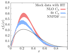
Figure 3: The result of $x$-dependent PDF fit to the proton mock-data containing higher-twist (HT) correction (see text) using a two parameter ansatz $f(x)=x^{\alpha}(1-x)^{\beta}$. The results using NLO $C_{n}$ and using an effective $C_{n}$ from fits to the mock-data for the pion are shown. The actual underlying PDF (NNPDF) that is used to produce the mock-proton data is shown by the black curve.

V Application to some selected published results

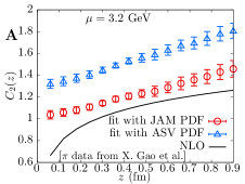
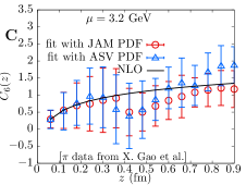
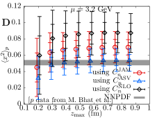
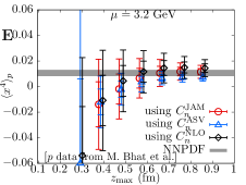
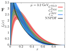
Figure 4: Top panels A, B, C show $C_{n}(z)$ as a function of $z$ obtained by fits to the pion reduced ITD data taken from a previously published result in X. Gao et al Gao et al. (2020). The fits were made using two different pheno-PDFs at $\mu=3.2$ GeV, namely, using the JAM20 PDF (red) and the ASV soft-gluon resummed estimate (blue). The NLO results for $C_{n}$ are the black curves. Bottom panels D, E, F show the application of $C_{n}$ extracted from the pion, to the analysis of the proton pseudo-ITD data presented in M. Bhat et al Bhat et al. (2021). The panels D, E show the fitted values of $\langle x^{2}\rangle_{p}$ and $\langle x^{4}\rangle_{p}$ as function of the maximum value of $z=z_{\rm max}$ of the fit range $z\in[2a,z_{\rm max}]$. The red, blue and the black points correspond to the estimates using the values of $C_{n}$ obtained using JAM20 pion PDF, using ASV PDF and the NLO values respectively. The estimate of the moments from the NNPDF at $\mu=3.2$ GeV are shown as horizontal black bands. The panel F show the proton PDFs reconstructed using two-parameter ansatz using the three-types of $C_{n}$.

In the last part of the paper, we apply our methodology to some of the previously published lattice results from different collaborations. However, we should remark that our analysis is certainly crude as we simply take the central values and errors presented in the publications, and we do not take into account the correlated statistical fluctuations in the data. More importantly, we will apply this method to some cases where the computations were performed with heavier than physical pion masses. We believe this is not a serious issue, at least for the pion PDF (c.f., Detmold et al. (2003); Sufian et al. (2020)). However, looking forward to the future, where more computations of both the pion and proton at the physical point might be forthcoming, we expect this method will be more appropriate. However, with these cautions, let us apply the method to some of the existing data in the literature.

The details of the published lattice QCD results for the pion and proton that we borrow the data (central-value and error) from, are as follows. For the pion, we take the ratio pseudo-ITD results Gao et al. (2020) for a 300 MeV pion determined on an ensemble with $a=0.06$ fm and lattice size of $48^{3}\times 64$. For the proton, we take the ratio ITD results at the physical point Bhat et al. (2021) obtained on an ensemble with $a=0.0938$ fm on $48^{3}\times 96$ lattices. For complete details on the lattice methods used in these studies, we refer the reader to the respective papers Gao et al. (2020); Bhat et al. (2021).

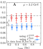
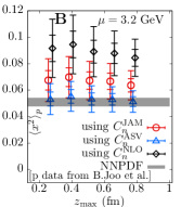
Figure 5: Panel A: Wilson coefficients $C_{n}^{\rm JAM}$ and $C_{n}^{\rm ASV}$ obtained from fit to pion pseudo-ITD data (taken from X. Gao et.al Gao et al. (2020) and shown in the top panels of Fig. 4) are applied to a completely different pion pseudo-ITD result taken from B. Joó et al. Joó et al. (2019b) to check for internal consistency and weak dependence on mass and lattice spacing. The result of two sets (red and blue) of fitted moments $\langle x^{2}\rangle_{\pi}$ obtained from the usage of $C_{n}^{\rm JAM}$ and $C_{n}^{\rm ASV}$ are shown as a function of fit range $z\in[2a,z_{\rm max}]$. For comparison, $\langle x^{2}\rangle_{\pi}$ from JAM20 and ASV are shown as dot-dashed and dashed lines. Panel B: A similar analysis of proton moment $\langle x^{2}\rangle_{p}$ using $C_{n}^{\rm JAM},C_{n}^{\rm ASV},C_{n}^{\rm NLO}$ as applied to the proton data obtained in B. Joó et al. Joó et al. (2019a) in the same ensemble as Joó et al. (2019b), and shown as a function of $z_{\rm max}$. The NNPDF result is shown for comparison.

We followed the same set of steps as described for the analysis of mock-data sets for these real lattice data, and hence we will keep the details brief. We used the pion PDF as the starting point. However, in the analysis here, in addition to the JAM20 pion PDF, we also included the ASV pion PDF estimate Aicher et al. (2010) (obtained by a reanalysis of the Fermilab data Conway et al. (1989) by including soft-gluon resummation). In the pion PDF literature, there is still an ongoing debate on whether the large-$x$ exponent $\beta$ is closer to 1 or about 2 Nguyen et al. (2011); Chen et al. (2016); Bednar et al. (2020); Aicher et al. (2010); Ruiz Arriola (2002); Broniowski and Ruiz Arriola (2017); de Teramond et al. (2018); Ding et al. (2020). In the top panels (A, B and C) of Fig. 4, we show the Wilson coefficients $C_{2}$, $C_{4}$ and $C_{6}$ obtained by fits to the pion pseudo-ITD data. The fitted values of $C_{n}$ obtained by assuming the JAM20 PDF as the input PDF, are shown as red circles in the plots. On the other hand, when we assumed that the ASV pion PDF at the same $\mu=3.2$ GeV scale as the given input PDF, we obtained the points shown in blue. For brevity, we will refer to the two sets of Wilson coefficients as $C_{n}^{\rm JAM}$ and $C_{n}^{\rm ASV}$, respectively. We remark that it would be a good idea to skip the first one or two lattice points for $C_{2}$ in the above plots as they are likely to be affected by small-$z$ lattice artifacts. To compare, the NLO values of $C_{n}$ are shown as the black curves, which lie comparatively closer to $C^{\rm JAM}_{n}$ than to $C^{\rm ASV}_{n}$. To rephrase, if one is confident that the ASV result is the correct pion PDF, then it implies that even the first non-trivial Wilson coefficient $C_{2}$ needs to have about 40% corrections to NLO $C_{2}$ resulting from higher-loop terms (given the assumption that higher-twist terms are not as important). For $C_{2}$ and $C_{4}$, the fits are driven by the lattice data as well as the input PDF for all $z$, whereas for $C_{6}$, the data is driven only by NLO prior for $z<0.3$ fm and then there is cross-over to data-driven regime for larger $z$.

In the next step, we applied $C^{\rm JAM}_{n}$ and $C^{\rm ASV}_{n}$ determined above to the proton pseudo-ITD lattice data. We dealt with the mismatch of lattice spacing between the two lattice calculations by interpolation. We first fitted the even moments, $\langle x^{2}\rangle_{p}$ and $\langle x^{4}\rangle_{p}$ to the proton pseudo-ITD data using twist-2 OPE truncated at ${\cal O}({\omega}^{4})$ containing the choices of Wilson coefficients as $C^{\rm JAM}_{n},C^{\rm ASV}_{n}$ and $C^{\rm NLO}_{n}$ at $\mu=3.2$ GeV. We performed these fits including the data with $z\in[2a,z_{\rm max}]$ for $z_{\rm max}$ up to 0.75 fm. The results for $\langle x^{2}\rangle_{p}$ and $\langle x^{4}\rangle_{p}$ from these fits are shown as a function of the maximum of the fit range, $z_{\rm max}$, in the panels D and E of Fig. 4. The black, blue and red points are the results from such fits using $C_{n}^{\rm NLO},C_{n}^{\rm ASV},C_{n}^{\rm JAM}$ respectively. For comparison, the black bands are NNPDF estimates of the proton moments at $\mu=3.2$ GeV. For $z_{\rm max}\approx 0.24$ fm, there is a discernible signal for $\langle x^{2}\rangle_{p}$, while $\langle x^{4}\rangle_{p}$ remains comparatively noisier. To account for the possibility of an underestimation of the errors in our analysis due to the absence of any correlated statistical fluctuations, we conservatively included both the 1-$\sigma$ as well as the 2-$\sigma$ errors in the plots for the moments. The NLO result for $\langle x^{2}\rangle_{p}$ is a bit higher than the NNPDF value (as also observed in the actual full-fledged analysis in Bhat et al. (2021)). The usage of $C_{n}^{\rm JAM}$ leads to a slight decrease in the estimated value of $\langle x^{2}\rangle_{p}$, and surprisingly, the largest change comes from the usage of $C_{n}^{\rm ASV}$, which lowers the estimated $\langle x^{2}\rangle_{p}$ that also agrees better with the NNPDF value. For $\langle x^{4}\rangle_{p}$, there are corresponding changes in the central values depending which $C_{n}$ is used, but completely masked by the larger error-bars. In the bottom panel-F, we show the unpolarized proton PDF, $f_{p}(x)$, that we reconstructed using a simple, $f_{p}(x)\sim x^{\alpha}(1-x)^{\beta}$ ansatz. Again, the results obtained using the three types of $C_{n}$ are shown in the different colors; the 2-$\sigma$ estimate is the outer-band and 1-$\sigma$ result is the inner-band enclosed by the solid lines. The $x$-dependent results are sensitive to which Wilson coefficient is used, and particularly, the result obtained using $C_{n}^{\rm ASV}$ agrees better with the NNPDF curve.

In order to see if the results presented above are some artifacts of putting together the results from two completely different lattice calculations, at different pion masses (with only the proton at physical point) and at different lattice spacings, we repeated the above analysis to the central-value and error data of the pion and proton pseudo-ITDs that we borrowed from the papers Joó et al. (2019b, a) by the HadStruc collaboration. The results reported in these papers used $32^{3}\times 96$ lattice with $a=0.127$ fm at a heavier pion mass of 415 MeV. The analysis of the 415 MeV pion data from Ref. Joó et al. (2019b) by applying the set of $C_{n}$ obtained also from the pion, with a 300 MeV mass and from a completely different data in Gao et al. (2020), is an interesting exercise. If there is not much lattice spacing and pion mass dependence in the two pion data, then the analysis using $C_{n}^{\rm JAM}$ from panels-(A,B,C) in Fig. 4 should result in the JAM20 moments as it is the initial input PDF in this case, and similarly, an analysis using $C_{n}^{\rm ASV}$ should result in ASV moments. In the panel-A of Fig. 5, we show $\langle x^{2}\rangle_{\pi}$ from such an analysis by fitting the moments over a range $z\in[2a,z_{\rm max}]$. We have again conservatively plotted both the 1-$\sigma$ and the 2-$\sigma$ errors. It is satisfying that this pion analysis reproduces the JAM20 and ASV moments as per our initial expectation. In the right panel-B of Fig. 5, we similarly show the result of applying $C_{n}^{\rm JAM},C_{n}^{\rm ASV}$ and $C_{n}^{\rm NLO}$ to the proton data from Joó et al. (2019a). The result is very similar to the one we observed in the panels-(D,E) of Fig. 4, with a similar effect of the choice of $C_{n}$ on the determined moments.

Given the cautions we offered at the beginning of this section, we need to be careful about the conclusions we can draw from the observations we have made. First, one should pay attention to fact that the usage of ASV versus JAM20 pion PDF as input PDFs leads to changes in $C_{n}(z)$ even for $n$ as small as 2. To contrast, in Ref. Gao et al. (2021), the corresponding threshold resummation for the pseudo-ITD calculation was investigated as the effect of potentially large $\alpha_{s}\ln(n)$ and $\alpha_{s}\ln^{2}(n)$ terms that will be present in $C_{n}$ at larger $n$, and thus will not affect the smaller $n$. Thus it is paradoxical that imposing the correctness of ASV PDF automatically implies a big correction to $C_{n}$ even for small $n$; we do not have a resolution in this paper. Thus, it would be important to repeat the exercise presented in this section to the lattice data for pion pseudo-ITD at the physical point when available in the future to see if the observation we have made still stands. Secondly, we see that an unaccounted larger higher-loop correction to $C_{n}$ starting from $n=2$ is sufficient for a better agreement between lattice computations of proton PDF and the phenomenological estimates, without any necessity to invoke higher-twist contaminations to the leading-twist OPE. The curious agreement of the lattice estimation for the proton moments and the PDF when $C_{n}^{\rm ASV}$ is used in the analysis instead of NLO $C_{n}$, brings forward the great impact a better determination of the pion PDF from global analysis in the future (c.f., Aguilar et al. (2019); Adams et al. (2018)) will have on a lattice computations of proton PDFs; a somewhat unexpected and interesting connection due to the method presented here.

VI Discussion

The method we advocated in this paper for lattice determination of valence PDFs consists of the following steps: (1) The leading-twist Wilson coefficients $C_{n}(\mu z)$ are determined directly by fitting the lattice data for a hadron, say the pion, by assuming the pion PDF is known well from phenomenological determinations and then taken as an input for the lattice analysis. At this step, our degree of confidence that a perturbative calculation at a given order is sufficient can be incorporated via addition of priors to the fits. (2) The $C_{n}(z)$ obtained from fits is then used in the analysis of lattice data to determine the PDF of another hadron, say, the proton by performing the usual reconstruction analysis methods to determine the $x$-dependent PDF, except that one replaces the perturbative matching coefficients with the one obtained from the pion, in this example. (3) One can also use the fitted values of $C_{n}$ in the analysis of zero-skewness GPD of, say the pion itself, at non-zero momentum transfers. We demonstrated the feasibility of this method by applying it to a set of mock-data, as well as to some published lattice pseudo-ITD data for the pion (at 300 MeV and 415 MeV) and the proton (at physical point and at 415 MeV). In doing so, we showed how the precise extraction of pion-PDF from the experimental data can have an impact on lattice studies of proton PDF, indirectly via the method we presented.

A drawback of the method is that there should be a good determination of pheno-PDF; this is achievable for the valence unpolarized PDF, but fails for the nonsinglet helicity and transversity PDFs since they are defined only for the proton. In such cases, the analysis strategy (3) is still viable, i.e., extend to zero-skewness helicity and transversity GPD of proton by inputting the experimental values of helicity and transversity PDF of proton respectively. This can also be tested in the helicity GPD data already presented in Alexandrou et al. (2020). In the future, it would also be interesting to extend this study to the iso-singlet PDF cases wherein the small-$x$ uncertainties in the global fit PDF themselves might need to be propagated into the analysis of lattice matrix elements (for example, see Ref. Ball et al. (2018) for a discussion of uncertainties from small-$x$ logarithms in global fit determination of singlet PDFs).

One could ask why should one perform this rather complicated procedure when one is, say, 75% certain that the correction to the Wilson coefficient $C_{2}(z)$ from higher-loop calculation will be less than 2%. In fact, the point of the paper was to generalize the perturbative matching method in such a way as to fold in our uncertainties about perturbative Wilson coefficients itself in the analysis; the Bayesian approach achieves this for us. In the example, we would arrange the Bayesian prior distribution of $C_{2}(z)$ in such a way that it is 75% likely that the $C_{2}$ lies within $2\%$ of the NLO Wilson coefficient. This way, we are making the degree of our ignorance of $C_{n}$ quantitative.

A reasonable concern could be that the experimental data is known only up to NLO or NNLO order, and hence, why should one use a procedure other than using NLO or NNLO value of $C_{n}$ for matching. The assumption we are implicitly making here is that the perturbative convergence of pheno-PDFs is fast and well-understood, whereas it does not necessarily guarantee a rapidly converging perturbative Wilson coefficients that are used to match PDFs to the lattice matrix elements. Thus, the solution, which in retrospect appears very simple, is to replace the two different perturbative calculations (one to extract pheno-PDF and the other to match lattice results), with a single well-studied perturbative step that has been used to determine the pheno-PDF via global analysis.

References

- Müller et al. (1994) D. Müller, D. Robaschik, B. Geyer, F. M. Dittes, and J. Hořejši, Fortsch. Phys. 42, 101 (1994), arXiv:hep-ph/9812448 .
- Ji (1997) X.-D. Ji, Phys. Rev. Lett. 78, 610 (1997), arXiv:hep-ph/9603249 .
- Radyushkin (1996) A. V. Radyushkin, Phys. Lett. B 380, 417 (1996), arXiv:hep-ph/9604317 .
- Diehl (2003) M. Diehl, Phys. Rept. 388, 41 (2003), arXiv:hep-ph/0307382 .
- Ji (2013) X. Ji, Phys. Rev. Lett. 110, 262002 (2013), arXiv:1305.1539 [hep-ph] .
- Ji (2014) X. Ji, Sci. China Phys. Mech. Astron. 57, 1407 (2014), arXiv:1404.6680 [hep-ph] .
- Radyushkin (2017) A. V. Radyushkin, Phys. Rev. D 96, 034025 (2017), arXiv:1705.01488 [hep-ph] .
- Orginos et al. (2017) K. Orginos, A. Radyushkin, J. Karpie, and S. Zafeiropoulos, Phys. Rev. D 96, 094503 (2017), arXiv:1706.05373 [hep-ph] .
- Braun and Müller (2008) V. Braun and D. Müller, Eur. Phys. J. C 55, 349 (2008), arXiv:0709.1348 [hep-ph] .
- Ma and Qiu (2018a) Y.-Q. Ma and J.-W. Qiu, Phys. Rev. D 98, 074021 (2018a), arXiv:1404.6860 [hep-ph] .
- Ma and Qiu (2018b) Y.-Q. Ma and J.-W. Qiu, Phys. Rev. Lett. 120, 022003 (2018b), arXiv:1709.03018 [hep-ph] .
- Martinelli and Sachrajda (1987) G. Martinelli and C. T. Sachrajda, Phys. Lett. B 196, 184 (1987).
- Liu and Dong (1994) K.-F. Liu and S.-J. Dong, Phys. Rev. Lett. 72, 1790 (1994), arXiv:hep-ph/9306299 .
- Chambers et al. (2017) A. J. Chambers, R. Horsley, Y. Nakamura, H. Perlt, P. E. L. Rakow, G. Schierholz, A. Schiller, K. Somfleth, R. D. Young, and J. M. Zanotti, Phys. Rev. Lett. 118, 242001 (2017), arXiv:1703.01153 [hep-lat] .
- Detmold and Lin (2006) W. Detmold and C. J. D. Lin, Phys. Rev. D 73, 014501 (2006), arXiv:hep-lat/0507007 .
- Detmold et al. (2021) W. Detmold, A. V. Grebe, I. Kanamori, C. J. D. Lin, R. J. Perry, and Y. Zhao, (2021), arXiv:2103.09529 [hep-lat] .
- Constantinou (2021) M. Constantinou, Eur. Phys. J. A 57, 77 (2021), arXiv:2010.02445 [hep-lat] .
- Cichy and Constantinou (2019) K. Cichy and M. Constantinou, Adv. High Energy Phys. 2019, 3036904 (2019), arXiv:1811.07248 [hep-lat] .
- Ji et al. (2020) X. Ji, Y. Liu, Y.-S. Liu, J.-H. Zhang, and Y. Zhao, (2020), arXiv:2004.03543 [hep-ph] .
- Radyushkin (2020) A. V. Radyushkin, Int. J. Mod. Phys. A 35, 2030002 (2020), arXiv:1912.04244 [hep-ph] .
- Ishikawa et al. (2017) T. Ishikawa, Y.-Q. Ma, J.-W. Qiu, and S. Yoshida, Phys. Rev. D 96, 094019 (2017), arXiv:1707.03107 [hep-ph] .
- Ji et al. (2018) X. Ji, J.-H. Zhang, and Y. Zhao, Phys. Rev. Lett. 120, 112001 (2018), arXiv:1706.08962 [hep-ph] .
- Ioffe (1969) B. L. Ioffe, Phys. Lett. B 30, 123 (1969).
- Braun et al. (1995) V. Braun, P. Gornicki, and L. Mankiewicz, Phys. Rev. D 51, 6036 (1995), arXiv:hep-ph/9410318 .
- Sufian et al. (2019) R. S. Sufian, J. Karpie, C. Egerer, K. Orginos, J.-W. Qiu, and D. G. Richards, Phys. Rev. D 99, 074507 (2019), arXiv:1901.03921 [hep-lat] .
- Sufian et al. (2020) R. S. Sufian, C. Egerer, J. Karpie, R. G. Edwards, B. Joó, Y.-Q. Ma, K. Orginos, J.-W. Qiu, and D. G. Richards, Phys. Rev. D 102, 054508 (2020), arXiv:2001.04960 [hep-lat] .
- Izubuchi et al. (2018) T. Izubuchi, X. Ji, L. Jin, I. W. Stewart, and Y. Zhao, Phys. Rev. D 98, 056004 (2018), arXiv:1801.03917 [hep-ph] .
- Lin et al. (2018) H.-W. Lin et al., Prog. Part. Nucl. Phys. 100, 107 (2018), arXiv:1711.07916 [hep-ph] .
- Izubuchi et al. (2019) T. Izubuchi, L. Jin, C. Kallidonis, N. Karthik, S. Mukherjee, P. Petreczky, C. Shugert, and S. Syritsyn, Phys. Rev. D 100, 034516 (2019), arXiv:1905.06349 [hep-lat] .
- Gao et al. (2020) X. Gao, L. Jin, C. Kallidonis, N. Karthik, S. Mukherjee, P. Petreczky, C. Shugert, S. Syritsyn, and Y. Zhao, Phys. Rev. D 102, 094513 (2020), arXiv:2007.06590 [hep-lat] .
- Lin et al. (2021) H.-W. Lin, J.-W. Chen, Z. Fan, J.-H. Zhang, and R. Zhang, Phys. Rev. D 103, 014516 (2021), arXiv:2003.14128 [hep-lat] .
- Joó et al. (2020) B. Joó, J. Karpie, K. Orginos, A. V. Radyushkin, D. G. Richards, and S. Zafeiropoulos, Phys. Rev. Lett. 125, 232003 (2020), arXiv:2004.01687 [hep-lat] .
- Joó et al. (2019a) B. Joó, J. Karpie, K. Orginos, A. Radyushkin, D. Richards, and S. Zafeiropoulos, JHEP 12, 081 (2019a), arXiv:1908.09771 [hep-lat] .
- Bhat et al. (2021) M. Bhat, K. Cichy, M. Constantinou, and A. Scapellato, Phys. Rev. D 103, 034510 (2021), arXiv:2005.02102 [hep-lat] .
- Fan et al. (2020) Z. Fan, X. Gao, R. Li, H.-W. Lin, N. Karthik, S. Mukherjee, P. Petreczky, S. Syritsyn, Y.-B. Yang, and R. Zhang, Phys. Rev. D 102, 074504 (2020), arXiv:2005.12015 [hep-lat] .
- Alexandrou et al. (2021a) C. Alexandrou, K. Cichy, M. Constantinou, J. R. Green, K. Hadjiyiannakou, K. Jansen, F. Manigrasso, A. Scapellato, and F. Steffens, Phys. Rev. D 103, 094512 (2021a), arXiv:2011.00964 [hep-lat] .
- Alexandrou et al. (2018) C. Alexandrou, K. Cichy, M. Constantinou, K. Jansen, A. Scapellato, and F. Steffens, Phys. Rev. Lett. 121, 112001 (2018), arXiv:1803.02685 [hep-lat] .
- Lin et al. (2020) H.-W. Lin, J.-W. Chen, and R. Zhang, (2020), arXiv:2011.14971 [hep-lat] .
- Ball et al. (2017) R. D. Ball et al. (NNPDF), Eur. Phys. J. C 77, 663 (2017), arXiv:1706.00428 [hep-ph] .
- Barry et al. (2018) P. C. Barry, N. Sato, W. Melnitchouk, and C.-R. Ji, Phys. Rev. Lett. 121, 152001 (2018), arXiv:1804.01965 [hep-ph] .
- Sufian et al. (2021) R. S. Sufian, T. Liu, and A. Paul, Phys. Rev. D 103, 036007 (2021), arXiv:2012.01532 [hep-ph] .
- Karpie et al. (2021) J. Karpie, K. Orginos, A. Radyushkin, and S. Zafeiropoulos, (2021), arXiv:2105.13313 [hep-lat] .
- Chen et al. (2018) J.-W. Chen, T. Ishikawa, L. Jin, H.-W. Lin, Y.-B. Yang, J.-H. Zhang, and Y. Zhao, Phys. Rev. D 97, 014505 (2018), arXiv:1706.01295 [hep-lat] .
- Karpie et al. (2018) J. Karpie, K. Orginos, and S. Zafeiropoulos, JHEP 11, 178 (2018), arXiv:1807.10933 [hep-lat] .
- Chen et al. (2020a) L.-B. Chen, W. Wang, and R. Zhu, Phys. Rev. D 102, 011503 (2020a), arXiv:2005.13757 [hep-ph] .
- Chen et al. (2020b) L.-B. Chen, W. Wang, and R. Zhu, JHEP 10, 079 (2020b), arXiv:2006.10917 [hep-ph] .
- Li et al. (2021) Z.-Y. Li, Y.-Q. Ma, and J.-W. Qiu, Phys. Rev. Lett. 126, 072001 (2021), arXiv:2006.12370 [hep-ph] .
- Gao et al. (2021) X. Gao, K. Lee, S. Mukherjee, and Y. Zhao, Phys. Rev. D 103, 094504 (2021), arXiv:2102.01101 [hep-ph] .
- Ji et al. (2021) X. Ji, Y. Liu, A. Schäfer, W. Wang, Y.-B. Yang, J.-H. Zhang, and Y. Zhao, Nucl. Phys. B 964, 115311 (2021), arXiv:2008.03886 [hep-ph] .
- Bringewatt et al. (2021) J. Bringewatt, N. Sato, W. Melnitchouk, J.-W. Qiu, F. Steffens, and M. Constantinou, Phys. Rev. D 103, 016003 (2021), arXiv:2010.00548 [hep-ph] .
- Del Debbio et al. (2021) L. Del Debbio, T. Giani, J. Karpie, K. Orginos, A. Radyushkin, and S. Zafeiropoulos, JHEP 02, 138 (2021), arXiv:2010.03996 [hep-ph] .
- Cichy et al. (2019) K. Cichy, L. Del Debbio, and T. Giani, JHEP 10, 137 (2019), arXiv:1907.06037 [hep-ph] .
- Constantinou et al. (2020) M. Constantinou et al., (2020), arXiv:2006.08636 [hep-ph] .
- Karpie et al. (2019) J. Karpie, K. Orginos, A. Rothkopf, and S. Zafeiropoulos, JHEP 04, 057 (2019), arXiv:1901.05408 [hep-lat] .
- Badier et al. (1983) J. Badier et al. (NA3), Z. Phys. C 18, 281 (1983).
- Betev et al. (1985) B. Betev et al. (NA10), Z. Phys. C 28, 9 (1985).
- Conway et al. (1989) J. S. Conway et al., Phys. Rev. D 39, 92 (1989).
- Owens (1984) J. F. Owens, Phys. Rev. D 30, 943 (1984).
- Sutton et al. (1992) P. J. Sutton, A. D. Martin, R. G. Roberts, and W. J. Stirling, Phys. Rev. D 45, 2349 (1992).
- Gluck et al. (1992) M. Gluck, E. Reya, and A. Vogt, Z. Phys. C 53, 651 (1992).
- Gluck et al. (1999) M. Gluck, E. Reya, and I. Schienbein, Eur. Phys. J. C 10, 313 (1999), arXiv:hep-ph/9903288 .
- Wijesooriya et al. (2005) K. Wijesooriya, P. E. Reimer, and R. J. Holt, Phys. Rev. C 72, 065203 (2005), arXiv:nucl-ex/0509012 .
- Aicher et al. (2010) M. Aicher, A. Schafer, and W. Vogelsang, Phys. Rev. Lett. 105, 252003 (2010), arXiv:1009.2481 [hep-ph] .
- Cao et al. (2021) N. Y. Cao, P. C. Barry, N. Sato, and W. Melnitchouk, (2021), arXiv:2103.02159 [hep-ph] .
- Mondal et al. (2020) S. Mondal, R. Gupta, S. Park, B. Yoon, T. Bhattacharya, and H.-W. Lin, Phys. Rev. D 102, 054512 (2020), arXiv:2005.13779 [hep-lat] .
- Alexandrou et al. (2021b) C. Alexandrou, S. Bacchio, I. Cloët, M. Constantinou, K. Hadjiyiannakou, G. Koutsou, and C. Lauer (ETM), (2021b), arXiv:2104.02247 [hep-lat] .
- Liu et al. (2019a) Y.-S. Liu, W. Wang, J. Xu, Q.-A. Zhang, J.-H. Zhang, S. Zhao, and Y. Zhao, Phys. Rev. D 100, 034006 (2019a), arXiv:1902.00307 [hep-ph] .
- Radyushkin (2019) A. V. Radyushkin, Phys. Rev. D 100, 116011 (2019), arXiv:1909.08474 [hep-ph] .
- Chen et al. (2020c) J.-W. Chen, H.-W. Lin, and J.-H. Zhang, Nucl. Phys. B 952, 114940 (2020c), arXiv:1904.12376 [hep-lat] .
- Alexandrou et al. (2020) C. Alexandrou, K. Cichy, M. Constantinou, K. Hadjiyiannakou, K. Jansen, A. Scapellato, and F. Steffens, Phys. Rev. Lett. 125, 262001 (2020), arXiv:2008.10573 [hep-lat] .
- Liu et al. (2020) Y.-S. Liu et al. (Lattice Parton), Phys. Rev. D 101, 034020 (2020), arXiv:1807.06566 [hep-lat] .
- Constantinou and Panagopoulos (2017) M. Constantinou and H. Panagopoulos, Phys. Rev. D 96, 054506 (2017), arXiv:1705.11193 [hep-lat] .
- Liu et al. (2019b) Y.-S. Liu, W. Wang, J. Xu, Q.-A. Zhang, S. Zhao, and Y. Zhao, Phys. Rev. D 99, 094036 (2019b), arXiv:1810.10879 [hep-ph] .
- (74) “Jupyter notebook for mock-data,” https://github.com/astronikil/lattice_Cn.
- Detmold et al. (2003) W. Detmold, W. Melnitchouk, and A. W. Thomas, Phys. Rev. D 68, 034025 (2003), arXiv:hep-lat/0303015 .
- Joó et al. (2019b) B. Joó, J. Karpie, K. Orginos, A. V. Radyushkin, D. G. Richards, R. S. Sufian, and S. Zafeiropoulos, Phys. Rev. D 100, 114512 (2019b), arXiv:1909.08517 [hep-lat] .
- Nguyen et al. (2011) T. Nguyen, A. Bashir, C. D. Roberts, and P. C. Tandy, Phys. Rev. C 83, 062201 (2011), arXiv:1102.2448 [nucl-th] .
- Chen et al. (2016) C. Chen, L. Chang, C. D. Roberts, S. Wan, and H.-S. Zong, Phys. Rev. D 93, 074021 (2016), arXiv:1602.01502 [nucl-th] .
- Bednar et al. (2020) K. D. Bednar, I. C. Cloët, and P. C. Tandy, Phys. Rev. Lett. 124, 042002 (2020), arXiv:1811.12310 [nucl-th] .
- Ruiz Arriola (2002) E. Ruiz Arriola, Acta Phys. Polon. B 33, 4443 (2002), arXiv:hep-ph/0210007 .
- Broniowski and Ruiz Arriola (2017) W. Broniowski and E. Ruiz Arriola, Phys. Lett. B 773, 385 (2017), arXiv:1707.09588 [hep-ph] .
- de Teramond et al. (2018) G. F. de Teramond, T. Liu, R. S. Sufian, H. G. Dosch, S. J. Brodsky, and A. Deur (HLFHS), Phys. Rev. Lett. 120, 182001 (2018), arXiv:1801.09154 [hep-ph] .
- Ding et al. (2020) M. Ding, K. Raya, D. Binosi, L. Chang, C. D. Roberts, and S. M. Schmidt, Chin. Phys. C 44, 031002 (2020), arXiv:1912.07529 [hep-ph] .
- Aguilar et al. (2019) A. C. Aguilar et al., Eur. Phys. J. A 55, 190 (2019), arXiv:1907.08218 [nucl-ex] .
- Adams et al. (2018) B. Adams et al., (2018), arXiv:1808.00848 [hep-ex] .
- Ball et al. (2018) R. D. Ball, V. Bertone, M. Bonvini, S. Marzani, J. Rojo, and L. Rottoli, Eur. Phys. J. C 78, 321 (2018), arXiv:1710.05935 [hep-ph] .