Fermi-Pasta-Ulam phenomena and persistent breathers in the harmonic trap

Abstract

We consider the long-term weakly nonlinear evolution governed by the two-dimensional nonlinear Schrödinger (NLS) equation with an isotropic harmonic oscillator potential. The dynamics in this regime is dominated by resonant interactions between quartets of linear normal modes, accurately captured by the corresponding resonant approximation. Within this approximation, we identify Fermi-Pasta-Ulam-like recurrence phenomena, whereby the normal-mode spectrum passes in close proximity of the initial configuration, and two-mode states with time-independent mode amplitude spectra that translate into long-lived breathers of the original NLS equation. We comment on possible implications of these findings for nonlinear optics and matter-wave dynamics in Bose-Einstein condensates.

I Introduction

Nonlinear Schrödinger (NLS) equations of the form

$$i\partial_{t}\Psi=\left(-\frac{1}{2}\nabla^{2}+V(\mathbf{x})\right)\Psi+g|\Psi|^{2}\Psi,$$ (1)

with real potentials $V(\mathbf{x})$ and cubic nonlinearity strength $g$ provide a universal framework for modeling a wealth of physical phenomena in weakly nonlinear dispersive media, including the dynamics of matter waves in Bose-Einstein Condensates (BECs), propagation of optical signals in dielectric media, Langmuir excitations in plasmas, surface waves on deep water, etc [1, 2]. For appropriate choices of $V(x)$ and especially in lower spatial dimensions, these equations exhibit highly organized dynamical phenomena, some of which we address in this work.

The best-studied form of dynamics in NLS equations occurs in the 1D setting with $V(x)=0$, which exhibits integrability with its celebrated manifestations in the form of exact multi-soliton [3, 4] and breather [5] solutions. The integrability is, of course, a very fragile property. In particular, it is destroyed by nonvanishing potentials $V(x)$ in the 1D version of Eq. (1). Precise consequences of the integrability breaking significantly depend on the shape of the potential [6].

It has been emphasized in [7] that the harmonic-oscillator (HO) potential is very special in this regard. While no form of integrability is known to be valid for the 1D NLS equation with the HO potential, the dynamics of this system is very far from the ergodic form generic to non-integrable Hamiltonian systems. In particular, systematic simulations reveal that the NLS equation with a self-repulsive nonlinearity, $g>0$ in Eq. (1), displays a quasi-discrete dynamical power spectrum, unlike the continuous spectra typical for non-integrable dynamics [7]. As an empiric effect, the absence of “turbulence” in simulations of this model was observed in earlier works [8, 9]. This phenomenon, referred to as “quasi-integrability” [7], does not occur with other forms of trapping potentials, e.g., the potential box, which readily give rise to the usual ergodic dynamics and continuous power spectra [10, 11, 7].

The special role of the HO potential is retained in two spatial dimensions (2D), in which case some regular, highly organized motions are observed, in contrast to the egodicity, which, as mentioned above, one may expect in a generic non-integrable system. These motions include periodic splitting and recombination of unstable vortices [12] as well as a range of breather solutions [13]. In the Thomas-Fermi limit, the breathers of [13] include strikingly simple circular and triangular configurations with sharp boundaries. While the emergence of these breathers has been given an analytic explanation in [15, 16, 14], and similarly case-by-case analytic understanding has been developed for some regular motions in other cases, as shown below, we are not aware of any overarching mathematical structure (as in the case of integrable equations) that would underlie such regular dynamics. Physically, the persistence of regular dynamics and the absence of ergodicity are related to various obstructions to thermalization of low-dimensional interacting multi-boson systems, which occur in a variety of physically relevant settings [9, 17, 18, 19].

In the present work, we focus on Eq. (1) in 2D with the isotropic HO potential in the weakly nonlinear regime. It is well known as the mean-field Gross-Pitaevskii (GP) equation for BECs in pancake-shaped ultracold atomic gases, strongly confined by an external field in the third direction [20, 21]. The same equation with $t$ replaced by the propagation distance $z$ governs the transmission of light beams through a bulk waveguide with transverse coordinates $\left(x,y\right)$, where the HO potential represents the guiding profile of the local refractive index [22]. Similar equations have been considered from theoretical and mathematical perspectives in higher spatial dimensions, where they exhibit noteworthy dynamical phenomena [23, 24].

Weakly nonlinear dynamics in HO potentials is quite peculiar because the perfectly resonant frequency spectrum of the corresponding linearized problem (the usual equidistant spectrum of the quantum HO) leads to a dramatic enhancement of weak nonlinearities. Generically, weakly nonlinear evolution can be thought of as quasi-linear evolution, in which the amplitudes and phases of the normal modes are not constant, but undergo slow modulations under the action of the weak nonlinearity. For highly resonant spectra of the linearized-normal-mode frequencies, such as the HO spectrum, the slow modulations may accumulate to effects of order $1$ for small $g$ in Eq. (1), on time scales $\sim 1/g$. Such large effects of small nonlinearities on long temporal scales are effectively captured by simplified resonant systems, whose dynamics is the main subject of this work. Resonant systems are widely used for weakly nonlinear analysis of highly resonant PDEs, and are known, in various branches of research, as the multi-scale analysis, time-averaging, or effective equations [25, 26]. For the NLS/GP equation with the HO potential in 2D, rigorous mathematical proofs have been developed [27] for the accuracy of the resonant system as an approximation to the original PDE in the relevant weakly nonlinear regime; see also Ref. [28] for a similar treatment in 1D. Note that restrictions to resonant interactions between the modes are also essential to the wave turbulence theory [29], though in that setting the phases of normal modes are treated as random variables, while the resonant approximation as considered here is fully deterministic.

Within the resonant approximation, the dynamics of the 2D NLS/GP equation with the isotropic HO potential has been previously analyzed in [30, 31, 32], where its evolution was found to display a variety of regular dynamical patterns, time-periodic and stationary. They take the form of precessing vortices [30], oscillating rings [32], as well as revolving and precessing vortex arrays [32]. General results on positions of vortices for configurations that are stationary within the resonant approximation have been presented in [31]. These analytic results rely on very special properties of mode couplings for the NLS/GP equation with the 2D HO potential, and some general mathematical structures underlying these simple behaviors have been uncovered in [33, 34, 35]. The corresponding quantum many-body problems, considered outside the GP-based mean-field approximation, likewise display pronounced regular features [36, 37, 38] (see also the review [6]).

Our purpose in this work is to present new dynamical regimes for the 2D NLS/GP equation with the isotropic HO potential, approximated by the corresponding resonant system, beyond those reported in [30, 31, 32]. It is natural to consider the weakly nonlinear evolution in terms of the slow energy transfer between linearized normal modes. This perspective suggests the question whether Fermi-Pasta-Ulam (FPU) phenomena [39, 40] may occur in our setting for some initial data. The notion of FPU dynamics goes back to the classic paper [39] where it was observed that the distribution of energy among the normal modes of weakly nonlinear oscillator chains returns, in some situations, to close proximity of the initial configuration. The energy thus fails to effectively redistribute among all available degrees of freedom, as would be suggested by ergodicity (thermalization). Here, we address the question whether similar phenomena occur in the evolution of the mode spectrum of the NLS/GP resonant system.

There are a few reasons why one may expect FPU phenomena to occur in the present case. First, in Refs. [30, 32], perfect (rather than approximate) returns of the amplitude spectrum to the initial state have been observed for some very specific initial data in the framework of the resonant approximation that we consider here. Second, FPU-like approximate returns have been reported [41, 42] for relativistic analogs of the NLS/GP equations with the HO potentials (those systems, defined in the anti-de Sitter spacetime, reduce to the NLS equation in the nonrelativistic limit [43, 44, 45], hence they have essentially identical normal-mode spectra, and their resonant approximation [46, 47, 48, 49] is structured identically to that for the NLS/GP problems, as originally pointed out in Ref. [23]). Third, FPU returns have been observed in a related setup in Ref. [50], albeit in the absence of the HO trap and with two different nonlinear terms included in the equation.

We thus set the goal of identifying the FPU dynamics within the resonant approximation for the 2D HO-trapped NLS/GP equation, and reporting initial configurations that result in this dynamics. While looking for FPU returns, we additionally discover infinite families of two-mode initial data that lead to no energy transfer at all within the resonant approximation, due to the vanishing of specific four-mode couplings. These configurations produce long-lived breathers in terms of the underlying NLS equation, which are of interest in their own right. Before proceeding with the presentation of the technical results, we introduce in section II the setup for analyzing the weakly nonlinear resonant NLS/GP dynamics, and then review, in section III, how the dynamics can be consistently restricted to smaller sets of modes in which the target phenomena are observed (if only modes from one of these sets are excited in the initial state, subsequent evolution does not excite any modes outside the set). In sections IV and V, we present our findings for the FPU returns and two-mode breathers, respectively. The paper is concluded by section VI, which includes a brief discussion of possible applications.

II The weakly nonlinear resonant evolution

We consider the 2D NLS/GP equation with the isotropic HO potential, written in the scaled form:

$$i\partial_{t}\Psi=\frac{1}{2}\left(-\nabla^{2}+r^{2}\right)\Psi+g|\Psi|^{2}\Psi,$$ (2)

where $r$ is the radial coordinate, cf. Eq. (1). We focus on the weak-coupling regime with $|g|\ll 1$, and consider the evolution on long time scales $\sim 1/|g|$. The weakly nonlinear evolution amounts to slow modulations of amplitudes and phases of the linearized normal modes. Because of the resonant nature of the spectrum of the ordinary linear Schrödinger equation for the HO, arbitrarily small nonlinearities may generate effects of order $1$ on such time scales. Leading effects of this sort are captured by the resonant approximation that we construct below. In this context, opposite signs of the coupling $g$ lead to essentially identical modulation patterns (up to time reversal). Of course, the sign of $g$ leads to drastic differences at finite values of $|g|$, such as the occurrence of critical collapse under the action of the focusing term with $g<0$ [1, 2], but in the weakly nonlinear regime that we address here, such differences appear on time scales $t\gg 1/|g|$, which are outside of the scope of our analysis.

The 2D NLS/GP equation (2) with the HO trap and cubic nonlinearity is rather special as it features a symmetry enhancement in comparison to other dimensions, manifested, in particular, by the presence of the Pitaevskii-Rosch breathing mode [51, 52]. In close relation to this breathing mode is the lens transform [53, 54], also known as the “pseudoconformal compactification” [55], that allows one to map into each other the evolution governed by the 2D equation (2), and the same equation without the potential term (the mapping relates infinite and finite time intervals for the two equations involved). In particular, this mapping has been recently employed in [16].

Before proceeding with the weakly nonlinear analysis, we write down the general solution of the linearized problem ($g=0$), composed of the HO eigenstates [56]:

$$\Psi_{nm}^{\mbox{\tiny norm.}}=\sqrt{\frac{(\frac{1}{2}(n-|m|))!}{(\frac{1}{2}(n+|m|))!}}\frac{r^{|m|}}{\sqrt{\pi}}L_{\frac{n-|m|}{2}}^{|m|}(r^{2})e^{-r^{2}/2}e^{im\phi}.$$ (3)

Here, $(r,\phi)$ are the polar coordinates, $L_{n}^{\alpha}(x)$ are the generalized Laguerre polynomials, $n=0,1,2,...$ labels the energy level

$$E_{n}=n+1,$$ (4)

and $m\in\{-n,-n+2,...,n-2,n\}$ labels the angular momentum. To optimize the subsequent analysis, we introduce an extra sign factor in the definition of the eigenfunctions as follows:

$$\Psi_{nm}=(-1)^{\frac{1}{2}(m-|m|)}\Psi_{nm}^{\mbox{\tiny norm.}}.$$ (5)

This factor brings our set of the linearized normal modes in accord with Ref. [27]. Using the identity

$$\sqrt{\frac{((n-|m|)/2)!}{((n+|m|)/2)!}}r^{|m|}L_{\frac{n-|m|}{2}}^{|m|}(r^{2})e^{-r^{2}/2}$$

$$=(-1)^{\frac{1}{2}(m-|m|)}\sqrt{\frac{((n-m)/2)!}{((n+m)/2)!}}r^{m}L_{\frac{n-m}{2}}^{m}(r^{2})e^{-r^{2}/2},$$

one obtains the following expression:

$$\Psi_{nm}=\sqrt{\frac{(\frac{1}{2}(n-m))!}{(\frac{1}{2}(n+m))!}}\frac{r^{m}}{\sqrt{\pi}}L_{\frac{n-m}{2}}^{m}(r^{2})e^{-r^{2}/2}e^{im\phi},$$ (6)

which is the basis that will be employed below. The tower of linearized normal modes is visualized in Fig. 1.

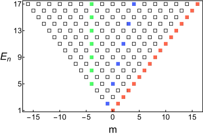
Figure 1: Energies (4) corresponding to normal modes (6) labeled by quantum numbers $n$ and $m$. A few possible restrictions to smaller sets of modes, addressed within the resonant approximation in section III, are highlighted by colors. The rightmost highlighted diagonal line is the lowest Landau-level truncation which was used in Ref. [30, 31]. The vertical highlighted line represents the fixed-angular-momentum truncations employed in Ref. [32]. The remaining highlighted line represents a generic restriction to a “one-dimensional” subset of modes that play a central role here, in sections IV and V.

One could try to perturbatively improve, as a power series in $g$, the linearized solutions of Eq. (2),

$$\Psi_{\mbox{\tiny linear}}(t,r,\phi)=\sum_{n,m}A_{nm}e^{-iE_{n}t}\Psi_{nm}(r,\phi),$$ (7)

where $\Psi_{nm}$ are the normal modes given by Eq. (6) and $A_{nm}$ are constant complex amplitudes. This approach is known to fail, however, due to the apprearance of secular terms that grow in time and lead to breakdown of the perturbative expansion on time scales $t\sim 1/|g|$. An appropriate alternative that correctly captures the dynamics on the relevant time scales is provided by the resonant approximation. To develop it, we start by decomposing exact solutions to Eq. (2) in terms of the linearized modes,

$$\Psi(t,r,\phi)=\sum_{n,m}\alpha_{nm}(t)\,e^{-iE_{n}t}\Psi_{nm}(r,\phi),$$ (8)

where $\alpha_{nm}$ are complex-valued functions of time. Plugging this decomposition in Eq. (2) and projecting onto $\Psi_{nm}$, one obtains an infinite system of ordinary differential equations,

$$i\frac{d\alpha_{nm}}{dt}=g\sum_{n_{i}m_{i}}C_{nn_{1}n_{2}n_{3}}^{mm_{1}m_{2}m_{3}}\bar{\alpha}_{n_{1}m_{1}}\alpha_{n_{2}m_{2}}\alpha_{n_{3}m_{3}}e^{-iEt},$$ (9)

where the bar stands for complex conjugation,

$$E\equiv E_{n}+E_{n_{1}}-E_{n_{2}}-E_{n_{3}},$$ (10)

and the interaction coefficients, or resonant mode couplings, are defined by

$$C_{nn_{1}n_{2}n_{3}}^{mm_{1}m_{2}m_{3}}\equiv\int_{0}^{\infty}rdr\int_{0}^{2\pi}d\phi~{}\bar{\Psi}_{nm}\bar{\Psi}_{n_{1}m_{1}}\Psi_{n_{2}m_{2}}\Psi_{n_{3}m_{3}}.$$ (11)

As the $\phi$-dependence of $\Psi_{nm}$ is given by $e^{im\phi}$, the $\phi$ integration nullifies $C$, unless

$$m+m_{1}=m_{2}+m_{3},$$ (12)

which represents the angular momentum conservation.

Note that we did not make use of the weakly nonlinear limit yet, and the expressions up to this point are correct for finite values of $g$. On the other hand, when $g$ is small the dynamics described by Eq. (9) acquires a conspicuous two-scale structure. Namely, most terms on the right-hand side come with oscillatory factors $e^{-iEt}$ that vary on time scales $t\sim 1$, while $\alpha_{nm}$ have time derivatives $\sim g$, thus varying slowly, on scales $t\sim 1/g$. It is natural to expect that the effect of the oscillatory terms averages out and may be neglected (a more precise statement is given below), while significant contributions to the evolution of $\alpha_{nm}$ are produced only by those terms on the right-hand side of Eq. (9) that do not oscillate on time scales $\sim 1$, which is precisely the terms with $E=0$, or

$$n+n_{1}=n_{2}+n_{3}.$$ (13)

The resonant approximation, so named after resonance condition (13), is defined by keeping only such non-oscillatory terms. Under this approximation, which is the main focus of our study, and introducing the slow time $\tau=gt$ (with overdots denoting $\tau$-derivatives from now on), one obtains the following resonant system of the 2D NLS/GP equation with the HO potential:

$$i\dot{\alpha}_{nm}=\underset{m+m_{1}=m_{2}+m_{2}}{\sum_{n+n_{1}=n_{2}+n_{3}}}C_{nn_{1}n_{2}n_{3}}^{mm_{1}m_{2}m_{3}}\bar{\alpha}_{n_{1}m_{1}}\alpha_{n_{2}m_{2}}\alpha_{n_{3}m_{3}}.$$ (14)

The general expectation is that Eq. (14) provides an accurate approximation to the exact evolution equations (9), which are tantamount to Eq. (2), over times $t\sim 1/g$. Such statements for systems of evolution equations with a finite number of degrees of freedom can be rigorously proved by elementary methods [25]. At the same time, a mathematically rigorous treatment of approximating the specific equation (2) by Eq. (14) is given in Ref. [27]. Resonant equations of this type have also been recently employed to study two-component BECs [57], as well as the scattering dynamics governed by NLS equations when the HO trapping only acts in a single spatial direction [58].

As mentioned above, 2D equation (2) has a specific symmetry structure, which becomes even more manifest in the resonant approximation. Thus, the evolution defined by Eq. (14) conserves the following six quantities [27]:

$${N} =\sum_{nm}\,|{\alpha}_{nm}|^{2},$$ (15)

$${M} =\sum_{nm}m\,|{\alpha}_{nm}|^{2},$$ (16)

$${E} =\sum_{nm}n\,|{\alpha}_{nm}|^{2},$$ (17)

$${Z}_{+} =\sum_{nm}\sqrt{\frac{n+m+2}{2}}\,{\bar{\alpha}}_{n+1,m+1}{\alpha}_{nm},$$ (18)

$${Z}_{-} =\sum_{nm}\sqrt{\frac{n-m+2}{2}}\,{\bar{\alpha}}_{n+1,m-1}{\alpha}_{nm},$$ (19)

$${W} =\sum_{nm}\frac{\sqrt{n^{2}-m^{2}}}{2}\,{\bar{\alpha}}_{nm}{\alpha}_{n-2,m}.$$ (20)

The first two of them are directly inherited from the conservation laws of Eq. (2) and correspond to the conservation of the wavefunction norm (number of particles) and angular momentum. The third one is related to the energy of the linearized version of Eq. (2), which is conserved by the resonant interactions retained in Eq. (14). Finally, the origin of the three remaining conserved quantities can be traced back [35] to the “breathing modes” of Eq. (2) — namely those quantities that evolve periodically for all solutions of the equations of motion. Thus, $Z_{+}$ and $Z_{-}$ correspond to the two spatial coordinates of the center-of-mass of the field configuration described by $\Psi(x,t)$, which always performs a simple harmonic oscillatory motion [59], while $W$ corresponds to the Pitaevskii-Rosch breathing mode [51, 52].

We finally quote an explicit expression for the interaction coefficients (11) through the Laguerre polynomials:

$$C_{n_{1}n_{2}n_{3}n_{4}}^{m_{1}m_{2}m_{3}m_{4}}=\frac{1}{\pi}\left(\prod_{i=1}^{4}\sqrt{\frac{(\frac{1}{2}(n_{i}-m_{i}))!}{(\frac{1}{2}(n_{i}+m_{i}))!}}\right)$$ (21)

$$\times\int_{0}^{\infty}d\rho\,e^{-2\rho}\rho^{(m_{1}+m_{2}+m_{3}+m_{4})/2}\left(\prod_{i=1}^{4}L_{\frac{n_{i}-m_{i}}{2}}^{m_{i}}(\rho)\right).$$

As the Laguerre polynomials are generated by a simple iterative procedure that raises their degree (related to the raising operators for the HO), these interaction coefficients inherit a peculiar discrete structure from the underlying set of eigenmodes. In particular, they satisfy a set of simple finite-difference equations [33, 36] linked to the conservation laws (18-20). Integrals in Eq. (21) are known as Krein functionals in mathematical literature [60], some of them featuring prominently in combinatorics [61, 62]. The discrete nature of the integrals of products of Laguerre polynomials spawns a profusion of identities for the interaction coefficients that, in turn, translate into peculiar dynamical patterns in the resonant evolution described by Eq. (14), some of which are considered below.

III Restriction of the resonant evolution to subsets of modes

The resonant evolution governed by Eq. (14) can be consistently restricted to various subsets of modes in the sense that, if the initial data excite only modes in a particular subset of this sort, no modes outside the subset will be excited at later times if the system evolves according to Eq. (14). Since the novel dynamical phenomena that we report in this article unfold within such restrictions, it is relevant to review this aspect of the model first.

The key aspect of Eq. (14) that supplies a large variety of consistent dynamical restrictions is the presence of both the resonance condition $n+n_{1}=n_{2}+n_{3}$ and the conservation condition for the angular momentum, $m+m_{1}=m_{2}+m_{3}$ in the summation on the right-hand side. As a result, if $(n_{1},m_{1})$, $(n_{2},m_{2})$ and $(n_{3},m_{3})$ satisfy $an_{j}+bm_{j}=c$, for $j=1,2,3$, with arbitrary $a$, $b$, $c$, then $(n,m)$ satisfies the same equation. Thus, if the initial state excites exclusively modes $\alpha_{nm}$ with $an+bm=c$, the time derivatives of $\alpha_{nm}$ in Eq. (14) vanish for all modes $\alpha_{nm}$ with $an+bm\neq c$, hence those modes will permanently keep zero values. One can thus consistently restrict the resonant evolution to any straight line traversing the mode tower in Fig. 1, a few such restrictions having been highlighted in that figure.

The restrictions reduce the number of indices of modes $\alpha_{nm}$ from two to one, as $n=n(l)$ and $m=m(l)$ are now linear functions of the new mode index $l$, hence one can introduce $\alpha_{l}\equiv\alpha_{n(l)m(l)}$. The two conditions $n+n_{1}=n_{2}+n_{3}$ and $m+m_{1}=m_{2}+m_{3}$ in Eq. (14) now coalesce into a single resonance condition, $l+l_{1}=l_{2}+l_{3}$, and, under the adopted mode restriction, one can rewrite Eq. (14) as

$$i\dot{\alpha}_{l}=\sum_{l+k=i+j}C_{lkij}\bar{\alpha}_{k}\alpha_{i}\alpha_{j}.$$ (22)

There is a further dynamical restriction that one can impose, namely, if the initial state only excites $\alpha_{l}$ with $l=p\mod q$, then no $\alpha_{l}$ with $l\neq p\mod q$ will get excited. Thus, not only can one restrict to straight lines within the mode tower, as in Fig. 1, but it is also possible to further restrict the evolution to any regular 1D lattice of modes positioned along any given straight line.

The full variety of such restrictions is conveniently characterized by the two lowest modes $(n_{0},m_{0})$ and $(n_{1},m_{1})$. Once these modes have been selected, the full set of modes $\alpha_{l}\equiv\alpha_{n(l)m(l)}$ that participate in the evolution is defined by $n(l)=n_{0}+(n_{1}-n_{0})l$ and $m(l)=m_{0}+(m_{1}-m_{0})l$, and the evolution equation can be written as

$$i\dot{\alpha}_{l}=\sum_{k=0}^{\infty}\sum_{i=0}^{l+k}C_{lki,l+k-i}\bar{\alpha}_{k}\alpha_{i}\alpha_{l+k-i},$$ (23)

where we have converted the resonance condition $l+k=i+j$ into an explicit specification of the summation ranges. The interaction coefficients in this restricted resonant system are inherited from Eq. (21) as $C_{lkij}\equiv C_{n(l)n(k)n(i)n(j)}^{m(l)m(k)m(i)m(j)}$. Note that the interaction coefficients satisfy $C_{lkij}=C_{lkji}=\bar{C}_{ijlk}$.

Within the restriction given by Eq. (23), the conserved quantities (15-20) reduce to a smaller set. The first quantity is directly carried over to Eq. (23), while the second and third ones merge into a single conserved quantity, due to the linear relation between $n$ and $m$ imposed by the mode restriction. As a result, one is left with two quantities conserved by Eq. (23):

$$N=\sum_{l=0}^{\infty}|\alpha_{l}|^{2},\qquad E=\sum_{l=1}^{\infty}l\,|\alpha_{l}|^{2}.$$ (24)

The symmetry transformations corresponding to these conservation laws are

$$\alpha_{l}\rightarrow e^{i\eta}\alpha_{l}\quad\mbox{and}\quad\alpha_{l}\rightarrow e^{i\theta l}\alpha_{l},$$ (25)

where $\eta$ and $\theta$ are $l$-independent parameters. As to the remaining three conservation laws (18-20), they degenerate to identical zeros for generic straight-line restrictions in Fig. 1. Exceptions to this rule are given by restrictions along diagonal lines directed at $45^{\circ}$ in Fig. 1 (the Landau levels), that retain either $Z_{+}$ or $Z_{-}$ [30, 32], or vertical lines (angular momentum levels) that retain nonzero $W$ [32]. The surviving conservation laws have strong consequences for these specific restrictions [30, 32], but they are not present in the case of generic restrictions that will be our focus below.

In our treatment, we are mainly concerned with restrictions corresponding to straight lines in Fig. 1 forming angles $>45^{\circ}$ with the horizontal axis. Restrictions to straight lines at angles $<45^{\circ}$ are certainly possible, but they are less relevant in relation to topics of energy transfer, since these restrictions necessarily involve only a finite set of modes.

Under each specific mode restriction described by Eq. (23), we will mostly work with the two-mode initial data,

$$|\alpha_{0}(0)|\neq 0,\quad|\alpha_{1}(0)|\neq 0,\quad|\alpha_{l\geq 2}(0)|=0.$$ (26)

In terms of the original mode tower of Fig. 1, this corresponds to exciting two modes $(n_{0},m_{0})$ and $(n_{1},m_{1})$ and tracking the subsequent evolution. Such two-mode initial data are the simplest setup leading to nontrivial evolution, as single-mode initial data never induce any energy exchange between the modes in the course of the resonant evolution defined by Eq. (14). The dynamical trajectories starting with two-mode initial data can, on the other hand, display very elaborate behaviors. They have been often studied in the context of resonant systems of the type of Eq. (23), not necessarily related to the present setup, and have been seen to result, in different situations, in perfectly periodic evolution of the mode amplitude spectrum [30, 32, 33, 49, 44, 63, 43], turbulent phenomena [63, 64, 48] and FPU-like approximate energy returns [41, 42]. Our purpose in the following two sections is to examine the energy transfer patterns resulting from two-mode initial data specifically in the context of the resonant system (14), derived from the NLS/GP equation with the isotropic HO potential (2), and identify FPU-like recurrencies in this setting, as well as special two-mode initial data for which the energy transfer is completely blocked by the structure of the interaction coefficients (21).

IV Dynamical revivals

To put things in perspective, we pause for a moment and discuss what kind of behavior one may expect from systems of the form of Eq. (23), starting with the two-mode initial conditions (26), before specializing to the actual values of the interaction coefficients $C$ arising from the NLS equation (2). Initially, the energy leaves the two lowest modes and spreads to the higher ones, which is often described as a “turbulent cascade”, as the energy flows towards shorter wavelengths. The strength of the turbulent cascade varies widely depending on the precise set of interaction coefficients $C$ [65]. In extreme cases, the cascade leads to formation of a power-law spectrum in a finite time, known as the “finite-time turbulent blowup” [48, 64]. More conventionally, as is the case for the low-dimensional NLS equations that we address here, the direct cascade only lasts over a finite time period, whereupon it halts and turns into a reverse cascade driving the energy back to the low-lying modes. Note that, due to the presence of the doublet of conservation laws (24), the direct cascade is itself of a dual nature [66], meaning that there is a simultaneous flow of energy both to higher and lower modes, since it is the only way to ensure that both quantities (24) are conserved.

The efficiency of the reverse cascade also varies from one system to another and among different initial conditions. For some specific mode restrictions given by Eq. (14), such as the Landau-level [30, 32] and fixed-angular-momentum [32] restrictions highlighted in Fig. 1, if the evolution starts with the two-mode initial data (26), the direct cascade is followed by a reverse one that brings the mode energies back exactly to the initial configuration. The process then simply repeats itself periodically. Such perfect dynamical recurrencies are of course highly non-generic, and they are mandated by the enhanced symmetry structures [33, 35, 37] that operate within these specific mode restrictions.

For more generic mode restrictions in Fig. 1, which do not go vertically or diagonally at $45^{\circ}$, there are no reasons to expect that the reverse cascade will perfectly restore the initial mode energy distribution, and, indeed, numerical simulations of Eq. (23) show that such perfect restoration does not occur. At the same time, one observes that, for many specific restrictions, the mode energy distribution at the bottom of the reverse cascade comes very close to the initial configuration (26), very much in the spirit of the FPU phenomena [39, 40] in nonlinear oscillator chains. Reporting such dynamical behaviors is one of the main strands of our presentation. Below we give a heuristic argument to explain why such FPU-like behaviors may be generically expected in systems of the form of Eqs. (23), although the actual precision of the revival by the reverse cascade of the original amplitude spectrum cannot be accurately determined from such arguments, requiring case-by-case numerical simulations. Note that the direct-reverse cascade sequences continue past the first turbulent oscillation that we have outlined above, and later reverse cascades may restore the initial amplitude spectrum with an even better precision than the first one, which is also what had happens in the original FPU setup.

In what follows, we choose two modes $(n_{0},m_{0})$ and $(n_{1},m_{1})$, as in the previous section, and launch simulations of Eq. (14) with only these two modes excited in the initial state. As per discussion in the previous section, the subsequent evolution excites only modes positioned along the straight line passing through the points $(n_{0},m_{0})$ and $(n_{1},m_{1})$ in Fig. 1, for which the restricted resonant equation (23) may be applied, where the two initially excited modes are simply relabelled as mode 0 and mode 1. To quantify the FPU-like phenomena, we measure the contribution to the “particle number” $N$ in Eq. (24) from modes higher than those corresponding to $l=1$:

$$\Delta(\tau)\equiv\sum_{l=2}^{\infty}|\alpha_{l}(\tau)|^{2}.$$ (27)

Initially, this is zero by construction, then it starts growing in the course of the first direct cascade, and we subsequently track the minima of this function at later times, brought about by the reverse cascades. The ratio $\Delta_{\min}/\Delta_{\max}$ of the minimum and maximum of $\Delta$ provides a characterization of the prominence of the FPU phenomena.

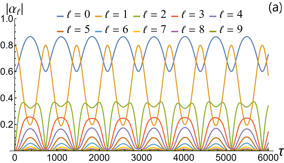
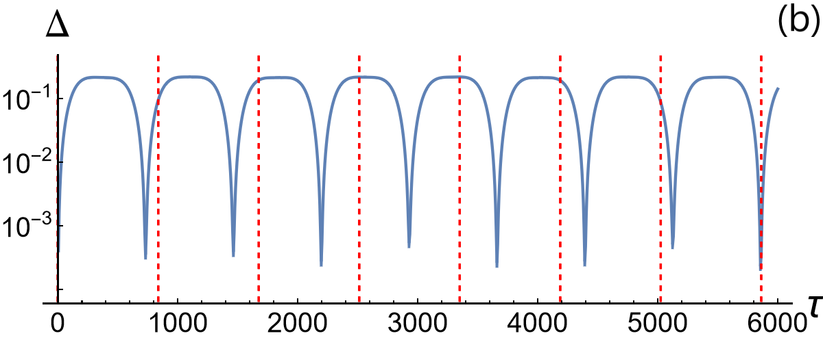
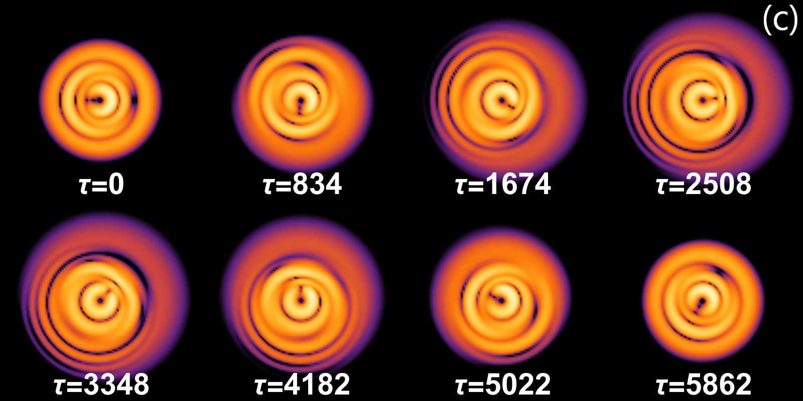
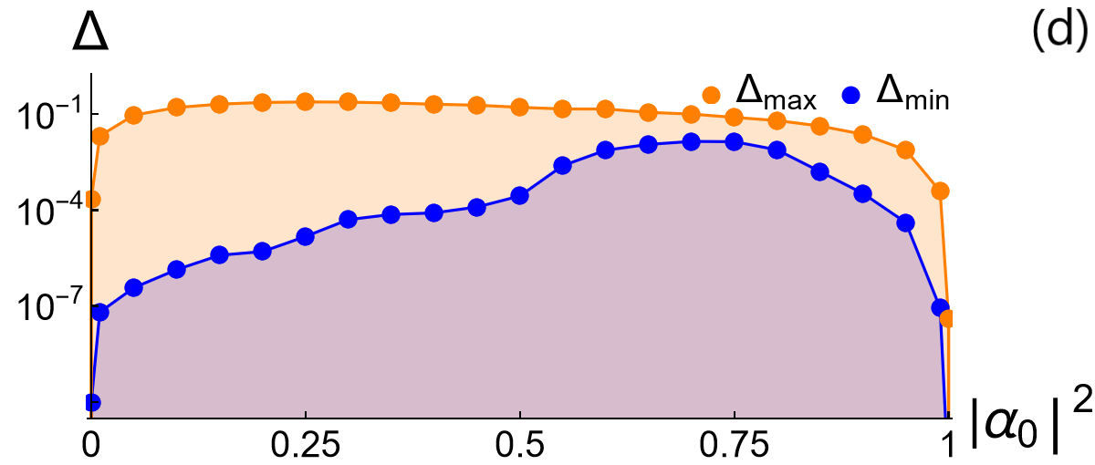
Figure 2: The upper plot: the evolution of $|\alpha_{l}|$. The second plot: the contribution to $N$ from modes with ${\small l>1}$, defined as per Eq. (27). The third plot: the position-space representation of $|\psi|^{2}$ at times highlighted by red dashed lines in the middle plot. The initial configuration consists of the two-mode initial data (26). The two modes in the initial state in these plots are chosen as $(n_{0},m_{0})=(4,-2)$ and $(n_{1},m_{1})=(9,-3)$ with initial values $\alpha_{0}=0.6$ and $\alpha_{1}=0.8$, such that Eq. (24) gives $N=1$. The lower plot: the maximum and minimum values of $\Delta(\tau)$ over a succession of $50$ direct-reverse cascades (with the first direct cascade excluded) for the restriction given in the upper plots but different distributions of the initial energy between modes 0 and 1 (with $N=1$).

We note that the dynamics of two-mode initial data (26) is determined by the initial amplitudes $|\alpha_{0}|$ and $|\alpha_{1}|$, as the phases of these two modes can be rotated arbitrarily by the symmetry transformations (25). In the position space picture, such phase changes are seen as a rotation of the wavefunction density around the origin. Thus, if a perfect return to the initial configuration of $|\alpha_{0}|$ and $|\alpha_{1}|$ occurs, one sees a rotated version of the initial configuration. The subsequent evolution will, of course, repeat the first-pass revival as transformations (25) are symmetries of the resonant evolution (23), while the spatial rotations are a symmetry of the original PDE (2). If approximate (rather than perfect) revivals of the initial two-mode configuration occur, this scenario will still be in operation, up to small distortions.

Figure 2 shows a representative example produced by the simulations, while a few extra plots are given in Appendix A. We observe that the evolution of $|\alpha_{l}(\tau)|$ displays oscillations in the form of direct-reverse cascade sequences, and the energy, initially located in modes $0$ and $1$, is transferred to higher modes, followed by accurate returns. In the case shown in Fig. 2 this process is so accurate that it is difficult to distinguish it from exact periodicity in a straightforward graphic presentation. The initial direct cascade spreads the energy appreciably, so that one gets $\Delta>0.1$, but at later times the initial configuration is re-assembled with precision as good as $\Delta\sim 10^{-4}$. In the corresponding picture of the wavefunction density distribution in the position-space representation, defined in terms of

$$\psi(\tau,r,\phi)\equiv\sum_{n,m}\alpha_{nm}(\tau)\,\Psi_{nm}(r,\phi),$$ (28)

one sees that the initial distribution is appreciably deformed and then recovered with a nearly-perfect precision (the picture gets rotated after this recovery since, while the amplitudes $|\alpha_{nm}|$ return almost exactly to their initial values, the phases $\arg(\alpha_{nm})$ undergo a drift). Note that (28) is defined in terms of the slow-time evolution on time scales $t\sim 1/g$. To convert it to the wavefunction (8) of the original equation (2), one must apply the evolution operator of the linear quantum HO to $\psi(\tau=gt)$.

It is possible to gain further insight into the FPU phenomena in resonant system (23) by considering initial conditions where one of the two modes in the initial state (26) dominates. This analysis is similar to that developed in Ref. [42] for related relativistic systems, where more detailed and in-depth considerations were reported. We choose for the presentation here the simpler case when the dominant mode is the one labeled as mode $0$. The direct cascade is expected to be weak in this case, as follows a posteriori from the consistency of our analysis presented below, and is easy to verify numerically. In this situation, it is natural to assume a strong exponential suppression of the spectrum in the form of

$$\alpha_{n}=\delta^{n}\,q_{n}(\tau),$$ (29)

with a small free parameter $\delta$. One can then treat the evolution of this form at leading order in $\delta$, which results in a simplified system,

$$i\dot{q}_{n}=\bar{q}_{0}(t)\sum_{k=0}^{n}C_{n0k,n-k}q_{k}q_{n-k}.$$ (30)

Unlike the original resonant system (23), equations with lower $n$ now decouple from the higher ones, and Eq. (30) can be solved recursively mode-by-mode. We can set $q_{0}(0)=1$, using the scaling symmetry of Eq. (23) of the form $\alpha(\tau)\rightarrow\lambda\alpha(\lambda^{2}\tau)$, and $q_{1}(0)=1$, adjusting the definition of $\delta$. Then, in the framework of Eq. (30), the first two modes simply oscillate as

$$q_{0}(t)=e^{-iC_{0000}\tau},\qquad q_{1}(t)=e^{-iC_{0101}\tau},$$ (31)

while higher $q_{n}$ satisfy

$$i\dot{q}_{n}-2C_{0n0n}q_{n}=\bar{q}_{0}\sum_{k=1}^{n-1}C_{n0k,n-k}q_{k}q_{n-k},$$ (32)

where the right-hand side only depends on $q_{k}$ with ${k<n}$, which have already been evaluated at the previous iterative steps, hence they simply provide a source term for the oscillations of $q_{n}$. As a result, each $q_{n}$ is a sum of oscillatory terms proportional to $e^{i\Omega\tau}$, where, for every such term, $\Omega$ is a linear combination of $C_{0k0k}$ with integer coefficients, and only for $k\leq n$. For completeness, we mention that it is in principle possible for $q_{n}$ to contain secular terms growing like $\tau e^{i\Omega\tau}$ when the right-hand side of (32) happens to contain a term that oscillates with frequency $2C_{0n0n}$. Such behavior occurs in specific situations where instabilities are present, and has no bearing on the bulk of our considerations.

From the perspective of Eq. (32), FPU phenomena enter the stage naturally in the following manner. Solving Eq. (32) for $q_{2}$, with initial condition $q_{2}(0)=0$, yields

$$|q_{2}|\sim\sin\left(\frac{1}{2}(C_{0000}-4C_{1010}+2C_{2020})\tau\right),$$ (33)

which shows that $q_{2}$ periodically vanishes. When this happens, the energy is entirely concentrated in modes $0$ and $1$, except for the contributions in modes $3$ and higher, suppressed by $\delta^{6}$. This is simply a reflection of a single direct-reverse cascade return in the limit of small $\delta$. More accurate returns may occur at later times. The point is that, due to the special nature of the interaction coefficients (21) expressed through a highly structured family of orthogonal polynomials, many of these coefficients are rational numbers. We exhibit below specific mode restrictions leading from Eq. (14) to Eq. (23) such that all coefficients $C_{0n0n}$ are rational numbers in units of $C_{0000}$. If all $C_{0n0n}$ are rational in units of $C_{0000}$, then the solutions for all $q_{n}$ are superpositions of oscillations with rational frequencies, which means that any finite subset of $q_{n}$ has a common period. For example, it is guaranteed that a moment of time exists when $q_{2}$ and $q_{3}$ will return to the initial configuration, where they both vanish. At that moment, the energy returns to modes $0$ and $1$ with precision $\delta^{8}$. Even more broadly, for those mode restrictions where $C_{0n0n}$ are not all rational, approximate common periods may exist, securing dynamical returns with enhanced precision, as discussed in Ref. [42].

We now present a specific simple family of mode restrictions where the picture outlined above plays a role. In this family, mode $0$ is chosen to be $(n_{0},m_{0})=(0,0)$ and mode $1$ is any other mode $(n,m)$. Then, mode number $l$ is $(nl,ml)$. We claim that, under this restriction, the following relation holds:

$$\frac{C_{0l0l}}{C_{0000}}=\frac{(nl)!}{2^{nl}\left(\frac{1}{2}(n+m)l\right)!\left(\frac{1}{2}(n-m)l\right)!},$$ (34)

hence all $C_{0l0l}$ have rational values in units of $C_{0000}$. Thus, synchronization takes place between periods of different modes in Eq. (32), providing for returns with improved precision. A derivation of Eq. (34) is given in appendix B.

Of course, our analysis of the dynamics close to mode $0$ is only valid at its face value when mode $1$ is strongly suppressed in the initial configuration. However, it does provide correct intuition in relation to the direct-reverse cascade sequences produced by Eq. (23), and allows one to predict which numbers of direct-reverse cascades result in particularly accurate returns. These predictions, furthermore, continue to hold even for initial conditions where modes $0$ and $1$ carry comparable energies, as has been demonstrated by detailed analysis of a related resonant system in [42].

Similar considerations are possible for dynamical trajectories dominated by mode $1$ [42]. In that case, instead of relation (29), one assumes a $\delta$-dependence in the form of $\alpha_{0}=\delta q_{0}$, $\alpha_{l\geq 1}=\delta^{l-1}q_{l}$. This specification of $\delta$-dependencies is consistent in the sense that, upon the substitution into resonant system (23) and taking the limit $\delta\rightarrow 0$, one obtains a simplified and yet nontrivial dynamical system for $q_{l}$, which can be analyzed by methods similar to the ones employed above for solutions dominated by mode $0$. This results in a picture of direct-reverse cascade sequences, as well as dynamical returns of enhanced precision. Further details can be recovered from Ref. [42].

The fact that the FPU behaviors (which can be naturally explained in a quantitative manner for initial conditions dominated by one of the two modes) persist for initial conditions with comparable mode energies remains an empirical observation. We have observed such returns for a number of choices of the initial configurations with comparable energies of the initially excited modes, as documented by Fig. 2 and further simulations presented in appendix A. It can be seen as a manifestation of the special character of the 2D NLS/GP equation (2) that the FPU behaviors, while being rather generic for initial data dominated by a single mode, extend, in the case of this equation, to a broader range of initial conditions. Pronounced FPU phenomena with $\Delta_{\min}/\Delta_{\max}\sim 10^{-4}$ have been observed in our simulations for initial data with the following pairs of modes $(n_{0},m_{0})$-$(n_{1},m_{1})$: (0,0)-(3,1); (0,0)-(4,2); (0,0)-(5,3); (1,-1)-(4,-2); (1,-1)-(4,2); (1,-1)-(6,0); (2,0)-(6,0); (2,0)-(5,1); (2,-2)-(5,-1); (2,-2)-(6,-4); (4,-2)-(9,-3); (4,-2)-(7,-1). These observations suggest that dynamical recurrencies are not uncommon in the evolution governed by Eq. (14).

V Two-mode persistent breathers

In our searches for FPU behaviors within various mode restrictions imposed on Eq. (14), we have discovered some initial conditions that lead to an even more dramatic failure of the energy redistribution among the normal modes. Rather than repeatedly returning to the vicinity of the original configuration, the energy for such initial conditions does not get transferred at all, at any time. We have already mentioned that this property holds in solutions of Eq. (14) for all single-mode initial conditions, but it does not generically hold for two-mode initial conditions. We have, however, discovered some special choices of two-mode initial conditions for which no energy transfer occurs in the course of the resonant evolution of Eq. (14).

The evolution with two-mode initial conditions always unfolds within one of the mode restrictions defined as per Eq. (23), namely, the restriction to the modes that fall onto the straight line passing through the two initially excited modes in Fig. 1. The energy transfer in (23) is blocked whenever the initial conditions are of the form (26) and the interaction coefficient $C_{2011}=0$. Indeed, for the initial conditions of this form, $\dot{\alpha}_{l}(0)$ with $l\geq 3$ are identically zero since each term on the right-hand side of (23) involves at least one of the initially vanishing modes $\alpha_{l}$ with $l\geq 2$. On the other hand,

$$i\dot{\alpha}_{2}(0)=C_{2011}\,\bar{\alpha}_{0}(0)\,\alpha_{1}^{2}(0).$$ (35)

Thus, the inception of energy transfer entirely hinges on $C_{2011}$. If this coefficient vanishes, then neither mode $2$ nor any higher ones get excited at the start of the evolution, hence they cannot be excited at any later stage either, with the evolution perpetually locked within the ansatz (26).

We have identified the following large family of two-mode initial data for which the corresponding coefficient $C_{2011}$ vanishes:

$$(n_{0},m_{0})=(2i+1,-(2j+1))\quad(n_{1},m_{1})=(2k,0)$$ (36)

with $j\leq i<k$ (to ensure that $(n_{0},m_{0})$ is indeed the lowest mode of the given restriction, one must supplement this condition with an extra requirement that $2(i-j)<k$). We provide a (relatively involved) proof for the vanishing of $C_{2011}$ corresponding to this family in appendix C. We have additionally observed the following more sparse families involving high-frequency modes that share the same property:

$$(n_{0},m_{0})=(2,0),\quad(n_{1},m_{1})=(k^{2},k)$$ (37)

and

$$(n_{0},m_{0})=(k^{2}-k,-k^{2}+k+2),\quad(n_{1},m_{1})=(k^{2},k)$$ (38)

with $k=2,3,4,...$. Evidently, the sign of the angular momentum can be flipped in all of these families due to the reflection symmetry.

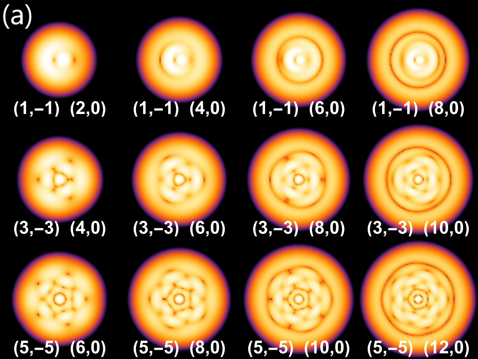
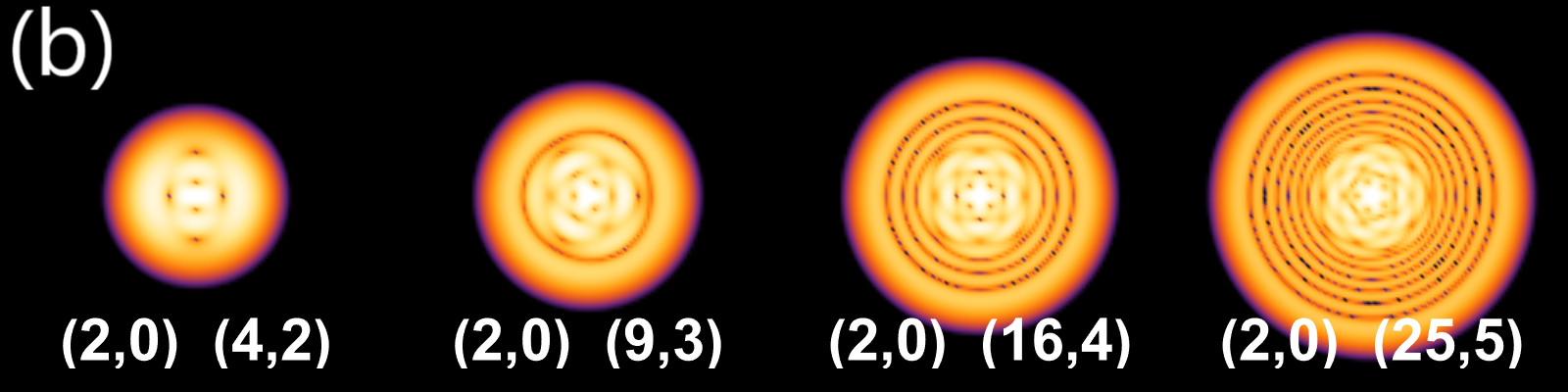
Figure 3: The spatial configuration of $|\psi|^{2}$ in the stationary solutions given by Eqs. (36) (rows from 1 to 3, (a)) and (37) (the lower row, (b)). Each plot specifies two excited modes $(n_{0},m_{0})$ and $(n_{1},m_{1})$, as indicated by white numbers.

A collection of position space distributions of the wavefunction density obtained from Eq. (28) for these two-mode configurations is plotted in Fig. 3. Note that the complex amplitudes of the two modes activated in the initial state may be prescribed arbitrarily for each specification of the integer parameters that define the above two-mode families. While within the resonant approximation (14) these configurations are exactly stationary in the sense that $|\alpha_{n_{0}m_{0}}|^{2}$ and $|\alpha_{n_{1}m_{1}}|^{2}$ are frozen in time, while all other modes remain zero, the corresponding initial data in the original PDE (2) will lead to some evolution, but only in an extremely slow form at small $g$. On time scales $t\gg 1/g$, the resonant approximation ceases to be accurate and solutions of (2) may drift away from these predictions. Yet on time scales $t\sim 1/g$, the initial data in the form of Eq. (36-37) continue tracking the linearized evolution very closely, forming a long-lived breather-like stationary pattern. This behavior is strongly non-generic for weakly nonlinear NLS/GP equations (2) with abundant normal-mode resonances.

To put our finding of two-mode stationary solutions in perspective, we further remark that resonant systems of the form (23) generically possess stationary solutions without energy transfer. These solutions have spectra given by $\alpha_{n}=e^{i(\omega+n\lambda)\tau}A_{n}$, where $A_{n}$ are $\tau$-independent and depend on $C_{nmkl}$ (upon substituting this ansatz into (23), all the $\tau$-dependent factors drop out, leaving a system of algebraic equations for $\omega$, $\lambda$ and $A_{n}$.) Such solutions, however, generically have infinitely many modes turned on, with a very specific arrangement of amplitudes and phases, and would be difficult to recreate. The two-mode stationary solutions we report here are, by contrast, specific to the model we consider, and their existence relies on the vanishing of particular four-mode couplings, which is a special feature of the NLS/GP equation (2).

VI Conclusion

We have considered the long-term weakly nonlinear evolution of the 2D NLS/GP equation with the isotropic HO (harmonic oscillator) potential. The analysis has revealed an array of FPU phenomena and stationary configurations in this regime. Our findings further highlight the special nature of the low-dimensional NLS/GP equations with the HO potentials, which previously exhibited other unusual dynamical behaviors [12, 7, 13, 15, 16, 30, 32]. There are further physical connections between such behaviors and obstructions to ergodicity in low-dimensional many-boson systems in HO potentials [17, 18, 19], as all such phenomena originate from failures of effective redistribution of energy among the dynamical degrees of freedom.

It would be interesting to observe the dynamical patterns that we have displayed here in the evolution of trapped ultracold atomic gases, where HO potentials are routinely used, while the strength of the interactions can be adjusted by means of the Feshbach resonances. Detailed control over the preparation of the initial configurations remains a challenge, but it has been a focal point in recent research and substantial progress can be seen in experimental work [13].

In the context of nonlinear optics, both our 2D setup (corresponding to the transverse geometry of the waveguide) and the weakly nonlinear regime are very natural. In particular, considerations of the coexistence of a large number of transverse modes when nonlinearities are weak are highly relevant for the implementation of spatial-division-multiplexing schemes in optical data-transmission links [67]. HO potentials are less common in this setting, but they may be relevant too [22]. Note that the stationary solutions found in section V are distinguished by their quasi-linear evolution on long time scales, despite the fact that even weak nonlinearities could in principle generate large effects through the resonant interactions.

In a more speculative mode, one can try to employ the FPU phenomena in a sort of cryptographic scenario, with the communication line passing through an area where the transmission may be tapped. In this case, one could adjust the operation mode in such a way that the nonlinearities scramble the signal in the intermediate region (where the energy distribution of the initial signal is driven to the excited transverse modes by nonlinear interactions), and then the original transmission gets reconstructed by an FPU return at the read-out point. Even within our simple two-mode specification for the initial states used in section IV, the relative energy of the two modes can be used to transmit data, while the overall power of the signal can be used to ensure that the FPU recurrence takes place precisely at the specified read-out point.

Appendix A Additional numerical simulations

We complement the presentation in section IV with Fig. 4 containing a compilation of extra plots produced by our simulations. These plots contain a number of cases where the general scenario outlined in section IV is reproduced in detail, as well as some examples where the FPU returns are less pronounced. There is also a particular truncation where the single-mode solution supported by mode 1 is unstable, leading to a breakdown of the picture of strong exponential suppression in the spectra originating from initial data dominated by one mode. With all of these exceptions, FPU returns remain rather generic in the setup of this paper, and we have observed accurate returns in truncations defined by $(n_{0},m_{0})$-$(n_{1},m_{1})$: (0,0)-(3,1); (0,0)-(4,2); (0,0)-(5,3); (1,-1)-(4,-2); (1,-1)-(4,2); (1,-1)-(6,0); (2,0)-(6,0); (2,0)-(5,1); (2,-2)-(5,-1); (2,-2)-(6,-4); (4,-2)-(9,-3); (4,-2)-(7,-1), as already mentioned in the main text.

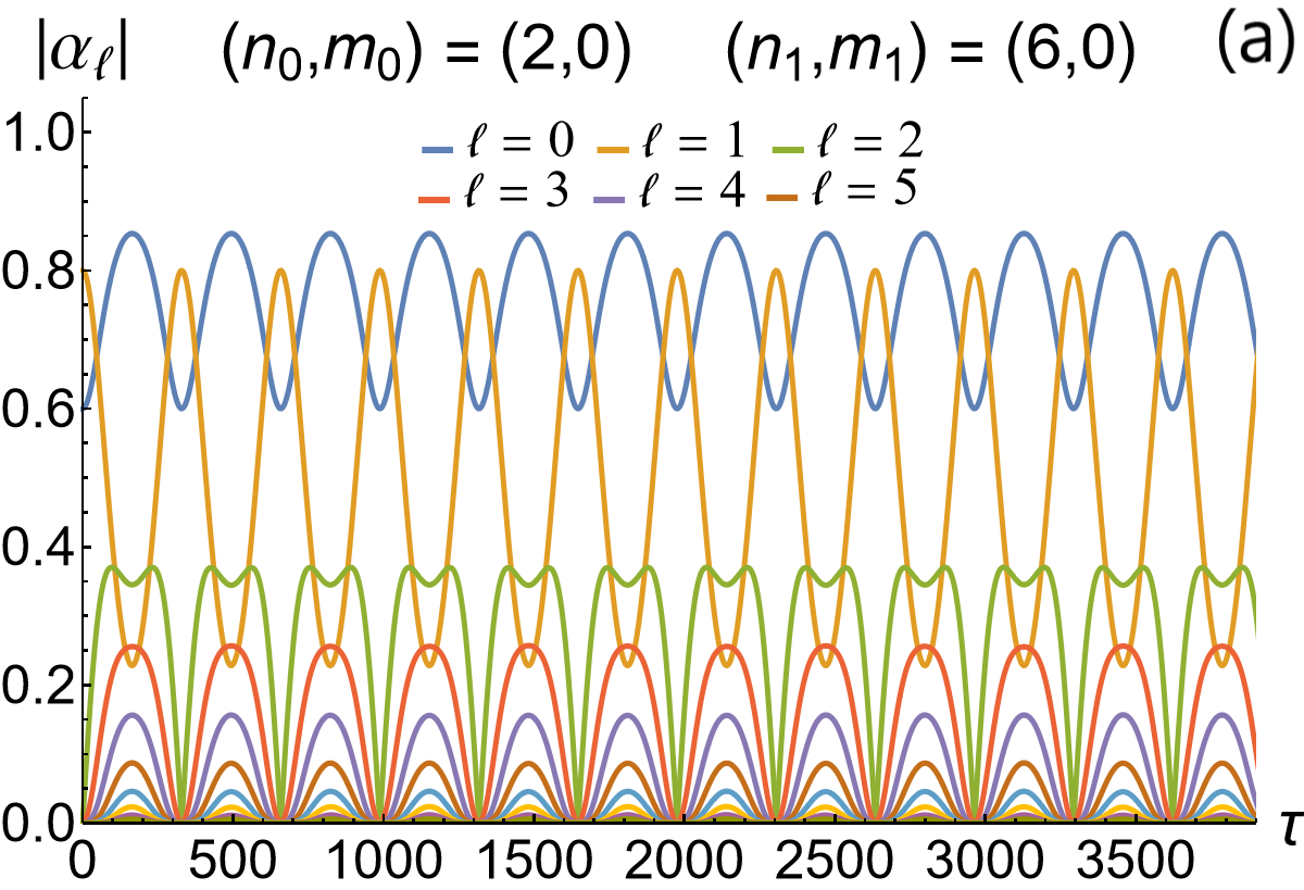
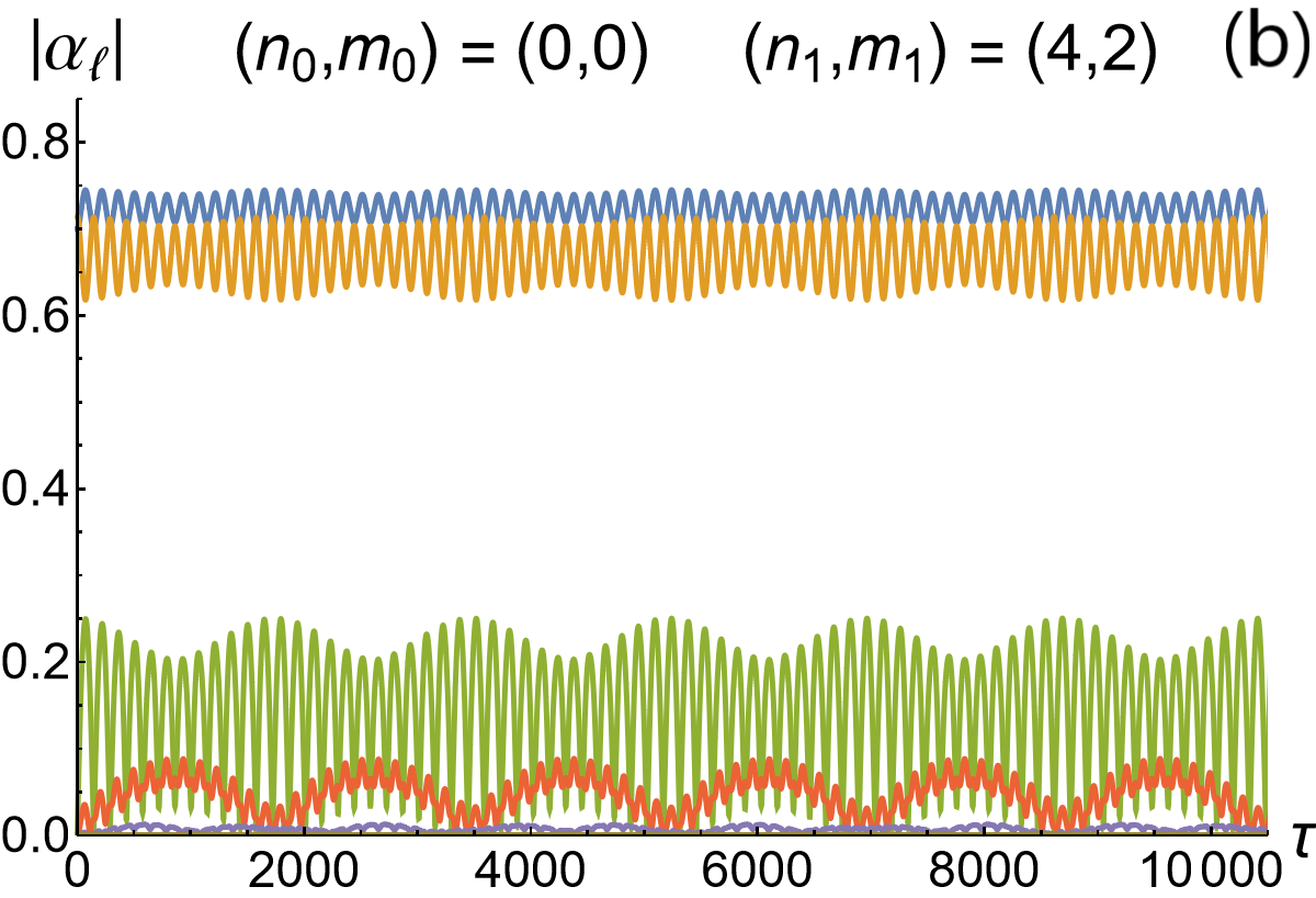
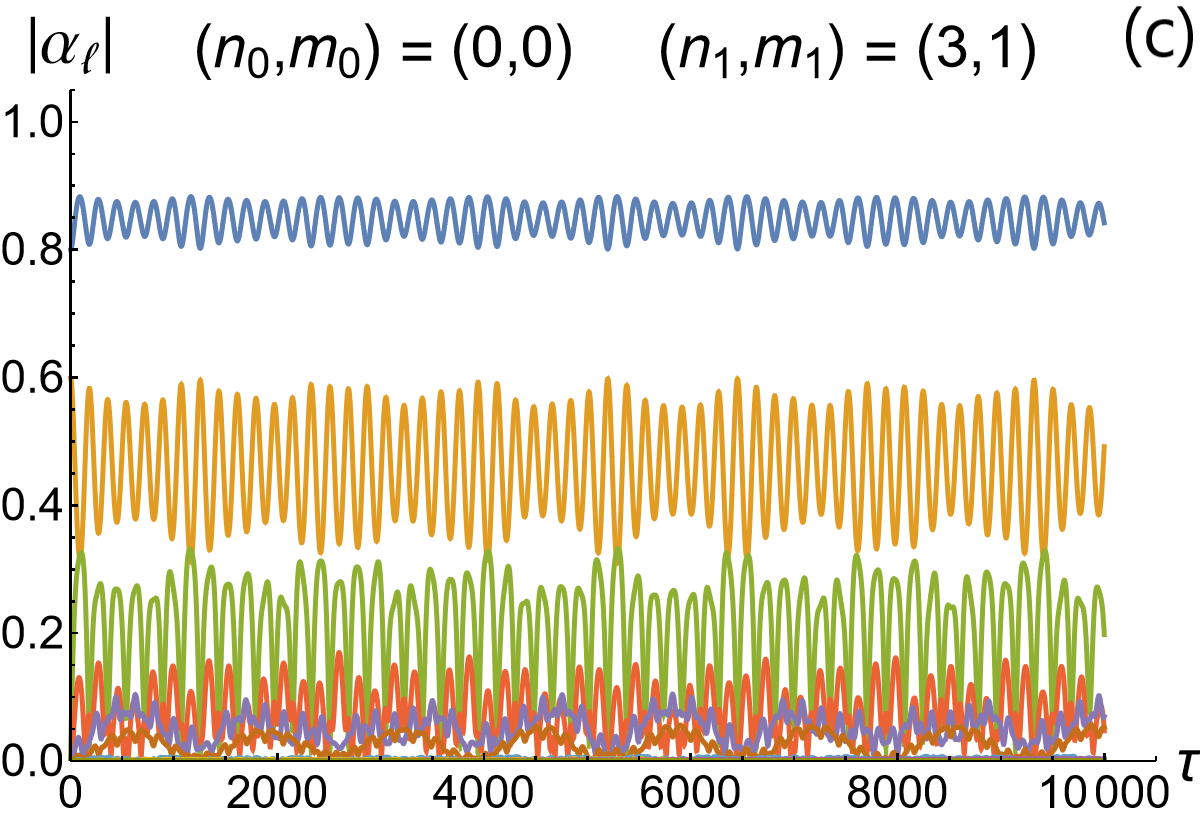
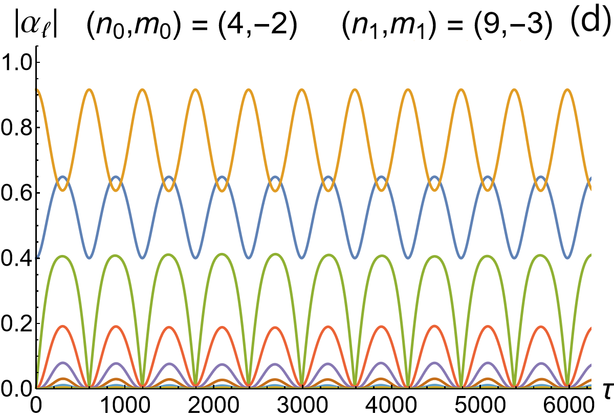
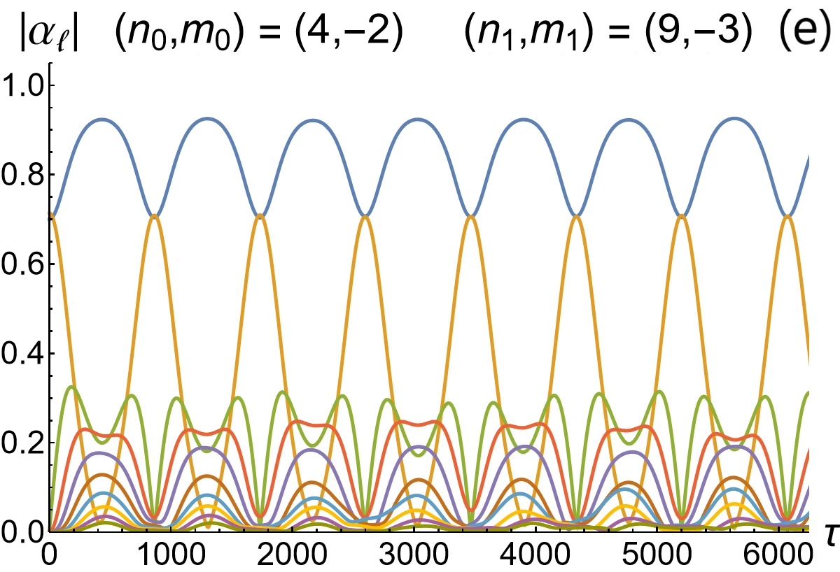
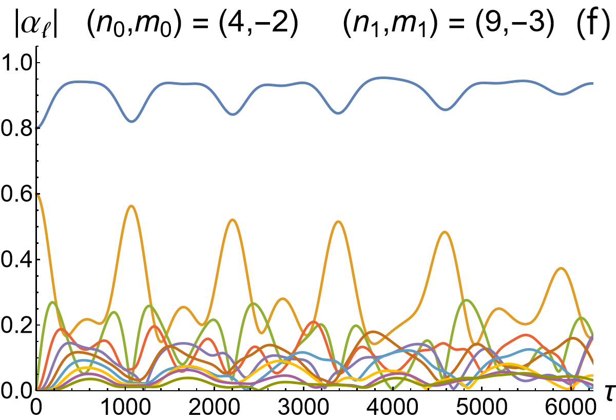
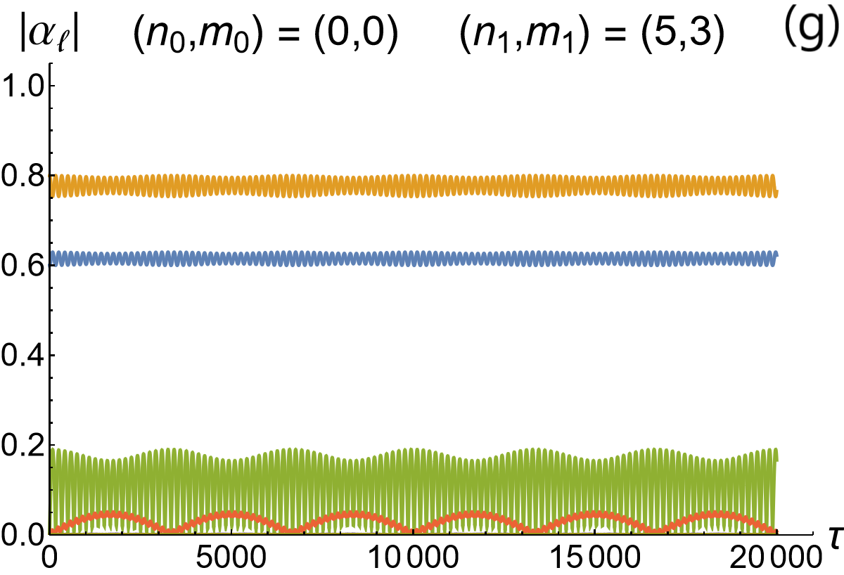
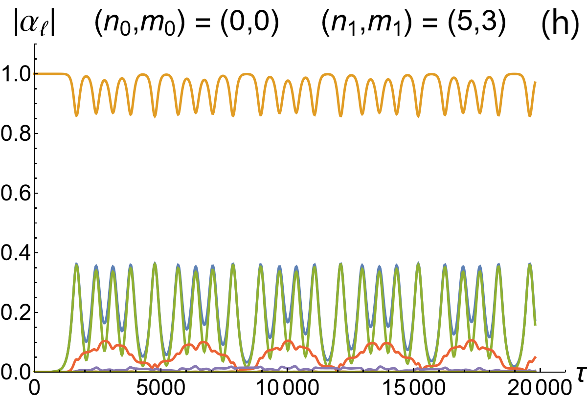
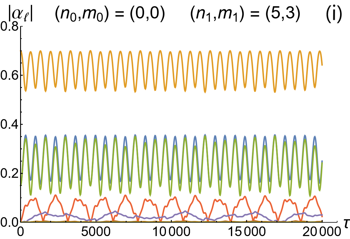
Figure 4: Upper row: The evolution within different mode restrictions (specified in each plot) that exhibit accurate energy returns for some two-mode initial data; from left to right $(\alpha_{0},\alpha_{1})=(0.6,0.8)$, $(\alpha_{0},\alpha_{1})=(0.7,0.7)$, and $(\alpha_{0},\alpha_{1})=(0.8,0.6)$. Middle row: The evolution under a specific mode restriction for different initial distributions of energy, from left to right $(\alpha_{0},\alpha_{1})=(0.4,0.92)$, $(\alpha_{0},\alpha_{1})=(0.7,0.7)$, and $(\alpha_{0},\alpha_{1})=(0.8,0.6)$. Even when some initial configurations of the two lowest modes display accurate energy returns, for others such behavior may be much less pronounced. Lower row: This mode restriction demonstrates a wider range of behaviors than what we have discussed in the main presentation. In the first plot the two-mode initial data $(\alpha_{0},\alpha_{1})=(0.8,0.6)$ results in accurate FPU returns. The second plot shows that the single mode 1 is unstable because small perturbations like $(\alpha_{0},\alpha_{1})=(\delta,1)$ with $\delta\ll 1$ drive the system away from this configuration; however, even if the energy does not accurately return close to the initial distribution we observe that there are accurate returns around a new reference configuration. Finally, the third plot shows that three-mode initial data, specifically $(\alpha_{0},\alpha_{1},\alpha_{2})=(0.15,0.7,0.15)$, can exhibit accurate FPU returns. Mode labelling in the plots is identical to that for the first plot shown.

Appendix B Proof of Eq. (34)

To prove our claim in Eq. (34) that $C_{0l0l}$ are rational in units of $C_{0000}$, specifically

$$\frac{C_{0l0l}}{C_{0000}}=\frac{(nl)!}{2^{nl}\left(\frac{1}{2}(n+m)l\right)!\left(\frac{1}{2}(n-m)l\right)!},$$ (39)

one writes, from Eq, (21),

$$C_{0l0l}=\frac{1}{\pi}\frac{\left(\frac{1}{2}(n-m)l\right)!}{\left(\frac{1}{2}(n+m)l\right)!}\int_{0}^{\infty}d\rho\,e^{-2\rho}\rho^{ml}\left[L_{\frac{(n-m)l}{2}}^{ml}(\rho)\right]^{2}.$$ (40)

The integrand is decomposed in a sum of Laguerre polynomials using [68]

$$\left(L_{n}^{m}(\rho)\right)^{2}=\frac{(n+m)!}{2^{2n}n!}\sum_{j=0}^{n}\binom{2n-2j}{n-j}\frac{(2j)!}{j!(j+m)!}L_{2j}^{2m}(2\rho),$$ (41)

and after that, individual integrals are evaluated using [68]

$$\int_{0}^{\infty}x^{\gamma-1}L_{n}^{m}(x)e^{-x}dx=\frac{(\gamma-1)!(n+m-\gamma)!}{n!(m-\gamma)!}.$$ (42)

Then, (34) follows from the identity

$$\sum_{j=0}^{A}\frac{r}{r+2j}{\binom{r+2j}{j}}{\binom{2(A-j)}{A-j}}={\binom{2A+r}{A},}$$ (43)

with $A=(n-m)l/2$ and $r=ml$. One way to verify Eq. (43) is by looking at the generating functions of the two sides. The left-hand side is in the form of convolution $\sum_{j=0}^{A}a_{j}b_{A-j}$ with $a_{j}$ being the Fuss-Catalan (or Raney) sequence, $\frac{r}{r+2j}{\binom{r+2j}{j}}$, and $b_{j}$ the central binomial coefficients ${\binom{2j}{j}}$. The generating function of the Fuss-Catalan numbers can be read off as $\sum a_{j}z^{j}=\left(\frac{1-\sqrt{1-4z}}{2z}\right)^{r}$ from (2.5.16) of [69], while some more detailed analysis can be found in section 7.5 of [70]. (The appearance of Fuss-Catalan numbers may seem surprising in the context of nonlinear dynamics of PDEs, but they are ubiquitous in random matrix and random tensor theory [71, 72, 73, 74, 75].) The generating function of the central binomial coefficients can be read off from (2.5.15) of [69] as $\sum b_{j}z^{j}=\frac{1}{\sqrt{1-4z}}$. The generating function of the convolution $\sum_{j=0}^{A}a_{j}b_{A-j}$ is a product of the generating functions of $a_{j}$ and $b_{j}$ and thus agrees with the generating function of the right-hand side of Eq. (43) that can be again read off from (2.5.15) of [69]. Thus, Eqs. (43) and (34) are valid.

Appendix C Vanishing of the coefficients $C_{2011}$ corresponding to (36)

We aim to prove that, starting with only two modes $(n_{0},m_{0})=(2i+1,-2j-1)$ and $(n_{1},m_{1})=(2k,0)$ with $j\leq i<k$ and $2(i-j)<k$, the energy does not flow in the resonant system (14). As explained in section III, in the subsequent evolution only those modes get excited that lie on the straight line connecting $(n_{0},m_{0})$ and $(n_{1},m_{1})$ in Fig. 1, yielding a simpler effective resonant system (23), where the two initial modes are labelled as modes $0$ and $1$. Proving that there is no energy transfer out of these two modes, as per discussion of section V, amounts to proving that the interaction coefficient $C_{2011}$ in (23) vanishes. In terms of the original mode tower of Fig. 1, this coefficient describes a quartic interaction of mode $(2i+1,-2j-1)$, two copies of mode $(2k,0)$ and one mode $(4k-2i-1,2j+1)$, and hence Eq. (21) makes it proportional to

$$\int_{0}^{\infty}d\rho\,e^{-2\rho}\,L_{i+j+1}^{-2j-1}(\rho)\,L_{2k-i-j-1}^{2j+1}(\rho)\,(L_{k}^{0}(\rho))^{2}.$$ (44)

We will now prove that this expression vanishes, confirming the no-energy-transfer result of section V. (We ignore overall numerical prefactors below, as they cannot affect a proof of the fact that the quantity in question vanishes.)

Substituting the expression for the Laguerre polynomials in terms of their generating function

$$L_{n}^{\alpha}(x)=\frac{1}{n!}\,\partial_{t}^{n}\frac{e^{-\frac{t}{1-t}x}}{(1-t)^{\alpha+1}}\Bigg{|}_{t=0}$$ (45)

and performing the integral over $\rho$ leaves an expression proportional to

$$\partial_{t}^{i+j+1}\partial_{s}^{2k-i-j-1}\partial_{u}^{k}\partial_{v}^{k}\left(\frac{1-t}{1-s}\right)^{2j+1}\left(2-t-s-u-v+tsu+tsv+tuv+suv-2tsuv\right)^{-1}\Bigg{|}_{t,s,u,v=0}.$$ (46)

While we anticipate that an economical proof that this expression vanishes may exist, for example based on complex-plane arguments, constructing this proof appears challenging and we present below a brute force proof based on an analytic evaluation of (46) and book-keeping cancellations among various terms that arise. (For any particular values of $i$, $j$ and $k$, it is of course straightforward to evaluate the above expression and check that it vanishes.)

The $u$ and $v$ derivatives in (46) only act on the last factor and can be evaluated explicitly. For the $v$-derivative, ignoring the overall prefactor, we get

$$\partial_{v}^{k}\left(2-t-s-u-v+tsu+tsv+tuv+suv-2tsuv\right)^{-1}\Bigg{|}_{v=0}=\frac{(1-ts-tu-su+2tsu)^{k}}{(2-t-s-u+tsu)^{k+1}}.$$ (47)

Then, acting on this expression with $k$ $u$-derivatives and binomially distributing them between the numerator and denominator (setting $u=0$ thereafter) produces a collection of terms proportional to

$$\frac{(1-ts)^{2p}\,(2ts-t-s)^{k-p}}{(2-t-s)^{k+p+1}},$$ (48)

where $p$ ranges from 0 to $k$. It turns out that these terms individually give vanishing contributions to (46), which we now proceed to prove by showing that

$$\partial_{t}^{i+j+1}\partial_{s}^{2k-i-j-1}\left(\frac{1-t}{1-s}\right)^{2j+1}\frac{(1-ts)^{2p}\,(2ts-t-s)^{k-p}}{(2-t-s)^{k+p+1}}\Bigg{|}_{t=s=0}$$ (49)

vanishes, which implies that (46) vanishes.

We start out by expanding $(1-ts)^{2p}$ as

$$(1-ts)^{2p}=2^{-2p}(2-t-s-(2ts-t-s))^{2p}=2^{-2p}\sum_{q=-p}^{p}{\binom{2p}{p+q}}(-1)^{p+q}(2-t-s)^{p-q}(2ts-t-s)^{p+q}.$$ (50)

It turns out that each pair of terms with $q=r$ and $q=-r$ in this sum gives contributions that cancel each other in Eq. (49); in other words, we must prove that

$$\partial_{t}^{i+j+1}\partial_{s}^{2k-i-j-1}\left(\frac{1-t}{1-s}\right)^{2j+1}\left(\frac{(2ts-t-s)^{r}}{(2-t-s)^{r+1}}+\frac{(2ts-t-s)^{2k-r}}{(2-t-s)^{2k-r+1}}\right)\Bigg{|}_{t=s=0}=0$$ (51)

for any $r$ between 0 and $k$, and this will yield Eqs. (49), (46) and hence (44).

Consider the generating function for the entries featured in (51), defined by

$$\mathcal{F}_{ijk}(z)\equiv\sum_{r=0}^{\infty}z^{r}\,\,\partial_{t}^{i+j+1}\partial_{s}^{2k-i-j-1}\left(\frac{1-t}{1-s}\right)^{2j+1}\frac{(2ts-t-s)^{r}}{(2-t-s)^{r+1}}\Bigg{|}_{t=s=0}.$$ (52)

We will prove that $\mathcal{F}_{ijk}$ is a polynomial in $z$ of degree $2k$ satisfying

$$z^{2k}\mathcal{F}_{ijk}(1/z)=-\mathcal{F}_{ijk}(z).$$ (53)

As a result, the coefficients of $z^{r}$ and $z^{2k-r}$ in this polynomial have the same magnitude and opposite signs, which hence secures the validity of Eq. (51). To prove this statement, we evaluate the sum over $r$ as a geometric series to obtain

$$\mathcal{F}_{ijk}(z) =\partial_{t}^{i+j+1}\partial_{s}^{2k-i-j-1}\left(\frac{1-t}{1-s}\right)^{2j+1}\left(2-t-s+tz+sz-2tsz\right)^{-1}\Bigg{|}_{t=s=0}$$

$$=-(i+j+1)!\,(z+1)^{2j+1}\,\partial_{s}^{2k-i-j-1}\frac{(1-z+2sz)^{i-j}}{(2-s+sz)^{i+j+2}}\Bigg{|}_{s=0},$$

where, to arrive at the last representation, one distributes $\partial_{t}^{i+j+1}$ binomially between $(1-t)^{2j+1}$ and $\left(2-t-s+tz+sz-2tsz\right)^{-1}$, performs the elementary differentiation, sets $t=0$, and thereafter resums the resulting binomial expression. Finally, distributing $\partial_{s}^{2k-i-j-1}$ binomially between $(1-z+2sz)^{i-j}$ and $(2-s+sz)^{-(i+j+2)}$ in the last line, differentiating and setting $s=0$ results in a collection of terms of the form of $z^{q}(z+1)^{2j+1}(z-1)^{2k-2j-2q-1}$ with $q$ ranging from $0$ to $i-j$. However, each such term is a polynomial of degree at most $2k$, manifestly satisfying Eq. (53). Being made entirely out of such terms, $\mathcal{F}_{ijk}$ satisfies (53), which ensures the validity of Eq. (51), hence (49) and (46) vanish, as well as the interaction coefficient (44).

References

- [1] C. Sulem and P.-L. Sulem, The Nonlinear Schrödinger Equation: Self-Focusing and Wave Collapse, Springer, New York (1999).
- [2] G. Fibich, The Nonlinear Schrödinger Equation: Singular Solutions and Optical Collapse, Springer, Heidelberg (2015).
- [3] S. Novikov, S. V. Manakov, L. P. Pitaevskii and V. E. Zakharov, Theory of Solitons: The Inverse Scattering Method, Nauka, Moscow (1980) [English translation: Consultants Bureau, New York (1984)].
- [4] M. Ablowitz and H. Segur, Solitons and the Inverse Scattering Transform, SIAM, Philadelphia (1981).
- [5] J. Satsuma and N. Yajima, Initial value problems of one-dimensional self-modulation of nonlinear waves in dispersive media, Suppl. Prog. Theor. Phys. 55 (1974) 284.
- [6] Yu. S. Kivshar and B. A. Malomed, Dynamics of solitons in nearly integrable systems, Rev. Mod. Phys. 61 (1989) 763.
- [7] T. Bland, N. G. Parker, N. P. Proukakis and B. A. Malomed, Probing quasi-integrability of the Gross-Pitaevskii equation in a harmonic-oscillator potential, J. Phys. B 51 (2018) 205303 arXiv:1801.00987 [cond-mat.quant-gas].
- [8] S. P. Cockburn, A. Negretti, N. P. Proukakis and C. Henkel, Comparison between microscopic methods for finite-temperature Bose gases, Phys. Rev. A 83 (2011) 043619 arXiv:1012.1512 [cond-mat.quant-gas].
- [9] P. Grisins and I. E. Mazets, Thermalization in a one-dimensional integrable system, Phys. Rev. A 84 (2011) 053635 arXiv:1108.5380 [cond-mat.quant-gas].
- [10] N. G. Parker, N. P. Proukakis, C. F. Barenghi and C. S. Adams, Dynamical instability of a dark soliton in a quasi-one-dimensional Bose–Einstein condensate perturbed by an optical lattice, J. Phys. B 37 (2004) S175 arXiv:cond-mat/0310759.
- [11] N. G. Parker, N. P. Proukakis and C. S. Adams, Dark soliton decay due to trap anharmonicity in atomic Bose-Einstein condensates, Phys. Rev. A 81 (2010) 033606 arXiv:0906.4877 [cond-mat.quant-gas].
- [12] D. Mihalache, D. Mazilu, B. A. Malomed and F. Lederer, Vortex stability in nearly-two-dimensional Bose-Einstein condensates with attraction, Phys. Rev. A 73 (2006) 043615 arXiv:cond-mat/0603793.
- [13] R. Saint-Jalm, P. C. M. Castilho, É. Le Cerf, B. Bakkali-Hassani, J.-L. Ville, S. Nascimbene, J. Beugnon and J. Dalibard, Dynamical symmetry and breathers in a two-dimensional Bose gas, Phys. Rev. X 9 (2019) 021035 arXiv:1903.04528 [cond-mat.quant-gas].
- [14] Ch. Lv, R. Zhang and Q. Zhou, SU(1, 1) echoes for breathers in quantum gases, Phys. Rev. Lett. 125 (2020) 253002 arXiv:2008.04881 [cond-mat.quant-gas].
- [15] Zh.-Y. Shi, Ch. Gao and H. Zhai, Idealized hydrodynamics, arXiv:2011.01415 [cond-mat.quant-gas].
- [16] M. Olshanii, D. Deshommes, J. Torrents, M. Gonchenko, V. Dunjko and G. E. Astrakharchik, Triangular Gross-Pitaevskii breathers and Damski-Chandrasekhar shock waves, SciPost Phys. 10 (2021) 114 arXiv:2102.12184 [cond-mat.quant-gas].
- [17] M. Ueda, Quantum equilibration, thermalization and prethermalization in ultracold atoms, Nature Rev. Phys. 2 681 (2020) 669.
- [18] W. Kao, K.-Y. Li, K.-Y. Lin, S. Gopalakrishnan and B. L. Lev, Topological pumping of a 1D dipolar gas into strongly correlated prethermal states, Science 371 (2021) 296 arXiv:2002.10475 [cond-mat.quant-gas].
- [19] K. F. Thomas, M. J. Davis and K. V. Kheruntsyan, Thermalization of a quantum Newton’s cradle in a one-dimensional quasicondensate, Phys. Rev. A 103 (2021) 023315 arXiv:1811.01585 [cond-mat.quant-gas].
- [20] L. P. Pitaevskii and S. Stringari, Bose-Einstein Condensation, Oxford University Press, Oxford (2003).
- [21] I. Bloch, J. Dalibard and W. Zwerger, Many-body physics with ultracold gases, Rev. Mod. Phys. 80 (2008) 885 arXiv:0704.3011 [cond-mat.other].
- [22] S. Raghavan and G. P. Agrawal, Spatiotemporal solitons in inhomogeneous nonlinear media, Opt. Commun. 180 (2000) 377.
- [23] A. F. Biasi, J. Mas and A. Paredes, Delayed collapses of BECs in relation to AdS gravity, Phys. Rev. E 95 (2017) 032216 arXiv:1610.04866 [nlin.PS].
- [24] P. Bizoń, F. Ficek, D. E. Pelinovsky and S. Sobieszek, Ground state in the energy super-critical Gross-Pitaevskii equation with a harmonic potential, Nonlinear Anal. 210 (2021) 112358 arXiv:2009.04929 [math-ph].
- [25] J. A. Murdock, Perturbations: Theory and Methods, Wiley, New York (1991).
- [26] S. Kuksin and A. Maiocchi, The effective equation method, in New Approaches to Nonlinear Waves, Springer (2016) arXiv:1501.04175 [math-ph].
- [27] P. Germain, Z. Hani and L. Thomann, On the continuous resonant equation for NLS: I. Deterministic analysis, J. Math. Pur. App. 105 (2016) 131 arXiv:1501.03760 [math.AP].
- [28] J. Fennell, Resonant Hamiltonian systems associated to the one-dimensional nonlinear Schrödinger equation with harmonic trapping, Comm. PDE 44 (2019) 1299 arXiv:1804.08190 [math.AP].
- [29] S. Nazarenko, Wave Turbulence, Springer, Berlin (2011).
- [30] A. Biasi, P. Bizoń, B. Craps and O. Evnin, Exact lowest-Landau-level solutions for vortex precession in Bose-Einstein condensates, Phys. Rev. A 96 (2017) 053615 arXiv:1705.00867 [cond-mat.quant-gas].
- [31] P. Gérard, P. Germain and L. Thomann, On the cubic lowest Landau level equation, Arch. Rat. Mech. Anal. 231 (2019) 1073 arXiv:1709.04276 [math.AP].
- [32] A. Biasi, P. Bizoń, B. Craps and O. Evnin, Two infinite families of resonant solutions for the Gross-Pitaevskii equation, Phys. Rev. E 98 (2018) 032222, arXiv:1805.01775 [cond-mat.quant-gas].
- [33] A. Biasi, P. Bizoń and O. Evnin, Solvable cubic resonant systems, Comm. Math. Phys. 369 (2019) 433 arXiv:1805.03634 [nlin.SI].
- [34] A. Biasi, P. Bizoń and O. Evnin, Complex plane representations and stationary states in cubic and quintic resonant systems, J. Phys. A 52 (2019) 435201 arXiv:1904.09575 [math-ph].
- [35] O. Evnin, Breathing modes, quartic nonlinearities and effective resonant systems, SIGMA 16 (2020) 034 arXiv:1912.07952 [math-ph].
- [36] B. Craps, M. De Clerck, O. Evnin and S. Khetrapal, Energy level splitting for weakly interacting bosons in a harmonic trap, Phys. Rev. A 100 (2019) 023605 arXiv:1903.04974 [cond-mat.quant-gas].
- [37] M. De Clerck and O. Evnin, Time-periodic quantum states of weakly interacting bosons in a harmonic trap, Phys. Lett. A 384 (2020) 126930 arXiv:2003.03684 [cond-mat.quant-gas].
- [38] O. Dutta, M. Gajda, P. Hauke, M. Lewenstein, D.-S. Lühmann, B. A. Malomed, T. Sowiński, and J. Zakrzewski, Non-standard Hubbard models in optical lattices: a review, Rep. Prog. Phys. 78 (2015) 066001 arXiv:1406.0181 [cond-mat.quant-gas].
- [39] E. Fermi, J. Pasta and S. Ulam, Studies of the nonlinear problems I, Los Alamos report LA-1940 (1955), reprinted in Collected Papers of Enrico Fermi, vol. II (University of Chicago Press, 1965).
- [40] G. P. Berman and F. M. Izrailev, The Fermi-Pasta-Ulam problem: 50 years of progress, Chaos 15 (2005) 015104 arXiv:nlin/0411062.
- [41] V. Balasubramanian, A. Buchel, S. R. Green, L. Lehner and S. L. Liebling, Holographic thermalization, stability of anti-de Sitter space, and the Fermi-Pasta-Ulam paradox, Phys. Rev. Lett. 113 (2014) 071601 arXiv:1403.6471 [hep-th].
- [42] A. Biasi, B. Craps and O. Evnin, Energy returns in global AdS4, Phys. Rev. D 100 (2019) 024008 arXiv:1810.04753 [hep-th].
- [43] B. Craps, O. Evnin and V. Luyten, Maximally rotating waves in AdS and on spheres, JHEP 09 (2017) 059 arXiv:1707.08501 [hep-th].
- [44] P. Bizoń, O. Evnin and F. Ficek, A nonrelativistic limit for AdS perturbations, JHEP 12 (2018) 113 arXiv:1810.10574 [gr-qc].
- [45] O. Evnin, Resonant Hamiltonian systems and weakly nonlinear dynamics in AdS spacetimes, arXiv:2104.09797 [gr-qc].
- [46] B. Craps, O. Evnin and J. Vanhoof, Renormalization group, secular term resummation and AdS (in)stability, JHEP 1410 (2014) 48 arXiv:1407.6273 [gr-qc].
- [47] B. Craps, O. Evnin and J. Vanhoof, Renormalization, averaging, conservation laws and AdS (in)stability, JHEP 1501 (2015) 108 arXiv:1412.3249 [gr-qc].
- [48] P. Bizoń, M. Maliborski, A. Rostworowski, Resonant dynamics and the instability of anti-de Sitter spacetime, Phys. Rev. Lett. 115 (2015) 081103 arXiv:1506.03519 [gr-qc].
- [49] P. Bizoń, B. Craps, O. Evnin, D. Hunik, V. Luyten and M. Maliborski, Conformal flow on and weak field integrability in AdS4, Comm. Math. Phys. 353 (2017) 1179 arXiv:1608.07227 [math.AP].
- [50] A. Paredes, J. Blanco-Labrador, D. N. Olivieri, J. R. Salgueiro and H. Michinel, Vortex revivals and Fermi-Pasta-Ulam-Tsingou recurrence, Phys. Rev. E 99 (2019) 062211.
- [51] L. P. Pitaevskii, Dynamics of collapse of a confined Bose gas, Phys. Lett. A 221 (1996) 14 arXiv:cond-mat/9605119.
- [52] L. P. Pitaevskii and A. Rosch, Breathing modes and hidden symmetry of trapped atoms in 2d, Phys. Rev. A 55 (1997) R853(R) arXiv:cond-mat/9608135.
- [53] V. Talanov, Focusing of light in cubic media, JETP Lett. 11 (1970) 199.
- [54] G. Fibich and G. Papanicolaou, Self-focusing in the perturbed and unperturbed nonlinear Schrödinger equation in critical dimension, SIAM J. Appl. Math. 60 (1999) 183.
- [55] T. Tao, A pseudoconformal compactification of the nonlinear Schrödinger equation and applications, New York J. Math. 15 (2009) 265 arXiv:math/0606254 [math.AP].
- [56] J. P. Dahl and W. P. Schleich, State operator, constants of the motion, and Wigner functions: the two-dimensional isotropic harmonic oscillator, Phys. Rev. A 79 (2009) 024101.
- [57] V. Schwinte and L. Thomann, Growth of Sobolev norms for coupled Lowest Landau Level equations, arXiv:2006.01468 [math.AP].
- [58] X. Cheng, Ch.-Y. Guo, Z. Guo, X. Liao and J. Shen, Scattering of the three-dimensional cubic nonlinear Schrödinger equation with partial harmonic potentials, arXiv:2105.02515 [math.AP].
- [59] I. Białynicki-Birula and Z. Białynicka-Birula, Center-of-mass motion in the many-body theory of Bose-Einstein condensates, Phys. Rev. A 65 (2002) 063606.
- [60] J. S. Dehesa, J. J. Moreno-Balcázar and I. V. Toranzo, Linearization and Krein-like functionals of hypergeometric orthogonal polynomials, J. Math. Phys. 59 (2018) 123504 arXiv:1812.07231 [math-ph].
- [61] R. Askey, M. E. H. Ismail and T. Koornwinder, Weighted permutation problems and Laguerre polynomials, J. Comb. Theor. A 25 (1978) 277.
- [62] D. Foata and D. Zeilberger, Laguerre polynomials, weighted derangements, and positivity, SIAM J. Disc. Math. 1 (1988) 425.
- [63] P. Gérard and S. Grellier, The cubic Szegő equation, Ann. Scient. Éc. Norm. Sup. 43 (2010) 761, arXiv:0906.4540 [math.CV].
- [64] A. Biasi and O. Evnin, Turbulent cascades in a truncation of the cubic Szego equation and related systems, arXiv:2002.07785 [math.AP].
-
[65]
Some characterization of the average strength of
turbulent cascades in systems of the form (23) within ensembles of random interaction coefficient has been obtained in
S. Dartois, O. Evnin, L. Lionni, V. Rivasseau and G. Valette, Melonic turbulence, Comm. Math. Phys. 374 (2020) 1179 arXiv:1810.01848 [math-ph]. -
[66]
The dual nature of the turbulent cascades in resonant systems
of the form (23) has been revealed in
A. Buchel, S. R. Green, L. Lehner and S. L. Liebling, Conserved quantities and dual turbulent cascades in anti–de Sitter spacetime, Phys. Rev. D 91 (2015) 064026 arXiv:1412.4761 [gr-qc].
This paper considers relativistic analogs of NLS equations described by resonant systems of the form (23) with interaction coefficients taking different values from our present treatment. But since the dual cascade argument only relies on the doublet of conservation laws (24), it applies to our setting verbatim. - [67] R. G. H. van Uden, R. A. Correa, E. A. Lopez, F. M. Huijskens, C. Xia, G. Li, A. Schülzgen, H. de Waardt, A. M. J. Koonen, C. M. Okonkwo, Ultra-high-density spatial division multiplexing with a few-mode multicore fibre, Nature Photonics 8 (2014) 865.
- [68] I. S. Gradshteyn and I. M. Ryzhik, Table of Integrals, Series and Products, Elsevier (2007).
-
[69]
H. S. Wilf, Generatingfunctionology,
https://www2.math.upenn.edu/wilf/gfology2.pdf. - [70] R. L. Graham, D. E. Knuth and O. Patashnik, Concrete Mathematics, Addison-Wesley (1989).
- [71] B. Collins, I. Nechita and K. Życzkowski, Random graph states, maximal flow and Fuss-Catalan distributions, J. Phys. A 43 (2010) 275303 arXiv:1003.3075 [quant-ph].
- [72] P. J. Forrester and D.-Zh. Liu, Raney distributions and random matrix theory, J. Stat. Phys. 158 (2015) 1051 arXiv:1404.5759 [math-ph].
- [73] S. Dartois, L. Lionni and I. Nechita, On the joint distribution of the marginals of multipartite random quantum states, Rand. Matr. Th. App. 9 (2020) 2050010 arXiv:1808.08554 [math.PR].
-
[74]
É. Fusy, L. Lionni and A. Tanasa, Combinatorial
study of graphs arising from the Sachdev–Ye–Kitaev
model, Eur. J. Comb. 86 (2020) 103066
arXiv:1810.02146 [math.CO]. - [75] R. Gurau, On the generalization of the Wigner semicircle law to real symmetric tensors, arXiv:2004.02660 [math-ph].