QuNu Collaboration

Partonic collinear structure by quantum computing

Abstract

We present a systematic quantum algorithm, which integrates both the hadronic state preparation and the evaluation of real-time light-front correlators, to study parton distribution functions (PDFs). As a proof of concept, we demonstrate the first direct simulation of the PDFs in the 1+1 dimensional Nambu-Jona-Lasinio model. We show the results obtained by exact diagonalization and by quantum computation using classical hardware. The agreement between these two distinct methods and the qualitative consistency with QCD PDFs validate the proposed quantum algorithm. Our work suggests the encouraging prospects of calculating QCD PDFs on current and near-term quantum devices. The presented quantum algorithm is expected to have many applications in high energy particle and nuclear physics.

Introduction.—Identifying the fundamental partonic structure of hadrons has remained one of the main goals in both high energy particle and nuclear physics since the pioneering deep-inelastic scattering experiments at SLAC in the late 1960s Lin:2017snn ; Gao:2017yyd . Such partonic structure is encoded in the universal parton distribution functions (PDFs), which represent the probability density to find a parton in a hadron with specified momentum fraction $x$ and resolution scale $\mu$. Besides characterizing the hadronic parton structure, accurate determination of the PDFs is mandatory for making predictions for hard scattering processes within the Standard Model and for providing the necessary benchmark information in the search for new physics beyond the Standard Model.

PDFs are nonperturbative quantities. They cannot be obtained from perturbative QCD calculations. Thanks to the QCD factorization theorems Collins:1989gx , PDFs can be extracted through global analysis of the experimental data. Extensive efforts have been devoted to this method; see, for instance, CTEQ Hou:2019efy , MMHT Harland-Lang:2014zoa , NNPDF NNPDF:2017mvq , AMBP Alekhin:2017kpj , HERAPDF H1:2015ubc , and JAM Ethier:2017zbq ; Barry:2018ort . On the other hand, since PDFs are defined as real-time correlators of quark and gluon fields, their direct evaluations in Euclidean lattice QCD have encountered intrinsic difficulties for a long time. To circumvent this problem, there have been several proposals to obtain PDFs out of quantities that can be calculated directly by lattice simulations Ji:2013dva ; Ji:2014gla ; Ma:2014jla ; Ma:2017pxb ; Radyushkin:2017cyf ; Orginos:2017kos ; Liang:2019frk ; Chambers:2017dov ; Sufian:2019bol ; Izubuchi:2019lyk ; Lin:2020ssv ; Musch:2011er ; Detmold:2001jb ; LHPC:2007blg ; Alexandrou:2015qia ; Alexandrou:2020sml . However, a direct calculation of the PDFs by evaluating the real-time light-cone correlators is still inaccessible by foreseeable classical computations.

Inspired by the great promise of quantum computers Arute:2019zxq and the remarkable success in various related fields Alexeev:2019enj , particularly in using the natural capability of quantum computation to simulate real-time evolution in quantum field theories, there has been a rapidly growing wave of interest in implementing quantum computing methodologies to particle and nuclear physics in recent years (see reviews Cloet:2019wre ; Zhang:2020uqo ). The idea is to simulate hadron physics with well-controllable quantum devices by generating quantum states describing hadrons and evaluating physical properties through measurements on the hadronic states. A few pioneering attempts toward the calculation of PDFs on a quantum computer have been explored, such as the proposal of computing hadronic tensors Lamm:2019uyc , quantum simulations of the space-time Wilson loops Echevarria:2020wct , the hybrid approach incorporating quantum computing as a subroutine Mueller:2019qqj , as well as global analyses of the world data with quantum machine learning Perez-Salinas:2020nem . Still, a comprehensive and unified framework for investigating PDFs on a quantum computer using the fundamental lattice theory approach is lacking, which calls for a systematic treatment, with concrete quantum algorithms as well as analyses of scalability.

In this paper, we work out a systematic quantum computational approach for evaluating the PDFs. Specifically, we develop a framework of the variational quantum eigensolver for faithful preparation of hadronic states of given quantum numbers, with the advantage of efficient parametrization and almost trap-free optimization. As a conceptual proof of our algorithm, we realize, for the first time, a practical quantum simulation of the meson PDFs. For the purpose of illustration, we present the formulation in the $1+1$ dimensional Nambu-Jona-Lasinio (NJL) model Nambu:1961tp ; Nambu:1961fr , also known as the Gross-Neveu (GN) model Gross:1974jv , which captures many fundamental features of QCD and provides a unified picture of the vacuum, mesons, and nucleons Christov:1995vm . We show in detail how to prepare the hadronic bound states efficiently on a quantum computer and how the real-time parton correlators in coordinate space can be evaluated directly.

Parton distribution functions and the NJL model.—In order to illustrate the calculation of PDFs using quantum computing, we take the hadron PDFs in the $1+1$ dimensional NJL model as a concrete example to introduce our quantum algorithm. The Lagrangian for the NJL model is given by

$$\mathcal{L}=\bar{\psi}_{\alpha}(i\gamma^{\mu}\partial_{\mu}-m_{\alpha})\psi_{\alpha}+g(\bar{\psi}_{\alpha}\psi_{\alpha})^{2}\,,$$ (1)

where $g$ is the strong coupling constant and $m_{\alpha}$ is the quark mass, with $\alpha$ the flavor index. In the hadron rest frame, the quark PDFs can be written as

$$f_{q/h}(x)= \int\frac{dz}{4\pi}e^{-ixM_{h}z}$$

$$\times\bra{h}e^{iHt}\bar{\psi}(0,-z)e^{-iHt}\gamma^{+}\psi(0,0)\ket{h}\,,$$

where we have written the quark field ${\bar{\psi}}(zn^{\mu})$ with the light-front coordinate $zn^{\mu}=z(1,-1)$ as ${\bar{\psi}}(zn^{\mu})=e^{iHz}\bar{\psi}(0,-z)e^{-iHz}$ with $H$ the Hamiltonian of the NJL model, and we set $t=z$ in Eq. (Partonic collinear structure by quantum computing). Here $M_{h}$ is the mass of the hadron $h$. Throughout this work, the hadron state in the $h$ rest frame will be denoted by $\ket{h}$.

One of the major difficulties to directly compute the PDFs by classical lattice simulations is rooted in the evaluation of the real-time lightlike correlators in Eq. (Partonic collinear structure by quantum computing). In this work, we will manifest how the time-dependent correlators can be computed on a quantum computer in polynomial time.

For later evaluations of Eq. (Partonic collinear structure by quantum computing) on a quantum computer, we discretize the space with $N/2$ lattice sites for each flavor $\alpha$ and put the quark fields on the lattice using the staggered fermion approach,

$$\psi_{\alpha}(x)=\begin{pmatrix}\psi_{\alpha,1}(x)\\ \psi_{\alpha,2}(x)\end{pmatrix}\equiv\begin{pmatrix}\phi_{\alpha,2n}\\ \phi_{\alpha,2n+1}\end{pmatrix}\,,$$ (3)

with $0\leq n\leq\frac{N}{2}-1$, where we used $\phi$, instead of $\psi$, to denote the discretized up and down components of the Dirac spinor on the lattice, and we denoted and ordered the flavor indices $\alpha,\beta,\dots$ as $1,2,\dots$. We further apply the Jordan-Wigner transformation backens_shnirman_makhlin_2019 to rewrite the fermionic fields in terms of the Pauli matrices that can be operated on quantum computers,

$$\phi_{\alpha,n}=\prod_{\beta=1}^{\alpha-1}\tilde{\sigma}_{\beta,\frac{N}{2}}^{3}\tilde{\sigma}_{\alpha,n}^{3}\sigma_{\alpha,n}^{+}\equiv\Xi_{\alpha,n}^{3}\sigma_{\alpha,n}^{+}\,,$$ (4)

where we used the raising and lowering operators $\sigma_{\alpha,n}^{\pm}=\frac{1}{2}(\sigma_{\alpha,n}^{1}\pm i\sigma_{\alpha,n}^{2})$ and introduced the string operator $\tilde{\sigma}^{3}_{\alpha,n}\equiv\prod_{i<n}\sigma^{3}_{\alpha,i}$ to simplify the notations. Here $\sigma^{j}_{\alpha,i}$ is the $j$th component of the Pauli matrix on the lattice site $i$ for flavor $\alpha$. Throughout the work, we always impose the periodic boundary condition on the lattice sites for each quark flavor $\alpha$. The PDFs are then found to be

$$f_{q_{\alpha}/h}=\sum_{z}\frac{1}{4\pi}e^{-ixM_{h}z}D(z)\,,$$ (5)

where the PDFs in position space are

$$D(z)=\sum_{i,j=0}^{1}\bra{h}e^{iHz}\phi^{\dagger}_{\alpha,-2z+i}e^{-iHz}\phi_{\alpha,j}\ket{h}\,.$$ (6)

Now we are ready to elaborate on the quantum algorithm we propose for the direct PDF evaluation.

Quantum Algorithms.—The quantum algorithm we propose for calculating the PDFs consists of two parts: 1. prepare the hadronic state using the quantum-number-resolving variational quantum eigensolver (VQE); 2. calculate the dynamical light-front correlation function in Eq. (Partonic collinear structure by quantum computing) or, equivalently, Eq. (6).

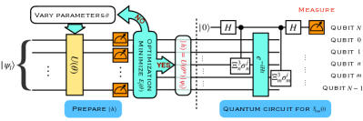
Figure 1: Quantum circuit for the calculation of PDFs. On the left-hand side of the dashed line is the circuit for hadronic state preparation, while the right-hand side is for the correlation function.

1. Hadronic state preparation. Simulating hadronic states for a generic quantum field system on a quantum computer typically involves preparing excited states with specified quantum numbers. For this purpose, we develop a framework of the quantum-number-resolving VQE. The quantum circuit for hadronic state preparation is illustrated on the left-hand side of the dashed line shown in Fig. 1 and involves two steps.

First of all, we construct trial hadronic states for the $k$th excited state with a set of quantum numbers $l$ as

$$\ket{\psi_{lk}(\theta)}=U(\theta)\ket{\psi_{lk}}_{\rm ref}\,,$$ (7)

where $\ket{\psi_{lk}}_{\rm ref}$ is an input reference state and $U(\theta)$ encodes a set of symmetry-preserving unitary operators with parameters $\theta$.

The input states $\ket{\psi_{l}}_{\rm ref}$ with discrete quantum numbers—such as the charge, the baryon number, and the spin—can be realized as computational bases specified by those quantum numbers. In addition, to preserve the spatial symmetries, the input state of a given momentum will be represented by a superposition of the computational bases, and its preparation is similar to those of the Dicke states B_rtschi_2019 . Specifically for the PDFs, zero momentum is chosen for the trial state.

The symmetry-preserving unitary evolution $U(\theta)$ is constructed using the quantum alternating operator ansatz (QAOA farhi2014quantum , also related to the Hamiltonian variational ansatz wiersema-PRXQuantum2020 ). To retain the representation power yet preserve the quantum numbers for the ansatz, the Hamiltonian is divided as $H=H_{1}+H_{2}+\cdots+H_{n}$ with $n\geq 2$, where every $H_{i}$ inherits the symmetries of $H$ and $[H_{i},H_{i+1}]\not=0$. The $U(\theta)$ then consists of multiple layers, with each layer constructed by alternately evolving $H_{j}$ with parametrized time duration $\theta_{ij}$,

$$U(\theta)\equiv\prod_{i=1}^{p}\prod_{j=1}^{n}\exp(i\,\theta_{ij}H_{j})\,.$$ (8)

Here $p$ is the number of layers, and trial states with larger $p$ and $n$ represent the objective hadronic state more faithfully. By construction, the operator $U(\theta)$ will evolve the initial state $\ket{\psi_{lk}}_{\rm ref}$ into $\ket{\psi_{lk}(\theta)}$ due to the noncommutativity of two consecutive evolutions $\exp(i\theta_{ij}H_{j})$ and $\exp(i\theta_{ij-1}H_{j-1})$, while preserving the quantum numbers $l$.

The second step is the optimization for hadronic states, which can be realized by minimizing the cost function constructed out of a weighted combination of energy expectations nakanishi_19 ,

$$E_{l}(\theta)=\sum_{i=1}^{k}w_{li}\bra{\psi_{li}(\theta)}H\ket{\psi_{li}(\theta)}\,,$$ (9)

for $k$ excited states with the same $l$ to determine the optimized parameter set $\theta^{\ast}$. Here we require $w_{l1}>w_{l2}>\cdots>w_{lk}$. The $k$th excited hadron state $\ket{h}$ is then prepared as $\ket{h}=U(\theta^{\ast})\ket{\psi_{lk}}_{\rm ref}$.

Returning to the specific $1+1$D NJL model we are discussing, the mapping onto a quantum computer has been carried out in the previous section. The Hamiltonian is found to take the form

$$H=H_{1}+H_{2}+H_{3}+H_{4}\,,$$ (10)

where

$$H_{1}= \sum_{\alpha}\sum_{n={\rm even}}^{\frac{N}{2}-1}\frac{1}{4}\left(\sigma_{\alpha,n}^{1}\sigma_{\alpha,n+1}^{2}-\sigma_{\alpha,n}^{2}\sigma_{\alpha,n+1}^{1}\right)\,,$$

$$H_{2}= \sum_{\alpha}\sum_{n={\rm even}}^{\frac{N}{2}-1}\,\frac{g}{2}\,\sigma_{\alpha,n}^{3}\sigma_{\alpha,n+1}^{3}+\sum_{\alpha,\beta}H_{\rm int,\alpha\beta}\,,$$

$$H_{3}= H_{1}(n={\rm even}\to n={\rm odd})$$

$$+\frac{1}{4}\sum_{\alpha}\tilde{\sigma}^{3}_{\alpha,\frac{N}{2}}\left(\sigma_{\alpha,\frac{N}{2}-1}^{2}\sigma_{\alpha,0}^{1}-\sigma_{\alpha,\frac{N}{2}-1}^{1}\sigma_{\alpha,0}^{2}\right)\,,$$

$$H_{4}= \sum_{\alpha}\sum_{n=0}^{\frac{N}{2}-1}\frac{m_{\alpha}}{2}(-1)^{n}(I-\sigma_{\alpha,n}^{3})-\frac{g}{2}(I-\sigma_{\alpha,n}^{3})\,,$$ (11)

where the second line of $H_{3}$ comes from the periodic boundary condition, and the interaction between different quark flavors $\alpha$ and $\beta$ is given by

$$H_{{\rm int},\alpha\beta} =-\frac{g}{2}\sum_{n={\rm even}}^{\frac{N}{2}-1}\sigma_{\alpha,n}^{3}\sigma_{\beta,n}^{3}+\sigma_{\alpha,n+1}^{3}\sigma_{\beta,n+1}^{3}$$

$$\quad\quad-\sigma_{\alpha,n+1}^{3}\sigma_{\beta,n}^{3}-\sigma_{\alpha,n}^{3}\sigma_{\beta,n+1}^{3}\,.$$ (12)

Here, $H_{2}$ and $H_{4}$ are diagonal. It is also straightforward to check that $H_{i}$ satisfies the condition $[H_{i},H_{i+1}]\neq 0$ and meanwhile inherits the symmetries of $H$, following from $[Q^{i},H_{i}]=0$ and $[T,H_{i}]=0$ for $i=1,\cdots,4$. Note that $T$ is the even-lattice translation operator, acting as $T^{-1}\sigma_{n}^{i}T=\sigma_{n+2}^{i}$, and $Q^{i}$ include the flavors and the electromagnetic charge. It is noted that the mass $m_{\alpha}$ and the coupling constant $g$ can be absorbed into the parameter set $\theta$.

To prepare the input reference states for QAOA, we follow the strategy introduced before. For instance, to construct a zero-charge hadronic state with the lowest mass out of the $1$-flavor NJL model (the $1$st excitation state with respect to the vacuum $\Omega$), the input states can be chosen as

$$\ket{\psi_{\Omega,1}}_{\rm ref}= \ket{010101\dots 01}\,,$$

$$\ket{\psi_{\Omega,2}}_{\rm ref}= \frac{1}{\sqrt{N/2}}\left(\ket{1001,\dots,01}+\ket{0110,\dots,01}\right.$$

$$\left.+\dots+\ket{0101,\dots,10}\right)\,,$$ (13)

from which it immediately follows that $Q\ket{\psi_{\Omega,1}}_{\rm ref}=Q\ket{\psi_{\Omega,2}}_{\rm ref}$, where $Q=\frac{e_{q}}{2}\sum_{n}(I-\sigma_{n}^{3})$ is the electromagnetic charge operator.

Then we apply the QAOA to evolve the reference states to the objective vacuum and the hadronic state by minimizing the cost function $E_{\Omega}(\theta)$. Within $E_{\Omega}(\theta)$, we can choose, for instance, $w_{\Omega,1}=1$ and $w_{\Omega,2}=0.5$. For the cases with more flavors, the hadronic states can be prepared in a similar way.

2. Dynamical correlation function. With the hadronic state at hand, to obtain the PDFs, we implement the quantum circuit illustrated on the right-hand side of the dashed line in Fig. 1, following the standard technique in Ref. PhysRevLett.113.020505 , to evaluate the $2$-point dynamical correlation function,

$$S_{mn}(t)=\bra{h}e^{iHt}\Xi^{3}_{m}\sigma^{i}_{m}e^{-iHt}\Xi^{3}_{n}\sigma^{j}_{n}\ket{h}\,,$$ (14)

with $i(j)=1,2$. The $D(z)$ in Eq. (6) can then be written as a sum of such correlation functions (see Supplemental Materials supp ).

The quantum algorithm encodes the information of the dynamical correlation function into an ancillary qubit which controls and probes the system of the simulated hadron. More specifically, one inserts an evolution $e^{-iHt}$ between two $\Xi^{3}_{n}\sigma^{j}_{n}$ and $\Xi^{3}_{m}\sigma^{i}_{m}$ operations controlled by the ancilla and then measures the ancilla on the $\sigma^{1}$ ($\sigma^{2}$) basis to get the real (imaginary) part of the correlation function. Assuming that the probability of getting $\ket{0}$ out of the ancilla is $p_{mn}(t)$ for a given $m$ and $n$ in the circuit, both the real and the imaginary parts of the correlation function can be found immediately through PhysRevLett.113.020505

$$S_{mn}(t)=p_{mn}(t)-\frac{1}{2}\,,$$ (15)

hence finishing the calculation of the PDFs. Here we also calculate the vacuum propagator by replacing $\ket{h}$ with the vacuum $\ket{\Omega}$ in Eq. (14), and we follow Collins:2011zzd ; Jia:2018qee to remove the disconnected contributions.

We now estimate the time complexity of our quantum approach. The depth of the parametric quantum circuit for preparing the hadron state with the QAOA ansatz is expected to be $O(N)$ wiersema-PRXQuantum2020 . Since optimization with such ansatz is believed to be almost trapped-free and quick to converge wiersema-PRXQuantum2020 , we could estimate the complexity of the state preparation as $O(N)$. Extracting the PDFs involves a series of measurements of the dynamical correlation function $S_{mn}(t)$ at $t=1,2,\cdots,N/2$, with each $t=n$ taking a cost of $O(n^{2}/\varepsilon)$ under a desired precision $\varepsilon$. The cost mostly comes from decomposing the real-time evolution $e^{iHt}$ with the Trotter formula nielsen_chuang_2010 . From the above analysis, the total time complexity for calculating the PDFs is $O(N^{3}/\varepsilon)$.

The polynomial scaling with the number of qubits—and, more notably, the ability to attain real-time light-cone evolution—clearly shows a quantum advantage of calculating hadron PDFs on a quantum computer. Although justified only with a 1+1D quantum system, the quantum advantage could still hold for generic quantum systems in higher space-time dimensions and with gauge fields, if one can map the non-Abelian gauge field onto qubits in an efficient way Brower:1997ha ; Banerjee:2012xg ; Stryker:2020sap . Remarkably, even with the presence of a Wilson line in the correlator of Eq. (Partonic collinear structure by quantum computing) due to the gauge field, PDFs can still be efficiently evaluated on a quantum computer (see Supplemental Material supp ).

Results.—Considering the current limitations of using real quantum devices, we present results using a classical simulation of the quantum circuit in Fig. 1. The simulation is performed on a desktop workstation with $16$ cores, using the open source packages QuSpin quspin and projectQ Steiger2018projectqopensource . For the time being, we use $N=12$ or $18$ qubits and set $a=1$ for the lattice spacing, which is sufficient to demonstrate the feasibility of the proposed quantum algorithm. In reality, the lattice spacing $a$ and quark mass $m$ will be fixed by the values of the coupling constant $g$ and relevant physical quantities such as hadron masses.

To verify the simulation, we first measure the mass of the lowest-lying $ud$-like hadron $M_{h}=\bra{h}H\ket{h}$ with respect to the vacuum energy $\bra{\Omega}H\ket{\Omega}$, in the NJL model with 2 flavors. We compare the result $M_{h,{\rm QC}}$ with $M_{h,{\rm NUM}}$, where the subscripts ${\rm QC}$ and ${\rm NUM}$ stand for the results obtained by quantum computing and exact diagonalization (ED), respectively. For simplicity, we set $ma=0.2$ for both flavors. The comparison is shown in Table 1. The differences between these two approaches are at the percent level, thus justifying the setups. It is also interesting to note that for small quark mass, the dominant contribution to the hadron mass comes from the interactions rather than the quark masses. This is consistent with the picture that QCD dynamics generates the majority of the hadron mass Ji:1994av ; Accardi:2012qut ; Anderle:2021wcy ; Yang:2018nqn ; Ji:2021mtz .

$g$	0.2	0.4	0.6	0.8	1.0
$M_{h,{\rm QC}}a$	1.002	1.810	2.674	3.534	4.352
$M_{h,{\rm NUM}}a$	1.001	1.801	2.659	3.509	4.342

Table 1: Calculated hadron mass as a function of $g$ with $N=12$.

We also test the results with a heavier quark mass $ma=0.8$ in the $1$-flavor model. In that case the hadron mass is dominated by the quark masses $2m$ from the hadron valence components. This is consistent with the expectation on the similarity with the mass configuration of a heavy quarkonium.

Now we present the quark PDF of the lowest-lying zero-charge hadron in the $1$-flavor NJL model, which mimics the quark PDFs for $\pi^{0}$. Considering the reliability of the results and tolerable computing time, we use $N=18$ and fix the quark mass $ma=0.8$. We show distributions in both position space $D(z)$ and momentum space $f_{q}(x)$.

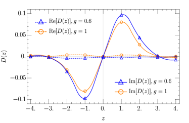
Figure 2: Real (dashed lines) and imaginary parts (solid lines) of the quark field correlation function in position space. The discrete points are the lattice data, and the lines are from interpolations.

In Fig. 2, we plot the imaginary and real parts of $D(z)$. We show results for both $g=0.6$ and $g=1.0$. In the plot, the discrete open markers are from the direct quantum computations. The real part shown in Fig. 2 is compatible with zero, implying that $f_{q}(x)=-f_{q}(-x)$. Since $f_{\bar{q}}(x)=-f_{q}(-x)$ holds after subtraction of the disconnected part Collins:2011zzd , we have $f_{q}(x)=f_{\bar{q}}(x)$, which is consistent with our expectation for one-flavor PDFs. To obtain the PDF $f_{q}(x)$, a continuous Fourier transformation of $D(z)$ will be performed. For this purpose, we interpolate the discrete results, as shown by the lines in Fig. 2.

The results for the PDF are given in Fig. 3. We show $f_{q}(x)$ from both the quantum computations (in open markers) and the ED to the NJL model (in solid lines). A perfect agreement between these two distinct approaches is observed. In Fig. 3, the error bars/bands illustrate the estimated uncertainties due to different ways of interpolations in $D(z)$. The nonvanishing but suppressed contributions in the nonphysical region $x>1$ are partly due to the finite volume effect, which is also commonly seen in lattice calculations (see, for instance, Ref. Ishikawa:2019flg ). It is expected to be further suppressed when more lattice sites and hence a larger volume are used. Here we note that the renormalization and calibration of input parameters, such as the lattice spacing $a$ and the quark mass $m$, for the NJL model are not yet considered in this initial exploration, whose focus is the practicability of a generic quantum algorithm for PDF evaluations. A discussion of the renormalization procedure and specific tuning of input parameters to physical quantities for the NJL model and QCD will be left for future publications. Nevertheless, we observe the expected peak around $x=0.5$, and the shapes shown in Fig. 3 are in qualitative agreement with the calculated $f_{q}(x)$ in two-dimensional QCD Jia:2018qee and the extracted pion PDFs from the JAM Collaboration Barry:2021osv .

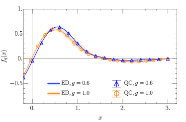
Figure 3: Quark PDF from quantum computing (open markers) and ED (solid lines). The error bars/bands arise from the estimated uncertainties due to different interpolation methods.

Summary.—In this work, we presented the first direct simulation of the hadron partonic structure on a quantum computer. To realize such a calculation, we proposed a systematic quantum algorithm for preparing hadronic states using the quantum-number-resolving VQE, and we designed the quantum circuit to perform the real-time evolution of the lightlike correlators. As a proof of concept, we demonstrated the viability of the quantum algorithm by calculating the PDF in the $1+1$ dimensional NJL model. Our simulation results using only $18$ qubits agree with the ED to the discretized NJL model. Our results manifest the quantum advantage over the classical Euclidean lattice methodology in resolving the intrinsic difficulties of simulating real-time dynamics. Our exploratory study suggests the possible future capability of studying realistic hadron structures on current and/or near-term quantum computers. Lastly, we point out that the proposed quantum computing framework for preparing the hadronic states and measuring the dynamical correlation functions is generally applicable. Its extension to many applications in high energy particle and nuclear physics is expected, such as calculations of scattering processes and parton showers Bepari:2020xqi ; Bauer:2019qxa ; Bauer:2021gup , the proton spin configurations, the 3D structure of a nucleon, as well as the fundamental jet transport properties Barata:2021yri and the associated dynamics Cohen:2021imf ; deJong:2020tvx of quark-gluon plasma.

- (1) H.-W. Lin et al., Prog. Part. Nucl. Phys. 100, 107 (2018).
- (2) J. Gao, L. Harland-Lang, and J. Rojo, Phys. Rep. 742, 1 (2018).
- (3) J. C. Collins, D. E. Soper, and G. F. Sterman, Adv. Ser. Direct. High Energy Phys. 5, 1 (1989).
- (4) T.-J. Hou et al., Phys. Rev. D 103, 014013 (2021).
- (5) L. A. Harland-Lang, A. D. Martin, P. Motylinski, and R. S. Thorne, Eur. Phys. J. C 75, 204 (2015).
- (6) R. D. Ball et al., (NNPDF collaboration), Eur. Phys. J. C 77, 663 (2017).
- (7) S. Alekhin, J. Blümlein, S. Moch, and R. Placakyte, Phys. Rev. D 96, 014011 (2017).
- (8) H. Abramowicz et al., (H1 and ZEUS Collaboration), Eur. Phys. J. C 75, 580 (2015).
- (9) J. J. Ethier, N. Sato, and W. Melnitchouk, Phys. Rev. Lett. 119, 132001 (2017).
- (10) P. C. Barry, N. Sato, W. Melnitchouk, and C.-R. Ji, Phys. Rev. Lett. 121, 152001 (2018).
- (11) X. Ji, Phys. Rev. Lett. 110, 262002 (2013).
- (12) X. Ji, Sci. China Phys. Mech. Astron. 57, 1407 (2014).
- (13) Y.-Q. Ma and J.-W. Qiu, Phys. Rev. D 98, 074021 (2018).
- (14) Y.-Q. Ma and J.-W. Qiu, Phys. Rev. Lett. 120, 022003 (2018).
- (15) A. V. Radyushkin, Phys. Rev. D 96, 034025 (2017).
- (16) K. Orginos, A. Radyushkin, J. Karpie, and S. Zafeiropoulos, Phys. Rev. D 96, 094503 (2017).
- (17) J. Liang, T. Draper, K.-F. Liu, A. Rothkopf, and Y.-B. Yang, (XQCD Collaboration), Phys. Rev. D 101, 114503 (2020).
- (18) A. J. Chambers et al., Phys. Rev. Lett. 118, 242001 (2017).
- (19) R. S. Sufian et al., Phys. Rev. D 99, 074507 (2019).
- (20) T. Izubuchi et al., Phys. Rev. D 100, 034516 (2019).
- (21) H.-W. Lin, J.-W. Chen, Z. Fan, J.-H. Zhang, and R. Zhang, Phys. Rev. D 103, 014516 (2021).
- (22) B. U. Musch, P. Hagler, M. Engelhardt, J. W. Negele, and A. Schafer, Phys. Rev. D 85, 094510 (2012).
- (23) W. Detmold, W. Melnitchouk, J. W. Negele, D. B. Renner, and A. W. Thomas, Phys. Rev. Lett. 87, 172001 (2001).
- (24) P. Hagler et al., (LHPC Collaboration), Phys. Rev. D 77, 094502 (2008).
- (25) C. Alexandrou et al., J. High Energy Phys. 06, 068 (2015).
- (26) C. Alexandrou et al., Phys. Rev. D 101, 094513 (2020).
- (27) F. Arute et al., Nature (London) 574, 505 (2019).
- (28) Y. Alexeev et al., PRX Quantum. 2, 017001 (2021).
- (29) M. R. Dietrich et al., arXiv:1903.05453.
- (30) D.-B. Zhang, H. Xing, H. Yan, E. Wang, and S.-L. Zhu, Chin. Phys. B 30, 020306 (2021).
- (31) H. Lamm, S. Lawrence, and Y. Yamauchi, (NuQS Collaboration), Phys. Rev. Research 2, 013272 (2020).
- (32) M. G. Echevarria, I. L. Egusquiza, E. Rico, and G. Schnell, Phys. Rev. D 104, 014512 (2021).
- (33) N. Mueller, A. Tarasov, and R. Venugopalan, Phys. Rev. D 102, 016007 (2020).
- (34) A. Pérez-Salinas, J. Cruz-Martinez, A. A. Alhajri, and S. Carrazza, Phys. Rev. D 103, 034027 (2021).
- (35) Y. Nambu and G. Jona-Lasinio, Phys. Rev. 122, 345 (1961).
- (36) Y. Nambu and G. Jona-Lasinio, Phys. Rev. 124, 246 (1961).
- (37) D. J. Gross and A. Neveu, Phys. Rev. D 10, 3235 (1974).
- (38) C. V. Christov et al., Prog. Part. Nucl. Phys. 37, 91 (1996).
- (39) S. Backens, A. Shnirman, and Y. Makhlin, Sci. Rep. 9 (2019).
- (40) A. Bärtschi and S. Eidenbenz, Lect. Notes Comput. Sci. , 126 (2019).
- (41) E. Farhi, J. Goldstone, and S. Gutmann, 2014, arXiv:1411.4028.
- (42) R. Wiersema et al., PRX Quantum 1, 020319 (2020).
- (43) K. M. Nakanishi, K. Mitarai, and K. Fujii, Phys. Rev. Research 1, 033062 (2019).
- (44) J. S. Pedernales, R. Di Candia, I. L. Egusquiza, J. Casanova, and E. Solano, Phys. Rev. Lett. 113, 020505 (2014).
- (45) See supplemental material at ”http://link.aps.org/supplemental/10.1103/PhysRevD.105.L111502” for details of preparing the reference states and evaluating the dynamical correlation function. moreover, an extension of the quantum computing framework for pdfs with wilson lines is elaborated.
- (46) J. Collins, Foundations of Perturbative QCD (Cambridge University Press, Cambridge, England, 2013).
- (47) Y. Jia, S. Liang, X. Xiong, and R. Yu, Phys. Rev. D 98, 054011 (2018).
- (48) M. A. Nielsen and I. L. Chuang, Quantum Computation and Quantum Information: 10th Anniversary Edition (Cambridge University Press, Cambridge, England, 2010).
- (49) R. Brower, S. Chandrasekharan, and U. J. Wiese, Phys. Rev. D 60, 094502 (1999).
- (50) D. Banerjee et al., Phys. Rev. Lett. 110, 125303 (2013).
- (51) J. Stryker, Compiling quantum gauge theories for quantum computation, PhD thesis, University Washington, Seattle (main), 2020.
- (52) P. Weinberg and M. Bukov, SciPost Phys. 2, 003 (2017).
- (53) D. S. Steiger, T. Häner, and M. Troyer, Quantum 2, 49 (2018).
- (54) X.-D. Ji, Phys. Rev. Lett. 74, 1071 (1995).
- (55) A. Accardi et al., Eur. Phys. J. A 52, 268 (2016).
- (56) D. P. Anderle et al., Front. Phys. (Beijing) 16, 64701 (2021).
- (57) Y.-B. Yang et al., Phys. Rev. Lett. 121, 212001 (2018).
- (58) X. Ji, Front. Phys. (Beijing) 16, 64601 (2021).
- (59) T. Ishikawa et al., Sci. China Phys. Mech. Astron. 62, 991021 (2019).
- (60) P. C. Barry, C.-R. Ji, N. Sato, and W. Melnitchouk, [Jefferson Lab Angular Momentum (JAM)], Phys. Rev. Lett. 127, 232001 (2021).
- (61) K. Bepari, S. Malik, M. Spannowsky, and S. Williams, Phys. Rev. D 103, 076020 (2021).
- (62) C. W. Bauer, W. A. de Jong, B. Nachman, and D. Provasoli, Phys. Rev. Lett. 126, 062001 (2021).
- (63) C. W. Bauer, M. Freytsis, and B. Nachman, Phys. Rev. Lett. 127, 212001 (2021).
- (64) J. a. Barata and C. A. Salgado, Eur. Phys. J. C 81, 862 (2021).
- (65) T. D. Cohen, H. Lamm, S. Lawrence, and Y. Yamauchi, (NuQS Collaboration), Phys. Rev. D 104, 094514 (2021).
- (66) W. A. De Jong et al., Phys. Rev. D 104, 051501 (2021).