Simulating relic gravitational waves from inflationary magnetogenesis

Abstract

We present three-dimensional direct numerical simulations of the production of magnetic fields and gravitational waves (GWs) in the early Universe during a low energy scale matter-dominated post-inflationary reheating era, and during the early subsequent radiative era, which is strongly turbulent. The parameters of the model are determined such that it avoids a number of known physical problems and produces magnetic energy densities between 0.03% and 0.5% of the critical energy density at the end of reheating. During the subsequent development of a turbulent magnetohydrodynamic cascade, magnetic fields and GWs develop a spectrum that extends to higher frequencies in the millihertz (nanohertz) range for models with reheating temperatures of around $100\,{\rm GeV}$ ($150\,{\rm MeV}$) at the beginning of the radiation-dominated era. However, even though the turbulent cascade is fully developed, the GW spectrum shows a sharp drop for frequencies above the peak value. This suggests that the turbulence is less efficient in driving GWs than previously thought. The peaks of the resulting GW spectra may well be in the range accessible to space interferometers, pulsar timing arrays, and other facilities.

1 Introduction

During the past few years, numerical simulations of gravitational wave (GW) generation from early Universe turbulence have become an essential tool in predicting the stochastic background that the Laser Interferometer Space Antenna (LISA; see, e.g., Amaro-Seoane et al., 2017) and other space interferometers (e.g., Taiji Scientific Collaboration et al., 2021) might see in the future. Most of the existing predictions are based on analytical models (Dolgov et al., 2002; Kosowsky et al., 2002; Caprini & Durrer, 2006; Niksa et al., 2018), which tend to make simplifying assumptions about the nature of turbulent wave generation; see Caprini et al. (2016) and Caprini & Figueroa (2018) for recent reviews emphasizing the feasibility and prospects of observing such relic GWs.

A particularly popular source of turbulence in the early Universe is the electroweak phase transition. Hindmarsh et al. (2015, 2017) have produced numerical simulations of GW generation by assuming a first order phase transition (Kosowsky et al., 1992; Kamionkowski et al., 1994; Nicolis, 2004; Ellis et al., 2019, 2020). Even if the phase transition is not a first order one, as initially assumed, it is still possible to produce primordial turbulence from magnetic fields that could be generated during various epochs in the early Universe (see, e.g., Cornwall, 1997; Joyce & Shaposhnikov, 1997; Bhatt & Pandey, 2016; Miniati et al., 2018). The existence of large-scale magnetic fields in the early universe is motivated by indirect evidence of their presence in the intergalactic regime from the non-detection of GeV photons in blazar observations (Neronov & Vovk, 2010; Taylor et al., 2011; Tavecchio et al., 2011; Ackermann et al., 2018; Archambault et al., 2017).

Both analytical considerations (Dolgov et al., 2002; Kosowsky et al., 2002; Gogoberidze et al., 2007; Kahniashvili et al., 2008) and numerical simulations (Roper Pol et al., 2020b) have demonstrated that there can be a direct correspondence between the turbulence spectrum and the resulting GW spectrum. An important additional property of GWs might be their circular polarization, which could be caused by helical turbulence (Kahniashvili et al., 2005) or by helical magnetic fields (Namba et al., 2016; Niksa et al., 2018; Anand et al., 2019; Sharma et al., 2020; Okano & Fujita, 2021). Again, numerical simulations have confirmed the direct correspondence between the fractional helicity of magnetic fields and the resulting circular polarization of GWs (Kahniashvili et al., 2021).

Magnetogenesis during quantum chromodynamic (QCD) phase transitions (Quashnock et al., 1989; Sigl et al., 1997; Tevzadze et al., 2012) provide another possible avenue for GW generation at low frequencies in the nanohertz range (Kahniashvili et al., 2010; Neronov et al., 2021). If the characteristic scale of QCD turbulence is a significant fraction of the Hubble horizon at that time, as suggested by some models (e.g., Kisslinger et al., 2005), the resulting GW spectrum could show a marked drop in the spectral energy density for frequencies above the value typical of the turbulent driving scale (Brandenburg et al., 2021a). This result has been obtained by assuming the turbulence to be driven by a monochromatic forcing function. However, it remains unclear how sensitive such results are to the assumption of an artificially adopted forcing function. For this reason, it is essential to include the magnetogenesis mechanism in the actual simulations of GW production, without using any artificial forcing. One such mechanism is the dynamo effect associated with the chirality of fermions (Joyce & Shaposhnikov, 1997), which is referred to as the chiral magnetic effect (Vilenkin, 1980). Numerical simulations of the resulting GW generation predict that their power depends on the speeds of magnetic field generation and saturation (Brandenburg et al., 2021c). However, this model suffers from the difficulty that the typical length scale associated with the chiral magnetic effect is very short. For this reason, we focus here on magnetogenesis during inflation. It is traditionally expected to produce a large-scale magnetic field (Ratra, 1992; Martin & Yokoyama, 2008; Subramanian, 2010; Kahniashvili et al., 2017; Fujita & Durrer, 2019). However, as we discuss next, it is unclear how to properly model GW production for such a magnetic field.

Earlier approaches modeled the process of GW production from magnetic fields by assuming a magnetic field to be given; see the models ini1–ini3 in Roper Pol et al. (2020b) for such examples. However, this corresponds to switching on a magnetic field abruptly at a particular time. Therefore, the process of switching on a magnetic field with a given spectrum played a decisive role in the resulting GW energy and strain. The result would be different if the field was gradually being produced by some magnetogenesis mechanism. Including a suitable magnetogenesis model is what will be presented in this paper. This will then also allow us to quantify the resulting differences. We can therefore demonstrate what difference it would make when we just switched on the magnetic field from our magnetogenesis simulation without including the corresponding GW generation until that time.

A popular model of inflationary magnetogenesis is that of Ratra (1992), where electromagnetic fields originate from quantum fluctuations (Fischler et al., 1985) that are being amplified during inflation owing to the breaking of conformal invariance (Turner & Widrow, 1988; Dolgov, 1993). This is achieved by a suitable coupling of the inflaton field to the electromagnetic field through a function $f$ leading to a term of the form $f^{2}F^{\mu\nu}F_{\mu\nu}$ in the Lagrangian density, where $F_{\mu\nu}$ is the Faraday tensor. One usually assumes $f$ to be proportional to some power $\alpha$ of the scale factor $a$ (Bamba & Sasaki, 2007; Martin & Yokoyama, 2008; Subramanian, 2010), i.e.,

$$f(a)\propto a^{\alpha}.$$ (1)

Of particular interest are scale-invariant magnetic fields, which can be obtained for $\alpha=2$ and $-3$ assuming constant expansion rate during inflation. Although the strength of the resulting magnetic field in such models may well be of astrophysical interest, they suffered from three major shortcomings. (i) In the case $\alpha=2$, the function $f$ increases from a certain initial value to a very large value at the end of inflation. Demanding standard electromagnetism at the end of inflation requires $f=1$, but this would imply a very small value of $f$ at the beginning of inflation. This results in very large values of the effective electric charge, defined as $e_{\rm eff}=e/f^{2}$ (Subramanian, 2010; Kobayashi, 2014), where $e$ is the standard elementary charge. Therefore, there will be a very large coupling between the electromagnetic and charged fields at the beginning of inflation. For this reason, this theory would be in the nonperturbative regime and would therefore not be reliable. This is known as the strong coupling problem (Demozzi et al., 2009). (ii) In the other case, where $\alpha=-3$, the electric energy density diverges and may overshoot the background energy density during inflation. This problem is known as the backreaction problem (Demozzi et al., 2009). (iii) The production of charged particles in the presence of strong electric fields due to the Schwinger effect can lead to a premature increase in the electric conductivity, which shorts the electric field and prevents further magnetic field growth; see Kobayashi & Afshordi (2014). This problem also applies to models that solve the backreaction problem by choosing a low energy scale inflation (Ferreira et al., 2013). Such a problem could be avoided if charged particles get sufficiently large masses by some mechanism in the early Universe, as suggested by Kobayashi & Sloth (2019).

The Sharma et al. (2017, 2018) model addresses the three problems by constraining the form of $f(a)$ such that $\alpha=2$ during inflation, starting at an initial value of unity, thereby solving the strong coupling problem, and to obey

$$f(a)\propto a^{-\beta}$$ (2)

during a post-inflationary era, which is assumed to be matter dominated. The exponent $\beta>0$ is calculated for a given reheating temperature. By choosing the reheating temperature to be at the electroweak scale of $100\,{\rm GeV}$ and the total electromagnetic energy density to be $1\%$ of the background energy density, the number of $e$-folds of the scale factor during inflation, $N$, and during reheating, $N_{\rm r}$, are found to be 34 and 9.3, respectively. To arrive at standard electrodynamics with $f=1$ at the end of reheating, we require $\alpha N=\beta N_{\rm r}$, and therefore $\beta=\alpha N/N_{\rm r}=7.3$. Alternatively, following Sharma et al. (2020) and Sharma (2021), we can consider the case where the reheating temperature is at the QCD energy scale of $150\,{\rm MeV}$, for which one finds $N=36$, $N_{\rm r}=28$, and therefore $\beta=2.7$; see Appendix A for the details.

A similar model for helical magnetic field generation and polarized GWs was recently considered by Sharma et al. (2020) and Okano & Fujita (2021). These studies are based on earlier work of Durrer et al. (2011), Caprini & Sorbo (2014), Fujita et al. (2015), Sharma et al. (2018), and Fujita & Durrer (2019). However, the numerical consideration of such models is beyond the scope of the present work and is the subject of a separate paper (Brandenburg et al., 2021d).

Here, we adopt the aforementioned magnetogenesis model of Sharma et al. (2017) to compute both electromagnetic fields and GWs resulting from the electromagnetic stress during the late reheating phase, when the conductivity is still negligible, and during the early radiation-dominated phase when the conductivity is high and the laws of magnetohydrodynamics (MHD) are applicable. In the first step, magnetic fields and GWs exist only on very large length scales. The significance of the second step is therefore to produce magnetic fields and GWs at smaller length scales through turbulence that is being driven by the Lorentz force from electric currents once the conductivity is high. By making simplifying assumptions, Sharma et al. (2020) have already considered this case, but avoiding the restrictions resulting from these assumptions requires self-consistently computed turbulence, which can only be done numerically.

2 The model

We consider a periodic domain of size $L^{3}$. The smallest wavenumber is then $2\pi/L\equiv k_{1}$. In this work, we use cubic domains with $n=512$ or $1024$ mesh points in each direction with $k_{1}=1$, so the Nyquist wavenumber, $k_{\rm Ny}=k_{1}n/2$, is either $256$ or $512$. We adopt a spatially flat Friedmann–Lemaître–Robertson–Walker metric. Throughout this paper, we use conformal time $\eta=\int{\rm d}{}t/a(t)$, where $t$ is the physical time, and work with comoving variables that are scaled by the appropriate powers of $a$. In particular, the MHD equations then become equal to the MHD equations in a non-expanding universe (Brandenburg et al., 1996). Our comoving variables therefore describe the departures from the expansion of the Universe. The speed of light is always set to unity and the Lorentz–Heaviside unit system is used for the Maxwell equations. We also set the density at the beginning of the radiation-dominated era to unity. This also implies that the mean radiation energy density is unity and therefore the magnetic energy densities quoted below are automatically the fractional magnetic energy densities with respect to the radiative energy density.

As was suggested in the introduction, we perform the simulations in two separate steps. In step I, during the end of reheating, we solve the Maxwell equations with zero conductivity, but, owing to the breaking of conformal invariance, with a nonvanishing $f^{\prime\prime}/f$ term, where primes denote derivatives with respect to $\eta$. Similarly, in the GW equation, the $a^{\prime\prime}/a$ term is nonvanishing. In step II, we assume a rapid transition into the radiation-dominated era, where the electric field can be neglected and we thus solve the MHD equations. Owing to finite conductivity, electric currents can flow and drive fluid motions through the Lorentz force, which leads to additional induction and magnetic field amplification at small length scales. In that case, $f=1$ and $a\propto\eta$ grows linearly, so $f^{\prime\prime}/f=a^{\prime\prime}/a=0$.

Following Roper Pol et al. (2020b), we scale the conformal time at the beginning of the radiative era to unity, i.e., $\eta=1$. We simulate the last phase $\eta_{\rm ini}\leq\eta\leq 1$ of the reheating interval, where the scale factor is taken to be $a=(\eta+1)^{2}/4$ so as to match $a=1$ at $\eta=1$ (Sharma et al., 2017). In practice, we consider as the initial value of the conformal time $\eta_{\rm ini}=-0.9$, corresponding to an initial scale factor of $a_{\rm ini}=1/400$. Thus, we have

$$\frac{a^{\prime\prime}}{a}=\frac{2}{(\eta+1)^{2}}\quad\mbox{and}\quad\frac{f^{\prime\prime}}{f}=\frac{2\beta(2\beta+1)}{(\eta+1)^{2}}.$$ (3)

In step I, we solve the following equations for variables in Fourier space, denoted by tildae on the scaled magnetic vector potential ${\mathbfcal{A}}$ and the strains $h_{+}$ and $h_{\times}$ for the two linear polarizations modes:

$$\tilde{\mathbfcal{A}}^{\prime\prime}+\left(\mathbf{k}^{2}-\frac{f^{\prime\prime}}{f}\right)\tilde{\mathbfcal{A}}=0,$$ (4)

$$\tilde{h}_{+/\times}^{\prime\prime}+\left(\mathbf{k}^{2}-\frac{a^{\prime\prime}}{a}\right)\tilde{h}_{+/\times}={6\over a}\,\tilde{T}_{+/\times}.$$ (5)

Here, $\tilde{\mathbfcal{A}}=f\tilde{\mathbf{A}}$, where $\tilde{\mathbf{A}}$ is the magnetic vector potential and $\tilde{T}_{+/\times}(\eta,\mathbf{k})={\sf e}_{+/\times}^{ij}\tilde{\sf T}_{ij}(\eta,\mathbf{k})$ are the $+$ and $\times$ polarizations of the traceless-transverse projected stress in Fourier space, where $\tilde{\sf T}_{ij}(\eta,\mathbf{k})=\int{{\sf T}}_{ij}(\eta,\mathbf{x})\,e^{-{\rm i}\mathbf{k}\cdot\mathbf{x}}{\rm d}{}^{3}\mathbf{x}$ is the Fourier transformation of the electromagnetic stress, given in real space by

$${{\sf T}}_{ij}=f^{2}\,(B_{i}B_{j}+E_{i}E_{j}).$$ (6)

Here, $\mathbf{E}=-\partial\mathbf{A}/\partial\eta$ and $\mathbf{B}={\mathbf{\nabla}}\times\mathbf{A}$ are computed through inverse Fourier transformation, $\mathbf{E}(\eta,\mathbf{x})=\int\tilde{\mathbf{E}}(\eta,\mathbf{k})\,e^{{\rm i}\mathbf{k}\cdot\mathbf{x}}{\rm d}{}^{3}\mathbf{k}/(2\pi)^{3}$, and likewise for $\tilde{\mathbf{B}}(\eta,\mathbf{k})$, which is given by $\tilde{\mathbf{B}}={\rm i}\mathbf{k}\times\tilde{\mathbf{A}}$.

As initial condition for $\eta=\eta_{\rm ini}$, we employ a random, Gaussian-distributed magnetic field with a magnetic energy spectrum $E_{\rm M}(k)\propto k^{3}$ (for $k<k_{\rm*}$) and $\propto k^{1-4\beta}$ (for $k>k_{\rm*}$), where

$$k_{\rm*}(\eta)=\sqrt{2\beta(2\beta+1)}/(\eta+1)$$ (7)

is evaluated at $\eta=\eta_{\rm ini}$; see Appendix B. This implies that the magnetic and electric energy spectra peak at a wavenumber that lies well within the computational domain, i.e., $k_{1}<k_{\rm*}(\eta)<k_{\rm Ny}$. The magnetic energy spectrum is normalized such that $\langle\mathbf{B}^{2}\rangle/2\equiv{\cal E}_{\rm M}(\eta)=\int E_{\rm M}(\eta,k)\,{\rm d}{}k$. It is important to emphasize that $k_{\rm*}$ is sufficiently far away from the minimal and maximal wavenumbers available in our simulation, so the $k$-integrated spectral energy densities are not sensitive to our precise choice of domain size and resolution. We denote the spectra of the quantity $\mathbf{B}$ through integration over concentric shells in wavenumber space as $\mbox{\rm Sp}(\mathbf{B})/2\equiv E_{\rm M}(k)$. Likewise, the electric spectrum is $\mbox{\rm Sp}(\mathbf{E})/2\equiv E_{\rm E}(k)$ with $\langle\mathbf{E}^{2}\rangle/2\equiv{\cal E}_{\rm E}=\int E_{\rm E}(k)\,{\rm d}{}k$. The GW energy spectrum is $E_{\rm GW}(k)=[\mbox{\rm Sp}(h_{+})+\mbox{\rm Sp}(h_{\times})]/6$ in our normalization, where the critical energy density is unity; see also Roper Pol et al. (2020b). In step II, we also present kinetic energy spectra, which are defined as $E_{\rm K}(k)=\mbox{\rm Sp}(\mathbf{u})/2$. Fluctuations of the radiation energy density are ignored. We recall in this connection that the mean radiation energy density is normalized to unity.

Owing to the rapid increase of the spectra at small $k$, the detailed initialization of $\tilde{\mathbf{E}}$ turns out not to be critical and it suffices to initialize the electric field such that it is a solution to the electromagnetic wave equation with $\mathbf{E}=-\mathbf{A}^{\prime}$, and therefore $\tilde{\mathbf{E}}={\rm i}k\tilde{\mathbf{A}}$, where $k=|\mathbf{k}|$ is the length of the wavevector. This implies that $E_{\rm E}(k)$ is initially equal to the magnetic energy spectrum at all $k$, i.e., $E_{\rm M}(k)=E_{\rm E}(k)$ for $\eta=\eta_{\rm ini}$. These spectra then begin to change and grow rapidly at small wavenumbers, but $E_{\rm M}(k)$ retains its initial $k^{3}$ scaling and $E_{\rm E}(k)$ attains a $k^{1}$ scaling. This is because the $f^{\prime\prime}/f$ term in Equation (4) now dominates over the $\mathbf{k}^{2}$ term at small $k$, so there is no longer the $k$-dependent factor between $\tilde{\mathbf{A}}$ and $\tilde{\mathbf{E}}$. The electric field spectrum then becomes proportional to the spectrum of the vector potential, and therefore

$$E_{\rm E}(k,\eta)\propto k^{-2}E_{\rm M}(k,\eta)\quad\mbox{for $k<k_{\rm*}(\eta)$}.$$ (8)

Since Equation (4) is linear, we can easily find by trial and error the magnetic energy that is needed so that at $\eta=1$, the mean electromagnetic energy density,

$${\cal E}_{\rm EM}\equiv{\cal E}_{\rm E}+{\cal E}_{\rm M}=\langle\mathbf{E}^{2}+\mathbf{B}^{2}\rangle/2,$$ (9)

is a few the percent of the radiation energy density.

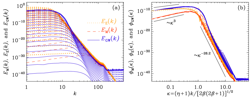
Figure 1: (a) $E_{\rm M}(k)$ (red lines), $E_{\rm E}(k)$ (orange lines), and $E_{\rm GW}(k)$ (blue lines) for Run A1. (b) $\phi_{\rm M}(\kappa)$ (red lines), $\phi_{\rm E}(\kappa)$ (orange lines), and $\phi_{\rm GW}(\kappa)$ (blue lines). The black straight lines denote the slopes $E_{\rm M}(k)\propto\kappa^{3}$ and $\propto\kappa^{1.7}$ for small $\kappa$.

In step II, for $\eta>1$, the conductivity $\sigma$ is finite and so the evolution of $\mathbf{E}$ can be omitted and the magnetic and GW fields are evolved by solving the MHD and GW equations, as described in previous papers (Roper Pol et al., 2020a, b), where the evolution equation for $\mathbf{A}$,

$$\frac{\partial\mathbf{A}}{\partial\eta}=\mathbf{u}\times\mathbf{B}+\sigma^{-1}\nabla^{2}\mathbf{A}$$ (10)

is solved in real space. This equation includes the induction effects from the velocity and the finite conductivity. It is solved together with (Brandenburg et al., 1996)

$$\frac{\partial\mathbf{u}}{\partial\eta}=-\mathbf{u}\cdot{\mathbf{\nabla}}\mathbf{u}-{1\over 4}{\mathbf{\nabla}}\ln\rho+{3\over 4\rho}\mathbf{J}\times\mathbf{B}+\mbox{\boldmath${\cal F}$}{}_{\nu}+\mbox{\boldmath${\cal F}$}{},$$ (11)

$$\frac{\partial\ln\rho}{\partial\eta}=-\frac{4}{3}\left({\mathbf{\nabla}}\cdot\mathbf{u}+\mathbf{u}\cdot{\mathbf{\nabla}}\ln\rho\right)+{\cal H},$$ (12)

where $\mbox{\boldmath${\cal F}$}{}=({\mathbf{\nabla}}\cdot\mathbf{u}+\mathbf{u}\cdot{\mathbf{\nabla}}\ln\rho)\mathbf{u}/3-[\mathbf{u}\cdot(\mathbf{J}\times\mathbf{B})+\mathbf{J}^{2}/\sigma]\mathbf{u}/\rho$, and ${\cal H}=[\mathbf{u}\cdot(\mathbf{J}\times\mathbf{B})+\mathbf{J}^{2}/\sigma]\rho$ are additional terms that are retained in the calculation, and $\mbox{\boldmath${\cal F}$}{}_{\nu}=2{\mathbf{\nabla}}\cdot(\rho\nu\mbox{\boldmath${\sf S}$}{})/\rho$ is the viscous force, where ${\sf S}_{ij}={\textstyle{1\over 2}}(u_{i,j}+u_{j,i})-{\textstyle{1\over 3}}\delta_{ij}{\mathbf{\nabla}}\cdot\mathbf{u}$ are the components of the rate-of-strain tensor with commas denoting partial derivatives, and $\nu$ is the kinematic viscosity. In all cases considered below, we assume a magnetic Prandtl number of unity, i.e., $\nu\sigma=1$. We recall that $a=\eta$ during the radiation-dominated phase, and therefore we have $a^{\prime\prime}/a=0$ in Equation (5).

In step II, the stress associated with the electric field is absent in the expression for ${\sf T}_{ij}$. Instead, the Reynolds stress $\gamma^{2}\rho u_{i}u_{j}$ now enters. Here, $\gamma$ is the Lorentz factor with $\gamma^{2}=1/(1-\mathbf{u}^{2})$.

For both steps I and II, we use the Pencil Code (Pencil Code Collaboration et al., 2021), which is primarily designed to solving large sets of partial differential equations on massively parallel computers using sixth-order finite differences and a third-order time stepping scheme. However, the code is versatile and allows the GW equations to be advanced analytically in Fourier space from one time step to the next; see the detailed description in Roper Pol et al. (2020a). In step I, we solve Equation (4) in a similar fashion as Equation (5), where the time advance from one time step to the next is done analytically; see Appendix C, where we describe the more general case with $\sigma\neq 0$. It should be emphasized that, although Equations (4) and (5) are linear for $\tilde{\mathbf{A}}$ and $\tilde{h}_{+/\times}$, respectively, the combined problem is not because $\tilde{T}_{+/\times}(\eta,\mathbf{k})$ depends quadratically on $\mathbf{E}$ and $\mathbf{B}$ through Equation (6).

In some of our simulations, the electromagnetic energy density exceeds 10% of the radiation energy density. This would be unrealistically large and those cases are only included for comparison with others of smaller electromagnetic energy density. Indeed, it would then no longer be obvious that the linearized GW equations are still applicable and that quadratic terms can be neglected. Although the fractional GW energy densities are always much below the fractional electromagnetic energy densities, it is conceivable that nonlinear effects could play a role in certain wavenumber ranges. The Pencil Code does allow for such nonlinear effects in the GW field to be incorporated. Preliminary studies suggest that nonlinear contributions to the stress begin to enhance the resulting GW energy spectra at large wavenumbers when the electromagnetic energy density reaches about 30% of the radiation energy density. However, such cases are not included in the present study and their details will be presented elsewhere.

3 Results

3.1 Evolution during step I

During reheating, the energies of various fields increase rapidly in power-law fashion, i.e., ${\cal E}_{i}(\eta)\propto(\eta+1)^{p_{i}}$ with $i={\rm M}$, ${\rm E}$, or ${\rm GW}$ for the magnetic, electric, and GW energies, respectively. Analytically, as shown in Appendix B, we expect $p_{\rm M}=p_{\rm E}=4\beta-2$, which is $27.2$, $25.2$, and $8.8$ for $\beta=7.3$, $6.8$, and $2.7$, respectively. The growth continues to occur at progressively smaller wavenumbers. The results are qualitatively similar for $\beta=2.7$, which is relevant to reheating at the QCD energy scale; see Appendix A. At all larger wavenumbers, the magnetic field oscillates in space and time, but does not increase on average. The GW field evolves in a similar fashion, but even more rapidly, and empirically with $p_{\rm GW}=2(p_{\rm M}-1)$.

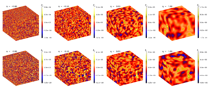
Figure 2: Visualizations of $B_{z}$ (top) and $h_{+}$ (bottom) on the periphery of the computational domain for Run A1 at $\eta=-0.8$, $-0.5$, $0$, and $1$ during step I. The color scale is symmetric about zero and adjusted with respect to the instantaneous extrema.

In Figure 1(a), we show for the case with $\beta=6.8$ magnetic, electric, and GW energy spectra in regular time intervals. The spectra collapse on top of each other when plotting them versus

$$\kappa(\eta)=(\eta+1)k/[2\beta(2\beta+1)]^{1/2}\equiv k/k_{\rm*}(\eta)$$ (13)

and multiplying by a compensating factor $(\eta+1)^{-(p_{i}+1)}$. Thus, we define (for $\eta\leq 1$)

$$\phi_{i}(\kappa)=(\eta+1)^{-(p_{i}+1)}E_{i}(k,\eta).$$ (14)

This implies ${\cal E}_{\rm M}(\eta)\equiv\int E_{M}(k,\eta)\,{\rm d}{}k\propto(\eta+1)^{p_{\rm M}}$ for the temporal growth of the ($k$-integrated) magnetic energy density for $\eta<1$. In Figure 2, we show visualizations of $B_{z}$ and $h_{+}$ on the periphery of the computational domain for Run A1. We see that the typical length scales of both fields increase with time. This is due to the fact that the destabilizing term $f^{\prime\prime}/f$ in Equation (4) decreases with time and remains important only on progressively larger length scales; see Equation (3).

We have also inspected visualizations of $\dot{h}_{+}$ and found that they looked virtually identical to those of $h_{+}$. Unlike step II, where this is not the case (discussed below), we have therefore not shown $\dot{h}_{+}$ here. However, we have looked at the local correlation between the two for each mesh point and found that $\dot{h}_{+}\approx sh_{+}$ with $s$ being compatible with $p_{\rm M}/(\eta+1)$. This suggests that the GW evolution is almost entirely dominated by the rapid algebraic increase at each point in space.

It also turned out that, as expected from the work of Sharma et al. (2017), the electric energy exceeds the magnetic energy by a certain factor. This factor depends on the value of $\beta$ and is about 8.6, 8.2, and 2.7 for $\beta=7.3$, 6.8, and 2.7, respectively.

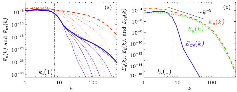
Figure 3: (a) Early times in the beginning of the radiation-dominated phase: $\eta=1$, $2$, $3$, $4$, $5$, and $20$ for Run A1. The last time at $\eta=20$ is shown as a thick red dashed line for $E_{\rm M}(k)$ and a thick blue solid line for $E_{\rm GW}(k)$. (b) Late times: $\eta=28$. The vertical file goes through $k_{*}$ defined in Equation (7).

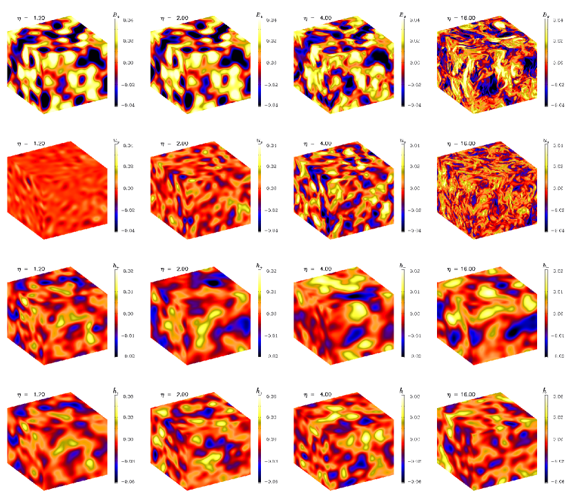
Figure 4: Visualizations of $B_{z}$, $u_{z}$, $h_{+}$, and $\dot{h}_{+}$ (from top to bottom) on the periphery of the computational domain for Run A1 at four times during step II. The color scale is different for each field, but the same at all times.

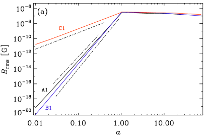
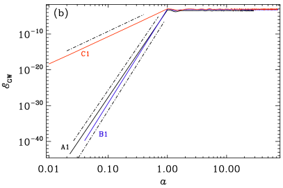
Figure 5: Comparison of Runs A1 (black line), B1 (blue line), and C1 (red line) showing the evolution (expressed in terms of $a$) of (a) $B_{\rm rms}$ (expressed in gauss), and (b) the ${\cal E}_{\rm GW}$. In (a), the dashed-dotted lines have slopes of 6.3, 6.8, and 2.2 for Runs A1, B1, and C1, respectively, and in (b) the slopes are 24.2, 26.2, and 7.8.

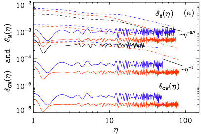
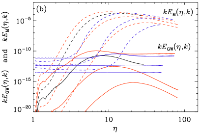
Figure 6: Evolution of (a) ${\cal E}_{\rm GW}$ and ${\cal E}_{\rm M}$ as solid and dashed lines, respectively, and (b) $kE_{\rm GW}(\eta,k)$ and $kE_{\rm M}(\eta,k)$, also as solid and dashed lines, respectively, with $k=40$ for Runs A1 (black line), B1–B3 (blue lines), and C1–C3 (red lines). In (a), the empirical decays $\propto\eta^{-0.7}$ and $\eta^{-1}$ are indicated.

Magnetic and electric fields still grow rapidly at the end of reheating, but only at large length scales. At $\eta=1$, we assume that the electric conductivity increases rapidly to sufficiently high values, so there will be no electric fields anymore, but there will be electric currents, $\mathbf{J}={\mathbf{\nabla}}\times\mathbf{B}$, and they will exert a Lorentz force, $\mathbf{J}\times\mathbf{B}$. We then switch to MHD and solve for the resulting velocity field, which facilitates a turbulent cascade toward smaller length scales. In Appendix D, we demonstrate quantitatively how a faster increase of conductivity reduces the magnetic energy loss during this transition into the high conductivity regime.

3.2 Evolution during step II

In all runs of step II, we have initially $\mathbf{u}=\ln\rho=0$. We chose $\nu=10^{-4}$, which was the smallest possible value that still allowed us to resolve the smallest length scales when $k^{-1}=1$ and $512^{3}$ mesh points were used. For two pairs of runs (Runs A1 and A2), we had to use $1024^{3}$ mesh points. Yet smaller values of $\nu$ and the magnetic diffusivity $\sigma^{-1}=\nu$ would be physically more realistic, but would require an even larger number of mesh points. As is commonly known in turbulence theory, this would only extend the turbulent cascade to smaller length scales, but would not strongly affect the rest of the turbulent inertial range.

The magnetic, kinetic, and GW spectra are shown in Figure 3. There is a gradual establishment of a turbulent cascade in magnetic and kinetic energy spectra approximately proportional to $k^{-2}$. However, during an intermediate stage of our investigations, we also have experimented with even larger values of the exponent $\beta$ and found that the turbulence in those cases is even more vigorous and can exhibit a $k^{-5/3}$ spectrum, suggestive of Kolmogorov-like turbulence; see Appendix E for an example.

The kinetic energy spectrum shows approximate equipartition at small length scales, i.e., $E_{\rm K}(k,\eta)\approx E_{\rm M}(k,\eta)$ for $k>k_{\rm*}(\eta)$. The GW energy spectrum shows a characteristic drop at the smallest unstable scale at the end of reheating, followed by an approximate power-law spectrum at higher wavenumbers. Such a drop was found particularly clearly in recent GW simulations driven by an underlying magnetic field that was forced at very large length scales (Brandenburg et al., 2021a). More generally, such a drop is seen to various extents in all GW simulations sourced by monochromatically driven vortical turbulence; see, for example, Figure 6 of Roper Pol et al. (2020a). By comparing with their Figure 4, one sees that this drop is not seen when a turbulence spectrum is initialized through an initial condition rather than through gradual driving. This implies a sudden jump in time, even at small length scales, which is unrealistic. Our simulations predict for the first time a natural time scale of the temporal increase of the stress, especially at high wavenumbers. The relatively low amplitude of GWs at these high wavenumbers suggests that GW generation is predominantly a large-scale phenomenon and therefore also not strongly dependent on the exact details at small length scales. Another reason for this sharp drop at higher $k$ is that the turbulent stress develops only later, when the $1/a$ factor on the right-hand side of Equation (5) has diminished its effect.

We find the ratio between magnetic and kinetic energies to be only about 1.3 and not as large as in some earlier simulations of turbulence driven by an initial magnetic field with a spectrum peaked at intermediate wavenumbers, where $E_{\rm M}\propto k^{-2}$ was found. In the present case, the spectrum is peaked at large length scales, so there is no possibility for the magnetic field to display marked inverse transfer to larger length scales, as was the case in simulations of Brandenburg et al. (2015), who found inverse transfer even without magnetic helicity; see also Zrake (2014) for relativistic turbulence simulations.

Earlier work on inflationary magnetogenesis presumed the appearance of a scale-invariant spectrum proportional to $k^{-1}$; see, e.g., Kahniashvili et al. (2012, 2017). In the present case, the magnetic field along with velocity fluctuations are being driven by a turbulent cascade and fed by the large-scale magnetic field. As already noted by Sharma et al. (2017, 2018), the magnetic field has a blue $k^{3}$ spectrum at small wavenumbers, $k<k_{*}(1)$. During the early part of the radiation-dominated phase, we see that the peak gradually shifts to smaller wavenumbers, so the initial $k^{3}$ spectrum can hardly be recognized within the limited wavenumber range accessible to our simulations; see Figure 3(b).

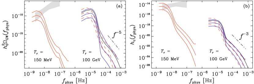
Figure 7: (a) $h_{0}^{2}\Omega_{\rm GW}(f_{\rm phys})$ and (b) $h_{c}(f_{\rm phys})$ for Runs A1 (black lines) and B1–B3 (blue lines) for $T_{\rm r}=100\,{\rm GeV}$ and Runs C1–C3 (red lines) for $T_{\rm r}=150\,{\rm MeV}$. To compare the two energy scales, we show Runs C1–C3 also for $T_{\rm r}=100\,{\rm GeV}$ (red dashed lines). The gray region marks the $2\sigma$ confidence contour for the 30 frequency power law of the NANOGrav 12.5-year data set.

In Figure 4, we show visualizations of $B_{z}$, $u_{z}$, $h_{+}$, and $\dot{h}_{+}$ on the periphery of the computational domain for Run A1 during step II at $\eta=1.2$, 2, 4, and 16. We see that for $\eta\leq 2$, the magnetic field has almost not changed at all. The velocity is still small, but begins to become important for $\eta>2$. Fully developed turbulence is seen at $\eta=16$. However, the strain field and its time derivative are not visibly affected by the fully developed turbulence.

3.3 Time series for different values of $\beta$

In Figure 5, we show the evolution of $B_{\rm rms}$ and ${\cal E}_{\rm GW}$ both for steps I and II as a double-logarithmic plot. Since $\eta$ can be negative, we express time in terms of $a=(\eta+1)^{2}/4$ for $\eta<1$ (and $a=\eta$ otherwise). Owing to the quadratic scaling in time and the additional quadratic scaling of magnetic energy with $B_{\rm rms}$ in step I, the slopes of $6.8$, $6.3$, and $2.2$ for Runs A1–C1 correspond to the exponents of $p_{\rm M}=27.2$, $25.2$, and $8.8$, respectively. In step II, we see that $B_{\rm rms}$ displays a comparatively slow decay relative to the rapid increase for $\eta<1$. The decay for $\eta\gg 1$ follows a power law $\propto\eta^{-1}$ for $\beta=7.3$, and $\propto\eta^{-0.7}$ for $\beta=2.3$; see Figure 6(a). This panel also shows that the GW energy fluctuates in time, but is otherwise statistically stationary. There is, however, a systematic wiggle in all curves of ${\cal E}_{\rm GW}$ at around $\eta=1.05$. This is caused by the discontinuity in $a^{\prime\prime}/a$ and $f^{\prime\prime}/f$ at $a=1$. In Appendix F, we examine the effects of removing the discontinuity on the occurrence of oscillations and we also study the effects on the GW energy spectrum between the end of step I and the beginning of step II.

A decay of ${\cal E}_{\rm M}$ proportional to $\eta$ is also what has been obtained in earlier simulations of magnetically dominated decaying turbulence (Brandenburg & Kahniashvili, 2017), but the slower decay proportional to $\eta^{-0.7}$ has only been seen in the presence of magnetic helicity. Here, however, the magnetic helicity is zero. The reason for this slower decay is probably connected with the absence of an extended subinertial range in our simulations, where $k_{\rm*}(1)$ is too close to the minimal wavenumber $k_{1}$. If we allowed for more mesh points and larger domains, the expected $\eta^{-1}$ decay should be recovered.

Our simulations yield a temporal increase of the GW energy at length scales smaller than $k_{*}^{-1}(\eta)$ for $\eta>1$. In the absence of turbulence, GWs would only have existed on large length scales. To see the development at intermediate length scales more clearly, we compare in Figure 6 the temporal evolution of the GW and magnetic energy densities in panel (a), and in panel (b) the GW and magnetic energies at the wavenumber $k=40$. We see that magnetic and GW energies increase with time. The larger the magnetic energy at $\eta=1$, the more rapidly ${\cal E}_{\rm GW}(\eta)$ increases and the larger is their final GW energy. There is considerable spread in the final values of the scale-dependent GW energy densities, while the spread in the scale-dependent magnetic energy densities is much less. Unlike the total, wavenumber-integrated GW energy, which is nearly perfectly statistically stationary already after a short time, the scale-dependent values are in some cases not yet steady and are still decreasing after having reached a certain maximum value.

Table 1: $C_{1}$, $C_{2}$, and $C_{*}$ for two values of $T_{\rm r}$.

$T_{\rm r}$	$H_{*}/H_{0}=C_{1}$	$a_{*}/a_{0}=C_{2}$	$C_{*}=C_{1}^{2}C_{2}^{4}$
$100\,{\rm GeV}$	$6.4\times 10^{27}$	$8.0\times 10^{-16}$	$1.6\times 10^{-5}$
$150\,{\rm MeV}$	$5.6\times 10^{21}$	$1.0\times 10^{-12}$	$3.1\times 10^{-5}$

Table 2: Summary of simulation parameters and properties.

					radiation dominated		$B_{\rm rms}$	$T_{\rm r}$	scaled to the present time
Run	$B_{0}$	$\beta$	${\cal E}_{\rm EM}$	${\cal E}_{\rm E}/{\cal E}_{\rm M}$	${\cal E}_{\rm GW}$	$h_{\rm rms}$	[$\mu$G]	[GeV]	${\Omega}_{\rm GW}$	$h_{\rm c}$
A1	$1\times 10^{-17}$	$6.8$	$0.12$	$32.7$	$3.3\times 10^{-4}$	$1.7\times 10^{-2}$	$0.24$	$100$	$5.4\times 10^{-9}$	$1.4\times 10^{-17}$
A2	$1\times 10^{-17}$	$6.8$	$0.12$	$32.7$	$3.2\times 10^{-4}$	$1.7\times 10^{-2}$	$0.24$	$100$	$5.3\times 10^{-9}$	$1.4\times 10^{-17}$
A3	$1\times 10^{-17}$	$6.8$	$0.12$	$32.7$	$5.9\times 10^{-5}$	$8.5\times 10^{-3}$	$0.24$	$100$	$9.7\times 10^{-10}$	$6.8\times 10^{-18}$
B1	$1\times 10^{-18}$	$7.3$	$0.18$	$34.4$	$6.3\times 10^{-4}$	$2.3\times 10^{-2}$	$0.28$	$100$	$1.0\times 10^{-8}$	$1.9\times 10^{-17}$
B2	$5\times 10^{-19}$	$7.3$	$0.05$	$34.4$	$3.9\times 10^{-5}$	$5.8\times 10^{-3}$	$0.14$	$100$	$6.3\times 10^{-10}$	$4.6\times 10^{-18}$
B3	$2\times 10^{-19}$	$7.3$	$0.01$	$34.4$	$2.4\times 10^{-6}$	$1.4\times 10^{-3}$	$0.07$	$100$	$3.9\times 10^{-11}$	$1.1\times 10^{-18}$
C1	$5\times 10^{-7}$	$2.7$	$0.07$	$10.8$	$8.6\times 10^{-4}$	$3.7\times 10^{-2}$	$0.31$	$0.15$	$2.7\times 10^{-8}$	$3.7\times 10^{-14}$
C2	$2\times 10^{-7}$	$2.7$	$0.017$	$10.8$	$5.3\times 10^{-5}$	$9.1\times 10^{-3}$	$0.15$	$0.15$	$1.6\times 10^{-9}$	$9.1\times 10^{-15}$
C3	$1\times 10^{-7}$	$2.7$	$0.004$	$10.8$	$3.3\times 10^{-6}$	$2.3\times 10^{-3}$	$0.08$	$0.15$	$1.0\times 10^{-10}$	$2.3\times 10^{-15}$

3.4 Present-day frequency spectra

To compute the strain at the present time, we have to multiply our values of $h_{\rm rms}$ by the ratio $C_{1}=a_{*}/a_{0}$, where $a_{*}$ and $a_{0}$ are the scale factors at reheating and the present time, respectively. To obtain the GW energy at the present time, we also have to take the Hubble factor $C_{2}=H_{*}/H_{0}$ into account, where $H_{*}$ and $H_{0}$ are the Hubble parameters at reheating and the present time, respectively. Thus, we have to multiply our value of ${\cal E}_{\rm GW}$ by the dilution factor, $C_{*}\equiv(a_{*}/a_{0})^{4}(H_{*}/H_{0})^{2}\equiv C_{1}^{4}C_{2}^{2}$; see Roper Pol et al. (2020b). The values of $C_{1}$, $C_{2}$, and $C_{*}$ are given in Table LABEL:Tconversion, and are also consistent with those used earlier (Brandenburg et al., 2021a; He et al., 2021).

The resulting GW energy and strain spectra, scaled to the present time, are shown in Figure 7, where we show the frequency spectra

$$h_{0}^{2}\Omega_{\rm GW}(f_{\rm phys})=C_{*}kE_{\rm GW}(k);\;h_{c}(f_{\rm phys})=C_{2}h_{\rm rms}(k)$$ (15)

with $f_{\rm phys}(k)=H_{*}k/2\pi a_{0}$ being the physical frequency for Runs A1–C3; see also Table LABEL:Tsummary for the parameters. In Run A3, the GW field has been reset to zero at $\eta=1$ (see Section 3.5), but in all other cases, $\tilde{h}_{+/\times}$ and $\tilde{h}^{\prime}_{+/\times}$ have been inherited from step I. In Figure 7, we have also indicated the $2\sigma$ confidence contour for the 30 frequency power law of the NANOGrav 12.5-year data set (Arzoumanian et al., 2020); see Brandenburg et al. (2021a) for the details of the determination of the present contours.

Runs B1–B3 have the same value of $\beta$, but different initial magnetic field strengths, resulting also in different values of the maxima of ${\cal E}_{\rm E}$ and ${\cal E}_{\rm M}$. We recall that these values are automatically the fractional magnetic energy density relative to the radiative energy density, which is also equal to the critical energy density for a spatially flat Universe. Our choice of $\beta=7.3$ applies specifically to the case with ${\cal E}_{\rm EM}\equiv{\cal E}_{\rm E}+{\cal E}_{\rm M}=0.01$, which corresponds to the case of Run B3. For Run B1, on the other hand, where ${\cal E}_{\rm EM}$ is larger, the value $\beta=6.8$ should have been more appropriate. Such a case is presented in Table LABEL:Tsummary as Run A1. However, we see that the differences between Runs A1 and B1 are minor. We can therefore conclude that the precise choice of $\beta$ is not critical for the final outcome of our models.

Figure 7 shows that, even well beyond the drop in $h_{0}^{2}\Omega_{\rm GW}(f_{\rm phys})$, there continues to be a fairly steep fall-off proportional to $f^{-5}$. Such a strong decline was also seen in the earlier work of Roper Pol et al. (2020b); see their Figure 6. This is much steeper than the $f^{-8/3}$ law obtained for the GW spectrum when a turbulent source with a Kolmogorov-type spectrum is switched on as the initial condition. In Appendix E, we demonstrate that such a shallow fall-off can be reproduced by assuming an artificially strong source where the magnetic energy exceeds 10% of the radiation energy density and therefore the electric field energy density just prior to the commencement of MHD would have been as large as the radiation energy density of the universe.

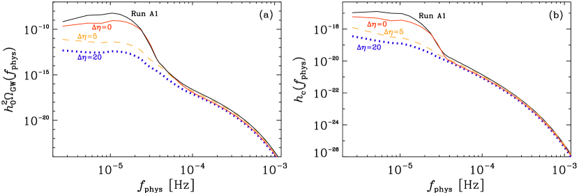
Figure 8: (a) $h_{0}^{2}\Omega_{\rm GW}(f_{\rm phys})$ and (b) $h_{c}(f_{\rm phys})$ for Run A1 compared with runs where the GW field from step I has been ignored, so $\tilde{h}_{+/\times}=\tilde{h}^{\prime}_{+/\times}=0$ has been set and the hydromagnetic stress was applied instantaneously (Run A3, $\Delta\eta=0$, red solid line), or gradually over a time span $\Delta\eta=5$ (orange dashed line) or $\Delta\eta=20$ (blue dotted line).

Earlier work by Roper Pol et al. (2020b) did already demonstrate that the Reynolds stress in ${\sf T}_{ij}$ contributes only about 10% to the resulting GW energy. In Table LABEL:Tsummary, we have listed Run A2, where the Reynolds stress is omitted in ${\sf T}_{ij}$. It turns out that the GW energy is indeed reduced, but only by a few percent, so the Reynolds stress is here completely unimportant. This is partially explained by the fact that the resulting turbulence develops almost entirely on small scales (see Figure 4), where the effect on GWs is small.

We see that most of the power occurs at frequencies of about $20\,\mu{\rm Hz}$ ($10\,{\rm nHz}$) for $T_{\rm r}=100\,{\rm GeV}$ ($150\,{\rm MeV}$), followed by a drop of GW energy and strain by four and two orders of magnitude, respectively. This may suggest that the turbulent production of GWs is only moderately effective in converting the turbulent energy from the forward cascade to GW energy. In the following, we shall look at this more quantitatively.

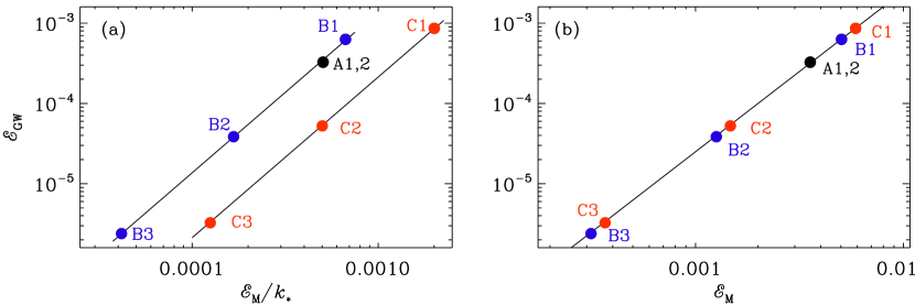
Figure 9: (a) Dependence of ${\cal E}_{\rm GW}$ on ${\cal E}_{\rm M}/k_{*}$ for Runs A1 and A2 (black), B1–B3 (blue), and C1–C3 (red). The solid line is a quadratic fit through the black and blue symbols, ${\cal E}_{\rm GW}=(q{\cal E}_{\rm M}/k_{*})^{2}$, with $q=37$ and through the red symbols with $q=14.6$. (b) Similar to panel (a), but plotted versus ${\cal E}_{\rm M}$. Here, the solid line corresponds to the fit given by Equation (17).

3.5 Significance of using the GW field from step I

Except for the recent simulations of Brandenburg et al. (2021c), previous work on numerical investigations of GW generation from hydrodynamic or MHD turbulence assumed that turbulence was either switched on instantaneously or it was gradually being produced; see Roper Pol et al. (2020b) for comparisons of such models. In either case, the GW field was always initially zero, i.e., $\tilde{h}_{+/\times}=\tilde{h}^{\prime}_{+/\times}=0$. Here, by contrast, both $\tilde{h}_{+/\times}$ and $\tilde{h}^{\prime}_{+/\times}$ are finite at $\eta=1$. As suggested in the introduction, this can make a difference and could underestimate the resulting GW energy. To study this in more detail, we now perform an additional simulation (Run A3 in Table LABEL:Tsummary) with $\tilde{h}_{+/\times}=\tilde{h}^{\prime}_{+/\times}=0$ at $\eta=1$, using just the magnetic field from step I. We see that the GW energy is now about 10 times weaker than otherwise (Run A1).

The resulting spectra are shown in Figure 8, where we plot the GW energy and strain for a series of models where we turned on the stress either instantaneously (as in Run A3) or gradually using a linearly varying profile function that multiplies the stress by a factor that linearly grows to unity within a time to span $\Delta\eta$. Thus, we replace

$$\tilde{T}_{+/\times}\to\frac{\eta-1}{\Delta\eta}\tilde{T}_{+/\times}\quad\mbox{for $1<\eta<1+\Delta\eta$}.$$ (16)

The case of instantaneously switching on the stress corresponds then to $\Delta\eta\to 0$. The original Run A1 is shown for comparison.

We see that an instantaneously switched on stress produces a GW spectrum that agrees with the original one at high wavenumbers, and only at low wavenumbers is there a small deficiency in GW energy and strain. This shows that the inheritance of the GW field from step I is of relatively minor importance. The agreement at high wavenumbers is no surprise because at those high $k$ values, the GW field was absent at $\eta=1$. The speed of regeneration of the GW field at low $k$ is more surprising, but the qualitative agreement with Run A1 is probably related to the fact that the generation in step I is so rapid that only the last moment has a decisive effect on the GW field. This then also demonstrates that the reason for the rapid drop in spectral GW energy and strain past the peak wavenumber is, at least in part, a consequence of the existence of magnetic fields only for $k<k_{\rm*}(1)$ at $\eta=1$.

To examine this further, we now describe two models where $\Delta\eta=5$ and $20$. We see that the dominance of the GW energy and strain at small $k$ diminishes and that also the sharp drop in spectral GW energy and strain becomes smaller. Whether the remaining lack of continuity of the GW spectrum at $k\approx k_{\rm*}(1)$ is caused by the limited vigor of turbulence is unclear. Nevertheless, the existence of the sharp drop in spectral GW energy and strain seems to be a physical effect that was not previously anticipated in relic GW modeling.

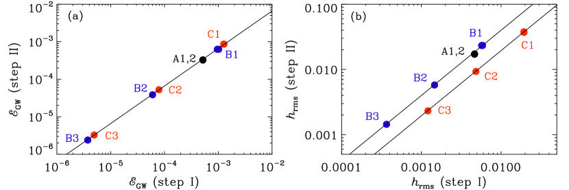
Figure 10: Dependence of the final values in step II of (a) ${\cal E}_{\rm GW}$ and (b) $h_{\rm rms}$ on those at the end of step I. In (a) the solid line denotes ${\cal E}_{\rm GW}(\mbox{step~{}II})=0.66\,{\cal E}_{\rm GW}(\mbox{step~{}I})$, while in (b) the upper solid line denotes $h_{\rm rms}(\mbox{step II})=4.0\,h_{\rm rms}(\mbox{step I})$ for $\beta=7.3$ and the lower solid line denotes $h_{\rm rms}(\mbox{step~{}II})=1.9\,h_{\rm rms}(\mbox{step~{}I})$ for $\beta=2.7$.

3.6 GW efficiency and scaling with ${\cal E}_{\rm M}$

The GW energy of our runs scales approximately quadratically with magnetic energy. Following earlier work (Roper Pol et al., 2020b; Brandenburg et al., 2021b), we confirm a relation of the form ${\cal E}_{\rm GW}=(q{\cal E}_{\rm M}/k_{\rm c})^{2}$, where $q$ is the efficiency and $k_{\rm c}$ is the characteristic wavenumber, for which the value $k_{\rm c}=k_{\rm*}(1)$ has been used. The values of ${\cal E}_{\rm M}$ range between 0.03% and 0.5% of the radiation energy density.

With that, we find for Runs B1–B3 an efficiency parameter of $q=37$, and smaller values of $14.6$ for Runs C1–C3, where $\beta=2.7$; see Figure 9(a). The obtained efficiency $q$ is smaller for smaller values of $\beta$, suggesting a dependence between $q$ and $\beta$. In particular, using $q=5\beta$ appears to be a good empirical description of our data. However, since $k_{\rm*}$ also depends on $\beta$, and the ratio $\beta/k_{\rm*}(1)$ is about unity, a good fit to the data is then given by

$${\cal E}_{\rm GW}\approx\,(5\,{\cal E}_{\rm M})^{2}.$$ (17)

We thus see that the previously obtained $k_{\rm c}$ dependence of ${\cal E}_{\rm GW}$ (Roper Pol et al., 2020b; Brandenburg et al., 2021a, b) can just be subsumed into the dependence on ${\cal E}_{\rm M}$, at least in the present case.

3.7 Change of GW amplitude between steps I and II

It turns out that the final values of ${\cal E}_{\rm GW}$ and $h_{\rm rms}$ are not the same as those at the end of step I. However, they are proportional to each other in such a way that the final ${\cal E}_{\rm GW}$ in step II is about 0.66 times the value at the end of step I, and the final $h_{\rm rms}$ in step II is about four times the value at the end of step I for $\beta=7.3$ and about twice the value at the end of step I for $\beta=2.7$; see Figure 10.

4 Conclusions

We have presented three-dimensional direct numerical simulations of inflationary magnetogenesis and relic GW production during the end of a matter-dominated reheating era, and the subsequent evolution in the beginning of the radiation-dominated era. As expected based on earlier analytic work, electromagnetic fields grow in power-law fashion, with the electric field exceeding the magnetic one. GWs are driven by the electromagnetic stress and also grow in power-law fashion. The growth terminates with the beginning of the radiation-dominated era, when high electric conductivity leads to a turbulent MHD cascade. Vigorous motions produce small-scale hydromagnetic stresses, but they are too weak to have a significant effect on the GW spectrum, which therefore remains being dominated by large-scale features. This is seen as a marked drop in the GW energy at present-day frequencies of around $20\,\mu{\rm Hz}$ ($3\,{\rm nHz}$) for a reheating temperature of $100\,{\rm GeV}$ ($150\,{\rm MeV}$).

In comparison with earlier analytical work estimating the efficiency of GW production from inflationary magnetogenesis by Sharma et al. (2020), our present work has highlighted some important aspects and discrepancies with numerical modeling. There is, most importantly, the spectral drop in the GW spectra above the peak wavenumber $k_{\rm*}(1)$, which remained almost unchanged after $\eta=1$. The drop is clearly seen both in wavenumber spectra (Figure 3) and in the diagnostic frequency spectra (Figure 7). Here, the frequency spectra have been obtained from the wavenumber spectra, but let us emphasize in this connection that the numerical equivalence between the two was recently confirmed and that even a spectral drop similar to that seen here is faithful reproduced from the temporal Fourier transform of the time series (He et al., 2021). Discrepancies between temporal and spatial spectra can occur, however, when the dispersion relation of GWs is no longer linear (for example for finite graviton mass), or when there is a long-term effect from the stress associated with the slowly decaying turbulence (He et al., 2021). This effect only plays a very small role because most of the GW energies are dominated by contributions from small wavenumbers. Nevertheless, it could explain small discrepancies between strain spectra and the anticipated GW energy spectra at frequencies above the spectral drop of the GW energy. This drop can then reveal subtle features associated with the turbulent inertial range, but the aforementioned differences should disappear at very late times, well beyond what has been simulated so far, and would not be observationally significant.

The spectral drop in GW energy is not a particular feature associated with inflationary magnetogenesis, but it appears to be a feature associated with turbulence driven at scales comparable to the horizon scale with $k\approx 1$. It should be emphasized that, at the level of the present model, there is no immediate association between the value of the reheating temperature and the physics of phase transitions. In particular, there is no obvious feature in the resulting GW spectra from magnetogenesis during reheating and any other hypothetical source of turbulence. This can be seen by comparing the present GW spectra with those of Brandenburg et al. (2021a), where turbulence was driven by an assumed low wavenumber forcing function. A possible difference may lie in the dependence of ${\cal E}_{\rm GW}$ on ${\cal E}_{\rm M}$, which does not involve an independent scaling with the inverse of the characteristic wavenumber $k_{\rm c}$. This finding came as somewhat of a surprise, but it may just mean that, in the present model, the efficiency parameter does indeed scale with $\beta$. Preliminary experiments with helical magnetogenesis (Brandenburg et al., 2021d) suggest that the $1/k_{\rm c}$ scaling remains in general justified.

A particular problem in previous numerical modeling of GW production by magnetic stresses laid in the fact that most of the GW energy resides at small wavenumbers or large length scales. This was particularly evident in some of the simulations describing the chiral magnetic effect; see Run B1 of Brandenburg et al. (2021c) for such an example. This meant that such results remained sensitive to the value of $k_{1}$ and thus the choice of the size of the computational domain. In the present work, we have alleviated this problem by extending our domain to larger length scales, so that the spectral peak was still well within the domain of the model. The strength of the underlying magnetic field was then only limited by the condition that the electromagnetic energy should not exceed about 10% of the radiation energy density at the end of reheating. Owing to the subsequent emergence of a turbulent cascade, the magnetic energy is then being fed into smaller length scales. This leads to a temporal growth of both magnetic and GW energies at subhorizon length scales. However, the strength of GWs at small length scales remained weak compared with that at larger length scales. We have not yet seen a strong dependence on the numerical resolution. In fact, while both velocity and magnetic fields showed a well-resolved fine structure, the strain field and also its time derivative remained dominated by large-scale features. It is conceivable that even higher numerical resolution would be needed to produce sufficiently rapid variations at small length scales to enhance it GW production at those small scales, but at the moment there is no evidence for this.

An important extension of the present work is to consider helical magnetogenesis (Turner & Widrow, 1988; Garretson et al., 1992; Field & Carroll, 2000; Anber & Sorbo, 2006; Campanelli, 2009; Caprini & Sorbo, 2014; Adshead et al., 2016; Sobol et al., 2019; Adshead et al., 2020a, b). These authors considered an additional chiral symmetry breaking term involving the dual Faraday tensor in the Lagrangian; see also the papers by Sharma et al. (2018) and Okano & Fujita (2021). Helical magnetic fields decay more slowly than nonhelical ones and are therefore more likely to survive until the present time; see Figure 11 of Brandenburg et al. (2017). It would then also be interesting to see whether there are any other similarities with magnetogenesis from the chiral magnetic effect (Brandenburg et al., 2021c), in addition to the relation between the GW efficiency and the exponent $\beta$ identified in the present work.

Appendix A Relation between $\beta$ and the reheating temperature

At the end of the introduction, we stated that the values of $\beta=7.3$ and $2.7$ are appropriate for a reheating temperatures of $100\,{\rm GeV}$ and $150\,{\rm MeV}$. Here, we provide the details of this calculation.

To compute $\beta$ for a given reheating energy scale, $T_{\rm r}$, we follow the formalism of Sharma et al. (2017). The first step is to calculate the Hubble parameter during inflation, $H_{\rm f}$. It is related to $T_{\rm r}$ through their Equation (51), which we state here in corrected form as

$$\ln\left[\displaystyle{\frac{C+D}{{\cal E}_{\rm EM}}\left(\frac{g_{0}}{g_{r}}\right)^{\!\frac{2\alpha}{3}}\!\!\left(\frac{g_{r}\pi^{2}}{30}\right)^{\frac{\!\!4+\alpha}{3}}}\right]\!+134\alpha\!+(2\alpha+4)\ln\displaystyle{\frac{H_{f}}{T_{r}}}$$

$$-\displaystyle{\frac{7+\alpha}{3}\ln\left(\frac{3H_{f}^{2}}{8\pi G}\frac{1}{T_{r}^{4}}\right)}=0,$$ (A1)

where $C$ and $D$ are functions of $\alpha$ and $\beta$, whose values are amended by additional $\beta$-dependent factors that take into account that the spectrum peaks not at the Hubble wavenumber, as assumed in Sharma et al. (2017), but at $k=k_{\rm*}$. For $\alpha=2$, the numerical values are $C=0.01266\,\beta(\beta+1/2)$ and $D=0.0063\,[\beta(\beta+1/2)/(2\beta+1/2)]^{2}$. In Equation (A), we have corrected the following typo relative to the expression given by Sharma et al. (2017): the $(C+D)/g_{r}$ factor in their Equation (51) is replaced by $(C+D)/(g_{r}\pi^{2}/30)$. By incorporating this correction and combining it with $(g_{r}\pi^{2}/30)^{(7+\alpha)/3}$, their exponent $(7+\alpha)/3$ becomes $(4+\alpha)/3$ instead; see Equation (A). We have also incorporated the parameter ${\cal E}_{\rm EM}$, which represents the ratio of the electromagnetic energy density to the background. This value was taken to be unity in Equation (51) of Sharma et al. (2017).

Given an estimate for $H_{f}$, the values of $N_{r}$ and $N$ are obtained from the expressions

$$N_{r}=\frac{1}{3}\ln\left[\frac{90\,H^{2}_{f}}{8\pi G\pi^{2}g_{r}T_{r}^{4}}\right],$$ (A2)

and

$$N+N_{r}=66.9-\ln\left(\frac{T_{r}}{H_{f}}\right)-\frac{1}{3}\ln\frac{g_{r}}{g_{0}}.$$ (A3)

which then yields $\beta=\alpha N/N_{\rm r}$; see Table LABEL:Tbeta2 for examples considered in this paper.

Table 3: $\beta$ for different values of $T_{r}$.

$T_{r}$	${\cal E}_{\rm EM}$	$H_{\rm f}$ [GeV]	$N_{r}$	$N$	$\beta$
100 GeV	0.01	$1.56\times 10^{-8}$	9.3	33.9	7.3
100 GeV	0.1	$5.00\times 10^{-8}$	10.1	34.4	6.8
150 MeV	0.01	$1.70\times 10^{-2}$	27.2	36.5	2.7

Appendix B Initial condition for magnetic and electric energy spectrum during matter-dominated era

In Section 2, we stated that the initial magnetic energy spectrum for $k<k_{\rm*}(\eta)$ is proportional to $k^{3}$. Here, we provide the details and discuss the $\beta$ dependence of the steep slope for $k>k_{\rm*}(\eta)$.

We discuss here the initial condition for the numerical simulations in the post-inflation matter-dominated era. The initial magnetic and electric field spectra can be understood by the following argument. For $\alpha=2$, the magnetic field spectrum is scale-invariant during inflation. However, the scale-invariant part does not contribute to the growing solution in the post-inflation matter-dominated era. Only to the next order, there is a contribution proportional to $k^{3}$. Therefore, for the scales of interest, there is only the $k^{3}$ spectrum at super-Hubble scales. Using Equation (9) and (31) in (Sharma et al., 2017), it is concluded that the magnetic energy spectrum for a particular mode $k$ grows with time as $\propto(\eta+1)^{4\beta+2}$ until the mode satisfies the condition $k(\eta+1)\leq\sqrt{2\beta(2\beta+1)}$. Defining $\eta_{k}$ as the time for which the mode $k$ obeys $k(\eta+1)=\sqrt{2\beta(2\beta+1)}$, the initial condition for the magnetic energy spectrum is then given by

$$E_{\rm M}\propto\left\{\begin{array}[]{lr}k^{3}(\eta+1)^{(4\beta+2)},&k\leq k_{*}(\eta),\\ k^{3}(\eta_{k}+1)^{(4\beta+2)}\propto k^{1-4\beta},&k\geq k_{*}(\eta).\end{array}\right.$$ (B1)

In the above expression, $\eta_{k}$ represents the time for the mode $k$ when $k(\eta+1)=1$. Similarly, the initial condition for the electric energy spectrum is given by

$$E_{\rm E}\propto\left\{\begin{array}[]{lr}k(\eta+1)^{4\beta},&k\leq k_{*}(\eta),\\ k(\eta_{k}+1)^{4\beta}\propto k^{1-4\beta},&k\geq k_{*}(\eta).\end{array}\right.$$ (B2)

To get the total magnetic energy density, we can integrate Equation (B1) over $k$. Since the magnetic energy spectrum falls very steeply for $k>k_{\rm*}(\eta)$, taking $k_{\rm*}$ as the upper limit of the integration is a good approximation. Thus, we have

$$\int_{0}^{k_{\rm*}(\eta)}E_{\rm M}(k)\,{\rm d}{}k\propto k_{\rm*}(\eta)^{4}(\eta+1)^{4\beta+2}\propto(\eta+1)^{4\beta-2},$$ (B3)

which is well obeyed by the numerical results.

Appendix C Solving the Maxwell equation

At the end of Section 2, we described the numerical approach to solving Equation (4) and highlighted the analogy to solving Equation (5). Here, we give the details.

In the initial stage of this project, we solved the wave equation for $\mathbf{A}$ with $\sigma=0$ using the default sixth-order finite differences of the Pencil Code using the module special/disp_current. However, we noticed artificial degrading of the solution at small length scales—similarly to what was experienced when solving the GW equation in real space; see Roper Pol et al. (2020a) for details. Therefore, we decided to solve the Maxwell equation in Fourier space. Assuming ${\rm i}\mathbf{k}\cdot\tilde{\mathbf{A}}={\rm i}\mathbf{k}\cdot\tilde{\mathbf{E}}=0$, we have $\tilde{\mathbf{A}}^{\prime\prime}+\sigma\tilde{\mathbf{A}}^{\prime}+k^{2}\tilde{\mathbf{A}}=0$ with the characteristic equation $\lambda^{2}+\lambda\sigma+k^{2}=0$ and eigenvalues $\lambda_{\pm}=(-\sigma\pm D)/2$, where $D=\sqrt{\sigma^{2}-4k^{2}}$. If $\sigma=0$, then $D=2{\rm i}k$ and $\lambda_{\pm}=\pm{\rm i}k$.

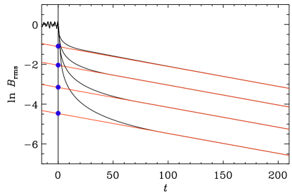
Figure 11: Decay of $\ln B_{\rm rms}$ for a linearly increasing conductivity.

Figure 12: Decay of $l=\ln B_{\rm rms}$ on the slope $s$ for a linearly increasing conductivity.

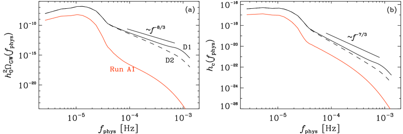
Figure 13: (a) $h_{0}^{2}\Omega_{\rm GW}(f_{\rm phys})$ and (b) $h_{c}(f_{\rm phys})$ for Runs A1 (red lines) and D1 and D2 (blue lines) for $T_{\rm r}=100\,{\rm GeV}$. The theoretically anticipated slopes for Kolmogorov-type turbulence are indicated as well.

Table 4: Comparison between Runs D1 and D2 with Run A1.

					radiation dominated		$B_{\rm rms}$	$T_{\rm r}$	scaled to the present time
Run	$\nu$	$\beta$	${\cal E}_{\rm EM}$	${\cal E}_{\rm E}/{\cal E}_{\rm M}$	${\cal E}_{\rm GW}$	$h_{\rm rms}$	[$\mu$G]	[GeV]	${\Omega}_{\rm GW}$	$h_{\rm c}$
A1	$1\times 10^{-17}$	$6.8$	$0.131$	$8.2$	$4.04\times 10^{-4}$	$2.03\times 10^{-2}$	$0.48$	$100$	$6.64\times 10^{-9}$	$1.62\times 10^{-17}$
D1	$2\times 10^{-21}$	$10$	$1.4$	$12$	$9.91\times 10^{-3}$	$8.25\times 10^{-2}$	$1.3$	100	$1.63\times 10^{-7}$	$6.58\times 10^{-17}$
D2	$5\times 10^{-21}$	$10$	$1.4$	$12$	$9.86\times 10^{-3}$	$8.27\times 10^{-2}$	$1.3$	100	$1.62\times 10^{-7}$	$6.60\times 10^{-17}$

Analogously to our solution of the GW equation (Roper Pol et al., 2020a) we solve the equation for $\tilde{\mathbf{A}}$ from one time $t$ to the next $t+\delta t$. We then make the following ansatz

$$\tilde{\mathbf{A}} = \tilde{\mathbf{A}}_{+}e^{\lambda_{+}\delta\eta}+\tilde{\mathbf{A}}_{-}e^{\lambda_{-}\delta\eta},$$ (C1)

$$\tilde{\mathbf{E}} = -\tilde{\mathbf{A}}_{+}\lambda_{+}e^{\lambda_{+}\delta\eta}-\tilde{\mathbf{A}}_{-}\lambda_{-}e^{\lambda_{-}\delta\eta},$$ (C2)

where the coefficients $\tilde{\mathbf{A}}_{+}$ and $\tilde{\mathbf{A}}_{-}$ are determined from $\tilde{\mathbf{A}}$ and $\tilde{\mathbf{E}}$ at the time $\eta$. We can then write the solution for the time $\eta+\delta\eta$ in matrix form as

$$\pmatrix{{\tilde{\mathbf{A}}}\cr\tilde{\mathbf{E}}}_{\eta+\delta\eta}=\pmatrix{c_{A}&s_{A}\cr s_{E}&c_{E}}\pmatrix{\tilde{\mathbf{A}}\cr\tilde{\mathbf{E}}}_{\eta},$$ (C3)

where

$$\mbox{\boldmath${\sf M}$}{}\equiv\pmatrix{c_{A}&s_{A}\cr s_{E}&c_{E}}=\pmatrix{\cos k\delta\eta&-k^{-1}\sin k\delta\eta\cr k\sin k\delta\eta&\cos k\delta\eta}$$ (C4)

is a rotation matrix for $\sigma=0$, and

$$\mbox{\boldmath${\sf M}$}{}={1\over D}\pmatrix{\lambda_{+}e^{\lambda_{-}\delta\eta}-\lambda_{-}e^{\lambda_{+}\delta\eta}&e^{\lambda_{-}\delta\eta}-e^{\lambda_{+}\delta\eta}\cr\lambda_{+}\lambda_{-}(e^{\lambda_{+}\delta\eta}-e^{\lambda_{-}\delta\eta})&\lambda_{+}e^{\lambda_{+}\delta\eta}-\lambda_{-}e^{\lambda_{-}\delta\eta}}$$ (C5)

in the general case $\sigma\neq 0$. This solution is now implemented in the new module magnetic/maxwell.

Appendix D Conductivity changes

At the end of Section 3.2, we emphasized that both for $\sigma=0$ and $\sigma\to\infty$, magnetic fields are undamped, but that there can be strong decay for intermediate values. Here, we demonstrate that this decay depends on the duration $T$ of the transition from $\sigma=0$ to $\sigma\to\infty$.

When $\sigma=0$, there are electromagnetic waves that remain undamped. For $\sigma\neq 0$, however, the magnetic field experiences magnetic diffusion such that $B_{\rm rms}\propto\exp(-tk^{2}/\sigma)$, where $t$ is ordinary time. Only for $\sigma\to\infty$ can the magnetic field survive. Thus, we expect that a slow transition from $\sigma=0$ to $\sigma\to\infty$ can result in a significant loss of magnetic energy.

To quantify the transitional loss of $B_{\rm rms}$ when $\sigma$ is not yet large enough, we assume a linear conductivity increase of the form $\sigma=t/T$ with a transition time $T$ after which $\sigma$ reaches a value $\sigma_{\max}$ such that $B_{\rm rms}$ follows a slow exponential decay at late times. We determine the logarithmic drop, $\Delta\ln B_{\rm rms}$ and extrapolate its value back to the time $t_{0}$ when $\sigma$ was still constant; see Figure 11. Figure 12 shows the dependence $\Delta\ln B_{\rm rms}$ versus $T$, and is seen to follow an approximately linear behavior. For small $T$, the losses are small. This justifies our approach of assuming an instantaneous switch from $\sigma=0$ to $\sigma\to\infty$.

Appendix E Stronger field strengths

In Section 3.2, we discussed the possibility of a Kolmogorov-type scaling for large magnetic energies, which could imply an $f_{\rm phys}^{-8/3}$ scaling for $h_{0}^{2}\Omega_{\rm GW}(f_{\rm phys})$ and an $f_{\rm phys}^{-7/3}$ scaling for $h_{c}(f_{\rm phys})$; see Roper Pol et al. (2020b). Figure 13 shows a comparison between Run A1 and two new ones, Runs D1 and D2, for which the initial electromagnetic energies are unphysically large and even exceeding unity; see Table LABEL:Tcomp. Runs D1 and D2 differ in the values of the viscosity ($2\times 10^{-4}$ and $5\times 10^{-4}$, respectively), but in both cases they are still larger than the value used in Run A1 ($10^{-4}$). This is because of the stronger magnetic field strength in these runs, which requires larger viscosity and magnetic diffusivity.

Appendix F Avoiding the discontinuity at the end of reheating

In Section 3.3, we discussed whether the discontinuities in $a^{\prime\prime}/a$ and $f^{\prime\prime}/f$ could be responsible for the occurrence of oscillations. In Figure 14, we compare two runs, where in one case the discontinuities have been smoothed out. The original run corresponds here to Run D2 of Brandenburg et al. (2021d), which differs from the present runs in that this one has helicity. This also leads to a much larger value of $k_{\rm*}(1)$ of about 18 for $\beta=7.3$. The smoothing of the discontinuities has been accomplished by dividing the two ratios by a quenching term $Q=1+(a/a_{\rm c})^{n}$, where $n=20$ has been chosen to make the onset of quenching sharp, and $a_{\rm c}$ has been chosen so as to ensure that $1/Q$ is small enough well before $\eta=1$ has been reached, i.e., when $a\approx a_{\rm c}$. Generally, the quenching leads to a decrease of GW energy by the end of the run. We have therefore rescaled the spectra so as to have comparable spectral amplitudes. Looking at Figure 14, we see that the growth of ${\cal E}_{\rm GW}$ slows down before $\eta=1$ is reached and that the oscillations are now absent (red line).

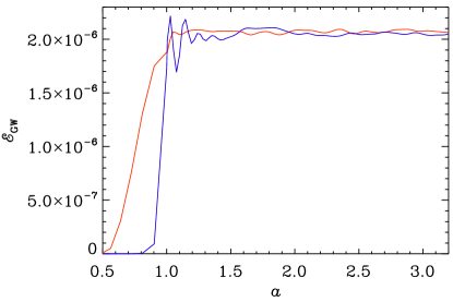
Figure 14: Comparison of ${\cal E}_{\rm GW}(t)$ for a run with quenching (red line) and without (blue).

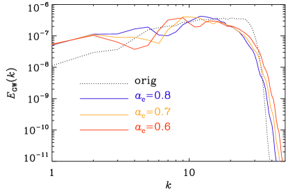
Figure 15: GW energy spectra for different values of $a_{\rm c}$, compared with the original Run D2 of Brandenburg et al. (2021d).

In Figure 15, we show GW spectra for different values of $a_{\rm c}$. We see that the effect of quenching is to make the spectra somewhat shallower. This suggests that a correspondence between the stress spectra and the spectra of GW energy can only be reached when the rapid growth of GW energy has come to an end. Denoting the computation of spectra again by an operator Sp, we can say that $\mbox{\rm Sp}(T)\approx\mbox{\rm Sp}(k^{2}\tilde{h})=k^{2}\mbox{\rm Sp}(k\tilde{h})=E_{\rm GW}(k)$, which agrees with our findings. Thus, in conclusion, the change from a $k^{1}$ spectrum to $k^{0}$ found in the simulations of Brandenburg et al. (2021d) occurs when the growth of electromagnetic energy has stopped. This is when $f^{\prime}=f^{\prime\prime}=0$, but it is not a direct consequence of the discontinuity at $\eta=1$ and therefore not an artifact.

References

- Ackermann et al. (2018) Ackermann, M., Ajello, M., Baldini, L., et al. 2018, The Astrophysical Journal Supplement Series, 237, 32, doi: 10.3847/1538-4365/aacdf7
- Adshead et al. (2020a) Adshead, P., Giblin, J. T., Pieroni, M., & Weiner, Z. J. 2020a, Phys. Rev. Lett., 124, 171301, doi: 10.1103/PhysRevLett.124.171301
- Adshead et al. (2020b) —. 2020b, Phys. Rev. D, 101, 083534, doi: 10.1103/PhysRevD.101.083534
- Adshead et al. (2016) Adshead, P., Giblin, J. T., Scully, T. R., & Sfakianakis, E. I. 2016, Journal of Cosmology and Astroparticle Physics, 2016, 039, doi: 10.1088/1475-7516/2016/10/039
- Amaro-Seoane et al. (2017) Amaro-Seoane, P., Audley, H., Babak, S., et al. 2017, arXiv e-prints, arXiv:1702.00786. https://arxiv.org/abs/1702.00786
- Anand et al. (2019) Anand, S., Bhatt, J. R., & Pandey, A. K. 2019, Eur. Phys. J. C, 79, 119, doi: 10.1140/epjc/s10052-019-6619-5
- Anber & Sorbo (2006) Anber, M. M., & Sorbo, L. 2006, J. Cosmology Astropart. Phys, 2006, 018, doi: 10.1088/1475-7516/2006/10/018
- Archambault et al. (2017) Archambault, S., Archer, A., Benbow, W., et al. 2017, The Astrophysical Journal, 835, 288, doi: 10.3847/1538-4357/835/2/288
- Arzoumanian et al. (2020) Arzoumanian, Z., Baker, P. T., Blumer, H., et al. 2020, ApJ, 905, L34, doi: 10.3847/2041-8213/abd401
- Bamba & Sasaki (2007) Bamba, K., & Sasaki, M. 2007, Journal of Cosmology and Astroparticle Physics, 2007, 030, doi: 10.1088/1475-7516/2007/02/030
- Bhatt & Pandey (2016) Bhatt, J. R., & Pandey, A. K. 2016, Phys. Rev. D, 94, 043536, doi: 10.1103/PhysRevD.94.043536
- Brandenburg (2018) Brandenburg, A. 2018, Pencil Code, v2018.12.16, Zenodo, doi: 10.5281/zenodo.2315093
- Brandenburg et al. (2021a) Brandenburg, A., Clarke, E., He, Y., & Kahniashvili, T. 2021a, PhRvD, in press, arXiv:2102.12428. https://arxiv.org/abs/2102.12428
- Brandenburg et al. (1996) Brandenburg, A., Enqvist, K., & Olesen, P. 1996, Phys. Rev. D, 54, 1291, doi: 10.1103/PhysRevD.54.1291
- Brandenburg et al. (2021b) Brandenburg, A., Gogoberidze, G., Kahniashvili, T., et al. 2021b, Class. Quantum Grav., 38, 145002. https://arxiv.org/abs/2103.01140
- Brandenburg et al. (2021c) Brandenburg, A., He, Y., Kahniashvili, T., Rheinhardt, M., & Schober, J. 2021c, ApJ, 911, 110, doi: 10.3847/1538-4357/abe4d7
- Brandenburg et al. (2021d) Brandenburg, A., He, Y., & Sharma, R. 2021d, http://www.nordita.org/preprints, no. 2021-063
- Brandenburg & Kahniashvili (2017) Brandenburg, A., & Kahniashvili, T. 2017, Phys. Rev. Lett., 118, 055102, doi: 10.1103/PhysRevLett.118.055102
- Brandenburg et al. (2017) Brandenburg, A., Kahniashvili, T., Mandal, S., et al. 2017, Phys. Rev. D, 96, 123528, doi: 10.1103/PhysRevD.96.123528
- Brandenburg et al. (2015) Brandenburg, A., Kahniashvili, T., & Tevzadze, A. G. 2015, Phys. Rev. Lett., 114, 075001, doi: 10.1103/PhysRevLett.114.075001
- Campanelli (2009) Campanelli, L. 2009, Int. J. Mod. Phys. D, 18, 1395, doi: 10.1142/S0218271809015175
- Caprini & Durrer (2006) Caprini, C., & Durrer, R. 2006, Phys. Rev., D74, 063521, doi: 10.1103/PhysRevD.74.063521
- Caprini & Figueroa (2018) Caprini, C., & Figueroa, D. G. 2018, Classical and Quantum Gravity, 35, 163001, doi: 10.1088/1361-6382/aac608
- Caprini & Sorbo (2014) Caprini, C., & Sorbo, L. 2014, J. Cosmology Astropart. Phys, 2014, 056, doi: 10.1088/1475-7516/2014/10/056
- Caprini et al. (2016) Caprini, C., Hindmarsh, M., Huber, S., et al. 2016, J. Cosmology Astropart. Phys, 2016, 001, doi: 10.1088/1475-7516/2016/04/001
- Cornwall (1997) Cornwall, J. M. 1997, Phys. Rev. D, 56, 6146, doi: 10.1103/PhysRevD.56.6146
- Demozzi et al. (2009) Demozzi, V., Mukhanov, V., & Rubinstein, H. 2009, Journal of Cosmology and Astroparticle Physics, 8, 025, doi: 10.1088/1475-7516/2009/08/025
- Dolgov (1993) Dolgov, A. D. 1993, Phys. Rev. D, 48, 2499, doi: 10.1103/PhysRevD.48.2499
- Dolgov et al. (2002) Dolgov, A. D., Grasso, D., & Nicolis, A. 2002, Phys. Rev. D, 66, 103505, doi: 10.1103/PhysRevD.66.103505
- Durrer et al. (2011) Durrer, R., Hollenstein, L., & Jain, R. K. 2011, JCAP, 1103, 037, doi: 10.1088/1475-7516/2011/03/037
- Ellis et al. (2019) Ellis, J., Lewicki, M., & No, J. M. 2019, Journal of Cosmology and Astroparticle Physics, 2019, 003, doi: 10.1088/1475-7516/2019/04/003
- Ellis et al. (2020) Ellis, J., Lewicki, M., & Vaskonen, V. 2020, Journal of Cosmology and Astroparticle Physics, 2020, 020, doi: 10.1088/1475-7516/2020/11/020
- Ferreira et al. (2013) Ferreira, R. J. Z., Jain, R. K., & Sloth, M. S. 2013, J. Cosmology Astropart. Phys, 2013, 004, doi: 10.1088/1475-7516/2013/10/004
- Field & Carroll (2000) Field, G. B., & Carroll, S. M. 2000, Phys. Rev. D, 62, 103008, doi: 10.1103/PhysRevD.62.103008
- Fischler et al. (1985) Fischler, W., Ratra, B., & Susskind, L. 1985, Nuclear Physics B, 259, 730, doi: 10.1016/0550-3213(85)90011-2
- Fujita & Durrer (2019) Fujita, T., & Durrer, R. 2019, Journal of Cosmology and Astroparticle Physics, 2019, 008, doi: 10.1088/1475-7516/2019/09/008
- Fujita et al. (2015) Fujita, T., Namba, R., Tada, Y., Takeda, N., & Tashiro, H. 2015, Journal of Cosmology and Astroparticle Physics, 2015, 054, doi: 10.1088/1475-7516/2015/05/054
- Garretson et al. (1992) Garretson, W. D., Field, G. B., & Carroll, S. M. 1992, Phys. Rev. D, 46, 5346, doi: 10.1103/PhysRevD.46.5346
- Gogoberidze et al. (2007) Gogoberidze, G., Kahniashvili, T., & Kosowsky, A. 2007, Phys. Rev. D, 76, 083002, doi: 10.1103/PhysRevD.76.083002
- He et al. (2021) He, Y., Brandenburg, A., & Sinha, A. 2021, JCAP, 07, 015. https://arxiv.org/abs/2104.03192
- Hindmarsh et al. (2015) Hindmarsh, M., Huber, S. J., Rummukainen, K., & Weir, D. J. 2015, Phys. Rev. D, 92, 123009, doi: 10.1103/PhysRevD.92.123009
- Hindmarsh et al. (2017) —. 2017, Phys. Rev. D, 96, 103520, doi: 10.1103/PhysRevD.96.103520
- Joyce & Shaposhnikov (1997) Joyce, M., & Shaposhnikov, M. 1997, Phys. Rev. Lett., 79, 1193, doi: 10.1103/PhysRevLett.79.1193
- Kahniashvili et al. (2012) Kahniashvili, T., Brandenburg, A., Campanelli, L., Ratra, B., & Tevzadze, A. G. 2012, Phys. Rev. D, 86, 103005, doi: 10.1103/PhysRevD.86.103005
- Kahniashvili et al. (2017) Kahniashvili, T., Brandenburg, A., Durrer, R., Tevzadze, A. G., & Yin, W. 2017, J. Cosm. Astro-Part. Phys., 2017, 002, doi: 10.1088/1475-7516/2017/12/002
- Kahniashvili et al. (2021) Kahniashvili, T., Brandenburg, A., Gogoberidze, G., Mandal, S., & Pol, A. R. 2021, Phys. Rev. Res., 3, 013193, doi: 10.1103/PhysRevResearch.3.013193
- Kahniashvili et al. (2005) Kahniashvili, T., Gogoberidze, G., & Ratra, B. 2005, Phys. Rev. Lett., 95, 151301, doi: 10.1103/PhysRevLett.95.151301
- Kahniashvili et al. (2010) Kahniashvili, T., Kisslinger, L., & Stevens, T. 2010, Phys. Rev. D, 81, 023004, doi: 10.1103/PhysRevD.81.023004
- Kahniashvili et al. (2008) Kahniashvili, T., Kosowsky, A., Gogoberidze, G., & Maravin, Y. 2008, Phys. Rev. D, 78, 043003, doi: 10.1103/PhysRevD.78.043003
- Kamionkowski et al. (1994) Kamionkowski, M., Kosowsky, A., & Turner, M. S. 1994, Phys. Rev. D, 49, 2837, doi: 10.1103/PhysRevD.49.2837
- Kisslinger et al. (2005) Kisslinger, L. S., Walawalkar, S., & Johnson, M. B. 2005, Phys. Rev. D, 71, 065017, doi: 10.1103/PhysRevD.71.065017
- Kobayashi (2014) Kobayashi, T. 2014, J. Cosmology Astropart. Phys, 2014, 040, doi: 10.1088/1475-7516/2014/05/040
- Kobayashi & Afshordi (2014) Kobayashi, T., & Afshordi, N. 2014, Journal of High Energy Physics, 2014, 166, doi: 10.1007/JHEP10(2014)166
- Kobayashi & Sloth (2019) Kobayashi, T., & Sloth, M. S. 2019, Phys. Rev. D, 100, 023524, doi: 10.1103/PhysRevD.100.023524
- Kosowsky et al. (2002) Kosowsky, A., Mack, A., & Kahniashvili, T. 2002, Phys. Rev. D, 66, 024030, doi: 10.1103/PhysRevD.66.024030
- Kosowsky et al. (2002) Kosowsky, A., Mack, A., & Kahniashvili, T. 2002, Phys. Rev. D, 66, 024030, doi: 10.1103/PhysRevD.66.024030
- Kosowsky et al. (1992) Kosowsky, A., Turner, M. S., & Watkins, R. 1992, Phys. Rev. D, 45, 4514, doi: 10.1103/PhysRevD.45.4514
- Martin & Yokoyama (2008) Martin, J., & Yokoyama, J. 2008, Journal of Cosmology and Astroparticle Physics, 1, 025, doi: 10.1088/1475-7516/2008/01/025
- Miniati et al. (2018) Miniati, F., Gregori, G., Reville, B., & Sarkar, S. 2018, Phys. Rev. Lett., 121, 021301, doi: 10.1103/PhysRevLett.121.021301
- Namba et al. (2016) Namba, R., Peloso, M., Shiraishi, M., Sorbo, L., & Unal, C. 2016, Journal of Cosmology and Astroparticle Physics, 2016, 041, doi: 10.1088/1475-7516/2016/01/041
- Neronov et al. (2021) Neronov, A., Pol, A. R., Caprini, C., & Semikoz, D. 2021, Phys. Rev. D, 103, L041302, doi: 10.1103/PhysRevD.103.L041302
- Neronov & Vovk (2010) Neronov, A., & Vovk, I. 2010, Science, 328, 73, doi: 10.1126/science.1184192
- Nicolis (2004) Nicolis, A. 2004, Classical and Quantum Gravity, 21, L27, doi: 10.1088/0264-9381/21/4/l05
- Niksa et al. (2018) Niksa, P., Schlederer, M., & Sigl, G. 2018, Class. Quant. Grav., 35, 144001, doi: 10.1088/1361-6382/aac89c
- Okano & Fujita (2021) Okano, S., & Fujita, T. 2021, J. Cosmology Astropart. Phys, 2021, 026, doi: 10.1088/1475-7516/2021/03/026
- Pencil Code Collaboration et al. (2021) Pencil Code Collaboration, Brandenburg, A., Johansen, A., et al. 2021, The Journal of Open Source Software, 6, 2807, doi: 10.21105/joss.02807
- Quashnock et al. (1989) Quashnock, J. M., Loeb, A., & Spergel, D. N. 1989, ApJ, 344, L49, doi: 10.1086/185528
- Ratra (1992) Ratra, B. 1992, ApJ, 391, L1, doi: 10.1086/186384
- Roper Pol et al. (2020a) Roper Pol, A., Brandenburg, A., Kahniashvili, T., Kosowsky, A., & Mandal, S. 2020a, Geophys. Astrophys. Fluid Dynam., 114, 130, doi: 10.1080/03091929.2019.1653460
- Roper Pol et al. (2020b) Roper Pol, A., Mandal, S., Brandenburg, A., Kahniashvili, T., & Kosowsky, A. 2020b, Phys. Rev. D, 102, 083512, doi: 10.1103/PhysRevD.102.083512
- Sharma (2021) Sharma, R. 2021, arXiv e-prints, arXiv:2102.09358. https://arxiv.org/abs/2102.09358
- Sharma et al. (2017) Sharma, R., Jagannathan, S., Seshadri, T. R., & Subramanian, K. 2017, Phys. Rev. D, 96, 083511, doi: 10.1103/PhysRevD.96.083511
- Sharma et al. (2018) Sharma, R., Subramanian, K., & Seshadri, T. R. 2018, Phys. Rev. D, 97, 083503, doi: 10.1103/PhysRevD.97.083503
- Sharma et al. (2020) —. 2020, Phys. Rev. D, 101, 103526, doi: 10.1103/PhysRevD.101.103526
- Sigl et al. (1997) Sigl, G., Olinto, A. V., & Jedamzik, K. 1997, Phys. Rev. D, 55, 4582, doi: 10.1103/PhysRevD.55.4582
- Sobol et al. (2019) Sobol, O. O., Gorbar, E. V., & Vilchinskii, S. I. 2019, Phys. Rev. D, 100, 063523, doi: 10.1103/PhysRevD.100.063523
- Subramanian (2010) Subramanian, K. 2010, Astronomische Nachrichten, 331, 110, doi: 10.1002/asna.200911312
- Taiji Scientific Collaboration et al. (2021) Taiji Scientific Collaboration, Wu, Y.-L., Luo, Z.-R., Wang, J.-Y., et al. 2021, Communications Physics, 4, 34, doi: 10.1038/s42005-021-00529-z
- Tavecchio et al. (2011) Tavecchio, F., Ghisellini, G., Bonnoli, G., & Foschini, L. 2011, Monthly Notices of the Royal Astronomical Society, 414, 3566, doi: 10.1111/j.1365-2966.2011.18657.x
- Taylor et al. (2011) Taylor, A. M., Vovk, I., & Neronov, A. 2011, Astron. Astrophys., 529, A144, doi: 10.1051/0004-6361/201116441
- Tevzadze et al. (2012) Tevzadze, A. G., Kisslinger, L., Brandenburg, A., & Kahniashvili, T. 2012, The Astrophysical Journal, 759, 54, doi: 10.1088/0004-637x/759/1/54
- Turner & Widrow (1988) Turner, M. S., & Widrow, L. M. 1988, Phys. Rev. D, 37, 2743, doi: 10.1103/PhysRevD.37.2743
- Vilenkin (1980) Vilenkin, A. 1980, Phys. Rev. D, 22, 3080, doi: 10.1103/PhysRevD.22.3080
- Zrake (2014) Zrake, J. 2014, ApJ, 794, L26, doi: 10.1088/2041-8205/794/2/L26