DisTop: Discovering a Topological representation to learn diverse and rewarding skills

Abstract

The optimal way for a deep reinforcement learning (DRL) agent to explore is to learn a set of skills that achieves a uniform distribution of states. Following this, we introduce DisTop, a new model that simultaneously learns diverse skills and focuses on improving rewarding skills. DisTop progressively builds a discrete topology of the environment using an unsupervised contrastive loss, a growing network and a goal-conditioned policy. Using this topology, a state-independent hierarchical policy can select where the agent has to keep discovering skills in the state space. In turn, the newly visited states allows an improved learnt representation and the learning loop continues. Our experiments emphasize that DisTop is agnostic to the ground state representation and that the agent can discover the topology of its environment whether the states are high-dimensional binary data, images, or proprioceptive inputs. We demonstrate that this paradigm is competitive on MuJoCo benchmarks with state-of-the-art algorithms on both single-task dense rewards and diverse skill discovery. By combining these two aspects, we show that DisTop achieves state-of-the-art performance in comparison with hierarchical reinforcement learning (HRL) when rewards are sparse. We believe DisTop opens new perspectives by showing that bottom-up skill discovery combined with representation learning can unlock the exploration challenge in DRL.

1 Introduction

In reinforcement learning (RL), an autonomous agent learns to solve a task by interacting with its environment [57] thus receiving a reward that has to be hand-engineered by an expert to efficiently guide the agent. However, when the reward is sparse or not available, the agent keeps having an erratic behavior.

This issue partially motivated methods where an agent hierarchically commits to a temporally extended behavior named skills [4] or options [58], thus avoiding erratic behaviors and easing the exploration of the environment [39, 3]. While it is possible to learn hierarchical skills with an extrinsic (i.e task-specific) reward [5, 51], it does not fully address the exploration issue. In contrast, if an agent learns skills in a bottom-up way with intrinsic rewards, it makes the skills task-independent [3]: they are learnt without access to an extrinsic reward. It follows that, to explore without extrinsic rewards, the intrinsic objective of an agent may be to acquire a large and diverse repertoire of skills. Such paradigm contrasts with the way prediction-based [12] or count-based [7] methods explore [3] since their inability to return to the frontier of their knowledge can make their exploration collapse [19]. Previous approaches [44, 50, 21] manage to learn a large set of different skills, yet they are learnt during a developmental period [41], which is just an unsupervised pre-training phase.

These approaches based on a pre-training phase are incompatible with a continual learning framework where the agent has to discover increasingly complex skills according to sequentially given tasks [56, 48]. Ideally, a continually learning agent should learn new diverse skills by default, and focus on extrinsically rewarding skills when it gets extrinsic rewards [49, 4]. It would make exploration very efficient since diverse skill learning can maximize the state entropy [29, 50]. To follow such principle, we assume that the agent should not focus on what to learn, as commonly done in RL, but rather on where to learn in its environment. Thus the agent should learn a representation that keeps the structure of the environment to be able to select where it is worth learning, instead of learning a representation that fits a wanted behavior which is most of the time unknown.

In this paper, we introduce a new way to learn a goal space and select the goals, keeping the learning process end-to-end. We propose a new model that progressively Discovers a Topological representation (DisTop) of the environment. DisTop bridges the gap between acquiring skills that reach a uniform distribution of embedded states, and solving a task. It makes diversity-based skill learning suitable for end-to-end exploration in a single-task setting irrespective of the ground state space. DisTop simultaneously optimizes three components: 1- it learns a continuous representation of its states using a contrastive loss that brings together consecutive states; 2- this representation allows the building of a discrete topology of the environment with a new variation of a Growing When Required network [40]. Using the clusters of the topology, DisTop can sample from an almost-arbitrary distribution of visited embedded states, without approximating the high-dimensional ground state distribution; 3- it trains a goal-conditioned deep RL policy to reach embedded states. Upon these 3 components, a hierarchical state-independent Boltzmann policy selects the cluster of skills to improve according to an extrinsic reward and a diversity-based intrinsic reward.

We show, through DisTop, that the paradigm of choosing where to learn in a learnt topological representation is more generic than previous approaches. Our contribution is 4-folds: 1- we visualize the representation learnt by DisTop and exhibit that, unlike previous approaches [50], DisTop is agnostic to the shape of the ground state space and works with states being images, high-dimensional proprioceptive data or high-dimensional binary data; 2- we demonstrate that DisTop  clearly outperforms ELSIM, a recent method that shares similar properties [4]; 3- we show that DisTop achieves similar performance with state-of-the-art (SOTA) algorithms on both single-task dense rewards settings [27] and multi-skills learning benchmarks [50]; 4- we show that it improves exploration over state-of-the-art hierarchical methods on hard hierarchical benchmarks.

2 Background

2.1 Goal-conditioned reinforcement learning for skill discovery

In episodic RL, the problem is modelled with a Markov Decision Process (MDP). An agent can interact with an unknown environment in the following way: the agent gets a state $s_{0}\in S$ that follows an initial state distribution $\rho_{0}(s)$. Its policy $\pi$ selects actions $a\in A$ to execute depending on its current state $s\in S$, $a_{execute}\sim\pi(a|s)$. Then, a new state is returned according to transition dynamics distribution $s^{\prime}\sim p(s^{\prime}|s,a)$. The agent repeats the procedure until it reaches a particular state or exceeds a fixed number of steps $T$. This loop is called an episode. An agent tries to adapt $\pi$ to maximize the expected cumulative discounted reward $\operatorname*{\mathbb{E}}_{\pi}\big{[}\sum_{t=0}^{T}\gamma^{t}R(s_{t-1},a_{t-1},s_{t})\big{]}$ where $\gamma$ is the discount factor. The policy $\pi_{\theta}$ can be approximated with a neural network parameterized by $\theta$ [27]. In our case, the agent tries to learn skills, defined as a policy that tries to target a state (which we name goal). To this end, it autonomously computes an intrinsic reward according to the chosen skill [3]. The intrinsic reward is approximated through parameters $\omega$. Following Universal Value Function Approximators [54], the intrinsic reward and the skill’s policy become dependent on the chosen goal $g$: $r_{t}^{g}=R_{\omega}(s_{t-1},a_{t-1},s_{t},g_{t})$ and $\pi_{\theta}^{g}(s)=\pi_{\theta}(s,g)$. Hindsight Experience Replay [2] is used to recompute the intrinsic reward to learn on arbitrary skills.

In particular, Skew-Fit [50] strives to learn goal-conditioned policies that visit a maximal entropy of states. To generate goal-states with high entropy, they learn a generative model that incrementally increases the entropy of generated goals and makes visited states progressively tend towards a uniform distribution. Assuming a parameterized generative model $q_{\psi}(s)$ is available, an agent would like to learn $\psi$ to maximize the log-likelihood of the state distribution according to a uniform distribution: $\operatorname*{\mathbb{E}}_{s\sim U(S)}\log q_{\psi}(s)$. But sampling from the uniform distribution $U(S)$ is hard since the set of reachable states is unknown. Skew-Fit uses importance sampling and approximates the true ratio with a skewed distribution of the generative model $q_{\psi}(s)^{\alpha_{skew}}$ where $\alpha_{skew}<0$. This way, it maximizes $\operatorname*{\mathbb{E}}_{s\sim Buffer}q_{\psi}(s)^{\alpha_{skew}}\log q_{\psi}(s)$ where $s$ are uniformly sampled from the buffer of the agent. $\alpha_{skew}$ defines the importance given to low-density states; if $\alpha_{skew}=0$, the distribution will stay similar, if $\alpha_{skew}=-1$, it strongly over-weights low-density states to approximate $U(S)$. In practice, they show that directly sampling states $s\sim\frac{1}{Z}q_{\psi}(s)^{\alpha_{skew}}$, with $Z$ being the normalization constant reduces the variance.

2.2 Contrastive learning and InfoNCE

Contrastive learning aims at discovering a similarity metric between data points [16]. First, positive pairs that represent similar data and fake negative pairs are built. Second they are given to an algorithm that computes a data representation able to discriminate the positive from the negative ones. InfoNCE [46] proposed to build positive pairs from states that belong to the same trajectory. The negative pairs are built with states randomly sampled. For a sampled trajectory, they build a set $S_{N}$ that concatenates $N-1$ negative states and a positive one $s_{t+p}$. Then, they maximize $\mathbb{L}_{InfoNCE}^{N}=-\operatorname*{\mathbb{E}}_{S_{N}}\big{[}\log\frac{f_{p}(s_{t+p},v_{t})}{\sum_{s_{j}\in S_{N}}f_{p}(s_{j},v_{t})}\big{]}$ where $v_{t}$ is a learnt aggregation of previous states, $p$ indicates the additional number of steps and $f_{p}$ is a positive similarity function. The numerator brings together states that are part of the same trajectory and the denominator pushes away negative pairs. InfoNCE maximizes a lower bound of the mutual information $I(c_{t},s_{t+k})$ where $I(X,Y)=D_{KL}(p(x,y)||p(x)p(y))$ defines the quantity of information that a random variable contains on another.

3 Method

We propose to redefine the interest of an agent so that its default behavior is to learn skills that achieve a uniform distribution of states while focusing its skill discovery in extrinsically rewarding areas when a task is provided. If the agent understands the true intrinsic environment structure and can execute the skills that navigate in the environment, a hierarchical policy would just have to select the state to target and to call for the corresponding skill. However, it is difficult to learn both skills and the structure. First the ground representation of states may give no clue of this structure and may be high-dimensional. Second, the agent has to autonomously discover new reachable states. Third, the agent must be able to easily sample goals where it wants to learn.

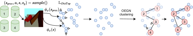
Figure 1: Illustration of a learning step of our growing network and contrastive loss (cf. text). Cylinders are buffers associated to each cluster, blue circles are states embedded with $\phi$ and pink circles represent clusters. The image is an example of state in the Visual Door[44] environment.

DisTop tackles theses challenges by executing skills that target low-density or previously rewarding visited states in a learnt topological representation. Figure 1 illustrates how DisTop learns a topological representation. It samples an interaction $(s_{prev},a,s,s_{g})$ from different buffers (see below), where $s_{g}$ is the original goal-state, and embeds the associated observations with a neural network $\phi_{\omega}$. Then, $\phi_{\omega}$ is trained with the contrastive loss that guarantees the proximity between consecutive states (cf. §3.1). After that, our growing network dynamically clusters the embedded states in order to uniformly cover the embedded state distribution. DisTop approximates the probability density of visiting a state with the probability of visiting its cluster (cf. §3.2). Then, it assigns buffers to clusters, and can sample goal-states or states with almost-arbitrary density over the support of visited states, e.g the uniform or reward-weighted ones (cf. §3.3).

At the beginning of each episode, a state-independent Boltzmann policy $\pi_{high}$ selects a cluster; then a state $s$ is selected that belongs to the buffer of the selected cluster and finally compute its representation $g=\phi_{\omega^{\prime}}(s)$ (see §3.3). A goal-conditioned policy $\pi_{\theta}^{g}$, trained to reach $g$, acts in the environment and discovers new reachable states close to its goal. The interactions made by the policy are stored in a buffer according to their initial objective and the embedding of the reached state.

3.1 Learning a representation with a metric

DisTop strives to learn a state representation $\phi_{\omega}$ that reflects the topology of its environment. We propose to maximize the constrained mutual information between the consecutive states resulting from the interactions of an agent. To do this, DisTop takes advantage of the InfoNCE loss (cf. §2.2). In contrast with previous approaches [38, 46, 37], we do not consider the whole sequence of interactions since this makes it more dependent on the policy. Typically, a constant and deterministic policy would lose the structure of the environment and could emerge once the agent has converged to an optimal deterministic policy. DisTop considers its local variant and builds positive pairs with only two consecutive states. This way, it keeps distinct the states that cannot be consecutive and it more accurately matches the topology of the environment. We propose to select our similarity function as $f_{\omega}(s_{t},s_{t+1})=e^{-k||\phi_{\omega}(s_{t})-\phi_{\omega}(s_{t+1})||_{2}}$ where $\phi_{\omega}$ is a neural network parameterized by $\omega$, $||_{2}$ is the L2 norm and $k$ is a temperature hyper-parameter [14]. If $\operatorname*{\mathbb{B}}$ is a batch of $N$ different consecutive pairs, the local InfoNCE objective, LInfoNCE, is described by eq. 1 (cf. Appendix C).

$$\mathbb{L}_{LInfoNCE} =\operatorname*{\mathbb{E}}_{(s_{t},s_{t+1})\in\operatorname*{\mathbb{B}}}\big{[}\log\frac{f_{\omega}(s_{t},s_{t+1})}{\sum_{s\in\operatorname*{\mathbb{B}}}f_{\omega}(s_{t},s)}\big{]}$$

$$\geq\operatorname*{\mathbb{E}}_{(s_{t},s_{t+1})\in\operatorname*{\mathbb{B}}}\big{[}-k||\phi_{\omega}(s_{t})-\phi_{\omega}(s_{t+1})||_{2}-\log(1+\sum_{s\in\operatorname*{\mathbb{B}}_{s\neq s_{t+1}}}f_{\omega}(s,s_{t+1}))\big{]}$$ (1)

We introduce the lower bound since it stabilizes the learning process. Intuitively, eq. 1 brings together states that are consecutive, and pushes away states that are separated by a large number of actions. This is illustrated in the second and third steps of Figure 1. There are several drawbacks with this objective function: the representation may be strongly distorted, making a clustering algorithm inefficient, and may be too unstable to be used by a DRL algorithm. To tackle this, eq. 2 reformulates the objective as a constrained maximization. Firstly, DisTop guarantees that the distance between consecutive states is below a threshold $\delta$ (first constraint of eq. 2). Secondly, it forces our representation to stay consistent over time (second constraint of eq. 2). Weights $\omega^{\prime}$ are a slow exponential moving average of $\omega$.

$$\max_{\omega}\quad\operatorname*{\mathbb{E}}_{(s_{t+1})\in\operatorname*{\mathbb{B}}}-\log(1+\sum_{s\in\operatorname*{\mathbb{B}}}f_{\omega}(s,s_{t+1}))\quad\textrm{s.t.} \quad\operatorname*{\mathbb{E}}_{(s_{t},s_{t+1})\in\operatorname*{\mathbb{B}}}||\phi_{\omega}(s_{t})-\phi_{\omega}(s_{t+1})||_{2}\geq\delta$$ (2)

$$\operatorname*{\mathbb{E}}_{s_{t+1}\in\operatorname*{\mathbb{B}}}||\phi_{\omega}(s_{t+1})-\phi_{\omega^{\prime}}(s_{t+1})||_{2}^{2}=0$$

Transforming the constraints into penalties, we get our final objective in eq. 3. $k_{c}$ is the temperature hyper-parameter that brings closer consecutive states, $\beta$ is the coefficient that slows down the speed of change of the representation.

$$\mathbb{L}_{DisTop~{}} =\operatorname*{\mathbb{E}}_{(s_{t},s_{t+1})\in\operatorname*{\mathbb{B}}}\big{[}-k_{c}(relu(||\phi_{\omega}(s_{t})-\phi_{\omega}(s_{t+1})||_{2}-\delta))-\log(1+\sum_{s\in\operatorname*{\mathbb{B}}}f_{\omega}(s,s_{t+1}))$$

$$+\beta||\phi_{\omega}(s_{t+1})-\phi_{\omega^{\prime}}(s_{t+1})||_{2}^{2}\big{]}$$ (3)

By applying this objective function, DisTop learns a consistent, not distorted representation that keeps close consecutive states while avoiding collapse (see Figure 2 for an example). In fact, by increasing $k_{c}$ and/or $k$, one can select the level of distortion of the representation (cf. Appendix A for an analysis). One can notice that the function depends on the distribution of consecutive states in $\operatorname*{\mathbb{B}}$; we experimentally found that using tuples $(s_{t},s_{t+1})$ from sufficiently stochastic policy is enough to keep the representation stable. We discuss the distribution of states that feed $\operatorname*{\mathbb{B}}$ in §3.4. In the following, we will study how DisTop takes advantage of this specific representation to sample diverse or rewarding state-goals.

3.2 Mapping the topology to efficiently sample rare states

In this section, we define the skewed distribution of goal-states, so that DisTop increases the entropy of visited states by over-sampling low-density goal-states. We propose to skew the sampling of visited states by partitioning the embedded space using a growing network; then we just need to weight the probability of sampling the partitions. It will promote sampling low-density goal-states (cf. §3.3) and will rule sampling for learning the goal-conditioned and the representation (cf. §3.4). We first give the working principle before explaining how we define the skewed distribution and sample from it.

Discovering the topology.

Since our representation strives to avoid distortion by keeping close consecutive states, DisTop can match the topology of the embedded environment by clustering the embedded states. DisTop uses an adaptation of a GWQ (cf. §B) called Off-policy Embedded Growing Network (OEGN). OEGN dynamically creates, moves and deletes clusters so that clusters generates a network that uniformly cover the whole set of embedded states, independently of their density; this is illustrated in the two last steps of Figure 1. Each node (or cluster) $c\in C$ has a reference vector $w_{c}$ which represents its position in the input space. The update operators make sure that all embedded states $s$ are within a ball centered on the center of its cluster, i.e $min_{c}\operatorname*{(\phi_{\omega}(s)-w_{c})^{\top}(\phi_{\omega}(s)-w_{c})}\leq\delta_{new}$ where $\delta_{new}$ is a threshold for creating clusters. $\delta_{new}$ is particularly important since it is responsible of the granularity of the clustering: if it is low, we will have a lot of small clusters, else we will obtain few large clusters that badly approximate the topology. The algorithm works as follows: assuming a new low-density embedded state is discovered, there are two possibilities: 1- the balls currently overlap: OEGN progressively moves the clusters closer to the new state and reduces overlapping; 2- the clusters almost do not overlap and OEGN creates a new cluster next to the embedded state. A learnt discrete topology can be visualized at the far right of Figure 2. Details about OEGN can be found in §B.

Sampling from a skewed distribution

To sample more often low-density embedded states, we assume that the density of a visited state is reflected by the marginal probability of its cluster. So we approximate the density of a state with the density parameterized by $w$, reference vector of $s$: $q_{w}(s)\approx\frac{count(c_{s})}{\sum_{c^{\prime}\in C}count(c^{\prime})}$ where $count(c_{s})$ is the number of states that belong to the cluster that contains $s$. Using this approximation, we skew the distribution very efficiently by first sampling a cluster with the probability given by $p_{\alpha_{skew}}(c)=\frac{count(c)^{1+\alpha_{skew}}}{\sum_{c^{\prime}\in C}count(c^{\prime})^{1+\alpha_{skew}}}$ where $\alpha_{skew}$ is the skewed parameter (cf. §2). Then we randomly sample a state that belongs to the cluster.

While our approximation $q_{w}(s)$ decreases the quality of our skewed objective, it makes our algorithm very efficient: we associate a buffer to each cluster and only weight the distribution of clusters; DisTop does not weight each visited state [50], but only a limited set of clusters. In practice we can trade-off the bias and the instability of OEGN by decreasing $\delta_{new}$: the smaller the clusters are, the smaller the bias is, but the more unstable is OEGN and the sampling distribution. So, in contrast with Skew-Fit, we do not need to compute the approximated density of each state, we just need to keep states in the buffer of their closest node. In practice, we associate to each node a second buffer that takes in interactions if the corresponding node is the closest to the interaction’s goal. This results in two sets of buffers: $\operatorname*{\mathbb{B}}^{G}$ and $B^{S}$ to sample state-goals and states, respectively, with the skewed distribution.

In the next sections, we will detail how we use this skewed distribution over $\operatorname*{\mathbb{B}}^{G}$ and $B^{S}$ for sampling low-density goal-states (§3.3) and sampling learning interactions (§3.4).

3.3 Selecting novel or rewarding skills

It is not easy to sample new reachable goals. For instance, using an embedding space $\mathbb{R}^{10}$, the topology of the environment may only exploit a small part of it, making most of the goals pointless. Similarly to previous works [60], DisTop generates goals by sampling previously visited states. To sample the states, DisTop first samples a cluster, and then samples a state that belongs to the cluster.

Sampling a cluster:

To increase the entropy of states, DisTop samples goal-states with the skewed distribution defined in §3.2 that can be reformulated as:

$$p_{\alpha_{skew}}(c) =\frac{e^{(1+\alpha_{skew})\log count(c)}}{\sum_{c^{\prime}\in C}e^{{(1+\alpha_{skew})\log count(c^{\prime})}}}$$ (4)

It is equivalent to sampling with a simple Boltzmann policy $\pi^{high}$, using a novelty bonus reward $\log count(c)$ and a fixed temperature parameter $1+\alpha_{skew}$. In practice, we can use a different $\alpha_{skew}^{\prime}$ than in §3.2 to trade-off the importance of the novelty reward in comparison with an extrinsic reward (see below) or decrease the speed at which we gather low-density states [50].

We can add a second reward to modify our skewed policy $\pi^{high}$ so as to take into consideration extrinsic rewards. We associate to a cluster $c\in C$ a value $r_{c}$ that represents the mean average extrinsic rewards received by the skills associated to its goals :

$$r_{c}=\operatorname*{\mathbb{E}}_{s\in c,g=\phi_{\omega}(s)}\frac{1}{T}\sum_{t=0}^{T}\operatorname*{\mathbb{E}}_{a_{t}\sim\pi_{\theta}^{g}(\cdot|s_{t}),s_{t+1}\sim p(\cdot|s_{t},a_{t})}R(s_{t},a_{t},s_{t+1}).$$ (5)

The extrinsic value of a cluster $R_{c}^{ext}$ is updated with an exponential moving average $R_{c}^{ext}=(1-\alpha_{c})*R_{c}^{ext}+\alpha_{c}*r_{c}$ where $\alpha_{c}$ is the learning rate. To favours exploration, we can also update the extrinsic value of the cluster’s neighbors with a slower learning rate (cf. Appendix D). Our sampling rule can then be :

$$\pi^{high}(c) =\text{softmax}_{C}(t^{ext}R_{c}^{ext}+(1+\alpha_{skew}^{\prime})\log count(c))$$ (6)

Sampling a state:

Once the cluster is selected, we keep exploring independently of the presence of extrinsic rewards. To approximate a uniform distribution over visited states that belongs to the cluster, DisTop samples a vector in the ball that surrounds the center of the cluster. It rejects the vector and samples another one if it does not belong to the cluster. Finally, it selects the closest embedded state to the vector.

3.4 Learning goal-conditioned policies

We now briefly introduce the few mechanisms used to efficiently learn the goal-conditioned policies. Once the goal-state $s_{g}$ is selected, the agent embeds it as $g=\phi_{\omega^{\prime}}(s_{g})$. It uses the target weights $\omega^{\prime}$ to make our goal-conditioned policy independent from fluctuations due to the learning process. In consequence, we avoid using a hand-engineered environment-specific scheduling [50]. Our implementation of the goal-conditioned policy is trained with Soft Actor-Critic (SAC)[27] and the reward is the L2 distance between the state and the goal in the learnt representation. In practice, our goal-conditioned policy $\pi_{\theta}$ needs a uniform distribution of goals to avoid forgetting previously learnt skills. Our representation function $\phi_{\omega}$ requires a uniform distribution over visited states to quickly learn the representation of novel areas. In consequence, DisTop samples a cluster $c\sim p_{\alpha_{skew}}$ and randomly takes half of the interactions from $\operatorname*{\mathbb{B}}^{G}$ and the rest from $\operatorname*{\mathbb{B}}^{S}$. We can also sample a ratio of clusters with $\pi^{high}$ if we do not care about forgetting skills (cf. Appendix A). $\theta$, $\omega$ and $w$ are learnt over the same mini-batch and we relabel the goals extracted from $\operatorname*{\mathbb{B}}^{S}$ (cf. Appendix D).

4 Experiments

Our experiments aim at emphasizing the genericity of DisTop. Firstly, unlike generative models in the ground state space, DisTop learns the true topology of the environment even though the ground state representation lacks structure. Secondly, when it does not access rewards, the discovered skills are as diverse as a SOTA algorithm (Skew-Fit [50]) on robotic arm environments using images. Thirdly, even though acquiring diverse skills may be useless, DisTop is still able to perform close to a SOTA algorithm (SAC [27]) in MuJoCo environments [59]. Finally, we compare DisTop with a SOTA hierarchical algorithm (LESSON [37]) in a sparse reward version of an agent that navigates in a maze [43]. All curves are a smooth averaged over 5 seeds, completed with a shaded area that represent the mean +/- the standard deviation over seeds. Used hyper-parameters are described in Appendix E, environments and evaluation protocols details are given in Appendix F. Videos and images are available in supplementary materials.

Is DisTop able to learn diverse skills without rewards ?

We assess the diversity of learnt skills on two robotic tasks Visual Pusher (a robotic arm moves in 2D and eventually pushes a puck) and Visual Door (a robotic arm moves in 3D and can open a door) [44]. We compare to Skew-Fit [50]. These environments are particularly challenging since the agent has to learn from 48x48 images using continuous actions. We use the same evaluation protocol than Skew-Fit: a set of images are sampled, given to the representation function and the goal-conditioned policy executes the skill. In Figure 3, we observe that skills of DisTop are learnt quicker on Visual Pusher but are slightly worst on Visual Door. Since the reward function is similar, we hypothesize that this is due to the structure of the learnt goal space. In practice we observed that DisTop is more stochastic than Skew-Fit since the intrinsic reward function is required to be smooth over consecutive states. Despite the stochasticity, it is able to reach the goal as evidenced by the minimal distance reached through the episode. Stochasticity does not bother evaluation on Visual Pusher since the arm moves elsewhere after pushing the puck in the right position.

Does DisTop discover the environment topology even though the ground state space is unstructured ?

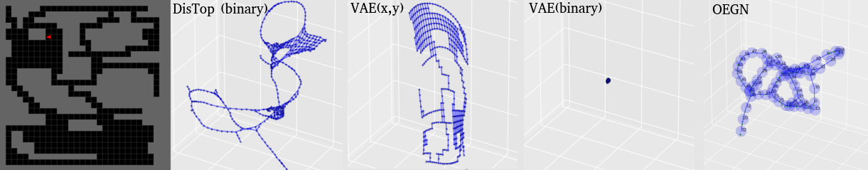
Figure 2: Visualization of the representations learnt by a VAE and DisTop. From left to right, we respectively see a- the rendering of the maze; b- the representation learnt by DisTop with 900-dimensional binary inputs; c- a VAE representation with true (x,y) coordinates; d- a VAE representation with 900-dimensional binary inputs; e- OEGN network learnt from binary inputs.

In this experiment, we analyze the representation learnt by a standard Variational Auto Encoder (VAE) and DisTop. To make sure that the best representation is visualizable, we adapted the gym-minigrid environment [15] (cf. Figure 2) where a randomly initialized agent moves for fifty timesteps in the four cardinal directions. Each observation is either a 900-dimensional one-hot vector with 1 at the position of the agent (binary) or the (x,y) coordinates of the agent. Interactions are given to the representation learning algorithm. Except for OEGN, we display as a node the learnt representation of each possible state and connect states that are reachable in one step. In Figure 2, we clearly see that DisTop is able to discover the topology of its environment since each connected points are distinct but close with each other. In contrast, the VAE representation collapses since it cannot take advantage of the proximity of states in the ground state space; it only learns a correct representation when it gets (x,y) positions, which are well-structured. This toy visualization highlights that, unlike VAE-based models, DisTop does not depend on well-structured ground state spaces to learn a suitable environment representation for learning skills.

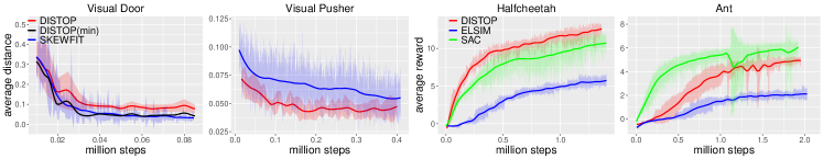
Figure 3: Left: Comparison of DisTop and Skew-Fit on their ability to reach diverse states. In the Visual Pusher environment, we compare the final distance of the position puck with its desired position; in the door environment, we compare the angle of the door with the desired angle. DisTop(min) is the minimal distance reached through evaluation episode. At each evaluation iteration, the distances are averaged over fifty goals. Right: Average rewards gathered throughout episodes of 300 steps while training on Halfcheetah-v2 and Ant-v2 environments.

Can DisTop solve non-hierarchical dense rewards tasks?

We test DisTop on MuJoCo environments Halfcheetah-v2 and Ant-v2 [59], the agent gets rewards to move forward as fast as possible. We fix the maximal number of timesteps to 300. We compare DisTop to our implementation of SAC[27] and to ELSIM [4], a method that follows the same paradigm than DisTop (see §5). We obtain better results than in the original ELSIM paper using similar hyper-parameters to DisTop. In Figure 3 (Right), we observe that DisTop obtains high extrinsic rewards and clearly outperforms ELSIM. It also outperforms SAC on Halfcheetah-v2, but SAC still learns faster on Ant-v2. We highlight that SAC is specific to dense rewards settings and cannot learn in sparse settings (see below).

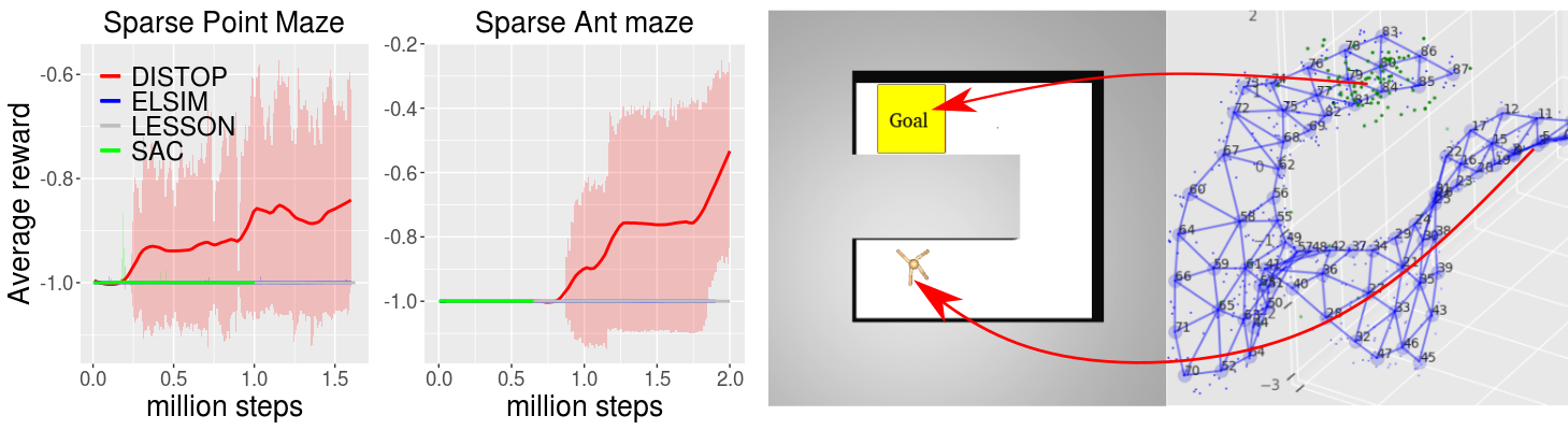
Figure 4: Left: Average rewards throughout training episodes. Right: Visualization of Ant Maze environment with its goal position and, to its right, an example of OEGN network learnt by DisTop. Small green points represent selected goal-states.

Does combining representation learning, entropy of states maximization and task-learning improve exploration on high-dimensional hierarchical tasks ?

We evaluate DisTop ability to explore and optimize rewards on image-based versions of Ant Maze and Point Maze environments [43]. The state is composed of a proprioceptive state of the agent and a top view of the maze ("Image"). In contrast with previous methods [43, 37], we remove the implicit curriculum that changes the extrinsic goal across episodes; here we train only on the farthest goal and use a sparse reward function. Thus, the agent gets a non-negative reward only when it gets close to the goal. We compare our method with a SOTA HRL method, LESSON [37] (see §5), ELSIM and our implementation of SAC [27]. For ELSIM, LESSON and DisTop, we only pass the "image" to the representation learning part of the algorithms, assuming that an agent can separate its proprioceptive state from the sensorial state. In Figure 4, we can see that DisTop is the only method that manages to return to the goal; in fact, looking at a learnt 3D OEGN network, we can see that it successfully represent the U-shape form of the maze and set goals close to the extrinsic goal. LESSON discovers the goal but does not learn to return to it; we hypothesize that its high-level policy takes too long to gather enough interactions to learn on and that it still requires too many random high-level actions to find the goal. Neither SAC, nor ELSIM find the reward. We suppose that the undirected width expansion of the tree of ELSIM does not maximize the state-entropy, making it spend too much time in useless areas and thus inefficient for exploration. We admit that DisTop has high variance, but we argue that it is more a credit assignment issue [58] due to the long-term reward than an exploration problem.

5 Related works

Intrinsic skills in hierarchical RL

Some works propose to learn hierarchical skills, but do not introduce a default behavior that maximizes the visited state entropy [29], limiting the ability of an agent to explore. For example, it is possible to learn skills that target a ground state or a change in the ground state space [43, 36]. These approaches do not generalize well with high-dimensional states. To address this, one may want to generate rewards with a learnt representation of goals.NOR [42] bounds the sub-optimality of such representation to solve a task and LESSON [37] uses a slow dynamic heuristic to learn the representation. In fact, it uses an InfoNCE-like objective function; this is similar to [38] which learns the representation during pre-training with random walks. DCO [30] generates options by approximating the second eigenfunction of the combinatorial graph Laplacian of the MDP. It extends previous works [39, 6] to continuous state spaces. Above-mentioned methods uses a hierarchical random walk to explore the environment, we have shown in §4 that DisTop explores quicker by maximizing the entropy of states in its topological representation.

Intrinsic motivation to learn diverse skills.

DisTop simultaneously learns skills, their goal representation, and which skill to train on. It contrasts with several methods that exclusively focus on selecting which skill to train on assuming a good goal representation is available [23, 17, 24, 62, 18]. They either select goals according to a curriculum defined with intermediate difficulty and the learning progress [47] or by imagining new language-based goals [18]. In addition, DisTop strives to learn either skills that are diverse or extrinsically rewarding. It differs from a set of prior methods that learn only diverse skills during a pre-training phase, preventing exploration for end-to-end learning. Some of them maximize the mutual information (MI) between a set of states and skills. Typically, DIAYN [21], VALOR [1] and SNN [22] learn a discrete set of skills, but hardly generalize over skills. It has been further extended to continuous set of skills, using a generative model [55] or successor features [28, 11]. In both case, directly maximizing this MI may incite the agent to focus only on simple skills [13]. DISCERN [60] maximizes the MI between a skill and the last state of an episode using a contrastive loss. Unlike us, they use the true goal to generate positive pairs and use a L2 distance over pixels to define a strategy that improves the diversity of skills. In addition, unlike VAE-based models, our method better scales to any ground state space (see §4). Typically, RIG [44] uses a VAE [31] to compute a goal representation before training the goal-conditioned policies. Using a VAE, it is possible to define a frontier with a reachability network, from which the agent should start stochastic exploration [10]; but the gradual extension of the frontier is not automatically discovered, unlike approaches that maximize the entropy of states (including DisTop). Skew-Fit [50] further extended RIG to improve the diversity of learnt skills by making the VAE over-weight low-density states. Unlike DisTop, it is unclear how Skew-Fit could target another distribution over states than a uniform one. Approaches based on learning progress (LP) have already been built over VAEs [33, 34]; we believe that DisTop could make use of LP to avoid distractors or further improve skill selection.

Skill discovery for end-to-end exploration.

Like DisTop, ELSIM [4] can discover diverse and rewarding skills in an end-to-end way. It builds a tree of skills and selects the branch to improve with extrinsic rewards. DisTop outperforms ELSIM for both dense and sparse-rewards settings (cf. §4). This end-to-end setting has also been experimented through multi-goal distribution matching [49, 35] where the agent tries to reduce the difference between the density of visited states and a given distribution (with high-density in rewarding areas). Yet, either they approximate a distribution over the ground state space [35] or assume a well-structured state representation [49]. Similar well-structured goal space is assumed when an agent maximizes the reward-weighted entropy of goals [63].

Dynamic-aware representations.

A set of RL methods try to learn a topological map without addressing the problem of discovering new and rewarding skills. Some methods [52, 53, 20] consider a topological map over direct observations, but to give flat intrinsic rewards or make planning possible. We emphasize that SFA-GWR-HRL [64] hierarchically takes advantage of a topological map built with two GWQ placed over two Slow Feature Analysis algorithms [61]; it is unclear whether it can be applied to other environments than their robotic setting. Functional dynamic-aware representations can be discovered by making the distance between two states match the expected difference of trajectories to go to the two states [26]; interestingly, they exhibit the interest of topological representations for HRL and propose to use a fix number of clusters to create goals. Previous work also showed that an active dynamic-aware search of independent factors can disentangle the controllable aspects of an environment [8].

6 Conclusion

We introduced a new model, DisTop, that simultaneously learns a topology of its environment and the skills that navigate into it. In particular, it concentrates the skill discovery on parts of the topology with low-density embedded states until it discovers an extrinsic reward. In contrast with previous approaches, there is no pre-training [49, 50], particular scheduling [50] or random walks [38, 10]. It avoids catastrophic forgetting, does not need a well-structured goal space [49] or dense rewards [37]. Throughout all the experiments, we have shown that DisTop is generic : it keeps working and learn a dynamic-aware representation in dense rewards setting, pixel-based skill discovery environments and hard sparse rewards settings. Yet, there are limitations and exciting perspectives: HRL [26] and planning based approaches [45] could both take advantage of the topology and make easier states discovery; Frontier-based exploration [10] could also be explored to reduce skill stochasticity. Disentangling the topology [9] and learning progress measures [33] could further improve the scalability of the approach. Finally, we argue that, by tackling the problem of unsupervised learning of both dynamic-aware representations and skills without adding constraints in comparison to standard RL, DisTop opens the path towards more human-like open-ended DRL agents.

Appendix A Ablation study

In this section, we study the impact of the different key hyper-parameters of DisTop. Except for paper results, we average the results over 3 random seeds. For visualizations based on the topology, the protocol is the same as the one described §4. In addition, we select the most viewable one among 3 learnt topologies; while we did not observe variance in our analysis through the seeds, the 3D angle of rotation can bother our perception of the topology.

Details about maze experiments.

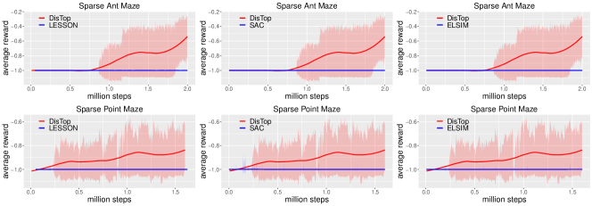
Figure 5: Same experiments than in §4.

Figure 5 shows the same experiments as in §4, but we duplicate the graph to clearly see the curves of each method. For SAC, we use different experiments with $\gamma=0.996$ rather than $\gamma=0.99$.

Controlling the distortion of the representation.

The analysis of our objective function $\mathbb{L}_{DisTop~{}}$ shares some similarities with standard works on contrastive learning [16]. However, we review it to clarify the role of the representation with respect to the interactions, the reward function and OEGN.

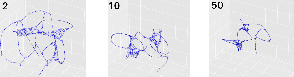
Figure 6: Different Topologies learnt on the gridworld displayed in §4. From left to right, we show the learnt topology with $k_{c}=2$, $k_{c}=10$, $k_{c}=50$.

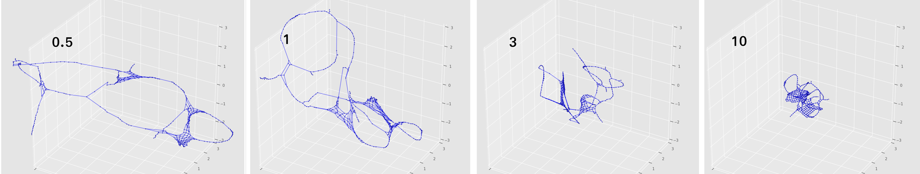
Figure 8: Different Topologies learnt on the gridworld displayed in §4. From left to right, we show the learnt topology with $k=0.5$, $k=1$, $k=3$, $k=10$.

In Figure 6, we can see that the distortion parameter $k_{c}$ rules the global dilatation of the learnt representation. A low $k_{c}$ also increases the distortion of the representation, which may hurt the quality of the clustering algorithm. $k_{c}$ is competing with $k$, the temperature hyper-parameter. As we can see in Figure 8, $k$ rules the minimal allowed distance between very different states. So that there is a trade-off between a low $k$ that distorts and makes the representation unstable, and a high $k$ that allows different states to be close with each other. With a high $k$, the L2 rewards may admit several local optimas.

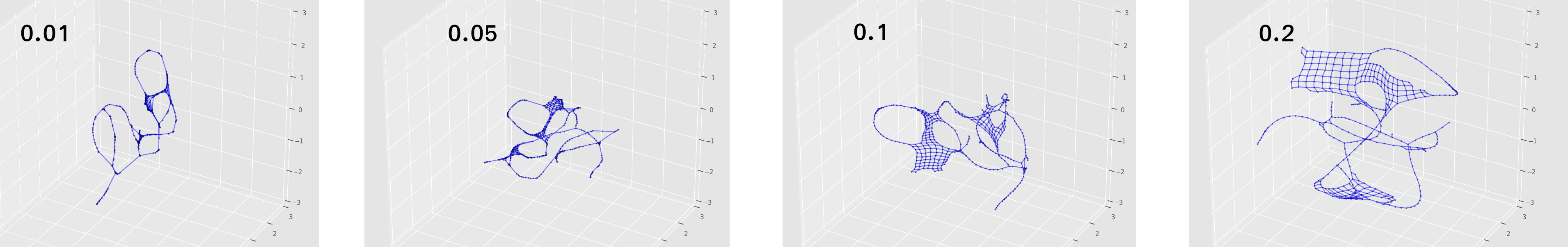
Figure 7: Different Topologies learnt on the gridworld displayed in §4. From left to right, we show the learnt topology with $\delta=0.01$, $\delta=0.05$, $\delta=0.1$, $\delta=0.2$.

In Figure 7, we see that $\delta$ also impacts the distortion of the representation, however it mostly limits the compression of the representation in the areas the agent often interacts in. In the borders, the agent often hurts the wall and stays in the same position. So in comparison with large rooms, the bring together is less important than the move away part. $\delta$ limits such asymmetries and keeps large rooms dilated. Overall, this asymmetry also occurs when the number of states increases due to the exploration of the agent: the agent progressively compresses its representation since interesting negative samples are less frequent.

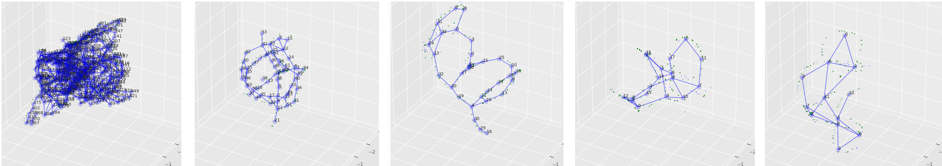
Figure 9: Different OEGN networks learnt according to $\delta_{new}$. From left to right, we show the OEGN network with $\delta_{new}=0.2$,$\delta_{new}=0.4$,$\delta_{new}=0.6$,$\delta_{new}=0.8$,$\delta_{new}=1$

The size of the clusters of OEGN has to match the distortion of the representation. Figure 9 emphasizes the importance of the creation threshold parameter $\delta_{new}$. If this is too low ($0.2$), clusters do not move and a lot of clusters are created. OEGN waits a long time to delete them. If it is too high, the approximation of the topology becomes very rough, and states that belong to very different parts of the topology are classified in the same cluster; this may hurt our density approximation.

Selection of interactions:

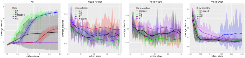
Figure 10: Different learning curves showing the impact of the choice of interactions. 1- We study the impact choosing learning interactions with $\pi^{high}$ rather than $p_{\alpha_{skew}}$. 2- we study the importance of $1+\alpha_{skew}^{\prime}$ in Visual Pusher. 3 and 4- we assess the importance of $1+\alpha_{skew}$ in Visual Pusher and Visual Door.

Figure 10 shows the importance of the different hyper-parameters that rule the sampling of goals and states. In Ant environment, we see that the agent has to sample a small ratio of learning interactions from $\pi^{high}$ rather than $p_{\alpha_{skew}}$; it speeds up its learning process by making it focus on important interactions. Otherwise, it is hard to learn all skills at the same time. However, the learning process becomes unstable if it deterministically samples from a very small set of clusters (ratios $0.9$ and $0.7$).

Then we evaluate the importance of $1+\alpha_{skew}^{\prime}$ on Visual Pusher. We see that the agent learns quicker with a low $1+\alpha_{skew}^{\prime}$. It hardly learns when the high-level policy almost does not over-sample low-density clusters ($-0.1$). This makes our results consistent with the analysis provided in the paper of Skew-Fit [50].

In the last two graphics of Figure 10, we show the impact of $1+\alpha_{skew}$; we observe that the agent learns quicker when $1+\alpha_{skew}$ is close to $0$. It highlights that the agent quicker learns both a good representation and novel skills by sampling uniformly over the clusters.

Overall, we also observe that some seeds become unstable. Since they coincide with large deletions of clusters. We expect that an hyper-parameter search on the delete operators of OEGN may solve this issue in these specific cases.

Appendix B OEGN and GWQ

Several methods introduced unsupervised neural networks to learn a discrete representation of a fixed input distribution [32, 25, 40]. The objective is to have clusters (or nodes) that cover the space defined by the input points. Each node $c\in C$ has a reference vector $w_{c}$ which represents its position in the input space. We are interested in the Growing when required algorithm (GWQ) [40] since it updates the structure of the network (creation and deletion of edges and nodes) and does not impose a frequency of node addition. OEGN is an adaptation of GWQ; algorithm 1 describes the core of these algorithms and their specific operators are described below. Specific operations of OEGN are colored in red, the ones of GWQ in blue and the common parts are black. Our modifications are made to 1- make the network aware of the dynamics; 2- adapt the network to the dynamically changing true distribution.

Delete operator:

Delete $node_{i}$ if $node_{i}.error$ is above a threshold $\delta_{error}$ to verify that the node is still active; delete the less filled neighbors of two neighbors if their distance is below $\delta_{prox}$ to avoid too much overlapping; check it has been selected $n_{del}$ times before deleting it. Delete if a node does not have edges anymore.

Both creation and moving operators:

Check that the distance between the original goal and the resulting embedding $||goal_{i}-e_{i}||_{2}$ is below a threshold $\delta_{success}$.

Creation operator:

Check if $||closest-e_{i}||_{2}>\delta_{new}$. Verify $closest$ has already been selected $\delta_{count}$ times by $\pi^{high}$. If the conditions are filled, a new node is created at the position of the incoming input $e_{i}$ and it is connected to $closest$. Update a firing count of the winning node and its neighbors and check it is below a threshold. A node is created halfway between the winning node and the second closest node. The two winning nodes are connected to the new node.

Moving operator:

If no node is created or deleted, which happens most of the time, we apply the moving operator described by eq. 7 assuming $closest=\operatorname*{argmin}_{c}(\phi_{\omega^{\prime}}(s)-w_{c})^{\top}(\phi_{\omega^{\prime}}(s)-w_{c})$. In our case, we use a very low $\alpha_{neighbors}$ to avoid the nodes to concentrate close to high-density areas.

$$w_{j}=\begin{cases}w_{j}+\alpha(\phi_{\omega^{\prime}}(s)-w_{j}),&\text{if $j=closest$}\\ w_{j}+\alpha_{neighbors}(\phi_{\omega^{\prime}}(s)-w_{j}),&\text{if $j\in neighbors(closest)$}\\ w_{j},&\text{otherwise.}\end{cases}$$ (7)

Edge operator:

edges are added or updated with attribute $age=0$ between the winning node of $e_{i}$ and the one of $e_{i}^{prev}$. Edges with $age=0$ are added or updated between the two closest nodes of $e_{i}$. When an edge is added or updated, increment the age of the other neighbors of $closest$ and delete edges that are above a threshold $\delta_{age}$.

Initialize network with two random nodes, set theirs attributes to 0 and connect them.

for each learning iteration do

     Sample a tuple $s_{i},node_{i},s_{i}^{prev}\leftarrow sample(\operatorname*{\mathbb{B}})$.

     Embed states: $e_{i}\leftarrow\phi_{\omega^{\prime}}(s_{i})$; $e_{i}^{prev}\leftarrow\phi_{\omega^{\prime}}(s_{i}^{prev})$

     Sample an input $e_{i}\leftarrow sample(\operatorname*{\mathbb{B}})$.

     $closest\leftarrow min_{nodes}(||nodes-e_{i}||_{2})$.

     Increase error count of $node_{i}$ by 1.

     Reset error count of $closest$ to 0

     Apply $DeleteOperator()$.

     If a node is deleted, stop the learning iteration

     Apply $CreationOperator()$.

     Apply $MovingOperator()$.

     Apply $EdgeOperator()$.

end for

Algorithm 1 Algorithm of OEGN (red) and GWQ (blue)

Except for $\delta_{new}$ and $\delta_{success}$, we emphasize that thresholds parameters have not been fine-tuned and are common to all experiments; we give them in Table 1.

Parameters	Value
Age deletion threshold $\delta_{age}$	$600$
Error deletion count $\delta_{error}$	$600$
Proximity deletion threshold $\delta_{prox}$	$0.4\times\delta_{new}$
Count creation threshold $\delta_{count}$	$5$
Minimal number of selection $n_{del}$	$10$
Learning rate $\alpha$	$0.001$
Neighbors learning rate $\alpha_{neighbors}$	$0.000001$
Number of updates per batch	$\sim 32$

Table 1: Fixed hyper-parameters used in OEGN. They have not been tuned.

Appendix C Derivation of the contrastive loss

$$\mathbb{L}_{InfoNCE} =\operatorname*{\mathbb{E}}_{(s_{t},s_{t+1})\in\operatorname*{\mathbb{B}}}\big{[}\log\frac{f_{\omega}(s_{t},s_{t+1})}{\sum_{s\in\operatorname*{\mathbb{B}}}f_{\omega}(s,s_{t+1})}\big{]}$$

$$=\operatorname*{\mathbb{E}}_{(s_{t},s_{t+1})\in\operatorname*{\mathbb{B}}}\big{[}-k||\phi_{\omega}(s_{t})-\phi_{\omega}(s_{t+1})||_{2}-\log(\sum_{s\in\operatorname*{\mathbb{B}}}f_{\omega}(s,s_{t+1}))\big{]}$$ (8)

$$=\operatorname*{\mathbb{E}}_{(s_{t},s_{t+1})\in\operatorname*{\mathbb{B}}}\big{[}-k||\phi_{\omega}(s_{t})-\phi_{\omega}(s_{t+1})||_{2}-\log(f_{\omega}(s_{t},s_{t+1})+\sum_{s\in\operatorname*{\mathbb{B}}_{s\neq s_{t}}}f(s,s_{t+1}))\big{]}$$ (9)

$$\geq\operatorname*{\mathbb{E}}_{(s_{t},s_{t+1})\in\operatorname*{\mathbb{B}}}\big{[}-k||\phi_{\omega}(s_{t})-\phi_{\omega}(s_{t+1})||_{2}-\log(1+\sum_{s\in\operatorname*{\mathbb{B}}_{s\neq s_{t}}}f(s,s_{t+1}))\big{]}$$ (10)

In the last line of eq. 10, we upper-bound $f_{\omega}(s_{t},s_{t+1})$ with 1 since $e^{-v}<1$ when $v$ is positive. The logarithmic function is monotonic, so the negative logarithm inverses the bound.

Appendix D Implementation details

In this section, we provide some details about DisTop.

Number of negative samples.

In practice, to learn $\phi_{\omega}$ we do not consider the whole batch of states as negative samples. For each positive pair, we randomly sample only 10 states within the batch of states. This number has not been fine-tuned.

Relabeling strategies.

We propose three relabeling strategies;

1. $\pi^{high}$ relabelling: we take samples from $\operatorname*{\mathbb{B}}^{S}$ and relabel the goal using clusters sampled with $\pi^{high}$ and randomly sampled states. This is interesting when the agent focuses on a task; this gives more importance to rewarding clusters and allows to forget uninteresting skills. We use it in Ant and Half-Cheetah environments.

2. Uniform relabelling: we take samples from $\operatorname*{\mathbb{B}}^{S}$ and relabel the goal using states sampled from from $\operatorname*{\mathbb{B}}^{S}$. When $\alpha_{skew}\approx 0$, this is equivalent to relabeling uniformly over the embedded state space. This is used for maze environments and Visual Door.

3. Topological relabelling: we take samples from both $\operatorname*{\mathbb{B}}^{S}$ and $\operatorname*{\mathbb{B}}^{G}$ and relabel each goal with a state that belongs to a neighboring cluster. This is interesting when the topology is very large, making an uniform relabelling inefficient. This is applied in Visual Pusher experiments, but we found it to work well in mazes and Visual Door environments.

D.1 Comparison methods

LESSON:

we used the code provided by the authors and reproduced some of their results in dense rewards settings. Since the environments are similar, we used the same hyper-parameter as in the original paper [37].

Skew-Fit:

since we use the same evaluation protocol, we directly used the results of the paper. In order to fairly compare DisTop to Skew-Fit, the state given to the DRL policy of DisTop is also the embedding of the true image. We do not do this in other environments. We also use the exact same convolutional neural network (CNN) architecture for weights $\omega$ as in the original paper of Skew-Fit. It results that our CNN is composed of three convolutional layers with kernel sizes: 5x5, 3x3, and 3x3; number of channels: 16, 32, and 64; strides: 3, 2 and 2. Finally, there is a last linear layer with neurons that corresponds to the topology dimensions $d$. This latent dimension is different from the ones of Skew-Fit, but this is not tuned and set to 10.

ELSIM:

we use the code provided by the authors. We noticed they used very small batch sizes and few updates, so we changed the hyper-parameters and get better results than in the paper on Half-Cheetah. We set the batch size to $256$ and use neural networks with $2\times 256$ hidden layers. The weight decay of the discriminator is set to $1\cdot 10^{-4}$ in the maze environment and $1\cdot 10^{-3}$ in Ant and Half-Cheetah. In Ant and Half-Cheetah, the learning process was too slow since the agent sequentially runs up to 15 neural networks to compute the intrinsic reward; so we divided the number of updates by two. In our results, it did not bring significant changes.

SAC:

we made our own implementation of SAC. We made a hyper-parameter search on entropy scale, batch size and neural networks structure. Our results are consistent with the results from the original paper [27].

Appendix E Hyper-parameters

Table 2 shows the hyper-parameters used in our main experiments. We emphasize that tasks are very heterogeneous and we did not try to homogenize hyper-parameters across environments.

Parameters	Values $RP/RD/MA/MC/SAM/SPM$	Comments
DRL algorithm SAC
Entropy scale	$0.1/0.1/0.2/0.2/0.1/0.2$
Hidden layers	$3/3/3/3/4/4$
Number of neurons	$512$	Smaller may work
Learning rate	RP: $3\cdot 10^{-4}$ else $5\cdot 10^{-4}$	Works with both
Batch size	RP: $256$ else $512$	Works with both
Smooth update	RP:$0.001$ else $0.005$	Works with both.
Discount factor $\gamma$	$0.99/0.99/0.99/0.99/0.996/0.996$	Tuned for mazes
Representation $\phi_{\omega}$
Learns on $B^{G}$	No/No/No/No/Yes/Yes	Works with both
Learning rate	$1\cdot 10^{-4}$, MA: $5\cdot 10^{-4}$, MC: $1\cdot 10^{-3}$	Not tuned on MA, MC
Number of neurons	256 except robotic images	Not tuned
Hidden layers	2 except robotic images	Not tuned
Distortion threshold $\delta$	SPM: $0.01$ else $0.1$	Tuned on SPM
Distortion coefficient $k_{c}$	20	See Appendix A
Consistency coefficient $\beta$	RD: $0.2$ else $2$	Not tuned
Smooth update $\alpha_{slow}$	0.001	Not tuned
Temperature $k$	$1/1/3/3/3/3$	See Appendix A
Topology dimensions $d$	$10/10/10/3/3/3$	Not tuned
OEGN and sampling
Creation threshold $\delta_{new}$	RP:$0.8$ else 0.6	See Appendix A
Success threshold $\delta_{success}$	$\infty/\infty/0.2/0.2/\infty/\infty$
Buffers size	$[8/15/5/5/15/15]\cdot 10^{3}$
Skew sampling $1+\alpha_{skew}$	RD:$0.1$ else $0$	See Appendix A
updates per steps	$2/2/0.5/0.5/0.25/0.25$
High-level policy $\pi^{high}$
Learning rate $\alpha_{c}$	0.05	Tuned
Neighbors learning rate	$0/0/0.2\alpha_{c}/0.2\alpha_{c}/0/0$	Not fine-tuned
Skew selection $1+\alpha_{skew}^{\prime}$	$-1/-0,1/0/0/-1/-1/$	See Appendix A
Reward temperature $t^{ext}$	$0/0/50/10/100/100$

Table 2: Hyper-parameters used in experiments. RP, RD, MA, MC, SAM, SPM respectively stands for Robotic Visual Pusher, Robotic Visual Door, MuJoCo Ant, MuJoCo Half-Cheetah, Sparse Ant Maze, Sparse Point Maze.

Appendix F Environment details

F.1 Robotic environments

Environments and protocols are as described in [50]. For convenience, we sum up again some details here.

Visual Door:

a MuJoCo environment where a robotic arm must open a door placed on a table to a target angle. The state space is composed of 48x48 images and the action space is a move of the end effector (at the end of the arm) into (x,y,z) directions. Each direction ranges in the interval [-1,1]. The agent only resets during evaluation in a random state. During evaluation, goal-states are sampled from a set of images and given to the goal-conditioned policy. At the end of the 100-steps episode, we measure the distance between the final angle of the door and the angle of the door in the goal image.

Visual Pusher:

a MuJoCo environment where a robotic arm has to push a puck on a table. The state space is composed of 48x48 images and the action space is a move of the end effector (at the end of the arm) in (x,y) direction. Each direction ranges in the interval [-1,1]. The agent resets in a fixed state every 50 steps. During evaluation, goal-states are sampled randomly in the set of possible goals. At the end of the episode, we measure the distance between the final puck position and the puck position in the goal image.

F.2 Maze environments

These environments are described in [42] and we used the code modified by [37]. For convenience, we provide again some details and explain our sparse version. The environment is composed of 8x8x8 fixed blocks that confine the agent in a U-shaped corridor displayed in Figure 4.

Similarly to [37], we zero-out the (x,y) coordinates and append a low-resolution top view of the maze to the proprioceptive state. This "image" is a 75-dimensional vector. In our sparse version, the agent gets 0 reward when its distance to the target position is below 1.5 and gets -1 reward otherwise. The fixed goal is set at the top-left part of the maze.

Sparse Point Maze:

the proprioceptive state is composed of 4 dimensions and its 2-dimensional action space ranges in the intervals [-1,1] for forward/backward movements and [-0.25,0.25] for rotation movements.

Sparse Ant Maze:

the proprioceptive state is composed of 27 dimensions and its 8-dimension action space ranges in the intervals [-16,16].

Appendix G Computational resources

Each simulation runs on one GPU during 20 to 40 hours according to the environment. Here are the settings we used:

• Nvidia Tesla K80, 4 CPU cores from of a Xeon E5-2640v3, 32G of RAM.

• Nvidia Tesla V100, 4 CPU cores from a Xeon Silver 4114, 32G of RAM.

• Nvidia Tesla V100 SXM2, 4 CPU cores from a Intel Cascade Lake 6226 processors, 48G of RAM. (Least used).

Appendix H Example of skills

Figures 11, 12, 13 show examples skills learnt in respectively Visual Door, Visual Pusher and Ant Maze. Additional videos of skills are available in supplementary materials. We also provide videos of the topology building process in maze environments. We only display it in maze environments since the 3D-topology is suitable.

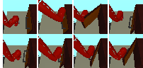
Figure 11: Examples of 8 skills learnt in Visual Door.

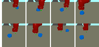
Figure 12: Examples of 8 skills learnt in Visual Pusher.

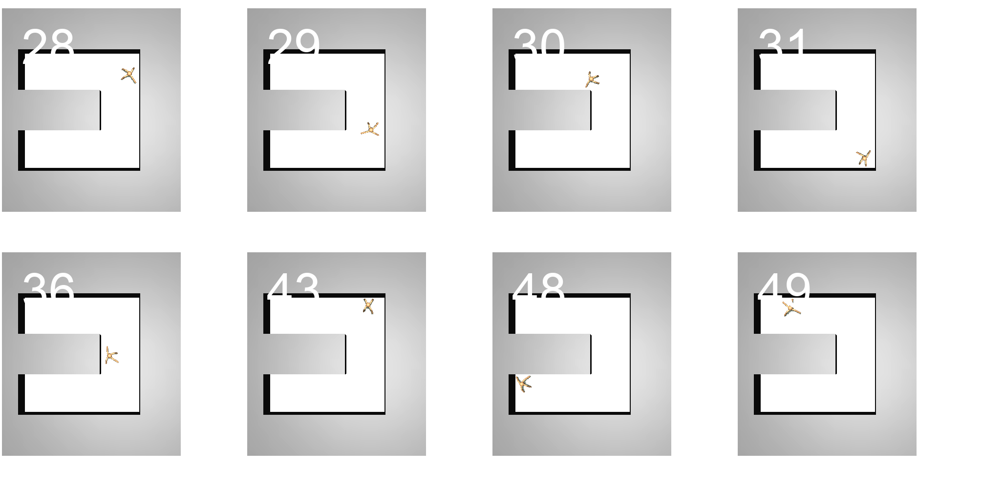
Figure 13: Examples of 8 skills learnt in Ant Maze.

References

- [1] Achiam, J., Edwards, H., Amodei, D., Abbeel, P.: Variational option discovery algorithms. CoRR abs/1807.10299 (2018)
- [2] Andrychowicz, M., Crow, D., Ray, A., Schneider, J., Fong, R., Welinder, P., McGrew, B., Tobin, J., Abbeel, P., Zaremba, W.: Hindsight experience replay. In: Annual Conference on Neural Information Processing Systems. pp. 5048–5058 (2017)
- [3] Aubret, A., Matignon, L., Hassas, S.: A survey on intrinsic motivation in reinforcement learning. arXiv preprint arXiv:1908.06976 (2019)
- [4] Aubret, A., Matignon, L., Hassas, S.: ELSIM: end-to-end learning of reusable skills through intrinsic motivation. In: Hutter, F., Kersting, K., Lijffijt, J., Valera, I. (eds.) Machine Learning and Knowledge Discovery in Databases - European Conference, ECML PKDD 2020, Proceedings, Part II. Lecture Notes in Computer Science, vol. 12458, pp. 541–556. Springer (2020)
- [5] Bacon, P.L., Harb, J., Precup, D.: The option-critic architecture. In: Proceedings of the AAAI Conference on Artificial Intelligence. vol. 31 (2017)
- [6] Bar, A., Talmon, R., Meir, R.: Option discovery in the absence of rewards with manifold analysis. In: International Conference on Machine Learning. pp. 664–674. PMLR (2020)
- [7] Bellemare, M.G., Srinivasan, S., Ostrovski, G., Schaul, T., Saxton, D., Munos, R.: Unifying count-based exploration and intrinsic motivation. In: Lee, D.D., Sugiyama, M., von Luxburg, U., Guyon, I., Garnett, R. (eds.) Advances in Neural Information Processing Systems 29: Annual Conference on Neural Information Processing Systems 2016, December 5-10, 2016, Barcelona, Spain. pp. 1471–1479 (2016)
- [8] Bengio, E., Thomas, V., Pineau, J., Precup, D., Bengio, Y.: Independently controllable features. CoRR abs/1703.07718 (2017)
- [9] Bengio, Y., Courville, A., Vincent, P.: Representation learning: A review and new perspectives. IEEE transactions on pattern analysis and machine intelligence 35(8), 1798–1828 (2013)
- [10] Bharadhwaj, H., Garg, A., Shkurti, F.: Leaf: Latent exploration along the frontier. arXiv e-prints pp. arXiv–2005 (2020)
- [11] Borsa, D., Barreto, A., Quan, J., Mankowitz, D.J., van Hasselt, H., Munos, R., Silver, D., Schaul, T.: Universal successor features approximators. In: 7th International Conference on Learning Representations, ICLR 2019, New Orleans, LA, USA, May 6-9, 2019. OpenReview.net (2019)
- [12] Burda, Y., Edwards, H., Pathak, D., Storkey, A.J., Darrell, T., Efros, A.A.: Large-scale study of curiosity-driven learning. In: 7th International Conference on Learning Representations, ICLR 2019, New Orleans, LA, USA, May 6-9, 2019. OpenReview.net (2019)
- [13] Campos, V., Trott, A., Xiong, C., Socher, R., Giro-i Nieto, X., Torres, J.: Explore, discover and learn: Unsupervised discovery of state-covering skills. In: International Conference on Machine Learning. pp. 1317–1327. PMLR (2020)
- [14] Chen, T., Kornblith, S., Norouzi, M., Hinton, G.: A simple framework for contrastive learning of visual representations. In: International conference on machine learning. pp. 1597–1607. PMLR (2020)
- [15] Chevalier-Boisvert, M., Willems, L.: Minimalistic gridworld environment for openai gym. https://github.com/maximecb/gym-minigrid (2018)
- [16] Chopra, S., Hadsell, R., LeCun, Y.: Learning a similarity metric discriminatively, with application to face verification. In: 2005 IEEE Computer Society Conference on Computer Vision and Pattern Recognition (CVPR’05). vol. 1, pp. 539–546. IEEE (2005)
- [17] Colas, C., Fournier, P., Sigaud, O., Oudeyer, P.: CURIOUS: intrinsically motivated multi-task, multi-goal reinforcement learning. CoRR abs/1810.06284 (2018)
- [18] Colas, C., Karch, T., Lair, N., Dussoux, J., Moulin-Frier, C., Dominey, P.F., Oudeyer, P.: Language as a cognitive tool to imagine goals in curiosity driven exploration. In: Larochelle, H., Ranzato, M., Hadsell, R., Balcan, M., Lin, H. (eds.) Advances in Neural Information Processing Systems 33: Annual Conference on Neural Information Processing Systems 2020, NeurIPS 2020, December 6-12, 2020, virtual (2020)
- [19] Ecoffet, A., Huizinga, J., Lehman, J., Stanley, K.O., Clune, J.: First return, then explore. Nature 590(7847), 580–586 (2021)
- [20] Eysenbach, B., Salakhutdinov, R., Levine, S.: Search on the replay buffer: Bridging planning and reinforcement learning. In: Wallach, H.M., Larochelle, H., Beygelzimer, A., d’Alché-Buc, F., Fox, E.B., Garnett, R. (eds.) Advances in Neural Information Processing Systems 32: Annual Conference on Neural Information Processing Systems 2019, NeurIPS 2019, December 8-14, 2019, Vancouver, BC, Canada. pp. 15220–15231 (2019)
- [21] Eysenbach, B., Gupta, A., Ibarz, J., Levine, S.: Diversity is all you need: Learning skills without a reward function. In: 7th International Conference on Learning Representations, ICLR 2019, New Orleans, LA, USA, May 6-9, 2019. OpenReview.net (2019)
- [22] Florensa, C., Duan, Y., Abbeel, P.: Stochastic neural networks for hierarchical reinforcement learning. In: 5th International Conference on Learning Representations, ICLR 2017, Toulon, France, April 24-26, 2017, Conference Track Proceedings. OpenReview.net (2017)
- [23] Florensa, C., Held, D., Geng, X., Abbeel, P.: Automatic goal generation for reinforcement learning agents. In: Dy, J.G., Krause, A. (eds.) Proceedings of the 35th International Conference on Machine Learning, ICML 2018, Stockholmsmässan, Stockholm, Sweden, July 10-15, 2018. Proceedings of Machine Learning Research, vol. 80, pp. 1514–1523. PMLR (2018)
- [24] Fournier, P., Colas, C., Chetouani, M., Sigaud, O.: Clic: Curriculum learning and imitation for object control in non-rewarding environments. IEEE Transactions on Cognitive and Developmental Systems (2019)
- [25] Fritzke, B., et al.: A growing neural gas network learns topologies. Advances in neural information processing systems 7, 625–632 (1995)
- [26] Ghosh, D., Gupta, A., Levine, S.: Learning actionable representations with goal conditioned policies. In: 7th International Conference on Learning Representations, ICLR 2019, New Orleans, LA, USA, May 6-9, 2019. OpenReview.net (2019), https://openreview.net/forum?id=Hye9lnCct7
- [27] Haarnoja, T., Zhou, A., Abbeel, P., Levine, S.: Soft actor-critic: Off-policy maximum entropy deep reinforcement learning with a stochastic actor. In: International Conference on Machine Learning. pp. 1861–1870. PMLR (2018)
- [28] Hansen, S., Dabney, W., Barreto, A., Warde-Farley, D., de Wiele, T.V., Mnih, V.: Fast task inference with variational intrinsic successor features. In: 8th International Conference on Learning Representations, ICLR 2020, Addis Ababa, Ethiopia, April 26-30, 2020. OpenReview.net (2020)
- [29] Hazan, E., Kakade, S., Singh, K., Van Soest, A.: Provably efficient maximum entropy exploration. In: International Conference on Machine Learning. pp. 2681–2691. PMLR (2019)
- [30] Jinnai, Y., Park, J.W., Machado, M.C., Konidaris, G.: Exploration in reinforcement learning with deep covering options. In: International Conference on Learning Representations (2019)
- [31] Kingma, D.P., Welling, M.: Auto-encoding variational bayes. In: Bengio, Y., LeCun, Y. (eds.) 2nd International Conference on Learning Representations, ICLR 2014, Banff, AB, Canada, April 14-16, 2014, Conference Track Proceedings (2014)
- [32] Kohonen, T.: The self-organizing map. Proceedings of the IEEE 78(9), 1464–1480 (1990)
- [33] Kovač, G., Laversanne-Finot, A., Oudeyer, P.Y.: Grimgep: learning progress for robust goal sampling in visual deep reinforcement learning. arXiv preprint arXiv:2008.04388 (2020)
- [34] Laversanne-Finot, A., Pere, A., Oudeyer, P.Y.: Curiosity driven exploration of learned disentangled goal spaces. In: Conference on Robot Learning. pp. 487–504. PMLR (2018)
- [35] Lee, L., Eysenbach, B., Parisotto, E., Xing, E.P., Levine, S., Salakhutdinov, R.: Efficient exploration via state marginal matching. CoRR abs/1906.05274 (2019)
- [36] Levy, A., Platt, R., Saenko, K.: Hierarchical reinforcement learning with hindsight. In: International Conference on Learning Representations (2019)
- [37] Li, S., Zheng, L., Wang, J., Zhang, C.: Learning subgoal representations with slow dynamics. In: International Conference on Learning Representations (2021), https://openreview.net/forum?id=wxRwhSdORKG
- [38] Lu, X., Tiomkin, S., Abbeel, P.: Predictive coding for boosting deep reinforcement learning with sparse rewards. CoRR abs/1912.13414 (2019)
- [39] Machado, M.C., Bellemare, M.G., Bowling, M.H.: A laplacian framework for option discovery in reinforcement learning. In: Precup, D., Teh, Y.W. (eds.) Proceedings of the 34th International Conference on Machine Learning, ICML 2017, Sydney, NSW, Australia, 6-11 August 2017. Proceedings of Machine Learning Research, vol. 70, pp. 2295–2304. PMLR (2017)
- [40] Marsland, S., Shapiro, J., Nehmzow, U.: A self-organising network that grows when required. Neural Networks 15(8-9), 1041–1058 (2002)
- [41] Metzen, J.H., Kirchner, F.: Incremental learning of skill collections based on intrinsic motivation. Frontiers in neurorobotics 7, 11 (2013)
- [42] Nachum, O., Gu, S., Lee, H., Levine, S.: Near-optimal representation learning for hierarchical reinforcement learning. arXiv preprint arXiv:1810.01257 (2018)
- [43] Nachum, O., Gu, S.S., Lee, H., Levine, S.: Data-efficient hierarchical reinforcement learning. In: Bengio, S., Wallach, H., Larochelle, H., Grauman, K., Cesa-Bianchi, N., Garnett, R. (eds.) Advances in Neural Information Processing Systems 31, pp. 3303–3313 (2018)
- [44] Nair, A., Pong, V., Dalal, M., Bahl, S., Lin, S., Levine, S.: Visual reinforcement learning with imagined goals. In: Bengio, S., Wallach, H.M., Larochelle, H., Grauman, K., Cesa-Bianchi, N., Garnett, R. (eds.) Advances in Neural Information Processing Systems 31: Annual Conference on Neural Information Processing Systems 2018, NeurIPS 2018, December 3-8, 2018, Montréal, Canada. pp. 9209–9220 (2018)
- [45] Nasiriany, S., Pong, V., Lin, S., Levine, S.: Planning with goal-conditioned policies. In: Wallach, H.M., Larochelle, H., Beygelzimer, A., d’Alché-Buc, F., Fox, E.B., Garnett, R. (eds.) Advances in Neural Information Processing Systems 32: Annual Conference on Neural Information Processing Systems 2019, NeurIPS 2019, December 8-14, 2019, Vancouver, BC, Canada. pp. 14814–14825 (2019)
- [46] van den Oord, A., Li, Y., Vinyals, O.: Representation learning with contrastive predictive coding. CoRR abs/1807.03748 (2018)
- [47] Oudeyer, P.Y., Kaplan, F.: What is intrinsic motivation? a typology of computational approaches. Frontiers in neurorobotics 1, 6 (2009)
- [48] Parisi, G.I., Kemker, R., Part, J.L., Kanan, C., Wermter, S.: Continual lifelong learning with neural networks: A review. Neural Networks 113, 54–71 (2019)
- [49] Pitis, S., Chan, H., Zhao, S., Stadie, B., Ba, J.: Maximum entropy gain exploration for long horizon multi-goal reinforcement learning. In: International Conference on Machine Learning. pp. 7750–7761. PMLR (2020)
- [50] Pong, V., Dalal, M., Lin, S., Nair, A., Bahl, S., Levine, S.: Skew-fit: State-covering self-supervised reinforcement learning. In: Proceedings of the 37th International Conference on Machine Learning, ICML 2020, 13-18 July 2020, Virtual Event. Proceedings of Machine Learning Research, vol. 119, pp. 7783–7792. PMLR (2020)
- [51] Riemer, M., Liu, M., Tesauro, G.: Learning abstract options. In: Bengio, S., Wallach, H.M., Larochelle, H., Grauman, K., Cesa-Bianchi, N., Garnett, R. (eds.) Advances in Neural Information Processing Systems 31: Annual Conference on Neural Information Processing Systems 2018, NeurIPS 2018, December 3-8, 2018, Montréal, Canada. pp. 10445–10455 (2018)
- [52] Savinov, N., Dosovitskiy, A., Koltun, V.: Semi-parametric topological memory for navigation. In: 6th International Conference on Learning Representations, ICLR 2018, Vancouver, BC, Canada, April 30 - May 3, 2018, Conference Track Proceedings. OpenReview.net (2018), https://openreview.net/forum?id=SygwwGbRW
- [53] Savinov, N., Raichuk, A., Vincent, D., Marinier, R., Pollefeys, M., Lillicrap, T.P., Gelly, S.: Episodic curiosity through reachability. In: 7th International Conference on Learning Representations, ICLR 2019, New Orleans, LA, USA, May 6-9, 2019. OpenReview.net (2019)
- [54] Schaul, T., Horgan, D., Gregor, K., Silver, D.: Universal value function approximators. In: International conference on machine learning. pp. 1312–1320. PMLR (2015)
- [55] Sharma, A., Gu, S., Levine, S., Kumar, V., Hausman, K.: Dynamics-aware unsupervised discovery of skills. In: 8th International Conference on Learning Representations, ICLR 2020, Addis Ababa, Ethiopia, April 26-30, 2020. OpenReview.net (2020)
- [56] Silver, D.L., Yang, Q., Li, L.: Lifelong machine learning systems: Beyond learning algorithms. In: Lifelong Machine Learning, Papers from the 2013 AAAI Spring Symposium, Palo Alto, California, USA, March 25-27, 2013. AAAI Technical Report, vol. SS-13-05. AAAI (2013)
- [57] Sutton, R.S., Barto, A.G.: Reinforcement learning: An introduction, vol. 1. MIT press Cambridge (1998)
- [58] Sutton, R.S., Precup, D., Singh, S.: Between mdps and semi-mdps: A framework for temporal abstraction in reinforcement learning. Artificial intelligence 112(1-2), 181–211 (1999)
- [59] Todorov, E., Erez, T., Tassa, Y.: Mujoco: A physics engine for model-based control. In: IEEE/RSJ IROS. pp. 5026–5033. IEEE (2012)
- [60] Warde-Farley, D., de Wiele, T.V., Kulkarni, T.D., Ionescu, C., Hansen, S., Mnih, V.: Unsupervised control through non-parametric discriminative rewards. In: 7th International Conference on Learning Representations, ICLR 2019, New Orleans, LA, USA, May 6-9, 2019. OpenReview.net (2019)
- [61] Wiskott, L., Sejnowski, T.J.: Slow feature analysis: Unsupervised learning of invariances. Neural computation 14(4), 715–770 (2002)
- [62] Zhang, Y., Abbeel, P., Pinto, L.: Automatic curriculum learning through value disagreement. Advances in Neural Information Processing Systems 33 (2020)
- [63] Zhao, R., Sun, X., Tresp, V.: Maximum entropy-regularized multi-goal reinforcement learning. In: International Conference on Machine Learning. pp. 7553–7562. PMLR (2019)
- [64] Zhou, X., Bai, T., Gao, Y., Han, Y.: Vision-based robot navigation through combining unsupervised learning and hierarchical reinforcement learning. Sensors 19(7), 1576 (2019)