Abstract

Monge map refers to the optimal transport map between two probability distributions and provides a principled approach to transform one distribution to another. Neural network based optimal transport map solver has gained great attention in recent years. Along this line, we present a scalable algorithm for computing the neural Monge map between two probability distributions. Our algorithm is based on a weak form of the optimal transport problem, thus it only requires samples from the marginals instead of their analytic expressions, and can accommodate optimal transport between two distributions with different dimensions. Our algorithm is suitable for general cost functions, compared with other existing methods for estimating Monge maps using samples, which are usually for quadratic costs. The performance of our algorithms is demonstrated through a series of experiments with both synthetic and realistic data, including text-to-image generation and image inpainting tasks.

1 Introduction

The past decade has witnessed great success of optimal transport (OT) (Villani,, 2008) based applications in machine learning community (Arjovsky et al.,, 2017; Krishnan and Martínez,, 2018; Li et al.,, 2019; Makkuva et al.,, 2020; Inoue et al.,, 2020; Ma et al.,, 2020; Fan et al.,, 2020; Haasler et al.,, 2020; Alvarez-Melis and Fusi,, 2020; Alvarez-Melis et al.,, 2021; Bunne et al.,, 2021; Mokrov et al.,, 2021; Bunne et al.,, 2022; Yang and Uhler,, 2018; Fan et al., 2022a, ). The Wasserstein distance induced by OT is widely used to evaluate the discrepancy between distributions thanks to its weak continuity and robustness. In this work, given any two probability distributions $\rho_{a}$ and $\rho_{b}$ defined on $\mathbb{R}^{n}$ and $\mathbb{R}^{m}$, we consider the Monge problem

$$C_{\textrm{Monge}}(\rho_{a},\rho_{b})\triangleq\min_{\begin{subarray}{c}T:\mathbb{R}^{n}\rightarrow\mathbb{R}^{m},\\ T_{\sharp}\rho_{a}=\rho_{b}\end{subarray}}\int_{\mathbb{R}^{n}}c(x,T(x))\rho_{a}(x)~{}dx.$$ (1)

Here $c(x,y)$ denotes the cost of transporting from $x$ to $y$ and $T$ is the transport map. We define the pushforward of distribution $\rho_{a}$ by $T$ as $T_{\sharp}\rho_{a}(E)=\rho_{a}(T^{-1}(E))$ for any measurable set $E\subset\mathbb{R}^{m}$. The Monge problem seeks the cost-minimizing transport plan $T_{*}$ from $\rho_{a}$ to $\rho_{b}$. The optimal $T_{*}$ is also known as the Monge map of (1).

Solving (1) in high dimensional space yields a challenging problem due to the curse of dimensionality for discretization. A modern formulation of Monge problem as a linear programming problem known as Kantorovich problem (Villani,, 2003), and adding an entropic regularization, one is capable of computing the problem via iterative Sinkhorn algorithm (Cuturi,, 2013). Such type of treatment has been widely accepted since it is friendly to high dimensional cases (Altschuler et al.,, 2017; Genevay et al.,, 2018; Li et al.,, 2019; Xie et al.,, 2020), but the algorithm does not scale well to a large number of samples and is not suitable to handle continuous probability measures. Moreover, the transport map/plan obtained with this strategy cannot be generalized to unseen samples.

In this work, we propose a scalable algorithm for estimating the Wasserstein distance as well as the optimal map in continuous spaces without introducing any regularization terms. Particularly, we apply the Lagrangian multiplier directly to Monge problem, and obtain a minimax problem. Our contribution is summarized as follows: 1) We develop a neural network based algorithm to compute the optimal transport map associated with general transport costs between any two distributions given their unpaired samples; 2) Our method is capable of computing OT problems between distributions over spaces that do not share the same dimension. 3) We provide a rigorous error analysis of the algorithm based on duality gaps; 4) We demonstrate its performance and its scaling properties in truly high dimensional setting through various experiments.

As other computational OT methods, our method does not require paired data for learning the transport map. In real world, the acquirement and maintenance of large-scale paired data are laborious. We will show that our proposed algorithm can be applied to multiple cutting-edge tasks, where the dominant methods still require paired data. In particular, our examples include text-to-image generation and image inpainting, which would confirm that our algorithm can achieve competitive results even without paired data.

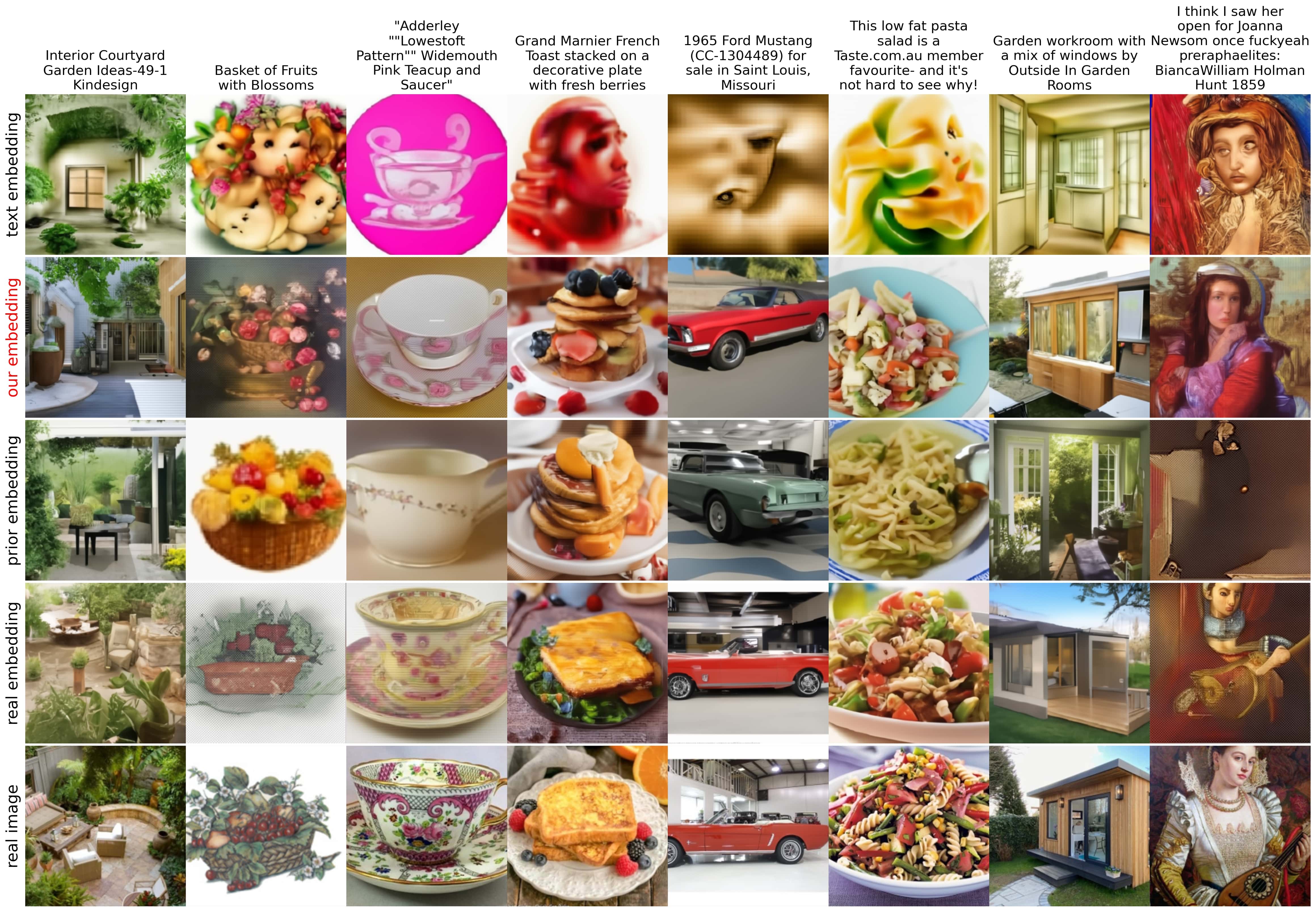
Figure 1: Random image samples with size $224\times 224$ on Laion art testing prompts. Except for the last row of real images, we show the outputs of the same decoder with different conditions. The condition of decoder includes a text encoding, which we keep unchanged across rows, and an image embedding. In the first row, we feed the decoder the text embedding, and the generated images are unrealistic because the image and the text embeddings are not interchangeable. In the second row, we pass the embedding pushforwarded by our transport map, which is trained on unpaired data. As a baseline method, we pass an image embedding generated by the diffusion prior in DALL$\cdot$E2-Laion, which is trained on paired data. To explicitly show the decoder’s recovery ability, we pass the real image embedding in the fourth row.

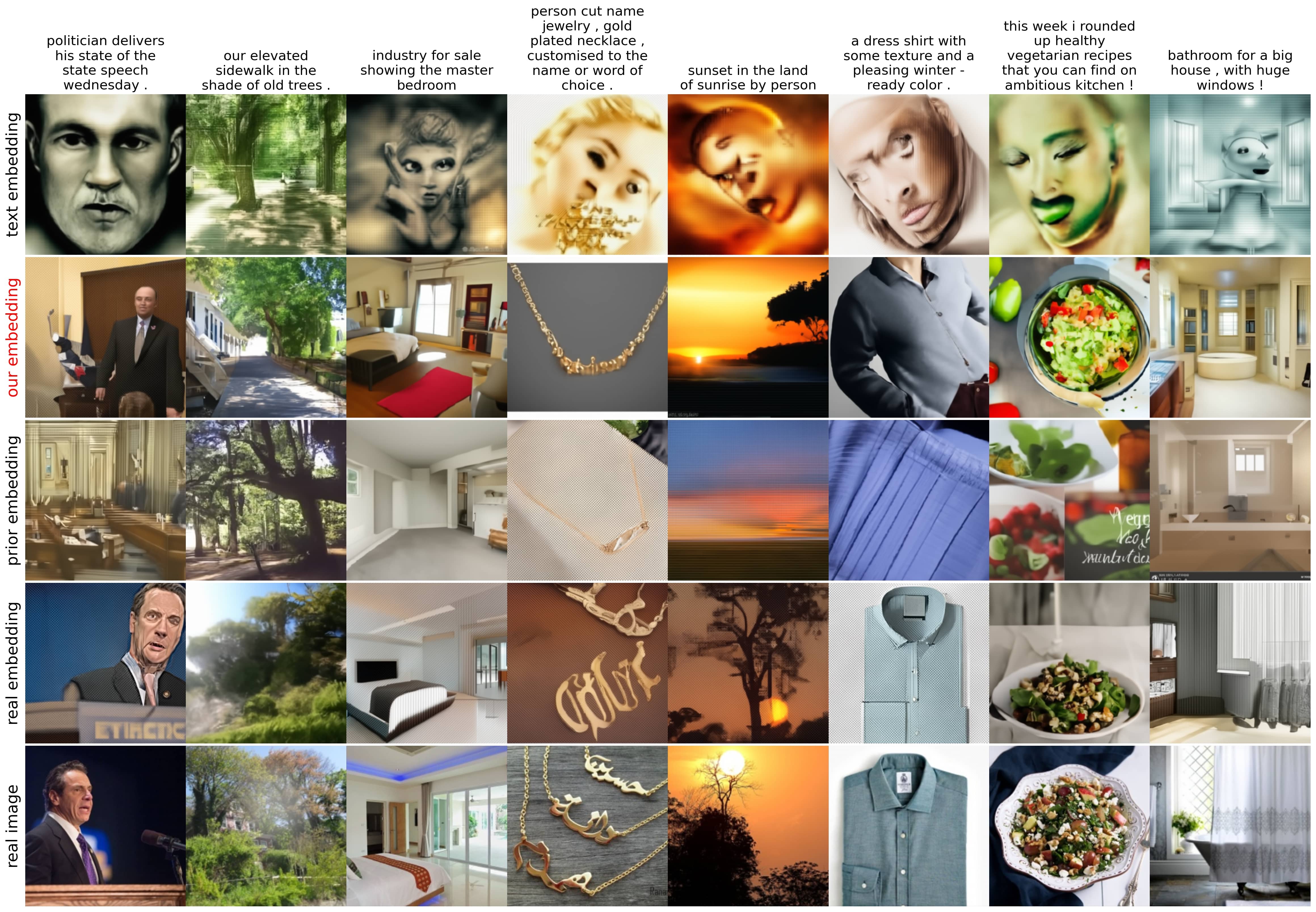
Figure 2: Random image samples on Conceptual Captions 3M prompts. The meaning of each row is the same as in Figure 1.

2 A brief background of OT problems

The general OT problem from $\mathbb{R}^{n}$ to $\mathbb{R}^{m}$ is formulated as

$$C(\rho_{a},\rho_{b}):=\inf_{\pi\in\Pi(\rho_{a},\rho_{b})}\int_{\mathbb{R}^{n}\times\mathbb{R}^{m}}c(x,y)d\pi(x,y),$$ (2)

where we define $\Pi(\rho_{a},\rho_{b})$ as the set of joint distributions on $\mathbb{R}^{n\times m}$ with marginals equal to $\rho_{a}$ and $\rho_{b}$. In this work, we will mainly focus on the cost function $c(\cdot,\cdot)$ that is well-defined and regular. The detailed assumptions of our considered cost functions are presented in (9), (10) and (11) in Appendix A.

The Kantorovich dual formulation of the primal OT problem (2) is (Chap 5, Villani, (2008))

$$\sup_{\phi,\psi}\left\{\int_{\mathbb{R}^{m}}\phi(y)\rho_{b}(y)~{}dy-\int_{\mathbb{R}^{n}}\psi(x)\rho_{a}(x)~{}dx\right\},$$ (3)

where the maximization is over all $\psi\in L^{1}(\rho_{a})$, $\phi\in L^{1}(\rho_{b})$ that satisfy $\phi(y)-\psi(x)\leq c(x,y)$ for any $x\in\mathbb{R}^{n},y\in\mathbb{R}^{m}$.

For further discussions on the dual problem (3), as well as the equivalence between the primal OT problem (2) and its Kantorovich dual (3), we refer the reader to Appendix A.

In general, the optimal solution $\pi_{*}$ of (2) can be treated as a random transport plan, i.e., we are allowed to break a single particle into pieces and then transport each piece to certain positions according to the plan $\pi_{*}$. However, in this study, we will mainly focus on computing for the deterministic optimal map $T_{*}$ of the classical version of the OT problem, which is the Monge problem.

The following theorem states the existence and uniqueness of the optimal solution to the Monge problem. It also reveals the relation between the optimal map $T_{*}$ and the optimal transport plan $\pi_{*}$. A more complete statement of this theorem can be found in Appendix A.

Theorem 1.

(Informal) Suppose the cost $c$ satisfies (9), (10), (11), and assume that $\rho_{a}$ and $\rho_{b}$ are compactly supported and $\rho_{a}$ is absolute continuous with respect to the Lebesgue measure on $\mathbb{R}^{n}$. Then there exists a unique-in-law transport map $T_{*}$ solving Monge problem (1). Furthermore, $(\textrm{Id},T_{*})_{\sharp}\rho_{a}$ is an optimal solution to the OT problem (2).

3 Proposed method

In order to formulate a tractable algorithm for the general Monge problem (1), we first notice that (1) is a constrained optimization problem. Thus, we introduce a Lagrange multiplier $f$ for the constraint $T_{\sharp}\rho_{a}=\rho_{b}$ and reformulate (1) as a saddle point problem

$$\sup_{f}\inf_{T}\mathcal{L}(T,f),$$ (4)

where $\mathcal{L}(T,f)$ equals

$$\int_{\mathbb{R}^{n}}c(x,T(x))\rho_{a}dx+\int_{\mathbb{R}^{m}}f(y)(\rho_{b}-T_{\sharp}\rho_{a})dy$$

$$= \int_{\mathbb{R}^{n}}\!\!\!\left[c(x,T(x))-f(T(x))\right]\rho_{a}dx+\int_{\mathbb{R}^{m}}\!\!f(y)\rho_{b}dy.$$ (5)

The following theorem ensures the consistency of the max-min formulation (4). The proof is provided in Section C

Theorem 2 (Consistency).

Suppose the max-min problem (4) admits at least one saddle point solution. We denote it as $(\bar{T},\bar{f})$. Under the assumption $\bar{T}_{\sharp}\rho_{a}=\rho_{b}$, we have

• $\phi=\bar{f}$ is an optimal solution to the Kantorovich dual problem (3).

• The optimal solution to the Monge problem (1) exists, and $\bar{T}$ is an optimal solution.

• $\mathcal{L}(\bar{T},\bar{f})=C_{\textrm{Monge}}(\rho_{a},\rho_{b})$.

Without the assumption $\bar{T}_{\sharp}\rho_{a}=\rho_{b}$, we no longer have the guarantee on the existence of Monge map $T_{*}$, not to mention the consistency between $\bar{T}$ and $T_{*}$. However, we are still able to show the consistency between the saddle point value $\mathcal{L}(\bar{T},\bar{f})$ and the general OT distance $C(\rho_{a},\rho_{b})$.

Theorem 3 (Consistency without $\bar{T}_{\sharp}\rho_{a}=\rho_{b}$).

Suppose the max-min problem (4) admits at least one saddle point solution $(\bar{T},\bar{f})$, then $\mathcal{L}(\bar{T},\bar{f})=C(\rho_{a},\rho_{b})$.

The proof to Theorem 3 and the related example are presented in Appendix C. In implementation, we parametrize both the map $T$ and the dual variable $f$ by the neural networks $T_{\theta},f_{\eta}$, with $\theta,\eta$ being the parameters of the networks. Consequently, our goal becomes solving the following saddle point problem

$$\max_{\eta}\min_{\theta} ~{}\mathcal{L}(T_{\theta},f_{\eta}):=$$ (6)

$$\frac{1}{N}\sum_{k=1}^{N}c({X_{k}},T_{\theta}({X_{k}}))-f_{\eta}(T_{\theta}({X_{k}}))+f_{\eta}({Y_{k}})$$

where $N$ is size of the datasets and $\{X_{k}\},\{Y_{k}\}$ are samples drawn by $\rho_{a}$ and $\rho_{b}$ separately. The algorithm is summarized in Algorithm 1. The computational complexity of our algorithm is similar with Generative Adversarial Network (GAN)-type methods. In particular, Algorithm 1 requires $\mathcal{O}(K(K_{1}+K2)B)$ operations in total.

Algorithm 1 Computing optimal Monge map from $\rho_{a}$ to $\rho_{b}$

1:Input: Marginal distributions $\rho_{a}$ and $\rho_{b}$, Batch size $B$, Cost function $c(x,y)$.

2:Initialize ${T}_{\theta},{f}_{\eta}$.

3:for $K$ steps do

4:     Sample $\{X_{k}\}_{k=1}^{B}$ $\sim\rho_{a}$. Sample $\{Y_{k}\}_{k=1}^{B}$ $\sim\rho_{b}$.

5:     Update ${\theta}$ to decrease (6) for $K_{1}$ steps.

6:     Update ${\eta}$ to increase (6) for $K_{2}$ steps.

7:end for

8:Output: The transport map $T_{\theta}$.

Comparison with GAN

It is worth pointing out that our method and the Wasserstein Generative Adversarial Network (WGAN) Arjovsky et al., (2017) are similar in the sense that they are both carrying out minimization over the generator/transport map and maximization over the discriminator/dual potential. However, there are two main distinctions, which are summarized in the following.

• (Purpose: arbitrary map vs optimal map) The purpose of WGAN is to compute for an arbitrary map $T$ such that $T_{\sharp}\rho_{a}$ is close to the target distribution $\rho_{b}$; On the other hand, the purpose of our method is two-folds: we not only compute for the map $T$ that pushforwards $\rho_{a}$ to $\rho_{b}$, but also guarantee the optimality of $T$ in the sense of minimizing the total transportation cost $\mathbb{E}_{X\sim\rho_{a}}c(X,T(X))$.

• (Designing logic: minimizing distance vs computing distance itself) In WGAN, one aims at minimizing the OT distance as the discrepancy between $T_{\sharp}\rho_{a}$ and the target distribution $\rho_{b}$, the optimal value of the corresponding loss function thus equals to 0; In contrast, our proposed method computes OT distance (as well as the transport map) between source distribution $\rho_{a}$ and the target $\rho_{b}$. In this case, the optimal value of the associated loss function equals $C_{\textrm{Monge}}(\rho_{a},\rho_{b})$.

We provide more detailed discussion on the comparison between our method and WGAN in Appendix B.

4 Error Estimation via Duality Gaps

In this section, we assume $m=n=d$, i.e. we consider Monge problem on $\mathbb{R}^{d}$. Suppose we solve (4) to a certain stage and obtain the pair $(T,f)$, inspired by Hütter and Rigollet, (2020) and Makkuva et al., (2020), we provide an a posterior estimate to a weighted $L^{2}$ error between our computed map $T$ and the optimal Monge map $T_{*}$. Before we present our result, we need the following assumptions

Assumption 1 (on cost $c(\cdot,\cdot)$).

We assume $c\in C^{2}(\mathbb{R}^{d}\times\mathbb{R}^{d})$ is bounded from below. Furthermore, for any $x,y\in\mathbb{R}^{d}$, we assume $\partial_{x}c(x,y)$ is injective w.r.t. $y$; $\partial_{xy}c(x,y)$, as a $d\times d$ matrix, is invertible; and $\partial_{yy}c(x,y)$ is independent of $x$.

Assumption 2 (on marginals $\rho_{a}$, $\rho_{b}$).

We assume that $\rho_{a},\rho_{b}$ are compactly supported on $\mathbb{R}^{d}$, and $\rho_{a}$ is absolutely continuous w.r.t. the Lebesgue measure.

Assumption 3 (on dual variable $f$).

Assume the dual variable $f\in C^{2}(\mathbb{R}^{d})$ is always taken from $c$-concave functions, i.e., there exists certain $\varphi\in C^{2}(\mathbb{R}^{d})$ such that $f(\cdot)=\inf_{x}\{\varphi(x)+c(x,\cdot)\}$ (c.f. Definition 5.7 of Villani, (2008)). Furthermore, we assume that there exists a unique minimizer $x_{y}\in\textrm{argmin}_{x}\{\varphi(x)+c(x,y)\}$ for any $y\in\mathbb{R}^{d}$. And the Hessian of $\varphi(\cdot)+c(\cdot,y)$ at $x_{y}$ is positive definite.

For the sake of conciseness, let us introduce two notations. We denote $\sigma(x,y)=\sigma_{\min}(\partial_{xy}c(x,y))>0$ as the minimum singular value of $\partial_{xy}c(x,y)$; and denote $\lambda(y)=\lambda_{\max}(\nabla^{2}_{xx}(\varphi(x)+c(x,y))|_{x=x_{y}})>0$ as the maximum eigenvalue of the Hessian of $\varphi(\cdot)+c(\cdot,y)$ at $x_{y}$.

We denote the duality gaps as

$$\mathcal{E}_{1}(T,f)=\mathcal{L}(T,f)-\inf_{\widetilde{T}}\mathcal{L}(\widetilde{T},f),$$

$$\mathcal{E}_{2}(f)=\sup_{\widetilde{f}}\inf_{\widetilde{T}}\mathcal{L}(\widetilde{T},\widetilde{f})-\inf_{\widetilde{T}}\mathcal{L}(\widetilde{T},f).$$

It is not hard to verify that the conditions mentioned in Theorem 1 are satisfied under Assumption 1 and Assumption 2. Thus the Monge map $T_{*}$ to the Monge problem (1) exists and is unique. We now state the main theorem on error estimation:

Theorem 4 (Posterior Error Enstimation via Duality Gaps).

Suppose Assumption 1, 2 and 3 hold. Let us further assume the max-min problem (4) admits a saddle point $(\bar{f},\bar{T})$ that is consistent with the Monge problem, i.e. $\bar{T}$ equals $T_{*}$, $\rho_{a}$ almost surely. Then there exists a strict positive weight function $\beta(x)>\underset{y\in\mathbb{R}^{m}}{\min}\left\{\frac{\sigma(x,y)}{2\lambda(y)}\right\}$ such that the weighted $L^{2}$ error between computed map $T$ and the Monge map $T_{*}$ is upper bounded by

$$\|T-T_{*}\|_{L^{2}(\beta\rho_{a})}\leq\sqrt{2(\mathcal{E}_{1}(T,f)+\mathcal{E}_{2}(f))}.$$

The exact formulation of $\beta$ is provided in (32) in the appendix D.

Sketch of proof .

Let us denote $\Psi_{x}(y)=f(y)-c(x,y)$. A key step of the proof is to show certain concavity of $\Psi_{x}(\cdot)$ given $f$ as a $c-$concave function (c.f. Assumption 3). This is proved in Lemma 3 in Appendix D.

Once $\Psi_{x}(\cdot)$ is concave, there exists unique $T_{f}(x)\in\textrm{argmax}_{y}\{\Psi_{x}(y)\}$. Thus we are able to write $\mathcal{E}_{1}(f,T)$ as

$$\mathcal{E}_{1}(T,f)= -\int[f(T(x))-c(x,T(x))]\rho_{a}~{}dx$$

$$+\sup_{\widetilde{T}}\left\{\int[f(\widetilde{T}(x))-c(x,\widetilde{T}(x))]\rho_{a}~{}dx\right\}$$

$$= \int[\Psi_{x}(T_{f}(x))-\Psi_{x}(T(x))]\rho_{a}(x)~{}dx.$$

The concavity of $\Psi_{x}$ then leads to

$$\mathcal{E}_{1}(T,f)\geq\|T_{f}-T\|_{L^{2}(\beta\rho_{a})}^{2},$$ (7)

where $\beta(\cdot)$ depends on the concavity of $\Psi_{x}(\cdot)$.

Similarly, we can rewrite $\mathcal{E}_{2}(f)$ as

$$\mathcal{E}_{2}(f)=\int[\Psi_{x}(T_{f}(x))-\Psi_{x}(\bar{T}(x))]\rho_{a}(x)~{}dx.$$

By the similar concavity argument, one can prove $\mathcal{E}_{2}(T,f)\geq\|T_{f}-\bar{T}\|_{L^{2}(\beta\rho_{a})}^{2}$. Furthermore, since $\bar{T}=T_{*}$, $\rho_{a}$ almost surely, we have the following estimation

$$\mathcal{E}_{2}(T,f)\geq\|T_{f}-T_{*}\|_{L^{2}(\beta\rho_{a})}^{2}.$$ (8)

Finally, applying the triangle inequality to (7), (8) leads to the desired estimation. ∎

Remark 1.

We can verify that $c(x,y)=\frac{1}{2}\|x-y\|^{2}$ or $c(x,y)=-x\cdot y$ satisfy the conditions mentioned above. More specifically, when $c(x,y)=-x\cdot y$, then $\sigma(x,y)=1$, and $\lambda(y)=\frac{1}{\lambda_{\min}(\nabla^{2}f(y))}$. This recovers the upper bounds of Theorem 3.6 mentioned in Makkuva et al., (2020).

Remark 2.

Suppose $c$ satisfies Assumption 1. If $c$ is also an analytical function, then $c$ has the particular form $\Psi(x)+F(x)^{\top}y+\Phi(y)$, where $\Psi,u,\Phi$ are analytical functions on $\mathbb{R}^{d}$, and $F:\mathbb{R}^{d}\rightarrow\mathbb{R}^{d}$ is analytic with invertible Jacobian $DF(x)$ at any $x\in\mathbb{R}^{d}$.

5 Related work

Discrete OT methods (Courty et al.,, 2016; Feydy et al.,, 2020; Pooladian and Niles-Weed,, 2021; Meng et al.,, 2019) solve the Kantorovich formulation with EMD (Nash,, 2000) or Sinkhorn algorithm (Cuturi,, 2013). It normally computes an optimal coupling of two empirical distributions, and cannot provide out-of-sample estimates. With an additional parameterization of a mapping function, such as linear or kernel function space (Perrot et al.,, 2016), they can map the unseen data. However, this map is not the solution of Monge problem but only an approximation of the optimal coupling (Courty et al.,, 2017, Sec. 2.1). Perrot et al., (2016) requires solving the matrix inverse when updating the transformation map, thus introduces a risk of instability. Their function space of the map is also less expressive as neural networks, which makes it difficult to solve the OT problem with complex transport costs and high dimension data. Moreover, they can not handle large scale datasets.

With the rise of neural networks, neural OT has become popular with an advantage of dealing with continuous measure. Seguy et al., (2017); Genevay et al., (2016) solve the regularized OT problem, and as such introduce the bias. Another branch of work (Makkuva et al.,, 2020; Korotin et al., 2021a, ; Fan et al.,, 2020; Korotin et al., 2021c, ) comes with parameterizing Brenier potential by Input Convex Neural Network (ICNN) (Amos et al.,, 2017). The notable work (Makkuva et al.,, 2020) is special case of our formula. In particular, their dual formula reads

$$\sup_{h}\inf_{g}-\int[{\langle}x,\nabla g(x)-h(\nabla g(x)){\rangle}]\rho_{a}dx-\int h(y)\rho_{b}dy,$$

where $g,h$ are ICNN. After a change of variable $\nabla g=T,h=-f+\|\cdot\|^{2}/2$, it becomes the same as our (5) equipped with the cost $c(x,y)=\|x-y\|^{2}/2$. Later, the ICNN parameterization was shown to be less suitable (Korotin et al., 2021b, ; Fan et al., 2022b, ; Korotin et al., 2022a, ) for large scale problems because ICNN is not expressive enough.

Recently, several works have illustrated the scalability of our dual formula with different realizations of the transportation costs. When $c(x,y)=\|x-y\|_{2}^{2}/2$, our method directly boils down to reversed maximum solver (Nhan Dam et al.,, 2019), which appears to be the best neural OT solvers among multiple baselines (Korotin et al., 2021b, ). Another variant (Rout et al.,, 2022) of our work obtains comparable performance in image generative models, which asserts the efficacy in unequal dimension tasks. Gazdieva et al., (2022) utilizes the same dual formula with more diverse costs in image super-resolution task.

Based on the similar dual formula, several works propose to add random noise as an additional input to make the map stochastic, i.e. one-to-many mapping, so it can approximate the Kantorovich OT plan. To make the learning of stochastic map valid, Korotin et al., 2022b extends the transport cost $c(x,y)$ to be weak cost that depends on the mapped distribution. Typically, they involve the variance in the weak cost to enforce the diversity. The stochastic map is, however, not suitable for our problem (1) because of the conditional collapse behavior (Korotin et al., 2022b, , Sec 5.1). Later, Asadulaev et al., (2022) extends the dual formula to more general cost functional. We note that the term general cost in Asadulaev et al., (2022) is different with general cost in our paper. Their formula is general in a higher level and extends ours.

6 Experiments

In this section, we specialize (5) with different general costs $c(x,y)$ to fit in various applications. We will not focus on the quadratic cost $c(x,y)=\|x-y\|_{2}^{2}$ since our formula in this special case has been extensively studied in multiple scenarios, e.g. generative model (Rout et al.,, 2022), super-resolution (Gazdieva et al.,, 2022), and style transfer (Korotin et al., 2022b, ). Instead, we focus on data with specific structure, which will be revealed in the cost function.

6.1 Unpaired text to image generation

We consider the task of generating images given text prompts. Existing successful text to image generation algorithms (Ramesh et al.,, 2021, 2022; Saharia et al.,, 2022) are supervised learning methods, and as such rely on paired data. In real world, it can be exhausting to maintain large-scale paired datasets given that they are mostly web crawling data, and the validity period of web data is limited. We intend to learn a map between the the text and image embedding space of the CLIP model without paired data. Our framework is shown in Figure 3. We use the same unpaired data generation scheme as Rout et al., (2022).

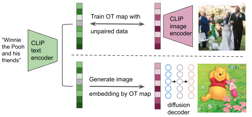
Figure 3: Our pipeline is motivated by DALL$\cdot$E2 (Ramesh et al.,, 2022). During the training (above the dotted line), our map learns to generate image embeddings that maximize the expected similarity with text embeddings. During the evaluation (below dotted line), given a text encoding (omitted from the figure) and a text embedding from the CLIP model, our map outputs an image embedding, which conditions a pretrained diffusion decoder to generate an image. The CLIP encoder and diffusion decoder are both pretrained and frozen.

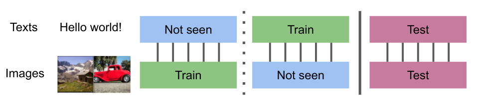
Figure 4: Our unpaired data generation process: we split a paired text-image dataset training into two parts: $\mathcal{S}$ and $\mathcal{T}$, and take the texts from $\mathcal{S}$ and images from $\mathcal{T}$ as our training data. Finally, we use the paired test data so we can compare with the real images.

In our algorithm, the sample from source distribution $\rho_{a}$ is composed of a text encoding $Q\in{\mathbb{R}}^{77\times 768}$ and a text embedding $x\in{\mathbb{R}}^{768}$ from CLIP (Radford et al.,, 2021) model, and the sample from target distribution $\rho_{b}$ is the image embedding $y\in{\mathbb{R}}^{768}$. The CLIP model is pretrained on 400M (text, image) pairs of web data with contrastive loss, such that the paired text and image embeddings share a large cosine similarity, and the non-paired embeddings present a small similarity. As a result, we choose the transport cost as the negative cosine similarity

$$c(x,y)=-\text{cos-sim}(x,y)=-\frac{{\langle}x,y{\rangle}}{\|x\|_{2}\|y\|_{2}},$$

which would enforce our map to generate an image embedding relevant to the input text.

We evaluate our algorithm on two datasets: Laion art and Conceptual captions 3M (CC-3M). Laion art dataset is filtered from a 5 billion dataset to have the high aesthetic level, which is suitable for the learning of image generation, while CC-3M is not curated. We use the OpenAI’s CLIP (ViT-L/14) model and a DALL$\cdot$E2 diffusion decoder. The training of their diffusion decoder requires paired data and its train dataset includes Laion art but not CC-3M. Therefore, our results on CC-3M are fully based on the unpaired data because no part in Figure 3 has seen paired data of CC-3M, while on Laion art, the diffusion decoder has some paired data information gained from pretraining.

We show qualitative samples in Figure 1 and 2, where we compare with DALL$\cdot$E2-Laion, a DALL$\cdot$E2 model pretrained on the paired Laion aesthetic dataset, which includes Laion art dataset. Figure 1 confirms that our transport map can generate image embeddings with comparable quality even without paired data. Since CC-3M is a zero-shot dataset for DALL$\cdot$E2-Laion, the performance of DALL$\cdot$E2-Laion clearly drops in Figure 2, while our model still generates reasonable images.

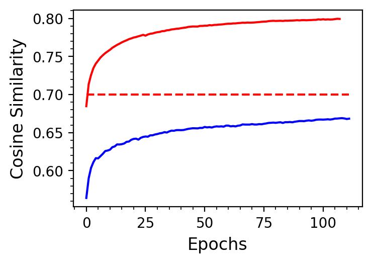
(a)

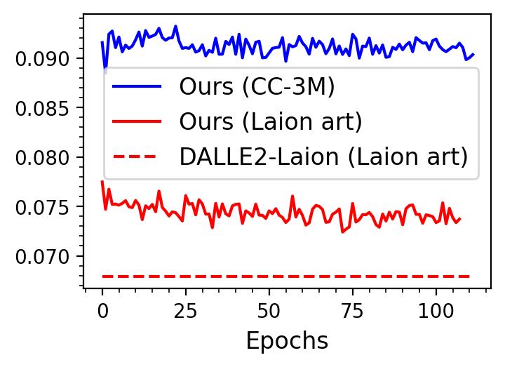
(b)

Figure 5: Averaged cosine similarity between the generated image embeddings and a) the ground truth image embeddings b) the unrelated text embeddings. The similarity in the left depicts how well the model recovers the real image embedding, and the similarity in the right quantifies the overfitting behaviour (the lower the better).

We also quantitatively compare with the baseline in terms of cosine similarity in Figure 5. Our method achieves higher cosine similarity w.r.t. the real images on Laion art dataset. In practice, we observe that the relevance of each (text, image) pair in CC-3M is more noisy than Laion art, which makes the model more difficult to learn the real image embedding. This expalins why our cosine similarity w.r.t real image embedding on CC-3M can not converge to the same level as Laion art. In the mean time, our overfitting level is very low on both datasets.

6.2 Image inpainting

In this section, we show the effectiveness of our method on the inpainting task with random rectangle masks. We take the distribution of occluded images to be $\rho_{a}$ and the distribution of the full images to be $\rho_{b}$. In many inpainting works, it’s assumed that an unlimited amount of paired training data is accessible (Zeng et al.,, 2021). However, most real-world applications do not involve the paired datasets. Accordingly, we consider the unpaired inpainting task, i.e. no pair of masked image and original image is accessible. The training and test data are generated in the same way as Figure 4. We choose cost function to be mean squared error (MSE) in the unmasked area

$$c(x,y)=\alpha\cdot\frac{\|x\odot M-y\odot M\|_{2}^{2}}{n},$$

where $M$ is a binary mask with the same size as the image. $M$ takes the value 1 in the unoccluded region, and 0 in the unknown/missing region. $\odot$ represents the point-wise multiplication, $\alpha$ is a tunable coefficient, and $n$ is dimension of $x$. Intuitively, this works as a regularization that the pushforward images should be consistent with input images in the unmasked area. Empirically, the map learnt with a larger $\alpha$ can generate more realistic images with natural transition in the mask border and exhibit more details on the face (c.f. Figure 14 in the appendix).

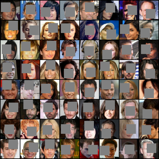
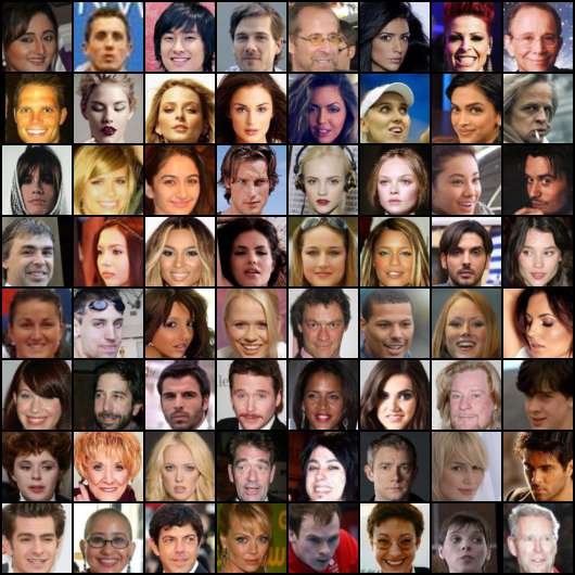
(a) Masked and real images

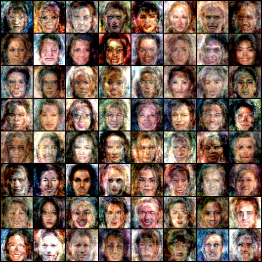
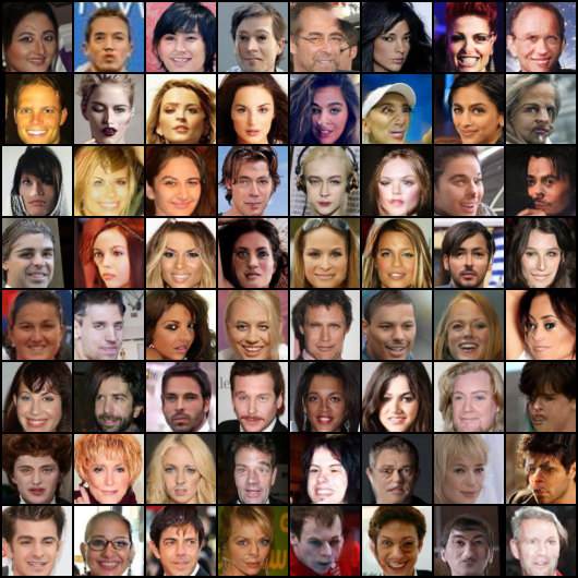
(b) Pushforward images $T(x)$

Figure 6: Unpaired image inpainting on test dataset of CelebA $64\times 64$. In panel (b), we show the pushforward images of the discrete OT method (Perrot et al.,, 2016) in the first row and ours in the second row.

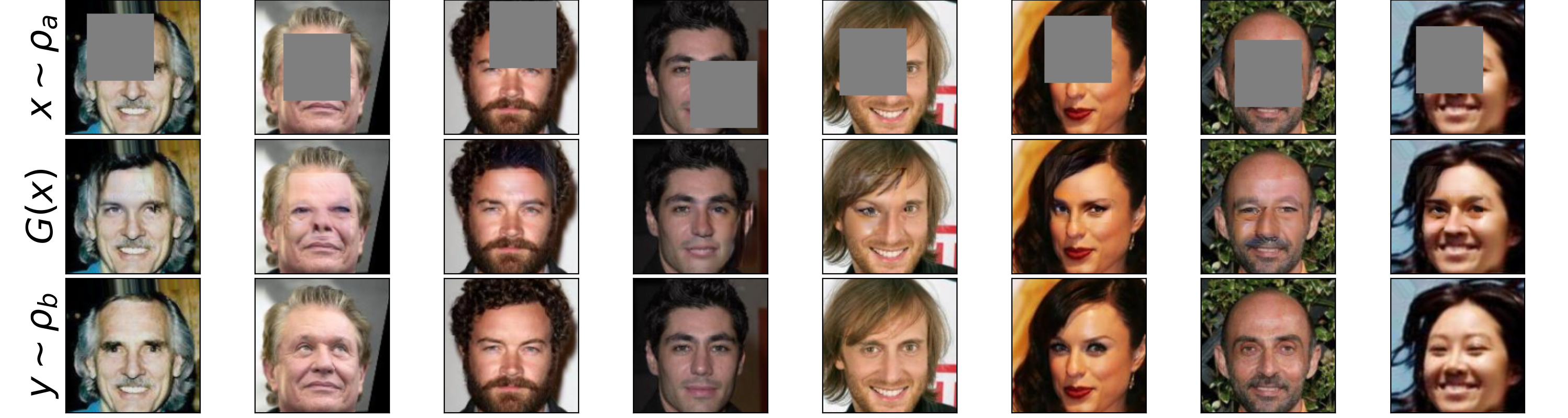
Figure 7: Unpaired image inpainting on test dataset of CelebA $128\times 128$. Denote $M^{C}$ as the complement of $M$, i.e. $M^{C}=1$ in the occluded area and $0$ otherwise. We take the composite image $G(x)=T(x)\odot M^{C}+x\odot M$ as the output image.

We conduct the experiments on CelebA $64\times 64$ and $128\times 128$ datasets (Liu et al.,, 2015). The input images ($\rho_{a}$) are occluded by randomly positioned square masks. Each of the source $\rho_{a}$ and target $\rho_{b}$ distributions contains $80k$ images. We present the empirical results of inpainting in Figure 6 and 7. In Figure 6, we compare with the discrete OT method Perrot et al., (2016) since it also accepts general costs. It fits a map that approximates the barycentric projection so it can also provide out-of-sample mapping, although their map is not the solution of our Monge problem. We use 1000 unpaired samples for Perrot et al., (2016) to learn the optimal coupling. The comparison in Figure 6 confirms that our recovered images have much better quality than the discrete OT method.

We also evaluate Fréchet Inception Distance (Heusel et al.,, 2017) of the generated composite images w.r.t. the original images on the test dataset. We use $40k$ images and compute the score with the implementation provided by Obukhov et al., (2020). We choose WGAN-GP (Gulrajani et al.,, 2017) as the baseline and show the comparison results in Table 1. It shows that the transportation cost $c(x,y)$ substantially promotes a map that generates more realistic images.

Table 1: Quantitative evaluation results on CelebA $64\times 64$ test dataset.

	Our method			WGAN-GP
	$\alpha=0$	$\alpha=1000$	$\alpha=10,000$
FID	18.7942	4.7621	3.7109	6.7479

6.3 Population transportation on the sphere

Motivated by the spherical transportation example introduced in Amos et al., (2022, Section 4.2), we consider the following population transport problem on the sphere as a synthetic example for testing our proposed method. It is well-known that the population on earth is not distributed uniformly over the land due to various factors such as landscape, climate, temperature, economy, etc. Suppose we ignore all these factors, and we would like to design an optimal transport plan under which the current population travel along the earth surface to form a rather uniform (in spherical coordinate) distribution over the earth landmass. We treat the earth as an ideal sphere with radius $1$, then we are able to formulate such problem as a Monge problem defined on $D=[0,2\pi)\times[0,\pi]$ with certain cost function $c$. To be more specific, we consider the spherical coordinate $(\theta,\phi)$ on $D$, which corresponds to the point $(\cos\theta\sin\phi,\sin\theta\sin\phi,\cos\phi)$ on the sphere. For any $(\theta_{1},\phi_{1}),(\theta_{2},\phi_{2})\in D$, we set the distance $c(\cdot,\cdot)$ function as the geodesic distance on sphere, which is formulated as

$$c((\theta_{1},\phi_{1}),(\theta_{2},\phi_{2}))$$

$$= \arccos(\sin\phi_{1}\sin\phi_{2}\cos(\theta_{1}-\theta_{2})+\cos\phi_{1}\cos\phi_{2}).$$

Then assume the current population distribution over the sphere is denoted as $\rho_{a}$, this introduces the corresponding distribution $\rho_{a}^{\textrm{Sph}}$ on $D$. Denote $D_{\textrm{land}}\subset D$ as the region of the land in the spherical coordinate system. We set the target distribution $\rho_{b}^{\textrm{Sph}}$ as the uniform distribution supported on $D_{\textrm{land}}$. We aim at solving the following Monge problem

$$\min_{T,T_{\sharp}{\rho}_{a}^{\textrm{Sph}}=\rho_{b}^{\textrm{Sph}}}\left\{\int_{D}c((\theta,\phi),T(\theta,\phi))\rho_{a}^{\textrm{Sph}}~{}d\theta d\phi\right\}.$$

The samples used in our experiment are generated from the licensed dataset from Doxsey-Whitfield et al., (2015). In our exact implementation, in order to avoid the explosion of gradient of $\arccos(\cdot)$ near $\pm 1$, we replace the cost $c$ with its linearization $\widehat{c}=\frac{\pi}{2}-(\sin\phi_{1}\sin\phi_{2}\cos(\theta_{1}-\theta_{2})+\cos\phi_{1}\cos\phi_{2})$. Furthermore, to guarantee that each sample point is transported onto landmass, we composite the trained map $T$ with a map $\tau:D\rightarrow D$ that remains samples on land unchanged but maps samples on sea back to the closest location on land among randomly selected sites. In Figure 8, we compare our result with the linear transformation method introduced in Perrot et al., (2016). For more general kernel map, such as Gaussian kernel, their algorithm is not very stable and it is very difficult to obtain valid results.

More examples on distributions with unequal dimensions, cost of decreasing functions, and Monage map on sphere are presented in Appendix E.

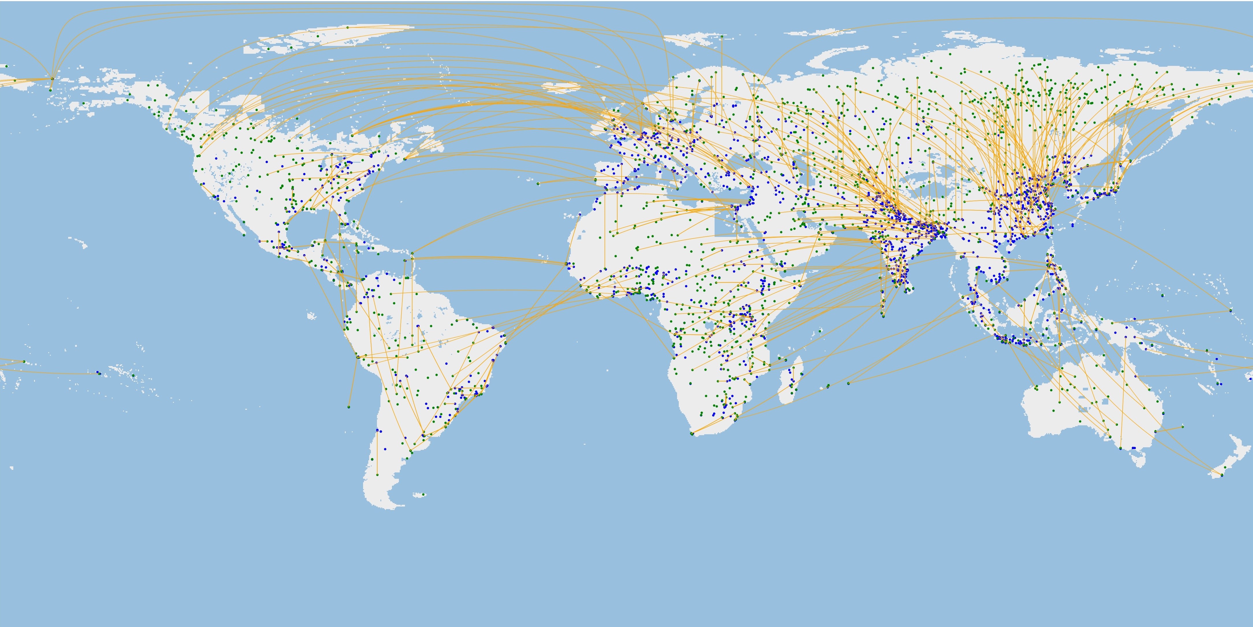
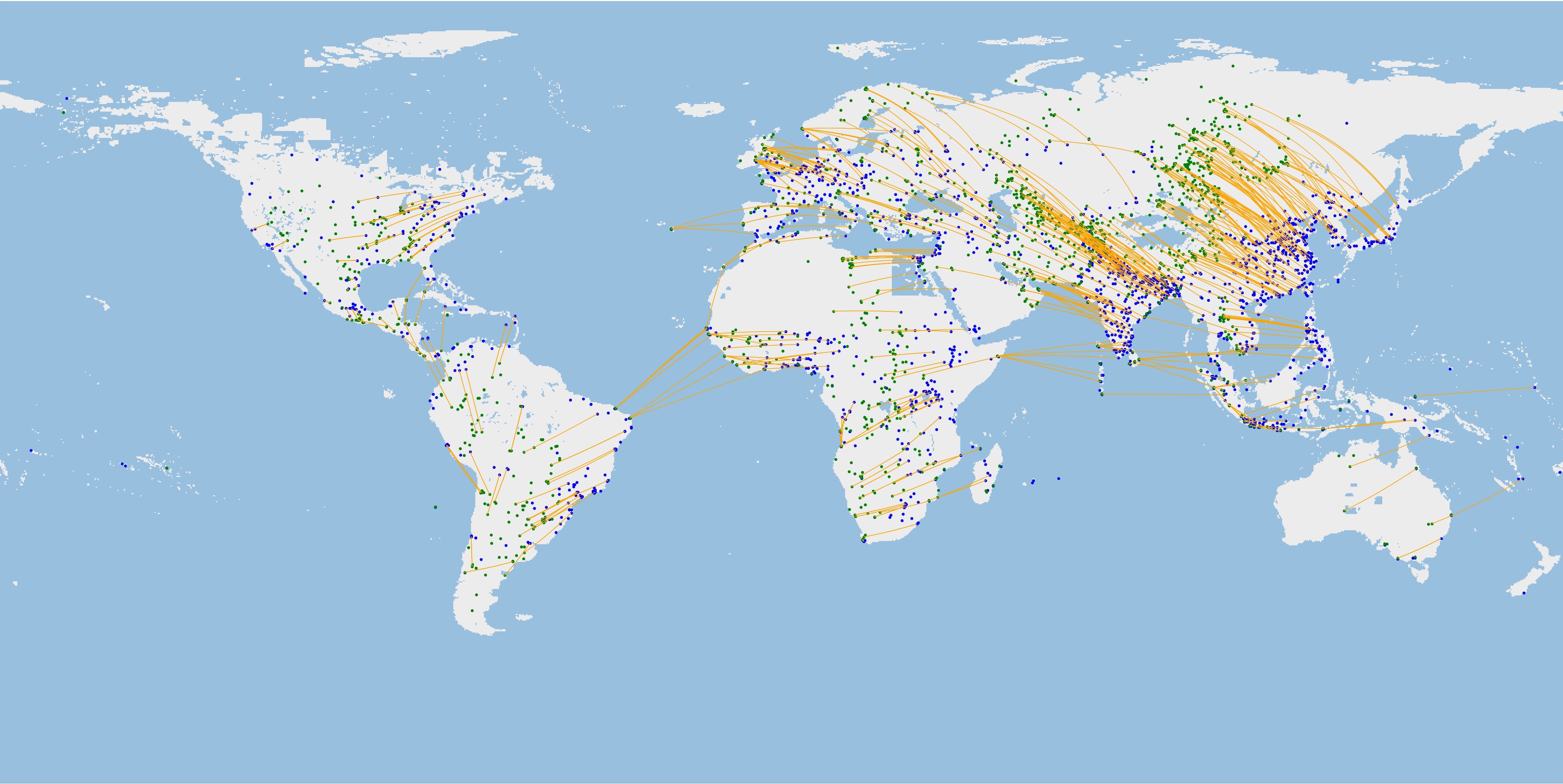
Figure 8: We show our result on top and Perrot et al., (2016) in the bottom. Each figure plots samples from the source distribution $\rho^{\textrm{Sph}}_{a}$ (blue) and samples from the pushforwarded distribution $T_{\theta\sharp}\rho^{\textrm{Sph}}_{a}$ (green). We also demonstrates the computed transport map (orange) for the first $500$ randomly generated points from source $\rho_{a}^{\textrm{Sph}}$ to target $\rho_{b}^{\textrm{Sph}}$.

7 Conclusion and limitation

In this paper we present a novel method to compute Monge map between two given distributions with flexible transport cost functions. In particular, we consider applying Lagrange multipliers on the Monge problem, which leads to a max-min saddle point problem. By further introducing neural networks into our optimization, we obtain a scalable algorithm that can handle most general costs and even the case where the dimensions of marginals are unequal. Our scheme is shown to be effective through a series of experiments with high dimensional large scale datasets, where we only assume the unpaired samples from marginals are accessible. It will become an useful tool for machine learning applications such as domain adaption, and image restoration that require transforming data distributions. In the future, it is promising to specialize our method to structured data, such as time series, graphs, and point clouds.

Limitation

We observe that when the target distribution is a discrete distribution that is with fixed support, our method tends to be more unstable. We conjecture this is because the network parameterization of discriminator is too complex for this type of uncomplicated target distribution.

Appendix A Backgrounds of optimal transport problems

In this work, we assume that the cost function $c$ satisfies the following three conditions

$$c\textrm{ is bounded from below, i.e., there exists }\underaccent{\bar}{c}\in\mathbb{R},\textrm{ such that }c\geq\underaccent{\bar}{c}\textrm{ on }\mathbb{R}^{n}\times\mathbb{R}^{m};$$ (9)

$$c~{}~{}\textrm{is {locally Lipschitz} and {superdifferentiable} everywhere};$$ (10)

$$\partial_{x}c(x,\cdot)~{}~{}\textrm{is injective for any}~{}x\in\mathbb{R}^{n}.$$ (11)

Here we define the local Lipschitz property and superdifferentiablity as follows.

Definition 1 (Locally Lipschitz).

Let $U\subset\mathbb{R}^{n}$ be open and let $f:\mathbb{R}^{n}\rightarrow\mathbb{R}$ be given. Then

(1) $f$ is Lipschitz if there exists $L<\infty$ such that

$$\forall x,z\in\mathbb{R}^{n},\quad|f(z)-f(x)|\leq L|x-z|.$$

(2) $f$ is said to be locally Lipschitz if for any $x_{0}\in\mathbb{R}^{n}$, there is a neighbourhood $O$ of $x_{0}$ in which $f$ is Lipschitz.

Definition 2 (Superdifferentiablity).

For function $f:\mathbb{R}^{n}\rightarrow\mathbb{R}$, we say $f$ is superdifferentiable at $x$, if there exists $p\in\mathbb{R}^{n}$, such that

$$f(z)\geq f(x)+\langle p,z-x\rangle+o(|z-x|).$$

Recall that the Kantorovich dual problem of the primal OT problem (2) is formulated as

$$K(\rho_{a},\rho_{b})=\sup_{\begin{subarray}{c}\text{$(\psi,\phi)\in L^{1}(\rho_{a})\times L^{1}(\rho_{b})$}\\ \text{$\phi(y)-\psi(x)\leq c(x,y)~{}\forall~{}x\in\mathbb{R}^{n},y\in\mathbb{R}^{m}$}\end{subarray}}\left\{\int_{\mathbb{R}^{m}}\phi(y)\rho_{b}(y)~{}dy-\int_{\mathbb{R}^{n}}\psi(x)\rho_{a}(x)~{}dx\right\}.$$

We denote the optimal value of this dual problem as $K(\rho_{a},\rho_{b})$.

It is not hard to tell that the above dual problem is equivalent to any of the following two problems

$$\sup_{\psi\in L^{1}(\rho_{a})}\left\{\int_{\mathbb{R}^{m}}\psi^{c,+}(y)\rho_{b}(y)~{}dy-\int_{\mathbb{R}^{n}}\psi(x)\rho_{a}(x)~{}dx\right\},$$ (12)

$$\sup_{\phi\in L^{1}(\rho_{b})}\left\{\int_{\mathbb{R}^{m}}\phi(y)\rho_{b}(y)~{}dy-\int_{\mathbb{R}^{n}}\phi^{c,-}(x)\rho_{a}(x)~{}dx\right\}.$$ (13)

Here the $c-$transform $\psi^{c,+}$, $\phi^{c,-}$ are defined via infimum/supremum convolution as: $\psi^{c,+}(y)=\inf_{x}(\psi(x)+c(x,y))$ and $\phi^{c,-}(x)=\sup_{y}(\phi(y)-c(x,y))$. If we denote $\psi_{*},\phi_{*}$ as the optimal solutions to (12), (13) respectively. Then both $(\psi_{*},\psi_{*}^{c,+})$ and $(\phi^{c,-}_{*},\phi_{*})$ are the optimal solutions to (3); $\psi_{*}^{c,+}$, $\phi_{*}^{c,-}$ are also solutions to (13), (12) respectively.

The following theorem states the equivalent relationship between the primal OT problem (2) and its Kantorovich dual (3). The proof for a more general version can be found in Theorem 5.10 of Villani, (2008).

Theorem 5 (Kantorovich Duality).

Suppose $c$ is a cost function defined on $\mathbb{R}^{n}\times\mathbb{R}^{m}$ and satisfies (9). Recall that $C(\rho_{a},\rho_{b})$ denotes the infimum value of (2) and $K(\rho_{a},\rho_{b})$ denotes the maximum value of (3) (or equivalently, (12), (13)). Then $C(\rho_{a},\rho_{b})=K(\rho_{a},\rho_{b})$.

The following result states the existence and uniqueness of the optimal solution to the Monge problem. It also reveals the relation between the optimal map $T_{*}$ of (1) and the optimal transport plan $\pi_{*}$ of (2). It is a simplified version of Theorem 10.28 combined with Remark 10.33 taken from Villani, (2008).

Theorem 1 (Existence, uniqueness and characterization of the optimal Monge map).

Suppose the cost $c$ satisfies (9), (10), (11), we further assume that $\rho_{a}$ and $\rho_{b}$ are compactly supported and $\rho_{a}$ is absolute continuous with respect to the Lebesgue measure on $\mathbb{R}^{n}$. Then there exists unique-in-law transport map $T_{*}$ solving the Monge problem (1). And the joint distribution $(\textrm{Id},T_{*})_{\sharp}\rho_{a}$ on $\mathbb{R}^{n+m}$ is the optimal transport plan of the general OT problem (2). Furthermore, there exists $\psi_{*}$ differentiable $\rho_{a}$ almost surely, and $\nabla\psi_{*}(x)+\partial_{x}c(x,T_{*}(x))=0$, $\rho_{a}$ almost surely.

Appendix B Relation between our method and generative adversarial networks

It is worth pointing out that our scheme and Wasserstein Generative Adversarial Networks (WGAN) Arjovsky et al., (2017) are similar in the sense that they are both doing minimization over the generator/map and maximization over the discriminator/dual potential. However, there are two main distinctions between them. Such differences are not reflected from the superficial aspects such as the choice of reference distributions $\rho_{a}$, but come from the fundamental logic hidden behind the algorithms.

• We want to first emphasize that the mechanisms of two algorithms are different: Typical Wasserstein GANs (WGAN) are usually formulated as

  $$\min_{G}\underbrace{\max_{\|D\|_{\textrm{Lip}\leq 1}}\int D(y)\rho_{b}(y)dy-\int D(G(x))\rho_{a}(x)dx}_{1-\textrm{Wasserstein distance }W_{1}(G_{\sharp}\rho_{a},\rho_{b})}$$ (14)

  and ours reads

  $$\underbrace{\max_{f}\min_{T}\int f(y)\rho_{b}(y)dy-\int f(T(x))\rho_{a}(x)dx+\int c(X,T(x))\rho_{a}(x)dx}_{\textrm{general Wasserstein distance }C_{\textrm{Monge}}(\rho_{a},\rho_{b})}$$ (15)

  The inner maximization of (14) computes $W_{1}$ distance via Kantorovich duality and the outer loop minimize the $W_{1}$ gap between desired $\rho_{b}$ and $G_{\sharp}\rho_{a}$; However, the logic behind our scheme (15) is different: the inner optimization computes for the $c-$transform of $f$, i.e. $f^{c,-}(x)=\sup_{\xi}(f(\xi)-c(x,\xi))$; And the outer maximization computes for the Kantorovich dual problem $C(\rho_{a},\rho_{b})=\sup_{f}\left\{\int f(y)\rho_{b}(y)dy-\int f^{c,-}(x)\rho_{a}(x)dx\right\}$.

  Even under $W_{1}$ circumstance, one can verify the intrinsic difference between two proposed methods: when setting the cost $c(x,y)=\|x-y\|$, and $\rho_{a}=G\sharp\rho_{a}$ in (15), the entire "max-min" optimization of (15) (underbraced part) is equivalent to the inner maximization problem of (14) (underbraced part), but not for the entire saddle point scheme.

  It is also important to note that WGAN aims to minimize the distance between generated distribution and the target distribution and the ideal value for (14) is $0$. On the other hand, one of our goal is to estimate the optimal transport distance between the initial distribution $\rho_{a}$ and the target distribution $\rho_{b}$. Thus the ideal value for (15) should be $C(\rho_{a},\rho_{b})$, which is not $0$ in most of the cases.

• We then argue about the optimality of the computed map $G$ and $T$: In (14), one is trying to obtain a map $G$ by minimizing $W_{1}(\rho_{b},G_{\sharp}\rho_{a})$ w.r.t. $G$, and hopefully, $G_{\sharp}\rho_{a}$ can approximate $\rho_{b}$ well. However, there isn’t any restriction exerted on $G$, thus one can not expect the computed $G$ to be the optimal transport map between $\rho_{a}$ and $\rho_{b}$; On the other hand, in (15), we not only compute $T$ such that $T_{\sharp}\rho_{a}$ approximates $\rho_{b}$ , but also compute for the optimal $T$ that minimizes the transport cost $\mathbb{E}_{\rho_{a}}[c(X,T(X))]$. In (15), the computation of $T$ is naturally incorporated in the max-min scheme and there exists theoretical result (recall Theorem 2 in the paper) that guarantees $T$ to be the optimal transport map.

In summary, even though the formulation of both algorithms are similar, the designing logic (minimizing distance vs computing distance itself) and the purposes (computing arbitary pushforward map vs computing the optimal map) of the two methods are distinct. Thus the theoretical and empirical study of GANs cannot be trivially translated to proposed method. In addition to the above discussions, we should also refer the readers to Gazdieva et al., (2022), in which a comparison between a similar saddle point method and the regularized GANs are made in section 6.2 and summarized in Table 1.

Appendix C Proof of Consistency

We firstly prove the following result on the consistency of our proposed method.

Theorem 2 (Consistency with $\bar{T}_{\sharp}\rho_{a}=\rho_{b}$).

Suppose the max-min problem (4) admits at least one saddle point solution. We denote it as $(\bar{T},\bar{f})$. Under the assumption $\bar{T}_{\sharp}\rho_{a}=\rho_{b}$, we have

• $\bar{f}$ is an optimal solution $\phi$ to the Kantorovich dual problem (3). Or equivalently, $\bar{f}$ is an optimal solution to (13);

• The optimal solution to the Monge problem (1) exists, and $\bar{T}$ is an optimal solution, i.e. $\bar{T}$ is the Monge map.

• Furthermore, $\mathcal{L}(\bar{T},\bar{f})=C_{\textrm{Monge}}(\rho_{a},\rho_{b})$.

Proof of Theorem 2.

First one can verify the following

$$\inf_{T}\mathcal{L}(T,f)= -\int_{\mathbb{R}^{n}}\sup_{\xi}\{f(\xi)-c(x,\xi)\}\rho_{a}(x)dx+\int_{\mathbb{R}^{m}}f(y)\rho_{b}(y)dy$$

$$= \int_{\mathbb{R}^{m}}f(y)\rho_{b}(y)dy-\int_{\mathbb{R}^{n}}f^{c,-}(x)\rho_{a}(x)dx,$$ (16)

Then the max-min problem $\sup_{f}\inf_{T}\mathcal{L}(T,f)$ can be formulated as

$$\sup_{f}\left\{\int_{\mathbb{R}^{m}}f(y)\rho_{b}(y)dy-\int_{\mathbb{R}^{n}}f^{c,-}(x)\rho_{a}(x)dx\right\}.$$

This is exactly the Kantorovich dual problem (13). Since $(\bar{T},\bar{f})$ is the saddle point, $\bar{f}$ is an optimal solution to (13). This verifies the first assertion of the theorem.

On the other hand, at the saddle point $(\bar{T},\bar{f})$, we have

$$\quad\bar{T}(x)\in\textrm{argmax}_{\xi\in\mathbb{R}^{m}}\{\bar{f}(\xi)-c(x,\xi)\},~{}\rho_{a}~{}\textrm{almost surely}.$$

This leads to

$$f^{c,-}_{*}(x)=\bar{f}(\bar{T}(x))-c(x,\bar{T}(x)),~{}\rho_{a}~{}\textrm{almost surely}.$$

Then we have

$$\int_{\mathbb{R}^{n}}c(x,\bar{T}(x))\rho_{a}(x)~{}dx =\int_{\mathbb{R}^{n}}\bar{f}(\bar{T}(x))\rho_{a}(x)~{}dx-\int_{\mathbb{R}^{n}}\bar{f}^{c,-}(x)\rho_{a}(x)~{}dx$$

$$=\int_{\mathbb{R}^{m}}\bar{f}(y)\rho_{b}(y)~{}dy-\int_{\mathbb{R}^{n}}\bar{f}^{c,-}(x)\rho_{a}(x)~{}dx$$

$$=\int_{\mathbb{R}^{n}\times\mathbb{R}^{m}}[\bar{f}(y)-f^{c,-}_{*}(x)]d\pi(x,y)\leq\int_{\mathbb{R}^{n}\times\mathbb{R}^{m}}c(x,y)d\pi(x,y)$$

for any $\pi\in\Pi(\rho_{a},\rho_{b})$. Here the second equality is due to the assumption $T_{*\sharp}\rho_{a}=\rho_{b}$. The last inequality is due to the definition of $f^{c,-}_{*}(x)=\sup_{y}\{\bar{f}(y)-c(x,y)\}$.

We now take the infimum value of $\int_{\mathbb{R}^{n}\times\mathbb{R}^{m}}cd\pi$ and we obtain

$$\int_{\mathbb{R}^{n}}c(x,\bar{T}(x))\rho_{a}(x)~{}dx\leq C(\rho_{a},\rho_{b}),$$ (17)

Now, for any transport map $T$ satisfying $T_{\sharp}\rho_{a}=\rho_{b}$, by denoting $\pi=(\textrm{Id},T)_{\sharp}\rho_{a}$, we have

$$\int_{\mathbb{R}^{n}}c(x,T(x))\rho_{a}(x)~{}dx=\int_{\mathbb{R}^{n}\times\mathbb{R}^{m}}c(x,y)d\pi(x,y)\geq C(\rho_{a},\rho_{b}).$$ (18)

Combining (17) and (18), we obtain

$$\int_{\mathbb{R}^{n}}c(x,\bar{T}(x))\rho_{a}(x)dx\leq\int_{\mathbb{R}^{n}}c(x,T(x))\rho_{a}(x)dx,\quad\textrm{for any}~{}T,~{}T_{\sharp}\rho_{a}=\rho_{b}.$$

This indicates the existence of the Monge map, and $\bar{T}$ is the Monge map.

At last, we have

$$\mathcal{L}(\bar{T},\bar{f})=\int_{\mathbb{R}^{n}}c(x,\bar{T}(x))\rho_{a}(x)dx+\int_{\mathbb{R}^{m}}\bar{f}(y)(T_{*\sharp}\rho_{a}-\rho_{b})dy=\int_{\mathbb{R}^{n}}c(x,\bar{T}(x))\rho_{a}(x)~{}dx=C_{\textrm{Monge}}(\rho_{a},\rho_{b}).$$

∎

Without the assumption $\bar{T}_{\sharp}\rho_{a}=\rho_{b}$, we no longer have guarantee on the existence of Monge map $T_{*}$, not to mention the consistency between $\bar{T}$ and $T_{*}$. However, we are still able to show the consistency between the saddle point value $\mathcal{L}(\bar{T},\bar{f})$ and general OT distance $C(\rho_{a},\rho_{b})$.

Theorem 3 (Consistency without $\bar{T}_{\sharp}\rho_{a}=\rho_{b}$).

Proof.

The proof of the first part of this theorem is the same as Theorem 2. Thus it is not hard to verify

$$\sup_{f}\int_{T}\mathcal{L}(T,f)=\sup_{f}\left\{\int_{\mathbb{R}^{m}}f(y)\rho_{b}(y)dy-\int_{\mathbb{R}^{n}}f^{c,-}(x)\rho_{a}(x)dx\right\}=K(\rho_{a},\rho_{b}).$$ (19)

Recall Theorem 5, the optimal value of Kantorovich dual problem equals general OT distance $C(\rho_{a},\rho_{b})$. This proves our assertion. ∎

Remark 3.

Theorem 3 indicates that although for some general cases in which our proposed method (4) fails to compute for a valid transport map $\bar{T}$, (4) is still able to recover the exact optimal transport distance $C(\rho_{a},\rho_{b})$.

More specifically, let us consider the OT problem on $\mathbb{R}$ with $c(x,y)=|x-y|^{2}$ and $\rho_{a}=\delta_{0}$ (point distribution at $0$), $\rho_{b}=\mathcal{N}(0,1)$ (normal distribution). Our method yields

$$\sup_{f}\inf_{T}\left\{|T(0)|^{2}+\int f(y)\rho_{b}(y)dy-f(T(0))\right\}.$$

By setting $\Psi_{0}(y)=|y|^{2}-f(y)$, our max-min problem becomes

$$\sup_{f}\inf_{T}\{\Psi_{0}(T(0))+\int(|y|^{2}-\Psi_{0}(y))\rho_{b}(y)dy\}=\underbrace{\int|y|^{2}\rho_{b}(y)dy}_{=1}+\sup_{\Psi_{0}}\underbrace{\left\{\int[\inf\Psi_{0}-\Psi_{0}(y)]\rho_{b}(y)dy\right\}}_{\leq 0}=1$$

The supreme over $\Psi_{0}$ is obtained when $\Psi_{0}=\textrm{Const}$, i.e., when $f(y)=|y|^{2}+\textrm{Const}$. Thus we have $\sup_{f}\inf_{T}\mathcal{L}(T,f)=1=C(\rho_{a},\rho_{b})$. In such example, although the Monge map does not exist, the proposed method can still capture the exact OT distance.

Appendix D Proof of Posterior Error Estimation

Let us first recall the assumptions on the cost $c(\cdot,\cdot)$, marginals $\rho_{a},\rho_{b}$, and dual variable $f$:

Assumption 4 (on cost $c(\cdot,\cdot)$).

We assume $c\in C^{2}(\mathbb{R}^{d}\times\mathbb{R}^{d})$ is bounded from below. Furthermore, for any $x,y\in\mathbb{R}^{d}$, we assume $\partial_{x}c(x,y)$ is injective w.r.t. $y$; $\partial_{xy}c(x,y)$, as a $d\times d$ matrix, is invertible; and $\partial_{yy}c(x,y)$ is independent of $x$.

Assumption 5 (on marginals $\rho_{a}$, $\rho_{b}$).

We assume that $\rho_{a},\rho_{b}$ are compactly supported on $\mathbb{R}^{d}$, and $\rho_{a}$ is absolutely continuous w.r.t. the Lebesgue measure.

Assumption 6 (on dual variable $f$).

Assume the dual variable $f\in C^{2}(\mathbb{R}^{d})$ is always taken from $c$-concave functions, i.e., there exists certain $\varphi\in C^{2}(\mathbb{R}^{d})$ such that $f(\cdot)=\inf_{x}\{\varphi(x)+c(x,\cdot)\}$ (c.f. Definition 5.7 of Villani, (2008)). Furthermore, we assume that there exists a unique minimizer $x_{y}\in\textrm{argmin}_{x}\{\varphi(x)+c(x,y)\}$ for any $y\in\mathbb{R}^{d}$. And the Hessian of $\varphi(\cdot)+c(\cdot,y)$ at $x_{y}$ is positive definite.

We then introduce the following two notations. We denote

$$\sigma(x,y)=\sigma_{\min}(\partial_{xy}c(x,y))>0$$

as the minimum singular value of $\partial_{xy}c(x,y)$; and

$$\lambda(y)=\lambda_{\max}(\nabla^{2}_{xx}(\varphi(x)+c(x,y))|_{x=x_{y}})>0$$

as the maximum eigenvalue of the Hessian of $\varphi(\cdot)+c(\cdot,y)$ at $x_{y}$.

We denote the duality gaps as

$$\mathcal{E}_{1}(T,f)=\mathcal{L}(T,f)-\inf_{\widetilde{T}}\mathcal{L}(\widetilde{T},f),$$

$$\mathcal{E}_{2}(f)=\sup_{\widetilde{f}}\inf_{\widetilde{T}}\mathcal{L}(\widetilde{T},\widetilde{f})-\inf_{\widetilde{T}}\mathcal{L}(\widetilde{T},f).$$

It is not hard to verify the following lemma:

Lemma 1 (Existence and uniqueness of Monge map under Assumption 1, 2).

Suppose Assumption 1 and 2 hold, then the conditions on $c(\cdot,\cdot)$ and $\rho_{a},\rho_{b}$ mentioned in Theorem 1 are all satisfied. Thus the Monge map $T_{*}$ exists and is unique in law.

We now state the main theorem on error estimation:

Theorem 4 (Posterior Error Enstimation via Duality Gaps).

Suppose Assumption 1, 2 and 3 hold. Let us further assume the max-min problem (4) admits a saddle point $(\bar{f},\bar{T})$ that is consistent with the Monge problem, i.e. $\bar{T}$ equals $T_{*}$, $\rho_{a}$ almost surely. Then there exists a strict positive weight function $\beta(x)>\underset{y\in\mathbb{R}^{m}}{\min}\left\{\frac{\sigma(x,y)}{2\lambda(y)}\right\}$ such that the weighted $L^{2}$ error between computed map $T$ and the Monge map $T_{*}$ is upper bounded by

$$\|T-T_{*}\|_{L^{2}(\beta\rho_{a})}\leq\sqrt{2(\mathcal{E}_{1}(T,f)+\mathcal{E}_{2}(f))}.$$

To prove Theorem 4, we need the following two lemmas:

Lemma 2.

Suppose $n\times n$ matrix $A$ is invertible with minimum singular value $\sigma_{\min}(A)>0$. Also assume $n\times n$ matrix $H$ is self-adjoint and satisfies $\lambda I_{n}\succeq H\succ O_{n}$. Then $A^{\top}H^{-1}A\succeq\frac{\sigma_{\min}(A)^{2}}{\lambda}I_{n}$.

Proof of Lemma 2 .

One can first verify that $H^{-1}\succeq\frac{1}{\lambda}I_{n}$ by digonalizing $H^{-1}$. To prove this lemma, we only need to verify that for arbitrary $v\in\mathbb{R}^{n}$,

$$v^{\top}A^{\top}H^{-1}Av=(Av)^{\top}H^{-1}Av\geq\frac{|Av|^{2}}{\lambda}\geq\frac{\sigma_{\min}(A)^{2}}{\lambda}|v|^{2}$$

Thus $A^{\top}H^{-1}A-\frac{\sigma_{\min}(A)^{2}}{\lambda}I_{n}$ is positive-semidefinite. ∎

The following lemma is crucial for proving our results, it analyzes the concavity of the target function $f(\cdot)-c(\cdot,y)$ with $f$ is $c$-concave.

Lemma 3 (Concavity of $f(\cdot)-c(x,\cdot)$ if $f$ $c$-concave).

Suppose the cost function $c(x,y)$ and $f$ satisfy the conditions mentioned in Theorem 4. Denote the function $\Psi_{x}(y)=f(y)-c(x,y)$, keep all notations defined in Theorem 4, then we have

$$\nabla^{2}\Psi_{x}(y)\preceq-\frac{\sigma(x,y)^{2}}{\lambda(y)}I_{n}.$$

Proof of Lemma 3.

First, we notice that $f$ is $c$-convex, thus, there exists $\varphi$ such that $f(y)=\inf_{x}\{\varphi(x)+c(x,y)\}$. Let us also denote $\Phi(x,y)=\varphi(x)+c(x,y)$.

Now for a fixed $y\in\mathbb{R}^{n}$, We pick one

$$x_{y}\in\textrm{argmin}_{x}\left\{\varphi(x)+c(x,y)\right\}$$

Since we assumed that $\varphi\in C^{2}(\mathbb{R}^{n})$ and $c\in C^{2}(\mathbb{R}^{n}\times\mathbb{R}^{n})$, we have

$$\partial_{x}\Phi(x_{y},y)=\nabla\varphi(x_{y})+\partial_{x}c(x_{y},y)=0$$ (20)

Now recall Assumption 3, $\partial_{xx}^{2}\Phi(x_{y},y)$ is positive definite, thus is also invertible. We can now apply the implicit function theorem to show that the equation $\partial_{x}\Phi(x,y)=0$ determines an implicit function $x(\cdot)$, which satisfies $x(y)=x_{y}$ in a small neighbourhood $U\subset\mathbb{R}^{n}$ containing $y$. Furthermore, one can show that $x(\cdot)$ is continuously differentiable at $y$. We will denote $x_{y}$ as $x(y)$ in our following discussion.

Now differentiating (20) with respect to $y$ yields

$$\partial_{xx}^{2}\Phi(x(y),y)\nabla x(y)+\partial_{xy}^{2}c(x(y),y)=0$$ (21)

On one hand, (21) tells us

$$\nabla x(y)=-\partial_{xx}\Phi(x(y),y)^{-1}\partial_{xy}c(x(y),y).$$ (22)

Now we directly compute

$$\nabla^{2}\Psi_{x}(y)=\nabla^{2}f(y)-\partial_{yy}^{2}c(x,y).$$ (23)

in order to compute $\nabla^{2}f(y)$, we first compute $\nabla f(y)$

$$\nabla f(y)=\nabla(\varphi(x(y))+c(x(y),y))=\partial_{y}c(x(y),y).$$ (24)

the second equality is due to the envelope theorem Afriat, (1971). Then $\nabla^{2}f(y)$ can be computed as

$$\nabla^{2}f(y)=\partial_{yx}c(x(y),y)\nabla x(y)+\partial_{yy}c(x(y),y).$$ (25)

Plugging (22) into (25), recall (23), this yields

$$\nabla^{2}\Psi_{x}(y)=-\partial_{yx}c(x(y),y)\partial_{xx}\Phi(x(y),y)^{-1}\partial_{xy}c(x(y),y)+\partial_{yy}^{2}c(x(y),y)-\partial_{yy}^{2}c(x,y).$$

Recall the Assumption 1, notice that $c\in C^{2}(\mathbb{R}^{n}\times\mathbb{R}^{n})$, by symmetry of second derivatives, one can verify $\partial_{xy}c^{\top}=\partial_{yx}c$; Since $\partial_{yy}c(x,y)$ is independent of $x$, one has $\partial_{yy}^{2}c(x(y),y)-\partial_{yy}^{2}c(x,y)=0$. Thus we obtain

$$\nabla^{2}\Psi_{x}(y)=-\partial_{xy}^{\top}c(x(y),y)\partial_{xx}\Phi(x(y),y)^{-1}\partial_{xy}c(x(y),y).$$ (26)

By (LABEL:boundness_of_Phi), $\lambda(y)I_{n}\succeq\partial_{xx}\Phi(x(y),y)\succ O_{n}$. Recall that $\sigma_{\min}(\partial_{xy}c(x,y))=\sigma(x,y)$. Now we apply lemma 2 to (26), this yields

$$\nabla^{2}\Psi_{x}(y)\preceq-\frac{\sigma(x,y)^{2}}{\lambda(y)}I_{n}.$$

∎

Now we prove the main result of Theorem 4:

Proof of Theorem 4.

In this proof, we denote $\int$ as $\int_{\mathbb{R}^{d}}$ for simplicity.

We first recall

$$\mathcal{L}(T,f)= \int c(x,T(x))\rho_{a}(x)~{}dx+\int f(y)\rho_{b}(y)~{}dy-\int f(T(x))\rho_{a}(x)~{}dx$$

$$= \int f(y)\rho_{b}(y)~{}dy-\int(f(T(x))-c(x,T(x)))\rho_{a}(x)dx,$$

then we write

$$\mathcal{E}_{1}(T,f)=\mathcal{L}(T,f)-\inf_{\widetilde{T}}\mathcal{L}(\widetilde{T},f)=-\int[f(T(x))-c(x,T(x))]\rho_{a}~{}dx+\sup_{\widetilde{T}}\left\{\int[f(\widetilde{T}(x))-c(x,\widetilde{T}(x))]\rho_{a}~{}dx\right\}$$

We denote

$$T_{f}(x)=\textrm{argmax}_{y}\{f(y)-c(x,y)\}=\textrm{argmax}_{y}\{\Psi_{x}(y)\},$$ (27)

recall that we denote $\Psi_{x}(y)=f(y)-c(x,y)$, then we have

$$\nabla\Psi_{x}(T_{f}(x))=0.$$ (28)

One can also write:

$$\mathcal{E}_{1}(T,f)= \int[(f(T_{f}(x))-c(x,T_{f}(x)))-(f(T(x))-c(x,T(x)))]$$

$$= \int[\Psi_{x}(T_{f}(x))-\Psi_{x}(T(x))]\rho_{a}(x)~{}dx$$

For any $x\in\mathbb{R}^{d}$, since $\Psi_{x}(\cdot)\in C^{2}(\mathbb{R}^{n})$, and according to the previous Lemma 3, we have

$$\Psi_{x}(T(x))-\Psi_{x}(T_{f}(x))=\nabla\Psi_{x}(T_{f}(x))(T(x)-T_{f}(x))+\frac{1}{2}(T(x)-T_{f}(x))^{\top}\nabla^{2}\Psi_{x}(\omega(x))(T(x)-T_{f}(x))$$

with $\omega(x)=(1-\theta_{x})T(x)+\theta_{x}T_{f}(x)$ for certain $\theta_{x}\in[0,1]$. By (28) and Lemma 3, we have

$$\Psi_{x}(T(x))-\Psi_{x}(T_{f}(x))\leq-\frac{\sigma(x,\omega(x))^{2}}{2\lambda(\omega(x))}|T(x)-T_{f}(x)|^{2}.$$

Thus we have:

$$\mathcal{E}_{1}(T,f)=\int[\Psi_{x}(T_{f}(x))-\Psi_{x}(T(x))]\rho_{a}(x)~{}dx\geq\int\frac{\sigma(x,\omega(x))^{2}}{2\lambda(\omega(x))}|T(x)-T_{f}(x)|^{2}\rho_{a}(x)~{}dx$$ (29)

On the other hand, recall a saddle point solution of our max-min problem (4) is denoted as $(\bar{T},\bar{f})$. Then we have

$$\sup_{f}\inf_{T}\mathcal{L}(T,f)=\int c(x,\bar{T}(x))\rho_{a}~{}dx-\int f(y)(\bar{T}_{\sharp}\rho_{a}-\rho_{b})dy=\int c(x,\bar{T}(x))\rho_{a}~{}dx,$$

the second equality is due to the assumption on the consistency between $\bar{T}$ and Monge map $T_{*}$, thus $\bar{T}_{\sharp}\rho_{a}=\rho_{b}$.

Thus we have

$$\mathcal{E}_{2}(f)= \int c(x,\bar{T}(x))\rho_{a}~{}dx-\inf_{\widetilde{T}}\left(\int c(x,\widetilde{T}(x))\rho_{a}(x)dx+\int f(y)\rho_{b}(y)~{}dy-\int f(\widetilde{T}(x))\rho_{a}(x)dx\right)$$

$$= -\int f(\bar{T}(x))-c(x,\bar{T}(x))\rho_{a}~{}dx+\sup_{\widetilde{T}}\int(f(\widetilde{T}(x))-c(x,\widetilde{T}(x)))\rho_{a}(x)dx.$$

The second equality is due to $\bar{T}_{\sharp}\rho_{a}=\rho_{b}$. Similar to the previous treatment, we have

$$\mathcal{E}_{2}(f)=\int[\Psi_{x}(T_{f}(x))-\Psi_{x}(\bar{T}(x))]\rho_{a}(x)~{}dx$$

Apply similar analysis as before, we obtain

$$\mathcal{E}_{2}(f)\geq\int\frac{\sigma(x,\xi(x))^{2}}{2\lambda(\xi(x))}|\bar{T}(x)-T_{f}(x)|^{2}\rho_{a}(x)~{}dx$$ (30)

with $\xi(x)=(1-\tau_{x})\bar{T}(x)+\tau_{x}T_{f}(x)$ for certain $\tau_{x}\in[0,1]$. Since $\bar{T}=T_{*}$, $\rho_{a}$ almost surely, (31) leads to

$$\mathcal{E}_{2}(f)\geq\int\frac{\sigma(x,\xi(x))^{2}}{2\lambda(\xi(x))}|T_{*}(x)-T_{f}(x)|^{2}\rho_{a}(x)~{}dx$$ (31)

Now we set

$$\beta(x)=\min\left\{\frac{\sigma(x,\omega(x))}{2\lambda(\omega(x))},\frac{\sigma(x,\xi(x))}{2\lambda(\xi(x))}\right\},$$ (32)

combining (29) and (31), we obtain

$$\mathcal{E}_{1}(T,f)+\mathcal{E}_{2}(f) \geq\int\beta(x)(|T(x)-T_{f}(x)|^{2}+|T_{*}(x)-T_{f}(x)|^{2})\rho_{a}~{}dx$$

$$\geq\int\frac{\beta(x)}{2}|T(x)-T_{*}(x)|^{2}\rho_{a}~{}dx$$

This leads to $\|T-T_{*}\|_{L^{2}(\beta\rho_{a})}\leq\sqrt{2(\mathcal{E}_{1}(T,f)+\mathcal{E}_{2}(f))}$.

∎

Appendix E Additional results

E.1 Synthetic datasets

Learning with unequal dimensions

Our algorithm framework enjoys a distinguishing quality that it can learn the map from a lower dimension space $\mathbb{R}^{n}$ to a manifold in a higher dimension space $\mathbb{R}^{m}(n\leq m)$. In this scenario, we make the input dimension of neural network $T$ to be $n$ and output dimension to be $m$. In case the cost function $c(x,y)$ requires dimensions are $x$ and $y$ are equal dimensional, we patch zeros behind each sample $X\sim\rho_{a}$ and complement to a counterpart sample $\widetilde{X}=[X;{\bm{0}}]$, where dimension of ${\bm{0}}$ is $m-n$. And the targeted min-max problem is replaced by

$$\max_{\eta}\min_{\theta}\frac{1}{N}\sum_{k=1}^{N}c({\widetilde{X}_{k}},T_{\theta}({{X}_{k}}))-f_{\eta}(T_{\theta}({{X}_{k}}))+f_{\eta}({Y_{k}}).$$

In Figure 9, we conduct one experiment for $n=1$ and $m=2$. The incomplete ellipse is a 1D manifold and our algorithm is able to learn a symmetric map from $\mathcal{N}(0,1)$ towards it.

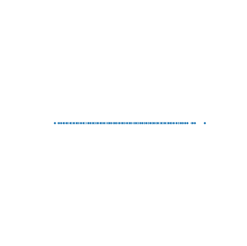
(a) $\rho_{a}$

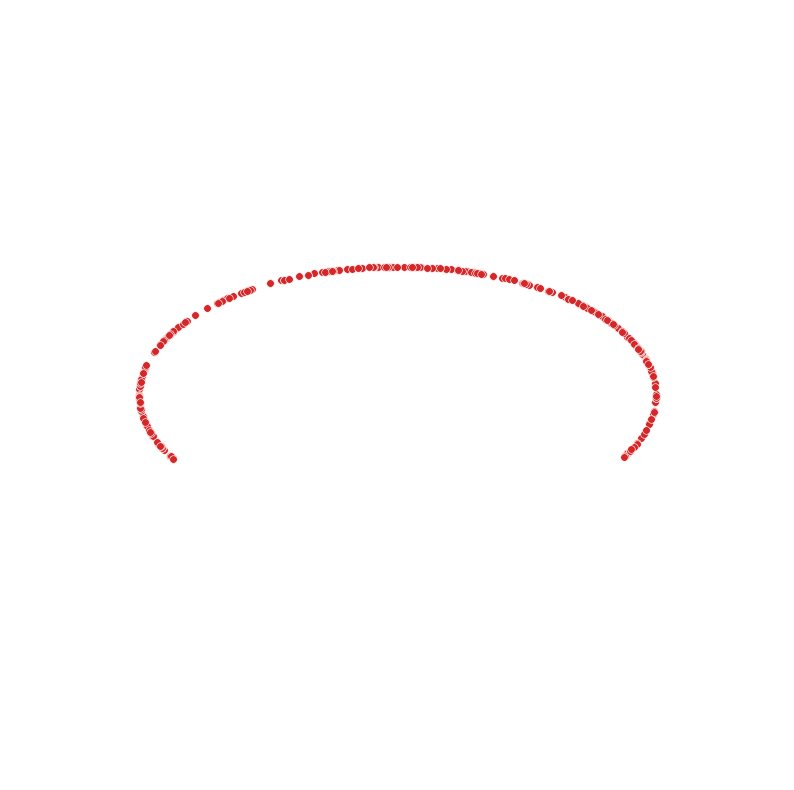
(b) $\rho_{b}$

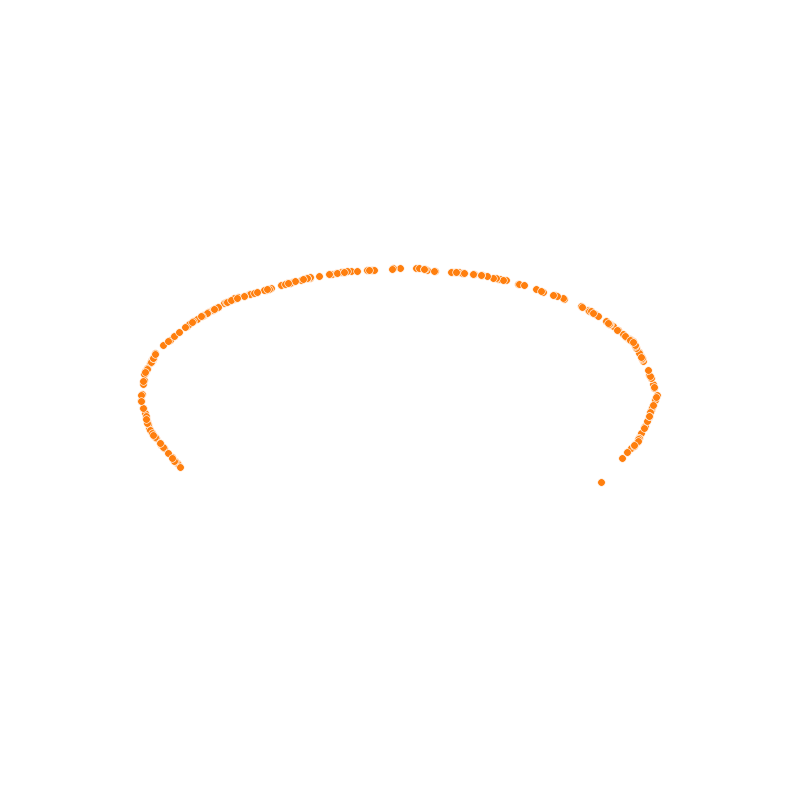
(c) $T\sharp\rho_{a}$

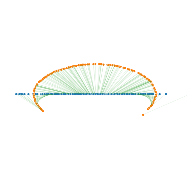
(d) $T(\cdot)$ map

Figure 9: Qualitative results for learning unequal dimension maps. $\rho_{a}$ for two examples are both $\mathcal{N}(0,1)$, and $\rho_{b}$ are uniformly distributed on a incomplete ellipse and a ball respectively.

Decreasing function as the cost

We consider the cost function $c(x,y)=\phi(|x-y|)$ with $\phi$ as a monotonic decreasing function. We test our algorithm for a specific example $\phi(s)=\frac{1}{s^{2}}$. In this example, we compute for the optimal Monge map from $\rho_{a}$ to $\rho_{b}$ with $\rho_{a}$ as a uniform distribution on $\Omega_{a}$ and $\rho_{b}$ as a uniform distribution on $\Omega_{b}$, where we define

$$\Omega_{a}=\{(x_{1},x_{2})~{}|~{}6^{2}\geq x_{1}^{2}+x_{2}^{2}\geq 4^{2}\},\quad\Omega_{b}=\{(x,x_{2})~{}|~{}2^{2}\geq x_{1}^{2}+x_{2}^{2}\geq 1^{2}\}.$$

We also compute the same problem for $L^{2}$ cost. Figure 10 shows the transported samples as well as the differences between two cost functions.

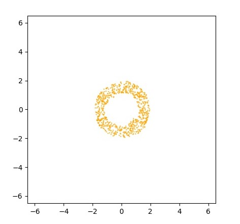
(a)

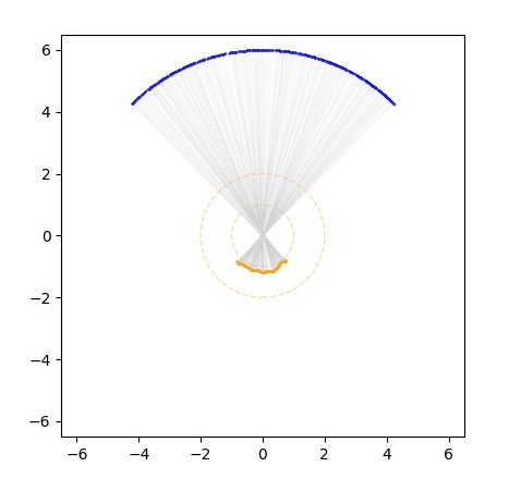
(b)

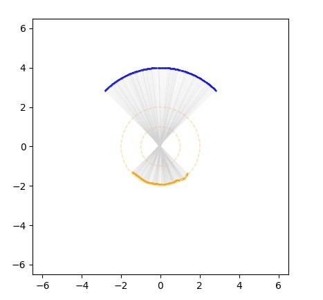
(c)

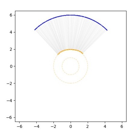
(d)

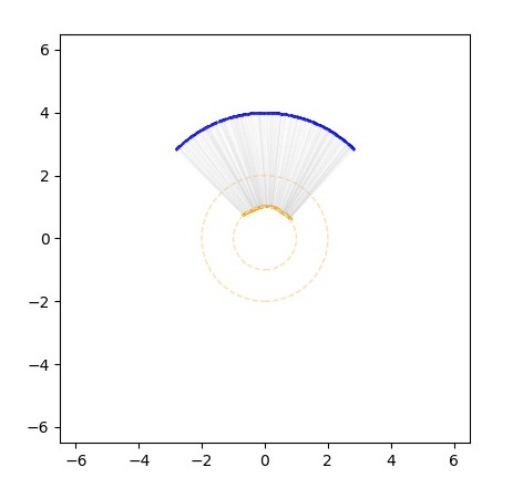
(e)

Figure 10: (a) samples of computed $T_{\sharp}\rho_{a}$; $c(x,y)=\frac{1}{|x-y|^{2}}$: Computed Monge map of quarter circles with radius $6$ (subplot b) and radius $4$ (subplot c); $c(x,y)=|x-y|^{2}$: Computed Monge map of quarter circles with radius $6$ (subplot d) and radius $4$ (subplot e).

Uniform distribution on sphere

For a given sphere $S$ with radius $R$, for any two points $x,y\in S$, we define the distance $d(x,y)$ as the length of the geodesic joining $x$ and $y$. Now for given $\rho_{a}$, $\rho_{b}$ defined on $S$, we consider solving the following Monge problem on $S$

$$\min_{T,~{}T_{\sharp}\rho_{a}=\rho_{b}}\int_{S}d(x,T(x))\rho_{a}(x)~{}dx.$$ (33)

Such sphere OT problem can be transferred to an OT problem defined on angular domain $D=[0,2\pi)\times[0,\pi]$, to be more specific, we consider $(\theta,\phi)$ ($\theta\in[0,2\pi)$, $\phi\in[0,\pi]$) as the azimuthal and polar angle of the spherical coordinates. For two points $x=(R\sin\phi_{1}\cos\theta_{1},R\sin\phi_{1}\sin\theta_{1},R\cos\phi_{1})$, $y=(R\sin\phi_{2}\cos\theta_{2},R\sin\phi_{2}\sin\theta_{2},R\cos\phi_{2})$ on $S$, the geodesic distance

$$d(x,y)=c((\theta_{1},\phi_{1}),(\theta_{2},\phi_{2}))=R\cdot\arccos(\sin\phi_{1}\sin\phi_{2}\cos(\theta_{2}-\theta_{1})+\cos\phi_{1}\cos\phi_{2}).$$

Denote the corresponding distribution of $\rho_{a},\rho_{b}$ on $D$ as $\hat{\rho}_{a},\hat{\rho}_{b}$, now (33) can also be formulated as

$$\min_{\hat{T},\hat{T}_{\sharp}\hat{\rho}_{a}=\hat{\rho}_{b}}\int c((\theta,\phi),\hat{T}(\theta,\phi))\hat{\rho}_{a}~{}d\theta d\phi.$$ (34)

We set $\hat{\rho}_{a}=U([0,2\pi])\otimes U([0,\frac{\pi}{4}])$ and $\hat{\rho}_{b}=U([0,2\pi])\otimes U([\frac{3\pi}{4},\pi])$. We apply our algorithm to solve (34) and then translate our computed Monge map back to the sphere $S$ to obtain the following results

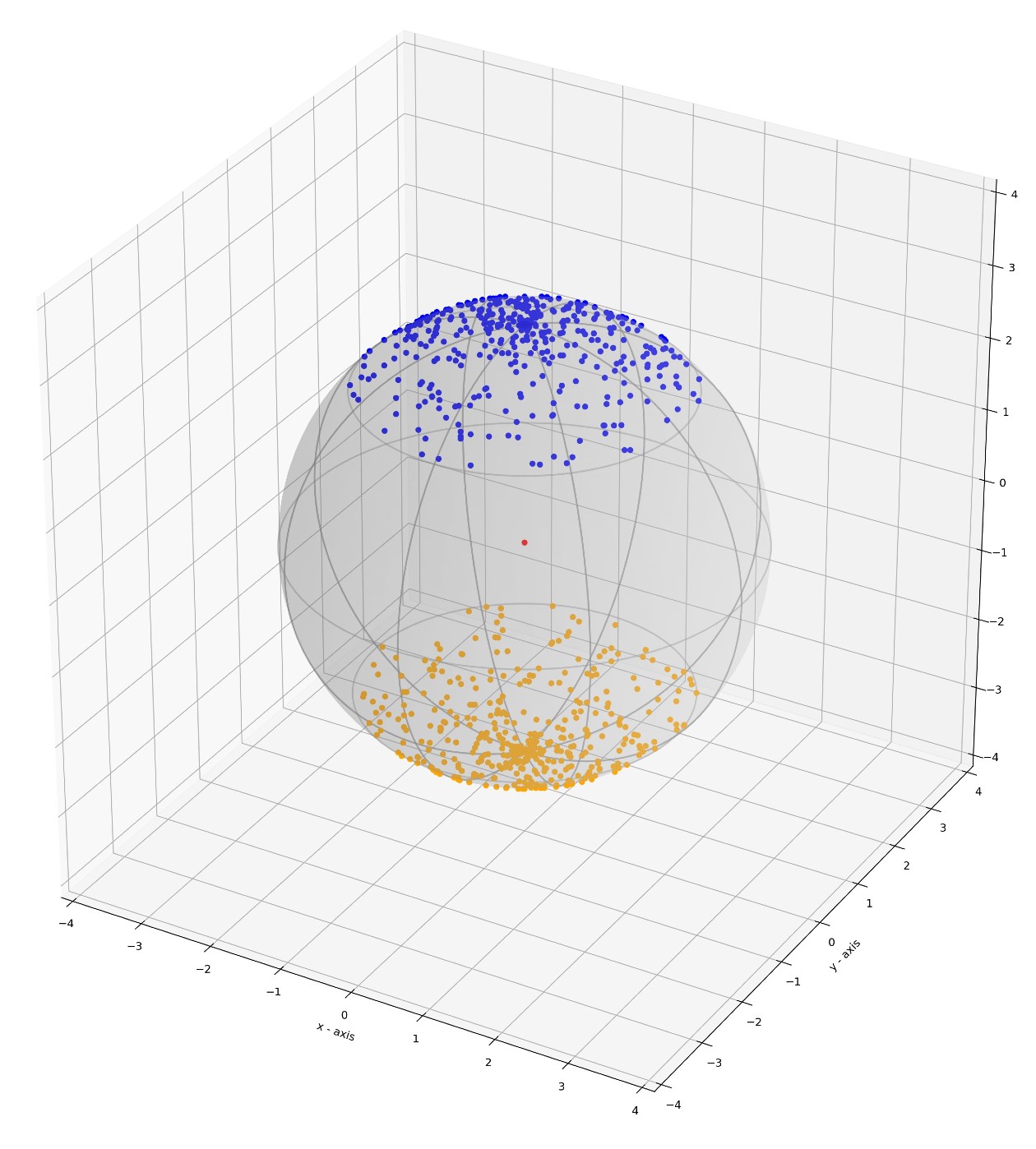
(a)

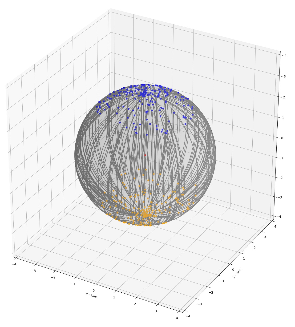
(b)

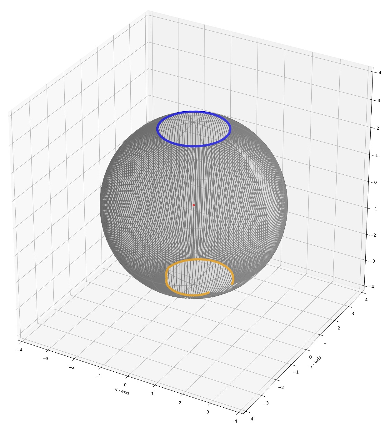
(c)

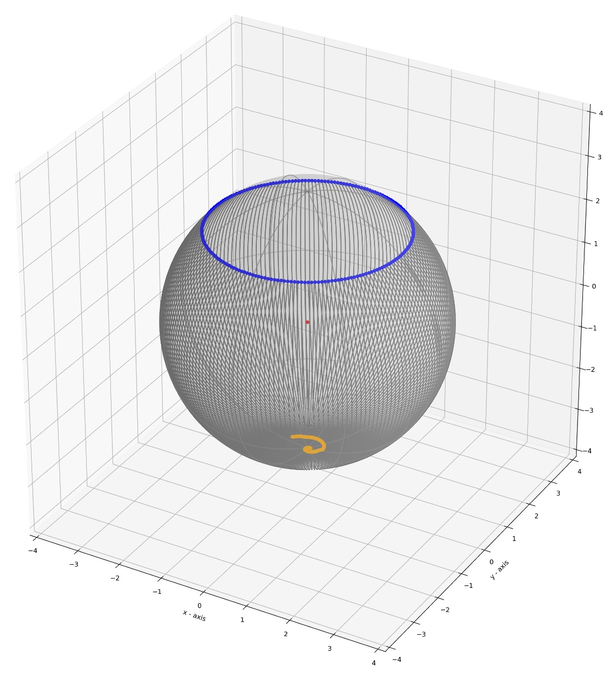
(d)

Figure 11: Monge map from $\rho_{a}$ to $\rho_{b}$ on the sphere: (a) blue samples from $\rho_{a}$ (corresponds to $\hat{\rho}_{a}$) and orange samples from $\rho_{b}$ (corresponds to $\hat{\rho}_{b}$); (b) blue samples from $\rho_{a}$, orange samples are obtained from $\hat{T}_{\sharp}\hat{\rho}_{b}$, grey curves are geodesics connecting each transporting pairs; (c) our computed Monge map maps blue ring ($\phi=\frac{\pi}{8}$) to the orange curve (ground truth is $\phi=\frac{7}{8}\pi$); (d) our computed Monge map maps blue ring ($\phi=\frac{\pi}{4}$) to the orange curve (ground truth is the southpole)

Population transportation

We have described this example in Section 6.3. Here we make further explanation on the map-to-land transform $\tau$, it is defined as follows.

$$\tau(\theta,\phi)=\begin{cases}(\theta,\phi),\quad\textrm{if}~{}(\theta,\phi)\in\textrm{Land};\\ \underset{(\tilde{\theta},\tilde{\phi})\in P}{\textrm{argmin}}\left\{\|(\tilde{\theta},\tilde{\phi})-(\theta,\phi)\|_{2}\right\},\quad\textrm{if}~{}(\theta,\phi)\in\textrm{Sea}.\end{cases}$$

Here we choose $P$ as a finite set consists of $2000$ samples randomly selected from $\rho_{b}^{\textrm{Sph}}$.

We further plot in Figure 12 with sufficiently large amount of source samples and pushforwarded samples. Among the 40000 pushforwarded samples, 7718 are located on the sea, and we apply $\tau$ to map these samples back to a rather close location on land. It is worth mentioning that the map used as the background in our figures has several small regions removed from the actual land. This is due to the lack of data points in the dataset provided in Doxsey-Whitfield et al., (2015).

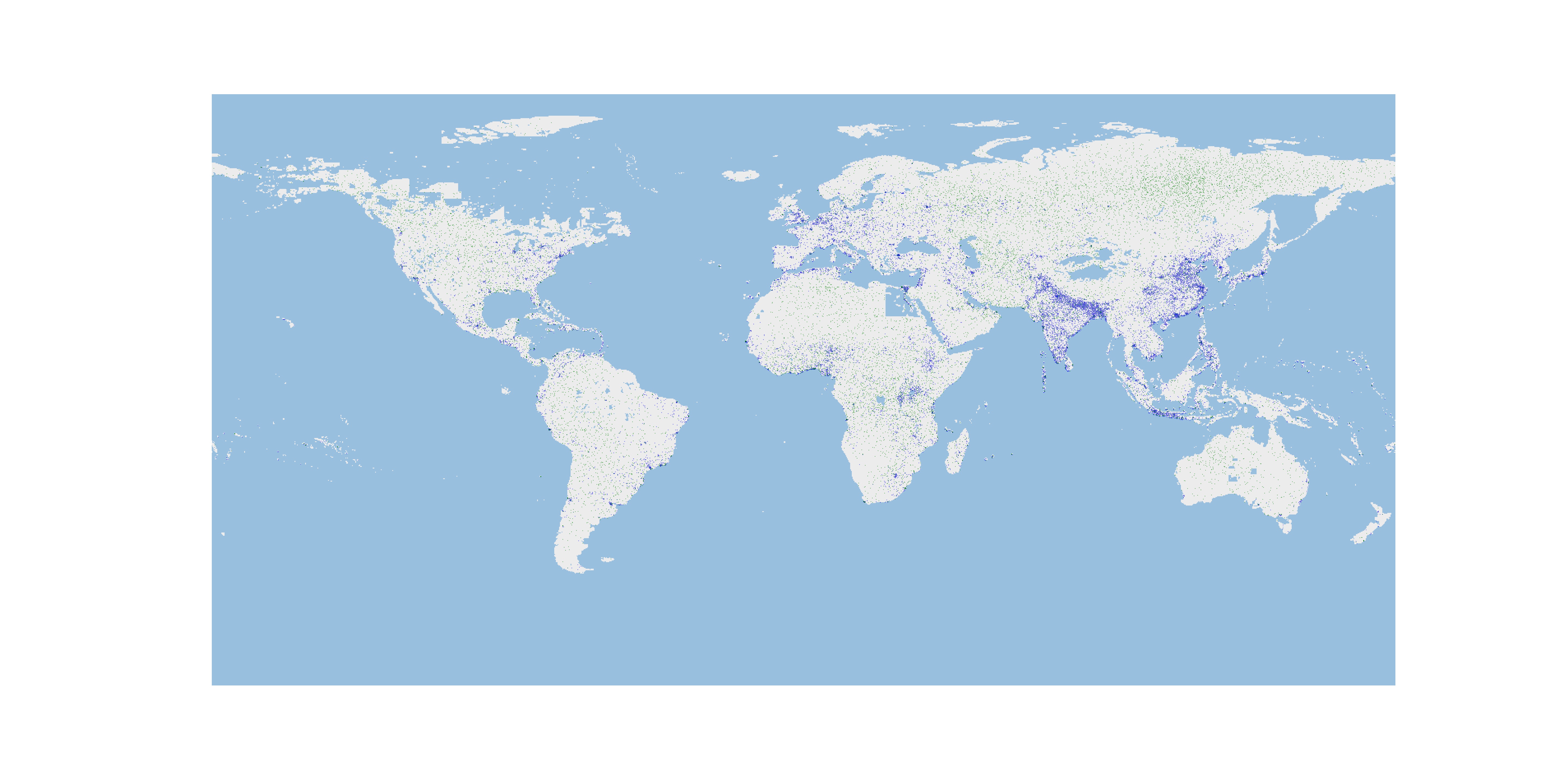
Figure 12: In this figure, we plot $N=40000$ samples $\{\theta_{k},\phi_{k}\}_{k=1}^{N}$ (blue) randomly drawn from $\rho_{a}^{\textrm{Sph}}$, and their pushforwarded samples $\{T_{\theta}(\theta_{k},\phi_{k})\}_{k=1}^{N}$ (green).

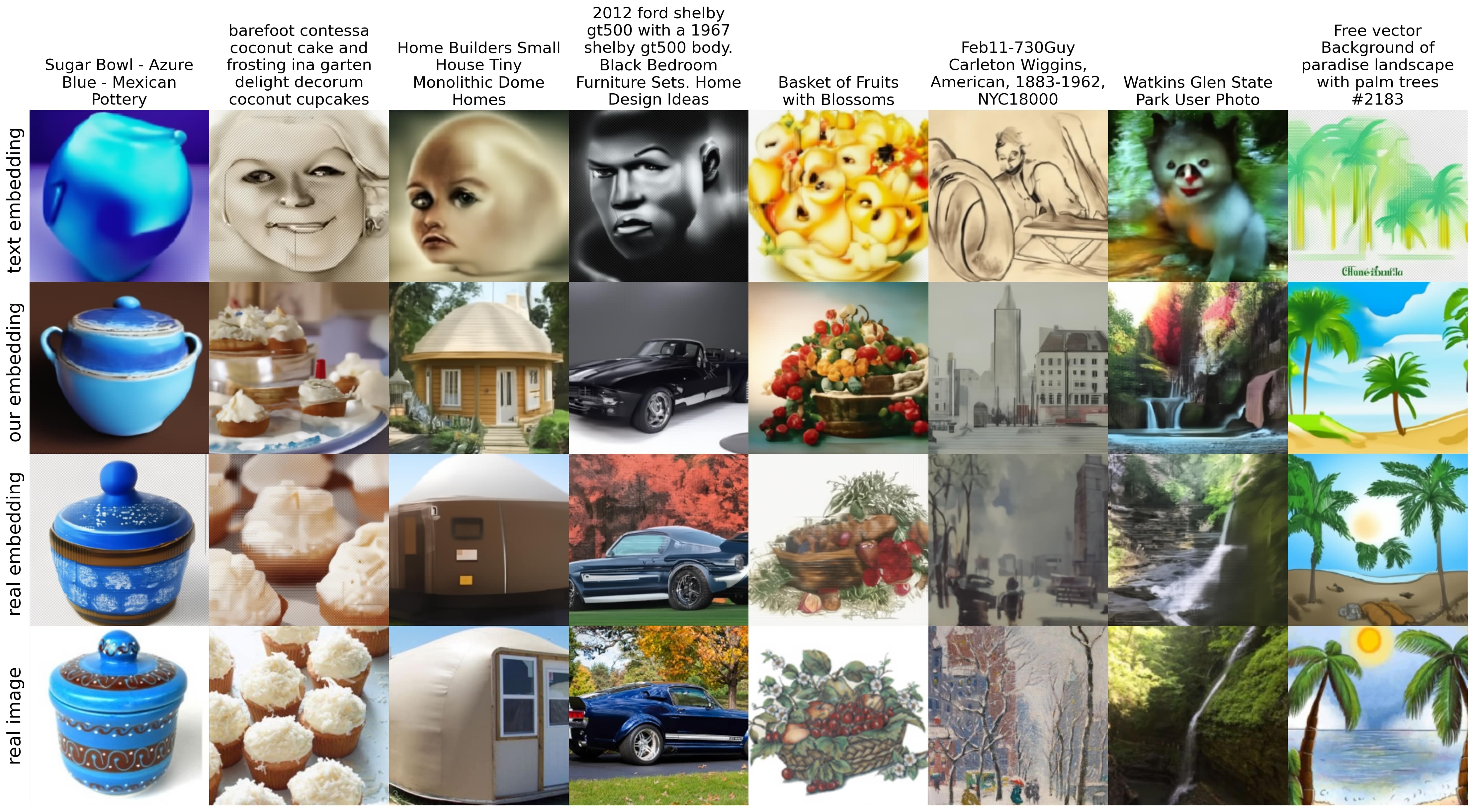
(a) Random image samples on Laion art prompts

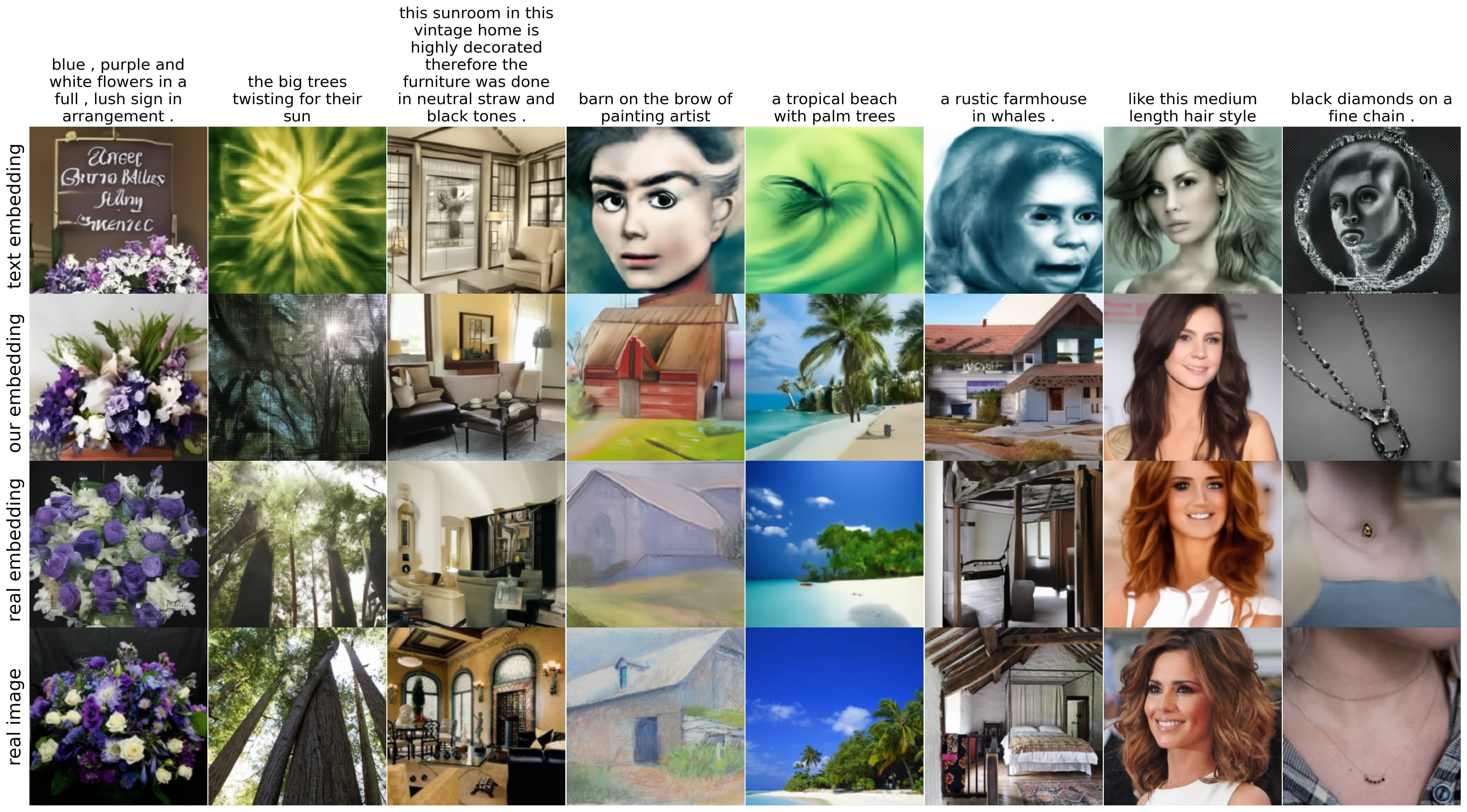
(b) Random image samples on Conceptual Captions 3M prompts

Figure 13: Additional text to image generation results

(a) Degraded and original images

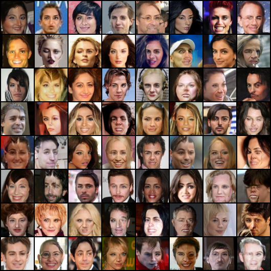
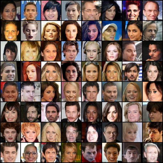
(b) Composite images $G(x)$

(c) Pushforward images $T(x)$

Figure 14: Unpaired image inpainting on test dataset of CelebA $64\times 64$. We take the composite image $G(x)=T(x)\odot M^{C}+x\odot M$ as the output image. Additionally, we provide the pushforward images $T(x)$ to illustrate the regularization effect of transportation cost. In panel (b) and (c), we show the results with $\alpha=10$ in the first row and $\alpha=10000$ in the second row. A small transportation cost would result that pushforward map neglects the connection to the unmasked area, which is illustrated by a more clear mask border in pushforward images.

E.2 Real-world dataset

We show additional text to image generation results by our algorithm in Figure 13, and additional CelebA 64$\times$64 inpainting results in Figure 14. Moreoever, we evaluate our algorithm in the following scenario.

Class-preserving map

We consider the class-preserving map between two labelled datasets. The input distribution $\rho_{a}=\sum_{j=1}^{J}a_{j}\rho^{j}_{a}$ is a mixture of $J$ distinct distributions $\{\rho^{j}_{a}\}_{j=1}^{J}$. Similarly, the target distribution is $\rho_{b}=\sum_{j=1}^{J}a_{j}\rho^{j}_{b}$. Each distribution $\rho_{a}^{j}$ (or $\rho_{b}^{j}$) is associated with a known label/class $j$. We further assume that the support of $\{\rho_{a}^{j}\}$ (or $\rho_{b}^{j}$) are disjoint. We seek a map that solves the problem

$$\min_{\begin{subarray}{c}T_{\sharp}\rho^{j}_{a}=\rho^{j}_{b}\end{subarray}}\int_{\mathbb{R}^{n}}\|x-T(x)\|^{2}\rho_{a}(x)~{}dx,$$ (35)

where the constraint asks the map to preserve the original class. To approximate this map, we replace the constraint by a contrastive penalty. Indeed, this trick transfers (35) to the original Monge problem with a cost

$$c(\{x,y\},\{x^{\prime},y^{\prime}\})=\|x-x^{\prime}\|^{2}+\mathbf{1}(y\neq y^{\prime}),$$

where $y$ and $y^{\prime}$ are the labels corresponding to $x$ and $x^{\prime}$, $\mathbf{1}$ is the indicator function. To better guide the mapping, we involve the label as an input to the mapping $T$ and the potential $f$. Denote $\ell(\cdot):{\mathbb{R}}^{m}\rightarrow{\mathbb{R}}^{J}$ as a pretrained classifier on the target domain $\rho_{b}$. Given a feature from the target domain, $\ell(\cdot)$ will output a probability vector. Then, our full formula reads

$$\sup_{f}\inf_{T} \int\left[c(x,\bar{x})-y^{\top}\bar{y}-f(\bar{x};\bar{y}))\right]d\rho_{a}+\int f(x^{\prime};y^{\prime})d\rho_{b},$$

$$\text{where }\quad\bar{x}=T(x;y),\quad\bar{y}=\ell(T(x;y)).$$

In practice, $y\in{\mathbb{R}}^{J}$ is a one-hot label and it is known because both the source and target datasets are labelled. Our method is different from Asadulaev et al., (2022) because they only solve a map such that $T_{\sharp}\rho^{j}_{a}=\rho^{j}_{b}$, and ignore the transport cost. And their map does not involve the label as input. The closest work to us is the covariate-guided conditional Monge map in Bunne et al., (2022). They use PICNN (Amos et al.,, 2017) to approximate the conditional Monge map and the potential.

We compare our algorithm with Asadulaev et al., (2022) on ^∗NIST (LeCun and Cortes,, 2005; Xiao et al.,, 2017; Clanuwat et al.,, 2018) datasets. The visualization of our mapping is presented in Figure 15. We also calculate FID between the mapped source test dataset and the target test dataset. To quantify how well the map preserves the original class, we use a pretrained SpinalNet classifier (Kabir et al.,, 2022) on the target domain and evaluate the accuracy of the predicted label. If the predicted label of $T(x;y)$ equals to the original label $y$, then the mapping is correct, otherwise wrong. We show the quantitative result in Table 2, where the results of Asadulaev et al., (2022) are from their paper. Our accuracy result is nearly $100\%$ thanks to the contrastive loss guidance. Even though our FID is slightly inferior, we conjecture this can be improved by using a stochastic map (Korotin et al., 2022b, ) as well.

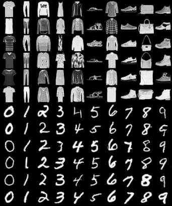
(a) FMNIST $\rightarrow$ MNIST

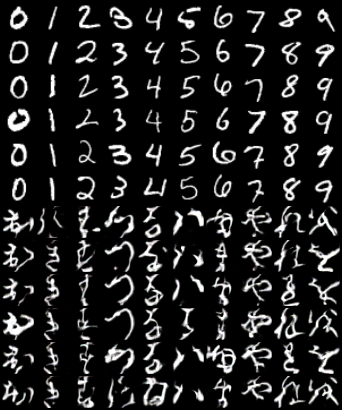
(b) MNIST $\rightarrow$ KMNIST

Figure 15: Class-preserving mapping. The top block is the source images, and the bottom block is the pushforward images. Each column represents a class.

Table 2: Accuracy of the maps and FID of generated samples.

		Asadulaev et al., (2022) deterministic map	Asadulaev et al., (2022) stochastic map	Ours
FID	MNIST $\rightarrow$ KMNSIT	17.26	9.69	18.07
	FMNIST $\rightarrow$ MNIST	7.15	5.26	5.78
Accuracy	MNIST $\rightarrow$ KMNSIT	79.20	61.91	99.59
	FMNIST $\rightarrow$ MNIST	82.97	83.22	99.73

Appendix F Implementation details and hyper-parameters

F.1 Synthetic datasets

Unequal dimensions

The networks $T_{\theta}$ and $f_{\eta}$ each has 5 layers with 10 hidden neurons. The batch size $B=100$. $K_{1}=6,K_{2}=1$. The learning rate is $10^{-3}$. The number of iterations $K=12000.$

Decreasing cost function

In this example, we set $T_{\theta}(x)=x+F_{\theta}(x)$ and optimize over $\theta$. For either $\frac{1}{|x-y|^{2}}$ or $|x-y|^{2}$ case we set both $F_{\theta}$ and the Lagrange multiplier $f_{\eta}$ as six layers fully connected neural networks, with PReLU and Tanh activation functions respectively, each layer has 36 nodes. The training batch size $B=2000$. We set $K=2000$, $K_{1}=8,K_{2}=6$.

On sphere

In this example, we set $T_{\theta}(x)=x+F_{\theta}(x)$ and optimize over $\theta$. We set both $F_{\theta}$ and $f_{\eta}$ as six layers MLP, with PReLU activation functions, each layer has 8 nodes The training batch size is $200$. We set $K=4000$, $K_{1}=8,K_{2}=4$. We choose rather small learning rate in this example to avoid gradient blow up, we set $0.5\times 10^{-5}$ as the learning rate for $\theta$ and $10^{-5}$ as the learning rate for $\eta$.

Population transportation

In this example, we choose both $T_{\theta},f_{\eta}$ as ResNets with depth equals $4$ and hidden dimensions equals $32$; we choose the activation function as PReLU. We apply dropout technique Hinton et al., (2012) with $p=0.24$ to each layer of our networks. We follow the algorithm presented in Algorithm 1 to train the map $T_{\theta}$, We optimize with Adam method with learning rate $5\times 10^{-5}$. $T_{\theta}$ is computed after $200000$ steps of optimization. For the comparison experiment, we tested our example by slightly modifying the codes presented in OT mapping estimation for domain adaptation of POT library Flamary et al., (2021). We train the linear transformation on $2000$ samples from both $\rho_{a}^{\textrm{Sph}}$ and $\rho_{b}^{\textrm{Sph}}$, we choose the hyper parameter $\mu=1,\epsilon=10^{-4}$. We plot the second Figure 8 by applying the map-to-land transform $\tau$ with $2000$ newly selected samples. We also tried the same example with Gaussian kernel, but the results are always unstable for various hyper parameters. Generally speaking, it is very hard to obtain valid results with Gaussian kernel.

F.2 Text to image generation

Dataset details

Laion aesthetic dataset is filtered from a Laion 5B dataset to have the high aesthetic level. Laion art is the subset of Laion aesthetic and contains 8M most aethetic samples. We download the metadata of Laion art according to the instructions of Laion. We then filter only English prompts, and download the images with img2dataset. To speed up the training, we run the CLIP retrieval to convert images to embeddings and use embedding-dataset-reordering to reorder the embeddings into the expected format. By doing these two steps, we save the time of calculating embeddings on the fly. After filtering English prompts, we get the Laion art dataset with 2.2M data.

We download CC-3M following this instruction. We then remove all the images with watermark, which include images downloaded from shutterstock, alamy, gettyimages, and dailymail.co.uk websites. After removing watermark images, the CC-3M only has 0.8M (text, image) pairs left.

For each dataset, we let the source and the target distribution contain 0.3M data respectively, and take the rest of dataset as the test data.

Network structure and hyper-parameters

We use the DALLE$\cdot$2 prior network to represent the map $T$. The potential $f$ is using the same network with an additional pooling layer. We use EMA to stablize the training of the map. The batch size is 225. The number of loop iterations are $K_{1}=10$, $K_{2}=1$. We use the learrning rates $10^{-4}$, Adam (Kingma and Ba,, 2014) optimizer with weight decay coefficient $0.0602$. We train the networks for 110 epochs.

On NVIDIA RTX A6000 (48GB), the training time of each experiment is 21 hours.

F.3 Unpaired inpainting

Recall the composite image is $G(x)=T(x)\odot M^{C}+x\odot M$, where $M$ is the inpainting mask. The loss function is slightly different with the (5). We modify the $f(T(x))$ to be $f(G(x))$ to strengthen the training of $f$

$$\sup_{f}\inf_{T}\int_{\mathbb{R}^{n}}\left[c(x,T(x))-f(G(x))\right]\rho_{a}(x)~{}dx+\int_{\mathbb{R}^{m}}f(y)\rho_{b}(y)~{}dy.$$

In the unpaired inpainting experiments, the images are first cropped at the center with size 140 and then resized to $64\times 64$ or $128\times 128$. We choose learning rate to be $1\cdot 10^{-3}$, Adam optimizer with default beta parameters, $K_{2}=1$. The batch size is 64 for CelebA64 and 16 for CelebA128. The number of inner loop iteration $K_{1}=5$ for CelebA64 and $K_{1}=10$ for CelebA128.

We use exactly the same UNet for the map $T$ and convolutional neural network for $f$ as Rout et al., (2022, Table 9) for CelebA64 and add one additional convolutional block in $f$ network for CelebA128. On NVIDIA RTX A6000 (48GB), the training time of CelebA64 experiment is 10 hours and the time of CelebA128 is 45 hours.

We use the POT implementation of Perrot et al., (2016) as the template and implement the masked MSE loss by ourself. Perrot et al., (2016) provides two options as the transformation map, one is linear and another is the kernel function. We find the kernel function on this example would have generate mode collapse results, so we adopt the linear transformation map. We choose $L_{2}$ regularization coefficient to be $10^{-3}$, and other parameters are the same as default. The result of discrete OT in Figure 6 in the main paper was blue due to an incorrect channel order. We have corrected it in the supplementary material.

F.4 Class preserving mapping

The NIST images are rescaled to size $32\times 32$ and repeated to 3 channels.

We use the conditional UNet to represent map $T$. We add a projection module (Miyato and Koyama,, 2018) on WGAN-QC’s ResNet (Liu et al.,, 2019) to represent potential $f$. We choose learning rate to be $1\cdot 10^{-4}$, Adam optimizer with betas $(0.5,0.999)$. $K_{1}=10,K_{2}=1$. We use EMA to stablize the training of the map. The batch size is 64. In practice, we introduce a coefficient $\lambda$ in the cost $c(\{x,y\},\{x^{\prime},y^{\prime}\})=\|x-x^{\prime}\|^{2}+\lambda\mathbf{1}(y\neq y^{\prime})$ and set $\lambda=0.5$.

References

- Afriat, (1971) Afriat, S. (1971). Theory of maxima and the method of lagrange. SIAM Journal on Applied Mathematics, 20(3):343–357.
- Altschuler et al., (2017) Altschuler, J., Niles-Weed, J., and Rigollet, P. (2017). Near-linear time approximation algorithms for optimal transport via sinkhorn iteration. Advances in neural information processing systems, pages 1964–1974.
- Alvarez-Melis and Fusi, (2020) Alvarez-Melis, D. and Fusi, N. (2020). Geometric dataset distances via optimal transport. Advances in Neural Information Processing Systems, 33:21428–21439.
- Alvarez-Melis et al., (2021) Alvarez-Melis, D., Schiff, Y., and Mroueh, Y. (2021). Optimizing functionals on the space of probabilities with input convex neural networks. arXiv preprint arXiv:2106.00774.
- Amos et al., (2022) Amos, B., Cohen, S., Luise, G., and Redko, I. (2022). Meta optimal transport.
- Amos et al., (2017) Amos, B., Xu, L., and Kolter, J. (2017). Input convex neural networks. In International Conference on Machine Learning, pages 146–155.
- Arjovsky et al., (2017) Arjovsky, M., Chintala, S., and Bottou, L. (2017). Wasserstein gan. In arXiv preprint arXiv:1701.07875.
- Asadulaev et al., (2022) Asadulaev, A., Korotin, A., Egiazarian, V., and Burnaev, E. (2022). Neural optimal transport with general cost functionals. arXiv preprint arXiv:2205.15403.
- Bunne et al., (2022) Bunne, C., Krause, A., and Cuturi, M. (2022). Supervised training of conditional monge maps. arXiv preprint arXiv:2206.14262.
- Bunne et al., (2021) Bunne, C., Meng-Papaxanthos, L., Krause, A., and Cuturi, M. (2021). Jkonet: Proximal optimal transport modeling of population dynamics. arXiv preprint arXiv:2106.06345.
- Clanuwat et al., (2018) Clanuwat, T., Bober-Irizar, M., Kitamoto, A., Lamb, A., Yamamoto, K., and Ha, D. (2018). Deep learning for classical japanese literature. arXiv preprint arXiv:1812.01718.
- Courty et al., (2017) Courty, N., Flamary, R., Habrard, A., and Rakotomamonjy, A. (2017). Joint distribution optimal transportation for domain adaptation. Advances in Neural Information Processing Systems, 30.
- Courty et al., (2016) Courty, N., Flamary, R., Tuia, D., and Rakotomamonjy, A. (2016). Optimal transport for domain adaptation. IEEE transactions on pattern analysis and machine intelligence, 39(9):1853–1865.
- Cuturi, (2013) Cuturi, M. (2013). Sinkhorn distances: Lightspeed computation of optimal transport. In Neural Information Processing Systems.
- Doxsey-Whitfield et al., (2015) Doxsey-Whitfield, E., MacManus, K., Adamo, S. B., Pistolesi, L., Squires, J., Borkovska, O., and Baptista, S. R. (2015). Taking advantage of the improved availability of census data: A first look at the gridded population of the world, version 4. Papers in Applied Geography, 1(3):226–234.
- (16) Fan, J., Haasler, I., Karlsson, J., and Chen, Y. (2022a). On the complexity of the optimal transport problem with graph-structured cost. In International Conference on Artificial Intelligence and Statistics, pages 9147–9165. PMLR.
- Fan et al., (2020) Fan, J., Taghvaei, A., and Chen, Y. (2020). Scalable computations of wasserstein barycenter via input convex neural networks. arXiv preprint arXiv:2007.04462.
- (18) Fan, J., Zhang, Q., Taghvaei, A., and Chen, Y. (2022b). Variational Wasserstein gradient flow. In Chaudhuri, K., Jegelka, S., Song, L., Szepesvari, C., Niu, G., and Sabato, S., editors, Proceedings of the 39th International Conference on Machine Learning, volume 162 of Proceedings of Machine Learning Research, pages 6185–6215. PMLR.
- Feydy et al., (2020) Feydy, J., Glaunès, A., Charlier, B., and Bronstein, M. (2020). Fast geometric learning with symbolic matrices. Advances in Neural Information Processing Systems, 33:14448–14462.
- Flamary et al., (2021) Flamary, R., Courty, N., Gramfort, A., Alaya, M. Z., Boisbunon, A., Chambon, S., Chapel, L., Corenflos, A., Fatras, K., Fournier, N., Gautheron, L., Gayraud, N. T., Janati, H., Rakotomamonjy, A., Redko, I., Rolet, A., Schutz, A., Seguy, V., Sutherland, D. J., Tavenard, R., Tong, A., and Vayer, T. (2021). Pot: Python optimal transport. Journal of Machine Learning Research, 22(78):1–8.
- Gazdieva et al., (2022) Gazdieva, M., Rout, L., Korotin, A., Filippov, A., and Burnaev, E. (2022). Unpaired image super-resolution with optimal transport maps. arXiv preprint arXiv:2202.01116.
- Genevay et al., (2016) Genevay, A., Cuturi, M., Peyré, G., and Bach, F. (2016). Stochastic optimization for large-scale optimal transport. In Advances in neural information processing systems, pages 3440–3448.
- Genevay et al., (2018) Genevay, A., Peyré, G., and Cuturi, M. (2018). Learning generative models with sinkhorn divergences. International Conference on Artificial Intelligence and Statistics, pages 1608–1617.
- Gulrajani et al., (2017) Gulrajani, I., Ahmed, F., Arjovsky, M., Dumoulin, V., and Courville, A. C. (2017). Improved training of wasserstein gans. Advances in neural information processing systems, 30.
- Haasler et al., (2020) Haasler, I., Singh, R., Zhang, Q., Karlsson, J., and Chen, Y. (2020). Multi-marginal optimal transport and probabilistic graphical models. In arXiv preprint arXiv:2006.14113.
- Heusel et al., (2017) Heusel, M., Ramsauer, H., Unterthiner, T., Nessler, B., and Hochreiter, S. (2017). Gans trained by a two time-scale update rule converge to a local nash equilibrium. Advances in neural information processing systems, 30.
- Hinton et al., (2012) Hinton, G. E., Srivastava, N., Krizhevsky, A., Sutskever, I., and Salakhutdinov, R. R. (2012). Improving neural networks by preventing co-adaptation of feature detectors.
- Hütter and Rigollet, (2020) Hütter, J.-C. and Rigollet, P. (2020). Minimax estimation of smooth optimal transport maps.
- Inoue et al., (2020) Inoue, D., Ito, Y., and Yoshida, H. (2020). Optimal transport-based coverage control for swarm robot systems: Generalization of the voronoi tessellation-based method. IEEE Control Systems Letters, 5(4):1483–1488.
- Kabir et al., (2022) Kabir, H. D., Abdar, M., Khosravi, A., Jalali, S. M. J., Atiya, A. F., Nahavandi, S., and Srinivasan, D. (2022). Spinalnet: Deep neural network with gradual input. IEEE Transactions on Artificial Intelligence.
- Kingma and Ba, (2014) Kingma, D. P. and Ba, J. (2014). Adam: A method for stochastic optimization.
- (32) Korotin, A., Egiazarian, V., Asadulaev, A., Safin, A., and Burnaev, E. (2021a). Wasserstein-2 generative networks. In International Conference on Learning Representations.
- (33) Korotin, A., Egiazarian, V., Li, L., and Burnaev, E. (2022a). Wasserstein iterative networks for barycenter estimation. arXiv preprint arXiv:2201.12245.
- (34) Korotin, A., Li, L., Genevay, A., Solomon, J., Filippov, A., and Burnaev, E. (2021b). Do neural optimal transport solvers work? a continuous wasserstein-2 benchmark. In arXiv preprint arXiv:2106.01954.
- (35) Korotin, A., Li, L., Solomon, J., and Burnaev, E. (2021c). Continuous wasserstein-2 barycenter estimation without minimax optimization. arXiv preprint arXiv:2102.01752.
- (36) Korotin, A., Selikhanovych, D., and Burnaev, E. (2022b). Neural optimal transport. arXiv preprint arXiv:2201.12220.
- Krishnan and Martínez, (2018) Krishnan, V. and Martínez, S. (2018). Distributed optimal transport for the deployment of swarms. IEEE Conference on Decision and Control (CDC), pages 4583–4588.
- LeCun and Cortes, (2005) LeCun, Y. and Cortes, C. (2005). The mnist database of handwritten digits.
- Li et al., (2019) Li, R., Ye, X., Zhou, H., and Zha, H. (2019). Learning to match via inverse optimal transport. In J. Mach. Learn. Res., pages 20, pp.80–1.
- Liu et al., (2019) Liu, H., Gu, X., and Samaras, D. (2019). Wasserstein gan with quadratic transport cost. In Proceedings of the IEEE/CVF international conference on computer vision, pages 4832–4841.
- Liu et al., (2015) Liu, Z., Luo, P., Wang, X., and Tang, X. (2015). Deep learning face attributes in the wild. In Proceedings of the IEEE international conference on computer vision, pages 3730–3738.
- Ma et al., (2020) Ma, S., Liu, S., Zha, H., and Zhou, H. (2020). Learning stochastic behaviour of aggregate data. In arXiv preprint arXiv:2002.03513.
- Makkuva et al., (2020) Makkuva, A.and Taghvaei, A., Oh, S., and Lee, J. (2020). Optimal transport mapping via input convex neural networks. In International Conference on Machine Learning, pages 6672–6681.
- Meng et al., (2019) Meng, C., Ke, Y., Zhang, J., Zhang, M., Zhong, W., and Ma, P. (2019). Large-scale optimal transport map estimation using projection pursuit. Advances in Neural Information Processing Systems, 32.
- Miyato and Koyama, (2018) Miyato, T. and Koyama, M. (2018). cgans with projection discriminator. arXiv preprint arXiv:1802.05637.
- Mokrov et al., (2021) Mokrov, P., Korotin, A., Li, L., Genevay, A., Solomon, J., and Burnaev, E. (2021). Large-scale wasserstein gradient flows. In Thirty-Fifth Conference on Neural Information Processing Systems.
- Nash, (2000) Nash, J. C. (2000). The (dantzig) simplex method for linear programming. Computing in Science & Engineering, 2(1):29–31.
- Nhan Dam et al., (2019) Nhan Dam, Q. H., Le, T., Nguyen, T. D., Bui, H., and Phung, D. (2019). Threeplayer wasserstein gan via amortised duality. In Proc. of the 28th Int. Joint Conf. on Artificial Intelligence (IJCAI), pages 1–11.
- Obukhov et al., (2020) Obukhov, A., Seitzer, M., Wu, P.-W., Zhydenko, S., Kyl, J., and Lin, E. Y.-J. (2020). High-fidelity performance metrics for generative models in pytorch. Version: 0.3.0, DOI: 10.5281/zenodo.4957738.
- Perrot et al., (2016) Perrot, M., Courty, N., Flamary, R., and Habrard, A. (2016). Mapping estimation for discrete optimal transport. Advances in Neural Information Processing Systems, 29.
- Pooladian and Niles-Weed, (2021) Pooladian, A.-A. and Niles-Weed, J. (2021). Entropic estimation of optimal transport maps. arXiv preprint arXiv:2109.12004.
- Radford et al., (2021) Radford, A., Kim, J. W., Hallacy, C., Ramesh, A., Goh, G., Agarwal, S., Sastry, G., Askell, A., Mishkin, P., Clark, J., et al. (2021). Learning transferable visual models from natural language supervision. In International Conference on Machine Learning, pages 8748–8763. PMLR.
- Ramesh et al., (2022) Ramesh, A., Dhariwal, P., Nichol, A., Chu, C., and Chen, M. (2022). Hierarchical text-conditional image generation with clip latents. arXiv preprint arXiv:2204.06125.
- Ramesh et al., (2021) Ramesh, A., Pavlov, M., Goh, G., Gray, S., Voss, C., Radford, A., Chen, M., and Sutskever, I. (2021). Zero-shot text-to-image generation. In International Conference on Machine Learning, pages 8821–8831. PMLR.
- Rout et al., (2022) Rout, L., Korotin, A., and Burnaev, E. (2022). Generative modeling with optimal transport maps. In International Conference on Learning Representations.
- Saharia et al., (2022) Saharia, C., Chan, W., Saxena, S., Li, L., Whang, J., Denton, E., Ghasemipour, S. K. S., Ayan, B. K., Mahdavi, S. S., Lopes, R. G., et al. (2022). Photorealistic text-to-image diffusion models with deep language understanding. arXiv preprint arXiv:2205.11487.
- Seguy et al., (2017) Seguy, V., Damodaran, B., Flamary, R., Courty, N., R., A., and Blondel, M. (2017). Large-scale optimal transport and mapping estimation. arXiv preprint arXiv:1711.02283.
- Villani, (2003) Villani, C. (2003). Topics in optimal transportation. Number 58. American Mathematical Soc.
- Villani, (2008) Villani, C. (2008). Optimal transport: old and new, volume 338. Springer Science & Business Media.
- Xiao et al., (2017) Xiao, H., Rasul, K., and Vollgraf, R. (2017). Fashion-mnist: a novel image dataset for benchmarking machine learning algorithms. arXiv preprint arXiv:1708.07747.
- Xie et al., (2020) Xie, Y., Wang, X., Wang, R., and Zha, H. (2020). A fast proximal point method for computing exact wasserstein distance. In Uncertainty in Artificial Intelligence, pages 433–453.
- Yang and Uhler, (2018) Yang, K. D. and Uhler, C. (2018). Scalable unbalanced optimal transport using generative adversarial networks. arXiv preprint arXiv:1810.11447.
- Zeng et al., (2021) Zeng, Y., Lin, Z., Lu, H., and Patel, V. M. (2021). Cr-fill: Generative image inpainting with auxiliary contextual reconstruction. In Proceedings of the IEEE/CVF International Conference on Computer Vision, pages 14164–14173.