Deep Medial Fields

Abstract.

Implicit representations of geometry, such as occupancy fields or signed distance fields (SDF), have recently re-gained popularity in encoding 3D solid shape in a functional form. In this work, we introduce medial fields: a field function derived from the medial axis transform (MAT) that makes available information about the underlying 3D geometry that is immediately useful for a number of downstream tasks. In particular, the medial field encodes the local thickness of a 3D shape, and enables O(1) projection of a query point onto the medial axis. To construct the medial field we require nothing but the SDF of the shape itself, thus allowing its straightforward incorporation in any application that relies on signed distance fields. Working in unison with the O(1) surface projection supported by the SDF, the medial field opens the door for an entirely new set of efficient, shape-aware operations on implicit representations. We present three such applications, including a modification to sphere tracing that renders implicit representations with better convergence properties, a fast construction method for memory-efficient rigid-body collision proxies, and an efficient approximation of ambient occlusion that remains stable with respect to viewpoint variations.

grid \begin{overpic}[width=143.09538pt]{fig/lucy_teaser_mf_right.png} \put(43.0,63.0){SDF} \put(38.0,59.0){{\scriptsize($\approx$6 it/pix)}} \put(54.5,63.0){DMF} \put(54.5,59.0){{\scriptsize($\approx$4 it/pix)}} \put(23.0,-5.0){rendering implicit functions} \end{overpic} \begin{overpic}[width=143.09538pt,trim=50.18748pt 60.22499pt 50.18748pt 0.0pt,clip]{fig/rocker-arm_teaser.png} \put(13.0,-5.0){generation of collision proxies} \end{overpic} \begin{overpic}[width=143.09538pt]{fig/mecha_teaser.png} \put(33.0,63.0){No AO} \put(52.0,63.0){MFAO} \put(20.0,-5.0){efficient ambient occlusion} \end{overpic}

Figure 1. Deep medial field implicitly encode information related to the medial axis in a neural field function. Such a function can be used to accelerate iterative ray tracing of implicits (left), quickly compute physics acceleration proxies (middle), or implement a new form of ambient occlusion (right).

1. Introduction

Neural implicit representations of 3D geometry and appearance have recently emerged as an attractive alternative to conventional discrete representations such as polygonal meshes or grids. For example, Mescheder et al. (2019) and Park et al. (2019) store geometry of a 3D object as occupancy and signed distance field, while Sitzmann et al. (2019) and Mildenhall et al. (2020) additionally infer appearance via differentiable rendering. These new neural representations enable spatially adaptive and high-resolution shape representations of 3D signals, while allowing the learning of priors over shape (Chen and Zhang, 2019) and appearance (Oechsle et al., 2019; Sitzmann et al., 2019). In this work, we investigate a novel representation of 3D geometric information that gives O(1) access to quantities immediately useful to a variety of downstream tasks.

Medial field

Specifically, we introduce the analytical concept of medial fields. The medial field, as in the case of occupancy and SDF, is a scalar function defined over $\mathbb{R}^{d}$. While signed distance functions retrieve the radius of an empty sphere centered at $x$ that is tangent to the surface of an object, medial fields query the local thickness at the query point $x$. Local thickness expresses the size of a sphere that is related to the one retrieved by the SDF: it is tangent to the object surface at the same location, it fully contains the SDF sphere, and it is the largest empty sphere satisfying these properties. However, assuming we can easily and efficiently retrieve it with O(1) complexity, “What applications could it enable?”

Applications

In this paper we explore a (likely incomplete) portfolio of applications for medial fields. First and foremost, we look at the classical problem of rendering implicit functions, and realize that the popular “sphere tracing” algorithm proposed by Hart (1996) relies on iteratively querying empty spheres provided by the signed distance function. Conversely, by exploiting medial fields, we can compute spheres that are larger, resulting in fewer, larger steps, and hence an overall improved convergence rate; see Figure 1 (left) We then consider real-time physics simulation, for which the efficient computation of collision proxies is of central importance, and that typically involve classical algorithms executed on polygonal meshes (Ericson, 2004). We instead propose a solution that extracts a volumetric approximation as a collection of spheres, where the locally largest empty spheres queried by the medial sphere result in an efficient coverage of space without using an excessive number of proxies; see Figure 1 (middle). Finally, we employ local thickness as a way to efficiently identify deep creases in the surface of objects where light is unlikely to reach, hence providing a method to approximate ambient occlusion shading effects within the realm of implicit shape representations; see Figure 1 (right) While these applications showcase the versatility of medial fields, we must ask the question: “How can we compute (and store) medial fields?”

Computation

In computational geometry, the concept of local thickness is formalized by the Medial Axis Transform (Blum et al., 1967), a dual representation of solid geometry from which we derive the nomenclature “medial field”. Medial axis computation has been studied extensively in computer science, but the design of algorithms as effective as for other types of transforms (e.g. the Fourier Transform) has been elusive; the problem is particularly dire in $\mathbb{R}^{3}$, where the computation of the medial surfaces from polygonal meshes essentially remains an open challenge (Tagliasacchi et al., 2016). We overcome these issues by expressing the problem of medial field computation as a continuous constrained satisfaction problem, which we approach by stochastic optimization, and that only requires querying the signed distance field. Further, rather than relying on discrete grids to store medial fields, whose memory requirements are excessive at high resolutions, we compactly store the medial field function within the parameters of a neural network.

To summarize, in this paper we introduce:

• “medial fields” as a way to augment signed distance fields with meta-information capturing local thickness of both a shape and its complement space;

• a portfolio of applications that leverage medial fields for efficient rendering, generation of collision proxies, and deferred rendering;

• medial field computation as a constraint optimization problem that stores the field function within the parameters of a deep neural network for compact storage, and O(1) query access time.

2. Related works

Our technique is tightly related to implicit neural representations (Section 2.1), as well as their efficient rendering (Section 2.2). Medial fields are also heavily inspired by medial axis techniques, which we also briefly review (Section 2.3).

2.1. Neural implicit representations

Inspired by classic work on implicit representation of geometry (Bloomenthal et al., 1997; Blinn, 1982), a recent class of models has leveraged fully connected neural networks as continuous, memory-efficient representations of 3D scene geometry, by parameterizing either a distance field (Park et al., 2019; Michalkiewicz et al., 2019; Atzmon and Lipman, 2020; Gropp et al., 2020; Sitzmann et al., 2019; Jiang et al., 2020; Peng et al., 2020; Chibane et al., 2020) or the occupancy function (Mescheder et al., 2019; Chen and Zhang, 2019) of the 3D geometry. Learning priors over spaces of neural implicit representations enables reconstruction from partial observations (Park et al., 2019; Mescheder et al., 2019; Chen and Zhang, 2019; Sitzmann et al., 2020a). To learn distance fields when ground-truth distance values are unavailable, we may solve the Eikonal equation (Atzmon and Lipman, 2020; Sitzmann et al., 2020b; Gropp et al., 2020), or leverage the property that points may be projected onto the surface by stepping in the direction of the gradient (Ma et al., 2020). One may leverage hybrid implicit-explicit representations, by locally conditioning a neural implicit representation on features stored in a discrete data structure such as a voxel grids (Jiang et al., 2020; Peng et al., 2020; Chabra et al., 2020), octrees (Takikawa et al., 2021), or local Gaussians (Genova et al., 2019). However, such hybrid implicit-explicit representations lose the compactness of monolithic representations, complicating the learning of shape spaces. In this work, we propose to parameterize 3D shape via the medial field, which parameterizes the local thickness of a 3D shape, and gives O(1) access to a number of quantities immediately useful for downstream tasks.

2.2. Rendering implicits

Rendering of implicit shape representations relies on the discovery of the first level set that a camera ray intersects. For distance fields, sphere tracing (Hart, 1996) enables fast root-finding. This algorithm known pathological cases, which have been addressed with heuristics (Bálint and Valasek, 2018; Korndörfer et al., 2014), as well as coarse-to-fine schemes (Liu et al., 2020). Ours is complementary to these approaches, and we focus our comparison on the core algorithm. Additionally, sphere tracing can be generalized to the rendering of deformed implicit representations (Seyb et al., 2019).

For neural implicit shape representations, differentiable renderers have been proposed to learn implicit representations of geometry given only 2D observations of 3D scenes (Sitzmann et al., 2019; Liu et al., 2020; Niemeyer et al., 2020; Yariv et al., 2020). Alternatively, one may parameterize density and radiance of a 3D scene, enabling volumetric rendering (Mildenhall et al., 2020), or combine volumetric and ray-marching based approaches (Oechsle et al., 2021). As rendering of neural implicit representations requires hundreds of evaluations of the distance field per ray, hybrid explicit-implicit representations have been proposed to provide significant speedups (Takikawa et al., 2021). As we will demonstrate, the proposed Deep Medial Fields allow fast rendering as they require significantly fewer network evaluations per ray, without relying on a hybrid implicit-explicit representation.

2.3. Medial axis transform (MAT)

The medial axis transform provides a dual representation of solid geometry as a collection of spheres. Computing the medial axis is a challenging problem, due to both the instability of this representation with respect to noise (Rebain et al., 2019, Fig.3), and the lack of techniques to compute the medial surfaces given a polygonal mesh (Tagliasacchi et al., 2016). Nonetheless, spherical representations “inspired” by the MAT have found widespread use in applications, including shape approximation for static (Thiery et al., 2013) and dynamic (Thiery et al., 2016) geometry, efficient closest point computation (Tkach et al., 2016), and volumetric physics simulation (Angles et al., 2019). There has been work on constructing the MAT with neural networks (Hu et al., 2019), but to the best of our knowledge, ours is the first work to encode medial information in an implicit neural representation.

3. Method

We start by reviewing the basics of implicit and medial representations (Section 3.1), and then introduce the analytical concept of medial fields (Section 3.2). We then propose a variational formulation of medial fields which allows us to formalize it without requiring us to explicitly compute the medial axis (Section 3.3), as well as a way of implementing this approach with neural networks (Section 3.4).

3.1. Background

Let us consider a (solid) shape $\mathcal{O}$ in $d$-dimensional space as partitioning all points $x\in\mathbb{R}^{d}$ as belonging to either its interior $\mathcal{O}^{-}$, exterior $\mathcal{O}^{+}$, or (boundary) surface $\partial\mathcal{O}$. The signed and unsigned distance fields (respectively SDF and UDF) implicitly represent a shape as:

(1) $$\Phi(x)=\begin{cases}+\mathbf{d}(x)&x\in\mathcal{O}^{+}\\ -\mathbf{d}(x)&x\in\mathcal{O}^{-}\\ 0&x\in\partial\mathcal{O}\end{cases}\;,\quad\mathbf{d}(x)=\min_{y\in\partial\mathcal{O}}||x-y||\;,$$

where the term implicit refers to the fact that the shape boundary is indirectly defined as the zero-crossing of the field.

     

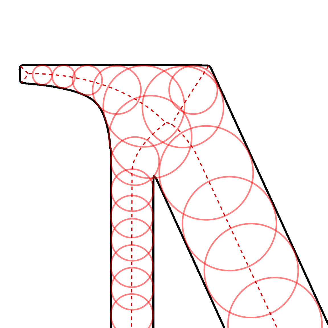
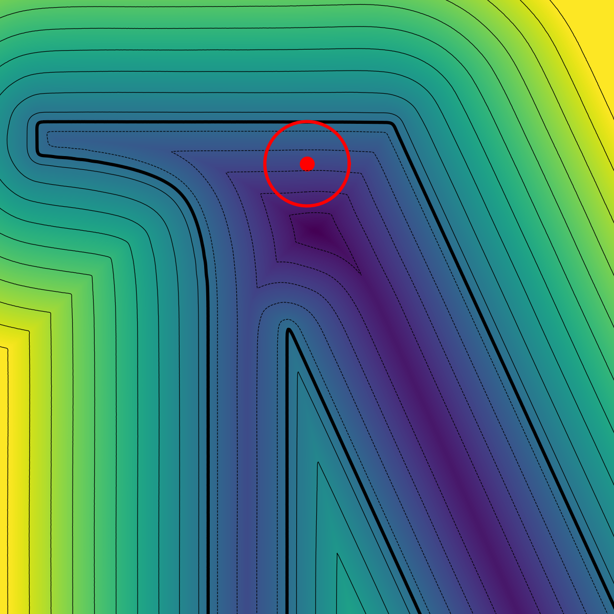
Figure 2. Medial axis and the SDF – (left) Interpretation of the medial axis as the set of maximally inscribed sphere. (right) The signed distance function $\Phi(x)$ of the shape, and a tangent sphere.

The medial axis

The Medial Axis Transform (MAT) of a shape is the set of “maximally inscribed spheres”. The medial axis $\mathcal{M}$ can then be defined as the set of all centers of these spheres:

(2) $$\mathcal{M}=\{x\in\mathbb{R}^{d}:\,\forall\delta\in\mathbb{R}^{d}\setminus\mathbf{0},\mathbf{d}(x)+||\delta||>\mathbf{d}(x+\delta)\}\;.$$

As illustrated in Figure 2, note that $\mathbf{d}(x)$ is equal to the radius of an empty sphere centered at $x$ and tangent to $\partial\mathcal{O}$. Any tangent sphere that can not be grown to a tangent sphere with a $||\delta||$-larger radius by moving the center with some offset $\delta$ is “maximally inscribed”, and therefore a medial sphere. While there exist multiple ways to define the medial axis (Tagliasacchi et al., 2016), we choose this definition as it will allow us to formulate the medial axis in terms of a field function: the “medial field”.

     

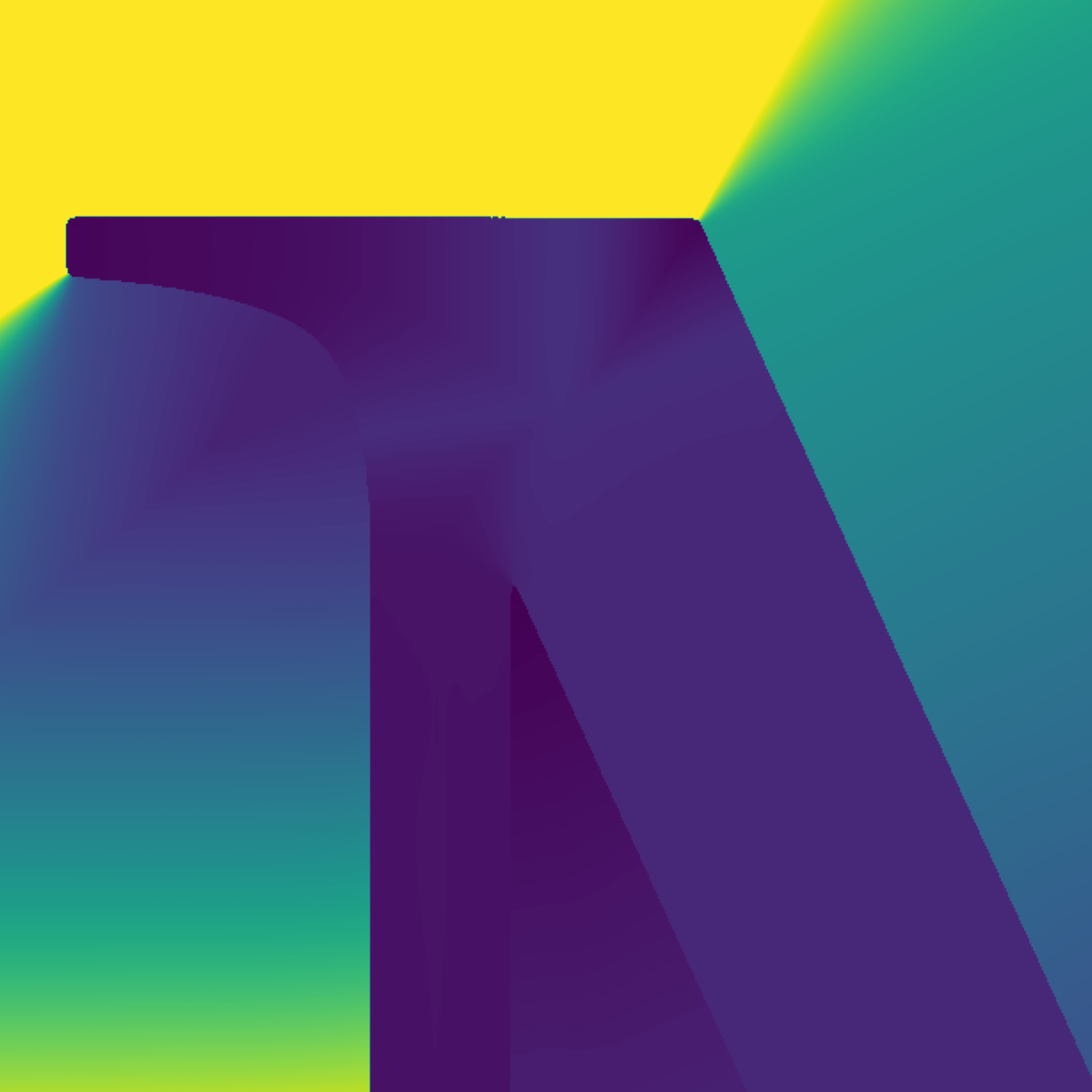
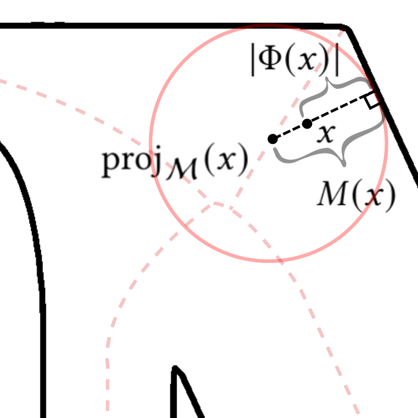
Figure 3. Medial field – (left) Visualization of the scalar medial field; (right) The notation we use to define the medial field; note that for $x\in\mathcal{M}$ the medial field and the unsigned distance function satisfy $M(x)=|\Phi(x)|$.

3.2. Medial field

For a point $x\in\mathcal{O}^{-}$, we informally define the medial field as the “local thickness” of the shape at $x$, and equivalently for the shape’s complement space when $x\in\mathcal{O}^{+}$; see Figure 3 (left). To formalize this construct, let us start by noting that $\Phi(x)$ allows us to project a point $x$ onto the closest point of the shape surface $\partial\mathcal{O}$ as:

(3) $$\mathrm{proj}_{\mathcal{O}}(x)=x-\nabla\Phi(x)\Phi(x)\;.$$

Both $x$ and $\mathrm{proj}_{\mathcal{O}}(x)$ lie on a line segment $\mathbf{s}(x)$, known as the “medial spoke” (Siddiqi and Pizer, 2008), which begins at $\mathrm{proj}_{\mathcal{O}}(x)$ and ends at a point on the medial axis; see Figure 3 (right). We call this point $\mathrm{proj}_{\mathcal{M}}(x)$, and use it to define the medial field as the scalar function:

(4) $$M(x)=|\Phi(\mathrm{proj}_{\mathcal{M}}(x))|\;.$$

In other words, the medial field $M(x)$ is the radius of the medial sphere centered at $\mathrm{proj}_{\mathcal{M}}(x)$. Equivalently, the medial field is the length of the medial spoke $\mathbf{s}(x)$. $M(x)$ is well defined everywhere except at $x\in\partial\mathcal{O}$ where we could have a value discontinuity – the medial field for interior/exterior might not match. While above we employ $\mathrm{proj}_{\mathcal{M}}$ to define the medial field, the opposite is also possible:

(5) $$\mathrm{proj}_{\mathcal{M}}(x)=x+\nabla|\Phi(x)|(M(x)-|\Phi(x)|)\;,$$

but note that $\mathrm{proj}_{\mathcal{M}}(x)$ is not the closest-point projection of $x$ onto $\mathcal{M}$, but rather the intersection of the medial spoke with $\mathcal{M}$.

3.3. Variational medial fields

To use medial fields in an application, one must first compute it. With the definitions above, given $\Phi(x)$ and $\nabla\Phi(x)$, the medial field could be computed explicitly by querying the medial radius at the intersection of the medial spoke and the medial axis. Unfortunately, computing the medial axis, especially in $\mathbb{R}^{3}$, is a challenging and open problem (Tagliasacchi et al., 2016). Rather than defining the medial field constructively as in (4), we define the medial field in a variational way, so to never require any knowledge about the geometry of the medial axis $\mathcal{M}$. More formally, we define the medial field as the function that satisfies the following set of necessary and sufficient constraints (Appendix A):

(6) $$\forall x \in\mathbb{R}^{d}\setminus\partial\mathcal{O}, M^{*}(x)\geq|\Phi(x)|\;,$$

(7) $$\forall x \in\mathbb{R}^{d}\setminus\partial\mathcal{O}, M^{*}(x)=|\Phi(\mathrm{proj}_{\mathcal{M}^{*}}(x))|\;,$$

(8) $$\forall x \in\mathbb{R}^{d}\setminus(\partial\mathcal{O}\cup\mathcal{M}), \nabla M^{*}(x)\cdot\nabla\Phi(x)=0\;.$$

3.4. Deep medial fields

Following the recent success in compactly storing 3D field functions within neural networks (e.g. occupancy (Chen and Zhang, 2019; Mescheder et al., 2019), signed distance fields (Park et al., 2019; Atzmon and Lipman, 2020), and radiance (Mildenhall et al., 2020; Rebain et al., 2021)), we propose to store the medial field within the parameters $\theta$ of a deep neural network $M_{\theta}(x)$. While it is in theory possible to to store the medial field values in a grid, for a 3D shape this requires prohibitively large $O(N^{3})$ memory where $N$ is linear resolution. To store the medial field within the network parameters $\theta$, we enforce the constraints of Section 3.3 stochastically over random points sampled over $\mathbb{R}^{d}$ via the losses:

(9) $$\mathcal{L}_{\textrm{maximal}} =\mathds{E}_{x\sim\mathbb{R}^{d}}\left[max(|\Phi(x)|-M_{\theta}(x),0)^{2}\right]\;,$$

(10) $$\mathcal{L}_{\textrm{inscribed}} =\mathds{E}_{x\sim\mathbb{R}^{d}}\left[(|\Phi(\mathrm{proj}_{\mathcal{M}}(x))|-M_{\theta}(x))^{2}\right]\;,$$

(11) $$\mathcal{L}_{\textrm{orthogonal}} =\mathds{E}_{x\sim\mathbb{R}^{d}}\left[(\nabla M_{\theta}(x)\cdot\nabla\Phi(x))^{2}\right]\;.$$

The architecture of $M_{\theta}(x)$ is based on simple multi-layer perceptrons (MLPs) that is detailed and analyzed in Section 5, while the derivatives $\nabla$ are computed by auto-differentiation in JAX (Bradbury et al., 2018).

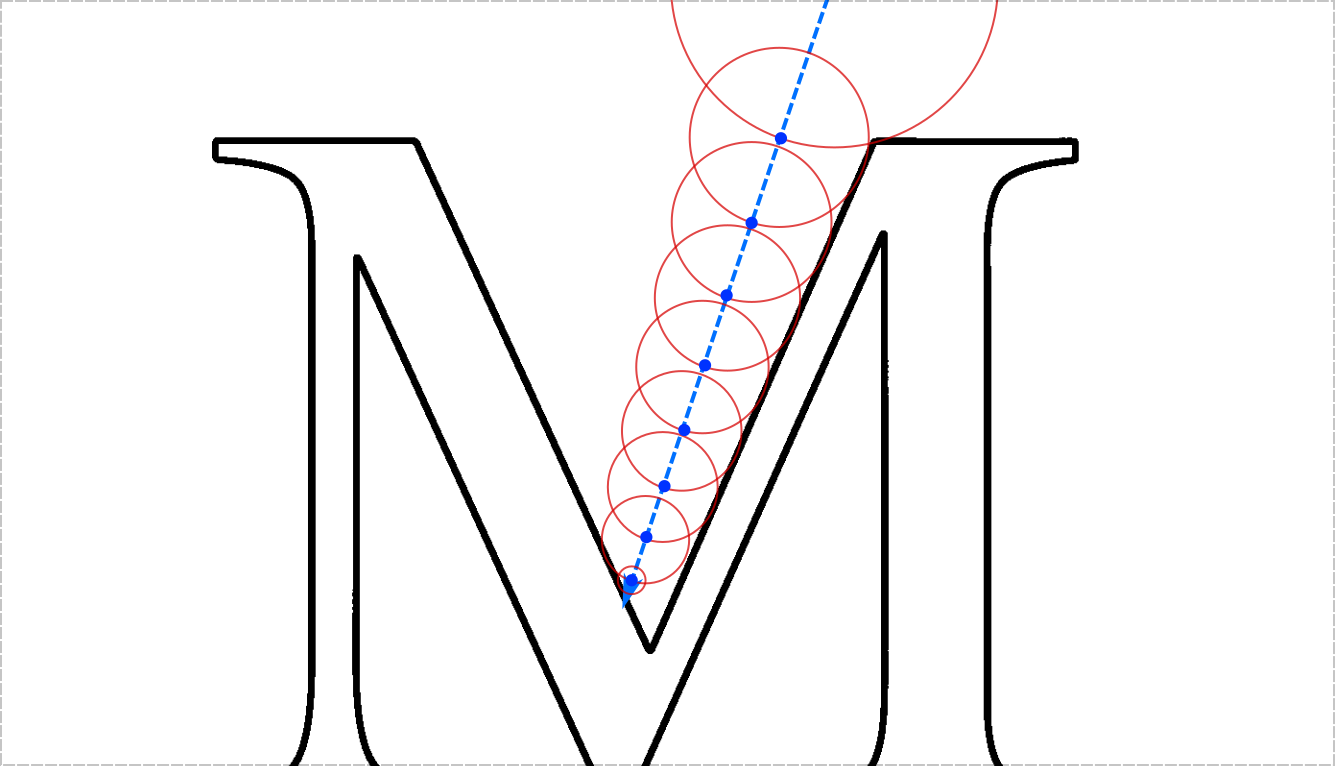
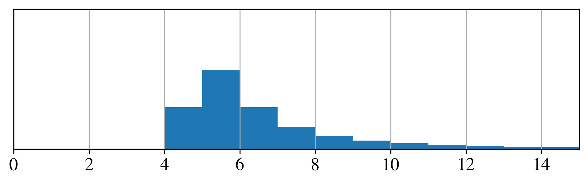
Input: Ray direction $d$ and origin $o$ Output: Position $x$ of the ray intersection with $\partial\mathcal{O}$ $x$ = $o$ repeat

      $x\leftarrow x+\Phi(x)d$

      until $|\Phi(x)|<\epsilon$;

Figure 4. Sphere tracing – (bottom) The sphere tracing algorithm introduced by (Hart, 1996) results in a long-tailed distribution of iterations when rendering 3D scenes (middle). This is caused by pathological configurations where rays graze the surface of objects (top). Note the histogram is computed across all of our 3D test scenes, and the 2D example is illustrative in purpose.

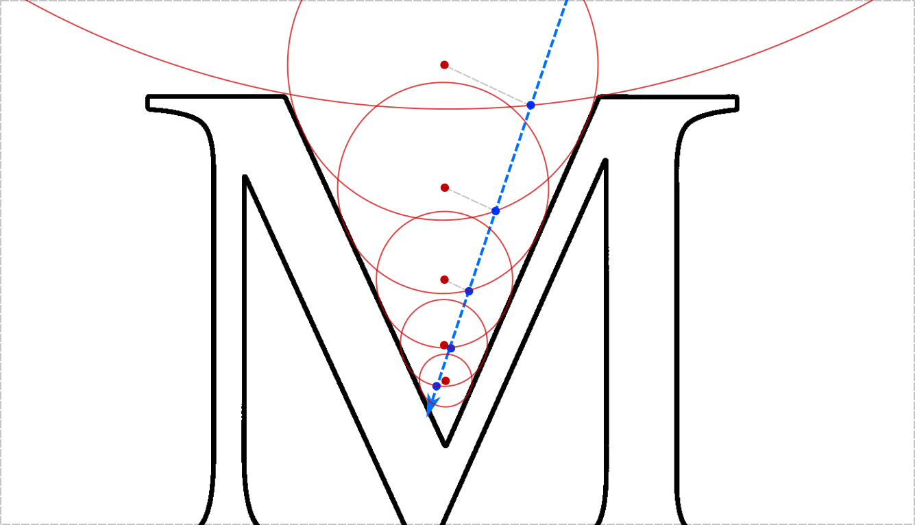
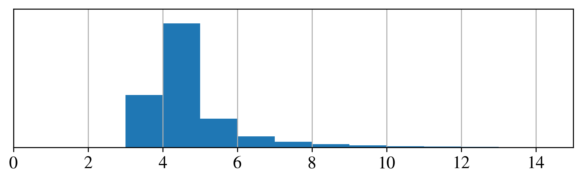
Input: Ray direction $d$ and origin $o$ Output: Position $x$ of the ray intersection with $\partial\mathcal{O}$ $x$ = $o$ repeat

      $\mathrm{proj}_{\mathcal{M}}(x)$ = $x+\nabla|\Phi(x)|(M(x)-|\Phi(x)|)$
$\beta$ = $(\mathrm{proj}_{\mathcal{M}}-x)\cdot d$
$\alpha$ = $\sqrt{\beta^{2}-(||\mathrm{proj}_{\mathcal{M}}(x)-x||_{2}^{2}-M(x)^{2})}$
$s$ = $\alpha+\beta$
$x\leftarrow x+sd$

      until $|\Phi(x)|<\epsilon$;

Figure 5. Medial sphere tracing – Our algorithm exploits the medial field to use larger spheres to advance tracing along the ray. As such, the expected number of query iterations is smaller and its distribution has a much shorter tail, leading to faster render time. Note the histogram is computed across all of our 3D test scenes, and the 2D example is illustrative in purpose.

4. Applications

4.1. Rendering implicits

An algorithm frequently used in conjunction with SDF representations is sphere tracing (Hart, 1996). The SDF representations ensure that for any point $x$ in space, a sphere centered at $x$ with radius $|\Phi(x)|$ does not cross the surface. As such, the SDF value can be used to bound the step size of a ray-marching algorithm in a way that guarantees that overstepping will not occur. In many cases, such as the case of a ray pointed directly orthogonal to a flat surface, sphere tracing will converge in one or very few iterations, making it an attractive option for rendering which is frequently used in applications that handle implicit surfaces (Seyb et al., 2019; Sitzmann et al., 2019; Yariv et al., 2020; Oechsle et al., 2021; Takikawa et al., 2021). However, there are pathological cases in which sphere tracing may take arbitrarily many iterations for a ray to converge. An example is shown in Figure 4, in which the step sizes become very small as the ray passes close to a surface which it does not intersect.

Medial sphere tracing

To address this shortcoming of the sphere tracing algorithm, we propose a modification that takes advantage of the additional information encoded in the medial field. Standard sphere tracing does not take advantage of the direction of a ray to avoid cases where the step size should not approach zero near the surface, as all queried spheres are centered on the query point. Medial spheres, on the other hand, do not suffer this limitation. As a query point $x$ approaches a smooth surface, the projected medial sphere centered at $\mathrm{proj}_{\mathcal{M}}(x)$ will approach a non-zero radius that depends on the local thickness of the shape’s complement in the region containing $x$. By using the medial sphere to advance the ray-marching process, many pathological situations in sphere tracing can be avoided; see Figure 5.

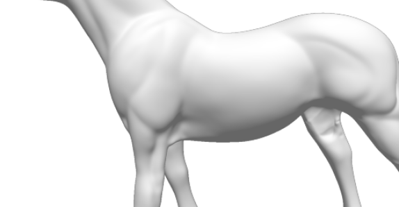
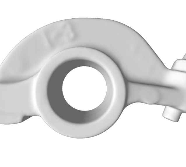
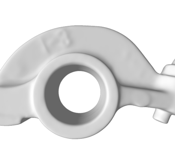
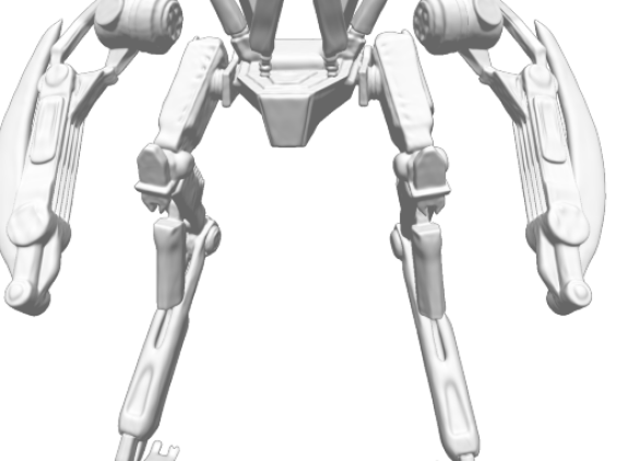
Scene	Naive Sphere Tracing			Medial Sphere Tracing
	Mean	Min	Max	Mean	Min	Max
armadillo	7.1	6.5	8.2	4.7	4.3	5.1
bunny	7.4	6.7	8.3	4.5	4.2	4.8
horse	6.5	6.0	7.3	4.1	3.8	4.5
lucy	6.1	5.6	6.9	4.1	3.8	4.5
mecha	6.9	6.3	7.8	4.8	4.4	5.2
rocker-arm	6.0	5.6	6.5	3.7	3.5	4.0

Figure 6. Rendering implicits – Three of the six scenes used for our evaluation rendered by (top-left) naive tracing and (top-right) medial tracing; note the rendered images are visually indistinguishable. (bottom) Our quantitative analysis reporting statistics about the average number of tracing iterations when rendering a frame for “naive” (left) vs. “medial” (right) sphere tracing.

Evaluation

To evaluate the efficacy of our proposed improvement to the sphere tracing algorithm, we perform experiments measuring the impact on the number of iterations taken for rays to converge to the surface. For this purpose, we train our model on a set of 3D shapes and render each from a random distribution of camera poses. As shown in Figure 6, we find that the medial sphere tracing algorithm yields significantly better worst-case performance compared to the naive algorithm for both iteration counts and render times. We also analyze the distribution of iterations required to reach convergence for each ray and plot the resulting histograms in Figure 4 and Figure 5. The histogram for the modified algorithm shows a much higher fraction of rays which converge in fewer than 6 iterations, as well as a much smaller tail of rays which take many iterations to converge. Notice that the quality of the traced image is visually equivalent to the one produced by classical SDF; see Figure 6.

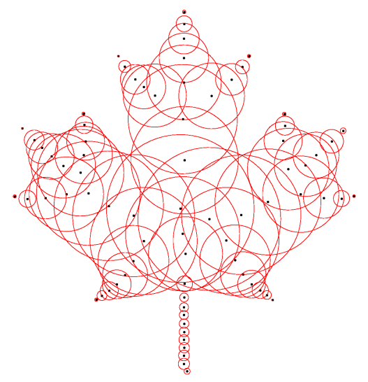
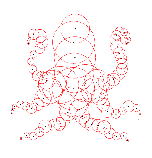
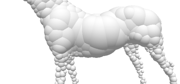
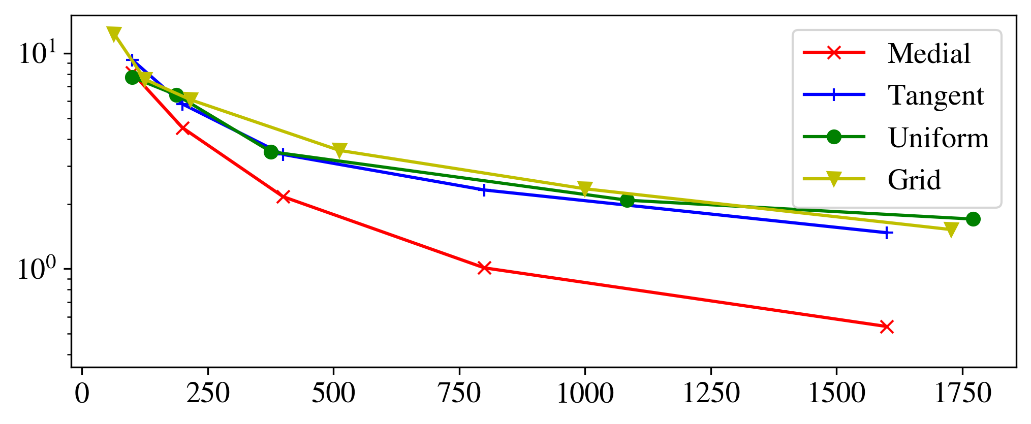
Figure 7. Physics collision proxies – Spherical (circular) shape approximation computed by the medial field in 2D (top) and in 3D (middle). We also quantitatively analyze a variety of collision proxies, revealing the corresponding memory/accuracy trade-off in percentage MAE vs memory in # of floats (bottom).

4.2. Physics proxy generation

Collision detection, and the computation of the corresponding collision response lie at the foundation of real-time physics simulation. In a modern simulation package such as NVIDIA PhysX (Macklin et al., 2014, 2020), we find that a set of spheres is used as a compact approximation of geometry for collision detection. At the same time, storing the gradient of the SDF at the sphere origin location provides the necessary meta-information to compute the collision response vector. Representing all solid objects within a scene as collection of spheres (i.e. particles) is convenient, as the complexity of collision response source code increases quadratically in the number of physical proxies that are used. While Macklin et al. (2014) employs a uniform grid of spheres to approximate the geometry, we reckon this might not be optimal (e.g. to represent the geometry of a simple spherical object with precision $\varepsilon$ we would still need $O(\varepsilon^{-d})$ primitives. The fundamental question we ask is “How can we approximate an object with fewer, larger spheres, rather than many smaller ones?” Towards this objective, we exploit the medial axis via its “maximally inscribed spheres” interpretation, together with the fact that we store their properties implicitly within our medial field.

Furthest sphere sampling

To create physics proxies we propose an algorithm that could be understood as a generalization of the furthest point sampling (Mitchell, 1991), but for spherical data. We start by placing $N$ points randomly throughout the volume and for each of these points finding a corresponding point on the medial axis, in constant time using the medial projection operation in (5). We then draw $M{<}N$ sample points $x_{n}^{*}$ through an iterative sampling:

(12) $$x_{n}^{*}=\operatorname*{arg\,max}_{x_{n}}\min_{x_{m}}\underbrace{{||x_{n}-x_{m}||}/{(r_{n}+r_{m}+\epsilon})}_{\text{normalized separation}}\;.$$

Here, $\epsilon$ prevents the selection of small, geometrically irrelevant spheres, and the normalization provides scale invariance: with $\epsilon=0$, note that two spheres of the same size that touch tangentially have a normalized separation equal to one, and this remains the case as we double their size. This algorithm results in a set of spheres that greedily minimise overlap with each other, and by virtue of them being medial spheres, are locally maximal, and represent as much volume as possible.

Evaluation

We evaluate the effectiveness of a number of approximations by comparing the representation accuracy (i.e. surface MAE) vs. memory consumption (# floats). We construct spherical proxies for a set of 3D shapes using \raisebox{-.6pt}{1}⃝ medial spheres, \raisebox{-.6pt}{2}⃝ tangent spheres, \raisebox{-.6pt}{3}⃝ uniform spheres, as well as an SDF discretization (as a collision detection event can be computed by just checking whether $\Phi(x){<}0$ for a query point $x$). The tangent spheres are sampled uniformly, and use radii provided by the SDF. The uniform spheres are sampled on a regular grid, and use a radius bounded by the width of the grid cells. The SDF grid also uses a regular grid, but represents the surface by interpolating the SDF values at the grid corners. We find that for a fixed memory budget, the medial spheres computed from the medial field provide the most accurate surface representation; see Figure 7 (bottom).

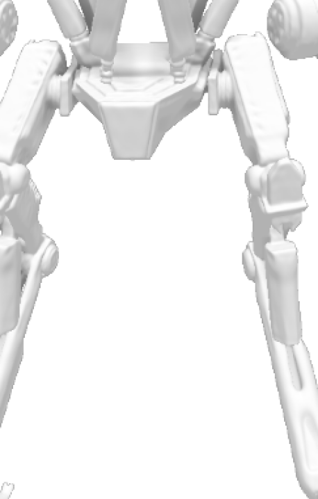
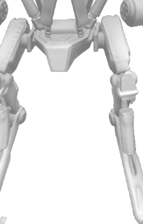
Figure 8. Ambient occlusion – Given a smooth-shaded model (top), we visualize classical “screen space ambient occlusion” (middle) as well as “local medial field ambient occlusion” (bottom). In comparison to SSAO, MFAO captures occlusion at a range defined by the parameters, without dependence on the viewpoint, and without requiring neither sampling nor filtering. Examples rendered with MFAO constants $p=0.2$ and $a=1.5$.

4.3. Ambient occlusion

Ambient occlusion is used to increase realism in rendering by modulating ambient lighting by the fraction of views into the surrounding environment that are occluded by local geometry (Pharr and Green, 2004). Computing this value correctly requires integrating over all rays leaving a point on the surface, which can have significant cost for even moderately complicated geometry. Therefore, it is often approximated by a variety of methods which provide visually similar results at substantially lower computational cost (Bavoil and Sainz, 2008).

Screen-space ambient occlusion (SSAO)

One popular example of efficient ambient occlusion approximation is screen-space ambient occlusion, which computes it using the fraction of depth values in the region of the screen surrounding a point that are smaller than the query point’s depth (Bavoil and Sainz, 2008). Note SSAO is a deferred rendering technique, as it requires the depth map to be rasterized first, and as it is based on random sampling it needs a secondary de-noising phase to remove noise. Further, as its outcome is view-dependent, the visual appearance of SSAO is not necessarily stable with respect to viewpoint variations.

Medial field ambient occlusion (MFAO)

We introduce medial field ambient occlusion as an efficient alternative to approximate ambient occlusion whenever an O(1) medial field is readily available. The medial field provides information about “local shape thickness” of both the shape, and more importantly for this application, its complement space $\mathcal{O}^{+}$. We employ the medial field to measure the local thickness of the shape complement, and derive from this value a proxy for local occlusion at a surface point $x$:

(13) $$MFAO(x)=\min(aM(x+\nabla\Phi(x)\epsilon)^{p},1)\;,$$

where $p$ and $a$ are parameters that control the strength of the effect, and $\epsilon$ is a small offset to ensure that the sampled point is in the shape complement $\mathcal{O}^{+}$. Similarly to SSAO, this method is local, in that it does not consider the effect of distant geometry, but behaves as expected in providing modulation of the ambient lighting in concave areas of the surface.

Analysis

We qualitatively compare MFAO to SSAO in Figure 8. Because both methods aim only to emulate the appearance of real ambient occlusion, and make no effort to approximate it in a mathematical sense, there is no meaningful way to perform a quantitative comparison. Nonetheless, MFAO has some immediate advantages when compared to SSAO: \raisebox{-.6pt}{1}⃝ as it does not require random sampling in its computation, it also does not requires a smoothing post-processing step to remove noise; \raisebox{-.6pt}{2}⃝ unlike SSAO, which is by its nature view-dependent, it depends only on the medial field value evaluated near the surface, and is therefore stable and consistent as the viewpoint changes.

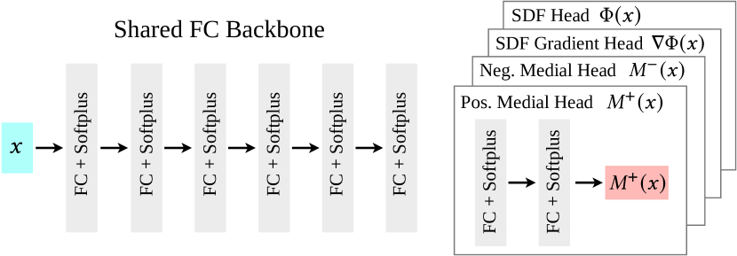
Figure 9. Architecture – A block diagram of our network architecture. A shared fully connected backbone (left) embeds a world coordinate into a learned feature, which is then decoded into $M^{+}(x)$, $\Phi(x)$, $M^{-}(x)$ and $\nabla\Phi(x)$ by four separate, fully connected heads.

5. Implementation

The typical structure for a neural SDF is, as in (Chen and Zhang, 2019; Park et al., 2019), a multi-layer perceptron (MLP) network operating on the coordinates of an input point (or an encoded version of it). Because our constraint formulation for $M(x)$ requires a way to compute $\Phi(x)$ and $\nabla\Phi(x)$, we opt to extend a neural SDF architecture to also predict $M(x)$ in addition to the typical $\Phi(x)$. We then have the option to compute $\nabla\Phi(x)$ by back-propagation, or to additionally predict it as an output.

Multi-headed architecture

We employ a multi-headed network architecture with a shared backbone; see Figure 9. Specifically, we opt for a single MLP to model all values that we wish to regress, which shares a common computation path to build a deep feature that is translated by a dedicated MLP head to either the medial field $M(x)$, the SDF $\Phi(x)$, or the gradient of the SDF $\nabla\Phi(x)$.

Modeling a discontinuous field

The medial field has a discontinuity at the surface $\partial\mathcal{O}$, which cannot be approximated by ordinary MLPs because they are Lipschitz in the inputs, and learning with gradient-based methods is biased towards small Lipschitz constants (Bartlett et al., 2017; Rahaman et al., 2019). To resolve this issue, we define two components of the medial field: $M^{-}(x)$ and $M^{+}(x)$, which are defined for $x\in\mathcal{O}^{-}$ and $x\in\mathcal{O}^{+}$ respectively. We predict the values of these fields separately with different heads, and combine them to produce $M(x)$:

(14) $$M(x)=\begin{cases}M^{+}(x)&\Phi(x)>0\\ M^{-}(x)&\Phi(x)<0\end{cases}\;.$$

This makes it possible to model the discontinuity on $\partial\mathcal{O}$ even though the outputs of all heads are Lipschitz in the input coordinates.

2D	SDF	DMF
giraffe	0.018	0.032
koch	0.051	0.055
m	0.017	0.024
maple	0.016	0.014
octopus	0.020	0.024
statue	0.017	0.020

3D	SDF	DMF
armadillo	0.045	0.043
bunny	0.040	0.032
horse	0.022	0.023
lucy	0.048	0.051
mecha	0.071	0.072
rocker-arm	0.028	0.035

Table 1. Interference analysis – We analyze whether adding the losses needed to train DMF to classical SDF training degrades the surface approximation quality. Values are mean absolute error expressed as a percentage of the bounding box diagonal.

5.1. Interference analysis – Table 1

To evaluate the effect of adding our medial field-specific losses and/or network components, we perform experiments for a collection of 2D and 3D shapes that measure the accuracy of the resulting surface representations. Specifically, for each shape we train our DMF model, as well as an equivalent neural SDF model with the medial field-specific losses omitted. We find that the addition of the medial field-related elements does not substantially affect the reconstruction quality of the network. In fact, the differences in quality are substantially below the inter-shape variation and might be entirely explained by the stochastic nature of training.

5.2. Training details

We adopt a similar neural SDF architecture to (Gropp et al., 2020). The core of the network is an MLP, operating on the encoded position, with 6 hidden layers using the geometric initialization and activation described in (Gropp et al., 2020). We then transform the resulting feature representation into $\Phi(x)\in\mathbb{R}^{1}$, $M^{+}(x)\in\mathbb{R}^{1}$, $M^{-}(x)\in\mathbb{R}^{1}$, and $\nabla\Phi(x)\in\mathbb{R}^{3}$ via dedicated two-layer MLPs (heads), each consisting of two hidden layers with 64 neurons and the same activations as the core, with a final output linear layer. We differ from (Gropp et al., 2020) in that we take as input coordinates transformed into random Fourier features (Tancik et al., 2020) composed of 64 bands, in addition to the un-transformed coordinates. To make this compatible with the geometric initialization, we weight the Fourier features using $w_{i}=\alpha||f_{i}||$, where $\alpha$ is a small constant that we set to $10^{-3}$, and $||f_{i}||$ is the frequency of the $i$-th band, so as to preserve the network’s bias towards a spherical topology. To provide supervision for the SDF predictions we use the surface and normal reconstruction loss:

(15) $$\mathcal{L}_{\textrm{surface}} =\mathds{E}_{x\sim\partial\mathcal{O}}\left[\Phi(x)^{2}\right]\;,$$

(16) $$\mathcal{L}_{\textrm{normal}} =\mathds{E}_{x\sim\partial\mathcal{O}}\left[(\nabla\Phi(x)-\nabla\Phi_{\textrm{GT}}(x))^{2}\right]\;,$$

Where $x\sim\partial\mathcal{O}$ are samples drawn uniformly from the ground-truth surface. To supervise the behaviour of the SDF in the volume we use the Eikonal loss (Gropp et al., 2020):

(17) $$\mathcal{L}_{\textrm{Eikonal}}=\mathds{E}_{x\sim\mathbb{R}^{d}}\left[(||\nabla\Phi(x)||-1)^{2}\right]\;,$$

Additionally, we employ two regularizers to improve the quality of the predicted surface and prevent the inclusion of Fourier features from interfering with the implicit SDF training:

(18) $$\mathcal{L}_{\textrm{minsurface}} =\mathds{E}_{x\sim\mathbb{R}^{d}}\left[e^{-100|\Phi(x)|}\right]\;,$$

(19) $$\mathcal{L}_{\textrm{curvature}} =\mathds{E}_{x\sim\mathbb{R}^{d}}\left[\left\|\frac{\partial}{\partial t}\nabla\Phi(x+t\nabla\Phi(x))\right\|_{1}\right]\;.$$

To speed up the execution of medial sphere tracing, which requires the gradient $\nabla\Phi(x)$ at each query point, we predict the value directly with one of the network heads and constrain it to match the analytic value found through back-propagation:

(20) $$\mathcal{L}_{\textrm{gradient}}=\mathds{E}_{x\sim\mathbb{R}^{d}}\left[||\nabla\Phi(x)-\nabla_{\textrm{analytic}}\Phi(x)||^{2}\right]\;,$$

$\mathcal{L}_{\textrm{surface}}$	$\mathcal{L}_{\textrm{normal}}$	$\mathcal{L}_{\textrm{maximal}}$	$\mathcal{L}_{\textrm{inscribed}}$	$\mathcal{L}_{\textrm{orthogonal}}$	$\mathcal{L}_{\textrm{Eikonal}}$	$\mathcal{L}_{\textrm{minsurface}}$	$\mathcal{L}_{\textrm{curvature}}$	$\mathcal{L}_{\textrm{gradient}}$
$10^{4}$	$10$	$10^{2}$	$5\times 10^{2}$	$3\times 10^{-2}$	$1$	$1$	$10^{-(1+4t)}$	$1$

Table 2. Hyperparameter setup – Determined empirically to balance the range of terms. We also schedule the curvature loss term during training (denoted here with $t$, a value varying linearly from 0 to 1 over the course of training) in order to strongly regularize at the beginning to avoid local optimum, and allow a closer fit to the surface near the end.

Training setup

For all networks we train and evaluate we use the same training setup. We use the Adam optimizer (Kingma and Ba, 2015) with the default parameters and a batch size of $2^{13}$. Our complete loss function is a weighted summation of all losses, with empirically determined hyperparameters that provide smooth optimization for all loss terms in Table 2. As some of our losses depend on point on surfaces $x{\sim}\partial\mathcal{O}$ and others on points in the rendering volume $x{\sim}\mathbb{R}^{d}$ we need different sampling strategies to account for this. To form batches of surface points we sample uniformly over the input surface mesh, using the triangle normals to provide $\nabla\Phi_{\textrm{GT}}(x)$. To form batches of points from $\mathbb{R}^{d}$ we augment the surface samples with an offset from an isotropic Gaussian distribution with $\frac{1}{2}\sigma$ equal to the bounding box diagonal. We train our network until full convergence, which takes around 500k–900k iterations for each run, taking on average 6 hours/model.

6. Conclusions

We have introduced medial fields, an implicit representation of the local thickness, that expands the capacity of implicit representations for 3D geometry. We have shown how medial fields could be stored within the parameters of a deep neural network, not only allowing O(1) access, but providing an effective strategy for its computation. We have also demonstrated the potential of medial fields by showing their use in a number of applications: we show that it can be used to \raisebox{-.6pt}{1}⃝ improve convergence when sphere tracing, \raisebox{-.6pt}{2}⃝ efficiently provide physics proxies, and \raisebox{-.6pt}{3}⃝ perform ambient occlusion.

Limitations and future works

While our method is presented as dependent on signed distance fields, this is only required to resolve the surface discontinuity in $M(x)$, and this requirement could be alleviated with an alternate approach to modelling the discontinuity. Similarly to sphere tracing, medial sphere tracing can result in rendering artifacts when the underlying field values are not accurate. This manifests in the case where queried “empty” spheres are not actually empty, resulting in the tracing stepping over the surface. Similarly to sphere tracing, this can be mitigated by assuming that the field values are over-estimated and scaling down the spheres, but doing this excessively this will begin to erode the advantage of using medial spheres. There have been other proposed modifications to sphere tracing which address pathological cases using heuristics (Bálint and Valasek, 2018; Korndörfer et al., 2014), and it could be beneficial to combine these with the additional information from medial spheres to compound the benefit to convergence. Coarse-to-fine rendering schemes could also potentially see significant improvement from medial spheres, as they do not approach zero radius near the surface, and would therefore delay subdivision of the ray packets. Computing spherical physics proxies might not be optimal for geometry exhibiting very thin geometry, or be simply unsuitable for non-orientable or non-watertight surfaces (Chibane et al., 2020). Further, while our physics proxy algorithm is a heuristic, a venue for future work is the investigation of optimization-based techniques that are capable of building proxies with guarantees on the achieved approximation power (e.g. bounded Hausdorff error), or optimal placement for a fixed cardinality of proxies.

Appendix A Proof

In this section we prove the following (recall that $\mathbf{d}(x)=|\Phi(x)|$):

Proposition A.1.

Let $M^{*}$ be a function on $\mathbb{R}^{d}\setminus\partial\mathcal{O}$ such that:

$$M^{*}(x)\geq\mathbf{d}(x)\quad \forall x\in\mathbb{R}^{d}\setminus\partial\mathcal{O}\;,$$

$$M^{*}(x)=\mathbf{d}\left(x+(M^{*}(x)-\mathbf{d}(x))\nabla\mathbf{d}(x)\right)\quad \forall x\in\mathbb{R}^{d}\setminus\partial\mathcal{O}\;,$$

$$\nabla M^{*}(x)\cdot\nabla\Phi(x)=0\quad \forall x\in\mathbb{R}^{d}\setminus(\partial\mathcal{O}\cup\mathcal{M})\;,$$

Then $M^{*}(x)=M(x)$ where $M$ is the median field of $\mathcal{O}$.

Proof.

Let $\mathbf{s}(x)$ be the spoke, i.e. the line segment connecting $\mathrm{proj}_{\mathcal{O}}(x)=x_{0}$ to $\mathrm{proj}_{\mathcal{M}}(x)$. We can parametrize this line by

$$\mathbf{s}(x)=\{x_{0}+t\nabla\mathbf{d}(x)\,|\,\text{ for }t\in\left(0,M(x)\right)\}\;.$$

Consider $f(t)=\mathbf{d}(x_{0}+t\nabla\mathbf{d}(x))$. Note that since $\mathbf{d}(x)$ is differentiable on $\mathbf{s}(x)$, we can use chain rule to get $f^{\prime}(t)=\|\nabla\mathbf{d}(x)\|^{2}=1$ for all $t\in\left(0,M(x)\right)$. Therefore $\mathbf{d}(x_{0}+t\nabla\mathbf{d}(x))=t$ for $t\in(0,M(x))$. Similarly, let $g(t)=M^{*}(x_{0}+t\nabla\mathbf{d}(x))$, and since we are asssuming $\nabla M^{*}(x)\cdot\nabla\Phi(x)=0$, we get $g^{\prime}(t)=0$, which implies $M^{*}(x)$ is constant on $\mathbf{s}(x)$. Recall that we’re assuming that $M^{*}(x)\geq\mathbf{d}(x)$. Restricting this inequality to $\mathbf{s}(x)$ we get

$$M^{*}(x)=M^{*}(x_{0}+t\nabla\mathbf{d}(x))\geq\mathbf{d}(x_{0}+t\nabla\mathbf{d}(x))=t\;,$$

for all $t\in(0,M(x))$; therefore we get $M^{*}(x)\geq M(x)$. Finally, note that $x_{0}+M(x)\nabla\mathbf{d}(x)\in\mathcal{M}$. If $M(x)>M^{*}(x)$ then, using the assumption that $M^{*}(x)=\mathbf{d}(x+(M^{*}(x)-\mathbf{d}(x))\nabla\mathbf{d}(x))$:

$$M^{*}(x) =\mathbf{d}\left(x+(M^{*}(x)-\mathbf{d}(x))\nabla\mathbf{d}(x)\right)$$

$$=\mathbf{d}\left(x_{0}+M^{*}(x)\nabla\mathbf{d}(x)\right)$$

$$=\mathbf{d}\left(x_{0}+M(x)\nabla\mathbf{d}(x)+(M^{*}(x)-M(x))\nabla\mathbf{d}(x)\right)$$

$$<\mathbf{d}\left(x_{0}+M(x)\nabla\mathbf{d}(x)\right)+\|(M^{*}(x)-M(x))\nabla\mathbf{d}(X)\|$$

$$=M^{*}(x)\;,$$

which is a contradiction. Therefore $M(x)=M^{*}(x)$ as desired. ∎

References

- (1)
- Angles et al. (2019) Baptiste Angles, Daniel Rebain, Miles Macklin, Brian Wyvill, Loic Barthe, John Lewis, Javier von der Pahlen, Shahram Izadi, Julien Valentin, Sofien Bouaziz, and Andrea Tagliasacchi. 2019. VIPER: Volume Invariant Position-based Elastic Rods. Proc. of SCA (2019).
- Atzmon and Lipman (2020) Matan Atzmon and Yaron Lipman. 2020. Sal: Sign agnostic learning of shapes from raw data. Proc. CVPR (2020).
- Bálint and Valasek (2018) Csaba Bálint and Gábor Valasek. 2018. Accelerating Sphere Tracing. Eurographics (Short Papers) (2018).
- Bartlett et al. (2017) Peter L Bartlett, Dylan J Foster, and Matus J Telgarsky. 2017. Spectrally-normalized margin bounds for neural networks. Proc. NeurIPS (2017).
- Bavoil and Sainz (2008) Louis Bavoil and Miguel Sainz. 2008. Screen space ambient occlusion. NVIDIA developer information (2008).
- Blinn (1982) James F Blinn. 1982. A generalization of algebraic surface drawing. ACM TOG (1982).
- Bloomenthal et al. (1997) Jules Bloomenthal, Chandrajit Bajaj, Jim Blinn, Brian Wyvill, Marie-Paule Cani, Alyn Rockwood, and Geoff Wyvill. 1997. Introduction to implicit surfaces. M.K.
- Blum et al. (1967) Harry Blum et al. 1967. A transformation for extracting new descriptors of shape. MIT press Cambridge.
- Bradbury et al. (2018) James Bradbury, Roy Frostig, Peter Hawkins, Matthew James Johnson, Chris Leary, Dougal Maclaurin, George Necula, Adam Paszke, Jake VanderPlas, Skye Wanderman-Milne, and Qiao Zhang. 2018. JAX: composable transformations of Python+NumPy programs. http://github.com/google/jax
- Chabra et al. (2020) Rohan Chabra, Jan Eric Lenssen, Eddy Ilg, Tanner Schmidt, Julian Straub, Steven Lovegrove, and Richard Newcombe. 2020. Deep Local Shapes: Learning Local SDF Priors for Detailed 3D Reconstruction. arXiv preprint arXiv:2003.10983 (2020).
- Chen and Zhang (2019) Zhiqin Chen and Hao Zhang. 2019. Learning implicit fields for generative shape modeling. Proc. CVPR (2019), 5939–5948.
- Chibane et al. (2020) Julian Chibane, Aymen Mir, and Gerard Pons-Moll. 2020. Neural Unsigned Distance Fields for Implicit Function Learning. Proc. NeurIPS (December 2020).
- Ericson (2004) Christer Ericson. 2004. Real-time collision detection. CRC Press.
- Genova et al. (2019) Kyle Genova, Forrester Cole, Daniel Vlasic, Aaron Sarna, William T Freeman, and Thomas Funkhouser. 2019. Learning shape templates with structured implicit functions. Proc. ICCV (2019).
- Gropp et al. (2020) Amos Gropp, Lior Yariv, Niv Haim, Matan Atzmon, and Yaron Lipman. 2020. Implicit geometric regularization for learning shapes. Proc. ICML (2020).
- Hart (1996) John C Hart. 1996. Sphere tracing: A geometric method for the antialiased ray tracing of implicit surfaces. The Visual Computer (1996).
- Hu et al. (2019) Jianwei Hu, Bin Wang, Lihui Qian, Yiling Pan, Xiaohu Guo, Lingjie Liu, and Wenping Wang. 2019. MAT-Net: Medial Axis Transform Network for 3D Object Recognition. IJCAI (2019).
- Jiang et al. (2020) Chiyu Jiang, Avneesh Sud, Ameesh Makadia, Jingwei Huang, Matthias Nießner, and Thomas Funkhouser. 2020. Local implicit grid representations for 3d scenes. Proc. CVPR (2020).
- Kingma and Ba (2015) Diederik P. Kingma and Jimmy Ba. 2015. Adam: A Method for Stochastic Optimisation. Proc. ICLR (2015).
- Korndörfer et al. (2014) Benjamin Korndörfer, Johann Keinert Henry Schäfer, Urs Ganse, and Marc Stamminger. 2014. Enhanced sphere tracing. STAG (2014).
- Liu et al. (2020) Shaohui Liu, Yinda Zhang, Songyou Peng, Boxin Shi, Marc Pollefeys, and Zhaopeng Cui. 2020. Dist: Rendering deep implicit signed distance function with differentiable sphere tracing. Proc. CVPR (2020).
- Ma et al. (2020) Baorui Ma, Zhizhong Han, Yu-Shen Liu, and Matthias Zwicker. 2020. Neural-Pull: Learning Signed Distance Functions from Point Clouds by Learning to Pull Space onto Surfaces. arXiv preprint arXiv:2011.13495 (2020).
- Macklin et al. (2020) Miles Macklin, Kenny Erleben, Matthias Müller, Nuttapong Chentanez, Stefan Jeschke, and Zach Corse. 2020. Local Optimization for Robust Signed Distance Field Collision. Proc. SIGGRAPH (2020).
- Macklin et al. (2014) Miles Macklin, Matthias Müller, Nuttapong Chentanez, and Tae-Yong Kim. 2014. Unified particle physics for real-time applications. Proc. SIGGRAPH (2014).
- Mescheder et al. (2019) Lars Mescheder, Michael Oechsle, Michael Niemeyer, Sebastian Nowozin, and Andreas Geiger. 2019. Occupancy Networks: Learning 3D Reconstruction in Function Space. Proc. CVPR (2019).
- Michalkiewicz et al. (2019) Mateusz Michalkiewicz, Jhony K Pontes, Dominic Jack, Mahsa Baktashmotlagh, and Anders Eriksson. 2019. Implicit surface representations as layers in neural networks. Proc. ICCV (2019).
- Mildenhall et al. (2020) Ben Mildenhall, Pratul P Srinivasan, Matthew Tancik, Jonathan T Barron, Ravi Ramamoorthi, and Ren Ng. 2020. NeRF: Representing Scenes as Neural Radiance Fields for View Synthesis. Proc. ECCV (2020).
- Mitchell (1991) Don P Mitchell. 1991. Spectrally optimal sampling for distribution ray tracing. Proc. of SIGGRAPH (1991).
- Niemeyer et al. (2020) Michael Niemeyer, Lars Mescheder, Michael Oechsle, and Andreas Geiger. 2020. Differentiable Volumetric Rendering: Learning Implicit 3D Representations without 3D Supervision. Proc. CVPR (2020).
- Oechsle et al. (2019) Michael Oechsle, Lars Mescheder, Michael Niemeyer, Thilo Strauss, and Andreas Geiger. 2019. Texture fields: Learning texture representations in function space. Proc. ICCV (2019).
- Oechsle et al. (2021) Michael Oechsle, Songyou Peng, and Andreas Geiger. 2021. UNISURF: Unifying Neural Implicit Surfaces and Radiance Fields for Multi-View Reconstruction. arXiv preprint arXiv:2104.10078 (2021).
- Park et al. (2019) Jeong Joon Park, Peter Florence, Julian Straub, Richard Newcombe, and Steven Lovegrove. 2019. DeepSDF: Learning Continuous Signed Distance Functions for Shape Representation. Proc. CVPR (2019).
- Peng et al. (2020) Songyou Peng, Michael Niemeyer, Lars Mescheder, Marc Pollefeys, and Andreas Geiger. 2020. Convolutional occupancy networks. Proc. ECCV (2020).
- Pharr and Green (2004) Matt Pharr and Simon Green. 2004. Ambient occlusion. GPU Gems (2004).
- Rahaman et al. (2019) Nasim Rahaman, Aristide Baratin, Devansh Arpit, Felix Draxler, Min Lin, Fred Hamprecht, Yoshua Bengio, and Aaron Courville. 2019. On the spectral bias of neural networks. Proc. ICML (2019).
- Rebain et al. (2019) Daniel Rebain, Baptiste Angles, Julien Valentin, Nicholas Vining, Jiju Peethambaran, Shahram Izadi, and Andrea Tagliasacchi. 2019. LSMAT: least squares medial axis transform. Computer Graphics Forum (2019).
- Rebain et al. (2021) Daniel Rebain, Wei Jiang, Soroosh Yazdani, Ke Li, Kwang Moo Yi, and Andrea Tagliasacchi. 2021. DeRF: Decomposed Radiance Fields. Proc. CVPR (2021).
- Seyb et al. (2019) Dario Seyb, Alec Jacobson, Derek Nowrouzezahrai, and Wojciech Jarosz. 2019. Non-linear sphere tracing for rendering deformed signed distance fields. ACM Transactions on Graphics (2019).
- Siddiqi and Pizer (2008) Kaleem Siddiqi and Stephen Pizer. 2008. Medial representations: mathematics, algorithms and applications. Springer Science & Business Media.
- Sitzmann et al. (2020a) Vincent Sitzmann, Eric R Chan, Richard Tucker, Noah Snavely, and Gordon Wetzstein. 2020a. Metasdf: Meta-learning signed distance functions. Proc. NeurIPS (2020).
- Sitzmann et al. (2020b) Vincent Sitzmann, Julien N.P. Martel, Alexander W. Bergman, David B. Lindell, and Gordon Wetzstein. 2020b. Implicit Neural Representations with Periodic Activation Functions. Proc. NeurIPS (2020).
- Sitzmann et al. (2019) Vincent Sitzmann, Michael Zollhöfer, and Gordon Wetzstein. 2019. Scene Representation Networks: Continuous 3D-Structure-Aware Neural Scene Representations. Proc. NeurIPS (2019).
- Tagliasacchi et al. (2016) Andrea Tagliasacchi, Thomas Delame, Michela Spagnuolo, Nina Amenta, and Alexandru Telea. 2016. 3D Skeletons: A State-of-the-Art Report. Proc. Eurographics (2016).
- Takikawa et al. (2021) Towaki Takikawa, Joey Litalien, Kangxue Yin, Karsten Kreis, Charles Loop, Derek Nowrouzezahrai, Alec Jacobson, Morgan McGuire, and Sanja Fidler. 2021. Neural geometric level of detail: Real-time rendering with implicit 3D shapes. Proc. CVPR (2021).
- Tancik et al. (2020) Matthew Tancik, Pratul P Srinivasan, Ben Mildenhall, Sara Fridovich-Keil, Nithin Raghavan, Utkarsh Singhal, Ravi Ramamoorthi, Jonathan T Barron, and Ren Ng. 2020. Fourier features let networks learn high frequency functions in low dimensional domains. Proc. NeurIPS (2020).
- Thiery et al. (2013) Jean-Marc Thiery, Émilie Guy, and Tamy Boubekeur. 2013. Sphere-meshes: Shape approximation using spherical quadric error metrics. ACM TOG (2013).
- Thiery et al. (2016) Jean-Marc Thiery, Émilie Guy, Tamy Boubekeur, and Elmar Eisemann. 2016. Animated mesh approximation with sphere-meshes. ACM TOG (2016).
- Tkach et al. (2016) Anastasia Tkach, Mark Pauly, and Andrea Tagliasacchi. 2016. Sphere-Meshes for Real-Time Hand Modeling and Tracking. Proc. SIGGRAPH Asia (2016).
- Yariv et al. (2020) Lior Yariv, Yoni Kasten, Dror Moran, Meirav Galun, Matan Atzmon, Basri Ronen, and Yaron Lipman. 2020. Multiview neural surface reconstruction by disentangling geometry and appearance. Proc. NeurIPS (2020).