Vanishing Curvature and the Power of Adaptive Methods in Randomly Initialized Deep Networks

Antonio Orvieto   Jonas Kohler11footnotemark: 1   Dario PavlloThomas Hofmann   Aurelien Lucchi
Department of Computer Science
ETH Zurich
Equal contribution
Abstract

This paper revisits the so-called vanishing gradient phenomenon, which commonly occurs in deep randomly initialized neural networks. Leveraging an in-depth analysis of neural chains, we first show that vanishing gradients cannot be circumvented when the network width scales with less than O(depth)𝑂depthO(\text{depth}), even when initialized with the popular Xavier and He initializations. Second, we extend the analysis to second-order derivatives and show that random i.i.d. initialization also gives rise to Hessian matrices with eigenspectra that vanish as networks grow in depth. Whenever this happens, optimizers are initialized in a very flat, saddle point-like plateau, which is particularly hard to escape with stochastic gradient descent (SGD) as its escaping time is inversely related to curvature. We believe that this observation is crucial for fully understanding (a) historical difficulties of training deep nets with vanilla SGD, (b) the success of adaptive gradient methods (which naturally adapt to curvature and thus quickly escape flat plateaus) and (c) the effectiveness of modern architectural components like residual connections and normalization layers.

1 Introduction and related work

In the last decade, network depth has emerged as a key component for the success of modern deep learning (He et al., 2016b), providing significant improvements in terms of generalization, particularly in the field of computer vision (He et al., 2016a, b) and natural language processing (Brown et al., 2020). These benefits are mostly attributed to gains in representational power. In fact, it was shown in (Telgarsky, 2016) that there exist deep neural networks of bounded width that cannot be approximated by shallow networks, unless their layers grow exponentially wide. From an optimization perspective, however, depth introduces several problems when training after random initialization. First, in the infinite depth limit, a collapse in the rank of the network mapping prevents information propagation, which renders learning impossible (Schoenholz et al., 2016; Pennington et al., 2018; Daneshmand et al., 2020). Secondly, even in finite but large depth the so-called vanishing gradient problem commonly makes it difficult to train deep (un-normalized) networks with stochastic gradient descent (Hochreiter, 1991; Bengio et al., 1994; Pascanu et al., 2013).
Refer to caption
Refer to caption
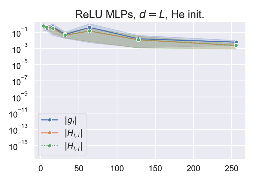
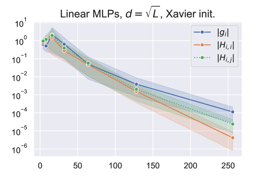
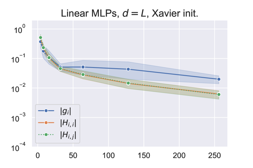
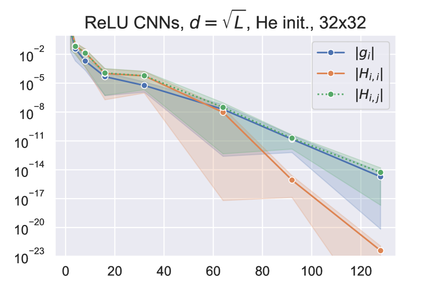
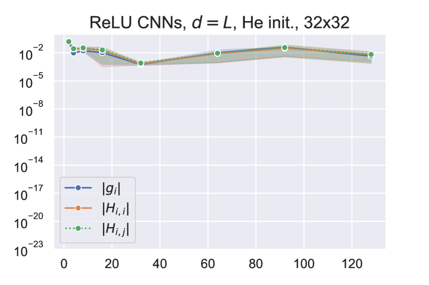
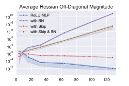
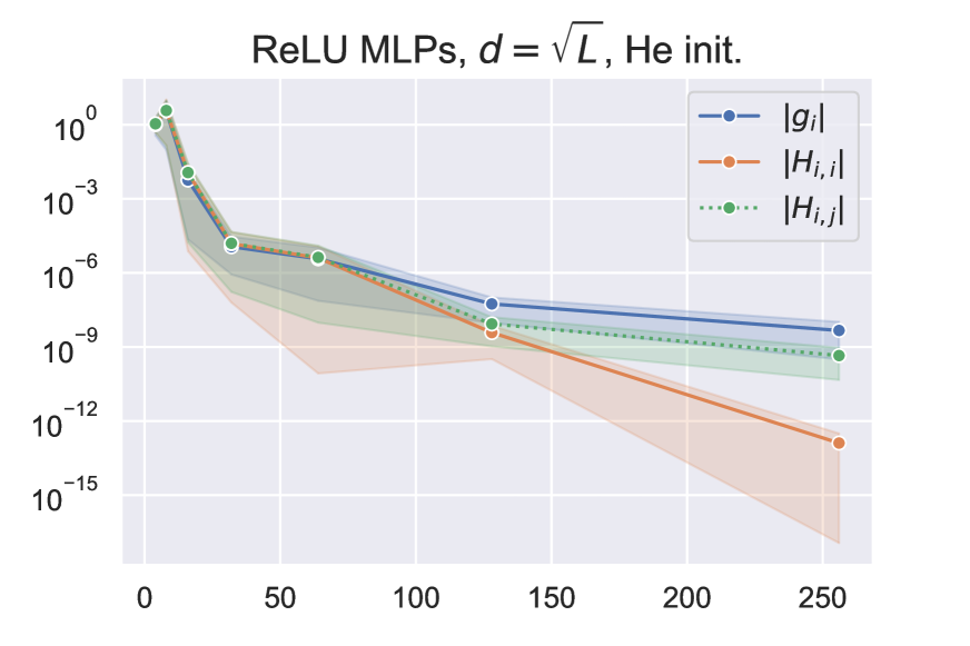
Figure 1: Effect of width in ReLU MLPs: Gradient and curvature scaling on Fashion-MNIST over depth. While quantities vanish on the left (d=L𝑑𝐿d=\sqrt{L}), the right shows stable magnitudes. Mean and 95% CI of 15 runs.

In this work, we focus on the latter setting. First, we show that networks that are deeper than wide suffer from vanishing gradients at initialization even when following the initialization schemes proposed in (Glorot & Bengio, 2010; He et al., 2015). This is somewhat surprising at first, since the analysis undertaken in these seminal works suggests stable gradient norms for any depth, in expectation. However, as we show in Section 3, the expectation analysis has an important shortcoming: When networks are deeper than wide, the initialization variance suggested to be optimal in order to stabilize the expected forward- and backpropagation norms yields exploding higher moments of these quantities. As a result, their distribution becomes fat tailed in depth and hence the expected value itself is increasingly unlikely to be observed. Thus, we instead study the median of the propagation norms, which we find to indeed vanish in depth.

Second, we reveal that, in the above settings, not only the gradient vanishes as depth increases, but also the entries of the Hessian become smaller and smaller. Hence, by Gershgorin’s theorem (Gershgorin, 1931), the eigenvalues shrink in depth. As a result, random i.i.d. initialization ends up positioning optimization methods in a very flat, saddle point like region around the origin, where gradients are small and both negative as well as positive curvature exist. This is particularly unfortunate for stochastic gradient descent (SGD) as its saddle escaping time is inversely related to the magnitude of the most negative eigenvalue (see Prop. 7 as well as (Daneshmand et al., 2018; Fang et al., 2019)). This observation complements the vanishing gradient argument, whose implications for optimization were so far rather vague since small gradients on their own are not a-priori problematic for gradient-based learning: In fact, it is often the Lipschitz constant (i.e. curvature) and not the norm of the gradients that determines the speed of convergence of gradient descent (Nesterov et al., 2018). Even around saddle points, sufficient negative curvature allows stochastic gradient descent to make fast progress despite small gradient norms.111To be more precise, the anisotropic noise of SGD has been shown to be aligned with negative curvature directions (Zhu et al., 2019; Daneshmand et al., 2018; Fang et al., 2019), which allows for a per-step progress of 𝒪(λ3)𝒪superscript𝜆3\mathcal{O}(\lambda^{3}) where λ𝜆\lambda is the curvature along the current search direction (Curtis & Robinson, 2019). Hence, vanishing gradients on their own fall short of a satisfactory description for the difficulty of training very deep networks with plain SGD.

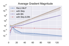
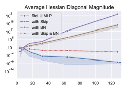
We believe that it is precisely the vanishing curvature phenomenon, combined with the deficiencies of SGD in escaping flat saddles, that lead to developments on three fronts: (i) modern architectural components: batch normalization (BN) (Ioffe & Szegedy, 2015) and residual connections (He et al., 2016a), which collectively circumvent vanishing gradients/curvature even in non-linear networks (Fig. 7). (ii) robust initialization schemes: orthogonal- (Saxe et al., 2013), which is restricted to linear networks (Fig. 14) and Fixup/Skip initialization (Zhang et al., 2019a; De & Smith, 2020), which downscale the parametric branch of residual architectures proportionally to their depth, thus trivially yielding identity mappings in the limit. (iii) Adaptive training algorithms: notably several years before the emergence of BN and residual connections, so-called adaptive gradient methods (Duchi et al., 2011; Tieleman & Hinton, 2012) have shown remarkable success in training deep networks. We believe that their increased popularity is (at least partially) attributable to the fact that adaptive gradients methods are robust to this failure mode of random i.i.d. initialization because they naturally adapt to curvature, which allows them to escape saddles in time independent of their flatness (Dauphin et al., 2015; Staib et al., 2019).

In summary, our contribution is threefold:

  • We discuss shortcomings of the analysis in Glorot & Bengio (2010); He et al. (2015) and clarify when gradients vanish even with the initialization proposed in these seminal works.

  • We enhance the understanding of the vanishing gradient phenomenon by showing that they co-occur with vanishing curvature, giving rise to flat plateaus at initialization. This effect gives a comprehensive understanding of the difficulty of training (classical) deep nets with (vanilla) SGD.

  • Finally, we link the remarkable curvature adaptation capability of adaptive gradient methods to this phenomenon and show that it allows them to optimize networks of any depth.

2 Notation and setting

In our theoretical analysis, we consider the L2 loss associated with a multilayer perceptron (MLP)

(𝐖)=12ni=1n𝐲i𝐁𝐃L𝐖ϕL:1𝐀𝐱i22,𝐖ϕL:1:=𝐖L𝐃L1𝐖L1𝐖2𝐃1𝐖1𝐃0formulae-sequence𝐖12𝑛superscriptsubscript𝑖1𝑛subscriptsuperscriptnormsubscript𝐲𝑖superscript𝐁𝐃𝐿subscriptsuperscript𝐖:𝐿1italic-ϕsubscript𝐀𝐱𝑖22assignsuperscriptsubscript𝐖italic-ϕ:𝐿1superscript𝐖𝐿superscript𝐃𝐿1superscript𝐖𝐿1superscript𝐖2superscript𝐃1superscript𝐖1superscript𝐃0\displaystyle{\mathcal{L}}({\bf W})=\frac{1}{2n}\sum_{i=1}^{n}\|{\bf y}_{i}-{\bf B}{\bf D}^{L}\mathbf{W}^{L:1}_{\phi}{\bf A}{\bf x}_{i}\|^{2}_{2},\quad{\bf W}_{\phi}^{L:1}:={\bf W}^{L}{\bf D}^{L-1}{\bf W}^{L-1}\cdots{\bf W}^{2}{\bf D}^{1}{\bf W}^{1}{\bf D}^{0} (1)

where 𝐱idin,𝐲idoutformulae-sequencesubscript𝐱𝑖superscriptsubscript𝑑𝑖𝑛subscript𝐲𝑖superscriptsubscript𝑑𝑜𝑢𝑡{\bf x}_{i}\in\mathbb{R}^{d_{in}},{\bf y}_{i}\in\mathbb{R}^{d_{out}}, 𝐀d×din𝐀superscript𝑑subscript𝑑𝑖𝑛{\bf A}\in\mathbb{R}^{d\times d_{in}},𝐁dout×d𝐁superscriptsubscript𝑑𝑜𝑢𝑡𝑑{\bf B}\in\mathbb{R}^{d_{out}\times d}, and 𝐖d×d,=1,,Lformulae-sequencesuperscript𝐖superscript𝑑𝑑for-all1𝐿{\bf W}^{\ell}\in{\mathbb{R}}^{d\times d},\forall\ell=1,\ldots,L . 𝐃superscript𝐃{\bf D}^{\ell} is the diagonal matrix of activation gates w.r.t the non-linearity ϕitalic-ϕ\phi at layer \ell, which we consider to be either ϕ(x)=xitalic-ϕ𝑥𝑥\phi(x)=x (linear networks) or ϕ(x)=max{x,0}italic-ϕ𝑥𝑥0\phi(x)=\max\{x,0\} (ReLU networks).

Assumption 1 (Random initialization).

Each entry of 𝐖superscript𝐖{\bf W}^{\ell} (=1,,L1𝐿\ell=1,\ldots,L) is initialized i.i.d. with some distribution 𝒫𝒫\mathcal{P} symmetric around zero with variance σ2<superscript𝜎2\sigma^{2}<\infty and fourth moment μ4<subscript𝜇4\mu_{4}<\infty.

For more than a decade, the standard choice of initialization variance was σ2=13dsuperscript𝜎213𝑑\sigma^{2}=\frac{1}{3d} (LeCun et al., 1998). Motivated by repeated observations of the vanishing gradient problem, an improved initialization was suggested by  (Glorot & Bengio, 2010) and (He et al., 2015). In the following, we define the parameter p=1𝑝1p=1 for the linear case and p=1/2𝑝12p=1/2 for the ReLU case.

Proposition 2 ((Glorot & Bengio, 2010), (He et al., 2015)).
Under Assumption 1, the variance of the weight gradients Var((𝐖)/𝐖)Var𝐖superscript𝐖\text{Var}(\partial{\mathcal{L}}({\bf W})/\partial{\bf W}^{\ell}) scales as (pdσ2)Lsuperscript𝑝𝑑superscript𝜎2𝐿(pd\sigma^{2})^{L} across all layers =1,,L1𝐿\ell=1,\ldots,L. When initializing with σ2=13dsuperscript𝜎213𝑑\sigma^{2}=\tfrac{1}{3d} (LeCun init.), this quantity vanishes in depth. Instead, choosing σ2=1/dsuperscript𝜎21𝑑\sigma^{2}=1/d in the linear case (Xavier init.), and σ2=2/dsuperscript𝜎22𝑑\sigma^{2}=2/d in the ReLU case (He init), stabilizes the variance.
Proof.

Let 𝐚+1=𝐖𝐡superscript𝐚1superscript𝐖superscript𝐡{\bf a}^{\ell+1}={\bf W}^{\ell}{\bf h}^{\ell} be the preactivation of layer +11\ell+1, computed using 𝐡=𝐃𝐚superscript𝐡superscript𝐃superscript𝐚{\bf h}^{\ell}={\bf D}^{\ell}{\bf a}^{\ell}, the activation at layer \ell . Let a+1superscript𝑎1a^{\ell+1}, wsuperscript𝑤w^{\ell} and hsuperscripth^{\ell} represent the random variables corresponding to each element in 𝐚+1superscript𝐚1{\bf a}^{\ell+1}, 𝐖superscript𝐖{\bf W}^{\ell} and 𝐡superscript𝐡{\bf h}^{\ell} respectively. Since wsuperscript𝑤w^{\ell} is zero mean, we have that Var[a+1]=dVar[w]𝔼[(h)2]Vardelimited-[]superscript𝑎1𝑑Vardelimited-[]superscript𝑤𝔼delimited-[]superscriptsuperscript2\text{Var}[a^{\ell+1}]=d\cdot\text{Var}[w^{\ell}]\cdot{\mathbb{E}}[(h^{\ell})^{2}]. Finally, since 𝔼[(h)2]=pVar[(a)2]𝔼delimited-[]superscriptsuperscript2𝑝Vardelimited-[]superscriptsuperscript𝑎2{\mathbb{E}}[(h^{\ell})^{2}]=p\text{Var}[(a^{\ell})^{2}] (p=1𝑝1p=1 for linear nets and 1/2121/2 for ReLU nets), we end up with Var[a+1]=dσ2pVar[a]Vardelimited-[]superscript𝑎1𝑑superscript𝜎2𝑝Vardelimited-[]superscript𝑎\text{Var}[a^{\ell+1}]=d\sigma^{2}p\cdot\text{Var}[a^{\ell}], which yields Var[a+1]=Var[a]Vardelimited-[]superscript𝑎1Vardelimited-[]superscript𝑎\text{Var}[a^{\ell+1}]=\text{Var}[a^{\ell}] for σ2=1dpsuperscript𝜎21𝑑𝑝\sigma^{2}=\frac{1}{dp}. ∎

For example, for the uniform initialization 𝒫=𝒰[τ,τ]𝒫𝒰𝜏𝜏\mathcal{P}=\mathcal{U}[-\tau,\tau], we have σ2=τ2/3superscript𝜎2superscript𝜏23\sigma^{2}=\tau^{2}/3 and hence the "optimal" initialization range amounts to τ=3/d𝜏3𝑑\tau=\sqrt{3/d} in the linear - and τ=6/d𝜏6𝑑\tau=\sqrt{6/d} in the ReLU case.

3 Vanishing in neural chains and implications for optimization

To illustrate an important shortcoming in the analyses of (Glorot & Bengio, 2010) and (He et al., 2015), we consider a deep linear network of width one (henceforth called neural chain). While these networks are utterly useless for practical applications, they are sufficient to exhibit some critical properties of the loss landscape, that generalize to wider nets (see next section).

In the neural chain case, if 𝐀=𝐁=1𝐀𝐁1{\bf A}={\bf B}=1, Eq.(1) simplifies to (𝐰)=i=1n(yiwLw1xi)2/(2n)𝐰superscriptsubscript𝑖1𝑛superscriptsubscript𝑦𝑖subscript𝑤𝐿subscript𝑤1subscript𝑥𝑖22𝑛{\mathcal{L}}({\bf w})=\sum_{i=1}^{n}(y_{i}-w_{L}...w_{1}x_{i})^{2}/(2n) and we consider each wisubscript𝑤𝑖w_{i}\in\mathbb{R} to be drawn uniformly at random in [τ,τ]𝜏𝜏[-\tau,\tau]. Prop. 2 suggests that both forward pass and gradient remain stable in magnitude when choosing τ=3𝜏3\tau=\sqrt{3}. While this is true in expectation, it is not the case when initializing individual models, where the expected value becomes an increasingly atypical event (see Thm. 6) as the chain grows in depth (L𝐿L). Indeed, in Fig. 2 we see that all quantities vanish under the “optimal” initialization. Perhaps the most intuitive indication for this pathological behavior comes from writing down the following population quantities for the absolute value of the input-output map.

Proposition 3 (Forward pass statistics chain).
Consider the absolute value of a forward pass on the chain, i.e. the random variable vτ,L:=k=1L(τwk),assignsubscript𝑣𝜏𝐿superscriptsubscriptproduct𝑘1𝐿𝜏subscript𝑤𝑘v_{\tau,L}:=\prod_{k=1}^{L}(\tau w_{k}), with wkiid𝒰(0,1]superscriptsimilar-toiidsubscript𝑤𝑘𝒰01w_{k}\stackrel{{\scriptstyle\text{iid}}}{{\sim}}\mathcal{U}(0,1]. Then, 𝔼[vτ,L]=(τ2)L,𝔼[vτ,L2]=(τ23)L,𝔼[vτ,L3]=(τ34)L.formulae-sequence𝔼delimited-[]subscript𝑣𝜏𝐿superscriptcontinued-fraction𝜏2𝐿formulae-sequence𝔼delimited-[]superscriptsubscript𝑣𝜏𝐿2superscriptcontinued-fractionsuperscript𝜏23𝐿𝔼delimited-[]superscriptsubscript𝑣𝜏𝐿3superscriptcontinued-fractionsuperscript𝜏34𝐿{\mathbb{E}}\left[v_{\tau,L}\right]=\left(\cfrac{\tau}{2}\right)^{L},\quad{\mathbb{E}}[v_{\tau,L}^{2}]=\left(\cfrac{\tau^{2}}{3}\right)^{L},\quad{\mathbb{E}}[v_{\tau,L}^{3}]=\left(\cfrac{\tau^{3}}{4}\right)^{L}. (2) Clearly, τ=3𝜏3\tau=\sqrt{3} (Xavier init.) leads to 𝔼[vτ,L]0𝔼delimited-[]subscript𝑣𝜏𝐿0{\mathbb{E}}\left[v_{\tau,L}\right]\to 0, 𝔼[vτ,L2]=1𝔼delimited-[]superscriptsubscript𝑣𝜏𝐿21{\mathbb{E}}\left[v_{\tau,L}^{2}\right]=1 and 𝔼[vτ,L3]𝔼delimited-[]superscriptsubscript𝑣𝜏𝐿3{\mathbb{E}}[v_{\tau,L}^{3}]\to\infty, as L𝐿L\to\infty.

It might be tempting to conclude from Eq. 2 that picking τ=2𝜏2\tau=2 instead of 33\sqrt{3} solves the problem. Yet, this is not the case since then 𝔼[vτ,L2]𝔼delimited-[]superscriptsubscript𝑣𝜏𝐿2{\mathbb{E}}[v_{\tau,L}^{2}]\to\infty and by Mallows inequality (Mallows & Richter, 1969) the mean becomes an unreliable predictor for the median (see Fig. 21), as their difference is bounded by one standard deviation (exploding). In fact, the above proposition reveals that one cannot stabilize any pair of moments of vτ,Lsubscript𝑣𝜏𝐿v_{\tau,L} simultaneously and hence in both cases τ=3𝜏3\tau=\sqrt{3} and τ=2𝜏2\tau=2, the distribution of vτ,Lsubscript𝑣𝜏𝐿v_{\tau,L} becomes fat-tailed as L𝐿L\to\infty, which leads to slow convergence of the central limit theorem222The speed of convergence in the CLT, as bounded by the Berry-Esseen inequality, is proportional to 𝔼[|v|3]𝔼delimited-[]superscript𝑣3{\mathbb{E}}[|v|^{3}].. As we show in Sec. 4, this basic moment trade off prevails in wider nets (see Eq. 6).

Therefore, one has to go beyond the population analysis in order to better understand this phenomenon. In a first step, we characterize the distribution of the magnitude of the input-output map in log scale.

Lemma 4 (Distribution of input-output).
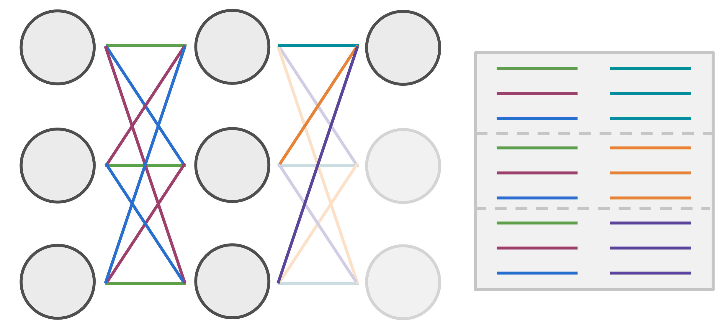
In the setting of Prop. 3, ln(vτ,L)=zLln(τ),zErlang(L,1).formulae-sequencesubscript𝑣𝜏𝐿𝑧𝐿𝜏similar-to𝑧Erlang𝐿1\displaystyle-\ln(v_{\tau,L})=z-L\ln(\tau),\quad z\sim\mathrm{Erlang}(L,1). Hence Pr(ln(vτ,L)ζ)=1eξk=0L1ξkk!Prsubscript𝑣𝜏𝐿𝜁1superscript𝑒𝜉superscriptsubscript𝑘0𝐿1superscript𝜉𝑘𝑘\operatorname{Pr}(-\ln(v_{\tau,L})\leq\zeta)=1-e^{-\xi}\sum_{k=0}^{L-1}\frac{\xi^{k}}{k!}, ξ:=ζ+Llnτassign𝜉𝜁𝐿𝜏\xi:=\zeta+L\ln\tau.
[Uncaptioned image]
Proof.

Clearly, ln(wk))-\ln(w_{k})) is exponentially distribution with parameter 111. Furthermore, if random variables VkExp(λ)similar-tosubscript𝑉𝑘Exp𝜆V_{k}\sim\mathrm{Exp}(\lambda) are independent, then k=1LVkErlang(L,λ)similar-tosuperscriptsubscript𝑘1𝐿subscript𝑉𝑘Erlang𝐿𝜆\sum_{k=1}^{L}V_{k}\sim\mathrm{Erlang}(L,\lambda) (Temme, 1996; Devroye, 2006). The CDF follows from the properties of the Erlang distribution, which concludes the proof. ∎

This allows to characterize the median and provide an asymptotic333In the context of asymptotic expansions, we write fgsimilar-to𝑓𝑔f\sim g if limLf(L)/g(L)=1subscript𝐿𝑓𝐿𝑔𝐿1\lim_{L\to\infty}f(L)/g(L)=1. bound on the forward pass norm.

Proposition 5 (Expectation is not predictive for input-output map magnitude).
We have median[vτ,L]=eLln(τ)L~,with L1/3L~L1+ln(2).formulae-sequencemediandelimited-[]subscript𝑣𝜏𝐿superscript𝑒𝐿𝜏~𝐿with 𝐿13~𝐿𝐿12\mathrm{median}\left[v_{\tau,L}\right]=e^{L\ln(\tau)-\tilde{L}},\quad\quad\text{with }L-\nicefrac{{1}}{{3}}\leq\tilde{L}\leq L-1+\ln(2). Therefore, if τ=2𝜏2\tau=2, median[vτ,L]0mediandelimited-[]subscript𝑣𝜏𝐿0\mathrm{median}\left[v_{\tau,L}\right]\to 0 while 𝔼[vτ,L]=1𝔼delimited-[]subscript𝑣𝜏𝐿1{\mathbb{E}}\left[v_{\tau,L}\right]=1 and 𝔼[vτ,L2]𝔼delimited-[]superscriptsubscript𝑣𝜏𝐿2{\mathbb{E}}\left[v_{\tau,L}^{2}\right]\to\infty. For τ=3𝜏3\tau=\sqrt{3}, also median[vτ,L]0mediandelimited-[]subscript𝑣𝜏𝐿0\mathrm{median}\left[v_{\tau,L}\right]\to 0. Yet, the median is stabilized for τ=e𝜏𝑒\tau=e, since limL(vτ,L)1L=a.s.τ/e, which implies vτ,Lexp(L(1lnτ)).\displaystyle\lim_{L\to\infty}(v_{\tau,L})^{\frac{1}{L}}\stackrel{{\scriptstyle a.s.}}{{=}}\tau/e,\ \ \text{ which implies }\quad v_{\tau,L}\sim\exp\left(-L(1-\ln\tau)\right).
Proof.

The moments follow from Prop. 3. For the median, we solve Pr(lnvτ,Lζ)=1/2Prsubscript𝑣𝜏𝐿𝜁12\operatorname{Pr}(-\ln v_{\tau,L}\leq\zeta)=1/2 for ζ𝜁\zeta, which by Lemma 4 is equivalent to solving 1eξk=0L1ξkk!=1/21superscript𝑒𝜉superscriptsubscript𝑘0𝐿1superscript𝜉𝑘𝑘121-e^{-\xi}\sum_{k=0}^{L-1}\frac{\xi^{k}}{k!}=1/2 w.r.t. ξ:=ζ+Llnτassign𝜉𝜁𝐿𝜏\xi:=\zeta+L\ln\tau. The solution, termed L~~𝐿\tilde{L}, is approximated with a Ramanujan formula (1913), as in (Choi, 1994). Since vτ,L=eLlnτzsubscript𝑣𝜏𝐿superscript𝑒𝐿𝜏𝑧v_{\tau,L}=e^{L\ln\tau-z}, then (vτ,L)1L=τez/L.superscriptsubscript𝑣𝜏𝐿1𝐿𝜏superscript𝑒𝑧𝐿(v_{\tau,L})^{\frac{1}{L}}=\tau e^{-z/L}. We conclude using the strong law of large numbers. ∎

We now apply the idea behind the last result to analyze the first and second order partial derivatives.

Theorem 6 (Almost sure vanishing).
Assume bounded data and wi𝒰[τ,τ]similar-tosubscript𝑤𝑖𝒰𝜏𝜏w_{i}\sim\mathcal{U}[-\tau,\tau], with fixed τ𝜏\tau. For each k,L𝑘𝐿k,\ell\leq L we asymptotically (as L𝐿L\to\infty) have almost surely that |chain(𝐰)wk|,|2chain(𝐰)wkwk|subscriptchain𝐰subscript𝑤𝑘superscript2subscriptchain𝐰subscript𝑤𝑘subscript𝑤𝑘\displaystyle\left|\frac{\partial{\mathcal{L}}_{\text{chain}}({\bf w})}{\partial w_{k}}\right|,\left|\frac{\partial^{2}{\mathcal{L}}_{\text{chain}}({\bf w})}{\partial w_{k}\partial w_{\ell\neq k}}\right| =𝒪(e(L1)(1lnτ)),absent𝒪superscript𝑒𝐿11𝜏\displaystyle=\mathcal{O}\left(e^{-(L-1)(1-\ln\tau)}\right), |2chain(𝐰)wkwk|superscript2subscriptchain𝐰subscript𝑤𝑘subscript𝑤𝑘\displaystyle\left|\frac{\partial^{2}{\mathcal{L}}_{\text{chain}}({\bf w})}{\partial w_{k}\partial w_{k}}\right| =𝒪(e2(L1)(1lnτ)).absent𝒪superscript𝑒2𝐿11𝜏\displaystyle=\mathcal{O}\left(e^{-2(L-1)(1-\ln\tau)}\right). In particular, as for vτ,Lsubscript𝑣𝜏𝐿v_{\tau,L}, all these quantities asymptotically vanish if τ<e𝜏𝑒\tau<e and explode if τ>e𝜏𝑒\tau>e.
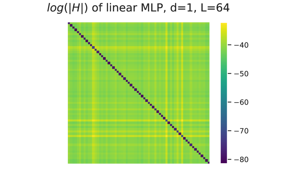
In the case of Xavier init. τ=3𝜏3\tau=\sqrt{3}, the Hessian vanishes in norm (hence eigenvalues vanish) and becomes hollow, i.e. diagonal elements become exponentially smaller than off-diagonal elements.

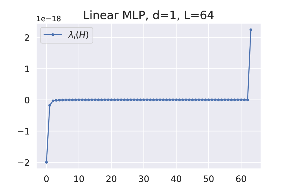
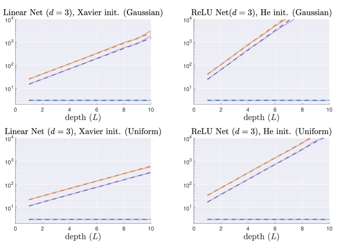
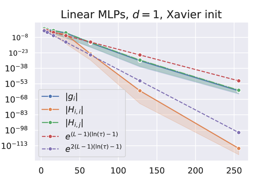
The proof is presented in App. B. Fig. 2 and Fig. 20 (top row) show that the result is very precise.
Refer to caption

depth

Refer to caption

eigenvalue index

Refer to caption
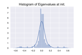
Figure 2: Left: Gradient and Hessian entry magnitudes for deep neural chains (Xavier init, Mean and 95%percent\% CI of 10 random seeds) Middle, Right: Eigenvalues and log Hessian entry maginute at init. for L=64𝐿64L=64.

Implications on landscape and optimization.

In narrow networks, our results show vanishing gradients and hollow Hessians with positive and negative eigenvalues of decreasing magnitude (also see Fig. 12). Hence, the initialization landscape constitutes a plateau that resembles a barely curved saddle (see Fig. 3). As discussed next, this is particularly bad for optimization with plain SGD but adaptive methods escape the plateau quickly due to a notable curvature adaptation capability.

To illustrate this point, we consider a single datapoint pair (x,y)𝑥𝑦(x,y) with x,y>0𝑥𝑦0x,y>0 and study the gradient flow on a neural chain of depth L𝐿L with initialization 0<w1(0)=w2(0)==wL(0):=w00subscript𝑤10subscript𝑤20subscript𝑤𝐿0assignsubscript𝑤00<w_{1}(0)=w_{2}(0)=\cdots=w_{L}(0):=w_{0}\in{\mathbb{R}}. The gradient wi(𝐰)=jiwj(rwrxy)subscriptsubscript𝑤𝑖𝐰subscriptproduct𝑗𝑖subscript𝑤𝑗subscriptproduct𝑟subscript𝑤𝑟𝑥𝑦\nabla_{w_{i}}{\mathcal{L}}({\bf w})=\prod_{j\neq i}w_{j}\left(\prod_{r}w_{r}x-y\right), is invariant w.r.t. any permutation of the wisubscript𝑤𝑖w_{i}’s. Hence, each coordinate of the gradient flow solution will satisfy w1(t)=w2(t)==wL(t)=:w(t)w_{1}(t)=w_{2}(t)=\cdots=w_{L}(t)=:w(t) and w(t)w=(y/x)1/L𝑤𝑡superscript𝑤superscript𝑦𝑥1𝐿w(t)\to w^{*}=(y/x)^{1/L} (as L𝐿L\to\infty). The gradient flow is w˙(t)=w(t)2L1x+w(t)L1y˙𝑤𝑡𝑤superscript𝑡2𝐿1𝑥𝑤superscript𝑡𝐿1𝑦\dot{w}(t)=-w(t)^{2L-1}x+w(t)^{L-1}y. To simplify this we drop the first term (negative) and hence get an upper bounding solution (since w(t)𝑤𝑡w(t) is increasing) which explodes in finite time tesubscript𝑡𝑒t_{e} (see Fig. 3):

w(t)[(L2)(teyt)]1L2,te=w02L/(L2).formulae-sequence𝑤𝑡superscriptdelimited-[]𝐿2subscript𝑡𝑒𝑦𝑡1𝐿2subscript𝑡𝑒superscriptsubscript𝑤02𝐿𝐿2w(t)\leq\left[(L-2)(t_{e}-yt)\right]^{-\frac{1}{L-2}},\quad t_{e}=w_{0}^{2-L}/(L-2). (3)

To investigate the consequences of this upper bound, we can take the special case x=y𝑥𝑦x=y, which leads to w=1superscript𝑤1w^{*}=1. In this case, the upper bound for w(t)𝑤𝑡w(t) reaches w=1superscript𝑤1w^{*}=1 at time t=te1L2superscript𝑡subscript𝑡𝑒1𝐿2t^{*}=t_{e}-\frac{1}{L-2}, which is exponential in the network depth L𝐿L. This provides a proof for the following proposition.

Proposition 7 (Slow convergence of Gradient Flow on the chain).
On neural chains, in the worst case, gradient flow takes exponential (in depth) time to reach an ϵitalic-ϵ\epsilon-neighbour of the solution.
Refer to caption
Figure 3: Chain setting of Prop. 7. Fast convergence of RMSprop with β2=0.9subscript𝛽20.9\beta_{2}=0.9 and stepsize decay. For GD, η=0.1𝜂0.1\eta=0.1 is used since bigger η𝜂\eta leads to instability). Plotted is also the loss corresponding to the integrated gradient w2L1+wL1superscript𝑤2𝐿1superscript𝑤𝐿1w^{2L-1}+w^{L-1}. For the discretizing the bound, we use the equivalence ηkt𝜂𝑘𝑡\eta k\equiv t.

Curvature Adaptation of RMSprop.

As can be seen in Fig. 3, RMSprop (Tieleman & Hinton, 2012) is able to optimize the neural chain, in a number of iterations independent of the network depth. Importantly, this finding is also observable in wider MLPs (Fig. 5) and deep convnets (Fig.8).

To provide some intuition around this phenomenon, we apply RMSprop to the neural chain gradient flow approximation w˙(t)=w(t)L1˙𝑤𝑡𝑤superscript𝑡𝐿1\dot{w}(t)=w(t)^{L-1}. This gradient flow approximation is tight during the first steps of the optimizer if L𝐿L is big. The RMSprop flow then solves w˙(t)=w(t)L1/v(t)˙𝑤𝑡𝑤superscript𝑡𝐿1𝑣𝑡\dot{w}(t)=w(t)^{L-1}/\sqrt{v(t)}, where v(t)𝑣𝑡v(t) is a low-pass filter on the approximate square gradient w(t)2L2𝑤superscript𝑡2𝐿2w(t)^{2L-2}. Since w(t)L1𝑤superscript𝑡𝐿1w(t)^{L-1} is increasing, v(t)𝑣𝑡v(t) is also increasing and the filter delay guarantees v(t)w(t)L1𝑣𝑡𝑤superscript𝑡𝐿1\sqrt{v(t)}\leq w(t)^{L-1}. It directly follows that w˙(t)>1˙𝑤𝑡1\dot{w}(t)>1 for t𝑡t small, regardless of the network depth, which allows RMSprop to quickly escape the flat plateau.

Given the vanishing curvature setting predicted by Thm. 6 and confirmed in Fig.23 (leftmost plot), this speedup is not extremely surprising. Indeed, as we discuss thoroughly in App. C, many recent works report an improved curvature adaptation of adaptive methods compared to SGD (Dauphin et al., 2015; Kunstner et al., 2019). For instance, Staib et al. (2019) recently showed that RMSprop is provably faster than SGD around flat saddle points (see Section 5.2 of their paper). This result, in combination with our findings on the flatness of the initialization landscape, gives an explanation for the historical difficulties of training deep nets with SGD and for the success of adaptive methods.

Effect of noise.

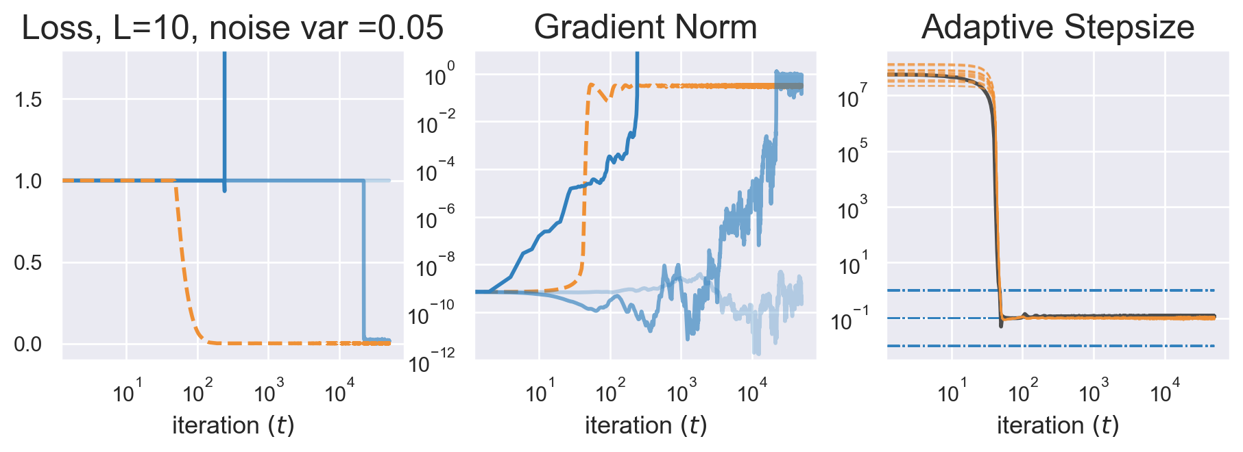
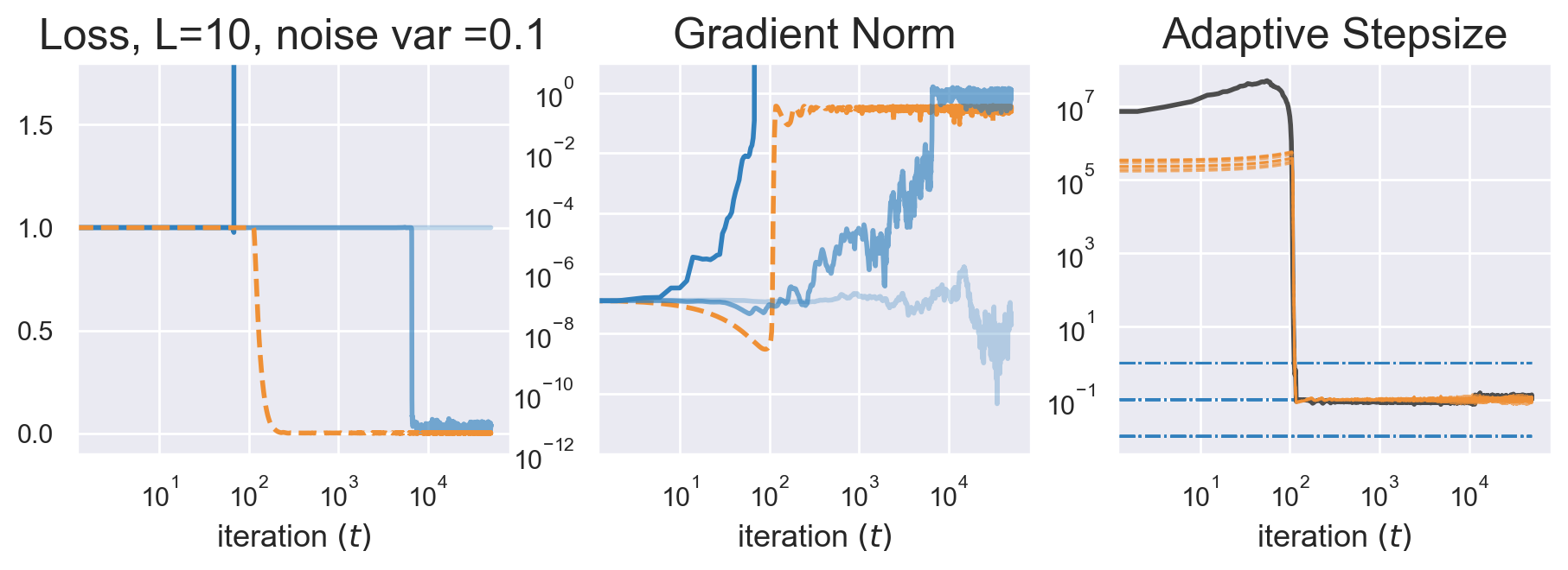
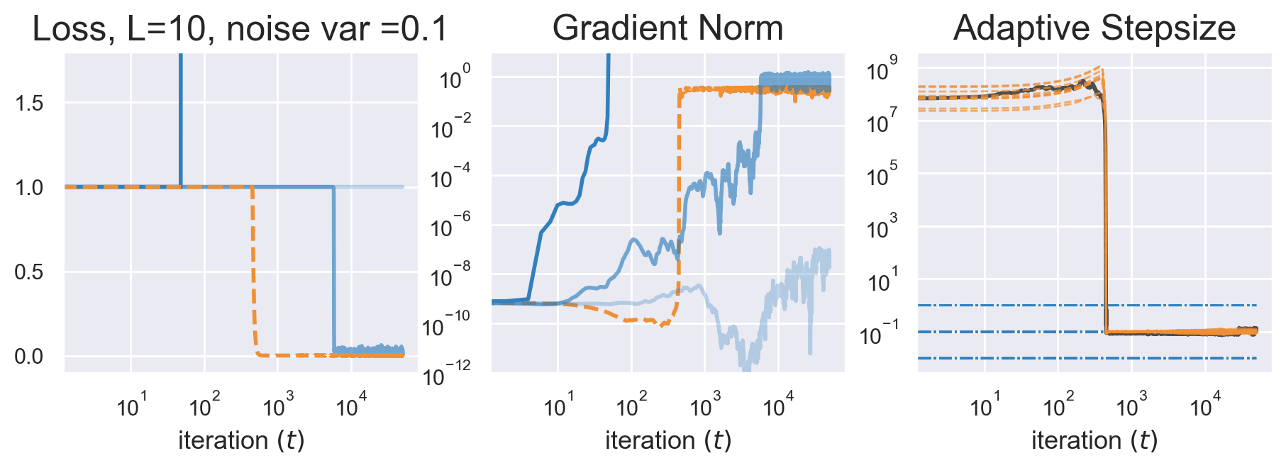
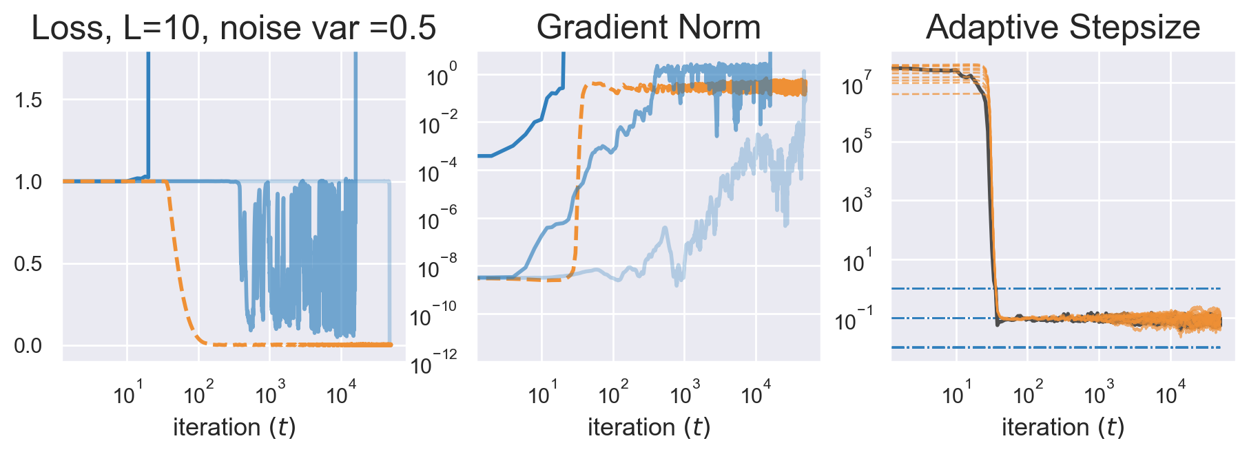
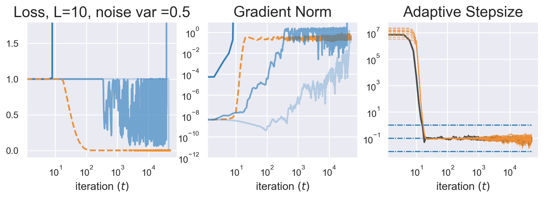
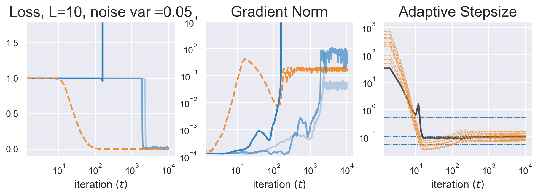
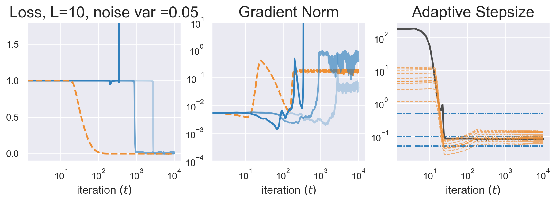
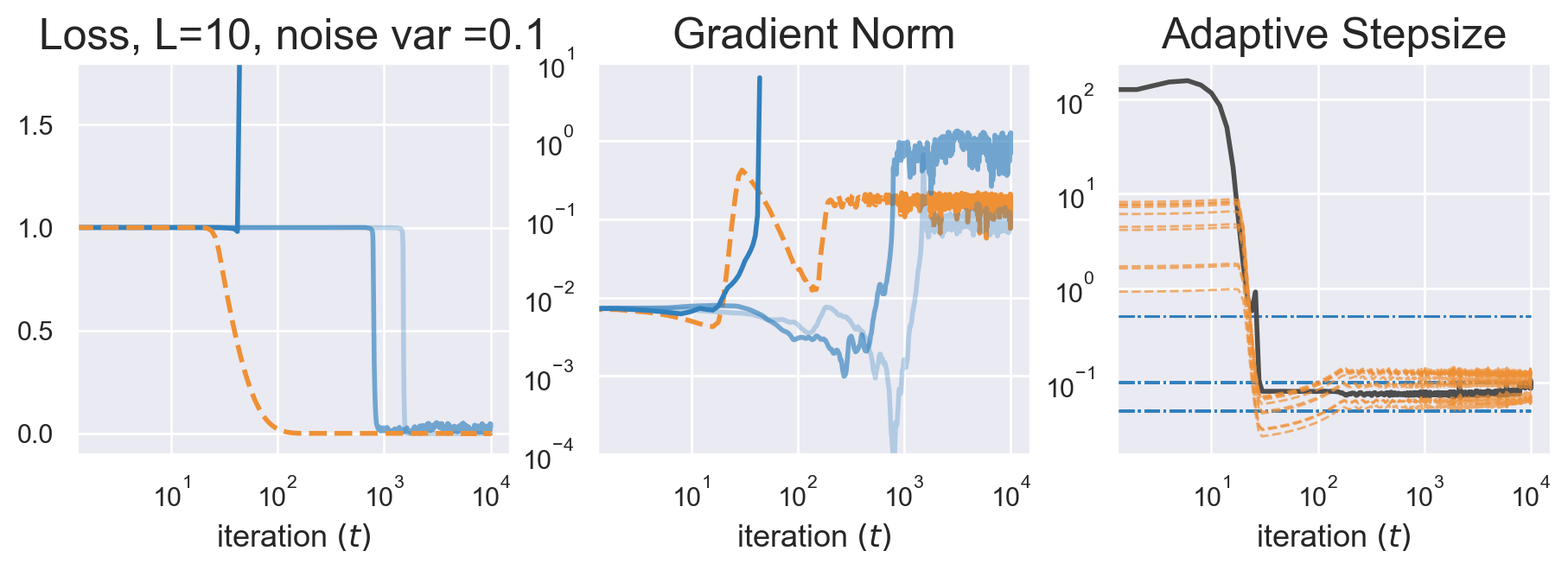
While it is known that the inherent sampling noise of SGD is anisotropic and in many settings aligned with negative curvature (Daneshmand et al., 2018; Zhu et al., 2018; Li et al., 2020), the saddle escape time still depends inversely on the magnitude of the smallest eigenvalue (Daneshmand et al., 2018; Curtis & Robinson, 2019). As a result, similar to gradient flow on the chain, SGD is unable to train networks with vanishing gradients/curvature despite the presence of inherent noise (see Fig. 5 & 8). Another possibility is to directly add noise to the updates (Du et al., 2017, 2019). In Fig. 23-25, we provide evidence that noise can indeed accelerate GD on the chain, but it is still orders of magnitude slower than RMSprop, for any noise level and stable learning rate.

4 Vanishing in MLPs of arbitrary width

In analogy with Prop. 3, we first note (proof in App. B) the important fact that also in the general MLP case different population quantities cannot be jointly stabilized using standard i.i.d. initialization.

Proposition 8 (Forward pass statistics MLP).
Let κ=μ4/σ4𝜅subscript𝜇4subscript𝜎4\kappa=\mu_{4}/\sigma_{4} be the kurtosis (fourth standardized moment). Let p=1𝑝1p=1 in the linear case and p=1/2𝑝12p=1/2 in the ReLU case. Then we have 𝔼𝐖ϕk:1𝐀𝐱22𝔼superscriptsubscriptnormsubscriptsuperscript𝐖:𝑘1italic-ϕ𝐀𝐱22\displaystyle{\mathbb{E}}\|\mathbf{W}^{k:1}_{\phi}{\bf A}{\bf x}\|_{2}^{2} =(dσ2p)k𝔼𝐀𝐱22.absentsuperscript𝑑superscript𝜎2𝑝𝑘𝔼subscriptsuperscriptnorm𝐀𝐱22\displaystyle=(d\sigma^{2}p)^{k}{\mathbb{E}}\|{\bf A}{\bf x}\|^{2}_{2}. (4) (𝔼𝐖ϕk:1𝐳24𝔼𝐖ϕk:1𝐳44)matrix𝔼superscriptsubscriptnormsubscriptsuperscript𝐖:𝑘1italic-ϕ𝐳24𝔼superscriptsubscriptnormsubscriptsuperscript𝐖:𝑘1italic-ϕ𝐳44\displaystyle\begin{pmatrix}{\mathbb{E}}\|\mathbf{W}^{k:1}_{\phi}{\bf z}\|_{2}^{4}\\ {\mathbb{E}}\|\mathbf{W}^{k:1}_{\phi}{\bf z}\|_{4}^{4}\end{pmatrix} =(p2dσ4)k𝐐k(𝔼𝐀𝐱24𝔼𝐀𝐱44),𝐐:=(d+2κ3+(1p)(d+2)p3κ3pp).formulae-sequenceabsentsuperscriptsuperscript𝑝2𝑑superscript𝜎4𝑘superscript𝐐𝑘matrix𝔼superscriptsubscriptnorm𝐀𝐱24𝔼superscriptsubscriptnorm𝐀𝐱44assign𝐐matrix𝑑2𝜅31𝑝𝑑2𝑝3𝜅3𝑝𝑝\displaystyle=\left(p^{2}d\sigma^{4}\right)^{k}{\bf Q}^{k}\begin{pmatrix}{\mathbb{E}}\|{\bf A}{\bf x}\|_{2}^{4}\\ {\mathbb{E}}\|{\bf A}{\bf x}\|_{4}^{4}\end{pmatrix},\quad{\bf Q}:=\begin{pmatrix}d+2&\frac{\kappa-3+(1-p)(d+2)}{p}\\ 3&\frac{\kappa-3p}{p}\end{pmatrix}. (5)

For deep linear nets of arbitrary width d𝑑d and Gaussian initialization (κ=3𝜅3\kappa=3) the above simplifies to

𝔼𝐖L:1𝐀𝐱22=(dσ2)L𝔼𝐀𝐱22and𝔼𝐖L:1𝐀𝐱24=(dσ4)L(d+2)L𝔼𝐀𝐱24.formulae-sequence𝔼superscriptsubscriptnormsuperscript𝐖:𝐿1𝐀𝐱22superscript𝑑superscript𝜎2𝐿𝔼subscriptsuperscriptnorm𝐀𝐱22and𝔼superscriptsubscriptnormsuperscript𝐖:𝐿1𝐀𝐱24superscript𝑑superscript𝜎4𝐿superscript𝑑2𝐿𝔼subscriptsuperscriptnorm𝐀𝐱42{\mathbb{E}}\|\mathbf{W}^{L:1}{\bf A}{\bf x}\|_{2}^{2}=(d\sigma^{2})^{L}{\mathbb{E}}\|{\bf A}{\bf x}\|^{2}_{2}\quad\text{and}\quad{\mathbb{E}}\|\mathbf{W}^{L:1}{\bf A}{\bf x}\|_{2}^{4}=\left(d\sigma^{4}\right)^{L}\left(d+2\right)^{L}{\mathbb{E}}\|{\bf A}{\bf x}\|^{4}_{2}. (6)

Hence, as for the neural chain (see Prop. 2), picking the Xavier initialization σ2=1dsuperscript𝜎21𝑑\sigma^{2}=\tfrac{1}{d} stabilizes 𝔼𝐖L:1𝐀𝐱22𝔼superscriptsubscriptnormsuperscript𝐖:𝐿1𝐀𝐱22{\mathbb{E}}\|\mathbf{W}^{L:1}{\bf A}{\bf x}\|_{2}^{2}, but 𝔼𝐖L:1𝐀𝐱24=(d+2d)L𝔼𝐀𝐱24𝔼superscriptsubscriptnormsuperscript𝐖:𝐿1𝐀𝐱24superscript𝑑2𝑑𝐿𝔼superscriptsubscriptnorm𝐀𝐱24{\mathbb{E}}\|\mathbf{W}^{L:1}{\bf A}{\bf x}\|_{2}^{4}=\left(\frac{d+2}{d}\right)^{L}{\mathbb{E}}\|{\bf A}{\bf x}\|_{2}^{4} explodes unless d𝑑d grows faster than L𝐿L. This points to an important shortcoming of the initialization proposed in Glorot & Bengio (2010) & He et al. (2015), which — as we note next — is only guaranteed to prevent vanishing gradients and curvature in networks that are wider than deep. The next result is verified in Fig. 20 in the appendix.

Theorem 9.
The initialization in Glorot & Bengio (2010) & He et al. (2015) is guaranteed to stabilize both the mean and the median of the squared forward pass norm for d=𝒪(L)𝑑𝒪𝐿d=\mathcal{O}(L).
Proof.

We carry out the proof for the Gaussian linear case, but the other settings are conceptually equivalent. First, in the case σ2=1/dsuperscript𝜎21𝑑\sigma^{2}=1/d, we have

Var𝐖L:1𝐀𝐱22=𝔼𝐖L:1𝐀𝐱24(𝔼𝐖L:1𝐀𝐱22)2=Eq.(6)(d+2d)L1.Varsuperscriptsubscriptnormsuperscript𝐖:𝐿1𝐀𝐱22𝔼superscriptsubscriptnormsuperscript𝐖:𝐿1𝐀𝐱24superscript𝔼superscriptsubscriptnormsuperscript𝐖:𝐿1𝐀𝐱222formulae-sequence𝐸𝑞italic-(6italic-)superscript𝑑2𝑑𝐿1\textrm{Var}\|\mathbf{W}^{L:1}{\bf A}{\bf x}\|_{2}^{2}={\mathbb{E}}\|\mathbf{W}^{L:1}{\bf A}{\bf x}\|_{2}^{4}-\left({\mathbb{E}}\|\mathbf{W}^{L:1}{\bf A}{\bf x}\|_{2}^{2}\right)^{2}\overset{Eq.~{}\eqref{eq:moments_wide}}{=}\left(\frac{d+2}{d}\right)^{L}-1. (7)

By Mallows inequality (Mallows & Richter, 1969), the square root of this quantity bounds |median(𝐖L:1𝐀𝐱22)𝔼𝐖L:1𝐀𝐱22|mediansuperscriptsubscriptnormsuperscript𝐖:𝐿1𝐀𝐱22𝔼superscriptsubscriptnormsuperscript𝐖:𝐿1𝐀𝐱22\left|\text{median}\left(\|\mathbf{W}^{L:1}{\bf A}{\bf x}\|_{2}^{2}\right)-{\mathbb{E}}\|\mathbf{W}^{L:1}{\bf A}{\bf x}\|_{2}^{2}\right|. If we want to guarantee a non-vanishing median, say in [1α,1+α]1𝛼1𝛼[1-\alpha,1+\alpha], for 1>α>01𝛼01>\alpha>0, we need to have d𝑑d s.t. (d+2d)L1α2superscript𝑑2𝑑𝐿1superscript𝛼2\left(\frac{d+2}{d}\right)^{L}-1\leq\alpha^{2} which implies d2(α2+1)1L1𝑑2superscriptsuperscript𝛼211𝐿1d\geq\frac{2}{(\alpha^{2}+1)^{\frac{1}{L}}-1}. For L𝐿L\to\infty we have (α2+1)1L=1+ln(α2+1)/L+𝒪(1/L2)superscriptsuperscript𝛼211𝐿1superscript𝛼21𝐿𝒪1superscript𝐿2(\alpha^{2}+1)^{\frac{1}{L}}=1+\ln(\alpha^{2}+1)/L+\mathcal{O}(1/L^{2}), thus we conclude d𝒪(L)𝑑𝒪𝐿d\geq\mathcal{O}(L). ∎

Before discussing the regime dLmuch-less-than𝑑𝐿d\ll L, we first consolidate our core claim about vanishing curvature by generalizing the results of (Glorot & Bengio, 2010; He et al., 2015) to second-order derivatives.

Theorem 10 (Gradient and Hessian in expectation).
Under Assumption 1, the expected norm of any Hessian diagonal block 𝔼[2(𝐖)𝐖k𝐖kF]𝔼delimited-[]subscriptnormsuperscript2𝐖subscript𝐖𝑘subscript𝐖𝑘𝐹{\mathbb{E}}[\|\tfrac{\partial^{2}{\mathcal{L}}({\bf W})}{\partial{\bf W}_{k}\partial{\bf W}_{k}}\|_{F}] in linear networks scales as 𝒪((dσ2)L)𝒪superscript𝑑superscript𝜎2𝐿\mathcal{O}\left((d\sigma^{2})^{L}\right), while off-diagonal blocks 𝔼[2(𝐖)𝐖k𝐖F]𝔼delimited-[]subscriptnormsuperscript2𝐖subscript𝐖𝑘subscript𝐖𝐹{\mathbb{E}}[\|\tfrac{\partial^{2}{\mathcal{L}}({\bf W})}{\partial{\bf W}_{k}\partial{\bf W}_{\ell}}\|_{F}] as well as the gradient 𝔼[(𝐖)𝐖kF]𝔼delimited-[]subscriptnorm𝐖subscript𝐖𝑘𝐹{\mathbb{E}}[\|\tfrac{\partial{\mathcal{L}}({\bf W})}{\partial{\bf W}_{k}}\|_{F}] scale as 𝒪((dσ2)L2)𝒪superscript𝑑superscript𝜎2𝐿2\mathcal{O}\left((d\sigma^{2})^{\frac{L}{2}}\right). In ReLU networks the scaling amounts to 𝒪((d2σ2)L)𝒪superscript𝑑2superscript𝜎2𝐿\mathcal{O}\left(\left(\frac{d}{2}\sigma^{2}\right)^{L}\right) and 𝒪((d2σ2)L2)𝒪superscript𝑑2superscript𝜎2𝐿2\mathcal{O}\left(\left(\frac{d}{2}\sigma^{2}\right)^{\frac{L}{2}}\right) respectively.

This result is (to the best of our knowledge) the first to study the effects of depth on second-order derivatives at random initialization. Its proof, which mainly builds upon Prop. 8, can be found in App. B. A simple application of Gershgorin’s theorem yields the following bound on the eigenvalues.
Corollary 11.
Under Assumption 1, the expected magnitude of the largest eigenvalue λmaxsubscript𝜆\lambda_{\max} is upper bound as 𝔼[|λmaxlinear|]Ld𝒪((dσ2)L2)𝔼delimited-[]subscriptsuperscript𝜆linear𝐿𝑑𝒪superscript𝑑superscript𝜎2𝐿2{\mathbb{E}}[|\lambda^{\text{linear}}_{\max}|]\leq Ld\cdot\mathcal{O}\left((d\sigma^{2})^{\frac{L}{2}}\right) and 𝔼[|λmaxReLU|]Ld𝒪((d2σ2)L2)𝔼delimited-[]subscriptsuperscript𝜆ReLU𝐿𝑑𝒪superscript𝑑2superscript𝜎2𝐿2{\mathbb{E}}[|\lambda^{\text{ReLU}}_{\max}|]\leq Ld\cdot\mathcal{O}\left((\frac{d}{2}\sigma^{2})^{\frac{L}{2}}\right) respectively.
Refer to caption
Refer to caption
Refer to caption
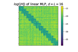
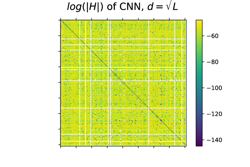
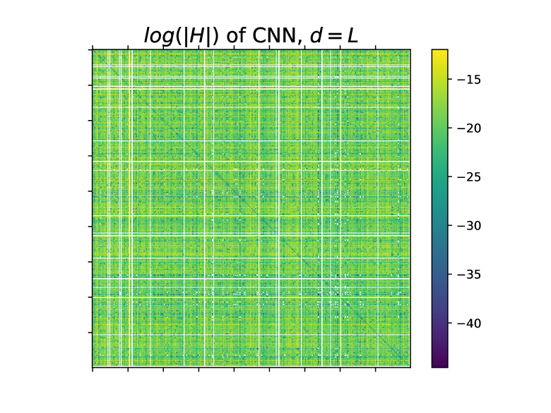
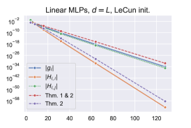
Figure 4: Left: Vanishing gradient and Hessian for deep linear MLPs with LeCun init. x-axis depicts depth and width. Middle/Right: log abs. Hessian entries and eigenvalues at random init. (see ReLU MLP in Fig. 1)

Consequences for traditional LeCun init.

The above results point to an important consequence of the standard way of initialization prior to (Glorot & Bengio, 2010). When choosing σ2=13dsuperscript𝜎213𝑑\sigma^{2}=\tfrac{1}{3d} as in LeCun init. (LeCun et al., 1998), gradient- and Hessian off-diagonal norms in (e.g.) linear nets vanish as 𝒪((13)L/2)𝒪superscript13𝐿2\mathcal{O}((\tfrac{1}{3})^{L/2}) and Hessian diagonal blocks vanish even faster, namely at 𝒪((13)L)𝒪superscript13𝐿\mathcal{O}((\tfrac{1}{3})^{L}) (Fig. 4 & 13). This points to an important fact about the eigenspectrum of the Hessian. Since, 𝔼2(𝐖)F𝔼subscriptnormsuperscript2𝐖𝐹{\mathbb{E}}\|\nabla^{2}{\mathcal{L}}({\bf W})\|_{F} scales as (dσ2)L2superscript𝑑superscript𝜎2𝐿2(d\sigma^{2})^{\frac{L}{2}} by Thm. 10, one of the Ld2𝐿superscript𝑑2Ld^{2} eigenvales must have a magnitude (dσ2)L2superscript𝑑superscript𝜎2𝐿2(d\sigma^{2})^{\frac{L}{2}} in expectation. Yet, the fast diagonal vanishing lets the trace scale as (dσ2)Lsuperscript𝑑superscript𝜎2𝐿(d\sigma^{2})^{L}. As a result, the sum of the eigenvalues is exponentially smaller than the maximum eigenvalue and hence there must be eigenvalues of opposite sign (see e.g. Fig. 4). In summary, as in neural chains, optimizers are initialized in a flat plateau with almost no gradient signal and both positive as well as negative, but very small eigenvalues.
Refer to caption
Refer to caption
Refer to caption
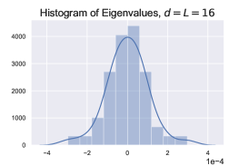
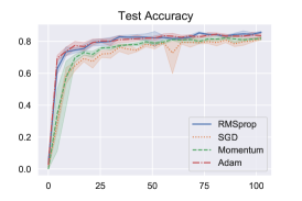
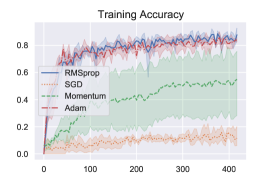
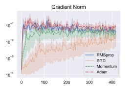
Figure 5: Fashion-MNIST on a narrow (32 hidden units) 128 layer ReLU MLP with He init. Mean and 95%percent\% CI of 10 random seeds. See App. A.1 for hyperparameters and Fig. 10 for test accuracy. Note that RMSProp successfully trains despite the fact that both gradients and curvature vanished (also compare Fig. 1). Yet, as can be deduced from how gradient norms evolve over time, SGD struggles to escape the flat plateau which is not surprising given that the negative eigenvalues are very small (compare Fig. 9 for a wide version of this network.)

Consequences for Xavier and He init.

Thm. 9 & 10 provide simple theoretical grounding for the benefits of increasing width in random neural networks.444(Hanin & Nica, 2019; Allen-Zhu et al., 2019) come to similar conclusions albeit with more complex analysis. However, they also point out an important limitation in the analysis and applicability of (Glorot & Bengio, 2010; He et al., 2015). What happens in cases where width scales sub-linearly with depth remains open for theoretical analysis.

Our study on the neural chain (Thm. 6) along with Thm. 9 suggests that no initialization variance σ2superscript𝜎2\sigma^{2} is capable of stabilizing the full distribution of all of activation-, gradient- and the Hessian norm when the width is small. Yet, characterizing the almost sure behaviour of the gradient and Hessian for networks with d>1𝑑1d>1 is intricate since paths in fully connected networks overlap, such that one cannot treat them as a set of independent products of random variables, which would allow a straight forward generalization of Thm. 6 using Berry-Esseen inequality (Berry, 1941). Similarly, deriving the distribution of the forward pass is very challenging. In fact, already in the scalar case (neural chain), product distributions for both uniform (Dettmann & Georgiou, 2009) and Gaussian initialization become very complex (Springer & Thompson, 1970). We thus retreat to empirical simulations, but stress the fact that these are informative because they are undertaken in a controlled setting, where the only source of randomness (weight initialization) is well controlled by running multiple seeds.

Our empirical results highlight that σ2=1dsuperscript𝜎21𝑑\sigma^{2}=\frac{1}{d} is indeed not an optimal choice for narrow networks. Indeed, as can be seen in Fig.1, gradients and curvature vanish in narrow but stay stable in wide ReLU MLPs with He init. The same happens in linear networks with Xavier init (Fig. 15). Again, we find both negative and positive eigenvalues at initialization (Fig. 12). Interestingly, Fig. 20 depicts that the optimal initialization variance σ2superscript𝜎2\sigma^{2} is a function g(d,L)𝑔𝑑𝐿g(d,L) of the width to depth ratio. This function is highly non-trivial as it depends not only on the number of paths but also on their mutual overlap. In the following section, we show that these considerations extend to convolutional neural networks.

5 Vanishing in convolutional networks

Next, we discuss the effects of increasing width in convolutional architectures. For simplicity, we consider an image to image learning setting with images of resolution r×r𝑟𝑟r\times r, using fully convolutional networks (FCNs) with k×k𝑘𝑘k\times k filters (where k𝑘k is odd), c𝑐c channels in each layer and a padding of (k1)/2𝑘12(k-1)/2 (such that the resolution does not change over depth). We first note that width is not as straight-forward to define in CNNs as it is in MLPs. In Sec. 3, we argue that it is the number of paths leading to an output neuron (as well as their level of overlap) that determines its activation magnitude. While there are |Γ|=dLΓsuperscript𝑑𝐿|\Gamma|=d^{L} paths in MLPs, the FCN architecture yields |Γ|=(k2c)LΓsuperscriptsuperscript𝑘2𝑐𝐿|\Gamma|=(k^{2}c)^{L} (assuming non-zero padding). Consequently, we define the effective network width as d:=k2cassign𝑑superscript𝑘2𝑐d:=k^{2}c. Obviously, there are then two ways to increase width, namely via the filter size k𝑘k and the number of channels c𝑐c. As in prior theoretical (Arora et al., 2019) and practical works (Zagoruyko & Komodakis, 2016), we focus on the latter option.

Empirical findings.

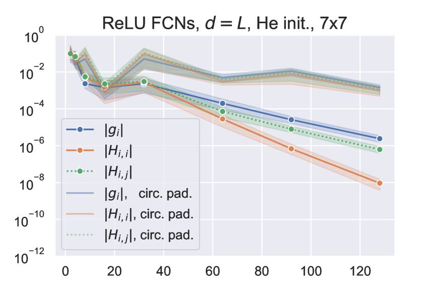
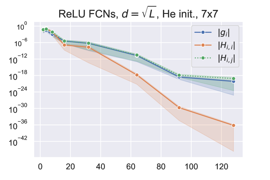
We first consider the above introduced image to image learning setting with CIFAR-10 images as inputs and targets, once at the original 32×32323232\times 32 resolution and once downsized to 7×7777\times 7. We fix the kernel size k:=3assign𝑘3k:=3 and increase both the number of layers and channels. As can be seen in Fig.6, gradients/curvature vanish when depth grows faster than width and again the Hessian diagonal decreases fastest (top). Due to weight sharing, the effect is more pronounced as in MLPs (see App. D for discussion). When width grows linearly in depth (bottom), however, the beneficial effect is reduced when operating at small resolutions, where the pixel to padding ratio goes down such that zero-padding has a detrimental effect on the gradient/Hessian magnitude over depth. As indicated on the bottom right, this effect can be circumvented by opting for non-zero padding (circular in this case).
Refer to caption

depth

Refer to caption

depth

Figure 6: Effect of width in CNNs: Gradient/curvature on FCNs over depth. Plots has different scales. Mean and 95% CI of 15 runs. While increasing width helps for large resolution (see Fig. 16), for small resolutions such as 7x7 (above) vanishing occurs even when width scales as 𝒪(L)𝒪𝐿\mathcal{O}(L) (albeit at slower rate (see y-axis)). Interestingly, replacing zero- with circular padding mitigates this effect.

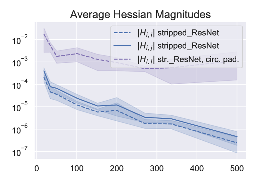
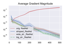
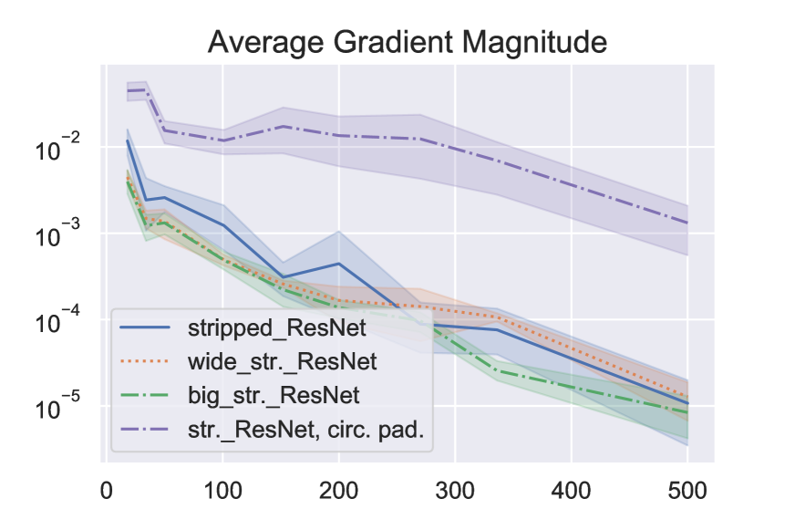
At first, 7×7777\times 7 may seem unrealistically small but we remark that even when training on 224×224224224224\times 224 ImageNet inputs, the last block of layers in ResNets indeed operates exactly at this scale (He et al., 2016a). Consequently, vanishing also occurs in ResNet-type architectures, despite their large number of channels (Fig. 7). Here, similarly to Yao et al. (2019), we feed images through ResNet architectures stripped of both batch normalization and residual connections, which we term stripped_ResNets. Interestingly, neither increasing the number of channels by two as in (Zagoruyko & Komodakis, 2016) (wide_stripped_ResNets) nor increasing the filter sizes from 1×1111\times 1 to 3×3333\times 3 and from 3×3333\times 3 to 5×5555\times 5 (big_stripped_ResNets) prevents gradient/curvature vanishing in deep stripped ResNets.
Refer to caption

depth

Refer to caption

depth

Figure 7: Left: Gradient in stripped_ResNets with He init. on CIFAR-10. Increasing number of channels (wide_stripped_ResNet) and kernel size (big_stripped_ResNet) does not help. Yet, as in Fig. 6, circular padding slows the effect down. Right: Average Hessian entry magnitudes in stripped ResNet (wide and big not computed due to memory limitations). Mean and 95% CI of 10 runs.

Architectural improvements

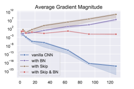
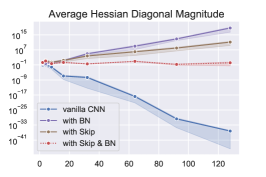
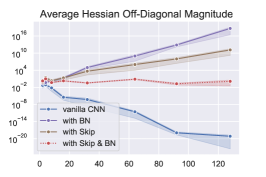
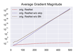
As mentioned in the introduction, convolutional networks of depth 500 and more are not unheard-of. In fact, He et al. (2016b) find that even going up to ResNet-1001 can improve test performance. Compared to the stripped_ResNets considered above, their architecture includes batch normalization and residual connections. Understanding the inner working of these components is an active area of research (e.g. (Hardt & Ma, 2016; Bjorck et al., 2018; Kohler et al., 2019; Yao et al., 2019; Zhang et al., 2019b)). Most related to our cases, Labatie (2019) suggests that only the combination of the two is effective in stabilizing information flow in the large depth limit, which is line with our finding that ResNets suffer from exploding gradients when taking either one of BN or residual connections out (Fig. 19).555Figure 17 & 18 confirm this for MLPs and FCNs. See also (Yang et al., 2019) and (Zhang et al., 2019a)

Algorithmic improvements.

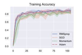
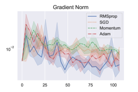
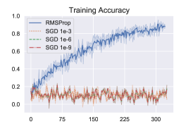
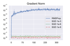
An obvious alternative is to generate robustness towards gradient/curvature vanishing directly in the training algorithm. As discussed in Section 3, adaptive gradient methods (that were introduced about five years prior to batch normalization) are indeed able to escape flat initialization plateaus quickly. As a result, RMSprop can train a 500 layer stripped_ResNet without any normalization, skip-connections or learning-rate scheduling (Fig. 8).
Refer to caption
Refer to caption
Refer to caption
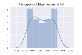
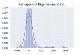
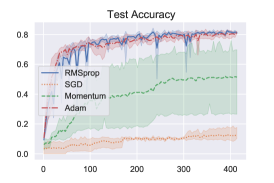
Figure 8: CIFAR-10 on a 500 layer stripped_ResNet with He init. Accuracy and gradient norm over epochs as well as eigenvalue histogram at initialization. Mean and 95%percent\% CI of 10 random seeds. See Appendix A.1 for hyperparameters and Figure 10 for test accuracy

6 Conclusion and outlook

Despite its long standing history, the phenomenon of vanishing and exploding gradients still lacks a comprehensive explanation. In this retrospective work we extended the current state of knowledge by: (i) showing that vanishing gradient co-occur with vanishing curvature, which clarifies the detrimental effect of depth on standard gradient descent at random initialization; (ii) examining when and why vanishing gradients occur in the first place. In this regard, we highlighted the role of effective width as well as the importance of combining Batch Normalization with residual connections; (iii) pointing to a remarkable curvature adaption property of adaptive gradients methods which allows them to train very deep networks despite the above mentioned issues.

Looking ahead, we regard investigations into quantifying the optimal variance for narrow MLPs as well as for un-normalized convnets an interesting follow-up. Furhtermore, clarifying the interplay of initialization and activation functions (Fig. 18) poses yet another interesting question. On a different route, we consider moving away from i.i.d. initialization and instead developing balanced initialization schemes that couple layers but preserve randomness a promising direction for designing simple deep neural network architectures that train and generalize well with gradient based methods.

References

  • Allen-Zhu et al. (2019) Allen-Zhu, Z., Li, Y., and Song, Z. A convergence theory for deep learning via over-parameterization. In International Conference on Machine Learning, pp. 242–252. PMLR, 2019.
  • Arjevani et al. (2019) Arjevani, Y., Carmon, Y., Duchi, J. C., Foster, D. J., Srebro, N., and Woodworth, B. Lower bounds for non-convex stochastic optimization. arXiv preprint:1912.02365, 2019.
  • Arora et al. (2019) Arora, S., Du, S. S., Hu, W., Li, Z., Salakhutdinov, R. R., and Wang, R. On exact computation with an infinitely wide neural net. In Advances in Neural Information Processing Systems, pp. 8141–8150, 2019.
  • Balles & Hennig (2018) Balles, L. and Hennig, P. Dissecting Adam: The sign, magnitude and variance of stochastic gradients. In International Conference on Machine Learning, pp. 404–413. PMLR, 2018.
  • Bengio et al. (1994) Bengio, Y., Simard, P., and Frasconi, P. Learning long-term dependencies with gradient descent is difficult. IEEE transactions on neural networks, 5(2):157–166, 1994.
  • Berry (1941) Berry, A. C. The accuracy of the Gaussian approximation to the sum of independent variates. Transactions of the American Mathematical Society, 49(1):122–136, 1941.
  • Bjorck et al. (2018) Bjorck, J., Gomes, C., Selman, B., and Weinberger, K. Q. Understanding batch normalization. arXiv preprint:1806.02375, 2018.
  • Brock et al. (2018) Brock, A., Donahue, J., and Simonyan, K. Large scale gan training for high fidelity natural image synthesis. In International Conference on Learning Representations, 2018.
  • Brown et al. (2020) Brown, T. B., Mann, B., Ryder, N., Subbiah, M., Kaplan, J., Dhariwal, P., Neelakantan, A., Shyam, P., Sastry, G., Askell, A., et al. Language models are few-shot learners. arXiv preprint:2005.14165, 2020.
  • Chen et al. (2020) Chen, J., Zhou, D., Tang, Y., Yang, Z., Cao, Y., and Gu, Q. Closing the generalization gap of adaptive gradient methods in training deep neural networks. In IJCAI, 2020.
  • Choi (1994) Choi, K. P. On the medians of gamma distributions and an equation of Ramanujan. Proceedings of the American Mathematical Society, 121(1):245–251, 1994.
  • Curtis & Robinson (2019) Curtis, F. E. and Robinson, D. P. Exploiting negative curvature in deterministic and stochastic optimization. Mathematical Programming, 176(1-2):69–94, 2019.
  • Cutkosky & Orabona (2019) Cutkosky, A. and Orabona, F. Momentum-based variance reduction in non-convex sgd. Advances in neural information processing systems, 32, 2019.
  • Daneshmand et al. (2018) Daneshmand, H., Kohler, J., Lucchi, A., and Hofmann, T. Escaping saddles with stochastic gradients. arXiv preprint:1803.05999, 2018.
  • Daneshmand et al. (2020) Daneshmand, H., Kohler, J., Bach, F., Hofmann, T., and Lucchi, A. Batch normalization provably avoids ranks collapse for randomly initialised deep networks. Advances in Neural Information Processing Systems, 33, 2020.
  • Dauphin et al. (2015) Dauphin, Y., de Vries, H., and Bengio, Y. Equilibrated adaptive learning rates for non-convex optimization. In NIPS, 2015.
  • De & Smith (2020) De, S. and Smith, S. Batch normalization biases residual blocks towards the identity function in deep networks. Advances in Neural Information Processing Systems, 33, 2020.
  • Défossez et al. (2020) Défossez, A., Bottou, L., Bach, F., and Usunier, N. On the convergence of Adam and Adagrad. arXiv preprint:2003.02395, 2020.
  • Dettmann & Georgiou (2009) Dettmann, C. P. and Georgiou, O. Product of n𝑛n independent uniform random variables. Statistics & probability letters, 79(24):2501–2503, 2009.
  • Devroye (2006) Devroye, L. Nonuniform random variate generation. Handbooks in operations research and management science, 13:83–121, 2006.
  • Du et al. (2019) Du, S., Lee, J., Li, H., Wang, L., and Zhai, X. Gradient descent finds global minima of deep neural networks. In International Conference on Machine Learning, pp. 1675–1685. PMLR, 2019.
  • Du et al. (2017) Du, S. S., Jin, C., Lee, J. D., Jordan, M. I., Singh, A., and Poczos, B. Gradient descent can take exponential time to escape saddle points. In Advances in neural information processing systems, pp. 1067–1077, 2017.
  • Duchi et al. (2011) Duchi, J., Hazan, E., and Singer, Y. Adaptive subgradient methods for online learning and stochastic optimization. Journal of machine learning research, 12(7), 2011.
  • Fang et al. (2019) Fang, C., Lin, Z., and Zhang, T. Sharp analysis for nonconvex sgd escaping from saddle points. arXiv preprint:1902.00247, 2019.
  • Gemp & McWilliams (2019) Gemp, I. and McWilliams, B. The unreasonable effectiveness of Adam on cycles. NeurIPS Workshop on Bridging Game Theory and Deep Learning, 2019.
  • Gershgorin (1931) Gershgorin, S. On the location of eigenvalues of a matrix. Izv. Akad. Nauk SSSR, ser. Fiz. Mat. v6, 749, 1931.
  • Ghadimi & Lan (2013) Ghadimi, S. and Lan, G. Stochastic first-and zeroth-order methods for nonconvex stochastic programming. SIAM Journal on Optimization, 23(4):2341–2368, 2013.
  • Glorot & Bengio (2010) Glorot, X. and Bengio, Y. Understanding the difficulty of training deep feedforward neural networks. In Proceedings of the thirteenth international conference on artificial intelligence and statistics, pp.  249–256, 2010.
  • Goodfellow et al. (2014) Goodfellow, I. J., Pouget-Abadie, J., Mirza, M., Xu, B., Warde-Farley, D., Ozair, S., Courville, A. C., and Bengio, Y. Generative adversarial nets. In NIPS, 2014.
  • Hanin & Nica (2019) Hanin, B. and Nica, M. Products of many large random matrices and gradients in deep neural networks. Communications in Mathematical Physics, pp.  1–36, 2019.
  • Hardt & Ma (2016) Hardt, M. and Ma, T. Identity matters in deep learning. arXiv preprint:1611.04231, 2016.
  • He et al. (2015) He, K., Zhang, X., Ren, S., and Sun, J. Delving deep into rectifiers: Surpassing human-level performance on imagenet classification. In Proceedings of the IEEE international conference on computer vision, pp.  1026–1034, 2015.
  • He et al. (2016a) He, K., Zhang, X., Ren, S., and Sun, J. Deep residual learning for image recognition. In Proceedings of the IEEE conference on computer vision and pattern recognition, pp.  770–778, 2016a.
  • He et al. (2016b) He, K., Zhang, X., Ren, S., and Sun, J. Identity mappings in deep residual networks. In European conference on computer vision, pp.  630–645. Springer, 2016b.
  • Hochreiter (1991) Hochreiter, S. Untersuchungen zu dynamischen neuronalen netzen. Diploma, Technische Universität München, 91(1), 1991.
  • Hochreiter & Schmidhuber (1997) Hochreiter, S. and Schmidhuber, J. Long short-term memory. Neural computation, 9(8):1735–1780, 1997.
  • Ioffe & Szegedy (2015) Ioffe, S. and Szegedy, C. Batch normalization: Accelerating deep network training by reducing internal covariate shift. arXiv preprint:1502.03167, 2015.
  • Karras et al. (2020a) Karras, T., Aittala, M., Hellsten, J., Laine, S., Lehtinen, J., and Aila, T. Training generative adversarial networks with limited data. arXiv preprint:2006.06676, 2020a.
  • Karras et al. (2020b) Karras, T., Laine, S., Aittala, M., Hellsten, J., Lehtinen, J., and Aila, T. Analyzing and improving the image quality of stylegan. In Proceedings of the IEEE/CVF Conference on Computer Vision and Pattern Recognition, pp.  8110–8119, 2020b.
  • Kingma & Ba (2014) Kingma, D. P. and Ba, J. Adam: A method for stochastic optimization. arXiv preprint:1412.6980, 2014.
  • Kohler et al. (2019) Kohler, J., Daneshmand, H., Lucchi, A., Hofmann, T., Zhou, M., and Neymeyr, K. Exponential convergence rates for batch normalization: The power of length-direction decoupling in non-convex optimization. In The 22nd International Conference on Artificial Intelligence and Statistics, pp.  806–815. PMLR, 2019.
  • Krizhevsky (2009) Krizhevsky, A. Learning multiple layers of features from tiny images. cs.toronto.edu, 2009.
  • Kunstner et al. (2019) Kunstner, F., Hennig, P., and Balles, L. Limitations of the empirical Fisher approximation for natural gradient descent. In Advances in Neural Information Processing Systems, pp. 4156–4167, 2019.
  • Labatie (2019) Labatie, A. Characterizing well-behaved vs. pathological deep neural networks. In International Conference on Machine Learning, pp. 3611–3621. PMLR, 2019.
  • LeCun et al. (1998) LeCun, Y. A., Bottou, L., Orr, G. B., and Müller, K.-R. Efficient backprop. In Neural networks: Tricks of the trade, pp.  9–48. Springer, 1998.
  • Li et al. (2020) Li, X., Gu, Q., Zhou, Y., Chen, T., and Banerjee, A. Hessian based analysis of sgd for deep nets: Dynamics and generalization. In Proceedings of the 2020 SIAM International Conference on Data Mining, pp.  190–198. SIAM, 2020.
  • Liu et al. (2019) Liu, L., Jiang, H., He, P., Chen, W., Liu, X., Gao, J., and Han, J. On the variance of the adaptive learning rate and beyond. arXiv preprint:1908.03265, 2019.
  • Loshchilov & Hutter (2017) Loshchilov, I. and Hutter, F. Decoupled weight decay regularization. arXiv preprint:1711.05101, 2017.
  • Mallows & Richter (1969) Mallows, C. L. and Richter, D. Inequalities of Chebyshev type involving conditional expectations. The Annals of Mathematical Statistics, 40(6):1922–1932, 1969.
  • Martens (2020) Martens, J. New insights and perspectives on the natural gradient method. Journal of Machine Learning Research, 21:1–76, 2020.
  • Nesterov et al. (2018) Nesterov, Y. et al. Lectures on convex optimization, volume 137. Springer, 2018.
  • Nocedal & Wright (2006) Nocedal, J. and Wright, S. Numerical optimization. Springer Science & Business Media, 2006.
  • Park et al. (2019) Park, T., Liu, M.-Y., Wang, T.-C., and Zhu, J.-Y. Semantic image synthesis with spatially-adaptive normalization. In Proceedings of the IEEE/CVF Conference on Computer Vision and Pattern Recognition, pp.  2337–2346, 2019.
  • Pascanu et al. (2013) Pascanu, R., Mikolov, T., and Bengio, Y. On the difficulty of training recurrent neural networks. In International conference on machine learning, pp. 1310–1318, 2013.
  • Paszke et al. (2019) Paszke, A., Gross, S., Massa, F., Lerer, A., Bradbury, J., Chanan, G., Killeen, T., Lin, Z., Gimelshein, N., Antiga, L., et al. Pytorch: An imperative style, high-performance deep learning library. In Advances in neural information processing systems, pp. 8026–8037, 2019.
  • Pennington et al. (2018) Pennington, J., Schoenholz, S., and Ganguli, S. The emergence of spectral universality in deep networks. In International Conference on Artificial Intelligence and Statistics, pp.  1924–1932, 2018.
  • Reddi et al. (2019) Reddi, S. J., Kale, S., and Kumar, S. On the convergence of Adam and beyond. arXiv preprint:1904.09237, 2019.
  • Saxe et al. (2013) Saxe, A. M., McClelland, J. L., and Ganguli, S. Exact solutions to the nonlinear dynamics of learning in deep linear neural networks. arXiv preprint:1312.6120, 2013.
  • Schoenholz et al. (2016) Schoenholz, S. S., Gilmer, J., Ganguli, S., and Sohl-Dickstein, J. Deep information propagation. arXiv preprint:1611.01232, 2016.
  • Springer & Thompson (1970) Springer, M. D. and Thompson, W. E. The distribution of products of beta, gamma and Gaussian random variables. SIAM Journal on Applied Mathematics, 18(4):721–737, 1970.
  • Staib et al. (2019) Staib, M., Reddi, S., Kale, S., Kumar, S., and Sra, S. Escaping saddle points with adaptive gradient methods. In International Conference on Machine Learning, pp. 5956–5965. PMLR, 2019.
  • Tan & Le (2019) Tan, M. and Le, Q. Efficientnet: Rethinking model scaling for convolutional neural networks. In International Conference on Machine Learning, pp. 6105–6114. PMLR, 2019.
  • Tan et al. (2019) Tan, M., Chen, B., Pang, R., Vasudevan, V., Sandler, M., Howard, A., and Le, Q. V. Mnasnet: Platform-aware neural architecture search for mobile. In Proceedings of the IEEE/CVF Conference on Computer Vision and Pattern Recognition, pp.  2820–2828, 2019.
  • Telgarsky (2016) Telgarsky, M. Benefits of depth in neural networks. arXiv preprint:1602.04485, 2016.
  • Temme (1996) Temme, N. M. Special functions: An introduction to the classical functions of mathematical physics. John Wiley & Sons, 1996.
  • Tieleman & Hinton (2012) Tieleman, T. and Hinton, G. Lecture 6.5-rmsprop: Divide the gradient by a running average of its recent magnitude. COURSERA: Neural networks for machine learning, 4(2):26–31, 2012.
  • Wilson et al. (2017) Wilson, A. C., Roelofs, R., Stern, M., Srebro, N., and Recht, B. The marginal value of adaptive gradient methods in machine learning. In Proceedings of the 31st International Conference on Neural Information Processing Systems, pp.  4151–4161, 2017.
  • Wolf et al. (2020) Wolf, T., Debut, L., Sanh, V., Chaumond, J., Delangue, C., Moi, A., Cistac, P., Rault, T., Louf, R., Funtowicz, M., Davison, J., Shleifer, S., von Platen, P., Ma, C., Jernite, Y., Plu, J., Xu, C., Scao, T. L., Gugger, S., Drame, M., Lhoest, Q., and Rush, A. M. Transformers: State-of-the-art natural language processing. In Proceedings of the 2020 Conference on Empirical Methods in Natural Language Processing: System Demonstrations, pp.  38–45, October 2020.
  • Xiao et al. (2017) Xiao, H., Rasul, K., and Vollgraf, R. Fashion-mnist: a novel image dataset for benchmarking machine learning algorithms. arXiv preprint:1708.07747, 2017.
  • Yang et al. (2019) Yang, G., Pennington, J., Rao, V., Sohl-Dickstein, J., and Schoenholz, S. S. A mean field theory of batch normalization. arXiv preprint:1902.08129, 2019.
  • Yao et al. (2019) Yao, Z., Gholami, A., Keutzer, K., and Mahoney, M. Pyhessian: Neural networks through the lens of the hessian. arXiv preprint:1912.07145, 2019.
  • Zagoruyko & Komodakis (2016) Zagoruyko, S. and Komodakis, N. Wide residual networks. arXiv preprint:1605.07146, 2016.
  • Zhang et al. (2019a) Zhang, H., Dauphin, Y. N., and Ma, T. Fixup initialization: Residual learning without normalization. arXiv preprint:1901.09321, 2019a.
  • Zhang et al. (2019b) Zhang, H., Yu, D., Yi, M., Chen, W., and Liu, T.-Y. Convergence theory of learning over-parameterized resnet: A full characterization. arXiv preprint:1903.07120, 2019b.
  • Zhang et al. (2019c) Zhang, J., He, T., Sra, S., and Jadbabaie, A. Why gradient clipping accelerates training: A theoretical justification for adaptivity. In International Conference on Learning Representations, 2019c.
  • Zhang et al. (2020) Zhang, J., Karimireddy, S. P., Veit, A., Kim, S., Reddi, S., Kumar, S., and Sra, S. Why are adaptive methods good for attention models? Advances in Neural Information Processing Systems, 33, 2020.
  • Zhu et al. (2018) Zhu, Z., Wu, J., Yu, B., Wu, L., and Ma, J. The anisotropic noise in stochastic gradient descent: Its behavior of escaping from minima and regularization effects, 2018.
  • Zhu et al. (2019) Zhu, Z., Wu, J., Yu, B., Wu, L., and Ma, J. The anisotropic noise in stochastic gradient descent: Its behavior of escaping from sharp minima and regularization effects. In ICML, pp.  7654–7663, 2019.
  • Zou et al. (2020) Zou, D., Cao, Y., Zhou, D., and Gu, Q. Gradient descent optimizes over-parameterized deep ReLU networks. Machine Learning, 109(3):467–492, 2020.

Appendix A Additional experimental details and results

A.1 Experimental setup

All experiments are conducted in PyTorch 1.7 (Paszke et al., 2019). We run experiments on up to 8 Tesla V100 GPUs with 32 GB memory.

Figure 4 & 13.

We draw samples 𝐗n×d𝐗superscript𝑛𝑑{\bf X}\in\mathbb{R}^{n\times d} from a multivariate Gaussian distribution 𝒩(0,𝐈d)𝒩0subscript𝐈𝑑\mathcal{N}(0,{\bf I}_{d}), choosing n=100𝑛100n=100 and d𝑑d equal to the network width (x𝑥x-axis). Targets 𝐘n×d𝐘superscript𝑛𝑑{\bf Y}\in\mathbb{R}^{n\times d} are generated form a 1-hidden-layer network of width as on the x𝑥x-axis. We use as mean-squared-error loss. The networks are simple MLPs with weight matrices in d×d𝑑𝑑d\times d. As initialization we use LeCun uniform, i.e. Wi,j𝒰[1d,1d]similar-tosubscriptsuperscript𝑊𝑖𝑗𝒰1𝑑1𝑑W^{\ell}_{i,j}\sim\mathcal{U}\left[-\tfrac{1}{\sqrt{d}},\tfrac{1}{\sqrt{d}}\right]. As long as memory is sufficient we compute the full hessian, above we randomly sub-sample hessian blocks (layers).

Figure 1 & 17.

As in Figure 4 & 13 but using Xavier uniform initialization Wi,j𝒰[3d,3d]similar-tosubscriptsuperscript𝑊𝑖𝑗𝒰3𝑑3𝑑W^{\ell}_{i,j}\sim\mathcal{U}\left[-\sqrt{\tfrac{3}{d}},\sqrt{\tfrac{3}{d}}\right] (Glorot & Bengio, 2010) for linear- and He uniform initialization Wi,j𝒰[6d,6d]similar-tosubscriptsuperscript𝑊𝑖𝑗𝒰6𝑑6𝑑W^{\ell}_{i,j}\sim\mathcal{U}\left[-\sqrt{\tfrac{6}{d}},\sqrt{\tfrac{6}{d}}\right] (He et al., 2015) for ReLU networks. The networks are simple MLPs with weight matrices in d×d𝑑𝑑\left\lceil\sqrt{d}\right\rceil\times d in the top and d×d𝑑𝑑d\times d in the bottom row.

In Figure 17 we add residual connections and batch normalization. Notably, the residual connections skip a set of three layers.

Figure 5.

We train Fashion-MNIST (Xiao et al., 2017) with the given train-test split, on a 32 hidden unit, 128 hidden layer MLP with ReLU activations. All optimizers are depicted with (individually) grid-searched learning rate (in terms of training accuracy) in the set 1e3,5e4,1e4,5e5,1e5,5e6,1e6,5e7,1e7,5e8,1e81𝑒35𝑒41𝑒45𝑒51𝑒55𝑒61𝑒65𝑒71𝑒75𝑒81𝑒8{1e-3,5e-4,1e-4,5e-5,1e-5,5e-6,1e-6,5e-7,1e-7,5e-8,1e-8}. Depicted are SGD and Momentum with learning rate 1e41𝑒41e-4 and RMSprop as well as Adam with learning rate 1e51𝑒51e-5. Batch size is 128 for all optimizers. The momentum factor for SGD was set to 0.90.90.9.

Figure 9.

Same setting as in Fig. 5 but with network width equal to network depth (128).

Figure 6 & 18.

We here consider a fully convolutional image to image learning setting where each layer has c𝑐c kernels of size 3×3333\times 3 that operate with a padding of 111. As a result, the image resolution does not change over depth. As inputs, we use a batch of 32 CIfAR-10 images Krizhevsky (2009). We feed them trough the networks once at the original 32×32323232\times 32 resolution and once down-sampled to 7×7777\times 7 images and compute a mean-squared-error loss at the end using the input image as target. We show plots for ReLU nets but note that the general picture is the same for linear networks (vanishing happens just a bit slower, compare MLPs).

In Figure 18 we add residual connections and batch normalization. Notably, the residual connections skip a set of three layers (similarly to the ResNet). In fact, we found exploding gradients/curvature when residual connections only skip one layer.

Figure 7 & 19.

In these figures we feed CIFAR-10 images (Krizhevsky, 2009) at the original 32×32323232\times 32 resolution through convolutional networks that resemble the ResNet architecture but omit both Batch Normalization and residual connections. These networks have 4 main blocks of layers which operate at image resolutions: 56×56565656\times 56, 28×28282828\times 28, 14×14141414\times 14 and 7×7777\times 7 and with 646464, 128128128, 256256256 and 512512512 channels. Each of these blocks consists of 3 convolutional layers. We depict result on networks of depth 18,34,50,101,152,200,270,336,50018345010115220027033650018,34,50,101,152,200,270,336,500 which have the following block configurations

[2,2,2,2],[2,4,4,2],[3,4,6,3],[3,4,23,3],[3,8,36,3]2222244234633423338363[2,2,2,2],[2,4,4,2],[3,4,6,3],[3,4,23,3],[3,8,36,3]
[3,24,36,3],[3,36,48,3],[3,44,62,3],[3,70,90,3].324363336483344623370903[3,24,36,3],[3,36,48,3],[3,44,62,3],[3,70,90,3].

Unless stated differently, these networks use ReLU activations.

When neither Batch Norm nor residual connections are present we called the network stripped_resnet. The wide_stripped_resnet has twice the number of channels in each block compared to the ones stated in the previous paragraph. The big_stripped_resnet has the original number of channels but all 3×3333\times 3 filters are replaced by 5×5555\times 5 - and all 1×1111\times 1 filters are replaced by 3×3333\times 3 filters.

Figure 8.

We train CIFAR-10 on a stripped_resnet with 500 layers. All optimizers are depicted with (individually) grid-searched learning rate (in terms of training accuracy) in the set 1e3,5e4,1e4,5e5,1e5,5e6,1e6,5e7,1e7,5e8,1e81𝑒35𝑒41𝑒45𝑒51𝑒55𝑒61𝑒65𝑒71𝑒75𝑒81𝑒8{1e-3,5e-4,1e-4,5e-5,1e-5,5e-6,1e-6,5e-7,1e-7,5e-8,1e-8}. Batch size is 64 for all optimizers. For RMSprop, the best found learning rate was 1e61𝑒61e-6.

A.2 Additional results

Refer to caption
Refer to caption
Refer to caption
Figure 9: Addendum to Fig. 5: Training Fashion-MNIST on a wide (128 units per layer) 128 layer ReLU MLP (He init.) with batch size 64 and grid-searched learning rates. Training accuracy and gradient magnitude over epochs as well as eigenvalues at initialization. Mean and 95%percent\% CI of 10 random seeds. Clearly, increased width prevents vanishing and thus allows SGD to train.
Refer to caption
Refer to caption
Refer to caption
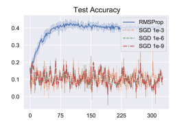
Figure 10: Test set performance of the wide- and narrow Fashion-MNIST ReLU MLP (left and middle) as well as on the CIFAR-10 stripped ResNet500 (right). It becomes evident that RMSProp heavily overfits in the stripped ResNet, which is not surprising given that the network has no regularization what so ever and memorizing CIFAR-10 is comparatively easy for such large convnets.
Refer to caption
Refer to caption
Figure 11: Addendum to Fig. 6. Hessians of fully convolutional ReLU networks of depth L=128𝐿128L=128 on downscaled CIFAR-10 samples at random initializatio (He init.). Contrary to the MLP case in Fig. 4, the Hessians are no longer approximately block-hollow but approximately hollow. Furthermore, as expected, the hollowness decreases in network width (left to right).
Refer to caption
Refer to caption
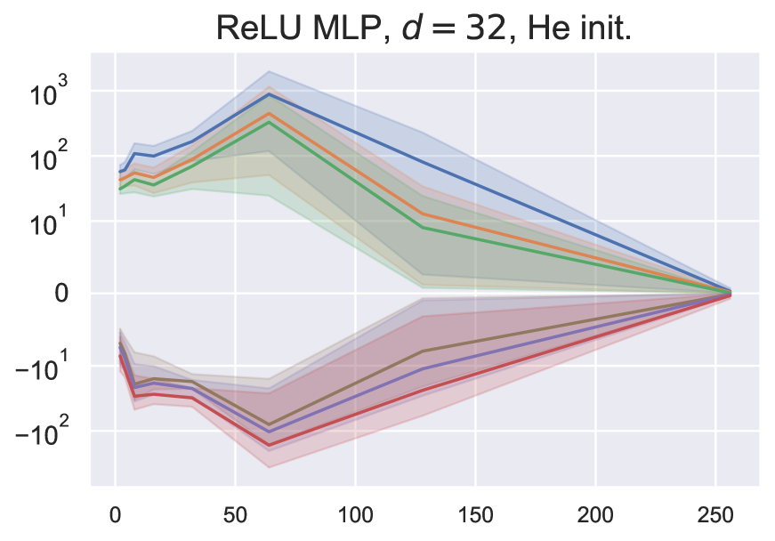
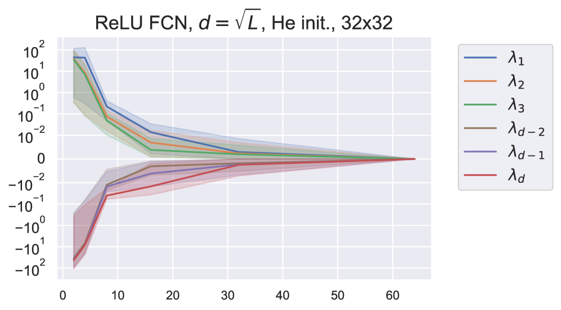
Figure 12: Eigenvalues over depth: Largest (λ1,λ2,λ3subscript𝜆1subscript𝜆2subscript𝜆3\lambda_{1},\lambda_{2},\lambda_{3}) and smallest (λd2,λd1,λdsubscript𝜆𝑑2subscript𝜆𝑑1subscript𝜆𝑑\lambda_{d-2},\lambda_{d-1},\lambda_{d}) three eigenvalues on a symlog scale over depth. Left: ReLU MLPs of width 32. Right: ReLU FCNs of d=L𝑑𝐿d=\sqrt{L}. Both on Fashion-MNIST. Mean and 95%percent\% CI of 5 random seeds.
Refer to caption
Figure 13: Addendum to Fig. 4. Vanishing gradient and Hessian for deep ReLU MLPs with LeCun init.. x-axis depicts depth and width of the networks. Mean and 95%percent\% CI of 10 random seeds.
Refer to caption
Refer to caption
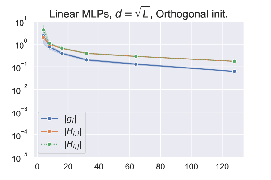
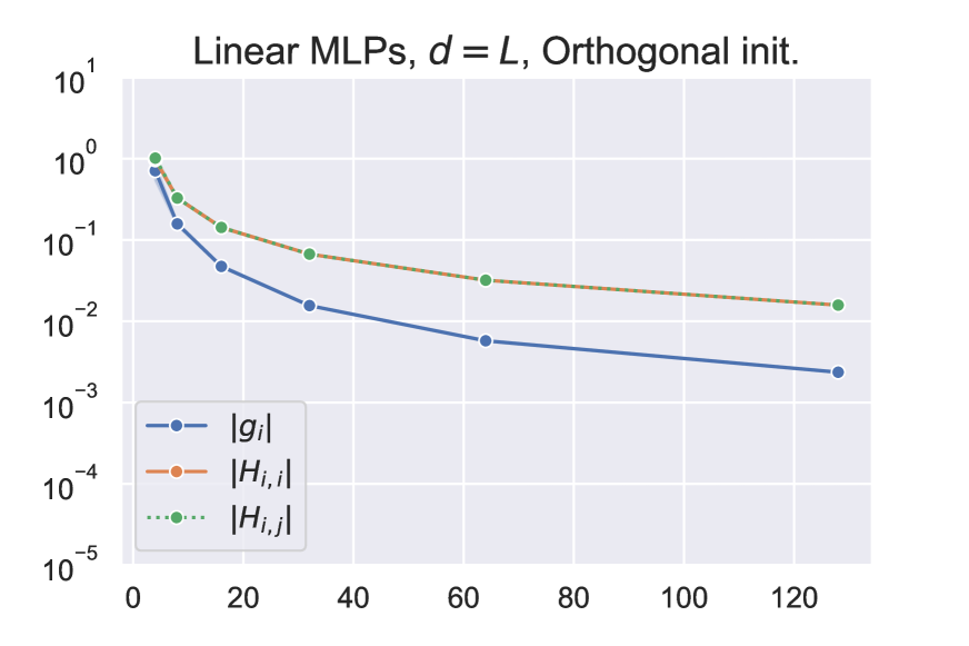
Figure 14: Addendum to Fig. 1: Gradient/curvature on linear MLPs over depth initialized with orthogonal initialization (Saxe et al., 2013). This strategy is very robust towards gradient/curvature vanishing on linear MLPs but quickly yields absolute zeros on ReLU MLPs (PyTorch implementation (Paszke et al., 2019), not shown). Mean and 95% CI of 15 runs.
Refer to caption

depth

Refer to caption

depth

Figure 15: Addendum to Fig. 1: Effect of width in linear MLPs: Gradient and curvature scaling on Fashion-MNIST over depth. While quantities vanish on the left, where the width scales only as square-root of depth, the right shows stable behaviour. Mean and 95% CI of 15 runs.
Refer to caption
Refer to caption
Figure 16: Addendum to Figure 6: Gradient/curvature on FCNs over depth at large resolution (32x32). Mean and 95% CI of 15 runs.
Refer to caption
Refer to caption
Refer to caption
Figure 17: Addendum to Fig. 1: Gradient and Hessian magnitudes in ReLU MLPs over depth. Depicted is the ReLU MLP with d=L𝑑𝐿d=\sqrt{L} and He init. Here, we add Batch Normalization and skip connections to the network.
Refer to caption
Refer to caption
Refer to caption
Figure 18: Addendum to Fig. 6: Gradient and Hessian magnitudes in FCNs over depth. Depicted is the ReLU FCN with d=L𝑑𝐿d=\sqrt{L} at 7×7777\times 7 resolution initialized with He init. (Compare 6 top right). Here, we add Batch Normalization and skip connections to the network.
Refer to caption
Refer to caption
Refer to caption
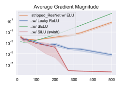
Figure 19: Addendum to Fig. 7: Left: Including original ResNet architecture (i.e. with BN and skip connections). Middle: original ResNet plus version with just BN or Skip connections.Right: Effect of different activations functions in stripped ResNets.
Refer to caption
Refer to caption
Refer to caption
Figure 20: Behavior of the variable 𝐖L𝐖L1𝐖1𝟏22subscriptsuperscriptnormsuperscript𝐖𝐿superscript𝐖𝐿1superscript𝐖1122\|{\bf W}^{L}{\bf W}^{L-1}\cdots{\bf W}^{1}\mathbf{1}\|^{2}_{2}. Entries randomly sampled 𝒰([τ,τ])𝒰𝜏𝜏\mathcal{U}([-\tau,\tau]). Only 505050 samples are shown, but 106superscript10610^{6} are used to approximate population quantities. The expectation is by rare events, and is drastically different from the median if dLmuch-less-than𝑑𝐿d\ll L, as shown in Thm. 9.
Refer to caption
Refer to caption
Refer to caption
Refer to caption
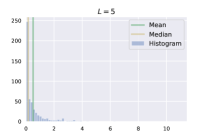
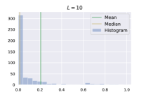
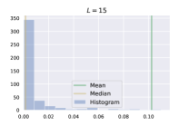
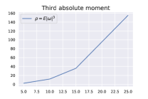
Figure 21: Empirical distribution of products of an increasing number (L𝐿L) of random uniforms. As can be seen the distribution becomes more fat-tailed as L𝐿L increases and the mean and median grow further apart (x𝑥x-axis is capped at 75 times median in all plots). The last plot shows the increase in the third absolute moment over L𝐿L.

Appendix B Analysis of deep linear and ReLU Networks

Note: the fundamental result of this Section (Thm. 17) is checked numerically in Figure 22.

B.1 Notation and fundamental properties

Notation.

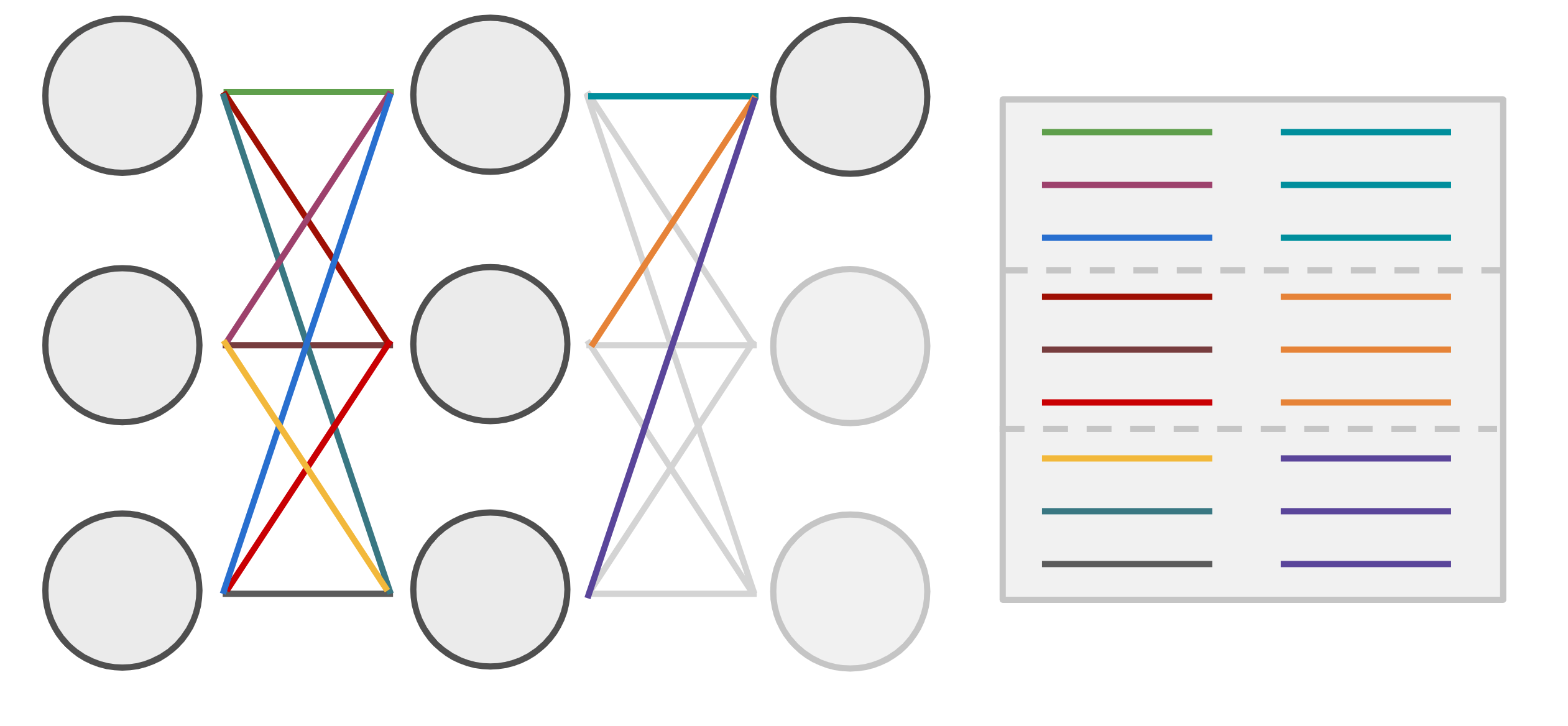
[Uncaptioned image]

In this section, we use neural network notations similar to the one in (Allen-Zhu et al., 2019). In particular,

F(𝐱):=𝐁𝐃L𝐖ϕL:1𝐀𝐱,𝐖ϕL:1:=𝐖L𝐃L1𝐖L1𝐖2𝐃1𝐖1𝐃0,formulae-sequenceassign𝐹𝐱superscript𝐁𝐃𝐿subscriptsuperscript𝐖:𝐿1italic-ϕ𝐀𝐱assignsuperscriptsubscript𝐖italic-ϕ:𝐿1superscript𝐖𝐿superscript𝐃𝐿1superscript𝐖𝐿1superscript𝐖2superscript𝐃1superscript𝐖1superscript𝐃0\displaystyle F({\bf x}):={\bf B}{\bf D}^{L}{\bf W}^{L:1}_{\phi}{\bf A}{\bf x},\quad{\bf W}_{\phi}^{L:1}:={\bf W}^{L}{\bf D}^{L-1}{\bf W}^{L-1}\cdots{\bf W}^{2}{\bf D}^{1}{\bf W}^{1}{\bf D}^{0}, (8)

where F(𝐱)𝐹𝐱F({\bf x}) constitutes the forward pass of a given input 𝐱din𝐱superscriptsubscript𝑑𝑖𝑛{\bf x}\in\mathbb{R}^{d_{in}}, 𝐀d×din𝐀superscript𝑑subscript𝑑𝑖𝑛{\bf A}\in\mathbb{R}^{d\times d_{in}},𝐁dout×d𝐁superscriptsubscript𝑑𝑜𝑢𝑡𝑑{\bf B}\in\mathbb{R}^{d_{out}\times d}, and 𝐖d×d,=1,,Lformulae-sequencesuperscript𝐖superscript𝑑𝑑for-all1𝐿{\bf W}^{\ell}\in{\mathbb{R}}^{d\times d},\forall\ell=1,\ldots,L . 𝐃superscript𝐃{\bf D}^{\ell} is the diagonal matrix of activation gates w.r.t the non-linearity ϕitalic-ϕ\phi at layer \ell, which we consider to be either ϕ(x)=xitalic-ϕ𝑥𝑥\phi(x)=x (linear networks) or ϕ(x)=max{x,0}italic-ϕ𝑥𝑥0\phi(x)=\max\{x,0\} (ReLU networks). Finally, we denote by 𝐚superscript𝐚{\bf a}^{\ell} and 𝐡superscript𝐡{\bf h}^{\ell} the pre- and post activations in layer \ell respectively, i.e. for example 𝐚1=𝐀𝐱superscript𝐚1𝐀𝐱{\bf a}^{1}={\bf A}{\bf x} and 𝐡1=𝐃0𝐚1superscript𝐡1superscript𝐃0superscript𝐚1{\bf h}^{1}={\bf D}^{0}{\bf a}^{1}.

Fundamental properties of activations and preactivations at each layer

Lemma 12 (Fundamental properties of activations and preactivations at each layer).
Let the entries of 𝐀𝐀{\bf A}, 𝐁𝐁{\bf B} and each 𝐖superscript𝐖{\bf W}^{\ell} be i.i.d. samples from a symmetric distribution around 0 with finite moments, and variance σ2superscript𝜎2\sigma^{2}. Then for any fixed input 𝐱𝐱{\bf x}, we have 1. At each layer, entries of the preactivation vector are integrable and have a distribution symmetric around zero. 2. For ReLU networks, at each layer, the entries of the activation vector are non-zero with probability 1/2121/2. 3. At each layer, in both the ReLU and the linear case, the preactivation and the activation vectors have uncorrelated squared entries.
Proof.

Recall that the preactivation at each layer is 𝐚+1=𝐖𝐡superscript𝐚1superscript𝐖superscript𝐡{\bf a}^{\ell+1}={\bf W}^{\ell}{\bf h}^{\ell}. Clearly, since 𝐖=𝐖superscript𝐖superscript𝐖{\bf W}^{\ell}=-{\bf W}^{\ell} in distribution, 𝐚+1=𝐚+1superscript𝐚1superscript𝐚1{\bf a}^{\ell+1}=-{\bf a}^{\ell+1} in distribution. From this follows also that, if a ReLU is applied, 𝐡+1>0superscript𝐡10{\bf h}^{\ell+1}>0 with probability 1/2121/2. The last property to show is that squared entries of activations and preactivations are uncorrelated. Let’s drop the layer index \ell and pick two neurons ij𝑖𝑗i\neq j, then

𝔼[(gi)2(gj)2]=r,s,u,v𝔼[wirwis]𝔼[wjuwjv]𝔼[hrhshuhv]=σ4r,u𝔼[(hr)2(hu)2].𝔼delimited-[]superscriptsubscript𝑔𝑖2superscriptsubscript𝑔𝑗2subscript𝑟𝑠𝑢𝑣𝔼delimited-[]subscript𝑤𝑖𝑟subscript𝑤𝑖𝑠𝔼delimited-[]subscript𝑤𝑗𝑢subscript𝑤𝑗𝑣𝔼delimited-[]subscript𝑟subscript𝑠subscript𝑢subscript𝑣superscript𝜎4subscript𝑟𝑢𝔼delimited-[]superscriptsubscript𝑟2superscriptsubscript𝑢2{\mathbb{E}}[(g_{i})^{2}(g_{j})^{2}]=\sum_{r,s,u,v}{\mathbb{E}}\left[w_{ir}w_{is}\right]{\mathbb{E}}\left[w_{ju}w_{jv}\right]{\mathbb{E}}\left[h_{r}h_{s}h_{u}h_{v}\right]=\sigma^{4}\sum_{r,u}{\mathbb{E}}\left[(h_{r})^{2}(h_{u})^{2}\right]. (9)

Instead, for the single squared variables we have

𝔼[(gi)2]=r,s𝔼[wirwis]𝔼[hrhs]=σ2r𝔼[(hr)2].𝔼delimited-[]superscriptsubscript𝑔𝑖2subscript𝑟𝑠𝔼delimited-[]subscript𝑤𝑖𝑟subscript𝑤𝑖𝑠𝔼delimited-[]subscript𝑟subscript𝑠superscript𝜎2subscript𝑟𝔼delimited-[]superscriptsubscript𝑟2{\mathbb{E}}[(g_{i})^{2}]=\sum_{r,s}{\mathbb{E}}\left[w_{ir}w_{is}\right]{\mathbb{E}}\left[h_{r}h_{s}\right]=\sigma^{2}\sum_{r}{\mathbb{E}}\left[(h_{r})^{2}\right]. (10)

Therefore 𝔼[(gi)2(gj)2]=𝔼[(gi)2]𝔼[(gj)2]𝔼delimited-[]superscriptsubscript𝑔𝑖2superscriptsubscript𝑔𝑗2𝔼delimited-[]superscriptsubscript𝑔𝑖2𝔼delimited-[]superscriptsubscript𝑔𝑗2{\mathbb{E}}[(g_{i})^{2}(g_{j})^{2}]={\mathbb{E}}[(g_{i})^{2}]{\mathbb{E}}[(g_{j})^{2}] if and only if (hi)2superscriptsubscript𝑖2(h_{i})^{2} and (hj)2superscriptsubscript𝑗2(h_{j})^{2} are uncorrelated. As 𝐱𝐱{\bf x} is fixed, this is the case at the input layer and we conclude the proof by induction on \ell.

Last, we show the same properties for the activations in the ReLU case. Let di=ϕ(gi)/gi=𝟙(gi>0)subscript𝑑𝑖italic-ϕsubscript𝑔𝑖subscript𝑔𝑖1subscript𝑔𝑖0d_{i}=\phi(g_{i})/g_{i}=\mathbbm{1}{(g_{i}>0)} and consider the new activation hi+=digisubscriptsuperscript𝑖subscript𝑑𝑖subscript𝑔𝑖h^{+}_{i}=d_{i}g_{i}. We start by applying the law of total expectation:

𝔼[(hi+)2(hj+)2]=𝔼[(di)2(dj)2(gi)2(gj)2]=14𝔼[(gi)2(gj)2|di,dj=1]\displaystyle{\mathbb{E}}[(h_{i}^{+})^{2}(h_{j}^{+})^{2}]={\mathbb{E}}\left[(d_{i})^{2}(d_{j})^{2}(g_{i})^{2}(g_{j})^{2}\right]=\frac{1}{4}{\mathbb{E}}\left[(g_{i})^{2}(g_{j})^{2}\lvert d_{i},d_{j}=1\right] (11)
=14𝔼[(gi)2(gj)2]=12𝔼[(gi)2]12𝔼[(gj)2]=𝔼[(hi+)2]𝔼[(hj+)2],absent14𝔼delimited-[]superscriptsubscript𝑔𝑖2superscriptsubscript𝑔𝑗212𝔼delimited-[]superscriptsubscript𝑔𝑖212𝔼delimited-[]superscriptsubscript𝑔𝑗2𝔼delimited-[]superscriptsuperscriptsubscript𝑖2𝔼delimited-[]superscriptsuperscriptsubscript𝑗2\displaystyle=\frac{1}{4}{\mathbb{E}}\left[(g_{i})^{2}(g_{j})^{2}\right]=\frac{1}{2}{\mathbb{E}}\left[(g_{i})^{2}\right]\frac{1}{2}{\mathbb{E}}\left[(g_{j})^{2}\right]={\mathbb{E}}[(h_{i}^{+})^{2}]{\mathbb{E}}[(h_{j}^{+})^{2}],

where the third and the last equalities follow from the fact that the value of the squared preactivation is independent on the sign of the preactivation. ∎

Statistics for the propagation through one layer

Lemma 13 (Statistics after activation function).
Let 𝐱𝐱{\bf x} be a symmetric random vector with uncorrelated squared entries. Let ϕ(𝐱)=𝐃𝐱𝐱italic-ϕ𝐱subscript𝐃𝐱𝐱\phi({\bf x})={\bf D}_{{\bf x}}{\bf x}. We have 𝔼𝐃𝐱𝐱22𝔼superscriptsubscriptnormsubscript𝐃𝐱𝐱22\displaystyle{\mathbb{E}}\|{\bf D}_{{\bf x}}{\bf x}\|_{2}^{2} =p𝔼𝐱22;absent𝑝𝔼superscriptsubscriptnorm𝐱22\displaystyle=p\ {\mathbb{E}}\|{\bf x}\|_{2}^{2}; (12) 𝔼𝐃𝐱𝐱24𝔼superscriptsubscriptnormsubscript𝐃𝐱𝐱24\displaystyle{\mathbb{E}}\|{\bf D}_{{\bf x}}{\bf x}\|_{2}^{4} =p2𝔼𝐱24+(pp2)𝔼𝐱44;absentsuperscript𝑝2𝔼superscriptsubscriptnorm𝐱24𝑝superscript𝑝2𝔼superscriptsubscriptnorm𝐱44\displaystyle=p^{2}{\mathbb{E}}\|{\bf x}\|_{2}^{4}+(p-p^{2}){\mathbb{E}}\|{\bf x}\|_{4}^{4}; (13) 𝔼𝐃𝐱𝐱44𝔼superscriptsubscriptnormsubscript𝐃𝐱𝐱44\displaystyle{\mathbb{E}}\|{\bf D}_{{\bf x}}{\bf x}\|_{4}^{4} =p𝔼𝐱44.absent𝑝𝔼superscriptsubscriptnorm𝐱44\displaystyle=p\ {\mathbb{E}}\|{\bf x}\|_{4}^{4}. (14) where p=1𝑝1p=1 for linear nets and p=1/2𝑝12p=1/2 for ReLU nets.
Proof.

The first property is based on the fundamental idea in (He et al., 2015). Let disubscript𝑑𝑖d_{i} be the entry (i,i)𝑖𝑖(i,i) of 𝐃𝐱subscript𝐃𝐱{\bf D}_{{\bf x}}. Then, disubscript𝑑𝑖d_{i} is independent from xi2superscriptsubscript𝑥𝑖2x_{i}^{2}. Hence, also noting that (di)2=disuperscriptsubscript𝑑𝑖2subscript𝑑𝑖(d_{i})^{2}=d_{i}, we have

𝔼𝐃𝐱𝐱22=i𝔼[di2xi2]=i𝔼[di]𝔼[xi2]=p𝔼𝐱22.𝔼superscriptsubscriptnormsubscript𝐃𝐱𝐱22subscript𝑖𝔼delimited-[]superscriptsubscript𝑑𝑖2superscriptsubscript𝑥𝑖2subscript𝑖𝔼delimited-[]subscript𝑑𝑖𝔼delimited-[]superscriptsubscript𝑥𝑖2𝑝𝔼superscriptsubscriptnorm𝐱22{\mathbb{E}}\|{\bf D}_{{\bf x}}{\bf x}\|_{2}^{2}=\sum_{i}{\mathbb{E}}\left[d_{i}^{2}x_{i}^{2}\right]=\sum_{i}{\mathbb{E}}\left[d_{i}\right]{\mathbb{E}}\left[x_{i}^{2}\right]=p\ {\mathbb{E}}\|{\bf x}\|_{2}^{2}. (15)

where p=𝔼[di]𝑝𝔼delimited-[]subscript𝑑𝑖p={\mathbb{E}}[d_{i}], which is 1/2121/2 for ReLU nets and 111 for linear nets, as shown in Lemma 12. The last property can be proved in the same way by noting that disubscript𝑑𝑖d_{i} is independent from xi4superscriptsubscript𝑥𝑖4x_{i}^{4}

𝔼𝐃𝐱𝐱44=i𝔼[di4xi4]=i𝔼[di]𝔼[xi4]=p𝔼𝐱44.𝔼superscriptsubscriptnormsubscript𝐃𝐱𝐱44subscript𝑖𝔼delimited-[]superscriptsubscript𝑑𝑖4superscriptsubscript𝑥𝑖4subscript𝑖𝔼delimited-[]subscript𝑑𝑖𝔼delimited-[]superscriptsubscript𝑥𝑖4𝑝𝔼superscriptsubscriptnorm𝐱44{\mathbb{E}}\|{\bf D}_{{\bf x}}{\bf x}\|_{4}^{4}=\sum_{i}{\mathbb{E}}\left[d_{i}^{4}x_{i}^{4}\right]=\sum_{i}{\mathbb{E}}\left[d_{i}\right]{\mathbb{E}}\left[x_{i}^{4}\right]=p\ {\mathbb{E}}\|{\bf x}\|_{4}^{4}. (16)

The second property is a bit more involved to prove.

𝔼𝐃𝐱𝐱24=𝔼(i=1d(dixi)2)2=i=1d𝔼[(dixi)4]+ij𝔼[(dixi)2(djxj)2].𝔼superscriptsubscriptnormsubscript𝐃𝐱𝐱24𝔼superscriptsuperscriptsubscript𝑖1𝑑superscriptsubscript𝑑𝑖subscript𝑥𝑖22superscriptsubscript𝑖1𝑑𝔼delimited-[]superscriptsubscript𝑑𝑖subscript𝑥𝑖4subscript𝑖𝑗𝔼delimited-[]superscriptsubscript𝑑𝑖subscript𝑥𝑖2superscriptsubscript𝑑𝑗subscript𝑥𝑗2{\mathbb{E}}\|{\bf D}_{{\bf x}}{\bf x}\|_{2}^{4}={\mathbb{E}}\left(\sum_{i=1}^{d}(d_{i}x_{i})^{2}\right)^{2}=\sum_{i=1}^{d}{\mathbb{E}}\left[(d_{i}x_{i})^{4}\right]+\sum_{i\neq j}{\mathbb{E}}\left[(d_{i}x_{i})^{2}(d_{j}x_{j})^{2}\right]. (17)

From Lemma 12, third point, we have 𝔼[(dixi)2(djxj)2]=𝔼[(dixi)2]𝔼[(djxj)2]𝔼delimited-[]superscriptsubscript𝑑𝑖subscript𝑥𝑖2superscriptsubscript𝑑𝑗subscript𝑥𝑗2𝔼delimited-[]superscriptsubscript𝑑𝑖subscript𝑥𝑖2𝔼delimited-[]superscriptsubscript𝑑𝑗subscript𝑥𝑗2{\mathbb{E}}\left[(d_{i}x_{i})^{2}(d_{j}x_{j})^{2}\right]={\mathbb{E}}\left[(d_{i}x_{i})^{2}\right]{\mathbb{E}}\left[(d_{j}x_{j})^{2}\right] (compare Eq.(11)). Hence, noting again that di=di2subscript𝑑𝑖superscriptsubscript𝑑𝑖2d_{i}=d_{i}^{2},

𝔼𝐃𝐱𝐱24𝔼superscriptsubscriptnormsubscript𝐃𝐱𝐱24\displaystyle{\mathbb{E}}\|{\bf D}_{{\bf x}}{\bf x}\|_{2}^{4} =i=1d𝔼[di]𝔼[xi4]+ij𝔼[di]𝔼[dj]𝔼[xi2xj2]absentsuperscriptsubscript𝑖1𝑑𝔼delimited-[]subscript𝑑𝑖𝔼delimited-[]superscriptsubscript𝑥𝑖4subscript𝑖𝑗𝔼delimited-[]subscript𝑑𝑖𝔼delimited-[]subscript𝑑𝑗𝔼delimited-[]superscriptsubscript𝑥𝑖2superscriptsubscript𝑥𝑗2\displaystyle=\sum_{i=1}^{d}{\mathbb{E}}\left[d_{i}\right]{\mathbb{E}}\left[x_{i}^{4}\right]+\sum_{i\neq j}{\mathbb{E}}\left[d_{i}\right]{\mathbb{E}}\left[d_{j}\right]{\mathbb{E}}\left[x_{i}^{2}x_{j}^{2}\right] (18)
=p𝔼𝐱44+p2𝔼[𝐱24𝐱44].absent𝑝𝔼subscriptsuperscriptnorm𝐱44superscript𝑝2𝔼delimited-[]subscriptsuperscriptnorm𝐱42subscriptsuperscriptnorm𝐱44\displaystyle=p\ {\mathbb{E}}\|{\bf x}\|^{4}_{4}+p^{2}{\mathbb{E}}\left[\|{\bf x}\|^{4}_{2}-\|{\bf x}\|^{4}_{4}\right]. (19)

This concludes the proof. ∎

The following corollary is of fundamental importance of understanding the properties of ReLU nets: if the input of the net is modified, the ReLU gates act as purely random Bernoulli gates. This comment can be also found in the proof of Lemma A.8 in (Zou et al., 2020).

Corollary 14 (Statistics after activation function with changed input).
In the context of Lemma 13, let 𝛂𝛂{\boldsymbol{\alpha}} be a fixed vector. we have 𝔼𝐃𝐱𝜶22𝔼superscriptsubscriptnormsubscript𝐃𝐱𝜶22\displaystyle{\mathbb{E}}\|{\bf D}_{{\bf x}}{\boldsymbol{\alpha}}\|_{2}^{2} =p𝜶22;absent𝑝superscriptsubscriptnorm𝜶22\displaystyle=p\ \|{\boldsymbol{\alpha}}\|_{2}^{2}; (20) 𝔼𝐃𝐱𝜶24𝔼superscriptsubscriptnormsubscript𝐃𝐱𝜶24\displaystyle{\mathbb{E}}\|{\bf D}_{{\bf x}}{\boldsymbol{\alpha}}\|_{2}^{4} =p2𝜶24+(pp2)𝜶44;absentsuperscript𝑝2superscriptsubscriptnorm𝜶24𝑝superscript𝑝2superscriptsubscriptnorm𝜶44\displaystyle=p^{2}\|{\boldsymbol{\alpha}}\|_{2}^{4}+(p-p^{2})\|{\boldsymbol{\alpha}}\|_{4}^{4}; (21) 𝔼𝐃𝐱𝜶44𝔼superscriptsubscriptnormsubscript𝐃𝐱𝜶44\displaystyle{\mathbb{E}}\|{\bf D}_{{\bf x}}{\boldsymbol{\alpha}}\|_{4}^{4} =p𝜶44.absent𝑝superscriptsubscriptnorm𝜶44\displaystyle=p\ \|{\boldsymbol{\alpha}}\|_{4}^{4}. (22) where p=1𝑝1p=1 for linear nets and p=1/2𝑝12p=1/2 for ReLU nets.
Proof.

Just note that since 𝐃𝐱subscript𝐃𝐱{\bf D}_{{\bf x}} and 𝜶𝜶{\boldsymbol{\alpha}} are independent we can basically follow the proof of Lemma 13, but simplified:

𝔼𝐃𝐱𝜶mm=i𝔼[dimαim]=i𝔼[di]αim=p𝜶mm.𝔼superscriptsubscriptnormsubscript𝐃𝐱𝜶𝑚𝑚subscript𝑖𝔼delimited-[]superscriptsubscript𝑑𝑖𝑚superscriptsubscript𝛼𝑖𝑚subscript𝑖𝔼delimited-[]subscript𝑑𝑖superscriptsubscript𝛼𝑖𝑚𝑝superscriptsubscriptnorm𝜶𝑚𝑚{\mathbb{E}}\|{\bf D}_{{\bf x}}{\boldsymbol{\alpha}}\|_{m}^{m}=\sum_{i}{\mathbb{E}}\left[d_{i}^{m}\alpha_{i}^{m}\right]=\sum_{i}{\mathbb{E}}\left[d_{i}\right]\alpha_{i}^{m}=p\ \|{\boldsymbol{\alpha}}\|_{m}^{m}. (23)

The second property is also easy to show compared to Lemma 13:

𝔼𝐃𝐱𝜶24𝔼superscriptsubscriptnormsubscript𝐃𝐱𝜶24\displaystyle{\mathbb{E}}\|{\bf D}_{{\bf x}}{\boldsymbol{\alpha}}\|_{2}^{4} =𝔼(i=1d(diαi)2)2absent𝔼superscriptsuperscriptsubscript𝑖1𝑑superscriptsubscript𝑑𝑖subscript𝛼𝑖22\displaystyle={\mathbb{E}}\left(\sum_{i=1}^{d}(d_{i}\alpha_{i})^{2}\right)^{2} (24)
=i=1d𝔼[(diαi)4]+ij𝔼[(diαi)2(djαj)2]absentsuperscriptsubscript𝑖1𝑑𝔼delimited-[]superscriptsubscript𝑑𝑖subscript𝛼𝑖4subscript𝑖𝑗𝔼delimited-[]superscriptsubscript𝑑𝑖subscript𝛼𝑖2superscriptsubscript𝑑𝑗subscript𝛼𝑗2\displaystyle=\sum_{i=1}^{d}{\mathbb{E}}\left[(d_{i}\alpha_{i})^{4}\right]+\sum_{i\neq j}{\mathbb{E}}\left[(d_{i}\alpha_{i})^{2}(d_{j}\alpha_{j})^{2}\right] (25)
=i=1d𝔼[di]αi4+ij𝔼[di]𝔼[dj]αi2αj2.absentsuperscriptsubscript𝑖1𝑑𝔼delimited-[]subscript𝑑𝑖superscriptsubscript𝛼𝑖4subscript𝑖𝑗𝔼delimited-[]subscript𝑑𝑖𝔼delimited-[]subscript𝑑𝑗superscriptsubscript𝛼𝑖2superscriptsubscript𝛼𝑗2\displaystyle=\sum_{i=1}^{d}{\mathbb{E}}\left[d_{i}\right]\alpha_{i}^{4}+\sum_{i\neq j}{\mathbb{E}}[d_{i}]{\mathbb{E}}[d_{j}]\alpha_{i}^{2}\alpha_{j}^{2}. (26)

This concludes the proof. ∎

Next, we study the change in statistics after multiplication with a random matrix.

Lemma 15 (Statistics after multiplication with a random matrix).
Let 𝐖𝐖{\bf W} be an iid random matrix, with zero mean entries that have variance σ2superscript𝜎2\sigma^{2} and kurtosis κ𝜅\kappa. Let 𝛏d𝛏superscript𝑑{\boldsymbol{\xi}}\in{\mathbb{R}}^{d} be an arbitrary random vector (not necessarily symmetric or with uncorrelated squared entries). Then 𝔼𝐖𝝃22=dσ2𝔼𝝃2;𝔼superscriptsubscriptnorm𝐖𝝃22𝑑superscript𝜎2𝔼superscriptnorm𝝃2\displaystyle{\mathbb{E}}\|{\bf W}{\boldsymbol{\xi}}\|_{2}^{2}=d\sigma^{2}{\mathbb{E}}\|{\boldsymbol{\xi}}\|^{2}; (27) 𝔼𝐖𝝃24=d(d+2)σ4𝔼𝝃24+(κ3)dσ4𝔼𝝃44;𝔼superscriptsubscriptnorm𝐖𝝃24𝑑𝑑2superscript𝜎4𝔼superscriptsubscriptnorm𝝃24𝜅3𝑑superscript𝜎4𝔼subscriptsuperscriptnorm𝝃44\displaystyle{\mathbb{E}}\|{\bf W}\mathbf{{\boldsymbol{\xi}}}\|_{2}^{4}=d(d+2)\sigma^{4}{\mathbb{E}}\|{\boldsymbol{\xi}}\|_{2}^{4}+(\kappa-3)d\sigma^{4}{\mathbb{E}}\|{\boldsymbol{\xi}}\|^{4}_{4}; (28) 𝔼𝐖𝝃44=3dσ4𝔼𝝃24+(κ3)dσ4𝔼𝝃44.𝔼superscriptsubscriptnorm𝐖𝝃443𝑑superscript𝜎4𝔼superscriptsubscriptnorm𝝃24𝜅3𝑑superscript𝜎4𝔼superscriptsubscriptnorm𝝃44\displaystyle{\mathbb{E}}\|{\bf W}{\boldsymbol{\xi}}\|_{4}^{4}=3d\sigma^{4}{\mathbb{E}}\|{\boldsymbol{\xi}}\|_{2}^{4}+(\kappa-3)d\sigma^{4}{\mathbb{E}}\|{\boldsymbol{\xi}}\|_{4}^{4}. (29)
Proof.

The first property is easy to show:

𝔼𝐖𝝃22=𝔼r(s,uwrsξswruξu)=𝔼r(swrs2ξs2)=dσ2𝔼𝝃2.𝔼superscriptsubscriptnorm𝐖𝝃22𝔼subscript𝑟subscript𝑠𝑢subscript𝑤𝑟𝑠subscript𝜉𝑠subscript𝑤𝑟𝑢subscript𝜉𝑢𝔼subscript𝑟subscript𝑠superscriptsubscript𝑤𝑟𝑠2superscriptsubscript𝜉𝑠2𝑑superscript𝜎2𝔼superscriptnorm𝝃2{\mathbb{E}}\|{\bf W}{\boldsymbol{\xi}}\|_{2}^{2}={\mathbb{E}}\sum_{r}\left(\sum_{s,u}w_{rs}\xi_{s}w_{ru}\xi_{u}\right)={\mathbb{E}}\sum_{r}\left(\sum_{s}w_{rs}^{2}\xi_{s}^{2}\right)=d\sigma^{2}{\mathbb{E}}\|{\boldsymbol{\xi}}\|^{2}. (30)

The second and the third properties need computations.

𝐖𝝃24superscriptsubscriptnorm𝐖𝝃24\displaystyle\|{\bf W}{\boldsymbol{\xi}}\|_{2}^{4} =(i(rwirξr)2)2absentsuperscriptsubscript𝑖superscriptsubscript𝑟subscript𝑤𝑖𝑟subscript𝜉𝑟22\displaystyle=\Big{(}\sum_{i}\Big{(}\sum_{r}w_{ir}\xi_{r}\Big{)}^{2}\Big{)}^{2} (31)
=i,jrwirξrswisξsuwjuξuvwjvξv,absentsubscript𝑖𝑗subscript𝑟subscript𝑤𝑖𝑟subscript𝜉𝑟subscript𝑠subscript𝑤𝑖𝑠subscript𝜉𝑠subscript𝑢subscript𝑤𝑗𝑢subscript𝜉𝑢subscript𝑣subscript𝑤𝑗𝑣subscript𝜉𝑣\displaystyle=\sum_{i,j}\sum_{r}w_{ir}\xi_{r}\sum_{s}w_{is}\xi_{s}\sum_{u}w_{ju}\xi_{u}\sum_{v}w_{jv}\xi_{v}, (32)
𝐖𝝃44subscriptsuperscriptnorm𝐖𝝃44\displaystyle\|{\bf W}{\boldsymbol{\xi}}\|^{4}_{4} =i(rwirξr)4absentsubscript𝑖superscriptsubscript𝑟subscript𝑤𝑖𝑟subscript𝜉𝑟4\displaystyle=\sum_{i}\Big{(}\sum_{r}w_{ir}\xi_{r}\Big{)}^{4} (33)
=irwirξrswisξsuwiuξuvwivξv.absentsubscript𝑖subscript𝑟subscript𝑤𝑖𝑟subscript𝜉𝑟subscript𝑠subscript𝑤𝑖𝑠subscript𝜉𝑠subscript𝑢subscript𝑤𝑖𝑢subscript𝜉𝑢subscript𝑣subscript𝑤𝑖𝑣subscript𝜉𝑣\displaystyle=\sum_{i}\sum_{r}w_{ir}\xi_{r}\sum_{s}w_{is}\xi_{s}\sum_{u}w_{iu}\xi_{u}\sum_{v}w_{iv}\xi_{v}. (34)

Taking expectations, yields

𝔼𝐖𝝃44σ4𝔼superscriptsubscriptnorm𝐖𝝃44superscript𝜎4\displaystyle\frac{{\mathbb{E}}\|{\bf W}{\boldsymbol{\xi}}\|_{4}^{4}}{\sigma^{4}} =κiκd𝔼𝝃44+3i3drs𝔼[ξr2ξs2]𝔼𝝃24𝔼𝝃44=3d𝔼𝝃24+(κ3)d𝔼𝝃44;absentsubscript𝜅subscript𝑖𝜅𝑑𝔼subscriptsuperscriptnorm𝝃44subscript3subscript𝑖3𝑑subscriptsubscript𝑟𝑠𝔼delimited-[]superscriptsubscript𝜉𝑟2superscriptsubscript𝜉𝑠2𝔼subscriptsuperscriptnorm𝝃42𝔼superscriptsubscriptnorm𝝃443𝑑𝔼superscriptsubscriptnorm𝝃24𝜅3𝑑𝔼superscriptsubscriptnorm𝝃44\displaystyle=\underbrace{\kappa\sum_{i}}_{\kappa d}{\mathbb{E}}\|\mathbf{{\boldsymbol{\xi}}}\|^{4}_{4}+\underbrace{3\sum_{i}}_{3d}\underbrace{\sum_{r\neq s}{\mathbb{E}}\left[\xi_{r}^{2}\xi_{s}^{2}\right]}_{{\mathbb{E}}\|{\boldsymbol{\xi}}\|^{4}_{2}-{\mathbb{E}}\|{\boldsymbol{\xi}}\|_{4}^{4}}=3d\ {\mathbb{E}}\|{\boldsymbol{\xi}}\|_{2}^{4}+(\kappa-3)d\ {\mathbb{E}}\|{\boldsymbol{\xi}}\|_{4}^{4}; (35)
𝔼𝐖𝝃24σ4𝔼subscriptsuperscriptnorm𝐖𝝃42superscript𝜎4\displaystyle\frac{{\mathbb{E}}\|{\bf W}{\boldsymbol{\xi}}\|^{4}_{2}}{\sigma^{4}} =ijd(d1)𝔼[(r=sξr2)(u=vξu2)]𝔼𝝃24+3i=j3drs𝔼[ξr2ξs2]𝔼𝝃24𝔼𝝃44+κiκdr=s𝔼[ξr4]𝔼𝝃44absentsubscriptsubscript𝑖𝑗𝑑𝑑1subscript𝔼delimited-[]subscript𝑟𝑠superscriptsubscript𝜉𝑟2subscript𝑢𝑣superscriptsubscript𝜉𝑢2𝔼superscriptsubscriptnorm𝝃24subscript3subscript𝑖𝑗3𝑑subscriptsubscript𝑟𝑠𝔼delimited-[]superscriptsubscript𝜉𝑟2superscriptsubscript𝜉𝑠2𝔼subscriptsuperscriptnorm𝝃42𝔼superscriptsubscriptnorm𝝃44subscript𝜅subscript𝑖𝜅𝑑subscriptsubscript𝑟𝑠𝔼delimited-[]superscriptsubscript𝜉𝑟4𝔼superscriptsubscriptnorm𝝃44\displaystyle=\underbrace{\sum_{i\neq j}}_{d(d-1)}\underbrace{{\mathbb{E}}\left[\Big{(}\sum_{r=s}\xi_{r}^{2}\Big{)}\Big{(}\sum_{u=v}\xi_{u}^{2}\Big{)}\right]}_{{\mathbb{E}}\|{\boldsymbol{\xi}}\|_{2}^{4}}+\underbrace{3\sum_{i=j}}_{3d}\underbrace{\sum_{r\neq s}{\mathbb{E}}\left[\xi_{r}^{2}\xi_{s}^{2}\right]}_{{\mathbb{E}}\|{\boldsymbol{\xi}}\|^{4}_{2}-{\mathbb{E}}\|{\boldsymbol{\xi}}\|_{4}^{4}}+\underbrace{\kappa\sum_{i}}_{\kappa d}\underbrace{\sum_{r=s}{\mathbb{E}}[\xi_{r}^{4}]}_{{\mathbb{E}}\|{\boldsymbol{\xi}}\|_{4}^{4}} (36)
=d(d+2)𝔼𝝃24+(κ3)d𝔼𝝃44.absent𝑑𝑑2𝔼superscriptsubscriptnorm𝝃24𝜅3𝑑𝔼subscriptsuperscriptnorm𝝃44\displaystyle=d(d+2){\mathbb{E}}\|{\boldsymbol{\xi}}\|_{2}^{4}+(\kappa-3)d\ {\mathbb{E}}\|{\boldsymbol{\xi}}\|^{4}_{4}.

The factor 3 appears because, if 444 indices are paired in groups of two, we have a total of 333 disjoint choices: {i=j,u=v}formulae-sequence𝑖𝑗𝑢𝑣\{i=j,u=v\}, {i=u,j=v}formulae-sequence𝑖𝑢𝑗𝑣\{i=u,j=v\}, {i=v,j=u}formulae-sequence𝑖𝑣𝑗𝑢\{i=v,j=u\}. ∎

Corollary 16 (Preactivations after one (ReLU) layer).
Let 𝐱𝐱{\bf x} be a symmetric random vector with uncorrelated squared entries and 𝐖𝐖{\bf W} be an iid random matrix, entries having mean zero, variance σ2superscript𝜎2\sigma^{2} and kurtosis κ𝜅\kappa. Then, the following formulas hold: 𝔼𝐖𝐃𝐱𝐱22=dσ2p𝔼𝐱22;𝔼superscriptsubscriptnormsubscript𝐖𝐃𝐱𝐱22𝑑superscript𝜎2𝑝𝔼superscriptsubscriptnorm𝐱22\displaystyle{\mathbb{E}}\|{\bf W}{\bf D}_{{\bf x}}{\bf x}\|_{2}^{2}=d\sigma^{2}p{\mathbb{E}}\|{\bf x}\|_{2}^{2}; (37) 𝔼𝐖𝐃𝐱𝐱24=[d(d+2)σ4p2]𝔼𝐱24+[dσ4p(κ3+(1p)(d+2))]𝔼𝐱44;𝔼superscriptsubscriptnormsubscript𝐖𝐃𝐱𝐱24delimited-[]𝑑𝑑2superscript𝜎4superscript𝑝2𝔼superscriptsubscriptnorm𝐱24delimited-[]𝑑superscript𝜎4𝑝𝜅31𝑝𝑑2𝔼subscriptsuperscriptnorm𝐱44\displaystyle{\mathbb{E}}\|{\bf W}{\bf D}_{{\bf x}}{\bf x}\|_{2}^{4}=\left[d(d+2)\sigma^{4}p^{2}\right]{\mathbb{E}}\|{\bf x}\|_{2}^{4}+\left[d\sigma^{4}p\left(\kappa-3+(1-p)(d+2)\right)\right]{\mathbb{E}}\|{\bf x}\|^{4}_{4}; (38) 𝔼𝐖𝐃𝐱𝐱44=[3dσ4p2]𝔼𝐱24+[dσ4p(κ3p)]𝔼𝐱44.𝔼superscriptsubscriptnormsubscript𝐖𝐃𝐱𝐱44delimited-[]3𝑑superscript𝜎4superscript𝑝2𝔼superscriptsubscriptnorm𝐱24delimited-[]𝑑superscript𝜎4𝑝𝜅3𝑝𝔼subscriptsuperscriptnorm𝐱44\displaystyle{\mathbb{E}}\|{\bf W}{\bf D}_{{\bf x}}{\bf x}\|_{4}^{4}=\left[3d\sigma^{4}p^{2}\right]{\mathbb{E}}\|{\bf x}\|_{2}^{4}+\left[d\sigma^{4}p(\kappa-3p)\right]{\mathbb{E}}\|{\bf x}\|^{4}_{4}. (39)
Proof.

Follows directly from Lemma 15 by plugging in 𝝃=𝐃𝐱𝐱𝝃subscript𝐃𝐱𝐱{\boldsymbol{\xi}}={\bf D}_{{\bf x}}{\bf x}. The effect of the potential ReLU is then integrated out using Lemma 13. ∎

B.2 Forward pass

The next theorem, which is the fundamental tool for our analysis, is checked numerically in Figure 22.

Theorem 17 (Forward pass statistics).
Let 𝐳=𝐀𝐱𝐳𝐀𝐱{\bf z}={\bf A}{\bf x}, which is, for 𝐱𝐱{\bf x} fixed, symmetrically distributed and with uncorrelated squared entries. Then, 𝔼𝐖ϕk:1𝐳22𝔼superscriptsubscriptnormsubscriptsuperscript𝐖:𝑘1italic-ϕ𝐳22\displaystyle{\mathbb{E}}\|\mathbf{W}^{k:1}_{\phi}{\bf z}\|_{2}^{2} =(dσ2p)k𝔼𝐳22;absentsuperscript𝑑superscript𝜎2𝑝𝑘𝔼subscriptsuperscriptnorm𝐳22\displaystyle=(d\sigma^{2}p)^{k}{\mathbb{E}}\|{\bf z}\|^{2}_{2}; (40) (𝔼𝐖ϕk:1𝐳24𝔼𝐖ϕk:1𝐳44)matrix𝔼superscriptsubscriptnormsubscriptsuperscript𝐖:𝑘1italic-ϕ𝐳24𝔼superscriptsubscriptnormsubscriptsuperscript𝐖:𝑘1italic-ϕ𝐳44\displaystyle\begin{pmatrix}{\mathbb{E}}\|\mathbf{W}^{k:1}_{\phi}{\bf z}\|_{2}^{4}\\ {\mathbb{E}}\|\mathbf{W}^{k:1}_{\phi}{\bf z}\|_{4}^{4}\end{pmatrix} =(p2dσ4)k𝐐k(𝔼𝐳24𝔼𝐳44),𝐐:=(d+2κ3+(1p)(d+2)p3κ3pp).formulae-sequenceabsentsuperscriptsuperscript𝑝2𝑑superscript𝜎4𝑘superscript𝐐𝑘matrix𝔼superscriptsubscriptnorm𝐳24𝔼superscriptsubscriptnorm𝐳44assign𝐐matrix𝑑2𝜅31𝑝𝑑2𝑝3𝜅3𝑝𝑝\displaystyle=\left(p^{2}d\sigma^{4}\right)^{k}{\bf Q}^{k}\begin{pmatrix}{\mathbb{E}}\|{\bf z}\|_{2}^{4}\\ {\mathbb{E}}\|{\bf z}\|_{4}^{4}\end{pmatrix},\quad{\bf Q}:=\begin{pmatrix}d+2&\frac{\kappa-3+(1-p)(d+2)}{p}\\ 3&\frac{\kappa-3p}{p}\end{pmatrix}. (41)
Proof.

From Lemma 12 we know that at initialization the entries of layer preactivations are symmetrically distributed and with uncorrelated squared entries. Hence, we can apply Corollary  16 recursively to preactivations.

𝔼𝐖ϕk:1𝐳22=dσ2p𝔼𝐖ϕk1:1𝐳22;𝔼superscriptsubscriptnormsubscriptsuperscript𝐖:𝑘1italic-ϕ𝐳22𝑑superscript𝜎2𝑝𝔼superscriptsubscriptnormsubscriptsuperscript𝐖:𝑘11italic-ϕ𝐳22\displaystyle{\mathbb{E}}\|\mathbf{W}^{k:1}_{\phi}{\bf z}\|_{2}^{2}=d\sigma^{2}p{\mathbb{E}}\|\mathbf{W}^{k-1:1}_{\phi}{\bf z}\|_{2}^{2}; (42)
𝔼𝐖ϕk:1𝐳24=[d(d+2)σ4p2]𝔼𝐖ϕk1:1𝐳24𝔼superscriptsubscriptnormsubscriptsuperscript𝐖:𝑘1italic-ϕ𝐳24delimited-[]𝑑𝑑2superscript𝜎4superscript𝑝2𝔼superscriptsubscriptnormsubscriptsuperscript𝐖:𝑘11italic-ϕ𝐳24\displaystyle{\mathbb{E}}\|\mathbf{W}^{k:1}_{\phi}{\bf z}\|_{2}^{4}=\left[d(d+2)\sigma^{4}p^{2}\right]{\mathbb{E}}\|\mathbf{W}^{k-1:1}_{\phi}{\bf z}\|_{2}^{4} (43)
+[dσ4p(κ3+(1p)(d+2))]𝔼𝐖ϕk1:1𝐳44;delimited-[]𝑑superscript𝜎4𝑝𝜅31𝑝𝑑2𝔼subscriptsuperscriptnormsubscriptsuperscript𝐖:𝑘11italic-ϕ𝐳44\displaystyle\quad\quad\quad\quad\quad\quad\quad\quad+\left[d\sigma^{4}p\left(\kappa-3+(1-p)(d+2)\right)\right]{\mathbb{E}}\|\mathbf{W}^{k-1:1}_{\phi}{\bf z}\|^{4}_{4}; (44)
𝔼𝐖ϕk:1𝐳44=[3dσ4p2]𝔼𝐖ϕk1:1𝐳24+[dσ4p(κ3p)]𝔼𝐖ϕk1:1𝐳44.𝔼superscriptsubscriptnormsubscriptsuperscript𝐖:𝑘1italic-ϕ𝐳44delimited-[]3𝑑superscript𝜎4superscript𝑝2𝔼superscriptsubscriptnormsubscriptsuperscript𝐖:𝑘11italic-ϕ𝐳24delimited-[]𝑑superscript𝜎4𝑝𝜅3𝑝𝔼subscriptsuperscriptnormsubscriptsuperscript𝐖:𝑘11italic-ϕ𝐳44\displaystyle{\mathbb{E}}\|\mathbf{W}^{k:1}_{\phi}{\bf z}\|_{4}^{4}=\left[3d\sigma^{4}p^{2}\right]{\mathbb{E}}\|\mathbf{W}^{k-1:1}_{\phi}{\bf z}\|_{2}^{4}+\left[d\sigma^{4}p(\kappa-3p)\right]{\mathbb{E}}\|\mathbf{W}^{k-1:1}_{\phi}{\bf z}\|^{4}_{4}. (45)

The formula for 𝔼𝐖ϕk:1𝐳22𝔼superscriptsubscriptnormsubscriptsuperscript𝐖:𝑘1italic-ϕ𝐳22{\mathbb{E}}\|\mathbf{W}^{k:1}_{\phi}{\bf z}\|_{2}^{2} directly follows, while the other two statistics evolve as a coupled dynamical system. ∎
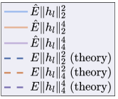
Refer to caption
Refer to caption
Refer to caption
Figure 22: Numerical validation of Theorem 17 using the classical stabilizing initializations (Glorot & Bengio, 2010; He et al., 2015). The variance of the weights is set to 1/d1𝑑1/\sqrt{d} for linear nets and 2/d2𝑑2/\sqrt{d} for ReLU nets (here, we used d=3,10𝑑310d=3,10). We consider a random Gaussian input and initialization of the weights with either Gaussian or uniform distribution. The theory matches the experiment (empirical mean denoted as 𝔼^^𝔼\hat{\mathbb{E}}1e51𝑒51e5 runs for d=10𝑑10d=10, 1e71𝑒71e7 runs for d=3𝑑3d=3). The results for the two initializations are similar, yet Gaussian case explodes a bit faster due to the effect of the kurtosis, which for the Gaussian is 333 while for the uniform is 3653653-\frac{6}{5}. The formula in Thm 17 also perfectly predicts this tiny shift in the population quantities, confirming the correctness of our calculations.

Simple take away.

Consider a Gaussian initialization κ=3𝜅3\kappa=3 in linear neural networks (p=1𝑝1p=1). Then the recursion matrix 𝐐𝐐{\bf Q} in Eq.(41) simplifies to

𝐐:=(d+2030),assign𝐐matrix𝑑2030\displaystyle{\bf Q}:=\begin{pmatrix}d+2&0\\ 3&0\end{pmatrix}, (46)

from which follows that 𝔼𝐖ϕk:1𝐳24=(dσ4)k(d+2)k𝔼𝐳42𝔼superscriptsubscriptnormsubscriptsuperscript𝐖:𝑘1italic-ϕ𝐳24superscript𝑑superscript𝜎4𝑘superscript𝑑2𝑘𝔼subscriptsuperscriptnorm𝐳24{\mathbb{E}}\|\mathbf{W}^{k:1}_{\phi}{\bf z}\|_{2}^{4}=\left(d\sigma^{4}\right)^{k}\left(d+2\right)^{k}{\mathbb{E}}\|{\bf z}\|^{2}_{4}. Hence, similar to the case of the neural chain depicted in Eq. 2 the pair of moments 𝔼𝐖ϕk:1𝐀𝐳22𝔼superscriptsubscriptnormsubscriptsuperscript𝐖:𝑘1italic-ϕ𝐀𝐳22{\mathbb{E}}\|\mathbf{W}^{k:1}_{\phi}{\bf A}{\bf z}\|_{2}^{2} and 𝔼𝐖ϕk:1𝐳24𝔼superscriptsubscriptnormsubscriptsuperscript𝐖:𝑘1italic-ϕ𝐳24{\mathbb{E}}\|\mathbf{W}^{k:1}_{\phi}{\bf z}\|_{2}^{4} cannot be stabilized jointly. Hence, as shown in Figure 20, the mean is allowed to be very different from the median by Mallows inequality Mallows & Richter (1969) — see also Thm. 9. Finally, we note that the effect we just discussed grows stronger if dLmuch-less-than𝑑𝐿d\ll L. This is also confirmed by the simulation in Figure 22.

Corollary 18 (Asymptotic forward pass statistics).
In the context of Theorem 17, as d𝑑d\to\infty 𝔼𝐖ϕk:1𝐀𝐱24(dσ2p)2k,less-than-or-similar-to𝔼superscriptsubscriptnormsubscriptsuperscript𝐖:𝑘1italic-ϕ𝐀𝐱24superscript𝑑superscript𝜎2𝑝2𝑘\displaystyle{\mathbb{E}}\|\mathbf{W}^{k:1}_{\phi}{\bf A}{\bf x}\|_{2}^{4}\lesssim(d\sigma^{2}p)^{2k}, (47) 𝔼𝐖ϕk:1𝐀𝐱44(dσ2p)2k,less-than-or-similar-to𝔼superscriptsubscriptnormsubscriptsuperscript𝐖:𝑘1italic-ϕ𝐀𝐱44superscript𝑑superscript𝜎2𝑝2𝑘\displaystyle{\mathbb{E}}\|\mathbf{W}^{k:1}_{\phi}{\bf A}{\bf x}\|_{4}^{4}\lesssim(d\sigma^{2}p)^{2k}, (48) where “less-than-or-similar-to\lesssim” denotes “asymptotically less of equal than a multiple of” (same as 𝒪𝒪\mathcal{O}).
Proof.

For the linear and the ReLU case we respectively have

𝐐linear=(d+2κ33κ3),𝐐ReLU=(d+2d+2κ432κ3).formulae-sequencesubscript𝐐linearmatrix𝑑2𝜅33𝜅3subscript𝐐ReLUmatrix𝑑2𝑑2𝜅432𝜅3{\bf Q}_{\text{linear}}=\begin{pmatrix}d+2&\kappa-3\\ 3&\kappa-3\end{pmatrix},\quad{\bf Q}_{\text{ReLU}}=\begin{pmatrix}d+2&d+2\kappa-4\\ 3&2\kappa-3\end{pmatrix}. (49)

As d𝑑d\to\infty, these matrices behave as follows:

𝐐linear=(𝒪(d)𝒪(1)𝒪(1)𝒪(1)),𝐐ReLU=(𝒪(d)𝒪(d)𝒪(1)𝒪(1)).formulae-sequencesubscriptsuperscript𝐐linearmatrix𝒪𝑑𝒪1𝒪1𝒪1subscriptsuperscript𝐐ReLUmatrix𝒪𝑑𝒪𝑑𝒪1𝒪1{\bf Q}^{\infty}_{\text{linear}}=\begin{pmatrix}\mathcal{O}(d)&\mathcal{O}(1)\\ \mathcal{O}(1)&\mathcal{O}(1)\end{pmatrix},\quad{\bf Q}^{\infty}_{\text{ReLU}}=\begin{pmatrix}\mathcal{O}(d)&\mathcal{O}(d)\\ \mathcal{O}(1)&\mathcal{O}(1)\end{pmatrix}. (50)

The result follows. ∎

Proposition 19 (Forward pass form a different vector).
Assume that, instead of 𝐱𝐱{\bf x}, we feed into the random net (with activation gates computed using 𝐱𝐱{\bf x}) a different vector 𝛂𝛂{\boldsymbol{\alpha}}. Then, all the forward pass statistics still hold.
Proof.

Direct consequence of Corollary 14, when applied iteratively as done above. ∎

Statistics for network-dependent matrices from the forward pass

Proposition 20 (From network matrices to propagations of canonical vectors).
Let 𝐞1subscript𝐞1{\bf e}_{1} be the first vector in the canonical basis. We have 𝔼𝐖ϕ:k+1F2=d𝔼𝐖ϕ:k+1𝐞122(dσ2p)k;𝔼subscriptsuperscriptnormsubscriptsuperscript𝐖:𝑘1italic-ϕ2𝐹𝑑𝔼subscriptsuperscriptnormsubscriptsuperscript𝐖:𝑘1italic-ϕsubscript𝐞122similar-tosuperscript𝑑superscript𝜎2𝑝𝑘\displaystyle{\mathbb{E}}\|\mathbf{W}^{\ell:k+1}_{\phi}\|^{2}_{F}=d\ {\mathbb{E}}\|\mathbf{W}^{\ell:k+1}_{\phi}{\bf e}_{1}\|^{2}_{2}\sim(d\sigma^{2}p)^{\ell-k}; (51) 𝔼𝐖ϕ:k+1F4=d2𝔼𝐖ϕ:k+1𝐞124(dσ2p)2(k).𝔼subscriptsuperscriptnormsubscriptsuperscript𝐖:𝑘1italic-ϕ4𝐹superscript𝑑2𝔼subscriptsuperscriptnormsubscriptsuperscript𝐖:𝑘1italic-ϕsubscript𝐞142similar-tosuperscript𝑑superscript𝜎2𝑝2𝑘\displaystyle{\mathbb{E}}\|\mathbf{W}^{\ell:k+1}_{\phi}\|^{4}_{F}=d^{2}\ {\mathbb{E}}\|\mathbf{W}^{\ell:k+1}_{\phi}{\bf e}_{1}\|^{4}_{2}\sim(d\sigma^{2}p)^{2(\ell-k)}. (52) where “less-than-or-similar-to\lesssim” denotes “asymptotically less of equal than a multiple of” (same as 𝒪𝒪\mathcal{O}).
Proof.

By direct calculation

𝔼𝐖ϕ:k+1F2=𝔼[i=1d𝐖ϕ:k+1𝐞i22]=d𝔼𝐖ϕ:k+1𝐞122(dσ2p)k.𝔼subscriptsuperscriptnormsubscriptsuperscript𝐖:𝑘1italic-ϕ2𝐹𝔼delimited-[]superscriptsubscript𝑖1𝑑subscriptsuperscriptnormsubscriptsuperscript𝐖:𝑘1italic-ϕsubscript𝐞𝑖22𝑑𝔼subscriptsuperscriptnormsubscriptsuperscript𝐖:𝑘1italic-ϕsubscript𝐞122similar-tosuperscript𝑑superscript𝜎2𝑝𝑘\displaystyle{\mathbb{E}}\|\mathbf{W}^{\ell:k+1}_{\phi}\|^{2}_{F}={\mathbb{E}}\left[\sum_{i=1}^{d}\|\mathbf{W}^{\ell:k+1}_{\phi}{\bf e}_{i}\|^{2}_{2}\right]=d\ {\mathbb{E}}\|\mathbf{W}^{\ell:k+1}_{\phi}{\bf e}_{1}\|^{2}_{2}\sim(d\sigma^{2}p)^{\ell-k}. (53)

The second last equality follows from the isotropic structure of 𝐖ϕ:ksubscriptsuperscript𝐖:𝑘italic-ϕ\mathbf{W}^{\ell:k}_{\phi} and the last from Prop. 19.

𝔼𝐖ϕ:k+1F4=𝔼[(i=1d𝐖ϕ:k+1𝐞i22)2]=𝔼[ij𝐖ϕ:k+1𝐞i22𝐖ϕ:k+1𝐞j22].𝔼subscriptsuperscriptnormsubscriptsuperscript𝐖:𝑘1italic-ϕ4𝐹𝔼delimited-[]superscriptsuperscriptsubscript𝑖1𝑑subscriptsuperscriptnormsubscriptsuperscript𝐖:𝑘1italic-ϕsubscript𝐞𝑖222𝔼delimited-[]subscript𝑖𝑗subscriptsuperscriptnormsubscriptsuperscript𝐖:𝑘1italic-ϕsubscript𝐞𝑖22subscriptsuperscriptnormsubscriptsuperscript𝐖:𝑘1italic-ϕsubscript𝐞𝑗22\displaystyle{\mathbb{E}}\|\mathbf{W}^{\ell:k+1}_{\phi}\|^{4}_{F}={\mathbb{E}}\left[\left(\sum_{i=1}^{d}\|\mathbf{W}^{\ell:k+1}_{\phi}{\bf e}_{i}\|^{2}_{2}\right)^{2}\right]={\mathbb{E}}\left[\sum_{ij}\|\mathbf{W}^{\ell:k+1}_{\phi}{\bf e}_{i}\|^{2}_{2}\|\mathbf{W}^{\ell:k+1}_{\phi}{\bf e}_{j}\|^{2}_{2}\right]. (54)

Since 𝐖ϕ:k+1𝐞j22=𝐖ϕ:k+1𝐞i22subscriptsuperscriptnormsubscriptsuperscript𝐖:𝑘1italic-ϕsubscript𝐞𝑗22subscriptsuperscriptnormsubscriptsuperscript𝐖:𝑘1italic-ϕsubscript𝐞𝑖22\|\mathbf{W}^{\ell:k+1}_{\phi}{\bf e}_{j}\|^{2}_{2}=\|\mathbf{W}^{\ell:k+1}_{\phi}{\bf e}_{i}\|^{2}_{2} in distribution, 𝔼𝐖ϕ:k+1F4=d2𝔼𝐖ϕ:k+1𝐞i24𝔼subscriptsuperscriptnormsubscriptsuperscript𝐖:𝑘1italic-ϕ4𝐹superscript𝑑2𝔼subscriptsuperscriptnormsubscriptsuperscript𝐖:𝑘1italic-ϕsubscript𝐞𝑖42{\mathbb{E}}\|\mathbf{W}^{\ell:k+1}_{\phi}\|^{4}_{F}=d^{2}{\mathbb{E}}\|\mathbf{W}^{\ell:k+1}_{\phi}{\bf e}_{i}\|^{4}_{2}. The asymptotic statements hold thanks to Proposition 19. ∎

B.3 Gradient

We consider the loss

𝐱,𝐲(𝐖)=12𝐲𝐁𝐃L𝐖ϕL:1𝐀𝐱2.subscript𝐱𝐲𝐖12superscriptnorm𝐲superscript𝐁𝐃𝐿subscriptsuperscript𝐖:𝐿1italic-ϕ𝐀𝐱2\displaystyle{\mathcal{L}}_{{\bf x},{\bf y}}({\bf W})=\frac{1}{2}\|{\bf y}-{\bf B}{\bf D}^{L}\mathbf{W}^{L:1}_{\phi}{\bf A}{\bf x}\|^{2}. (55)

As in (Allen-Zhu et al., 2019), by noting 𝐁~:=𝐁𝐃Lassign~𝐁superscript𝐁𝐃𝐿\tilde{\bf B}:={\bf B}{\bf D}^{L} and 𝐳=𝐀𝐱𝐳𝐀𝐱{\bf z}={\bf A}{\bf x} we get

𝐖ksuperscript𝐖𝑘\displaystyle\frac{\partial{\mathcal{L}}}{\partial\mathbf{W}^{k}} =𝐖ϕk+1:L𝐁~[𝐁~𝐖ϕL:1𝐳𝐲]𝐳𝐖1:k1absentsubscriptsuperscript𝐖:𝑘1𝐿italic-ϕsuperscript~𝐁topdelimited-[]~𝐁subscriptsuperscript𝐖:𝐿1italic-ϕ𝐳𝐲superscript𝐳topsuperscript𝐖:1𝑘1\displaystyle=\mathbf{W}^{k+1:L}_{\phi}\tilde{\bf B}^{\top}[\tilde{\bf B}\mathbf{W}^{L:1}_{\phi}{\bf z}-{\bf y}]{\bf z}^{\top}\mathbf{W}^{1:k-1} (56)
=𝐖ϕk+1:L𝐁~𝐁~𝐖ϕL:1𝐳𝐳𝐖1:k1k1𝐖ϕk+1:L𝐁~𝐲𝐳𝐖1:k1k2,absentsubscriptsubscriptsuperscript𝐖:𝑘1𝐿italic-ϕsuperscript~𝐁top~𝐁subscriptsuperscript𝐖:𝐿1italic-ϕsuperscript𝐳𝐳topsuperscript𝐖:1𝑘1superscriptsubscript𝑘1subscriptsubscriptsuperscript𝐖:𝑘1𝐿italic-ϕsuperscript~𝐁topsuperscript𝐲𝐳topsuperscript𝐖:1𝑘1superscriptsubscript𝑘2\displaystyle=\underbrace{\mathbf{W}^{k+1:L}_{\phi}\tilde{\bf B}^{\top}\tilde{\bf B}\mathbf{W}^{L:1}_{\phi}{\bf z}{\bf z}^{\top}\mathbf{W}^{1:k-1}}_{\boldsymbol{\partial}{\mathcal{L}}_{k}^{1}}-\underbrace{\mathbf{W}^{k+1:L}_{\phi}\tilde{\bf B}^{\top}{\bf y}{\bf z}^{\top}\mathbf{W}^{1:k-1}}_{\boldsymbol{\partial}{\mathcal{L}}_{k}^{2}}, (57)

with 𝐖ϕk+1:L:=(𝐖ϕL:k+1)assignsubscriptsuperscript𝐖:𝑘1𝐿italic-ϕsuperscriptsubscriptsuperscript𝐖:𝐿𝑘1italic-ϕtop\mathbf{W}^{k+1:L}_{\phi}:=\left(\mathbf{W}^{L:k+1}_{\phi}\right)^{\top}. By the triangle inequality, we have

𝐖kFk1F+k2F,subscriptnormsuperscript𝐖𝑘𝐹subscriptnormsuperscriptsubscript𝑘1𝐹subscriptnormsuperscriptsubscript𝑘2𝐹\displaystyle\left\|\frac{\partial{\mathcal{L}}}{\partial\mathbf{W}^{k}}\right\|_{F}\leq\|\boldsymbol{\partial}{\mathcal{L}}_{k}^{1}\|_{F}+\|\boldsymbol{\partial}{\mathcal{L}}_{k}^{2}\|_{F}, (58)

therefore we can bound each term individually. Let 𝔼p[]superscript𝔼𝑝delimited-[]{\mathbb{E}}^{p}[\cdot] be the p𝑝p-th power of 𝔼[]𝔼delimited-[]{\mathbb{E}}[\cdot].

Proposition 21 (Bounding gradients with forward passes).
We have 𝔼k1F𝔼subscriptnormsuperscriptsubscript𝑘1𝐹\displaystyle{\mathbb{E}}\|\boldsymbol{\partial}{\mathcal{L}}_{k}^{1}\|_{F} 𝔼1/2[𝐁~𝐖ϕL:k+122]𝔼1/4[𝐁~𝐖ϕL:1𝐳24]𝔼1/4[𝐖ϕk1:1𝐳24];absentsuperscript𝔼12delimited-[]subscriptsuperscriptnorm~𝐁subscriptsuperscript𝐖:𝐿𝑘1italic-ϕ22superscript𝔼14delimited-[]subscriptsuperscriptnorm~𝐁subscriptsuperscript𝐖:𝐿1italic-ϕ𝐳42superscript𝔼14delimited-[]subscriptsuperscriptnormsubscriptsuperscript𝐖:𝑘11italic-ϕ𝐳42\displaystyle\leq{\mathbb{E}}^{1/2}\left[\|\tilde{\bf B}\mathbf{W}^{L:k+1}_{\phi}\|^{2}_{2}\right]{\mathbb{E}}^{1/4}\left[\|\tilde{\bf B}\mathbf{W}^{L:1}_{\phi}{\bf z}\|^{4}_{2}\right]{\mathbb{E}}^{1/4}\left[\|\mathbf{W}^{k-1:1}_{\phi}{\bf z}\|^{4}_{2}\right]; (59) 𝔼k2F𝔼subscriptnormsuperscriptsubscript𝑘2𝐹\displaystyle{\mathbb{E}}\|\boldsymbol{\partial}{\mathcal{L}}_{k}^{2}\|_{F} 𝔼[𝐲𝐁~𝐖ϕL:k+122]𝔼[𝐖ϕk1:1𝐳22].absent𝔼delimited-[]subscriptsuperscriptnormsuperscript𝐲top~𝐁subscriptsuperscript𝐖:𝐿𝑘1italic-ϕ22𝔼delimited-[]subscriptsuperscriptnormsubscriptsuperscript𝐖:𝑘11italic-ϕ𝐳22\displaystyle\leq{\mathbb{E}}\left[\|{\bf y}^{\top}\tilde{\bf B}\mathbf{W}^{L:k+1}_{\phi}\|^{2}_{2}\right]{\mathbb{E}}\left[\|\mathbf{W}^{k-1:1}_{\phi}{\bf z}\|^{2}_{2}\right]. (60)
Proof.

The bounds follow from submultiplicativity of Frobenius norm and Cauchy-Schwarz inequality — applied possibly twice.

𝔼k1F𝔼subscriptnormsuperscriptsubscript𝑘1𝐹\displaystyle{\mathbb{E}}\|\boldsymbol{\partial}{\mathcal{L}}_{k}^{1}\|_{F} =𝔼𝐖ϕk+1:L𝐁~𝐁~𝐖ϕL:1𝐳𝐳𝐖ϕ1:k1Fabsent𝔼subscriptnormsubscriptsuperscript𝐖:𝑘1𝐿italic-ϕsuperscript~𝐁top~𝐁subscriptsuperscript𝐖:𝐿1italic-ϕsuperscript𝐳𝐳topsubscriptsuperscript𝐖:1𝑘1italic-ϕ𝐹\displaystyle={\mathbb{E}}\|\mathbf{W}^{k+1:L}_{\phi}\tilde{\bf B}^{\top}\tilde{\bf B}\mathbf{W}^{L:1}_{\phi}{\bf z}{\bf z}^{\top}\mathbf{W}^{1:k-1}_{\phi}\|_{F} (61)
𝔼[𝐖ϕk+1:L𝐁~F𝐁~𝐖ϕL:1𝐳F𝐳𝐖ϕ1:k1F]absent𝔼delimited-[]subscriptnormsubscriptsuperscript𝐖:𝑘1𝐿italic-ϕsuperscript~𝐁top𝐹subscriptnorm~𝐁subscriptsuperscript𝐖:𝐿1italic-ϕ𝐳𝐹subscriptnormsuperscript𝐳topsubscriptsuperscript𝐖:1𝑘1italic-ϕ𝐹\displaystyle\leq{\mathbb{E}}\left[\|\mathbf{W}^{k+1:L}_{\phi}\tilde{\bf B}^{\top}\|_{F}\|\tilde{\bf B}\mathbf{W}^{L:1}_{\phi}{\bf z}\|_{F}\|{\bf z}^{\top}\mathbf{W}^{1:k-1}_{\phi}\|_{F}\right] (62)
=𝔼[𝐁~𝐖ϕL:k+1F𝐁~𝐖ϕL:1𝐳F𝐖ϕk1:1𝐳F]absent𝔼delimited-[]subscriptnorm~𝐁subscriptsuperscript𝐖:𝐿𝑘1italic-ϕ𝐹subscriptnorm~𝐁subscriptsuperscript𝐖:𝐿1italic-ϕ𝐳𝐹subscriptnormsubscriptsuperscript𝐖:𝑘11italic-ϕ𝐳𝐹\displaystyle={\mathbb{E}}\left[\|\tilde{\bf B}\mathbf{W}^{L:k+1}_{\phi}\|_{F}\|\tilde{\bf B}\mathbf{W}^{L:1}_{\phi}{\bf z}\|_{F}\|\mathbf{W}^{k-1:1}_{\phi}{\bf z}\|_{F}\right] (63)
𝔼1/2[𝐁~𝐖ϕL:k+1F2]𝔼1/2[𝐁~𝐖ϕL:1𝐳F2𝐖ϕk1:1𝐳F2]absentsuperscript𝔼12delimited-[]subscriptsuperscriptnorm~𝐁subscriptsuperscript𝐖:𝐿𝑘1italic-ϕ2𝐹superscript𝔼12delimited-[]subscriptsuperscriptnorm~𝐁subscriptsuperscript𝐖:𝐿1italic-ϕ𝐳2𝐹subscriptsuperscriptnormsubscriptsuperscript𝐖:𝑘11italic-ϕ𝐳2𝐹\displaystyle\leq{\mathbb{E}}^{1/2}\left[\|\tilde{\bf B}\mathbf{W}^{L:k+1}_{\phi}\|^{2}_{F}\right]{\mathbb{E}}^{1/2}\left[\|\tilde{\bf B}\mathbf{W}^{L:1}_{\phi}{\bf z}\|^{2}_{F}\|\mathbf{W}^{k-1:1}_{\phi}{\bf z}\|^{2}_{F}\right] (64)
𝔼1/2[𝐁~𝐖ϕL:k+1F2]𝔼1/4[𝐁~𝐖ϕL:1𝐳F4]𝔼1/4[𝐖ϕk1:1𝐳F4].absentsuperscript𝔼12delimited-[]subscriptsuperscriptnorm~𝐁subscriptsuperscript𝐖:𝐿𝑘1italic-ϕ2𝐹superscript𝔼14delimited-[]subscriptsuperscriptnorm~𝐁subscriptsuperscript𝐖:𝐿1italic-ϕ𝐳4𝐹superscript𝔼14delimited-[]subscriptsuperscriptnormsubscriptsuperscript𝐖:𝑘11italic-ϕ𝐳4𝐹\displaystyle\leq{\mathbb{E}}^{1/2}\left[\|\tilde{\bf B}\mathbf{W}^{L:k+1}_{\phi}\|^{2}_{F}\right]{\mathbb{E}}^{1/4}\left[\|\tilde{\bf B}\mathbf{W}^{L:1}_{\phi}{\bf z}\|^{4}_{F}\right]{\mathbb{E}}^{1/4}\left[\|\mathbf{W}^{k-1:1}_{\phi}{\bf z}\|^{4}_{F}\right]. (65)
𝔼k2F𝔼subscriptnormsuperscriptsubscript𝑘2𝐹\displaystyle{\mathbb{E}}\|\boldsymbol{\partial}{\mathcal{L}}_{k}^{2}\|_{F} =𝔼𝐖ϕk+1:L𝐁~𝐲𝐳𝐖ϕ1:k1Fabsent𝔼subscriptnormsubscriptsuperscript𝐖:𝑘1𝐿italic-ϕsuperscript~𝐁topsuperscript𝐲𝐳topsubscriptsuperscript𝐖:1𝑘1italic-ϕ𝐹\displaystyle={\mathbb{E}}\|\mathbf{W}^{k+1:L}_{\phi}\tilde{\bf B}^{\top}{\bf y}{\bf z}^{\top}\mathbf{W}^{1:k-1}_{\phi}\|_{F} (66)
𝔼[𝐖ϕk+1:L𝐁~𝐲F𝐳𝐖ϕ1:k1F]absent𝔼delimited-[]subscriptnormsubscriptsuperscript𝐖:𝑘1𝐿italic-ϕsuperscript~𝐁top𝐲𝐹subscriptnormsuperscript𝐳topsubscriptsuperscript𝐖:1𝑘1italic-ϕ𝐹\displaystyle\leq{\mathbb{E}}\left[\|\mathbf{W}^{k+1:L}_{\phi}\tilde{\bf B}^{\top}{\bf y}\|_{F}\|{\bf z}^{\top}\mathbf{W}^{1:k-1}_{\phi}\|_{F}\right] (67)
𝔼1/2[𝐖ϕk+1:L𝐁~𝐲F2]𝔼1/2[𝐳𝐖ϕ1:k1F2]absentsuperscript𝔼12delimited-[]subscriptsuperscriptnormsubscriptsuperscript𝐖:𝑘1𝐿italic-ϕsuperscript~𝐁top𝐲2𝐹superscript𝔼12delimited-[]subscriptsuperscriptnormsuperscript𝐳topsubscriptsuperscript𝐖:1𝑘1italic-ϕ2𝐹\displaystyle\leq{\mathbb{E}}^{1/2}\left[\|\mathbf{W}^{k+1:L}_{\phi}\tilde{\bf B}^{\top}{\bf y}\|^{2}_{F}\right]{\mathbb{E}}^{1/2}\left[\|{\bf z}^{\top}\mathbf{W}^{1:k-1}_{\phi}\|^{2}_{F}\right] (68)
=𝔼1/2[𝐲𝐁~𝐖ϕL:k+1F2]𝔼1/2[𝐖ϕk1:1𝐳F2].absentsuperscript𝔼12delimited-[]subscriptsuperscriptnormsuperscript𝐲top~𝐁subscriptsuperscript𝐖:𝐿𝑘1italic-ϕ2𝐹superscript𝔼12delimited-[]subscriptsuperscriptnormsubscriptsuperscript𝐖:𝑘11italic-ϕ𝐳2𝐹\displaystyle={\mathbb{E}}^{1/2}\left[\|{\bf y}^{\top}\tilde{\bf B}\mathbf{W}^{L:k+1}_{\phi}\|^{2}_{F}\right]{\mathbb{E}}^{1/2}\left[\|\mathbf{W}^{k-1:1}_{\phi}{\bf z}\|^{2}_{F}\right]. (69)

We conclude by noting that the Frobenius norm is the 222-norm for vectors. ∎

Proposition 22 (Bounding gradients with forward passes, wide net).
As d𝑑d\to\infty, 𝔼k1F𝔼subscriptnormsuperscriptsubscript𝑘1𝐹\displaystyle{\mathbb{E}}\|\boldsymbol{\partial}{\mathcal{L}}_{k}^{1}\|_{F} (pσ2d)2L12,less-than-or-similar-toabsentsuperscript𝑝superscript𝜎2𝑑2𝐿12\displaystyle\lesssim(p\sigma^{2}d)^{\frac{2L-1}{2}}, (70) 𝔼k2F𝔼subscriptnormsuperscriptsubscript𝑘2𝐹\displaystyle{\mathbb{E}}\|\boldsymbol{\partial}{\mathcal{L}}_{k}^{2}\|_{F} (pσ2d)L12,less-than-or-similar-toabsentsuperscript𝑝superscript𝜎2𝑑𝐿12\displaystyle\lesssim(p\sigma^{2}d)^{\frac{L-1}{2}}, (71) where “less-than-or-similar-to\lesssim” denotes “asymptotically less of equal than a multiple of” (same as 𝒪𝒪\mathcal{O}). Hence, we have 𝔼𝐖kF𝔼subscriptnormsuperscript𝐖𝑘𝐹\displaystyle{\mathbb{E}}\left\|\frac{\partial{\mathcal{L}}}{\partial\mathbf{W}^{k}}\right\|_{F} (pσ2d)L12if (pσ2d)1(vanishing-stable regime).formulae-sequenceless-than-or-similar-toabsentsuperscript𝑝superscript𝜎2𝑑𝐿12if 𝑝superscript𝜎2𝑑1(vanishing-stable regime)\displaystyle\lesssim(p\sigma^{2}d)^{\frac{L-1}{2}}\quad\quad\text{if }\quad(p\sigma^{2}d)\leq 1\quad\text{(vanishing-stable regime)}. (72) 𝔼𝐖kF𝔼subscriptnormsuperscript𝐖𝑘𝐹\displaystyle{\mathbb{E}}\left\|\frac{\partial{\mathcal{L}}}{\partial\mathbf{W}^{k}}\right\|_{F} (pσ2d)2L12if (pσ2d)1(exploding regime).formulae-sequenceless-than-or-similar-toabsentsuperscript𝑝superscript𝜎2𝑑2𝐿12if 𝑝superscript𝜎2𝑑1(exploding regime)\displaystyle\lesssim(p\sigma^{2}d)^{\frac{2L-1}{2}}\quad\quad\text{if }\quad(p\sigma^{2}d)\geq 1\quad\text{(exploding regime)}. (73)
Proof.

Simple application of Corollary 18 and Proposition 20 to the bounds in Proposition 21. ∎

B.4 Hessian

The Hessian of a linear DNN can be split into two block matrices, where each block has a Kronecker product structure. We can apply the product rule to the gradient and consider 𝐖superscript𝐖\mathbf{W}^{\ell} and 𝐖superscript𝐖limit-fromtop\mathbf{W}^{\ell\top} (>k𝑘\ell>k) as two distinct matrices: the block (k,)𝑘(k,\ell) of the Hessian matrix is:

2𝐖k𝐖𝐇1k+2𝐖k𝐖𝐇2k(𝐖)𝐖𝕋,subscriptsuperscript2superscript𝐖𝑘superscript𝐖subscriptsuperscript𝐇𝑘1subscriptsuperscript2superscript𝐖𝑘superscript𝐖limit-fromtopsubscriptsuperscript𝐇𝑘2subscriptsuperscript𝐖limit-fromtopsuperscript𝐖𝕋\underbrace{\frac{\partial^{2}{\mathcal{L}}}{\partial\mathbf{W}^{k}\partial\mathbf{W}^{\ell}}}_{\mathbf{H}^{k\ell}_{1}}+\underbrace{\frac{\partial^{2}{\mathcal{L}}}{\partial\mathbf{W}^{k}{\partial\mathbf{W}^{\ell\top}}}}_{\mathbf{H}^{k\ell}_{2}}\underbrace{\frac{\partial(\mathbf{W}^{\ell\top})}{\partial\mathbf{W}^{\ell}}}_{\mathbb{T}},

where 𝕋𝕋\mathbb{T} is the matrix transpose tensor. Recall that

𝐖k=𝐖ϕk+1:L𝐁~[𝐁~𝐖ϕL:1𝐳𝐲]𝐳𝐖1:k1.superscript𝐖𝑘subscriptsuperscript𝐖:𝑘1𝐿italic-ϕsuperscript~𝐁topdelimited-[]~𝐁subscriptsuperscript𝐖:𝐿1italic-ϕ𝐳𝐲superscript𝐳topsuperscript𝐖:1𝑘1\displaystyle\frac{\partial{\mathcal{L}}}{\partial\mathbf{W}^{k}}=\mathbf{W}^{k+1:L}_{\phi}\tilde{\bf B}^{\top}[\tilde{\bf B}\mathbf{W}^{L:1}_{\phi}{\bf z}-{\bf y}]{\bf z}^{\top}\mathbf{W}^{1:k-1}. (74)

By using the simple rule 𝐄𝐖𝐅𝐖=𝐅𝐄𝐄𝐖𝐅𝐖tensor-productsuperscript𝐅top𝐄\frac{\partial\mathbf{E}{\bf W}\mathbf{F}}{\partial{\bf W}}=\mathbf{F}^{\top}\otimes\mathbf{E}, we get

𝐇1ksubscriptsuperscript𝐇𝑘1\displaystyle\mathbf{H}^{k\ell}_{1} =𝐖ϕk1:1𝐳𝐳𝐖ϕ1:1𝐖ϕk+1:L𝐁~𝐁~𝐖ϕL:+1;absenttensor-productsubscriptsuperscript𝐖:𝑘11italic-ϕsuperscript𝐳𝐳topsubscriptsuperscript𝐖:11italic-ϕsubscriptsuperscript𝐖:𝑘1𝐿italic-ϕsuperscript~𝐁top~𝐁subscriptsuperscript𝐖:𝐿1italic-ϕ\displaystyle=\mathbf{W}^{k-1:1}_{\phi}{\bf z}{\bf z}^{\top}\mathbf{W}^{1:\ell-1}_{\phi}\;\otimes\;\mathbf{W}^{k+1:L}_{\phi}\tilde{\bf B}^{\top}\tilde{\bf B}\mathbf{W}^{L:\ell+1}_{\phi}; (75)
𝐇2ksubscriptsuperscript𝐇𝑘2\displaystyle\mathbf{H}^{k\ell}_{2} =𝐖ϕk1:1𝐳(𝐳𝐖ϕ1:L𝐁~𝐲)𝐁~𝐖ϕL:+1𝐖ϕk+1:1absenttensor-productsubscriptsuperscript𝐖:𝑘11italic-ϕ𝐳superscript𝐳topsubscriptsuperscript𝐖:1𝐿italic-ϕsuperscript~𝐁topsuperscript𝐲top~𝐁subscriptsuperscript𝐖:𝐿1italic-ϕsubscriptsuperscript𝐖:𝑘11italic-ϕ\displaystyle=\mathbf{W}^{k-1:1}_{\phi}{\bf z}\left({\bf z}^{\top}\mathbf{W}^{1:L}_{\phi}\tilde{\bf B}^{\top}-{\bf y}^{\top}\right)\tilde{\bf B}\mathbf{W}^{L:\ell+1}_{\phi}\otimes\mathbf{W}^{k+1:\ell-1}_{\phi} (76)
=𝐖ϕk1:1𝐳𝐳𝐖ϕ1:L𝐁~𝐁~𝐖ϕL:+1𝐖ϕk+1:1𝐇21k𝐖ϕk1:1𝐳𝐲𝐁~𝐖ϕL:+1𝐖ϕk+1:1𝐇22k,absentsubscripttensor-productsubscriptsuperscript𝐖:𝑘11italic-ϕsuperscript𝐳𝐳topsubscriptsuperscript𝐖:1𝐿italic-ϕsuperscript~𝐁top~𝐁subscriptsuperscript𝐖:𝐿1italic-ϕsubscriptsuperscript𝐖:𝑘11italic-ϕsubscriptsuperscript𝐇𝑘21subscripttensor-productsubscriptsuperscript𝐖:𝑘11italic-ϕsuperscript𝐳𝐲top~𝐁subscriptsuperscript𝐖:𝐿1italic-ϕsubscriptsuperscript𝐖:𝑘11italic-ϕsubscriptsuperscript𝐇𝑘22\displaystyle=\underbrace{\mathbf{W}^{k-1:1}_{\phi}{\bf z}{\bf z}^{\top}\mathbf{W}^{1:L}_{\phi}\tilde{\bf B}^{\top}\tilde{\bf B}\mathbf{W}^{L:\ell+1}_{\phi}\otimes\mathbf{W}^{k+1:\ell-1}_{\phi}}_{\mathbf{H}^{k\ell}_{21}}-\underbrace{\mathbf{W}^{k-1:1}_{\phi}{\bf z}{\bf y}^{\top}\tilde{\bf B}\mathbf{W}^{L:\ell+1}_{\phi}\otimes\mathbf{W}^{k+1:\ell-1}_{\phi}}_{\mathbf{H}^{k\ell}_{22}},

Note that if instead k=𝑘k=\ell, 𝐇kk=𝐇1kksuperscript𝐇𝑘𝑘subscriptsuperscript𝐇𝑘𝑘1\mathbf{H}^{kk}=\mathbf{H}^{kk}_{1}.

Proposition 23 (Bounding the Hessian with forward passes).
It is possible to bound the Hessian with statistics only on the forward pass.
Proof.

We simply apply the Cauchy-Schwarz inequality twice for each term, using also the Frobenius norm formula for the Kronecker product and norm submultiplicativity.

𝔼𝐇1kF𝔼subscriptnormsubscriptsuperscript𝐇𝑘1𝐹\displaystyle{\mathbb{E}}\|\mathbf{H}^{k\ell}_{1}\|_{F} =𝔼𝐖ϕk1:1𝐳𝐳𝐖ϕ1:1𝐖ϕk+1:L𝐁~𝐁~𝐖ϕL:+1Fabsent𝔼subscriptnormtensor-productsubscriptsuperscript𝐖:𝑘11italic-ϕsuperscript𝐳𝐳topsubscriptsuperscript𝐖:11italic-ϕsubscriptsuperscript𝐖:𝑘1𝐿italic-ϕsuperscript~𝐁top~𝐁subscriptsuperscript𝐖:𝐿1italic-ϕ𝐹\displaystyle={\mathbb{E}}\left\|\mathbf{W}^{k-1:1}_{\phi}{\bf z}{\bf z}^{\top}\mathbf{W}^{1:\ell-1}_{\phi}\;\otimes\;\mathbf{W}^{k+1:L}_{\phi}\tilde{\bf B}^{\top}\tilde{\bf B}\mathbf{W}^{L:\ell+1}_{\phi}\right\|_{F} (77)
𝔼1/2𝐖ϕk1:1𝐳𝐳𝐖ϕ1:1F2𝔼1/2𝐖ϕk+1:L𝐁~𝐁~𝐖ϕL:+1F2absentsuperscript𝔼12subscriptsuperscriptnormsubscriptsuperscript𝐖:𝑘11italic-ϕsuperscript𝐳𝐳topsubscriptsuperscript𝐖:11italic-ϕ2𝐹superscript𝔼12subscriptsuperscriptnormsubscriptsuperscript𝐖:𝑘1𝐿italic-ϕsuperscript~𝐁top~𝐁subscriptsuperscript𝐖:𝐿1italic-ϕ2𝐹\displaystyle\leq{\mathbb{E}}^{1/2}\left\|\mathbf{W}^{k-1:1}_{\phi}{\bf z}{\bf z}^{\top}\mathbf{W}^{1:\ell-1}_{\phi}\right\|^{2}_{F}{\mathbb{E}}^{1/2}\left\|\mathbf{W}^{k+1:L}_{\phi}\tilde{\bf B}^{\top}\tilde{\bf B}\mathbf{W}^{L:\ell+1}_{\phi}\right\|^{2}_{F} (78)
𝔼1/4𝐖ϕk1:1𝐳F4𝔼1/4𝐖ϕ1:1𝐳F4𝔼1/4𝐁~𝐖ϕL:+1F4𝔼1/4𝐁~𝐖ϕL:k+1F4.absentsuperscript𝔼14subscriptsuperscriptnormsubscriptsuperscript𝐖:𝑘11italic-ϕ𝐳4𝐹superscript𝔼14subscriptsuperscriptnormsubscriptsuperscript𝐖:11italic-ϕ𝐳4𝐹superscript𝔼14subscriptsuperscriptnorm~𝐁subscriptsuperscript𝐖:𝐿1italic-ϕ4𝐹superscript𝔼14subscriptsuperscriptnorm~𝐁subscriptsuperscript𝐖:𝐿𝑘1italic-ϕ4𝐹\displaystyle\leq{\mathbb{E}}^{1/4}\left\|\mathbf{W}^{k-1:1}_{\phi}{\bf z}\right\|^{4}_{F}{\mathbb{E}}^{1/4}\left\|\mathbf{W}^{\ell-1:1}_{\phi}{\bf z}\right\|^{4}_{F}{\mathbb{E}}^{1/4}\left\|\tilde{\bf B}\mathbf{W}^{L:\ell+1}_{\phi}\right\|^{4}_{F}{\mathbb{E}}^{1/4}\left\|\tilde{\bf B}\mathbf{W}^{L:k+1}_{\phi}\right\|^{4}_{F}. (79)
𝔼𝐇22kF𝔼subscriptnormsubscriptsuperscript𝐇𝑘22𝐹\displaystyle{\mathbb{E}}\|\mathbf{H}^{k\ell}_{22}\|_{F} 𝔼1/2𝐖ϕk1:1𝐳𝐲𝐁~𝐖ϕL:+1F2𝔼1/2𝐖ϕk+1:1F2absentsuperscript𝔼12subscriptsuperscriptnormsubscriptsuperscript𝐖:𝑘11italic-ϕsuperscript𝐳𝐲top~𝐁subscriptsuperscript𝐖:𝐿1italic-ϕ2𝐹superscript𝔼12subscriptsuperscriptnormsubscriptsuperscript𝐖:𝑘11italic-ϕ2𝐹\displaystyle\leq{\mathbb{E}}^{1/2}\left\|\mathbf{W}^{k-1:1}_{\phi}{\bf z}{\bf y}^{\top}\tilde{\bf B}\mathbf{W}^{L:\ell+1}_{\phi}\right\|^{2}_{F}{\mathbb{E}}^{1/2}\left\|\mathbf{W}^{k+1:\ell-1}_{\phi}\right\|^{2}_{F} (80)
𝔼1/4𝐖ϕk1:1𝐳F4𝔼1/4𝐲𝐁~𝐖ϕL:+1F4𝔼1/2𝐖ϕ1:k+1F2.absentsuperscript𝔼14subscriptsuperscriptnormsubscriptsuperscript𝐖:𝑘11italic-ϕ𝐳4𝐹superscript𝔼14subscriptsuperscriptnormsuperscript𝐲top~𝐁subscriptsuperscript𝐖:𝐿1italic-ϕ4𝐹superscript𝔼12subscriptsuperscriptnormsubscriptsuperscript𝐖:1𝑘1italic-ϕ2𝐹\displaystyle\leq{\mathbb{E}}^{1/4}\left\|\mathbf{W}^{k-1:1}_{\phi}{\bf z}\right\|^{4}_{F}{\mathbb{E}}^{1/4}\left\|{\bf y}^{\top}\tilde{\bf B}\mathbf{W}^{L:\ell+1}_{\phi}\right\|^{4}_{F}{\mathbb{E}}^{1/2}\left\|\mathbf{W}^{\ell-1:k+1}_{\phi}\right\|^{2}_{F}. (81)
𝔼𝐇21kF𝔼subscriptnormsubscriptsuperscript𝐇𝑘21𝐹\displaystyle{\mathbb{E}}\|\mathbf{H}^{k\ell}_{21}\|_{F} 𝔼1/2𝐖ϕk1:1𝐳𝐳𝐖ϕ1:L𝐁~𝐁~𝐖ϕL:+1F2𝔼1/2𝐖ϕk+1:1F2absentsuperscript𝔼12subscriptsuperscriptnormsubscriptsuperscript𝐖:𝑘11italic-ϕsuperscript𝐳𝐳topsubscriptsuperscript𝐖:1𝐿italic-ϕsuperscript~𝐁top~𝐁subscriptsuperscript𝐖:𝐿1italic-ϕ2𝐹superscript𝔼12subscriptsuperscriptnormsubscriptsuperscript𝐖:𝑘11italic-ϕ2𝐹\displaystyle\leq{\mathbb{E}}^{1/2}\left\|\mathbf{W}^{k-1:1}_{\phi}{\bf z}{\bf z}^{\top}\mathbf{W}^{1:L}_{\phi}\tilde{\bf B}^{\top}\tilde{\bf B}\mathbf{W}^{L:\ell+1}_{\phi}\right\|^{2}_{F}{\mathbb{E}}^{1/2}\left\|\mathbf{W}^{k+1:\ell-1}_{\phi}\right\|^{2}_{F} (82)
𝔼1/4𝐖ϕk1:1𝐳𝐳𝐖ϕ1:𝐖ϕ+1:L𝐁~𝐁~𝐖ϕL:+1F2𝔼1/4𝐖ϕ1:k+1F2.absentsuperscript𝔼14subscriptsuperscriptnormsubscriptsuperscript𝐖:𝑘11italic-ϕsuperscript𝐳𝐳topsubscriptsuperscript𝐖:1italic-ϕsubscriptsuperscript𝐖:1𝐿italic-ϕsuperscript~𝐁top~𝐁subscriptsuperscript𝐖:𝐿1italic-ϕ2𝐹superscript𝔼14subscriptsuperscriptnormsubscriptsuperscript𝐖:1𝑘1italic-ϕ2𝐹\displaystyle\leq{\mathbb{E}}^{1/4}\left\|\mathbf{W}^{k-1:1}_{\phi}{\bf z}{\bf z}^{\top}\mathbf{W}^{1:\ell}_{\phi}\mathbf{W}^{\ell+1:L}_{\phi}\tilde{\bf B}^{\top}\tilde{\bf B}\mathbf{W}^{L:\ell+1}_{\phi}\right\|^{2}_{F}{\mathbb{E}}^{1/4}\left\|\mathbf{W}^{\ell-1:k+1}_{\phi}\right\|^{2}_{F}. (83)

Note that the last term is not simplified completely, but unfortunately a simple iterated Cauchy-Schwarz splitting would lead to quantities with high exponents (eighth moment). Hence, we need to take a more complex approach. First, we split between terms which do not share weights.

𝔼[𝐖ϕk1:1𝐳𝐳𝐖ϕ1:F2𝐖ϕ+1:L𝐁~𝐁~𝐖ϕL:+1F2].𝔼delimited-[]subscriptsuperscriptnormsubscriptsuperscript𝐖:𝑘11italic-ϕsuperscript𝐳𝐳topsubscriptsuperscript𝐖:1italic-ϕ2𝐹subscriptsuperscriptnormsubscriptsuperscript𝐖:1𝐿italic-ϕsuperscript~𝐁top~𝐁subscriptsuperscript𝐖:𝐿1italic-ϕ2𝐹\displaystyle{\mathbb{E}}\left[\left\|\mathbf{W}^{k-1:1}_{\phi}{\bf z}{\bf z}^{\top}\mathbf{W}^{1:\ell}_{\phi}\right\|^{2}_{F}\left\|\mathbf{W}^{\ell+1:L}_{\phi}\tilde{\bf B}^{\top}\tilde{\bf B}\mathbf{W}^{L:\ell+1}_{\phi}\right\|^{2}_{F}\right]. (84)

Using the law of total expectation, the last expression becomes

𝔼[𝔼[𝐖ϕk1:1𝐳𝐳𝐖ϕ1:F𝐖ϕ+1:L𝐁~𝐁~𝐖ϕL:+1F2|]],\displaystyle{\mathbb{E}}\left[\ \ {\mathbb{E}}\left[\ \ \left\|\mathbf{W}^{k-1:1}_{\phi}{\bf z}{\bf z}^{\top}\mathbf{W}^{1:\ell}_{\phi}\right\|_{F}\left\|\mathbf{W}^{\ell+1:L}_{\phi}\tilde{\bf B}^{\top}\tilde{\bf B}\mathbf{W}^{L:\ell+1}_{\phi}\right\|^{2}_{F}\ \ \bigg{\lvert}\ \ \mathcal{F}_{\ell}\ \ \right]\ \ \right], (85)

where subscript\mathcal{F}_{\ell} is the information until layer \ell. Using the same reasoning as Corollary 14 and Proposition 19, it is easy to realize that fixing the preactivation a separate integration of the second term in the product. In particular, the expression becomes

𝔼[𝐖ϕk1:1𝐳𝐳𝐖ϕ1:F]𝔼[𝐖ϕ+1:L𝐁~𝐁~𝐖ϕL:+1F2|].\displaystyle{\mathbb{E}}\left[\left\|\mathbf{W}^{k-1:1}_{\phi}{\bf z}{\bf z}^{\top}\mathbf{W}^{1:\ell}_{\phi}\right\|_{F}\right]\ \cdot\ {\mathbb{E}}\left[\ \ \left\|\mathbf{W}^{\ell+1:L}_{\phi}\tilde{\bf B}^{\top}\tilde{\bf B}\mathbf{W}^{L:\ell+1}_{\phi}\right\|^{2}_{F}\ \ \bigg{\lvert}\ \ \mathcal{F}_{\ell}\ \ \right]. (86)

As usual, we drop the filtration notation and plug this back into the expression for 𝔼𝐇21kF𝔼subscriptnormsubscriptsuperscript𝐇𝑘21𝐹{\mathbb{E}}\|\mathbf{H}^{k\ell}_{21}\|_{F}:

𝔼𝐇21kF𝔼subscriptnormsubscriptsuperscript𝐇𝑘21𝐹\displaystyle{\mathbb{E}}\|\mathbf{H}^{k\ell}_{21}\|_{F} 𝔼1/2𝐖ϕk1:1𝐳𝐳𝐖ϕ1:F2𝔼1/2𝐖ϕ+1:L𝐁~𝐁~𝐖ϕL:+1F2𝔼1/2𝐖ϕ1:k+1F2absentsuperscript𝔼12subscriptsuperscriptnormsubscriptsuperscript𝐖:𝑘11italic-ϕsuperscript𝐳𝐳topsubscriptsuperscript𝐖:1italic-ϕ2𝐹superscript𝔼12subscriptsuperscriptnormsubscriptsuperscript𝐖:1𝐿italic-ϕsuperscript~𝐁top~𝐁subscriptsuperscript𝐖:𝐿1italic-ϕ2𝐹superscript𝔼12subscriptsuperscriptnormsubscriptsuperscript𝐖:1𝑘1italic-ϕ2𝐹\displaystyle\leq{\mathbb{E}}^{1/2}\left\|\mathbf{W}^{k-1:1}_{\phi}{\bf z}{\bf z}^{\top}\mathbf{W}^{1:\ell}_{\phi}\right\|^{2}_{F}{\mathbb{E}}^{1/2}\left\|\mathbf{W}^{\ell+1:L}_{\phi}\tilde{\bf B}^{\top}\tilde{\bf B}\mathbf{W}^{L:\ell+1}_{\phi}\right\|^{2}_{F}{\mathbb{E}}^{1/2}\left\|\mathbf{W}^{\ell-1:k+1}_{\phi}\right\|^{2}_{F}
𝔼1/4𝐖ϕk1:1𝐳F4𝔼1/4𝐖ϕ:1𝐳F4+𝔼1/2𝐁~𝐖ϕL:+1F4𝔼1/2𝐖ϕ1:k+1F2.absentsuperscript𝔼14subscriptsuperscriptnormsubscriptsuperscript𝐖:𝑘11italic-ϕ𝐳4𝐹superscript𝔼14subscriptsuperscriptnormsubscriptsuperscript𝐖:1italic-ϕ𝐳4𝐹superscript𝔼12subscriptsuperscriptnorm~𝐁subscriptsuperscript𝐖:𝐿1italic-ϕ4𝐹superscript𝔼12subscriptsuperscriptnormsubscriptsuperscript𝐖:1𝑘1italic-ϕ2𝐹\displaystyle\leq{\mathbb{E}}^{1/4}\left\|\mathbf{W}^{k-1:1}_{\phi}{\bf z}\right\|^{4}_{F}{\mathbb{E}}^{1/4}\left\|\mathbf{W}^{\ell:1}_{\phi}{\bf z}\right\|^{4}_{F}+{\mathbb{E}}^{1/2}\left\|\tilde{\bf B}\mathbf{W}^{L:\ell+1}_{\phi}\right\|^{4}_{F}{\mathbb{E}}^{1/2}\left\|\mathbf{W}^{\ell-1:k+1}_{\phi}\right\|^{2}_{F}.

Proposition 24 (Bounding Hessians with forward passes, wide net).
As d𝑑d\to\infty, for k𝑘k\neq\ell 𝔼𝐇kF𝔼subscriptnormsuperscript𝐇𝑘𝐹\displaystyle{\mathbb{E}}\|\mathbf{H}^{k\ell}\|_{F} (pσ2d)L22+(pσ2d)L1,less-than-or-similar-toabsentsuperscript𝑝superscript𝜎2𝑑𝐿22superscript𝑝superscript𝜎2𝑑𝐿1\displaystyle\lesssim(p\sigma^{2}d)^{\frac{L-2}{2}}+(p\sigma^{2}d)^{L-1}, (87) 𝔼𝐇kkF𝔼subscriptnormsuperscript𝐇𝑘𝑘𝐹\displaystyle{\mathbb{E}}\|\mathbf{H}^{kk}\|_{F} (pσ2d)L1,less-than-or-similar-toabsentsuperscript𝑝superscript𝜎2𝑑𝐿1\displaystyle\lesssim(p\sigma^{2}d)^{L-1}, (88) where “less-than-or-similar-to\lesssim” denotes “asymptotically less of equal than a multiple of” (same as 𝒪𝒪\mathcal{O}). Hence, we have 𝔼𝐇kF(pσ2d)L22,𝔼𝐇kkF(pσ2d)L1if (pσ2d)1(vanishing regime).formulae-sequenceless-than-or-similar-to𝔼subscriptnormsuperscript𝐇𝑘𝐹superscript𝑝superscript𝜎2𝑑𝐿22formulae-sequenceless-than-or-similar-to𝔼subscriptnormsuperscript𝐇𝑘𝑘𝐹superscript𝑝superscript𝜎2𝑑𝐿1if 𝑝superscript𝜎2𝑑1(vanishing regime)\displaystyle{\mathbb{E}}\|\mathbf{H}^{k\ell}\|_{F}\lesssim(p\sigma^{2}d)^{\frac{L-2}{2}},\quad{\mathbb{E}}\|\mathbf{H}^{kk}\|_{F}\lesssim(p\sigma^{2}d)^{L-1}\quad\quad\text{if }\quad(p\sigma^{2}d)\leq 1\quad\text{(vanishing regime)}. 𝔼𝐇kF(pσ2d)L1,𝔼𝐇kkF(pσ2d)L1if (pσ2d)1(exploding regime).formulae-sequenceless-than-or-similar-to𝔼subscriptnormsuperscript𝐇𝑘𝐹superscript𝑝superscript𝜎2𝑑𝐿1formulae-sequenceless-than-or-similar-to𝔼subscriptnormsuperscript𝐇𝑘𝑘𝐹superscript𝑝superscript𝜎2𝑑𝐿1if 𝑝superscript𝜎2𝑑1(exploding regime)\displaystyle{\mathbb{E}}\|\mathbf{H}^{k\ell}\|_{F}\lesssim(p\sigma^{2}d)^{L-1},\quad{\mathbb{E}}\|\mathbf{H}^{kk}\|_{F}\lesssim(p\sigma^{2}d)^{L-1}\quad\quad\text{if }\quad(p\sigma^{2}d)\geq 1\quad\text{(exploding regime)}.
Proof.

Follows from the triangle inequality. The only element left to bound is the transpose tensor 𝕋𝕋\mathbb{T}, which however has only polynomial frobwnius norm in d𝑑d and L𝐿L. ∎

Appendix C Curvature Adaption of RMSProp

C.1 Literature review

Role of adaptive methods in modern-day deep learning.

Adam and RMSprop (as well as explicitly regularized variants such as AdamW (Loshchilov & Hutter, 2017)) are known to perform extremely well compared to SGD when training attention models (Zhang et al., 2020; Liu et al., 2019; Wolf et al., 2020; Brown et al., 2020), generative models (Karras et al., 2020a) and RNNs (Hochreiter & Schmidhuber, 1997). In convolutional neural networks, many works (Loshchilov & Hutter, 2017; Balles & Hennig, 2018; Chen et al., 2020; Liu et al., 2019) show that slight variations of adaptive methods (e.g. AdamW) can close a suspected generalization gap (Wilson et al., 2017) and recently, (Tan & Le, 2019; Tan et al., 2019) achieved state of the art on ImageNet classification training with RMSprop (Adam with β1=0subscript𝛽10\beta_{1}=0). Finally, in the context of generative adversarial nets (Goodfellow et al., 2014), RMSprop is often preferred over Adam, leading to fast convergence (Park et al., 2019; Brock et al., 2018; Karras et al., 2020b), as opposed to SGD with momentum (see e.g. (Gemp & McWilliams, 2019) and references within).

The stochastic non-convex optimization approach to Adam.

The first correct666Quite interestingly, the original proof in Kingma & Ba (2014) contains a few mistakes due to the problematic non-monotonic decrease of the effective stepsize. proof of convergence for (a modified variant of) Adam in the stochastic nonconvex case was given in Reddi et al. (2019), subject to a few assumptions (e.g. bounded gradients, decreasing stepsizes) and under the framework of online optimization. Perhaps the most recent simple, up-to-date, complete, and elegant proof of convergence of Adam was recently given in (Défossez et al., 2020), where the authors show that a rate 𝒪(log(k)/k)𝒪𝑘𝑘\mathcal{O}(\log(k)/\sqrt{k}) can be achieved in expectation with iterate averaging yet no additional assumption on the maximum gradient norm (as opposed to most previous work). The same exact rate is also achieved by vanilla SGD (Ghadimi & Lan, 2013), which is well-known to be optimal for non-convex stochastic programming with bounded variance (Arjevani et al., 2019), if one does not rely on variance reduction (else, one can achieve slightly faster convergence (Cutkosky & Orabona, 2019)). Hence, it is clear that worst-case first-order complexity bounds which can be derived using the standard non-convex optimization methodology (at least for first order stationary points) are not yet able to explain the superiority of Adam in the context of optimization of deep neural networks. However, for Padam (Chen et al., 2020) a slight variation of Adam, it is possible to show a better dependency on the problem dimension, compared to (the known upper bound for) SGD.

Geometry adaptation, noise rescaling, gradient clipping and other conjectures.

Some papers on Adam do not take the standard non-convex optimization approach discussed above. Chronologically, the first was (Balles & Hennig, 2018), that “dissects” Adam highlighting a variance-dependent preconditioning effect. This insight was taken one step further by (Staib et al., 2019), that shows how the variance-adaptation of Adam effectively scales the gradient variance to be isotropic; the authors claim this effect leads to fast escape from saddle points, since all eigendirections are equally excited by the stochastic perturbation.

Other papers take instead a geometric approach and motivate how Adam and RMSprop provide a cheap diagonal approximation of the empirical Fisher preconditioner, which is sometimes related to the Hessian (Martens, 2020). As a result, Adam can be thought of as an approximate Gauss-Newton method (Nocedal & Wright, 2006). While this interpretation could in principle explain the fast convergence of Adam, it was recently shown (Kunstner et al., 2019) that very often the Adam preconditioner can be very far away from the true Hessian, which is instead provably related to the non-empirical (a.k.a. true) Fisher. However, in (Dauphin et al., 2015), the authors show that RMSprop effectively regularizes the landscape, making it more “equilibrated” (well-conditioned).

Finally, Zhang et al. (2019c) relate the success of adaptive methods to the underlying gradient clipping effect: if sporadic big stochastic gradients are encountered, those are smoothed out by the effect of the variables m𝑚m and v𝑣v. The authors are able to show that clipped SGD, under quite uncommon assumptions on the cost function, is able to slightly improve (by a constant factor) over the rate of SGD, in some particular cases. While this does provide a quantitative improvement on SGD (not the case e.g. for the rates in (Défossez et al., 2020)), the result is arguably not strong enough to motivate the success of adaptive methods.

C.2 Behaviour of RMSprop on the chain

We empirically study the behavior of RMSprop on the chain loss with one data point (x,y)=(1,1)𝑥𝑦11(x,y)=(1,1):

chain(𝐰)=12(1wLwL1w1)2.subscriptchain𝐰12superscript1subscript𝑤𝐿subscript𝑤𝐿1subscript𝑤12{\mathcal{L}}_{\text{chain}}({\bf w})=\frac{1}{2}(1-w_{L}w_{L-1}\cdots w_{1})^{2}. (89)

While this cost function is very simple, it showcases the adaptiveness of RMSprop in an extremely clean and concrete way. We consider L=10𝐿10L=10 and initialize each weight to wi(0)𝒰[0.2,0.2]similar-tosubscript𝑤𝑖0𝒰0.20.2w_{i}(0)\sim\mathcal{U}[-0.2,0.2], to induce vanishing gradients (order 108superscript10810^{-8}) and curvature (order order 107superscript10710^{-7}), as it can be seen from Figure 23 and is predicted by Theorem 6 and Corollary 11. This initialization is close to 𝐰=𝟎𝐰0{\bf w}=\mathbf{0}, which is clearly a saddle point because all partial derivatives vanish, but there exist directions of both increases and decreases: increasing all wisubscript𝑤𝑖w_{i} simultaneously to ϵ>0italic-ϵ0\epsilon>0 makes the loss decrease, while increasing half (i.e. five) of them to ϵitalic-ϵ\epsilon and decreasing the other half to ϵitalic-ϵ-\epsilon makes the loss increase.

We show results for 4 different seeds, 3 different noise injection levels and 3 different GD stepsizes. Results are shown in Figure 2324: while perturbed GD is slow to escape the saddle for any noise injection level and any stepsize, RMSprop is able to adapt to curvature and quickly escapes the saddle. This result validates the claim in Sec. 3 of the main paper (Prop. 7). In addition, Figure 25 shows that, if the initialization is such that the gradients at initialization are bigger, i.e. wi(0)𝒰[1,1]similar-tosubscript𝑤𝑖0𝒰11w_{i}(0)\sim\mathcal{U}[-1,1], then the performance of perturbed gradient descent get can get closer to the one of RMSprop.

Notation.

We denote by v(t)𝑣𝑡v(t) the exponential moving average (with parameter β2=0.9subscript𝛽20.9\beta_{2}=0.9) of the squared gradients at iteration t𝑡t and by Λ(t)Λ𝑡\Lambda(t) the maximum Hessian eigenvalue at iteration t𝑡t.

Refer to caption
Run #1 (τ=0.2)𝜏0.2(\tau=0.2) Run #2 (τ=0.2)𝜏0.2(\tau=0.2)
Refer to caption Refer to caption
Figure 23: Optimization of a ten-dimensional chain, wi(0)𝒰[0.2,0.2]similar-tosubscript𝑤𝑖0𝒰0.20.2w_{i}(0)\sim\mathcal{U}[-0.2,0.2]. Injected is an isotropic Gaussian noise of standard deviations 0.05,0.1,0.50.050.10.50.05,0.1,0.5 (two additional runs in Fig. 24). While moderate noise helps GD (blue), no choice of stepsize is able to provide a performance comparable to RMSprop, which escapes after less than 100 iterations. Notably, the effective RMSprop stepsize matches the inverse curvature and is robust to noise.
Run #3 (τ=0.2)𝜏0.2(\tau=0.2) Run #4 (τ=0.2)𝜏0.2(\tau=0.2)
Refer to caption Refer to caption
Figure 24: Two additional runs, same settings and legend as Figure 23.
Refer to caption
Run #1 (τ=1)𝜏1(\tau=1) Run #2 (τ=1)𝜏1(\tau=1)
Refer to caption Refer to caption
Figure 25: Here we instead consider wi(0)𝒰[1,1]similar-tosubscript𝑤𝑖0𝒰11w_{i}(0)\sim\mathcal{U}[-1,1], which induces less curvature-gradient vanishing compared to Fig. 2324. If the initial gradient norm is high, Perturbed gradient descent gets now closer in performance to RMSprop. However, the gradient/Hessian norm at initialization has a considerable variance, which makes the performance less predictable compared to Fig. 2324. This fact also makes the curvature adaptation feature of RMSprop less apparent.

Appendix D Paths in CNNs

Contrary to the fully connected architectures discussed above, convolutional neural networks are only sparsely connected and yield a large amount of weight sharing. It is thus not surprising to see that, given an MLP and a CNN of the same width to depth ratio (where the CNN width is defined as in Section 5, i.e. d=k2c𝑑superscript𝑘2𝑐d=k^{2}c), the CNN yields much small gradient (and Hessian) magnitudes than the MLP (compare Figure 1 and 6 when d=L𝑑𝐿d=\sqrt{L}). This is so, because the paths going into each output neuron share most parameters and thus there is less probability for a path being atypically large.

The following Figure illustrates this for a CNN with one dimensional convolutions777For simplicity of presentation, the logic directly generalized to higher dimensional convolutions. To be precise, we consider an input x3𝑥superscript3x\in\mathbb{R}^{3}, convolutional kernels hl3superscript𝑙superscript3h^{l}\in\mathbb{R}^{3} and opt for circular padding. In this case one can write the CNN forward pass as 𝐊L𝐊1𝐱superscript𝐊𝐿superscript𝐊1𝐱{\bf K}^{L}\ldots{\bf K}^{1}{\bf x} and the MLP forward pass as𝐖L𝐖1𝐱superscript𝐖𝐿superscript𝐖1𝐱{\bf W}^{L}\ldots{\bf W}^{1}{\bf x}, where

𝐊l=[h2lh3lh1lh1lh2lh3lh3lh1lh2l]and𝐖l=[w1lw2lw3lw4lw5lw6lw7lw8lw9l].formulae-sequencesuperscript𝐊𝑙matrixsubscriptsuperscript𝑙2subscriptsuperscript𝑙3subscriptsuperscript𝑙1subscriptsuperscript𝑙1subscriptsuperscript𝑙2subscriptsuperscript𝑙3subscriptsuperscript𝑙3subscriptsuperscript𝑙1subscriptsuperscript𝑙2andsuperscript𝐖𝑙matrixsubscriptsuperscript𝑤𝑙1subscriptsuperscript𝑤𝑙2subscriptsuperscript𝑤𝑙3subscriptsuperscript𝑤𝑙4subscriptsuperscript𝑤𝑙5subscriptsuperscript𝑤𝑙6subscriptsuperscript𝑤𝑙7subscriptsuperscript𝑤𝑙8subscriptsuperscript𝑤𝑙9{\bf K}^{l}=\begin{bmatrix}h^{l}_{2}&h^{l}_{3}&h^{l}_{1}\\ h^{l}_{1}&h^{l}_{2}&h^{l}_{3}\\ h^{l}_{3}&h^{l}_{1}&h^{l}_{2}\end{bmatrix}\quad\text{and}\quad{\bf W}^{l}=\begin{bmatrix}w^{l}_{1}&w^{l}_{2}&w^{l}_{3}\\ w^{l}_{4}&w^{l}_{5}&w^{l}_{6}\\ w^{l}_{7}&w^{l}_{8}&w^{l}_{9}\end{bmatrix}.
Refer to caption
MLP
Refer to caption
CNN
Figure 26: Paths in MLP and CNN of same width.

As can be seen from the above figure, the number of i.i.d. weights wilsubscriptsuperscript𝑤𝑙𝑖w^{l}_{i} that contribute to an output neuron in the MLP grows exponentially, i.e. for each of the d=3𝑑3d=3 weights in layer L𝐿L there are another d𝑑d weights contribution in layer L1𝐿1L-1 and so on. In the CNN case, this growth is (despite the existence of the same number of paths) only additive since all neuron in a given layer l𝑙l share their incoming weights. As a result, it is no surprising to see that when comparing narrow CNNs to narrow MLPs, the vanishing gradients/curvature is much more pronounced in the former (compare Fig. 6 and 1).