Proxy-Normalizing Activations to Match Batch Normalization while Removing Batch Dependence

Abstract

We investigate the reasons for the performance degradation incurred with batch-independent normalization. We find that the prototypical techniques of layer normalization and instance normalization both induce the appearance of failure modes in the neural network’s pre-activations: (i) layer normalization induces a collapse towards channel-wise constant functions; (ii) instance normalization induces a lack of variability in instance statistics, symptomatic of an alteration of the expressivity. To alleviate failure mode (i) without aggravating failure mode (ii), we introduce the technique Proxy Normalization that normalizes post-activations using a proxy distribution. When combined with layer normalization or group normalization, this batch-independent normalization emulates batch normalization’s behavior and consistently matches or exceeds its performance.

1 Introduction

Normalization plays a critical role in deep learning as it allows successful scaling to large and deep models. In vision tasks, the most well-established normalization technique is Batch Normalization (BN) [1]. At every layer in the network, BN normalizes the intermediate activations to have zero mean and unit variance in each channel. While indisputably successful when training with large batch size, BN incurs a performance degradation in the regime of small batch size [2, 3, 4, 5, 6, 7]. This performance degradation is commonly attributed to an excessive or simply unwanted regularization stemming from the noise in the approximation of full-batch statistics by mini-batch statistics.

Many techniques have been proposed to avoid this issue, while at the same time retaining BN’s benefits. Some techniques mimic BN’s principle while decoupling the computational batch from the normalization batch [2, 8, 7]. Other techniques are batch-independent in that they operate independently of the batch in various modalities: through an explicit normalization either in activation space [9, 10, 11, 12, 13, 3, 5, 14, 15, 6] or in weight space [16, 17, 18, 19, 20]; through the use of an analytic proxy to track activation statistics [21, 22, 23]; through a change of activation function [24, 5, 15].

In this paper, we push the endeavor to replace BN with a batch-independent normalization a step further. Our main contributions are as follows: (i) we introduce a novel framework to finely characterize the various neural network properties affected by the choice of normalization; (ii) using this framework, we show that while BN’s beneficial properties are not retained when solely using the prototypical batch-independent norms, they are retained when combining some of these norms with Proxy Normalization, a novel technique that we hereby introduce; (iii) we demonstrate on an extensive set of experiments that, by reproducing BN’s beneficial properties, our batch-independent normalization approach consistently matches or exceeds BN’s performance.

As a starting point of our analysis, we need to gain a better understanding of those beneficial properties of BN that we aim at reproducing.

2 Batch Normalization’s beneficial properties

We consider throughout this paper a convolutional neural network with $d=2$ spatial axes. This neural network receives an input ${\mathbf{x}}~{}\in~{}\mathbb{R}^{H\times W\times C_{0}}$ which, unless otherwise stated, is assumed sampled from a finite dataset $\mathcal{D}$. The neural network maps this input ${\mathbf{x}}$ to intermediate activations ${\mathbf{x}}^{l}~{}\in~{}\mathbb{R}^{H\times W\times C_{l}}$ of height $H$, width $W$ and number of channels $C_{l}$ at each layer $l$. The value of ${\mathbf{x}}^{l}$ at spatial position $\alpha\in\{1,\dots,H\}\times\{1,\dots,W\}$ and channel $c\in\{1,\dots,C_{l}\}$ is denoted as ${\mathbf{x}}^{l}_{\alpha,c}$, with the dependency on ${\mathbf{x}}$ kept implicit to avoid overloading notations.

The inclusion of BN at layer $l$ leads in the full-batch setting to adding the following operations $\forall\alpha,c$:

$${\mathbf{y}}^{l}_{\alpha,c} =\frac{{\mathbf{x}}^{l}_{\alpha,c}-\mu_{c}({\mathbf{x}}^{l})}{\sigma_{c}({\mathbf{x}}^{l})}, \tilde{{\mathbf{y}}}^{l}_{\alpha,c} ={\bm{\gamma}}^{l}_{c}{\mathbf{y}}^{l}_{\alpha,c}+{\bm{\beta}}^{l}_{c},$$ (1)

where $\mu_{c}({\mathbf{x}}^{l})$, $\sigma_{c}({\mathbf{x}}^{l})$ are the mean and standard deviation of ${\mathbf{x}}^{l}$ in channel $c$, and ${\bm{\gamma}}^{l}_{c}$, ${\bm{\beta}}^{l}_{c}$ are channel-wise scale and shift parameters restoring the degrees of freedom lost in the standardization. In the mini-batch setting, the full-batch statistics $\mu_{c}({\mathbf{x}}^{l})$, $\sigma_{c}({\mathbf{x}}^{l})$ are approximated by mini-batch statistics.

Table 1 summarizes the beneficial properties that result from including BN in the neural network. Below, we provide details on each of these properties, and we discuss whether each property is reproduced with batch-independent norms.

Scale invariance. When BN is present, the input-output mapping of the neural network is invariant to the scale of weights preceding any BN layer. With such scale invariance plus weight decay, the scale of weights during training reaches an equilibrium with an effective learning rate depending on both the learning rate and the weight decay strength [25, 26, 27, 8, 28, 29, 30]. Such mechanism of auto rate-tuning has been shown to provide optimization benefits [31, 26, 32].

This property is easy to reproduce. It is already obtained with most existing batch-independent norms.

Control of activation scale in residual networks. To be trainable, residual networks require the scale of activations to remain well-behaved at initialization [33, 34, 35, 20, 36, 37]. While this property naturally arises when BN is present on the residual path, when BN is not present it can also be enforced by a proper scaling decaying with the depth of the residual path. This dilution of the residual path with respect to the skip connection path reduces the effective depth of the network and enables to avoid coarse-grained failures modes [38, 39, 40, 41, 42, 35].

This property is easy to reproduce. It is already obtained with most existing batch-independent norms.

Regularizing noise. Due to the stochasticity of the approximation of $\mu_{c}({\mathbf{x}}^{l})$, $\sigma_{c}({\mathbf{x}}^{l})$ by mini-batch statistics, training a neural network with BN in the mini-batch setting can be seen as equivalent to performing Bayesian inference [43, 44] or to adding a regularizing term to the training of the same network with full-batch statistics [45]. As a result, BN induces a specific form of regularization.

This regularization is not reproduced with batch-independent norms, but we leave it out of the scope of this paper. To help minimize the bias in our analysis and subtract away this effect, we will perform all our experiments without and with extra degrees of regularization. This procedure can be seen as a coarse disentanglement of normalization’s effects from regularization’s effects.

Avoidance of collapse. Unnormalized networks with non-saturating nonlinearities are subject to a phenomenon of collapse whereby the distribution with respect to ${\mathbf{x}}$, $\alpha$ of the intermediate activation vectors $({\mathbf{x}}^{l}_{\alpha,1},\dots,{\mathbf{x}}^{l}_{\alpha,C_{l}})^{\mathrm{T}}$ becomes close to zero- or one-dimensional in deep layers [39, 46, 41, 47, 48, 49, 37]. This means that deep in an unnormalized network: (i) layers tend to have their channels imbalanced; (ii) nonlinearities tend to become channel-wise linear with respect to ${\mathbf{x}}$, $\alpha$ and not add any effective capacity [39, 50, 51]. Consequently, unnormalized networks can neither effectively use their whole width (imbalanced channels) nor effectively use their whole depth (channel-wise linearity).

Conversely, when BN is used, the standardization at each layer prevents this collapse from happening. Even in deep layers, channels remain balanced and nonlinearities remain channel-wise nonlinear with respect to ${\mathbf{x}}$, $\alpha$. Consequently, networks with BN can effectively use their whole width and depth.

The collapse is, on the other hand, not always avoided with batch-independent norms [39, 18, 49]. Most notably, it is not avoided with Layer Normalization (LN) [9] or Group Normalization (GN) [3], as we show both theoretically and experimentally on commonly found networks in Section 4.

To the extent possible, we aim at designing a batch-independent norm that avoids this collapse.

Preservation of expressivity. We can always express the identity with Eq. (1) by choosing ${\bm{\beta}}^{l}_{c}=\mu_{c}({\mathbf{x}}^{l})$ and ${\bm{\gamma}}^{l}_{c}=\sigma_{c}({\mathbf{x}}^{l})$. Conversely, for any choice of ${\bm{\beta}}^{l}_{c}$, ${\bm{\gamma}}^{l}_{c}$, we can always re-absorb Eq. (1) into a preceding convolution with bias. This means that BN in the full-batch setting does not alter the expressivity compared to an unnormalized network, i.e. it amounts to a plain reparameterization of the hypothesis space.

The expressivity is, on the other hand, not always preserved with batch-independent norms. In activation space, the dependence of batch-independent statistics on the input ${\mathbf{x}}$ turns the standardization into a channel-wise nonlinear operation that cannot be re-absorbed into a preceding convolution with bias [18]. This phenomenon is most pronounced when statistics get computed over few components. This means e.g. that Instance Normalization (IN) [10] induces a greater change of expressivity than GN, which itself induces a greater change of expressivity than LN.

In weight space, the expressivity can also be altered, namely by the removal of degrees of freedom. This is the case with Weight Standardization (WS) [18, 20] and Centered Weight Normalization [17] that remove degrees of freedom (one per unit) that cannot be restored in a succeeding affine transformation. This reduction of expressivity could explain the ineffectiveness of these techniques in EfficientNets [52], as previous works observed [20] and as we confirm in Section 6.

To the extent possible, we aim at designing a batch-independent norm that preserves expressivity.

Table 1: BN’s beneficial properties. We show whether each property is (at least approximately) present (✓) or absent (✗) with various batch-independent norms: Layer Normalization (LN), Instance Normalization (IN), Layer Normalization + Proxy Normalization (LN+PN, cf Section 5). In this categorization, BN is considered in the mini-batch setting but still close to the full-batch setting, such that it approximately preserves expressivity [53].

	Scale	Control of	Regularizing	Avoidance of	Preservation of
	invariance	activation scale	noise	collapse	expressivity
BN	✓	✓	✓	✓	✓
LN	✓	✓	✗	✗	✓
IN	✓	✓	✗	✓	✗
LN+PN	✓	✓	✗	✓	✓

3 Theoretical framework of analysis

We specified the different properties that we wish to retain in our design of batch-independent normalization: (i) scale invariance, (ii) control of activation scale; (iii) avoidance of collapse; (iv) preservation of expressivity. We now introduce a framework to quantify the presence or absence of the specific properties (iii) and (iv) with various choices of normalization.

Propagation.

For simplicity, we assume in our theoretical setup that any layer $l$ up to depth $L$ consists of the following three steps: (i) convolution step with weights ${\bm{\omega}}^{l}\in\mathbb{R}^{K_{l}\times K_{l}\times C_{l-1}\times C_{l}}$; (ii) normalization step; (iii) activation step sub-decomposed into an affine transformation with scale and shift parameters ${\bm{\gamma}}^{l},{\bm{\beta}}^{l}\in\mathbb{R}^{C_{l}}$ and an activation function $\phi$ which, unless otherwise stated, is assumed positive homogeneous and nonzero (e.g. $\phi=\operatorname*{ReLU}$). If we denote ${\mathbf{x}}^{l},{\mathbf{y}}^{l},{\mathbf{z}}^{l}~{}\in~{}\mathbb{R}^{H\times W\times C_{l}}$ the intermediate activations situated just after (i), (ii), (iii) with the convention ${\mathbf{z}}^{0}\equiv{\mathbf{x}}$, we may write the propagation through layer $l$ as

$${\mathbf{x}}^{l} =\operatorname{Conv}({\mathbf{z}}^{l-1}), \qquad\forall\alpha,c: \quad\operatorname{Conv}({\mathbf{z}}^{l-1})_{\alpha,c}=({\bm{\omega}}^{l}\ast{\mathbf{z}}^{l-1})_{\alpha,c},$$ (2)

$${\mathbf{y}}^{l} =\operatorname{Norm}({\mathbf{x}}^{l}), \qquad\forall\alpha,c: \quad\operatorname{Norm}({\mathbf{x}}^{l})_{\alpha,c}=\frac{{\mathbf{x}}^{l}_{\alpha,c}-\mu_{I_{{\mathbf{x}},c}}({\mathbf{x}}^{l})}{\sigma_{I_{{\mathbf{x}},c}}({\mathbf{x}}^{l})},$$ (3)

$${\mathbf{z}}^{l} =\operatorname{Act}({\mathbf{y}}^{l}), \qquad\forall\alpha,c: \quad\operatorname{Act}({\mathbf{y}}^{l})_{\alpha,c}=\phi\big{(}\tilde{{\mathbf{y}}}^{l}_{\alpha,c}\big{)}=\phi\big{(}{\bm{\gamma}}^{l}_{c}{\mathbf{y}}^{l}_{\alpha,c}+{\bm{\beta}}^{l}_{c}\big{)},$$ (4)

where $\mu_{I_{{\mathbf{x}},c}}({\mathbf{x}}^{l})$, $\sigma_{I_{{\mathbf{x}},c}}({\mathbf{x}}^{l})$ denote the mean and standard deviation of ${\mathbf{x}}^{l}$ conditionally on $I_{{\mathbf{x}},c}\equiv\{c\}$, $\{{\mathbf{x}}\}$, $\{{\mathbf{x}},c\}$, $\{{\mathbf{x}},c\bmod{}G\}$ for the respective cases $\operatorname{Norm}=\operatorname{BN}$, $\operatorname{LN}$, $\operatorname{IN}$, $\operatorname{GN}$ with $G$ groups.

Moments.

Extending the previous notations, we use $\mu$, $\sigma$, $\mathcal{P}$ indexed with a (possibly empty) subset of variables to denote the operators of conditional mean, standard deviation and power. If we apply these operators to the intermediate activations ${\mathbf{y}}^{l}$, that implicitly depend on the input ${\mathbf{x}}$ and that explicitly depend on the spatial position $\alpha$ and the channel $c$, we get e.g.

$$\mu_{c}({\mathbf{y}}^{l}) =\mathbb{E}_{{\mathbf{x}},\alpha}\big{[}{\mathbf{y}}^{l}_{\alpha,c}\big{]}, \sigma_{c}({\mathbf{y}}^{l}) =\sqrt{\mathrm{Var}_{{\mathbf{x}},\alpha}\big{[}{\mathbf{y}}^{l}_{\alpha,c}\big{]}}, \mathcal{P}_{c}({\mathbf{y}}^{l}) =\underbrace{\mathbb{E}_{{\mathbf{x}},\alpha}\big{[}({\mathbf{y}}^{l}_{\alpha,c})^{2}\big{]}}_{\mu_{c}({\mathbf{y}}^{l})^{2}+\sigma_{c}({\mathbf{y}}^{l})^{2}},$$

$$\mu_{{\mathbf{x}},c}({\mathbf{y}}^{l}) =\mathbb{E}_{\alpha}\big{[}{\mathbf{y}}^{l}_{\alpha,c}\big{]}, \sigma_{{\mathbf{x}},c}({\mathbf{y}}^{l}) =\sqrt{\mathrm{Var}_{\alpha}\big{[}{\mathbf{y}}^{l}_{\alpha,c}\big{]}}, \mathcal{P}_{{\mathbf{x}},c}({\mathbf{y}}^{l}) =\underbrace{\mathbb{E}_{\alpha}\big{[}({\mathbf{y}}^{l}_{\alpha,c})^{2}\big{]}}_{\mu_{{\mathbf{x}},c}({\mathbf{y}}^{l})^{2}+\sigma_{{\mathbf{x}},c}({\mathbf{y}}^{l})^{2}},$$

where, by convention, ${\mathbf{x}}$, $\alpha$, $c$ are considered uniformly sampled among inputs of $\mathcal{D}$, spatial positions and channels, whenever they are considered as random.

Power decomposition.

Using these notations, we may gain important insights by decomposing the power in channel $c$ of ${\mathbf{y}}^{l}$, just after the normalization step, as

$$\mathcal{P}_{c}({\mathbf{y}}^{l}) =\underbrace{\mathbb{E}_{{\mathbf{x}}}\Big{[}\mu_{{\mathbf{x}},c}({\mathbf{y}}^{l})\Big{]}^{2}}_{\mathcal{P}^{(1)}_{c}({\mathbf{y}}^{l})}+\underbrace{\mathrm{Var}_{{\mathbf{x}}}\Big{[}\mu_{{\mathbf{x}},c}({\mathbf{y}}^{l})\Big{]}}_{\mathcal{P}^{(2)}_{c}({\mathbf{y}}^{l})}+\underbrace{\mathbb{E}_{{\mathbf{x}}}\Big{[}\sigma_{{\mathbf{x}},c}({\mathbf{y}}^{l})\Big{]}^{2}}_{\mathcal{P}^{(3)}_{c}({\mathbf{y}}^{l})}+\underbrace{\mathrm{Var}_{{\mathbf{x}}}\Big{[}\sigma_{{\mathbf{x}},c}({\mathbf{y}}^{l})\Big{]}.}_{\mathcal{P}^{(4)}_{c}({\mathbf{y}}^{l})}$$ (5)

Since this four-terms power decomposition will be at the core of our analysis, we detail two useful views of it. The first view is that of a hierarchy of scales: $\mathcal{P}^{(1)}_{c}({\mathbf{y}}^{l})$ measures the power of $\mu_{c}({\mathbf{y}}^{l})$ at the dataset scale; $\mathcal{P}^{(2)}_{c}({\mathbf{y}}^{l})$ measures the power of $\mu_{{\mathbf{x}},c}({\mathbf{y}}^{l})-\mu_{c}({\mathbf{y}}^{l})$ at the instance scale; the sum of $\mathcal{P}^{(3)}_{c}({\mathbf{y}}^{l})$ and $\mathcal{P}^{(4)}_{c}({\mathbf{y}}^{l})$ measures the power of ${\mathbf{y}}^{l}_{\alpha,c}-\mu_{{\mathbf{x}},c}({\mathbf{y}}^{l})$ at the pixel scale. A particular situation where the power would be concentrated at the dataset scale with $\mathcal{P}^{(1)}_{c}({\mathbf{y}}^{l})$ equal to $\mathcal{P}_{c}({\mathbf{y}}^{l})$ would imply that ${\mathbf{y}}^{l}$ has its distribution fully collapsed in channel $c$, i.e. that ${\mathbf{y}}^{l}$ is constant in channel $c$.  

The second view is that of a two-level binary tree: on one half of the tree, the sum of $\smash{\mathcal{P}^{(1)}_{c}({\mathbf{y}}^{l})}$ and $\smash{\mathcal{P}^{(2)}_{c}({\mathbf{y}}^{l})}$ measures the power coming from $\mu_{{\mathbf{x}},c}({\mathbf{y}}^{l})$, with the relative proportions of $\mathcal{P}^{(1)}_{c}({\mathbf{y}}^{l})$ and $\mathcal{P}^{(2)}_{c}({\mathbf{y}}^{l})$ functions of the inter-${\mathbf{x}}$ similarity and inter-${\mathbf{x}}$ variability of $\mu_{{\mathbf{x}},c}({\mathbf{y}}^{l})$; on the other half of the tree, the sum of $\mathcal{P}^{(3)}_{c}({\mathbf{y}}^{l})$ and $\mathcal{P}^{(4)}_{c}({\mathbf{y}}^{l})$ measures the power coming from $\sigma_{{\mathbf{x}},c}({\mathbf{y}}^{l})$, with the relative proportions of $\mathcal{P}^{(3)}_{c}({\mathbf{y}}^{l})$ and $\mathcal{P}^{(4)}_{c}({\mathbf{y}}^{l})$ functions of the inter-${\mathbf{x}}$ similarity and inter-${\mathbf{x}}$ variability of $\sigma_{{\mathbf{x}},c}({\mathbf{y}}^{l})$. A particular situation where $\mathcal{P}^{(2)}_{c}({\mathbf{y}}^{l})$, $\mathcal{P}^{(4)}_{c}({\mathbf{y}}^{l})$ would be equal to zero would imply that $\mu_{{\mathbf{x}},c}({\mathbf{y}}^{l})$, $\sigma_{{\mathbf{x}},c}({\mathbf{y}}^{l})$ have zero inter-${\mathbf{x}}$ variability, i.e. that $\mu_{{\mathbf{x}},c}({\mathbf{y}}^{l})$, $\sigma_{{\mathbf{x}},c}({\mathbf{y}}^{l})$ are constant for all ${\mathbf{x}}$.

A version of Eq. (5) at the layer level instead of channel level will be easier to work with. Defining $\mathcal{P}^{(i)}({\mathbf{y}}^{l})$ as the averages of $\mathcal{P}^{(i)}_{c}({\mathbf{y}}^{l})$ over $c$ for $i\in\{1,2,3,4\}$, we obtain

$$\mathcal{P}({\mathbf{y}}^{l}) =\mathcal{P}^{(1)}({\mathbf{y}}^{l})+\mathcal{P}^{(2)}({\mathbf{y}}^{l})+\mathcal{P}^{(3)}({\mathbf{y}}^{l})+\mathcal{P}^{(4)}({\mathbf{y}}^{l}).$$

It should be noted that $\mathcal{P}({\mathbf{y}}^{l})=1$ for any choice of $\operatorname{Norm}\in\{\operatorname{BN},\operatorname{LN},\operatorname{IN},\operatorname{GN}\}$ as long as the denominator of Eq. (3) is nonzero for all ${\mathbf{x}},c$ [C.1]. Consequently, the terms $\mathcal{P}^{(i)}({\mathbf{y}}^{l})$ sum to one, meaning they can be conveniently seen as the proportion of each term $i\in\{1,2,3,4\}$ into $\mathcal{P}({\mathbf{y}}^{l})$.

Revisiting BN’s avoidance of collapse.

When BN is used, ${\mathbf{y}}^{l}$ is normalized not only layer-wise but also channel-wise with $\mathcal{P}^{(1)}_{c}({\mathbf{y}}^{l})=0$ and $\mathcal{P}_{c}({\mathbf{y}}^{l})=1$. As a first consequence, $\tilde{{\mathbf{y}}}^{l}$ (that is only one affine transformation away from ${\mathbf{y}}^{l}$) is unlikely to have its channel-wise distributions collapsed. This means that the nonlinearity $\phi$ acting on $\tilde{{\mathbf{y}}}^{l}$ is likely to be effectively nonlinear with respect to $\tilde{{\mathbf{y}}}^{l}$’s channel-wise distributions. As a result, each layer adds capacity and the network effectively uses its whole depth. This is opposite to the situation where $\tilde{{\mathbf{y}}}^{l}$ has its channel-wise distributions collapsed with $\mathcal{P}_{c}(\tilde{{\mathbf{y}}}^{l})-\mathcal{P}^{(1)}_{c}(\tilde{{\mathbf{y}}}^{l})\ll\mathcal{P}_{c}(\tilde{{\mathbf{y}}}^{l})$ for all $c$, which results in $\phi$ being close to linear with respect to $\tilde{{\mathbf{y}}}^{l}$’s channel-wise distributions. This is illustrated in Figure 1 and formalized in Appendix C.2.

As an additional consequence, ${\mathbf{y}}^{l}$ is guaranteed to have its channels well balanced with equal power $\mathcal{P}_{c}({\mathbf{y}}^{l})$ for all $c$. As a result, the network effectively uses its whole width. This is opposite to the situation where a single channel $c$ becomes overly dominant over the others with $\mathcal{P}_{c}({\mathbf{y}}^{l})\gg\mathcal{P}_{c^{\prime}}({\mathbf{y}}^{l})$ for $c\neq c^{\prime}$, which results in downstream layers only seeing this channel $c$ and the network behaving as if it had a width equal to one at layer $l$.

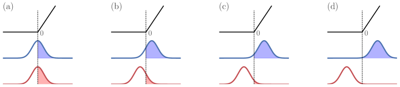
Figure 1: Channel-wise collapse induces channel-wise linearity. Each subplot shows $\phi=\operatorname*{ReLU}$ (black activation function) as well as two channel-wise distributions (blue and red distributions) positioned symmetrically around $0$ with $\frac{\mathcal{P}_{c}(\tilde{{\mathbf{y}}}^{l})-\mathcal{P}^{(1)}_{c}(\tilde{{\mathbf{y}}}^{l})}{\mathcal{P}_{c}(\tilde{{\mathbf{y}}}^{l})}=1,\frac{1}{2},\frac{1}{4},\frac{1}{8}$ for (a), (b), (c), (d), respectively. When progressing from (a) to (d), the part of the distribution corresponding to active $\operatorname*{ReLU}$ (shaded region) becomes either overly dominant (blue distribution) or negligible (red distribution). In either case, the channel-wise distribution ends up concentrated on only one side of piece-wise linearity.

Revisiting BN’s preservation of expressivity.

When BN is used, $\mathcal{P}^{(1)}_{c}({\mathbf{y}}^{l})=0$ implies for all $c$ that the terms $\mathcal{P}^{(2)}_{c}({\mathbf{y}}^{l}),\mathcal{P}^{(3)}_{c}({\mathbf{y}}^{l}),\mathcal{P}^{(4)}_{c}({\mathbf{y}}^{l})$ sum to one. Apart from that, BN does not impose any particular constraints on the relative proportions of each term into the sum. This means that the relative proportions of $\mathcal{P}^{(i)}_{c}({\mathbf{y}}^{l})$ and $\mathcal{P}^{(i)}({\mathbf{y}}^{l})$ for $i\in\{2,3,4\}$ are free to evolve as naturally dictated by the task and the optimizer during learning.

This absence of constraints seems sensible. Indeed, imposing constraints on these relative proportions would alter the expressivity, which would not have any obvious justification in general and could even be detrimental in some cases, as we discuss in Section 4.

4 Failure modes with batch-independent normalization

With our theoretical framework in hand, we now turn to showing that the prototypical batch-independent norms are subject to failures modes opposite to BN’s beneficial properties.

In the case of LN, the failure mode does not manifest in an absolute sense but rather as a soft inductive bias, i.e. as a preference or a favoring in the hypothesis space. This soft inductive bias is quantified by Theorem 1 in the context of networks with random model parameters.

Definition 1 (random net).

We define a random net as a neural network having an input ${\mathbf{x}}$ sampled from the dataset $\mathcal{D}$ and implementing Eq. (2), (3), (4) in every layer up to depth $L$, with the components of ${\bm{\omega}}^{l}$,${\bm{\gamma}}^{l}$,${\bm{\beta}}^{l}$ at every layer $l\in\{1,\dots,L\}$ sampled i.i.d. from the fixed distributions $\nu_{{\bm{\omega}}}$,$\nu_{{\bm{\gamma}}}$,$\nu_{{\bm{\beta}}}$ (up to a fan-in’s square root scaling for ${\bm{\omega}}^{l}$).

In such networks, we assume that: (i) none of the inputs in the dataset $\mathcal{D}$ are identically zero; (ii) $\nu_{{\bm{\omega}}}$, $\nu_{{\bm{\beta}}}$, $\nu_{{\bm{\gamma}}}$ have well-defined moments, with strictly positive associated root mean squares $\omega,\gamma,\beta>0$; (iii) $\nu_{{\bm{\omega}}}$, $\nu_{{\bm{\beta}}}$ are symmetric around zero.

Theorem 1 (layer-normalized networks collapse (informal)).

[D.3] Fix a layer $l\in\{1,\dots,L\}$ and $\nu_{{\bm{\omega}}}$, $\nu_{{\bm{\beta}}}$, $\nu_{{\bm{\gamma}}}$, $\mathcal{D}$ in Definition 1. Further suppose $\operatorname{Norm}=\operatorname{LN}$ and suppose that the convolution of Eq. (2) uses periodic boundary conditions.

Then for random nets of Definition 1, it holds when widths are large enough that

$$\mathcal{P}({\mathbf{y}}^{l})-\mathcal{P}^{(1)}({\mathbf{y}}^{l}) \lesssim\rho^{l-1}, \quad\mathcal{P}({\mathbf{y}}^{l}) \simeq 1,$$ (6)

where $\rho\equiv\gamma^{2}/(\gamma^{2}+\beta^{2})<1$, and $\lesssim$ and $\simeq$ denote inequality and equality up to arbitrarily small constants with probability arbitrarily close to 1 when $\min_{1\leq k\leq l}C_{k}$ is large enough.

Discussion on LN’s failure mode.

Theorem 1 implies that, with high probability, ${\mathbf{y}}^{l}$ is subject to channel-wise collapse in deep layers ($l\gg 1$) with $\mathcal{P}({\mathbf{y}}^{l})-\mathcal{P}^{(1)}({\mathbf{y}}^{l})\ll\mathcal{P}({\mathbf{y}}^{l})$. This means that $\tilde{{\mathbf{y}}}^{l}$ (that is only one affine transformation away from ${\mathbf{y}}^{l}$) is likely to have its channel-wise distributions collapsed with $\mathcal{P}_{c}(\tilde{{\mathbf{y}}}^{l})-\mathcal{P}^{(1)}_{c}(\tilde{{\mathbf{y}}}^{l})\ll\mathcal{P}_{c}(\tilde{{\mathbf{y}}}^{l})$ for most $c$. The nonlinearity $\phi$ acting on $\tilde{{\mathbf{y}}}^{l}$ is then likely to be close to linear with respect to $\tilde{{\mathbf{y}}}^{l}$’s channel-wise distributions [C.2]. Being close to channel-wise linear in deep layers, layer-normalized networks are unable to effectively use their whole depth.

Since the inequality $\lesssim$ can be replaced by an equality $\simeq$ in the case $\phi=\operatorname*{identity}$ of Theorem 1 [D.4], the aggravation at each layer $l$ of the upper bound of Eq. (6) does not stem from the activation function itself but rather by the preceding affine transformation. The phenomenon of channel-wise collapse — also known under the terms of domain collapse [39] or elimination singularity [18] — is therefore not only induced by a mean-shifting activation function such as $\phi=\operatorname*{ReLU}$ [62, 20], but also by the injection of non-centeredness through the application of the channel-wise shift parameter ${\bm{\beta}}^{l}$ at each layer $l$. The fact that the general case of positive homogeneous $\phi$ is upper bounded by the case $\phi=\operatorname*{identity}$ in Eq. (6) still means that the choice $\phi=\operatorname*{ReLU}$ can only be an aggravating factor.

Crucially, in the context of random nets of large widths, LN’s operation at each layer $l$ does not compensate this mean shift. This comes from the fact that LN’s mean and variance statistics can be approximated by zero and a constant value independent of ${\mathbf{x}}$, respectively. This means that LN’s operation can be approximated by a layer-wise constant scaling independent of ${\mathbf{x}}$.

The predominance of LN’s failure mode in the hypothesis space — implied by its predominance in random nets — is expected to have at least two negative effects on the actual learning and final performance: (i) being expected along the training trajectory and being associated with reduced effective capacity, the failure mode is expected to cause degraded performance on the training loss; (ii) even if avoided to some extent along the training trajectory, the failure mode is still expected in the vicinity of this training trajectory, implying an ill-conditioning of the loss landscape [62, 64] and a prohibition of large learning rates that could have led otherwise to generalization benefits [65].

After detailing LN’s failure mode, we now detail IN’s failure mode.

Theorem 2 (instance-normalized networks lack variability in instance statistics).

[E] Fix a layer $l\in\{1,\dots,L\}$ and lift any assumptions on $\phi$. Further suppose $\operatorname{Norm}=\operatorname{IN}$, with Eq. (3) having nonzero denominator at layer $l$ for all inputs and channels.

Then it holds that

• ${\mathbf{y}}^{l}$ is normalized in each channel $c$ with

  $$\mathcal{P}^{(1)}_{c}({\mathbf{y}}^{l}) =0, \quad\mathcal{P}_{c}({\mathbf{y}}^{l}) =1;$$

• ${\mathbf{y}}^{l}$ lacks variability in instance statistics in each channel $c$ with

  $$\mathcal{P}^{(2)}_{c}({\mathbf{y}}^{l}) =0, \quad\mathcal{P}^{(3)}_{c}({\mathbf{y}}^{l}) =1, \quad\mathcal{P}^{(4)}_{c}({\mathbf{y}}^{l}) =0.$$

Discussion on IN’s failure mode.

We see in Theorem 2 that ${\mathbf{y}}^{l}$’s power decomposition with IN is constrained to be such that $\mathcal{P}^{(1)}({\mathbf{y}}^{l}),\mathcal{P}^{(2)}({\mathbf{y}}^{l}),\mathcal{P}^{(4)}({\mathbf{y}}^{l})=0$ and $\mathcal{P}^{(3)}({\mathbf{y}}^{l})=1$. While the constraints on $\mathcal{P}^{(1)}(\tilde{{\mathbf{y}}}^{l})$, $\mathcal{P}^{(3)}(\tilde{{\mathbf{y}}}^{l})$ are removed by the affine transformation between ${\mathbf{y}}^{l}$ and $\tilde{{\mathbf{y}}}^{l}$, the constraints on $\mathcal{P}^{(2)}(\tilde{{\mathbf{y}}}^{l})$, $\mathcal{P}^{(4)}(\tilde{{\mathbf{y}}}^{l})$, on the other hand, remain even after the affine transformation. These constraints on $\mathcal{P}^{(2)}(\tilde{{\mathbf{y}}}^{l})$, $\mathcal{P}^{(4)}(\tilde{{\mathbf{y}}}^{l})$ translate into $2C_{l}$ fixed constraints in activation space that apply to each $\tilde{{\mathbf{y}}}^{l}\in\mathbb{R}^{H\times W\times C_{l}}$ associated with each choice of input ${\mathbf{x}}$ in the dataset $\mathcal{D}$ [53].

Such constraints on $\tilde{{\mathbf{y}}}^{l}$ are symptomatic of an alteration of expressivity. They notably entail that some network mappings that can be expressed without normalization cannot be expressed with IN. One such example is the identity mapping [C.3]. Another such example is a network mapping that would provide in channel $c$ through $\tilde{{\mathbf{y}}}^{l}_{\alpha,c}$, just before the nonlinearity, a detector of a given concept at position $\alpha$ in the input ${\mathbf{x}}$. With IN, the lack of variability in instance statistics implies that the mean $\mu_{{\mathbf{x}},c}(\tilde{{\mathbf{y}}}^{l})$ and standard deviation $\sigma_{{\mathbf{x}},c}(\tilde{{\mathbf{y}}}^{l})$ of the feature map in channel $c$ are necessarily constant for all ${\mathbf{x}}$, equal to ${\bm{\beta}}_{c}$ and ${\bm{\gamma}}_{c}$, respectively. This does not allow to express for some inputs ${\mathbf{x}}$ the presence of the concept at some position $\alpha$: $\mu_{{\mathbf{x}},c}(\tilde{{\mathbf{y}}}^{l})>0$, $\sigma_{{\mathbf{x}},c}(\tilde{{\mathbf{y}}}^{l})>0$; and for other inputs ${\mathbf{x}}$ the absence of the concept: $\mu_{{\mathbf{x}},c}(\tilde{{\mathbf{y}}}^{l})=0$, $\sigma_{{\mathbf{x}},c}(\tilde{{\mathbf{y}}}^{l})=0$.

This latter example is not just anecdotal. Indeed, it is accepted that networks trained on high-level conceptual tasks have their initial layers related to low-level features and their deep layers related to high-level concepts [66, 67]. This view explains the success of IN on the low-level task of style transfer with fixed style input, IN being then incorporated inside a generator network that only acts on the low-level features of the content input [10, 68, 69, 70]. On high-level conceptual tasks, on the other hand, this view hints at a harmful tension between IN’s constraints and the requirement of instance variability to express high-level concepts in deep layers. In short, with IN not only is the expressivity altered, but the alteration of expressivity results in the exclusion of useful network mappings.

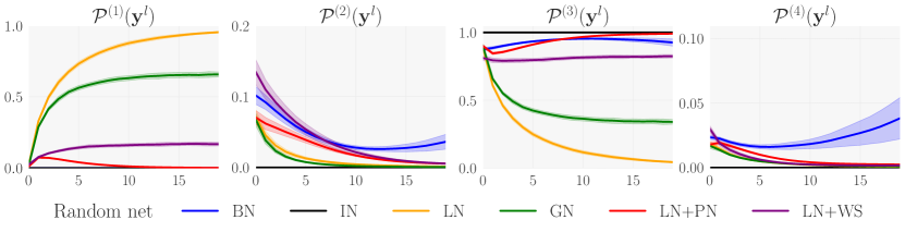
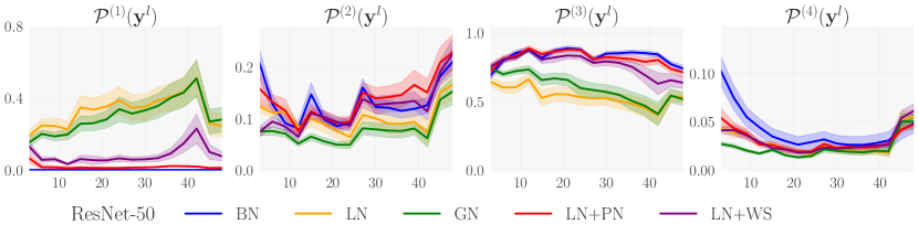
Figure 2: “Power plots”. The power decomposition of ${\mathbf{y}}^{l}$ is shown as a function of the depth $l$ for BN and different batch-independent norms: IN, LN, GN, LN+PN, LN+WS. Top row: Random net of Definition 1 with $\phi=\operatorname*{ReLU}$, widths $C_{l}=1024$, kernel sizes $K_{l}=3$, convolutions using periodic boundary conditions and components of ${\bm{\beta}}^{l}$, ${\bm{\gamma}}^{l}$ sampled i.i.d. from $\mathcal{N}(0,0.2^{2})$ and $\mathcal{N}(1,0.2^{2})$, respectively. Bottom row: ResNet-50 (v2) throughout 100 epochs of training on ImageNet (IN is not shown in this row due to numerical stability issues). Further experimental details are reported in Appendix A.2.

Failure modes with GN.

Group Normalization is a middle ground between the two extremes of LN ($G=1$ group) and IN ($G=C_{l}$ groups at layer $l$). Networks with GN are consequently affected by both failure modes of Theorem 1 and Theorem 2, but to a lesser extent than networks with LN for the failure mode of Theorem 1 and IN for the failure mode of Theorem 2. On the one hand, since GN becomes equivalent to a constant scaling when group sizes become large, networks with GN are likely to be subject to channel-wise collapse. On the other hand, since GN can be seen as removing a fraction — with an inverse dependence on the group size — of $\smash{\mathcal{P}^{(2)}({\mathbf{y}}^{l})}$, $\smash{\mathcal{P}^{(4)}({\mathbf{y}}^{l})}$ in between each layer, networks with GN are likely to lack variability in instance statistics.

The balance struck by GN between the two failure modes of LN and IN could still be beneficial, which would explain GN’s superior performance in practice. It makes sense intuitively that being weakly subject to two failure modes is preferable over being strongly subject to one failure mode.

Experimental validation.

The power plots of Figure 2 show the power decomposition of ${\mathbf{y}}^{l}$ as a function of the depth $l$ in both a random net of Definition 1 and ResNet-50 (v2) [71] trained on ImageNet. Looking at the cases of BN and IN, LN, GN in these power plots, we confirm that: (i) unlike networks with BN and IN, networks with LN, and to a lesser extent GN, are subject to channel-wise collapse as depth increases (see Appendix A.2.1 for a precise verification of Theorem 1); (ii) networks with IN, and to a lesser extent GN, lack variability in instance statistics.

5 Proxy Normalization

With the goal of remedying the failure modes of Section 4, we now introduce our novel technique Proxy Normalization (PN) that is at the core of our batch-independent normalization approach.

PN is incorporated into the neural network by replacing the activation step of Eq. (4) by the following proxy-normalized activation step (cf Figure 3 and the practical implementation of Appendix B):

$$\tilde{{\mathbf{z}}}^{l} =\operatorname{PN-Act}({\mathbf{y}}^{l}), \quad\forall\alpha,c:\quad\operatorname{PN-Act}({\mathbf{y}}^{l})_{\alpha,c}=\frac{\phi\big{(}{\bm{\gamma}}^{l}_{c}{\mathbf{y}}^{l}_{\alpha,c}+{\bm{\beta}}^{l}_{c}\big{)}-\mathbb{E}_{Y^{l}_{c}}\big{[}\phi\big{(}{\bm{\gamma}}^{l}_{c}Y^{l}_{c}+{\bm{\beta}}^{l}_{c})\big{]}}{\sqrt{\mathrm{Var}_{Y^{l}_{c}}\big{[}\phi\big{(}{\bm{\gamma}}^{l}_{c}Y^{l}_{c}+{\bm{\beta}}^{l}_{c})\big{]}+\epsilon}},$$ (7)

where $\epsilon\geq 0$ is a numerical stability constant and $Y^{l}_{c}$ is a Gaussian proxy variable of mean $\tilde{{\bm{\beta}}}^{l}_{c}$ and variance $(1+\tilde{{\bm{\gamma}}}^{l}_{c})^{2}$ depending on the additional parameters $\tilde{{\bm{\beta}}}^{l},\tilde{{\bm{\gamma}}}^{l}\in\mathbb{R}^{C_{l}}$ of PN. Unless otherwise stated, we let $\tilde{{\bm{\beta}}}^{l}$, $\tilde{{\bm{\gamma}}}^{l}$ be nonzero but still subject to weight decay and thus close to zero. We show in Appendix A.3.3 that it is also effective to let $\tilde{{\bm{\beta}}}^{l}$, $\tilde{{\bm{\gamma}}}^{l}$ be strictly zero and $Y^{l}_{c}\sim\mathcal{N}(0,1)$.

If we assume (as hinted by Section 4) that only the affine transformation and the activation function $\phi$ (i.e. the activation step) play a role in the aggravation at each layer $l$ of channel-wise collapse and channel imbalance, then PN provides the following guarantee of channel-wise normalization.

Theorem 3 (guarantee of channel-wise normalization in proxy-normalized networks (informal)).

[F] Fix a layer $l\in\{1,\dots,L\}$ and lift any assumptions on $\phi$ and ${\mathbf{x}}$’s distribution. Further suppose that the neural network implements Eq. (2), (3), (7) at every layer up to depth $L$, with $\epsilon=0$ and Eq. (3), (7) having nonzero denominators for all layers, inputs and channels.

Then both ${\mathbf{y}}^{l}$ and $\tilde{{\mathbf{z}}}^{l}$ at layer $l$ are channel-wise normalized if the following conditions hold:

1. $\tilde{{\mathbf{z}}}^{l-1}$ at layer $l-1$ is channel-wise normalized;

2. The convolution and normalization steps at layer $l$ do not cause any aggravation of channel-wise collapse and channel imbalance;

3. ${\mathbf{y}}^{l}$ at layer $l$ is channel-wise Gaussian and PN’s additional parameters $\tilde{{\bm{\beta}}}^{l}$, $\tilde{{\bm{\gamma}}}^{l}$ are zero.

Our batch-independent approach: LN+PN or GN+PN.

At this point, we crucially note that PN: (i) is batch-independent; (ii) does not cause any alteration of expressivity. This leads us to adopt a batch-independent normalization approach that uses either LN or GN (with few groups) in the normalization step and that replaces the activation step by the proxy-normalized activation step (+PN). With such a choice of normalization step, we guarantee three of the benefits detailed in Table 1: scale invariance, control of activation scale and preservation of expressivity. With the proxy-normalized activation step, we finally guarantee the fourth benefit of avoidance of collapse without compromising any of the benefits provided by the normalization step.

Experimental validation.

We confirm in Figure 2 that BN’s behavior is emulated in a fully batch-independent manner with our approach, LN+PN or GN+PN. Indeed, the power plots of networks with LN+PN resemble the power plots of networks with BN. As desired, PN remedies LN’s failure mode without incurring IN’s failure mode.

Figure 3: Plugging PN. PN is plugged into the activation step $\operatorname{Act}$ to yield the proxy-normalized activation step $\operatorname{PN-Act}$.

Approach strength 1: Normalizing beyond initialization.

Our batch-independent approach maintains channel-wise normalization throughout training (cf Figure 2). In contrast, many alternative approaches, either explicitly or implicitly, focus on initialization [21, 24, 17, 18, 49, 20, 72]. Centered Weight Normalization [17], WS [18, 20, 72] or PreLayerNorm [49] notably rely on the implicit assumption that different channels have the same channel-wise means after the activation function $\phi$. While valid in networks at initialization with ${\bm{\beta}}^{l}=0$ and ${\bm{\gamma}}^{l}=1$ (cf Appendix A.2.2), this assumption becomes less valid as the affine transformation starts deviating from the identity. We see in Figure 2 that networks with LN+WS are indeed less effective in maintaining channel-wise normalization, both in networks with random ${\bm{\beta}}^{l}$, ${\bm{\gamma}}^{l}$ (top row) and in networks considered throughout training (bottom row). Such a coarser channel-wise normalization might in turn lead to a less effective use of model capacity and a degradation of the conditioning of the loss landscape [62, 64].

Approach strength 2: Wide applicability.

Our batch-independent approach matches BN with consistency across choices of model architectures, model sizes and activation functions (cf Section 6). Its only restriction, namely that activation steps should be immediately preceded by normalization steps for ${\mathbf{y}}^{l}$ and its associated proxy $Y^{l}$ to be at the same scale, has easy workarounds. Applicability restrictions might be more serious with alternative approaches: (i) alternative approaches involving a normalization in weight space [16, 17, 18, 19, 20] might be ill-suited to architectures with less dense kernels such as EfficientNets [20]; (ii) approaches involving the tracking of activation statistics [21, 22, 23] might be nontrivial to apply to residual networks [73, 74]; (iii) approaches involving a change of activation function [24, 5, 15] might precisely restrict the choice of activation function.

Approach strength 3: Ease of implementation.

Our approach is straightforward to implement when starting from a batch-normalized network. It simply requires: (i) replacing all BN steps with LN or GN steps, and (ii) replacing all activation steps with proxy-normalized activation steps. The proxy-normalized activation steps themselves are easily implemented (cf Appendix B).

6 Results

We finally assess the practical performance of our batch-independent normalization approach. While we focus on ImageNet [75] in the main text of this paper, we report in Appendix A some additional results on CIFAR [76]. In Appendix A, we also provide all the details on our experimental setup.

Choices of regularization and batch size.

As mentioned in Section 2, we perform all our experiments with different degrees of regularization to disentangle normalization’s effects from regularization’s effects. We detail all our choices of regularization in Appendices A.1 and A.3.4.

In terms of batch size, we set: (i) the global batch size in between weight updates to the same value independently of the choice of norm; (ii) the normalization batch size to a near-optimal value with BN. These choices enable us to be conservative when concluding on a potential advantage of our approach over BN at small batch size. Indeed, while the performance of batch-independent approaches would remain the same or slightly improve at small batch size [77, 65], the performance of BN would eventually degrade due to a regularization that eventually becomes excessive [2, 3, 4, 5, 6, 7].

Effect of adding PN.

We start as a first experiment by analyzing the effect of adding PN on top of various norms in ResNet-50 (RN50). As visible in Table 2, PN is mostly beneficial when added on top of LN or GN with a small number of groups $G$. The consequence is that the optimal $G$ shifts to lower values in GN+PN compared to GN. This confirms the view that PN’s benefit lies in addressing LN’s failure mode.

It is also visible in Table 2 that PN does not provide noticeable benefits to BN. This confirms again the view that PN’s benefit lies in addressing the problem — not present with BN — of channel-wise collapse. Importantly, since PN does not entail effects other than normalization that could artificially boost the performance, GN+PN can be compared in a fair way to BN when assessing the effectiveness of normalization.

Table 2: Effect of adding PN. ResNet-50 is trained on ImageNet with BN and LN, GN, GN+WS with $G$ groups, either without or with PN added on top (plain vs. PN). Results are formatted as X / Y with X, Y the validation accuracies (%) without and with extra regularization, respectively.

		RN50
	$G$	plain	+PN
BN		76.3 / 75.8	76.2 / 76.0
LN	1	74.5 / 74.6	75.9 / 76.5
GN	8	75.4 / 75.4	76.3 / 76.7
GN	32	75.4 / 75.3	75.8 / 76.1
GN+WS	8	76.6 / 76.7	76.8 / 77.1

This is unlike WS which has been shown to improve BN’s performance [18]. In our results of Table 2, the high performance of GN+WS without extra regularization and the fact that PN still provides benefits to GN+WS suggests that: (i) on top of its normalization benefits, WS induces a form of regularization; (ii) GN+WS is still not fully optimal in terms of normalization.

GN+PN vs. BN.

Next, we turn to comparing the performance of our batch-independent approach, GN+PN, to that of BN across a broad range of models trained on ImageNet. As visible in Figure 4 and Tables 3, 4, GN+PN outperforms BN in ResNet-50 (RN50) and ResNet-101 (RN101) [71], matches BN in ResNeXt-50 (RNX50) and ResNeXt-101 (RNX101) [78], and matches BN in EfficientNet-B0 (EN-B0) and EfficientNet-B2 (EN-B2), both in the original variant with depthwise convolutions and expansion ratio of 6 [52] and in an approximately parameter-preserving variant (cf Appendix A.1) with group convolutions of group size 16 and expansion ratio of 4 [79]. In short, our batch-independent normalization approach, GN+PN, matches BN not only in behavior but also in performance.

With regard to matching BN’s performance with alternative norms, various positive results have been reported in ResNets and ResNeXts [8, 7, 12, 13, 15, 20, 36] but only a limited number in EfficientNets [15]. In EfficientNets, we are notably not aware of any other work showing that BN’s performance can be matched with a batch-independent approach. As a confirmation, we assess the performance of various existing batch-independent approaches: GN [3], GN+WS [18], Evo-S0 [15], FRN+TLU [80, 5]. Unlike GN+PN, none of these approaches is found in Table 4 to match BN with consistency.

Normalization and regularization.

Our results suggest that while an efficient normalization is not sufficient in itself to achieve good performance on ImageNet, it is still a necessary condition, together with regularization. In our results, it is always with extra regularization that GN+PN yields the most benefits. Importantly, the fact that GN+PN consistently leads to large improvements in training accuracy (cf Appendix A.3.2) suggests that additional benefits would be obtained on larger datasets without the requirement of relying on regularization [81, 72].

Figure 4: BN vs. GN, GN+PN. Validation accuracies (%) of ResNets, ResNeXts and EfficientNets trained on ImageNet with BN and GN, GN+PN, without and with extra regularization. EfficientNets are considered in the variant with group convolutions [79].

Table 3: BN vs. GN, GN+PN. ResNets and ResNeXts are trained on ImageNet with BN and GN, GN+PN. Results are formatted as in Table 2.

	RN50	RN101	RNX50	RNX101
BN	76.3 / 75.8	77.9 / 78.0	77.6 / 77.2	78.7 / 78.9
GN	75.4 / 75.3	77.0 / 77.4	76.2 / 76.6	77.4 / 78.1
GN+PN	76.3 / 76.7	77.6 / 78.6	76.7 / 77.8	77.7 / 79.0

Table 4: BN vs. batch-independent approaches. EfficientNets are trained on ImageNet with BN and various batch-independent approaches. Results are formatted as in Table 2.

	depthwise convs [52]		group convs [79]
	EN-B0	EN-B2	EN-B0	EN-B2
BN	76.9 / 77.2	79.4 / 80.0	76.8 / 76.7	79.5 / 79.7
GN	76.2 / 76.2	78.9 / 79.4	76.2 / 76.2	79.0 / 79.6
GN+PN	76.8 / 77.0	79.3 / 80.0	76.7 / 76.8	79.3 / 80.1
Evo-S0	75.8 / 75.8	78.5 / 78.7	76.2 / 76.5	78.9 / 79.6
GN+WS	74.2 / 74.1	77.8 / 77.8	76.2 / 76.3	79.2 / 79.4
FRN+TLU	75.7 / 75.7	78.4 / 78.8	74.9 / 75.1	78.2 / 78.6

7 Summary and broader impact

We have introduced a novel framework to finely characterize the various neural network properties affected by the choice of normalization. Using this framework, we have shown that while BN’s beneficial properties are not retained when solely using the prototypical batch-independent norms, they are retained when combining some of these norms with the technique hereby introduced of Proxy Normalization. We have demonstrated on an extensive set of experiments that our batch-independent normalization approach consistently matches BN in both behavior and performance.

The main implications of this work could stem from the unlocked possibility to retain BN’s normalization benefits while removing batch dependence. Firstly, our approach could be used to retain BN’s normalization benefits while alleviating the burden of large activation memory stemming from BN’s requirement of sufficiently large batch sizes. This is expected to be important in memory-intensive applications such as object detection or image segmentation, but also when using A.I. accelerators that leverage local memory to provide extra acceleration and energy savings in exchange for tighter memory constraints. Secondly, our approach could be used to retain BN’s normalization benefits while avoiding BN’s regularization when the latter is detrimental. As discussed in Section 6, this is expected to be important in the context — that will likely be prevalent in the future — of large datasets.

Appendix A Experimental details

A.1 Experimental setup

Architectures.

As stated in Section 5, we use v2 instantiations of ResNets and instantiations of ResNeXts having the same reordering of operations inside residual blocks as ResNets v2. Practically, our instantiations of ResNeXts are obtained by starting from ResNets v2 and applying the same changes in bottleneck widths and number of groups in $3\times 3$ convolutions as the changes yielding ResNeXts v1 from ResNets v1, using a cardinality $32$ and a dimension $4$ [78].

As also stated in Section 6, we consider two variants of EfficientNets: (i) the original variant with one depthwise convolution per MBConv block and with expansion ratio of 6 [52], and (ii) a variant with each depthwise convolution replaced by a group convolution of group size 16 and with expansion ratio of 4 [79]. Compared to the original variant, the variant with group convolutions has roughly the same number of parameters and slightly more floating point operations (FLOPs) (cf Table 5), but it is executed more efficiently on common A.I. accelerators. Interestingly, the fact that GN+WS does not perform well even in this variant (cf Tables 4, 8 and Figure 7) suggests that the problem related to the removal of degrees of freedom by WS goes beyond just depthwise convolutions [20].

Table 5: Number of parameters and number of FLOPs in EfficientNets. Quantities are reported for EfficientNets-B0 (EN-B0) and EfficientNets-B2 (EN-B2) in the variant with depthwise convolutions and expansion ratio of 6 (left) and in the variant with group convolutions of group size 16 and expansion ratio of 4 (right).

	depthwise convs		group convs
	EN-B0	EN-B2	EN-B0	EN-B2
Number of parameters	5.3M	9.1M	5.9M	9.5M
Number of FLOPs	0.4B	1.0B	0.6B	1.5B

PN.

We always set PN’s numerical stability constant to $\epsilon=0.03$, as we found smaller $\epsilon$ can lead to suboptimal performance. We use $200$ samples uniformly sampled in probability in the proxy distribution (cf Appendix B).

In all networks, we disable the scaling part of PN in the proxy-normalized activation step just before the final mean pooling. This is to avoid an alteration of the effective learning rate. An alternative option would be to altogether remove PN before the final mean pooling.

In EfficientNets, we disable PN in squeeze-excite (SE) blocks given that no normalization step precedes each activation step in these blocks. When PN’s additional parameters $\tilde{{\bm{\beta}}}^{l}$, $\tilde{{\bm{\gamma}}}^{l}$ are included, we replace the final affine transformation of each MBConv block by a single channel-wise scaling (i.e. we only keep the scaling parameter in the transformation). When PN’s additional parameters $\tilde{{\bm{\beta}}}^{l}$, $\tilde{{\bm{\gamma}}}^{l}$ are omitted, on the other hand, we leave this final affine transformation as it is.

WS.

We set the numerical stability constant of WS to 0.

In all networks, we disable WS in fully-connected layers and in SE blocks. In ResNets and ResNeXts, we add an extra scale parameter after the final convolution of each residual block when using WS.

Evo-S0.

In EfficientNets, the final norm and affine transformation in each MBConv block are replaced by a single affine transformation when using Evo-S0.

Initialization.

We initialize the affine transformation’s parameters as ${\bm{\beta}}^{l}=0$, ${\bm{\gamma}}^{l}=1$, and PN’s additional parameters as $\tilde{{\bm{\beta}}}^{l}=0$, $\tilde{{\bm{\gamma}}}^{l}=0$ when these additional parameters are included. We initialize weights ${\bm{\omega}}^{l}$ by sampling from truncated normal distributions with an inverse square root scaling with respect to fan-in (expect for some kernels in EfficientNets where the scaling is with respect to fan-out).

ResNets and ResNeXts trained on ImageNet.

We train for 100 epochs with SGD with a momentum of $0.9$ and a batch size of 256. We start with a learning rate of 0.1 after a linear warmup over the first 5 epochs [77], and we decrease this learning rate four times at the epochs 30, 60, 80 and 90, each time by a factor $10$. We apply weight decay with a strength of $10^{-4}$ to all parameters including the additional parameters $\tilde{{\bm{\beta}}}^{l}$, $\tilde{{\bm{\gamma}}}^{l}$ of PN and the channel-wise scale and shift parameters ${\bm{\beta}}^{l}$, ${\bm{\gamma}}^{l}$ (this is sensible as $\phi=\operatorname*{ReLU}$ is positive homogeneous).

We set the norm’s numerical stability constant to $10^{-6}$ and, unless otherwise specified, we set the number of groups to $G=8$ when using GN+PN and to $G=32$ when using GN without PN. When using BN, we compute BN’s statistics over 32 inputs ${\mathbf{x}}$ and we compute moving average statistics by exponentially weighted average with decay factor $0.97$.

For the pre-processing, we follow [71]. When using extra regularization, we use label smoothing with factor $0.1$ [82], dropout with rate $0.1$ [83] and stochastic depth with rate $0.05$ [84]. As the only exception, when changing the choice of the extra regularization in Appendix A.3.4, we use Mixup with strength $0.1$ [85] in all networks, and in ResNet-101 and ResNeXt-101, we additionally use a variant of CutMix [86] that samples $U_{0}\sim\operatorname{Uniform}(0,1)$ and $U_{1}\sim\operatorname{Uniform}(e^{-4},1)$ and sets the combination ratio as $\lambda=1$ if $U_{0}\leq 0.435$ and $\lambda=1+\frac{1}{4}\log(U_{1})$ otherwise.

While we use float-16 to store and process intermediate activations (except in normalization steps and PN’s statistics computation), model parameters are still stored and updated in float-32. Each time we provide a result, the mean and standard deviation are computed over 3 independent runs, at the final epoch of each run. As the only exception, the mean and $1\sigma$ intervals in the power plots of Figures 2, 6 are computed by pooling together either all 100 epochs in 5 independent runs (Figure 2) or the initialization state in 5 independent runs (Figure 6).

EfficientNets with batch-independent norms trained on ImageNet.

Our experimental setup closely follows [52]. We train for 350 epochs with RMSProp with a batch size of 768. We start with a learning rate of $768\times 2^{-14}$ (i.e. using a linear scaling [65]) after a linear warmup over the first 5 epochs [77], and we decay the learning rate exponentially by a factor 0.97 every 2.4 epochs. In RMSProp, we use a momentum of 0.9, a decay of $1.0-(768\times 2^{-14})$ and a numerical stability constant of $10^{-3}$. We apply weight decay with a strength of $10^{-5}$ on the convolutional weights and the additional parameters $\tilde{{\bm{\beta}}}^{l}$, $\tilde{{\bm{\gamma}}}^{l}$ of PN, but not on the other channel-wise parameters (this is sensible as $\phi=\operatorname*{Swish}$ is not positive homogeneous).

We set the norm’s numerical stability constant to $10^{-3}$ and we set the number of groups to $G=4$ when using GN or Evo-S0.

For the baseline pre-processing, we follow [52]. In terms of regularization, we always use label smoothing with factor $0.1$ [82], dropout with rate $0.2$ [83] and stochastic depth with rate starting at $0.2$ in the first MBConv block and decaying to zero linearly with the depth of the MBConv block [84]. When using extra regularization, we use Mixup with strength $0.1$ [85] in all networks, and in EfficientNets-B2, we additionally use a variant of CutMix [86] that samples $U_{0}\sim\operatorname{Uniform}(0,1)$ and $U_{1}\sim\operatorname{Uniform}(e^{-4},1)$ and sets the combination ratio as $\lambda=1$ if $U_{0}\leq 0.435$ and $\lambda=1+\frac{1}{4}\log(U_{1})$ otherwise.

While we use float-16 to store and process intermediate activations (except in normalization steps and PN’s statistics computation), model parameters are still stored and updated in float-32. Each time we provide a result, the mean and standard deviation are computed over 3 independent runs. For each run, performance is evaluated at the final epoch, with model parameters obtained by exponentially weighted average with decay factor $0.97$ over checkpoints from previous epochs.

EfficientNets with BN trained on ImageNet.

For these experiments, we run the public EfficientNet repository with the settings recommended in the repository. When considering the variant with group convolutions, our only modifications consist in (i) replacing depthwise convolutions with group convolutions of group size 16, and (ii) changing the expansion ratio from 6 to 4.

In addition to BN’s inherent regularization, these runs always incorporate label smoothing [82], dropout [83] and stochastic depth [84]. The runs with extra regularization additionally incorporate AutoAugment [87].

Each time we provide a result, the mean and standard deviation are computed over 3 independent runs.

ResNets trained on CIFAR-10 and CIFAR-100 (cf Appendix A.4).

We train for 160 epochs with SGD with a momentum of $0.9$ and a batch size of 128. We start with a learning rate of 0.1 after a linear warmup over the first 5 epochs [77], and we decrease this learning rate two times at the epochs 80 and 120, each time by a factor $10$. We apply weight decay with a strength of $10^{-4}$ to all parameters including the additional parameters $\tilde{{\bm{\beta}}}^{l}$, $\tilde{{\bm{\gamma}}}^{l}$ of PN and the channel-wise scale and shift parameters ${\bm{\beta}}^{l}$, ${\bm{\gamma}}^{l}$ (this is sensible as $\phi=\operatorname*{ReLU}$ is positive homogeneous).

We set the norm’s numerical stability constant to $10^{-6}$ and we set the number of groups to $G=4$ when using GN. When using BN, we compute BN’s statistics over 128 inputs ${\mathbf{x}}$ and we compute moving average statistics by exponentially weighted average with decay factor $0.97$.

For the pre-processing, we follow [71]. When using extra regularization, we use label smoothing with factor $0.1$ [82], dropout with rate $0.25$ [83] and stochastic depth with rate $0.1$ [84].

We use float-16 to store and process intermediate activations (except in normalization steps and PN’s statistics computation) and to store and update model parameters. Each time we provide a result, the mean and standard deviation are computed over 10 independent runs, at the final epoch of each run.

Random nets.

We consider random nets following Definition 1. For the cases of BN, IN, LN, GN, random nets implement Eq. (2), (3), (4) at every layer $l$. For the case of LN+PN, we replace the activation step of Eq. (4) by the proxy-normalized activation step of Eq. (7). For the case of LN+WS, we add a step of kernel standardization before the convolution of Eq. (2). In all cases, convolutions use periodic boundary conditions to remain consistent with the assumptions of Theorem 1.

We set the activation function to $\phi=\operatorname*{ReLU}$, widths to $C_{l}=1024$, kernel sizes to $K_{l}=3$.

We sample the components of the affine transformation’s parameters ${\bm{\beta}}^{l}$, ${\bm{\gamma}}^{l}$ i.i.d. from $\nu_{{\bm{\beta}}}=\mathcal{N}(0,0.2^{2})$ and $\nu_{{\bm{\gamma}}}=\mathcal{N}(1,0.2^{2})$, respectively. This yields $\beta^{2}=0.2^{2}$, $\gamma^{2}=1^{2}+0.2^{2}$ and $\rho=\frac{1^{2}+0.2^{2}}{1^{2}+0.2^{2}+0.2^{2}}~{}\approx~{}0.963$ in Definition 1. We sample the components of weight parameters ${\bm{\omega}}^{l}$ i.i.d. from truncated normal distributions with $\frac{1}{\sqrt{C_{l}}}$ scaling. We set PN’s additional parameters $\tilde{{\bm{\beta}}}^{l}$, $\tilde{{\bm{\gamma}}}^{l}$ to 0.

We set the norm’s numerical stability constant to $10^{-6}$ and we set the number of groups to $G=128$ when using GN to roughly preserve group sizes compared to ResNet-50. We use a batch size of 128 and we compute BN’s statistics over all 128 inputs ${\mathbf{x}}$ in the mini-batch when using BN.

We use CIFAR-10 as the dataset $\mathcal{D}$ and we follow [71] for the pre-processing. To alleviate the memory burden, we add a downsampling by setting the stride to $2$ in the first convolution of the network.

We use float-32 to store and process intermediate activations. Each time we provide a result, the mean and $1\sigma$ intervals are computed over 50 independent realizations.

A.I. accelerators.

We run all our experiments with batch-independent norms on Graphcore’s IPUs.

A.2 Additional details on power plots

A.2.1 Power plots in random nets

Additional experimental details.

We obtain the power plots in random nets using the experimental setup described in Appendix A.1 for random nets. We compute the terms $\mathcal{P}^{(1)}({\mathbf{y}}^{l})$, $\mathcal{P}^{(2)}({\mathbf{y}}^{l})$, $\mathcal{P}^{(3)}({\mathbf{y}}^{l})$, $\mathcal{P}^{(4)}({\mathbf{y}}^{l})$ (as well as the additional terms from Figure 5) for each layer $l$ using the 128 randomly sampled inputs ${\mathbf{x}}$ in the mini-batch as a proxy for the full dataset $\mathcal{D}$.

While we set the total depth to $L=200$, we show only the first $20$ layers in Figure 2 to facilitate a side-by-side comparison with ResNet-50. Indeed, while the effective depth is smaller than the computational depth in ResNet-50 (cf Appendix A.2.2), the two notions of depth coincide in random nets.

Verification of Theorem 1.

The case of random nets with LN enables us to precisely verify Theorem 1. We provide this verification in the left and center subplots of Figure 5.

In the left subplot of Figure 5, we show $\mathcal{P}({\mathbf{y}}^{l})-\mathcal{P}^{(1)}({\mathbf{y}}^{l})$ (mean and $1\sigma$ interval) and the upper bound $\rho^{l-1}=\Big{(}\frac{1^{2}+0.2^{2}}{1^{2}+0.2^{2}+0.2^{2}}\Big{)}^{l-1}$ from Theorem 1 for depths $l$ up to $L=200$. We confirm that $\mathcal{P}({\mathbf{y}}^{l})-\mathcal{P}^{(1)}({\mathbf{y}}^{l})$ is upper bounded with high probability by $\rho^{l-1}$ as predicted by Theorem 1. The rate of decay of $\mathcal{P}({\mathbf{y}}^{l})-\mathcal{P}^{(1)}({\mathbf{y}}^{l})$ is initially above the prediction of Theorem 1 due to the aggravating effect of $\phi=\operatorname*{ReLU}$. In very deep layers ($l\gg 1$), this rate of decay ends up very slightly below the prediction of Theorem 1 due to the facts that: (i) $\phi$ becomes effectively close to channel-wise linear; (ii) the channel-wise collapse is slightly mitigated by LN in the case of a finite width $C_{l}=1024$.

In the center subplot of Figure 5, we show $\mathcal{P}({\mathbf{y}}^{l})$ (mean and $1\sigma$ interval) for depths $l$ up to $L=200$. We confirm that $\mathcal{P}({\mathbf{y}}^{l})$ is with high probability very close to one.

Quantification of channel-wise linearity.

To confirm the connection between channel-wise collapse and channel-wise linearity, we finally report the evolution with depth of an additional measure of channel-wise linearity. In the right subplot of Figure 5, we show the measure $\mathcal{P}(\phi(\tilde{{\mathbf{y}}}^{l})-\widetilde{{\mathbf{z}}}^{l})/\mathcal{P}(\phi(\tilde{{\mathbf{y}}}^{l}))$ (mean and $1\sigma$ interval) for depths $l$ up to $L=200$, with $\widetilde{{\mathbf{z}}}^{l}$ the channel-wise linear best-fit of $\phi(\tilde{{\mathbf{y}}}^{l})$ using $\tilde{{\mathbf{y}}}^{l}$, that is defined in Eq. (8), (9). We confirm that deep in random nets, layers are effectively: (i) very close to channel-wise linear with LN; (ii) close to channel-wise linear with GN.

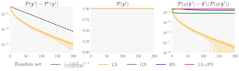
Figure 5: Verification of Theorem 1 and quantification of channel-wise linearity. Results are reported in random nets of Definition 1 for depths $l$ up to $L=200$. Left: $\mathcal{P}({\mathbf{y}}^{l})-\mathcal{P}^{(1)}({\mathbf{y}}^{l})$ (mean and $1\sigma$ interval) and upper bound $\rho^{l-1}$ from Theorem 1. Center: $\mathcal{P}({\mathbf{y}}^{l})$ (mean and $1\sigma$ interval). Right: Additional measure of channel-wise linearity $\mathcal{P}(\phi(\tilde{{\mathbf{y}}}^{l})-\widetilde{{\mathbf{z}}}^{l})/\mathcal{P}(\phi(\tilde{{\mathbf{y}}}^{l}))$ (mean and $1\sigma$ interval), with $\widetilde{{\mathbf{z}}}^{l}$ the channel-wise linear best-fit of $\phi(\tilde{{\mathbf{y}}}^{l})$ using $\tilde{{\mathbf{y}}}^{l}$, that is defined in Eq. (8), (9)

A.2.2 Power plots in ResNet-50

Additional experimental details.

We obtain the power plots in ResNet-50 using the experimental setup described in Appendix A.1 for ResNets on ImageNet. At each epoch, we compute the power terms $\mathcal{P}^{(1)}_{c}({\mathbf{y}}^{l})$, $\mathcal{P}^{(2)}_{c}({\mathbf{y}}^{l})$, $\mathcal{P}^{(3)}_{c}({\mathbf{y}}^{l})$, $\mathcal{P}^{(4)}_{c}({\mathbf{y}}^{l})$ for each layer $l$ and each channel $c$ using the last 256 randomly sampled inputs ${\mathbf{x}}$ as a proxy for the full dataset $\mathcal{D}$.

When looking at each norm separately in ResNets, we noticed artefacts that we attributed to the discrepancy between the computational depth $l$ and the effective depth (that oscillates with $l$). Indeed, the effective depth, defined in terms of the statistical properties of intermediate activations, grows linearly inside each residual block but gets reduced each time a residual path is summed with a skip connection path (since the latter originates from earlier layers). This phenomenon is tightly connected to the property discussed in Section 2 on the control of activation scale in residual networks.

To avoid such an artefact in Figures 2, 6, we report only a single measurement of $\mathcal{P}^{(1)}({\mathbf{y}}^{l})$, $\mathcal{P}^{(2)}({\mathbf{y}}^{l})$, $\mathcal{P}^{(3)}({\mathbf{y}}^{l})$, $\mathcal{P}^{(4)}({\mathbf{y}}^{l})$ per residual block by pooling together all the channels from the three norms inside each residual block. For the same reason, we do not report $\mathcal{P}^{(1)}({\mathbf{y}}^{l})$, $\mathcal{P}^{(2)}({\mathbf{y}}^{l})$, $\mathcal{P}^{(3)}({\mathbf{y}}^{l})$, $\mathcal{P}^{(4)}({\mathbf{y}}^{l})$ for the final norm just before the final mean pooling.

The presence of this artefact confirms the fact that the effective depth evolves more slowly than the computational depth $l$ in residual networks. This explains why ${\mathbf{y}}^{l}$ with LN or GN is not immoderately collapsed even at large $l$ in Figures 2, 6.

Numerical stability issues with IN.

As stated in the caption of Figure 2, we did not succeed at training ResNet-50 v2 with IN. We found that using float-16 to store and process intermediate activations caused divergence in these networks. When replacing float-16 by float-32, even though divergence was avoided, ResNets-50 v2 still did not reach satisfactory performance with IN. We attributed this to a plain incompatibility of IN with v2 instantiations of ResNets, which could stem from the presence of a final block of normalization and activation just before the final mean pooling. Intuitively, if we denote this final block as $L$ and if we subtract away the activation function by supposing $\phi=\operatorname*{identity}$, then $\mu_{{\mathbf{x}},c}({\mathbf{z}}^{L})$ in channel $c$ is constant for all ${\mathbf{x}}$, equal to ${\bm{\beta}}^{L}_{c}$ (cf Section 4). Thus, if we subtract away the activation function, with IN all inputs ${\mathbf{x}}$ end up mapped to the same channel-wise constants after the final mean pooling, i.e. they become indistinguishable.

Power plots at initialization.

Figure 6 reports the same power plots as Figure 2, except with $\mathcal{P}^{(1)}({\mathbf{y}}^{l})$, $\mathcal{P}^{(2)}({\mathbf{y}}^{l})$, $\mathcal{P}^{(3)}({\mathbf{y}}^{l})$, $\mathcal{P}^{(4)}({\mathbf{y}}^{l})$ computed at initialization (mean and $1\sigma$ intervals).

When comparing Figure 6 to Figure 2, it is clearly visible that the channel-wise collapse with LN+WS gets aggravated during training compared to initialization. This confirms the importance of compensating during training the mean shift associated with the affine transformation.

It is also visible that the difference between GN and LN gets narrower during training compared to initialization. This means that despite a similar behavior of $\mathcal{P}^{(1)}({\mathbf{y}}^{l})$ along the training trajectories with GN and LN, differences could still exist in the vicinity of these trajectories, implying a better conditioning of the loss landscape with GN. A similar argument would make us expect a better conditioning of the loss landscape when enforcing ${\mathbf{y}}^{l}$ to be channel-wise normalized via an operation directly embedded in the network mapping [62, 64] as opposed to via an external penalty [88, 49, 89], despite the two approaches potentially leading to the same reduction of $\mathcal{P}^{(1)}({\mathbf{y}}^{l})$.

We believe that the notions of channel-wise collapse and conditioning of the loss landscape [62, 64] enable to quantify more accurately the underlying phenomenons at play than the notion of internal covariate shift [1, 90], despite the former and latter notions being connected.

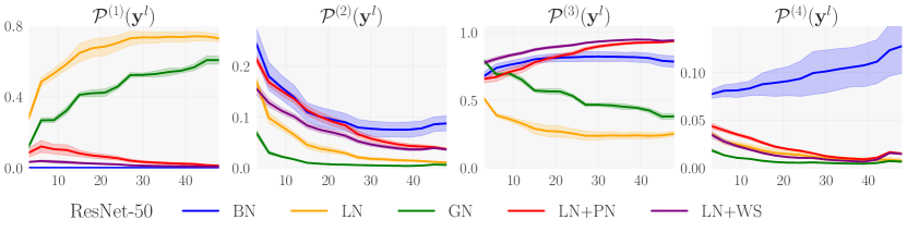
Figure 6: Power plots at initialization. $\mathcal{P}^{(1)}({\mathbf{y}}^{l})$, $\mathcal{P}^{(2)}({\mathbf{y}}^{l})$, $\mathcal{P}^{(3)}({\mathbf{y}}^{l})$, $\mathcal{P}^{(4)}({\mathbf{y}}^{l})$ are shown as a function of the depth $l$ in ResNet-50 at initialization with BN and different batch-independent norms: LN, GN, LN+PN, LN+WS.

A.3 More detailed results on ImageNet

A.3.1 $1\sigma$ intervals

In Tables 6, 7, 8, we complement the results of Tables 2, 3, 4 with $1\sigma$ intervals. In Figure 7, we provide a visualization of the results of Tables 4, 8.

Table 6: Effect of adding PN. ResNet-50 is trained on ImageNet with BN and LN, GN, GN+WS with $G$ groups, either without or with PN added on top (plain vs. PN). Results are formatted as X / Y with X, Y the validation accuracies (mean and $1\sigma$ interval in %) without and with extra regularization, respectively.

		RN50
	$G$	plain	+PN
BN		76.3$\pm$0.1 / 75.8$\pm$0.2	76.2$\pm$0.1 / 76.0$\pm$0.1
LN	1	74.5$\pm$0.0 / 74.6$\pm$0.1	75.9$\pm$0.1 / 76.5$\pm$0.0
GN	8	75.4$\pm$0.1 / 75.4$\pm$0.1	76.3$\pm$0.1 / 76.7$\pm$0.0
GN	32	75.4$\pm$0.1 / 75.3$\pm$0.1	75.8$\pm$0.2 / 76.1$\pm$0.1
GN+WS	8	76.6$\pm$0.0 / 76.7$\pm$0.1	76.8$\pm$0.1 / 77.1$\pm$0.1

Table 7: BN vs. GN, GN+PN. ResNets and ResNeXts are trained on ImageNet with BN and GN, GN+PN. Results are formatted as in Table 6.

	RN50	RN101	RNX50	RNX101
BN	76.3$\pm$0.1 / 75.8$\pm$0.2	77.9$\pm$0.1 / 78.0$\pm$0.1	77.6$\pm$0.1 / 77.2$\pm$0.1	78.7$\pm$0.1 / 78.9$\pm$0.1
GN	75.4$\pm$0.1 / 75.3$\pm$0.1	77.0$\pm$0.1 / 77.4$\pm$0.1	76.2$\pm$0.2 / 76.6$\pm$0.1	77.4$\pm$0.2 / 78.1$\pm$0.1
GN+PN	76.3$\pm$0.1 / 76.7$\pm$0.0	77.6$\pm$0.2 / 78.6$\pm$0.2	76.7$\pm$0.1 / 77.8$\pm$0.2	77.7$\pm$0.2 / 79.0$\pm$0.1

Table 8: BN vs. batch-independent approaches. EfficientNets are trained on ImageNet with BN and various batch-independent approaches: GN, GN+PN, Evo-S0, GN+WS, FRN+TLU. Results are formatted as in Table 6.

	depthwise convs		group convs
	EN-B0	EN-B2	EN-B0	EN-B2
BN	76.9$\pm$0.1 / 77.2$\pm$0.1	79.4$\pm$0.0 / 80.0$\pm$0.0	76.8$\pm$0.1 / 76.7$\pm$0.2	79.5$\pm$0.1 / 79.7$\pm$0.1
GN	76.2$\pm$0.1 / 76.2$\pm$0.1	78.9$\pm$0.1 / 79.4$\pm$0.1	76.2$\pm$0.1 / 76.2$\pm$0.2	79.0$\pm$0.1 / 79.6$\pm$0.1
GN+PN	76.8$\pm$0.0 / 77.0$\pm$0.1	79.3$\pm$0.1 / 80.0$\pm$0.1	76.7$\pm$0.1 / 76.8$\pm$0.1	79.3$\pm$0.1 / 80.1$\pm$0.1
Evo-S0	75.8$\pm$0.1 / 75.8$\pm$0.2	78.5$\pm$0.1 / 78.7$\pm$0.1	76.2$\pm$0.0 / 76.5$\pm$0.1	78.9$\pm$0.0 / 79.6$\pm$0.0
GN+WS	74.2$\pm$0.1 / 74.1$\pm$0.1	77.8$\pm$0.0 / 77.8$\pm$0.1	76.2$\pm$0.1 / 76.3$\pm$0.1	79.2$\pm$0.1 / 79.4$\pm$0.1
FRN+TLU	75.7$\pm$0.1 / 75.7$\pm$0.2	78.4$\pm$0.1 / 78.9$\pm$0.1	74.9$\pm$0.2 / 75.1$\pm$0.1	78.2$\pm$0.1 / 78.6$\pm$0.1

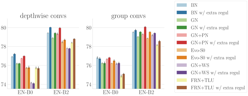
Figure 7: BN vs. batch-independent approaches. Validation accuracies (%) of EfficientNets trained on ImageNet with BN and various batch-independent approaches, without and with extra regularization.

A.3.2 Training accuracies

In Tables 9, 10, 11, we complement the results of Tables 2, 3, 4 with training accuracies.

We stress that these training accuracies are highly dependent on the strength of applied regularization. This leads us to: (i) always separate the training accuracies obtained without and with extra regularization; (ii) report only the training accuracies obtained with batch-independent approaches, given that training accuracies obtained with BN would not be comparable due to BN’s inherent regularization.

As visible in Tables 9, 10, 11, GN+PN outperforms alternative batch-independent approaches in terms of training accuracy on ImageNet. This applies both to training without extra regularization and to training with extra regularization. This suggests that, on larger datasets, GN+PN would outperform these alternative batch-independent approaches in terms of both training and validation accuracies [81, 72].

In Table 11, the fact that with extra regularization EfficientNets-B2 reach lower training accuracies than EfficientNets-B0 is explained by the different level of applied regularization (we add CutMix when training EfficientNets-B2).

Table 9: Training accuracies in ResNet-50. Networks are trained on ImageNet with LN, GN, GN+WS with $G$ groups, either without or with PN added on top (plain vs. +PN). Results are formatted as X with X the training accuracy at the final epoch (mean and $1\sigma$ interval in %). We report separately the results without extra regularization (top) and with extra regularization (bottom).

			RN50
		$G$	plain	+PN
without extra regul	LN	1	75.7$\pm$0.1	79.9$\pm$0.1
	GN	8	77.2$\pm$0.1	80.3$\pm$0.1
	GN	32	77.0$\pm$0.0	79.2$\pm$0.2
	GN+WS	8	80.1$\pm$0.0	80.4$\pm$0.0
with extra regul	LN	1	71.8$\pm$0.1	75.8$\pm$0.0
	GN	8	73.3$\pm$0.1	76.2$\pm$0.1
	GN	32	73.1$\pm$0.1	75.1$\pm$0.1
	GN+WS	8	75.8$\pm$0.0	76.3$\pm$0.0

Table 10: Training accuracies in ResNets and ResNeXts. Networks are trained on ImageNet with GN, GN+PN. Results are formatted as in Table 9.

		RN50	RN101	RNX50	RNX101
without extra regul	GN	77.0$\pm$0.0	79.9$\pm$0.1	79.6$\pm$0.1	81.6$\pm$0.0
	GN+PN	80.3$\pm$0.1	83.5$\pm$0.0	84.1$\pm$0.1	86.2$\pm$0.0
with extra regul	GN	73.1$\pm$0.1	76.5$\pm$0.0	76.0$\pm$0.1	78.6$\pm$0.1
	GN+PN	76.2$\pm$0.1	79.7$\pm$0.1	79.8$\pm$0.0	82.7$\pm$0.0

Table 11: Training accuracies in EfficientNets. Networks are trained on ImageNet with various batch-independent approaches: GN, GN+PN, Evo-S0, GN+WS, FRN+TLU. Results are formatted as in Table 9.

		depthwise convs		group convs
		EN-B0	EN-B2	EN-B0	EN-B2
without extra regul	GN	75.4$\pm$0.0	80.9$\pm$0.1	74.7$\pm$0.0	80.1$\pm$0.1
	GN+PN	77.3$\pm$0.0	82.7$\pm$0.0	75.8$\pm$0.0	81.4$\pm$0.1
	Evo-S0	74.6$\pm$0.2	79.8$\pm$0.2	75.1$\pm$0.0	80.4$\pm$0.1
	GN+WS	71.4$\pm$0.0	77.6$\pm$0.0	74.5$\pm$0.0	80.2$\pm$0.1
	FRN+TLU	75.0$\pm$0.1	80.4$\pm$0.0	72.9$\pm$0.1	78.5$\pm$0.1
with extra regul	GN	71.2$\pm$0.1	66.2$\pm$0.1	70.5$\pm$0.1	65.6$\pm$0.1
	GN+PN	72.8$\pm$0.0	67.8$\pm$0.1	71.5$\pm$0.1	66.7$\pm$0.0
	Evo-S0	70.2$\pm$0.2	64.4$\pm$0.3	70.8$\pm$0.1	65.6$\pm$0.1
	GN+WS	67.3$\pm$0.1	63.4$\pm$0.1	70.4$\pm$0.1	65.4$\pm$0.0
	FRN+TLU	70.4$\pm$0.3	65.1$\pm$0.2	68.8$\pm$0.2	64.0$\pm$0.1

A.3.3 Effect of omitting PN’s additional parameters

In Tables 12, 13 and Figure 8, we report results with PN’s additional parameters $\tilde{{\bm{\beta}}}^{l}$, $\tilde{{\bm{\gamma}}}^{l}$ set to 0. In that case, $\tilde{{\bm{\beta}}}^{l}$, $\tilde{{\bm{\gamma}}}^{l}$ can be equivalently omitted and the proxy variable $Y^{l}$ can be simply considered as a standard Gaussian variable in each channel $c$, i.e. $Y^{l}_{c}\sim\mathcal{N}(0,1)$ (cf our implementation of Appendix B).

As visible in Tables 12, 13 and Figure 8, the omission of PN’s additional parameters $\tilde{{\bm{\beta}}}^{l}$, $\tilde{{\bm{\gamma}}}^{l}$ is indeed harmful. However, the drop of performance that results from omitting $\tilde{{\bm{\beta}}}^{l}$, $\tilde{{\bm{\gamma}}}^{l}$ in GN+PN is very small (in average less than $0.1\%$ in validation accuracy).

Given that the omission of PN’s additional parameters $\tilde{{\bm{\beta}}}^{l}$, $\tilde{{\bm{\gamma}}}^{l}$ leads to slight benefits in terms of computational requirements and simplicity of implementation, this variant of PN with $\tilde{{\bm{\beta}}}^{l}$, $\tilde{{\bm{\gamma}}}^{l}$ omitted might sometimes be a better trade-off.

Table 12: Effect of omitting PN’s additional parameters in ResNets and ResNeXts. Networks are trained on ImageNet with BN and GN, GN+PN with $\tilde{{\bm{\beta}}}^{l}$, $\tilde{{\bm{\gamma}}}^{l}$ included, and GN+PN with $\tilde{{\bm{\beta}}}^{l}$, $\tilde{{\bm{\gamma}}}^{l}$ omitted. Results are formatted as in Table 6.

	RN50	RN101	RNX50	RNX101
BN	76.3$\pm$0.1 / 75.8$\pm$0.2	77.9$\pm$0.1 / 78.0$\pm$0.1	77.6$\pm$0.1 / 77.2$\pm$0.1	78.7$\pm$0.1 / 78.9$\pm$0.1
GN	75.4$\pm$0.1 / 75.3$\pm$0.1	77.0$\pm$0.1 / 77.4$\pm$0.1	76.2$\pm$0.2 / 76.6$\pm$0.1	77.4$\pm$0.2 / 78.1$\pm$0.1
GN+PN with $\tilde{{\bm{\beta}}}^{l}$, $\tilde{{\bm{\gamma}}}^{l}$ included	76.3$\pm$0.1 / 76.7$\pm$0.0	77.6$\pm$0.2 / 78.6$\pm$0.2	76.7$\pm$0.1 / 77.8$\pm$0.2	77.7$\pm$0.2 / 79.0$\pm$0.1
GN+PN with $\tilde{{\bm{\beta}}}^{l}$, $\tilde{{\bm{\gamma}}}^{l}$ omitted	76.3$\pm$0.0 / 76.7$\pm$0.1	77.5$\pm$0.0 / 78.5$\pm$0.1	76.5$\pm$0.1 / 77.6$\pm$0.1	77.5$\pm$0.1 / 79.0$\pm$0.1

Table 13: Effect of omitting PN’s additional parameters in EfficientNets. Networks are trained on ImageNet with BN and GN, GN+PN with $\tilde{{\bm{\beta}}}^{l}$, $\tilde{{\bm{\gamma}}}^{l}$ included, and GN+PN with $\tilde{{\bm{\beta}}}^{l}$, $\tilde{{\bm{\gamma}}}^{l}$ omitted. Results are formatted as in Table 6.

	depthwise convs		group convs
	EN-B0	EN-B2	EN-B0	EN-B2
BN	76.9$\pm$0.1 / 77.2$\pm$0.1	79.4$\pm$0.0 / 80.0$\pm$0.0	76.8$\pm$0.1 / 76.7$\pm$0.2	79.5$\pm$0.1 / 79.7$\pm$0.1
GN	76.2$\pm$0.1 / 76.2$\pm$0.1	78.9$\pm$0.1 / 79.4$\pm$0.1	76.2$\pm$0.1 / 76.2$\pm$0.2	79.0$\pm$0.1 / 79.6$\pm$0.1
GN+PN with $\tilde{{\bm{\beta}}}^{l}$, $\tilde{{\bm{\gamma}}}^{l}$ included	76.8$\pm$0.0 / 77.0$\pm$0.1	79.3$\pm$0.1 / 80.0$\pm$0.1	76.7$\pm$0.1 / 76.8$\pm$0.1	79.3$\pm$0.1 / 80.1$\pm$0.1
GN+PN with $\tilde{{\bm{\beta}}}^{l}$, $\tilde{{\bm{\gamma}}}^{l}$ omitted	76.6$\pm$0.2 / 77.0$\pm$0.1	79.2$\pm$0.0 / 79.9$\pm$0.1	76.7$\pm$0.1 / 76.7$\pm$0.1	79.3$\pm$0.1 / 80.0$\pm$0.2

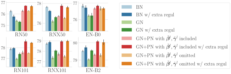
Figure 8: Effect of omitting PN’s additional parameters. Validation accuracies (%) of ResNets, ResNeXts and EfficientNets trained on ImageNet with BN and GN, GN+PN with $\tilde{{\bm{\beta}}}^{l}$, $\tilde{{\bm{\gamma}}}^{l}$ included, and GN+PN with $\tilde{{\bm{\beta}}}^{l}$, $\tilde{{\bm{\gamma}}}^{l}$ omitted, without and with extra regularization. EfficientNets are considered in the variant with group convolutions [79].

A.3.4 Effect of changing the choice of the extra regularization

In Table 14 and Figure 9, we report results in ResNets and ResNeXts with a change in the choice of the extra regularization. When using extra regularization, instead of using label smoothing [82], dropout [83] and stochastic depth [84], we use Mixup [85] in all networks, and in ResNet-101 and ResNeXt-101, we additionally use CutMix [86] (cf Appendix A.1).

We reach similar conclusions with the results of Table 14 and Figure 9 as with the results of Table 7: (i) BN is matched or outperformed by GN+PN, except for a small gap of performance in ResNeXt-50 (this gap of performance might be due to the imperfect abstraction away of regularization); (ii) good performance remains tied to the combination of both an efficient normalization and an efficient regularization.

Table 14: Effect of changing the choice of the extra regularization. ResNets and ResNeXts are trained on ImageNet with BN and GN, GN+PN. Results are formatted as X / Z with X, Z the validation accuracies (mean and $1\sigma$ interval in %) without extra regularization and with an extra regularization other than the one used in Table 7, respectively.

	RN50	RN101	RNX50	RNX101
BN	76.3$\pm$0.1 / 76.3$\pm$0.0	77.9$\pm$0.1 / 78.1$\pm$0.1	77.6$\pm$0.1 / 78.0$\pm$0.0	78.7$\pm$0.1 / 79.5$\pm$0.0
GN	75.4$\pm$0.1 / 75.9$\pm$0.1	77.0$\pm$0.1 / 77.7$\pm$0.1	76.2$\pm$0.2 / 76.7$\pm$0.1	77.4$\pm$0.2 / 78.3$\pm$0.1
GN+PN	76.3$\pm$0.1 / 77.0$\pm$0.0	77.6$\pm$0.2 / 78.9$\pm$0.1	76.7$\pm$0.1 / 77.6$\pm$0.1	77.7$\pm$0.2 / 79.6$\pm$0.1

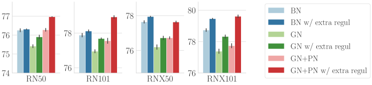
Figure 9: Effect of changing the choice of the extra regularization. Validation accuracies (%) of ResNets and ResNeXts trained on ImageNet with BN and GN, GN+PN, without extra regularization and with an extra regularization other than the one used in Table 7.

A.4 Results on CIFAR-10 and CIFAR-100

In this section, we report results on CIFAR with different sizes of ResNets: ResNet-20 (RN20), ResNet-32 (RN32), ResNet-44 (RN44), ResNet-56 (RN56), ResNet-110 (RN110).

We report results on CIFAR-10 in Table 15, and results on CIFAR-100 in Table 16. We further provide a visualization of these results in Figure 10.

While slightly underperforming BN on CIFAR-10, GN+PN tends to slightly outperform BN on CIFAR-100. As a possible reason, BN’s regularization could be more beneficial on the easy task of CIFAR-10 than on the harder task of CIFAR-100. To the extent that BN’s regularization can be seen as a reduction of the network’s effective capacity, such a reduction of the network’s effective capacity could be more harmful for tasks that require more capacity, i.e. for harder tasks.

Table 15: BN vs. GN, GN+PN on CIFAR-10. ResNets are trained with BN and GN, GN+PN. Results are formatted as X / Y with X, Y the validation accuracies (mean and $1\sigma$ interval in %) without and with extra regularization, respectively.

	RN20	RN32	RN44	RN56	RN110
BN	91.6$\pm$0.3 / 91.8$\pm$0.2	92.4$\pm$0.1 / 92.7$\pm$0.2	92.7$\pm$0.2 / 93.1$\pm$0.2	93.0$\pm$0.1 / 93.4$\pm$0.2	93.5$\pm$0.1 / 93.7$\pm$0.2
GN	90.8$\pm$0.2 / 90.7$\pm$0.1	91.5$\pm$0.2 / 91.5$\pm$0.1	91.8$\pm$0.2 / 92.0$\pm$0.1	92.2$\pm$0.2 / 92.2$\pm$0.2	92.6$\pm$0.2 / 92.9$\pm$0.3
GN+PN	91.4$\pm$0.2 / 91.6$\pm$0.3	92.3$\pm$0.2 / 92.5$\pm$0.2	92.8$\pm$0.2 / 92.9$\pm$0.2	92.9$\pm$0.2 / 93.2$\pm$0.2	93.2$\pm$0.1 / 93.6$\pm$0.1

Table 16: BN vs. GN, GN+PN on CIFAR-100. ResNets are trained with BN and GN, GN+PN. Results are formatted as in Table 15.

	RN20	RN32	RN44	RN56	RN110
BN	66.8$\pm$0.3 / 65.1$\pm$0.2	68.2$\pm$0.3 / 68.7$\pm$0.2	69.2$\pm$0.4 / 70.5$\pm$0.2	70.1$\pm$0.2 / 71.4$\pm$0.3	71.7$\pm$0.3 / 73.3$\pm$0.3
GN	65.0$\pm$0.3 / 61.7$\pm$0.3	66.5$\pm$0.4 / 65.3$\pm$0.4	67.3$\pm$0.6 / 67.0$\pm$0.3	67.8$\pm$0.4 / 68.1$\pm$0.5	69.5$\pm$0.3 / 70.2$\pm$0.4
GN+PN	66.3$\pm$0.4 / 66.7$\pm$0.2	67.8$\pm$0.4 / 69.5$\pm$0.2	68.9$\pm$0.3 / 70.8$\pm$0.4	69.8$\pm$0.3 / 71.7$\pm$0.4	71.4$\pm$0.2 / 73.1$\pm$0.4

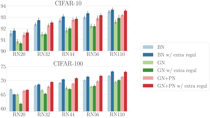
Figure 10: BN vs. GN, GN+PN. Validation accuracies (%) of ResNets trained on CIFAR-10 (top) and CIFAR-100 (bottom) with BN and GN, GN+PN, without and with extra regularization.

Appendix B Implementation of Proxy Norm

In this section, we provide a Tensorflow 1 implementation of the proxy-normalized activation step when PN’s additional parameters $\tilde{{\bm{\beta}}}^{l}$, $\tilde{{\bm{\gamma}}}^{l}$ are set to zero, i.e. omitted (cf Section 5).

⬇

import tensorflow as tf

import numpy as np

from scipy.special import erfinv

def uniformly_sampled_gaussian(num_rand):

rand = 2 * (np.arange(num_rand) + 0.5) / float(num_rand) - 1

return np.sqrt(2) * erfinv(rand)

def proxy_norm_act(y,

activation_fn=tf.nn.relu,

proxy_epsilon=0.03,

num_samples=256):

"""

TensorFlow 1 implementation of the proxy normalized activation step.

Following the same convention as in the main text of this paper,

the affine transform is applied in this step rather than in the normalization step.

:param y: 4D activation tensor after the normalization step

:param activation_fn: activation function

:param proxy_epsilon: PN’s numerical stability constant (should not be too low)

:param num_samples: number of samples in the proxy distribution

:return tilde_z: 4D activation tensor after the proxy-normalized activation step

"""

def create_channelwise_variable(name, init):

num_channels = int(y.get_shape()[-1])

return tf.get_variable(name,

dtype=y.dtype,

shape=[1, 1, 1, num_channels],

initializer=tf.constant_initializer(init))

# shift and scale parameters after the norm

beta = create_channelwise_variable(’beta’, 0.0)

gamma = create_channelwise_variable(’gamma’, 1.0)

# activation step

z = gamma * y + beta # affine transform

z = activation_fn(z) # activation function

# proxy normalization

proxy_y = tf.constant(uniformly_sampled_gaussian(num_samples), y.dtype)

proxy_y = tf.reshape(proxy_y, [num_samples, 1, 1, 1])

proxy_z = gamma * proxy_y + beta # affine transform on proxy distribution

proxy_z = activation_fn(proxy_z) # activation function on proxy distribution

# compute proxy statistics in float32

proxy_mean, proxy_var = tf.nn.moments(

tf.cast(proxy_z, tf.float32), axes=[0], keepdims=True)

proxy_mean = tf.cast(proxy_mean, y.dtype)

inv_proxy_std = tf.cast(tf.rsqrt(proxy_var + proxy_epsilon), y.dtype)

# normalize z according to proxy statistics

tilde_z = (z - proxy_mean) * inv_proxy_std

return tilde_z

Appendix C Proofs of results other than Theorems 1, 2, 3

C.1 Layer-wise power equals one

Proposition 1.

If $\sigma_{I_{{\mathbf{x}},c}}({\mathbf{x}}^{l})\neq 0$ for all ${\mathbf{x}}\in\mathcal{D}$ and $c\in\{1,\dots,C_{l}\}$, then it holds that $\mathcal{P}({\mathbf{y}}^{l})=1$ for any choice of $\operatorname{Norm}\in\{\operatorname{BN},\operatorname{LN},\operatorname{IN},\operatorname{GN}\}$.

Proof. The proof proceeds by distinguishing each case in $\operatorname{Norm}\in\{\operatorname{BN},\operatorname{LN},\operatorname{IN},\operatorname{GN}\}$.

Case of BN.

If we fix a channel $c$, the assumption $\sigma_{c}({\mathbf{x}}^{l})\neq 0$ implies that

$$\mathcal{P}_{c}({\mathbf{y}}^{l}) =\frac{\mathbb{E}_{{\mathbf{x}},\alpha}\Big{[}\big{(}{\mathbf{x}}^{l}_{\alpha,c}-\mu_{c}({\mathbf{x}}^{l})\big{)}^{2}\Big{]}}{\sigma_{c}({\mathbf{x}}^{l})^{2}}=\frac{\sigma_{c}({\mathbf{x}}^{l})^{2}}{\sigma_{c}({\mathbf{x}}^{l})^{2}}=1.$$

We immediately get $\mathcal{P}({\mathbf{y}}^{l})=\mathbb{E}_{c}\Big{[}\mathcal{P}_{c}({\mathbf{y}}^{l})\Big{]}=1$.

Case of GN.

Let us fix ${\mathbf{x}}\in\mathcal{D}$ and let us denote $\mathcal{G}_{g}$ for $g\in\{1,\dots,G\}$ the $G$ groups of channels and $I^{(g)}_{{\mathbf{x}}}=\{{\mathbf{x}},c\in\mathcal{G}_{g}\}$ for $g\in\{1,\dots,G\}$ the $G$ conditional sets of standardization.

The assumption $\sigma_{I^{(g)}_{{\mathbf{x}}}}({\mathbf{x}}^{l})\neq 0$ implies for any $g$ that

$$\mathcal{P}_{I^{(g)}_{{\mathbf{x}}}}({\mathbf{y}}^{l}) =\frac{\mathbb{E}_{\alpha,c|c\in\mathcal{G}_{g}}\Big{[}\big{(}{\mathbf{x}}^{l}_{\alpha,c}-\mu_{I^{(g)}_{{\mathbf{x}}}}({\mathbf{x}}^{l})\big{)}^{2}\Big{]}}{\sigma_{I^{(g)}_{{\mathbf{x}}}}({\mathbf{x}}^{l})^{2}}=\frac{\sigma_{I^{(g)}_{{\mathbf{x}}}}({\mathbf{x}}^{l})^{2}}{\sigma_{I^{(g)}_{{\mathbf{x}}}}({\mathbf{x}}^{l})^{2}}=1.$$

This implies

$$\mathcal{P}_{{\mathbf{x}}}({\mathbf{y}}^{l}) =\frac{1}{C_{l}}\sum_{c}\mathcal{P}_{{\mathbf{x}},c}({\mathbf{y}}^{l})=\frac{1}{C_{l}}\sum_{g}\sum_{c\in\mathcal{G}_{g}}\mathcal{P}_{{\mathbf{x}},c}({\mathbf{y}}^{l})$$

$$=\frac{1}{C_{l}}\sum_{g}|\mathcal{G}_{g}|\mathcal{P}_{I^{(g)}_{{\mathbf{x}}}}({\mathbf{y}}^{l})=\frac{1}{C_{l}}\sum_{g}|\mathcal{G}_{g}|=1,$$

where we used $\mathcal{P}_{I^{(g)}_{{\mathbf{x}}}}({\mathbf{y}}^{l})=\frac{1}{|\mathcal{G}_{g}|}\sum_{c\in\mathcal{G}_{g}}\mathcal{P}_{{\mathbf{x}},c}({\mathbf{y}}^{l})$.

We immediately get $\mathcal{P}({\mathbf{y}}^{l})=\mathbb{E}_{\mathbf{x}}\Big{[}\mathcal{P}_{\mathbf{x}}({\mathbf{y}}^{l})\Big{]}=1$.

Cases of LN and IN.

The cases of LN and IN immediately follow from the cases of GN with $G=1$ group and $G=C_{l}$ groups. ∎

C.2 Channel-wise collapse implies channel-wise linearity

Some additional notations are required in this section. We denote $\Theta^{l}\equiv({\bm{\omega}}^{1},{\bm{\beta}}^{1},{\bm{\gamma}}^{1},\dots,{\bm{\omega}}^{l},{\bm{\beta}}^{l},{\bm{\gamma}}^{l})$ the aggregated model parameters up to layer $l$.

We further define the linearized post-activations $\widetilde{{\mathbf{z}}}^{l}$ as

$$\forall\alpha,c:\quad \widetilde{{\mathbf{z}}}^{l}_{\alpha,c}=\widetilde{\lambda}_{c}\tilde{{\mathbf{y}}}^{l}_{\alpha,c},$$ (8)

$$\forall c:\quad \widetilde{\lambda}_{c}=\operatorname*{arg\,min}_{\lambda_{c}}\mathbb{E}_{{\mathbf{x}},\alpha}\Big{[}\big{(}{\mathbf{z}}^{l}_{\alpha,c}-\lambda_{c}\tilde{{\mathbf{y}}}^{l}_{\alpha,c}\big{)}^{2}\Big{]}=\operatorname*{arg\,min}_{\lambda_{c}}\mathbb{E}_{{\mathbf{x}},\alpha}\Big{[}\big{(}\phi(\tilde{{\mathbf{y}}}^{l}_{\alpha,c})-\lambda_{c}\tilde{{\mathbf{y}}}^{l}_{\alpha,c}\big{)}^{2}\Big{]}.$$ (9)

The linearized post-activations $\widetilde{{\mathbf{z}}}^{l}$ are the channel-wise linear best-fit of ${\mathbf{z}}^{l}=\phi(\tilde{{\mathbf{y}}}^{l})$ using $\tilde{{\mathbf{y}}}^{l}$.

We start by proving that the inequality $\mathcal{P}_{c}(\tilde{{\mathbf{y}}}^{l})-\mathcal{P}^{(1)}_{c}(\tilde{{\mathbf{y}}}^{l})\leq\tilde{\eta}\mathcal{P}^{(1)}_{c}(\tilde{{\mathbf{y}}}^{l})$ for sufficiently small $\tilde{\eta}$ implies channel-wise linearity (Proposition 2). We then prove that the inequality $\mathcal{P}_{c}(\tilde{{\mathbf{y}}}^{l})-\mathcal{P}^{(1)}_{c}(\tilde{{\mathbf{y}}}^{l})\leq\widetilde{\eta}\mathcal{P}_{c}(\tilde{{\mathbf{y}}}^{l})$ for sufficiently small $\widetilde{\eta}$ implies channel-wise-linearity (Proposition 3).

Proposition 2.

If we fix some $d\in{\mathbb{N}}^{*}$, there exists $\tilde{\eta}>0$ such that for any choice of $(\phi,H,W,\mathcal{D},\Theta^{l})$, it holds that

$$\Big{(}HW|\mathcal{D}|=d\Big{)}\land\Big{(}\mathcal{P}_{c}(\tilde{{\mathbf{y}}}^{l})-\mathcal{P}^{(1)}_{c}(\tilde{{\mathbf{y}}}^{l})\leq\tilde{\eta}\mathcal{P}^{(1)}_{c}(\tilde{{\mathbf{y}}}^{l})\Big{)}\implies{\mathbf{z}}^{l}_{\alpha,c}=\widetilde{{\mathbf{z}}}^{l}_{\alpha,c}\;\forall{\mathbf{x}},\alpha,$$

where $\widetilde{{\mathbf{z}}}^{l}$ are the linearized post-activations defined in Eq. (8), (9) and $\land$ is the logical and.

Proof. Any positive homogeneous $\phi$ satisfies $\phi(r)=r\phi(1)$ and $\phi(-r)=r\phi(-1)$ for any $r\geq 0$. This means that any positive homogeneous $\phi$ is: (i) fully determined by its values at $+1$ and $-1$; (ii) linear on the intervals $(-\infty,0]$ and $[0,+\infty)$.

A sufficient condition for the linearity with respect to ${\mathbf{x}},\alpha$ in channel $c$ is therefore a constant sign of $\tilde{{\mathbf{y}}}^{l}_{\alpha,c}$ for all ${\mathbf{x}},\alpha$. Let us see that this constant sign is implied by a sufficiently severe channel-wise collapse.

We start by proving the result with the two distinct conditionalities: (i) $\sigma_{c}(\tilde{{\mathbf{y}}}^{l})=0$ and (ii) $\sigma_{c}(\tilde{{\mathbf{y}}}^{l})>0$.

Conditionality $\sigma_{c}(\tilde{{\mathbf{y}}}^{l})=0$.

If $\sigma_{c}(\tilde{{\mathbf{y}}}^{l})=0$, then $\tilde{{\mathbf{y}}}^{l}_{\alpha,c}=\mu_{c}(\tilde{{\mathbf{y}}}^{l})$, $\forall{\mathbf{x}},\alpha$.

Let us then define $\lambda_{c}$ such that $\lambda_{c}=0$ if $\mu_{c}(\tilde{{\mathbf{y}}}^{l})=0$, and $\lambda_{c}=\frac{\phi(\mu_{c}(\tilde{{\mathbf{y}}}^{l}))}{\mu_{c}(\tilde{{\mathbf{y}}}^{l})}$ otherwise.

For any choice of positive homogeneous $\phi$, it holds that $\phi(0)=0$. Combined with the definition of $\lambda_{c}$, this implies $\phi(\mu_{c}(\tilde{{\mathbf{y}}}^{l}))=\lambda_{c}\mu_{c}(\tilde{{\mathbf{y}}}^{l})$ and thus $\forall{\mathbf{x}},\alpha$:

$${\mathbf{z}}^{l}_{\alpha,c}=\phi(\tilde{{\mathbf{y}}}^{l}_{\alpha,c})=\phi(\mu_{c}(\tilde{{\mathbf{y}}}^{l}))=\lambda_{c}\mu_{c}(\tilde{{\mathbf{y}}}^{l})=\lambda_{c}\tilde{{\mathbf{y}}}^{l}_{\alpha,c}.$$

Given the definition of the linearized post-activations $\widetilde{{\mathbf{z}}}^{l}$, this means

$$\mathbb{E}_{{\mathbf{x}},\alpha}\Big{[}\big{(}{\mathbf{z}}^{l}_{\alpha,c}-\widetilde{{\mathbf{z}}}^{l}_{\alpha,c}\big{)}^{2}\Big{]}\leq\mathbb{E}_{{\mathbf{x}},\alpha}\Big{[}\big{(}{\mathbf{z}}^{l}_{\alpha,c}-\lambda_{c}\tilde{{\mathbf{y}}}^{l}_{\alpha,c}\big{)}^{2}\Big{]}=0.$$

This immediately implies $\forall{\mathbf{x}},\alpha$: ${\mathbf{z}}^{l}_{\alpha,c}=\widetilde{{\mathbf{z}}}^{l}_{\alpha,c}$. Thus, for any $(\phi,H,W,\mathcal{D},\Theta^{l})$ such that $\sigma_{c}(\tilde{{\mathbf{y}}}^{l})=0$, it holds that $\forall{\mathbf{x}},\alpha$: ${\mathbf{z}}^{l}_{\alpha,c}=\widetilde{{\mathbf{z}}}^{l}_{\alpha,c}$.

More concisely, it holds for any choice of $(\phi,H,W,\mathcal{D},\Theta^{l})$ that

$$\sigma_{c}(\tilde{{\mathbf{y}}}^{l})=0\implies{\mathbf{z}}^{l}_{\alpha,c}=\widetilde{{\mathbf{z}}}^{l}_{\alpha,c}\;\forall{\mathbf{x}},\alpha.$$ (10)

Conditionality $\sigma_{c}(\tilde{{\mathbf{y}}}^{l})>0$.

We start by fixing $(\phi,H,W,\mathcal{D},\Theta^{l})$. For any given $k>0$, Chebyshev’s inequality implies

$$\mathbb{P}_{{\mathbf{x}},\alpha}\Big{[}|\tilde{{\mathbf{y}}}^{l}_{\alpha,c}-\mu_{c}(\tilde{{\mathbf{y}}}^{l})|\geq k\sigma_{c}(\tilde{{\mathbf{y}}}^{l})\Big{]} \leq\frac{1}{k^{2}},$$

$$\mathbb{P}_{{\mathbf{x}},\alpha}\Big{[}\big{(}\tilde{{\mathbf{y}}}^{l}_{\alpha,c}-\mu_{c}(\tilde{{\mathbf{y}}}^{l})\big{)}^{2}\geq k^{2}\sigma_{c}(\tilde{{\mathbf{y}}}^{l})^{2}\Big{]} \leq\frac{1}{k^{2}}.$$

Thus, if $\mathcal{P}_{c}(\tilde{{\mathbf{y}}}^{l})-\mathcal{P}^{(1)}_{c}(\tilde{{\mathbf{y}}}^{l})\leq\eta\mathcal{P}^{(1)}_{c}(\tilde{{\mathbf{y}}}^{l})$ for some $\eta>0$, it holds for any given $k>0$ that

$$1-\frac{1}{k^{2}} \leq\mathbb{P}_{{\mathbf{x}},\alpha}\Big{[}\big{(}\tilde{{\mathbf{y}}}^{l}_{\alpha,c}-\mu_{c}(\tilde{{\mathbf{y}}}^{l})\big{)}^{2}<k^{2}\sigma_{c}(\tilde{{\mathbf{y}}}^{l})^{2}\Big{]}=\mathbb{P}_{{\mathbf{x}},\alpha}\Big{[}\big{(}\tilde{{\mathbf{y}}}^{l}_{\alpha,c}-\mu_{c}(\tilde{{\mathbf{y}}}^{l})\big{)}^{2}<k^{2}\big{(}\mathcal{P}_{c}(\tilde{{\mathbf{y}}}^{l})-\mathcal{P}^{(1)}_{c}(\tilde{{\mathbf{y}}}^{l})\big{)}\Big{]}$$

$$\leq\mathbb{P}_{{\mathbf{x}},\alpha}\Big{[}\big{(}\tilde{{\mathbf{y}}}^{l}_{\alpha,c}-\mu_{c}(\tilde{{\mathbf{y}}}^{l})\big{)}^{2}<k^{2}\eta\mathcal{P}^{(1)}_{c}(\tilde{{\mathbf{y}}}^{l})\Big{]}=\mathbb{P}_{{\mathbf{x}},\alpha}\Big{[}\big{(}\tilde{{\mathbf{y}}}^{l}_{\alpha,c}-\mu_{c}(\tilde{{\mathbf{y}}}^{l})\big{)}^{2}<k^{2}\eta\mu_{c}(\tilde{{\mathbf{y}}}^{l})^{2}\Big{]}$$

$$\leq\mathbb{P}_{{\mathbf{x}},\alpha}\Big{[}|\tilde{{\mathbf{y}}}^{l}_{\alpha,c}-\mu_{c}(\tilde{{\mathbf{y}}}^{l})|<k\sqrt{\eta}|\mu_{c}(\tilde{{\mathbf{y}}}^{l})|\Big{]}.$$

Choosing $k=\frac{1}{\sqrt{\eta}}$, we get

$$\mathbb{P}_{{\mathbf{x}},\alpha}\Big{[}|\tilde{{\mathbf{y}}}^{l}_{\alpha,c}-\mu_{c}(\tilde{{\mathbf{y}}}^{l})|\geq|\mu_{c}(\tilde{{\mathbf{y}}}^{l})|\Big{]}\leq\eta.$$

Now if we suppose that $\eta$ is such that $\frac{1}{HW|\mathcal{D}|}>\eta>0$, we get

$$\mathbb{P}_{{\mathbf{x}},\alpha}\Big{[}|\tilde{{\mathbf{y}}}^{l}_{\alpha,c}-\mu_{c}(\tilde{{\mathbf{y}}}^{l})|\geq|\mu_{c}(\tilde{{\mathbf{y}}}^{l})|\Big{]}<\frac{1}{HW|\mathcal{D}|}.$$ (11)

Eq. (11) could not hold if there existed ${\mathbf{x}}\in\mathcal{D}$ and $\alpha\in\{1,\dots,H\}\times\{1,\dots,W\}$ such that $|\tilde{{\mathbf{y}}}^{l}_{\alpha,c}-\mu_{c}(\tilde{{\mathbf{y}}}^{l})|\geq|\mu_{c}(\tilde{{\mathbf{y}}}^{l})|$. Consequently, $|\tilde{{\mathbf{y}}}^{l}_{\alpha,c}-\mu_{c}(\tilde{{\mathbf{y}}}^{l})|<|\mu_{c}(\tilde{{\mathbf{y}}}^{l})|$ for all ${\mathbf{x}},\alpha$, implying that there exists a tensor ${\mathbf{r}}^{l}\in\mathbb{R}^{H\times W\times C_{l}}$ that implicitly depends on ${\mathbf{x}}$ such that $\forall{\mathbf{x}},\alpha$:

$$\tilde{{\mathbf{y}}}^{l}_{\alpha,c}={\mathbf{r}}^{l}_{\alpha,c}\mu_{c}(\tilde{{\mathbf{y}}}^{l}),\qquad{\mathbf{r}}^{l}_{\alpha,c}\geq 0.$$ (12)

Now if we combine $\sigma_{c}(\tilde{{\mathbf{y}}}^{l})>0$ with $\mathcal{P}_{c}(\tilde{{\mathbf{y}}}^{l})-\mathcal{P}^{(1)}_{c}(\tilde{{\mathbf{y}}}^{l})\leq\eta\mathcal{P}^{(1)}_{c}(\tilde{{\mathbf{y}}}^{l})$, we deduce that $\mathcal{P}^{(1)}_{c}(\tilde{{\mathbf{y}}}^{l})>0$ and thus that $\mu_{c}(\tilde{{\mathbf{y}}}^{l})\neq 0$. Combining this with Eq. (12), we get $\forall{\mathbf{x}},\alpha$:

$${\mathbf{z}}^{l}_{\alpha,c}=\phi(\tilde{{\mathbf{y}}}^{l}_{\alpha,c})={\mathbf{r}}^{l}_{\alpha,c}\phi(\mu_{c}(\tilde{{\mathbf{y}}}^{l}))=\frac{\phi(\mu_{c}(\tilde{{\mathbf{y}}}^{l}))}{\mu_{c}(\tilde{{\mathbf{y}}}^{l})}{\mathbf{r}}^{l}_{\alpha,c}\mu_{c}(\tilde{{\mathbf{y}}}^{l})=\lambda_{c}\tilde{{\mathbf{y}}}^{l}_{\alpha,c},$$

where we defined $\lambda_{c}\equiv\frac{\phi(\mu_{c}(\tilde{{\mathbf{y}}}^{l}))}{\mu_{c}(\tilde{{\mathbf{y}}}^{l})}$.

Given the definition of the linearized post-activations $\widetilde{{\mathbf{z}}}^{l}$, this means

$$\mathbb{E}_{{\mathbf{x}},\alpha}\Big{[}\big{(}{\mathbf{z}}^{l}_{\alpha,c}-\widetilde{{\mathbf{z}}}^{l}_{\alpha,c}\big{)}^{2}\Big{]}\leq\mathbb{E}_{{\mathbf{x}},\alpha}\Big{[}\big{(}{\mathbf{z}}^{l}_{\alpha,c}-\lambda_{c}\tilde{{\mathbf{y}}}^{l}_{\alpha,c}\big{)}^{2}\Big{]}=0.$$

This immediately implies $\forall{\mathbf{x}},\alpha$: ${\mathbf{z}}^{l}_{\alpha,c}=\widetilde{{\mathbf{z}}}^{l}_{\alpha,c}$.

Thus, if we fix some $d\in{\mathbb{N}}^{*}$ and if we define $\tilde{\eta}=\frac{1}{2d}$, it holds for any choice of $(\phi,H,W,\mathcal{D},\Theta^{l})$ such that (i) $HW|\mathcal{D}|=d$, (ii) $\mathcal{P}_{c}(\tilde{{\mathbf{y}}}^{l})-\mathcal{P}^{(1)}_{c}(\tilde{{\mathbf{y}}}^{l})\leq\tilde{\eta}\mathcal{P}^{(1)}_{c}(\tilde{{\mathbf{y}}}^{l})$, (iii) $\sigma_{c}(\tilde{{\mathbf{y}}}^{l})>0$, that $\forall{\mathbf{x}},\alpha$: ${\mathbf{z}}^{l}_{\alpha,c}=\widetilde{{\mathbf{z}}}^{l}_{\alpha,c}$.

More concisely, it holds for any choice of $(\phi,H,W,\mathcal{D},\Theta^{l})$ that

$$\Big{(}HW|\mathcal{D}|=d\Big{)}\land\Big{(}\mathcal{P}_{c}(\tilde{{\mathbf{y}}}^{l})-\mathcal{P}^{(1)}_{c}(\tilde{{\mathbf{y}}}^{l})\leq\tilde{\eta}\mathcal{P}^{(1)}_{c}(\tilde{{\mathbf{y}}}^{l})\Big{)}\land\Big{(}\sigma_{c}(\tilde{{\mathbf{y}}}^{l})>0\Big{)}\implies{\mathbf{z}}^{l}_{\alpha,c}=\widetilde{{\mathbf{z}}}^{l}_{\alpha,c}\;\forall{\mathbf{x}},\alpha.$$ (13)

General case.

To wrap up, if we fix some $d\in{\mathbb{N}}^{*}$ and if we reuse the definition $\tilde{\eta}=\frac{1}{2d}$, it holds for any choice of $(\phi,H,W,\mathcal{D},\Theta^{l})$ that

$$\Big{(}HW|\mathcal{D}|=d\Big{)}\land\Big{(}\mathcal{P}_{c}(\tilde{{\mathbf{y}}}^{l})-\mathcal{P}^{(1)}_{c}(\tilde{{\mathbf{y}}}^{l})\leq\tilde{\eta}\mathcal{P}^{(1)}_{c}(\tilde{{\mathbf{y}}}^{l})\Big{)}$$

$$\qquad\implies\Bigg{(}\Big{(}HW|\mathcal{D}|=d\Big{)}\land\Big{(}\mathcal{P}_{c}(\tilde{{\mathbf{y}}}^{l})-\mathcal{P}^{(1)}_{c}(\tilde{{\mathbf{y}}}^{l})\leq\tilde{\eta}\mathcal{P}^{(1)}_{c}(\tilde{{\mathbf{y}}}^{l})\Big{)}\land\Big{(}\sigma_{c}(\tilde{{\mathbf{y}}}^{l})=0\Big{)}\Bigg{)}$$

$$\qquad\qquad\lor\Bigg{(}\Big{(}HW|\mathcal{D}|=d\Big{)}\land\Big{(}\mathcal{P}_{c}(\tilde{{\mathbf{y}}}^{l})-\mathcal{P}^{(1)}_{c}(\tilde{{\mathbf{y}}}^{l})\leq\tilde{\eta}\mathcal{P}^{(1)}_{c}(\tilde{{\mathbf{y}}}^{l})\Big{)}\land\Big{(}\sigma_{c}(\tilde{{\mathbf{y}}}^{l})>0\Big{)}\Bigg{)}$$

$$\qquad\implies\Big{(}{\mathbf{z}}^{l}_{\alpha,c}=\widetilde{{\mathbf{z}}}^{l}_{\alpha,c}\;\forall{\mathbf{x}},\alpha\Big{)}\lor\Big{(}{\mathbf{z}}^{l}_{\alpha,c}=\widetilde{{\mathbf{z}}}^{l}_{\alpha,c}\;\forall{\mathbf{x}},\alpha\Big{)}$$ (14)

$$\qquad\implies\Big{(}{\mathbf{z}}^{l}_{\alpha,c}=\widetilde{{\mathbf{z}}}^{l}_{\alpha,c}\;\forall{\mathbf{x}},\alpha\Big{)},$$

where Eq. (14) is obtained using Eq. (10) and Eq. (13) and $\land$, $\lor$ are the logical and and or. ∎

Proposition 3.

If we fix some $d\in{\mathbb{N}}^{*}$, there exists $\widetilde{\eta}>0$ such that for any choice of $(\phi,H,W,\mathcal{D},\Theta^{l})$, it holds that

$$\Big{(}HW|\mathcal{D}|=d\Big{)}\land\Big{(}\mathcal{P}_{c}(\tilde{{\mathbf{y}}}^{l})-\mathcal{P}^{(1)}_{c}(\tilde{{\mathbf{y}}}^{l})\leq\widetilde{\eta}\mathcal{P}_{c}(\tilde{{\mathbf{y}}}^{l})\Big{)}\implies{\mathbf{z}}^{l}_{\alpha,c}=\widetilde{{\mathbf{z}}}^{l}_{\alpha,c}\;\forall{\mathbf{x}},\alpha,$$

where $\widetilde{{\mathbf{z}}}^{l}$ are the linearized post-activations defined in Eq. (8), (9) and $\land$ is the logical and.

Proof. We start by noting that for any $1>\eta>0$:

$$\mathcal{P}_{c}(\tilde{{\mathbf{y}}}^{l})-\mathcal{P}^{(1)}_{c}(\tilde{{\mathbf{y}}}^{l})\leq\eta\mathcal{P}_{c}(\tilde{{\mathbf{y}}}^{l}) \iff\mathcal{P}_{c}(\tilde{{\mathbf{y}}}^{l})-\mathcal{P}^{(1)}_{c}(\tilde{{\mathbf{y}}}^{l})\leq\eta\Big{(}\mathcal{P}_{c}(\tilde{{\mathbf{y}}}^{l})-\mathcal{P}^{(1)}_{c}(\tilde{{\mathbf{y}}}^{l})+\mathcal{P}^{(1)}_{c}(\tilde{{\mathbf{y}}}^{l})\Big{)}$$

$$\iff\mathcal{P}_{c}(\tilde{{\mathbf{y}}}^{l})-\mathcal{P}^{(1)}_{c}(\tilde{{\mathbf{y}}}^{l})\leq\frac{\eta}{1-\eta}\mathcal{P}^{(1)}_{c}(\tilde{{\mathbf{y}}}^{l}).$$

Thus, if we fix some $d\in{\mathbb{N}}^{*}$ and if we define $\tilde{\eta}=\frac{1}{2d}$ and $\widetilde{\eta}=\frac{\tilde{\eta}}{1+\tilde{\eta}}$, it holds for any choice of $(\phi,H,W,\mathcal{D},\Theta^{l})$ that

$$\Big{(}HW|\mathcal{D}|=d\Big{)}\land\Big{(}\mathcal{P}_{c}(\tilde{{\mathbf{y}}}^{l})-\mathcal{P}^{(1)}_{c}(\tilde{{\mathbf{y}}}^{l})\leq\widetilde{\eta}\mathcal{P}_{c}(\tilde{{\mathbf{y}}}^{l})\Big{)}$$

$$\qquad\iff\Big{(}HW|\mathcal{D}|=d\Big{)}\land\Big{(}\mathcal{P}_{c}(\tilde{{\mathbf{y}}}^{l})-\mathcal{P}^{(1)}_{c}(\tilde{{\mathbf{y}}}^{l})\leq\frac{\widetilde{\eta}}{1-\widetilde{\eta}}\mathcal{P}^{(1)}_{c}(\tilde{{\mathbf{y}}}^{l})\Big{)}$$

$$\qquad\iff\Big{(}HW|\mathcal{D}|=d\Big{)}\land\Big{(}\mathcal{P}_{c}(\tilde{{\mathbf{y}}}^{l})-\mathcal{P}^{(1)}_{c}(\tilde{{\mathbf{y}}}^{l})\leq\tilde{\eta}\mathcal{P}^{(1)}_{c}(\tilde{{\mathbf{y}}}^{l})\Big{)}$$

$$\qquad\implies\Big{(}{\mathbf{z}}^{l}_{\alpha,c}=\widetilde{{\mathbf{z}}}^{l}_{\alpha,c}\;\forall{\mathbf{x}},\alpha\Big{)},$$ (15)

where Eq. (15) is obtained using Proposition 2 and $\land$ is the logical and. ∎

C.3 Alteration of expressivity with IN

In this section, we first prove that, for any dataset $\mathcal{D}$, networks without normalization can express mappings arbitrarily close to the identity (Proposition 4). We then prove that, in general, networks with IN cannot express mappings arbitrarily close to the identity (Proposition 5).

Proposition 4.

Lift any assumptions on $\phi$ and suppose instead that $\phi$ is non-polynomial. Further suppose that each layer $l$ up to depth $L$ implements the following two steps $\forall\alpha,c$:

$${\mathbf{y}}^{l}_{\alpha,c} =({\bm{\omega}}^{l}\ast{\mathbf{z}}^{l-1})_{\alpha,c}+{\mathbf{b}}^{l}_{c},$$ (16)

$${\mathbf{z}}^{l}_{\alpha,c} =\phi\big{(}{\mathbf{y}}^{l}_{\alpha,c}\big{)},$$ (17)

where ${\mathbf{z}}^{0}\equiv{\mathbf{x}}$, and ${\bm{\omega}}^{l}\in\mathbb{R}^{K_{l}\times K_{l}\times C_{l-1}\times C_{l}}$ and ${\mathbf{b}}^{l}\in\mathbb{R}^{C_{l}}$ are the weights and biases at layer $l$.

Now fix a layer $l\in\{1,\dots,L\}$, the spatial extents $H$, $W$, the widths $C_{0}$, $C_{l}$ assumed equal at layer $0$ and layer $l$, and the dataset $\mathcal{D}$. Further denote $\Phi_{l}$ the network mapping from ${\mathbf{x}}$ to ${\mathbf{y}}^{l}$ such that ${\mathbf{y}}^{l}=\Phi_{l}({\mathbf{x}})$.

Then for any $\epsilon>0$, there exists a choice of intermediate widths $(C_{k})_{1\leq k<l}$ and model parameters $({\bm{\omega}}^{1},{\mathbf{b}}^{1},\dots,{\bm{\omega}}^{l},{\mathbf{b}}^{l})$ such that

$$\max_{{\mathbf{x}}\in\mathcal{D}}||\Phi_{l}({\mathbf{x}})-{\mathbf{x}}||\leq\epsilon.$$

Proof. The proof proceeds in multiple steps of increasing generality.

Case of unit spatial extent of activations and kernels.

When $H$, $W$ are equal to $1$ and $K_{k}$ is equal to one at every layer $k$, the propagation of Eq. (16), (17) becomes strictly equivalent to the propagation in a fully-connected network.

If $l$ is the first layer in the network ($l=1$), we may obtain the strict equality $\Phi_{l}=\operatorname*{identity}$ by choosing the reshaped matricial version ${\bm{W}}^{l}\in\mathbb{R}^{C_{0}\times C_{l}}$ of ${\bm{\omega}}^{l}$ as the identity and ${\mathbf{b}}^{l}$ as zero.

Otherwise ($l\geq 2$), we may apply the universal approximation theorem [91]. Given the assumption of non-polynomial activation function $\phi$, this means that for any $\epsilon>0$, there exists a choice of intermediate widths $(C_{k})_{1\leq k<l}$ and model parameters $({\bm{\omega}}^{1},{\mathbf{b}}^{1},\dots,{\bm{\omega}}^{l},{\mathbf{b}}^{l})$ such that

$$\max_{{\mathbf{x}}\in\mathcal{D}}||\Phi_{l}({\mathbf{x}})-{\mathbf{x}}||\leq\epsilon.$$ (18)

Case of unit spatial extent of kernels.

When $K_{k}$ is equal to one at every layer $k$, the propagation of Eq. (16), (17) occurs strictly independently for each spatial position $\alpha$.

Let us then consider a neural network that takes an input $\bar{{\mathbf{x}}}\in\mathbb{R}^{1\times 1\times C_{0}}$ and provides $\bar{{\mathbf{y}}}^{l}$, $\bar{{\mathbf{z}}}^{l}$ at every layer $l$ by implementing the same steps as Eq. (16), (17). Let us denote $\Psi_{l}$ the network mapping from $\bar{{\mathbf{x}}}$ to $\bar{{\mathbf{y}}}^{l}$ such that $\bar{{\mathbf{y}}}^{l}=\Psi_{l}(\bar{{\mathbf{x}}})$. And let us further denote $\overline{\mathcal{D}}=\{\bar{{\mathbf{x}}}^{({\mathbf{x}},\alpha)}\}_{{\mathbf{x}}\in\mathcal{D},\alpha\in\{1,\dots,H\}\times\{1,\dots,W\}}$, where $\bar{{\mathbf{x}}}^{({\mathbf{x}},\alpha)}\in\mathbb{R}^{1\times 1\times C_{0}}$ denotes the reshaped version of ${\mathbf{x}}_{\alpha,:}\in\mathbb{R}^{C_{0}}$ for any ${\mathbf{x}}$, $\alpha$.

If we fix any $\epsilon>0$ and if we apply Eq. (18) from the previous case with $\frac{1}{\sqrt{HW}}\epsilon$, we get that there exists a choice of intermediate widths $(C_{k})_{1\leq k<l}$ and model parameters $({\bm{\omega}}^{1},{\mathbf{b}}^{1},\dots,{\bm{\omega}}^{l},{\mathbf{b}}^{l})$ such that

$$\max_{\bar{{\mathbf{x}}}\in\overline{\mathcal{D}}}||\Psi_{l}(\bar{{\mathbf{x}}})-\bar{{\mathbf{x}}}||=\max_{{\mathbf{x}}\in\mathcal{D},\alpha\in\{1,\dots,H\}\times\{1,\dots,W\}}||\Psi_{l}(\bar{{\mathbf{x}}}^{({\mathbf{x}},\alpha)})-\bar{{\mathbf{x}}}^{({\mathbf{x}},\alpha)}||\leq\frac{1}{\sqrt{HW}}\epsilon.$$ (19)

Let us then fix $(C_{k})_{1\leq k<l}$ and $({\bm{\omega}}^{1},{\mathbf{b}}^{1},\dots,{\bm{\omega}}^{l},{\mathbf{b}}^{l})$ such that Eq. (19) holds.

Due to the independence of spatial positions, the mapping $\Phi_{l}$ is such that $\Phi_{l}({\mathbf{x}})_{\alpha,:}$ is a reshaped version of $\Psi_{l}(\bar{{\mathbf{x}}}^{({\mathbf{x}},\alpha)})$ for any ${\mathbf{x}}$, $\alpha$. This means that $\forall{\mathbf{x}}\in\mathcal{D}$ and $\forall\alpha\in\{1,\dots,H\}\times\{1,\dots,W\}$:

$$||\Phi_{l}({\mathbf{x}})_{\alpha,:}-{\mathbf{x}}_{\alpha,:}|| =||\Psi_{l}(\bar{{\mathbf{x}}}^{({\mathbf{x}},\alpha)})-\bar{{\mathbf{x}}}^{({\mathbf{x}},\alpha)}||\leq\frac{1}{\sqrt{HW}}\epsilon,$$

$$||\Phi_{l}({\mathbf{x}})-{\mathbf{x}}||^{2} =\sum_{\alpha\in\{1,\dots,H\}\times\{1,\dots,W\}}||\Phi_{l}({\mathbf{x}})_{\alpha,:}-{\mathbf{x}}_{\alpha,:}||^{2}\leq\sum_{\alpha\in\{1,\dots,H\}\times\{1,\dots,W\}}\frac{1}{HW}\epsilon^{2}\leq\epsilon^{2}.$$

This immediately implies

$$\max_{{\mathbf{x}}\in\mathcal{D}}||\Phi_{l}({\mathbf{x}})-{\mathbf{x}}||\leq\epsilon.$$

General case.

Let us consider the neural network that takes ${\mathbf{x}}\in\mathcal{D}$ as input and provides $\bar{{\mathbf{y}}}^{l}$, $\bar{{\mathbf{z}}}^{l}$ at every layer $l$ by implementing Eq. (16), (17) with weights $\bar{{\bm{\omega}}}^{l}\in\mathbb{R}^{1\times 1\times C_{l-1}\times C_{l}}$, biases $\bar{{\mathbf{b}}}^{l}\in\mathbb{R}^{C_{l}}$ and activation function $\phi$. Let us then denote $\Psi_{l}$ the network mapping from ${\mathbf{x}}$ to $\bar{{\mathbf{y}}}^{l}$ such that $\bar{{\mathbf{y}}}^{l}=\Psi_{l}({\mathbf{x}})$.

If we fix any $\epsilon>0$, we get from the previous case that there exists a choice of intermediate widths $(C_{k})_{1\leq k<l}$ and model parameters $(\bar{{\bm{\omega}}}^{1},\bar{{\mathbf{b}}}^{1},\dots,\bar{{\bm{\omega}}}^{l},\bar{{\mathbf{b}}}^{l})$ such that

$$\max_{{\mathbf{x}}\in\mathcal{D}}||\Psi_{l}({\mathbf{x}})-{\mathbf{x}}||\leq\epsilon.$$ (20)

Let us then fix $(C_{k})_{1\leq k<l}$ and $(\bar{{\bm{\omega}}}^{1},\bar{{\mathbf{b}}}^{1},\dots,\bar{{\bm{\omega}}}^{l},\bar{{\mathbf{b}}}^{l})$ such that Eq. (20) holds. Let us further define the weights and biases ${\bm{\omega}}^{k}$, ${\mathbf{b}}^{k}$ at each layer $k$ such that $\forall h,w,c,c^{\prime}$:

$${\bm{\omega}}^{k}_{h,w,c,c^{\prime}} \equiv\left\{\begin{array}[]{cc}&\text{if the multi-index $(h,w,c,c^{\prime})$ in the weights}\\ \bar{{\bm{\omega}}}^{k}_{1,1,c,c^{\prime}}&\text{associates spatial positions $\alpha$ in the convolution input ${\mathbf{z}}^{l-1}_{\alpha,c}$}\\ &\text{to the same spatial positions $\alpha$ in the convolution output ${\mathbf{y}}^{l}_{\alpha,c^{\prime}}$},\\ \\ 0&\text{otherwise,}\end{array}\right.$$

$${\mathbf{b}}^{k}_{c^{\prime}} \equiv\bar{{\mathbf{b}}}^{k}_{c^{\prime}}.$$

Then it holds that $\Phi_{l}=\Psi_{l}$, which in turn implies

$$\max_{{\mathbf{x}}\in\mathcal{D}}||\Phi_{l}({\mathbf{x}})-{\mathbf{x}}||\leq\epsilon.$$ ∎

Proposition 5.

Suppose that the neural network implements Eq. (2), (3), (4) in every layer up to depth $L$ and suppose $\operatorname{Norm}=\operatorname{IN}$.

Further fix a layer $l\in\{1,\dots,L\}$, the spatial extents $H$, $W$, the widths $C_{0}$, $C_{l}$ assumed equal at layer $0$ and layer $l$, and any dataset $\mathcal{D}$ such that there exists at least one channel in which the inputs of $\mathcal{D}$ do not all share the same statistics of instance mean, i.e.

$$\exists c,\;\exists{\mathbf{x}}^{\prime},{\mathbf{x}}^{\prime\prime}\in\mathcal{D}:\qquad\mathbb{E}_{\alpha}[{\mathbf{x}}^{\prime}_{\alpha,c}]\neq\mathbb{E}_{\alpha}[{\mathbf{x}}^{\prime\prime}_{\alpha,c}].$$

Then there exists $\epsilon>0$ such that for any choice of intermediate widths $(C_{k})_{1\leq k<l}$ and model parameters $({\bm{\omega}}^{1},{\bm{\beta}}^{1},{\bm{\gamma}}^{1},\dots,{\bm{\omega}}^{l},{\bm{\beta}}^{l},{\bm{\gamma}}^{l})$, it holds that

$$\max_{{\mathbf{x}}\in\mathcal{D}}||\Phi_{l}({\mathbf{x}})-{\mathbf{x}}||>\epsilon,$$

where $\Phi_{l}$ denotes the network mapping from ${\mathbf{x}}$ to $\tilde{{\mathbf{y}}}^{l}$ such that $\tilde{{\mathbf{y}}}^{l}=\Phi_{l}({\mathbf{x}})$, $\forall{\mathbf{x}}$.

Proof. Let us proceed by contradiction and suppose that for any $\epsilon>0$, there exists a choice of intermediate widths $(C_{k})_{1\leq k<l}$ and model parameters $({\bm{\omega}}^{1},{\bm{\beta}}^{1},{\bm{\gamma}}^{1},\dots,{\bm{\omega}}^{l},{\bm{\beta}}^{l},{\bm{\gamma}}^{l})$ such that

$$\max_{{\mathbf{x}}\in\mathcal{D}}||\Phi_{l}({\mathbf{x}})-{\mathbf{x}}||\leq\epsilon.$$ (21)

Given the assumption on $\mathcal{D}$, there exists some channel $c$ and some inputs ${\mathbf{x}}^{\prime},{\mathbf{x}}^{\prime\prime}\in\mathcal{D}$ such that

$$\mathbb{E}_{\alpha}[{\mathbf{x}}^{\prime}_{\alpha,c}]\neq\mathbb{E}_{\alpha}[{\mathbf{x}}^{\prime\prime}_{\alpha,c}].$$ (22)

Let us then fix $c$ and ${\mathbf{x}}^{\prime},{\mathbf{x}}^{\prime\prime}\in\mathcal{D}$ satisfying Eq. (22), and let us define $\eta\equiv\big{|}\mathbb{E}_{\alpha}[{\mathbf{x}}^{\prime}_{\alpha,c}]-\mathbb{E}_{\alpha}[{\mathbf{x}}^{\prime\prime}_{\alpha,c}]\big{|}>0$.

Applying Eq. (21) with $\epsilon=\frac{\sqrt{HW}}{4}\eta$, we get that there exists a choice of intermediate widths $(C_{k})_{1\leq k<l}$ and model parameters $({\bm{\omega}}^{1},{\bm{\beta}}^{1},{\bm{\gamma}}^{1},\dots,{\bm{\omega}}^{l},{\bm{\beta}}^{l},{\bm{\gamma}}^{l})$ such that

$$\max_{{\mathbf{x}}\in\mathcal{D}}||\Phi_{l}({\mathbf{x}})-{\mathbf{x}}|| \leq\frac{\sqrt{HW}}{4}\eta.$$ (23)

Let us then fix $(C_{k})_{1\leq k<l}$ and $({\bm{\omega}}^{1},{\bm{\beta}}^{1},{\bm{\gamma}}^{1},\dots,{\bm{\omega}}^{l},{\bm{\beta}}^{l},{\bm{\gamma}}^{l})$ such that Eq. (23) holds. This gives

$$\sum_{\alpha}\big{(}\Phi_{l}({\mathbf{x}}^{\prime})_{\alpha,c}-{\mathbf{x}}^{\prime}_{\alpha,c}\big{)}^{2} \leq||\Phi_{l}({\mathbf{x}}^{\prime})-{\mathbf{x}}^{\prime}||^{2}\leq\Big{(}\frac{\sqrt{HW}}{4}\eta\Big{)}^{2},$$

$$\sum_{\alpha}\big{(}\Phi_{l}({\mathbf{x}}^{\prime\prime})_{\alpha,c}-{\mathbf{x}}^{\prime\prime}_{\alpha,c}\big{)}^{2} \leq||\Phi_{l}({\mathbf{x}}^{\prime\prime})-{\mathbf{x}}^{\prime\prime}||^{2}\leq\Big{(}\frac{\sqrt{HW}}{4}\eta\Big{)}^{2},$$

$$\mathbb{E}_{\alpha}\Big{[}\big{(}\Phi_{l}({\mathbf{x}}^{\prime})_{\alpha,c}-{\mathbf{x}}^{\prime}_{\alpha,c}\big{)}^{2}\Big{]}+\mathbb{E}_{\alpha}\Big{[}\big{(}\Phi_{l}({\mathbf{x}}^{\prime\prime})_{\alpha,c}-{\mathbf{x}}^{\prime\prime}_{\alpha,c}\big{)}^{2}\Big{]} \leq\frac{2}{HW}\Big{(}\frac{\sqrt{HW}}{4}\eta\Big{)}^{2}.$$ (24)

At the same time, for any input ${\mathbf{x}}$, it holds that

$$\mathbb{E}_{\alpha}\Big{[}\big{(}\Phi_{l}({\mathbf{x}})_{\alpha,c}-{\mathbf{x}}_{\alpha,c}\big{)}^{2}\Big{]} =\mathbb{E}_{\alpha}\Big{[}\Phi_{l}({\mathbf{x}})_{\alpha,c}-{\mathbf{x}}_{\alpha,c}\Big{]}^{2}+\mathrm{Var}_{\alpha}\Big{[}\Phi_{l}({\mathbf{x}})_{\alpha,c}-{\mathbf{x}}_{\alpha,c}\Big{]}$$

$$\geq\mathbb{E}_{\alpha}\Big{[}\Phi_{l}({\mathbf{x}})_{\alpha,c}-{\mathbf{x}}_{\alpha,c}\Big{]}^{2}.$$ (25)

Using $\forall a,b$: $(a-b)^{2}\leq 2a^{2}+2b^{2}$, combined with Eq. (25) and Eq. (24), we get

$$\Bigg{(}\mathbb{E}_{\alpha}\Big{[}\Phi_{l}({\mathbf{x}}^{\prime})_{\alpha,c}-{\mathbf{x}}^{\prime}_{\alpha,c}\Big{]} -\mathbb{E}_{\alpha}\Big{[}\Phi_{l}({\mathbf{x}}^{\prime\prime})_{\alpha,c}-{\mathbf{x}}^{\prime\prime}_{\alpha,c}\Big{]}\Bigg{)}^{2}$$

$$\leq 2\mathbb{E}_{\alpha}\Big{[}\Phi_{l}({\mathbf{x}}^{\prime})_{\alpha,c}-{\mathbf{x}}^{\prime}_{\alpha,c}\Big{]}^{2}+2\mathbb{E}_{\alpha}\Big{[}\Phi_{l}({\mathbf{x}}^{\prime\prime})_{\alpha,c}-{\mathbf{x}}^{\prime\prime}_{\alpha,c}\Big{]}^{2}$$

$$\leq 2\mathbb{E}_{\alpha}\Big{[}\big{(}\Phi_{l}({\mathbf{x}}^{\prime})_{\alpha,c}-{\mathbf{x}}^{\prime}_{\alpha,c}\big{)}^{2}\Big{]}+2\mathbb{E}_{\alpha}\Big{[}\big{(}\Phi_{l}({\mathbf{x}}^{\prime\prime})_{\alpha,c}-{\mathbf{x}}^{\prime\prime}_{\alpha,c}\big{)}^{2}\Big{]}$$

$$\leq\frac{4}{HW}\Big{(}\frac{\sqrt{HW}}{4}\eta\Big{)}^{2}.$$ (26)

Next, we note that with IN all inputs ${\mathbf{x}}$ are associated to the same instance means in each channel of $\tilde{{\mathbf{y}}}^{l}=\Phi_{l}({\mathbf{x}})$. This means in particular that

$$\mathbb{E}_{\alpha}\Big{[}\Phi_{l}({\mathbf{x}}^{\prime})_{\alpha,c}\Big{]} =\mathbb{E}_{\alpha}\Big{[}\Phi_{l}({\mathbf{x}}^{\prime\prime})_{\alpha,c}\Big{]}.$$ (27)

Combining Eq. (26) with Eq. (27), we get

$$\Big{(}\mathbb{E}_{\alpha}[{\mathbf{x}}^{\prime}_{\alpha,c}]-\mathbb{E}_{\alpha}[{\mathbf{x}}^{\prime\prime}_{\alpha,c}]\Big{)}^{2} \leq\frac{4}{HW}\Big{(}\frac{\sqrt{HW}}{4}\eta\Big{)}^{2},$$

$$\big{|}\mathbb{E}_{\alpha}[{\mathbf{x}}^{\prime}_{\alpha,c}]-\mathbb{E}_{\alpha}[{\mathbf{x}}^{\prime\prime}_{\alpha,c}]\big{|} \leq\frac{2}{\sqrt{HW}}\frac{\sqrt{HW}}{4}\eta=\frac{\eta}{2}.$$

Since we earlier defined $\eta$ as $\eta\equiv\big{|}\mathbb{E}_{\alpha}[{\mathbf{x}}^{\prime}_{\alpha,c}]-\mathbb{E}_{\alpha}[{\mathbf{x}}^{\prime\prime}_{\alpha,c}]\big{|}>0$, we reach a contradiction. ∎

Appendix D Proof of Theorem 1

D.1 Additional notations

Some additional notations are required in this section.

Model parameters.

We introduce the notations $\theta^{l}\equiv({\bm{\omega}}^{l},{\bm{\beta}}^{l},{\bm{\gamma}}^{l})$ for the model parameters at layer $l$ and $\Theta^{l}\equiv({\bm{\omega}}^{1},{\bm{\beta}}^{1},{\bm{\gamma}}^{1},\dots,{\bm{\omega}}^{l},{\bm{\beta}}^{l},{\bm{\gamma}}^{l})$ for the aggregated model parameters up to layer $l$.

Activation tensors.

For each layer $l$, we define the tensors $\hat{{\mathbf{z}}}^{l-1}$, $\hat{{\mathbf{x}}}^{l}$, $\hat{{\mathbf{y}}}^{l}$, $\check{{\mathbf{y}}}^{l}$, $\check{{\mathbf{z}}}^{l}$ such that $\forall\alpha,c$:

$$\hat{{\mathbf{z}}}^{l-1}_{\alpha,c} =\sqrt{\frac{\mathcal{P}({\mathbf{z}}^{l-1})}{\mathcal{P}_{\mathbf{x}}({\mathbf{z}}^{l-1})}}{\mathbf{z}}^{l-1}_{\alpha,c},$$ (28)

$$\hat{{\mathbf{x}}}^{l}_{\alpha,c} =\sqrt{\frac{\mathcal{P}({\mathbf{z}}^{l-1})}{\mathcal{P}_{\mathbf{x}}({\mathbf{z}}^{l-1})}}{\mathbf{x}}^{l}_{\alpha,c}=({\bm{\omega}}^{l}\ast\hat{{\mathbf{z}}}^{l-1})_{\alpha,c},$$ (29)

$$\hat{{\mathbf{y}}}^{l}_{\alpha,c} =\frac{1}{\omega\sqrt{\mathcal{P}({\mathbf{z}}^{l-1})}}\hat{{\mathbf{x}}}^{l}_{\alpha,c},$$ (30)

$$\check{{\mathbf{y}}}^{l}_{\alpha,c} ={\bm{\gamma}}^{l}_{c}\hat{{\mathbf{y}}}^{l}_{\alpha,c}+{\bm{\beta}}^{l}_{c},$$ (31)

$$\check{{\mathbf{z}}}^{l}_{\alpha,c} =\phi(\check{{\mathbf{y}}}^{l}_{\alpha,c}),$$ (32)

with the convention that, if $\mathcal{P}_{\mathbf{x}}({\mathbf{z}}^{l-1})=0$, then $\forall\alpha,c$: $\hat{{\mathbf{z}}}^{l-1}_{\alpha,c}=0$, $\hat{{\mathbf{x}}}^{l}_{\alpha,c}=0$ and if $\mathcal{P}({\mathbf{z}}^{l-1})=0$, then $\forall\alpha,c$: $\hat{{\mathbf{y}}}^{l}_{\alpha,c}=0$.

Moments.

We introduce the notation $\varrho({\mathbf{y}}^{l})$ for the ratio of the traces of the covariance matrix and Gram matrix of the activation vectors $({\mathbf{y}}^{l}_{\alpha,1},\dots,{\mathbf{y}}^{l}_{\alpha,C_{l}})^{\mathrm{T}}$ with respect to the randomness from $({\mathbf{x}},\alpha)$, i.e.

$$\varrho({\mathbf{y}}^{l}) \equiv\frac{\mathcal{P}({\mathbf{y}}^{l})-\mathcal{P}^{(1)}({\mathbf{y}}^{l})}{\mathcal{P}({\mathbf{y}}^{l})}\leq 1,$$

with the convention that, if $\mathcal{P}({\mathbf{y}}^{l})=0$, then $\varrho({\mathbf{y}}^{l})=0$.

We extend the definition of the terms $\mathcal{P}^{(1)}_{c}({\mathbf{y}}^{l})$, $\mathcal{P}^{(2)}_{c}({\mathbf{y}}^{l})$, $\mathcal{P}^{(3)}_{c}({\mathbf{y}}^{l})$, $\mathcal{P}^{(4)}_{c}({\mathbf{y}}^{l})$ and $\mathcal{P}^{(1)}({\mathbf{y}}^{l})$, $\mathcal{P}^{(2)}({\mathbf{y}}^{l})$, $\mathcal{P}^{(3)}({\mathbf{y}}^{l})$, $\mathcal{P}^{(4)}({\mathbf{y}}^{l})$, $\varrho({\mathbf{y}}^{l})$ to all the other activation tensors of layer $l$.

D.2 Required Lemmas

Lemma 1.

Fix a layer $l\geq 1$, $\nu_{{\bm{\omega}}}$, $\nu_{{\bm{\beta}}}$, $\nu_{{\bm{\gamma}}}$, $\mathcal{D}$ in Definition 1 and model parameters $\Theta^{l-1}$ up to layer $l-1$ such that $\mathcal{P}_{\mathbf{x}}({\mathbf{z}}^{l-1})>0$, $\forall{\mathbf{x}}$. Further suppose $\operatorname{Norm}=\operatorname{LN}$ and suppose that the convolution of Eq. (2) uses periodic boundary conditions.

Then for any $\eta>0$ and any $\delta>0$, there exists $N^{\prime}(\eta,\delta)\in\mathbb{N}^{*}$ independent of $\Theta^{l-1}$, $l$ such that if $C_{l}\geq N^{\prime}(\eta,\delta)$, it holds for random nets of Definition 1 that

$$\mathbb{P}_{\theta_{l}}\Big{[}|\varrho(\hat{{\mathbf{y}}}^{l})-\varrho(\hat{{\mathbf{z}}}^{l-1})|\leq\eta\Big{]} \geq 1-\delta,$$

$$\mathbb{P}_{\theta_{l}}\Big{[}|\varrho(\check{{\mathbf{z}}}^{l})-\rho\chi(\hat{{\mathbf{z}}}^{l-1})\varrho(\hat{{\mathbf{z}}}^{l-1})|\leq\eta\Big{]} \geq 1-\delta,$$

where $\hat{{\mathbf{z}}}^{l-1}$, $\hat{{\mathbf{y}}}^{l}$, $\check{{\mathbf{z}}}^{l}$ are defined in Eq. (28), (30), (32), and where $\rho=\frac{\gamma^{2}}{\gamma^{2}+\beta^{2}}<1$ and $\chi(\hat{{\mathbf{z}}}^{l-1})\in\mathbb{R}^{+}$ is dependent on $\Theta^{l-1}$ but independent of $\theta^{l}$ such that $\chi(\hat{{\mathbf{z}}}^{l-1})\leq 1$ in general and $\chi(\hat{{\mathbf{z}}}^{l-1})=1$ if $\phi=\operatorname*{identity}$.

Proof. First noting that $\hat{{\mathbf{x}}}^{l}={\bm{\omega}}^{l}*\hat{{\mathbf{z}}}^{l-1}$, we define $\hat{{\mathbf{r}}}^{l-1}~{}\in~{}\mathbb{R}^{H\times W\times K_{l}^{2}C_{l-1}}$ the receptive field tensor containing at each spatial position $\alpha\in\{1,\dots,H\}\times\{1,\dots,W\}$ the $K_{l}^{2}C_{l-1}$ elements of $\hat{{\mathbf{z}}}^{l-1}$ belonging to the receptive field of $(\hat{{\mathbf{x}}}^{l}_{\alpha,1},\dots,\hat{{\mathbf{x}}}^{l}_{\alpha,C_{l}})^{\mathrm{T}}$.

For a fixed fan-in element $c^{\prime}$ originating from channel $c$, the assumption of periodic boundary conditions implies that $\hat{{\mathbf{r}}}^{l-1}_{\alpha,c^{\prime}}$ has the same distribution as $\hat{{\mathbf{z}}}^{l-1}_{\alpha,c}$ with respect to $({\mathbf{x}},\alpha)$, implying

$$\mathcal{P}_{c^{\prime}}(\hat{{\mathbf{r}}}^{l-1}) =\mathcal{P}_{c}(\hat{{\mathbf{z}}}^{l-1}), \mathcal{P}^{(1)}_{c^{\prime}}(\hat{{\mathbf{r}}}^{l-1}) =\mathcal{P}^{(1)}_{c}(\hat{{\mathbf{z}}}^{l-1}).$$

Since the number of fan-in elements $c^{\prime}$ originating from channel $c$ is equal to $K_{l}^{2}$ for any choice of $c$, it follows that

$$\mathcal{P}(\hat{{\mathbf{r}}}^{l-1}) =\mathcal{P}(\hat{{\mathbf{z}}}^{l-1}), \mathcal{P}^{(1)}(\hat{{\mathbf{r}}}^{l-1}) =\mathcal{P}^{(1)}(\hat{{\mathbf{z}}}^{l-1}).$$ (33)

Now if we denote ${\bm{W}}^{l}\in\mathbb{R}^{C_{l}\times K_{l}^{2}C_{l-1}}$ the reshaped matricial form of ${\bm{\omega}}^{l}$, we obtain that $\forall\alpha$: $(\hat{{\mathbf{x}}}^{l}_{\alpha,1},\dots,\hat{{\mathbf{x}}}^{l}_{\alpha,C_{l}})^{\mathrm{T}}={\bm{W}}^{l}(\hat{{\mathbf{r}}}^{l-1}_{\alpha,1},\dots,\hat{{\mathbf{r}}}^{l-1}_{\alpha,K_{l}^{2}C_{l-1}})^{\mathrm{T}}$, implying $\forall c$:

$$\mu_{c}(\hat{{\mathbf{x}}}^{l}) =\mathbb{E}_{{\mathbf{x}},\alpha}\Big{[}\hat{{\mathbf{x}}}^{l}_{\alpha,c}\Big{]}=\mathbb{E}_{{\mathbf{x}},\alpha}\Bigg{[}\sum_{c^{\prime}}{\bm{W}}^{l}_{cc^{\prime}}\hat{{\mathbf{r}}}^{l-1}_{\alpha,c^{\prime}}\Bigg{]},$$ (34)

$$\mathcal{P}_{c}(\hat{{\mathbf{x}}}^{l}) =\mathbb{E}_{{\mathbf{x}},\alpha}\Big{[}(\hat{{\mathbf{x}}}^{l}_{\alpha,c})^{2}\Big{]}=\mathbb{E}_{{\mathbf{x}},\alpha}\Bigg{[}\Big{(}\sum_{c^{\prime}}{\bm{W}}^{l}_{cc^{\prime}}\hat{{\mathbf{r}}}^{l-1}_{\alpha,c^{\prime}}\Big{)}^{2}\Bigg{]},$$ (35)

$$\mathcal{P}^{(1)}_{c}(\hat{{\mathbf{x}}}^{l}) =\mu_{c}(\hat{{\mathbf{x}}}^{l})^{2}=\mathbb{E}_{{\mathbf{x}},\alpha}\Bigg{[}\sum_{c^{\prime}}{\bm{W}}^{l}_{cc^{\prime}}\hat{{\mathbf{r}}}^{l-1}_{\alpha,c^{\prime}}\Bigg{]}^{2}.$$ (36)

Further expanding Eq. (34), (35), (36), we get $\forall c$:

$$\mu_{c}(\hat{{\mathbf{x}}}^{l}) =\sum_{c^{\prime}}{\bm{W}}^{l}_{cc^{\prime}}\mathbb{E}_{{\mathbf{x}},\alpha}\Big{[}\hat{{\mathbf{r}}}^{l-1}_{\alpha,c^{\prime}}\Big{]},$$

$$\mathcal{P}_{c}(\hat{{\mathbf{x}}}^{l}) =\sum_{c^{\prime},c^{\prime\prime}}{\bm{W}}^{l}_{cc^{\prime}}{\bm{W}}^{l}_{cc^{\prime\prime}}\mathbb{E}_{{\mathbf{x}},\alpha}\Big{[}\hat{{\mathbf{r}}}^{l-1}_{\alpha,c^{\prime}}\hat{{\mathbf{r}}}^{l-1}_{\alpha,c^{\prime\prime}}\Big{]},$$

$$\mathcal{P}^{(1)}_{c}(\hat{{\mathbf{x}}}^{l}) =\sum_{c^{\prime},c^{\prime\prime}}{\bm{W}}^{l}_{cc^{\prime}}{\bm{W}}^{l}_{cc^{\prime\prime}}\mathbb{E}_{{\mathbf{x}},\alpha}\Big{[}\hat{{\mathbf{r}}}^{l-1}_{\alpha,c^{\prime}}\Big{]}\mathbb{E}_{{\mathbf{x}},\alpha}\Big{[}\hat{{\mathbf{r}}}^{l-1}_{\alpha,c^{\prime\prime}}\Big{]},$$

$$\mathcal{P}_{c}(\hat{{\mathbf{x}}}^{l})-\mathcal{P}^{(1)}_{c}(\hat{{\mathbf{x}}}^{l}) =\sum_{c^{\prime},c^{\prime\prime}}{\bm{W}}^{l}_{cc^{\prime}}{\bm{W}}^{l}_{cc^{\prime\prime}}\Bigg{(}\mathbb{E}_{{\mathbf{x}},\alpha}\Big{[}\hat{{\mathbf{r}}}^{l-1}_{\alpha,c^{\prime}}\hat{{\mathbf{r}}}^{l-1}_{\alpha,c^{\prime\prime}}\Big{]}-\mathbb{E}_{{\mathbf{x}},\alpha}\Big{[}\hat{{\mathbf{r}}}^{l-1}_{\alpha,c^{\prime}}\Big{]}\mathbb{E}_{{\mathbf{x}},\alpha}\Big{[}\hat{{\mathbf{r}}}^{l-1}_{\alpha,c^{\prime\prime}}\Big{]}\Bigg{)}.$$

Since the components of $\sqrt{K_{l}^{2}C_{l-1}}{\bm{W}}^{l}$ are sampled i.i.d. from the fixed distribution $\nu_{\bm{\omega}}$ which is assumed symmetric around zero, we get $\forall c$:

$$\mathbb{E}_{\theta^{l}}\Big{[}\mu_{c}(\hat{{\mathbf{x}}}^{l})\Big{]} =0,$$ (37)

$$\mathbb{E}_{\theta^{l}}\Big{[}\mathcal{P}_{c}(\hat{{\mathbf{x}}}^{l})\Big{]} =\sum_{c^{\prime}}\mathbb{E}_{\theta^{l}}\Big{[}({\bm{W}}^{l}_{cc^{\prime}})^{2}\Big{]}\mathbb{E}_{{\mathbf{x}},\alpha}\Big{[}(\hat{{\mathbf{r}}}^{l-1}_{\alpha,c^{\prime}})^{2}\Big{]}$$

$$=\sum_{c^{\prime}}\frac{\omega^{2}}{K_{l}^{2}C_{l-1}}\mathcal{P}_{c^{\prime}}(\hat{{\mathbf{r}}}^{l-1})$$

$$=\omega^{2}\mathcal{P}(\hat{{\mathbf{z}}}^{l-1}),$$ (38)

$$\mathbb{E}_{\theta^{l}}\Big{[}\mathcal{P}_{c}(\hat{{\mathbf{x}}}^{l})-\mathcal{P}^{(1)}_{c}(\hat{{\mathbf{x}}}^{l})\Big{]} =\sum_{c^{\prime}}\mathbb{E}_{\theta^{l}}\Big{[}({\bm{W}}^{l}_{cc^{\prime}})^{2}\Big{]}\Bigg{(}\mathbb{E}_{{\mathbf{x}},\alpha}\Big{[}(\hat{{\mathbf{r}}}^{l-1}_{\alpha,c^{\prime}})^{2}\Big{]}-\mathbb{E}_{{\mathbf{x}},\alpha}\Big{[}\hat{{\mathbf{r}}}^{l-1}_{\alpha,c^{\prime}}\Big{]}^{2}\Bigg{)}$$

$$=\sum_{c^{\prime}}\frac{\omega^{2}}{K_{l}^{2}C_{l-1}}\Bigg{(}\mathcal{P}_{c^{\prime}}(\hat{{\mathbf{r}}}^{l-1})-\mathcal{P}^{(1)}_{c^{\prime}}(\hat{{\mathbf{r}}}^{l-1})\Bigg{)}$$

$$=\omega^{2}\Bigg{(}\mathcal{P}(\hat{{\mathbf{z}}}^{l-1})-\mathcal{P}^{(1)}(\hat{{\mathbf{z}}}^{l-1})\Bigg{)},$$ (39)

where we recall that $\omega\equiv\mathbb{E}_{\theta^{l}}\Big{[}\big{(}\sqrt{K_{l}^{2}C_{l-1}}{\bm{W}}^{l}_{cc^{\prime}}\big{)}^{2}\Big{]}^{1/2}>0$ is the $L^{2}$ norm (i.e. the root mean square) of $\sqrt{K_{l}^{2}C_{l-1}}{\bm{W}}^{l}_{cc^{\prime}}\sim\nu_{{\bm{\omega}}}$, and where we used Eq. (33) in Eq. (38) and Eq. (39).

Let us now bound $\mathbb{E}_{\theta^{l}}\Big{[}\mu_{c}(\hat{{\mathbf{x}}}^{l})^{2}\Big{]}$, $\mathbb{E}_{\theta^{l}}\Big{[}\mathcal{P}_{c}(\hat{{\mathbf{x}}}^{l})^{2}\Big{]}$, with the aim of bounding $\mathrm{Var}_{\theta^{l}}\Big{[}\mu_{c}(\hat{{\mathbf{y}}}^{l})\Big{]}$, $\mathrm{Var}_{\theta^{l}}\Big{[}\mathcal{P}_{c}(\hat{{\mathbf{y}}}^{l})\Big{]}$ later on. We start by expanding $\mu_{c}(\hat{{\mathbf{x}}}^{l})^{2}$ and $\mathcal{P}_{c}(\hat{{\mathbf{x}}}^{l})^{2}$ as

$$\mu_{c}(\hat{{\mathbf{x}}}^{l})^{2} =\mathcal{P}_{c}(\hat{{\mathbf{x}}}^{l})-\Big{(}\mathcal{P}_{c}(\hat{{\mathbf{x}}}^{l})-\mathcal{P}^{(1)}_{c}(\hat{{\mathbf{x}}}^{l})\Big{)},$$

$$\mathcal{P}_{c}(\hat{{\mathbf{x}}}^{l})^{2} =\Bigg{(}\sum_{c^{\prime}}({\bm{W}}^{l}_{cc^{\prime}})^{2}\mathbb{E}_{{\mathbf{x}},\alpha}\Big{[}(\hat{{\mathbf{r}}}^{l-1}_{\alpha,c^{\prime}})^{2}\Big{]}+\sum_{c^{\prime}}\sum_{c^{\prime\prime}\neq c^{\prime}}{\bm{W}}^{l}_{cc^{\prime}}{\bm{W}}^{l}_{cc^{\prime\prime}}\mathbb{E}_{{\mathbf{x}},\alpha}\Big{[}\hat{{\mathbf{r}}}^{l-1}_{\alpha,c^{\prime}}\hat{{\mathbf{r}}}^{l-1}_{\alpha,c^{\prime\prime}}\Big{]}\Bigg{)}^{2}$$

$$=\Bigg{(}\sum_{c^{\prime}}({\bm{W}}^{l}_{cc^{\prime}})^{2}\mathbb{E}_{{\mathbf{x}},\alpha}\Big{[}(\hat{{\mathbf{r}}}^{l-1}_{\alpha,c^{\prime}})^{2}\Big{]}+2\sum_{c^{\prime}}\sum_{c^{\prime\prime}<c^{\prime}}{\bm{W}}^{l}_{cc^{\prime}}{\bm{W}}^{l}_{cc^{\prime\prime}}\mathbb{E}_{{\mathbf{x}},\alpha}\Big{[}\hat{{\mathbf{r}}}^{l-1}_{\alpha,c^{\prime}}\hat{{\mathbf{r}}}^{l-1}_{\alpha,c^{\prime\prime}}\Big{]}\Bigg{)}^{2}.$$

For $\mathbb{E}_{\theta^{l}}\Big{[}\mu_{c}(\hat{{\mathbf{x}}}^{l})^{2}\Big{]}$, we get from Eq. (38) and Eq. (39) that

$$\mathbb{E}_{\theta^{l}}\Big{[}\mu_{c}(\hat{{\mathbf{x}}}^{l})^{2}\Big{]} =\omega^{2}\mathcal{P}(\hat{{\mathbf{z}}}^{l-1})-\omega^{2}\Big{(}\mathcal{P}(\hat{{\mathbf{z}}}^{l-1})-\mathcal{P}^{(1)}(\hat{{\mathbf{z}}}^{l-1})\Big{)}$$

$$=\omega^{2}\mathcal{P}^{(1)}(\hat{{\mathbf{z}}}^{l-1})$$

$$\leq\omega^{2}\mathcal{P}(\hat{{\mathbf{z}}}^{l-1}).$$ (40)

As for $\mathbb{E}_{\theta^{l}}\Big{[}\mathcal{P}_{c}(\hat{{\mathbf{x}}}^{l})^{2}\Big{]}$, given that only terms in $({\bm{W}}^{l}_{cc^{\prime}})^{4}$ and $({\bm{W}}^{l}_{cc^{\prime}})^{2}({\bm{W}}^{l}_{cc^{\prime\prime}})^{2}$ remain when taking the expectation over $\theta^{l}$, we get

$$\mathbb{E}_{\theta^{l}} \Big{[}\mathcal{P}_{c}(\hat{{\mathbf{x}}}^{l})^{2}\Big{]}$$

$$=\mathbb{E}_{\theta^{l}}\Bigg{[}\Bigg{(}\sum_{c^{\prime}}({\bm{W}}^{l}_{cc^{\prime}})^{2}\mathbb{E}_{{\mathbf{x}},\alpha}\Big{[}(\hat{{\mathbf{r}}}^{l-1}_{\alpha,c^{\prime}})^{2}\Big{]}\Bigg{)}^{2}+4\sum_{c^{\prime}}\sum_{c^{\prime\prime}<c^{\prime}}({\bm{W}}^{l}_{cc^{\prime}})^{2}({\bm{W}}^{l}_{cc^{\prime\prime}})^{2}\mathbb{E}_{{\mathbf{x}},\alpha}\Big{[}\hat{{\mathbf{r}}}^{l-1}_{\alpha,c^{\prime}}\hat{{\mathbf{r}}}^{l-1}_{\alpha,c^{\prime\prime}}\Big{]}^{2}\Bigg{]}$$

$$\leq\mathbb{E}_{\theta^{l}}\Bigg{[}\Bigg{(}\sum_{c^{\prime}}({\bm{W}}^{l}_{cc^{\prime}})^{2}\mathcal{P}_{c^{\prime}}(\hat{{\mathbf{r}}}^{l-1})\Bigg{)}^{2}+4\sum_{c^{\prime}}\sum_{c^{\prime\prime}<c^{\prime}}({\bm{W}}^{l}_{cc^{\prime}})^{2}({\bm{W}}^{l}_{cc^{\prime\prime}})^{2}\mathcal{P}_{c^{\prime}}(\hat{{\mathbf{r}}}^{l-1})\mathcal{P}_{c^{\prime\prime}}(\hat{{\mathbf{r}}}^{l-1})\Bigg{]}$$ (41)

$$\leq\mathbb{E}_{\theta^{l}}\Bigg{[}\sum_{c^{\prime}}({\bm{W}}^{l}_{cc^{\prime}})^{4}\mathcal{P}_{c^{\prime}}(\hat{{\mathbf{r}}}^{l-1})^{2}+6\sum_{c^{\prime}}\sum_{c^{\prime\prime}<c^{\prime}}({\bm{W}}^{l}_{cc^{\prime}})^{2}({\bm{W}}^{l}_{cc^{\prime\prime}})^{2}\mathcal{P}_{c^{\prime}}(\hat{{\mathbf{r}}}^{l-1})\mathcal{P}_{c^{\prime\prime}}(\hat{{\mathbf{r}}}^{l-1})\Bigg{]}$$

$$\leq\sum_{c^{\prime}}\mathbb{E}_{\theta^{l}}\Big{[}({\bm{W}}^{l}_{cc^{\prime}})^{4}\Big{]}\mathcal{P}_{c^{\prime}}(\hat{{\mathbf{r}}}^{l-1})^{2}+3\sum_{c^{\prime}}\sum_{c^{\prime\prime}\neq c^{\prime}}\mathbb{E}_{\theta^{l}}\Big{[}({\bm{W}}^{l}_{cc^{\prime}})^{2}({\bm{W}}^{l}_{cc^{\prime\prime}})^{2}\Big{]}\mathcal{P}_{c^{\prime}}(\hat{{\mathbf{r}}}^{l-1})\mathcal{P}_{c^{\prime\prime}}(\hat{{\mathbf{r}}}^{l-1})$$

$$\leq\sum_{c^{\prime}}\mathbb{E}_{\theta^{l}}\Big{[}({\bm{W}}^{l}_{cc^{\prime}})^{4}\Big{]}\mathcal{P}_{c^{\prime}}(\hat{{\mathbf{r}}}^{l-1})^{2}+3\sum_{c^{\prime}}\sum_{c^{\prime\prime}\neq c^{\prime}}\mathbb{E}_{\theta^{l}}\Big{[}({\bm{W}}^{l}_{cc^{\prime}})^{4}\Big{]}\mathcal{P}_{c^{\prime}}(\hat{{\mathbf{r}}}^{l-1})\mathcal{P}_{c^{\prime\prime}}(\hat{{\mathbf{r}}}^{l-1}),$$ (42)

where Eq. (41) and Eq. (42) are obtained using Cauchy-Schwarz inequality combined with $\mathbb{E}_{{\mathbf{x}},\alpha}\big{[}(\hat{{\mathbf{r}}}^{l-1}_{\alpha,c^{\prime}})^{2}\big{]}=\mathcal{P}_{c^{\prime}}(\hat{{\mathbf{r}}}^{l-1})$ and $\mathbb{E}_{{\mathbf{x}},\alpha}\big{[}(\hat{{\mathbf{r}}}^{l-1}_{\alpha,c^{\prime\prime}})^{2}\big{]}=\mathcal{P}_{c^{\prime\prime}}(\hat{{\mathbf{r}}}^{l-1})$.

We may further process Eq. (42) to get

$$\mathbb{E}_{\theta^{l}}\Big{[}\mathcal{P}_{c}(\hat{{\mathbf{x}}}^{l})^{2}\Big{]} \leq 3\sum_{c^{\prime}}\mathbb{E}_{\theta^{l}}\Big{[}({\bm{W}}^{l}_{cc^{\prime}})^{4}\Big{]}\mathcal{P}_{c^{\prime}}(\hat{{\mathbf{r}}}^{l-1})^{2}+3\sum_{c^{\prime}}\sum_{c^{\prime\prime}\neq c^{\prime}}\mathbb{E}_{\theta^{l}}\Big{[}({\bm{W}}^{l}_{cc^{\prime}})^{4}\Big{]}\mathcal{P}_{c^{\prime}}(\hat{{\mathbf{r}}}^{l-1})\mathcal{P}_{c^{\prime\prime}}(\hat{{\mathbf{r}}}^{l-1})$$

$$\leq 3\sum_{c^{\prime},c^{\prime\prime}}\mathbb{E}_{\theta^{l}}\Big{[}({\bm{W}}^{l}_{cc^{\prime}})^{4}\Big{]}\mathcal{P}_{c^{\prime}}(\hat{{\mathbf{r}}}^{l-1})\mathcal{P}_{c^{\prime\prime}}(\hat{{\mathbf{r}}}^{l-1})$$

$$\leq 3\mathbb{E}_{\theta^{l}}\Big{[}({\bm{W}}^{l}_{c,1})^{4}\Big{]}\big{(}K_{l}^{2}C_{l-1}\big{)}^{2}\mathcal{P}(\hat{{\mathbf{r}}}^{l-1})^{2}$$

$$\leq 3\mathbb{E}_{\theta^{l}}\Big{[}\big{(}\sqrt{K_{l}^{2}C_{l-1}}{\bm{W}}^{l}_{c,1}\big{)}^{4}\Big{]}\mathcal{P}(\hat{{\mathbf{z}}}^{l-1})^{2}$$

$$\leq 3\tilde{\omega}^{4}\mathcal{P}(\hat{{\mathbf{z}}}^{l-1})^{2},$$ (43)

where $\tilde{\omega}\equiv\mathbb{E}_{\theta^{l}}\Big{[}\big{(}\sqrt{K_{l}^{2}C_{l-1}}{\bm{W}}^{l}_{c,1}\big{)}^{4}\Big{]}^{1/4}\geq\omega>0$ is the $L^{4}$ norm of $\sqrt{K_{l}^{2}C_{l-1}}{\bm{W}}^{l}_{c,1}\sim\nu_{{\bm{\omega}}}$.

Now we turn to $\hat{{\mathbf{y}}}^{l}$ and $\check{{\mathbf{y}}}^{l}$ defined in Eq. (30) and Eq. (31).

Due to $\mu_{c}(\hat{{\mathbf{y}}}^{l})=\frac{1}{w\sqrt{\mathcal{P}({\mathbf{z}}^{l-1})}}\mu_{c}(\hat{{\mathbf{x}}}^{l})$, $\mathcal{P}_{c}(\hat{{\mathbf{y}}}^{l})=\frac{1}{w^{2}\mathcal{P}({\mathbf{z}}^{l-1})}\mathcal{P}_{c}(\hat{{\mathbf{x}}}^{l})$ and $\mathcal{P}^{(1)}_{c}(\hat{{\mathbf{y}}}^{l})=\frac{1}{w^{2}\mathcal{P}({\mathbf{z}}^{l-1})}\mathcal{P}^{(1)}_{c}(\hat{{\mathbf{x}}}^{l})$ and due to $\mathcal{P}(\hat{{\mathbf{z}}}^{l-1})=\mathcal{P}({\mathbf{z}}^{l-1})\mathbb{E}_{\mathbf{x}}\Big{[}\frac{1}{\mathcal{P}_{\mathbf{x}}({\mathbf{z}}^{l-1})}\mathcal{P}_{\mathbf{x}}({\mathbf{z}}^{l-1})\Big{]}=\mathcal{P}({\mathbf{z}}^{l-1})$, Eq. (37), (38), (39) imply

$$\mathbb{E}_{\theta^{l}}\Big{[}\mu_{c}(\hat{{\mathbf{y}}}^{l})\Big{]} =0,$$

$$\mathbb{E}_{\theta^{l}}\Big{[}\mathcal{P}_{c}(\hat{{\mathbf{y}}}^{l})\Big{]} =1,$$ (44)

$$\mathbb{E}_{\theta^{l}}\Big{[}\mathcal{P}_{c}(\hat{{\mathbf{y}}}^{l})-\mathcal{P}^{(1)}_{c}(\hat{{\mathbf{y}}}^{l})\Big{]} =\frac{\mathcal{P}(\hat{{\mathbf{z}}}^{l-1})-\mathcal{P}^{(1)}(\hat{{\mathbf{z}}}^{l-1})}{\mathcal{P}(\hat{{\mathbf{z}}}^{l-1})}=\varrho(\hat{{\mathbf{z}}}^{l-1}).$$ (45)

Using Eq. (40) and Eq. (43), we further get

$$\mathrm{Var}_{\theta^{l}}\Big{[}\mu_{c}(\hat{{\mathbf{y}}}^{l})\Big{]} =\mathbb{E}_{\theta^{l}}\Big{[}\mu_{c}(\hat{{\mathbf{y}}}^{l})^{2}\Big{]}\leq 1,$$

$$\mathrm{Var}_{\theta^{l}}\Big{[}\mathcal{P}_{c}(\hat{{\mathbf{y}}}^{l})\Big{]} \leq\mathbb{E}_{\theta^{l}}\Big{[}\mathcal{P}_{c}(\hat{{\mathbf{y}}}^{l})^{2}\Big{]}\leq 3\tilde{\omega}^{4}\omega^{-4},$$ (46)

$$\mathrm{Var}_{\theta^{l}}\Big{[}\mathcal{P}_{c}(\hat{{\mathbf{y}}}^{l})-\mathcal{P}^{(1)}_{c}(\hat{{\mathbf{y}}}^{l})\Big{]} \leq\mathbb{E}_{\theta^{l}}\Big{[}\big{(}\mathcal{P}_{c}(\hat{{\mathbf{y}}}^{l})-\mathcal{P}^{(1)}_{c}(\hat{{\mathbf{y}}}^{l})\big{)}^{2}\Big{]}\leq\mathbb{E}_{\theta^{l}}\Big{[}\mathcal{P}_{c}(\hat{{\mathbf{y}}}^{l})^{2}\Big{]}\leq 3\tilde{\omega}^{4}\omega^{-4}.$$

The terms $\mu_{c}(\hat{{\mathbf{y}}}^{l})$, $\mathcal{P}_{c}(\hat{{\mathbf{y}}}^{l})$ and $\mathcal{P}_{c}(\hat{{\mathbf{y}}}^{l})-\mathcal{P}^{(1)}_{c}(\hat{{\mathbf{y}}}^{l})$ being i.i.d. with respect to $\theta^{l}$ in the different channels $c$, we get

$$\mathbb{E}_{\theta^{l}}\Big{[}\mu(\hat{{\mathbf{y}}}^{l})\Big{]} =0, \mathrm{Var}_{\theta^{l}}\Big{[}\mu(\hat{{\mathbf{y}}}^{l})\Big{]} \leq\frac{1}{C_{l}},$$ (47)

$$\mathbb{E}_{\theta^{l}}\Big{[}\mathcal{P}(\hat{{\mathbf{y}}}^{l})\Big{]} =1, \mathrm{Var}_{\theta^{l}}\Big{[}\mathcal{P}(\hat{{\mathbf{y}}}^{l})\Big{]} \leq\frac{3\tilde{\omega}^{4}\omega^{-4}}{C_{l}},$$ (48)

$$\mathbb{E}_{\theta^{l}}\Big{[}\mathcal{P}(\hat{{\mathbf{y}}}^{l})-\mathcal{P}^{(1)}(\hat{{\mathbf{y}}}^{l})\Big{]} =\varrho(\hat{{\mathbf{z}}}^{l-1}), \mathrm{Var}_{\theta^{l}}\Big{[}\mathcal{P}(\hat{{\mathbf{y}}}^{l})-\mathcal{P}^{(1)}(\hat{{\mathbf{y}}}^{l})\Big{]} \leq\frac{3\tilde{\omega}^{4}\omega^{-4}}{C_{l}}.$$ (49)

Combining Eq. (48) and Eq. (49) with Chebyshev’s inequality, we get for any $1>\eta>0$ that

$$\mathbb{P}_{\theta^{l}}\Bigg{[}|\mathcal{P}(\hat{{\mathbf{y}}}^{l})-1|>\frac{\eta}{1+\eta}\Bigg{]} \leq\Bigg{(}\frac{1+\eta}{\eta}\Bigg{)}^{2}\frac{3\tilde{\omega}^{4}\omega^{-4}}{C_{l}},$$

$$\mathbb{P}_{\theta^{l}}\Bigg{[}|\mathcal{P}(\hat{{\mathbf{y}}}^{l})-1|>\frac{\eta}{1-\eta}\Bigg{]} \leq\Bigg{(}\frac{1-\eta}{\eta}\Bigg{)}^{2}\frac{3\tilde{\omega}^{4}\omega^{-4}}{C_{l}},$$

$$\mathbb{P}_{\theta^{l}}\Bigg{[}\Big{|}\mathcal{P}(\hat{{\mathbf{y}}}^{l})-\mathcal{P}^{(1)}(\hat{{\mathbf{y}}}^{l})-\varrho(\hat{{\mathbf{z}}}^{l-1})\Big{|}>\eta\Bigg{]} \leq\Bigg{(}\frac{1}{\eta}\Bigg{)}^{2}\frac{3\tilde{\omega}^{4}\omega^{-4}}{C_{l}}.$$

Thus, for any $1>\eta>0$ and any $\delta>0$, there exists $N_{1}(\eta,\delta)\in\mathbb{N}^{*}$ independent of $\Theta^{l-1}$, $l$, such that if $C_{l}\geq N_{1}(\eta,\delta)$, it holds that

$$\mathbb{P}_{\theta^{l}}\Bigg{[}\mathcal{P}(\hat{{\mathbf{y}}}^{l})\geq\frac{1}{1+\eta}\Bigg{]}\geq\mathbb{P}_{\theta^{l}}\Bigg{[}|\mathcal{P}(\hat{{\mathbf{y}}}^{l})-1|\leq\frac{\eta}{1+\eta}\Bigg{]} \geq 1-\delta,$$

$$\mathbb{P}_{\theta^{l}}\Bigg{[}\mathcal{P}(\hat{{\mathbf{y}}}^{l})\leq\frac{1}{1-\eta}\Bigg{]}\geq\mathbb{P}_{\theta^{l}}\Bigg{[}|\mathcal{P}(\hat{{\mathbf{y}}}^{l})-1|\leq\frac{\eta}{1-\eta}\Bigg{]} \geq 1-\delta,$$

$$\mathbb{P}_{\theta^{l}}\Bigg{[}\big{|}\mathcal{P}(\hat{{\mathbf{y}}}^{l})-\mathcal{P}^{(1)}(\hat{{\mathbf{y}}}^{l})-\varrho(\hat{{\mathbf{z}}}^{l-1})\big{|}\leq\eta\Bigg{]} \geq 1-\delta.$$

Thus, if $C_{l}\geq N_{1}(\eta,\delta)$ with $1>\eta>0$, it holds with probability greater than $1-3\delta$ with respect to $\theta^{l}$ that (i) $(1+\eta)\mathcal{P}(\hat{{\mathbf{y}}}^{l})\geq 1$, (ii) $(1-\eta)\mathcal{P}(\hat{{\mathbf{y}}}^{l})\leq 1$, (iii) $|\mathcal{P}(\hat{{\mathbf{y}}}^{l})-\mathcal{P}^{(1)}(\hat{{\mathbf{y}}}^{l})-\varrho(\hat{{\mathbf{z}}}^{l-1})|\leq\eta$, implying

$$\mathcal{P}(\hat{{\mathbf{y}}}^{l})-\mathcal{P}^{(1)}(\hat{{\mathbf{y}}}^{l}) \leq\varrho(\hat{{\mathbf{z}}}^{l-1})+\eta$$

$$\leq(\varrho(\hat{{\mathbf{z}}}^{l-1})+\eta)(1+\eta)\mathcal{P}(\hat{{\mathbf{y}}}^{l})$$

$$\leq(\varrho(\hat{{\mathbf{z}}}^{l-1})+\varrho(\hat{{\mathbf{z}}}^{l-1})\eta+\eta+\eta^{2})\mathcal{P}(\hat{{\mathbf{y}}}^{l})$$

$$\leq(\varrho(\hat{{\mathbf{z}}}^{l-1})+3\eta)\mathcal{P}(\hat{{\mathbf{y}}}^{l}),$$

$$\mathcal{P}(\hat{{\mathbf{y}}}^{l})-\mathcal{P}^{(1)}(\hat{{\mathbf{y}}}^{l}) \geq\max\Big{(}0,\varrho(\hat{{\mathbf{z}}}^{l-1})-\eta\Big{)}$$

$$\geq\max\Big{(}0,\varrho(\hat{{\mathbf{z}}}^{l-1})-\eta\Big{)}(1-\eta)\mathcal{P}(\hat{{\mathbf{y}}}^{l})$$

$$\geq\max\Big{(}0,(\varrho(\hat{{\mathbf{z}}}^{l-1})-\eta)(1-\eta)\mathcal{P}(\hat{{\mathbf{y}}}^{l})\Big{)}$$

$$\geq(\varrho(\hat{{\mathbf{z}}}^{l-1})-\eta)(1-\eta)\mathcal{P}(\hat{{\mathbf{y}}}^{l})$$

$$\geq(\varrho(\hat{{\mathbf{z}}}^{l-1})-\varrho(\hat{{\mathbf{z}}}^{l-1})\eta-\eta+\eta^{2})\mathcal{P}(\hat{{\mathbf{y}}}^{l})$$

$$\geq(\varrho(\hat{{\mathbf{z}}}^{l-1})-2\eta)\mathcal{P}(\hat{{\mathbf{y}}}^{l}),$$

where we used $\varrho(\hat{{\mathbf{z}}}^{l-1})\leq 1$ and $\eta^{2}\leq\eta$ due to $\eta<1$ , as well as $\mathcal{P}(\hat{{\mathbf{y}}}^{l})-\mathcal{P}^{(1)}(\hat{{\mathbf{y}}}^{l})\geq 0$.

Given that $(1+\eta)\mathcal{P}(\hat{{\mathbf{y}}}^{l})\geq 1\implies\mathcal{P}(\hat{{\mathbf{y}}}^{l})>0$, it follows that if $C_{l}\geq N_{1}(\eta,\delta)$ with $1>\eta>0$, it holds with probability greater than $1-3\delta$ with respect to $\theta^{l}$ that

$$\varrho(\hat{{\mathbf{y}}}^{l}) \leq\varrho(\hat{{\mathbf{z}}}^{l-1})+3\eta,$$

$$\varrho(\hat{{\mathbf{y}}}^{l}) \geq\varrho(\hat{{\mathbf{z}}}^{l-1})-2\eta,$$

$$|\varrho(\hat{{\mathbf{y}}}^{l})-\varrho(\hat{{\mathbf{z}}}^{l-1})| \leq 3\eta.$$

Now, let $N_{2}$ be defined independently of $\Theta^{l-1}$, $l$ as $N_{2}(\eta,\delta)=N_{1}\Big{(}\min\big{(}\frac{\eta}{3},\frac{1}{2}\big{)},\frac{\delta}{3}\Big{)}$, $\forall\eta>0$, $\forall\delta>0$. Then for any $\eta>0$ and any $\delta>0$, if $C_{l}\geq N_{2}(\eta,\delta)$, it holds that

$$\mathbb{P}_{\theta_{l}}\Bigg{[}|\varrho(\hat{{\mathbf{y}}}^{l})-\varrho(\hat{{\mathbf{z}}}^{l-1})|\leq\eta\Bigg{]} \geq\mathbb{P}_{\theta_{l}}\Bigg{[}|\varrho(\hat{{\mathbf{y}}}^{l})-\varrho(\hat{{\mathbf{z}}}^{l-1})|\leq 3\min\Big{(}\frac{\eta}{3},\frac{1}{2}\Big{)}\Bigg{]}$$

$$\geq 1-3\frac{\delta}{3}$$

$$\geq 1-\delta.$$ (50)

Let us apply a similar approach with respect to $\check{{\mathbf{z}}}^{l}$, first noting that $\forall\alpha,c$:

$$(\check{{\mathbf{y}}}^{l}_{\alpha,c})^{2} =\Big{(}{\bm{\gamma}}^{l}_{c}\hat{{\mathbf{y}}}^{l}_{\alpha,c}+{\bm{\beta}}^{l}_{c}\Big{)}^{2}=({\bm{\gamma}}^{l}_{c})^{2}(\hat{{\mathbf{y}}}^{l}_{\alpha,c})^{2}+({\bm{\beta}}^{l}_{c})^{2}+2{\bm{\gamma}}^{l}_{c}{\bm{\beta}}^{l}_{c}\hat{{\mathbf{y}}}^{l}_{\alpha,c},$$

$$\mathcal{P}_{c}(\check{{\mathbf{y}}}^{l}) =({\bm{\gamma}}^{l}_{c})^{2}\mathcal{P}_{c}(\hat{{\mathbf{y}}}^{l})+({\bm{\beta}}^{l}_{c})^{2}+2{\bm{\gamma}}^{l}_{c}{\bm{\beta}}^{l}_{c}\mu_{c}(\hat{{\mathbf{y}}}^{l}),$$

$$\mathbb{E}_{\theta^{l}}\Big{[}\mathcal{P}_{c}(\check{{\mathbf{y}}}^{l})\Big{]} =\mathbb{E}_{\theta^{l}}\Big{[}({\bm{\gamma}}^{l}_{c})^{2}\mathcal{P}_{c}(\hat{{\mathbf{y}}}^{l})+({\bm{\beta}}^{l}_{c})^{2}\Big{]}=\gamma^{2}\mathbb{E}_{\theta^{l}}\Big{[}\mathcal{P}_{c}(\hat{{\mathbf{y}}}^{l})\Big{]}+\beta^{2},$$ (51)

where $\gamma$, $\beta$ are the $L^{2}$ norms (i.e. the root mean squares) of ${\bm{\gamma}}^{l}_{c}\sim\nu_{\bm{\gamma}}$ and ${\bm{\beta}}^{l}_{c}\sim\nu_{\bm{\beta}}$, and where we used the fact that ${\bm{\gamma}}_{c}^{l}$ is independent from $\mathcal{P}_{c}(\hat{{\mathbf{y}}}^{l})$ with respect to $\theta^{l}$, while ${\bm{\beta}}^{l}_{c}$ is independent from ${\bm{\gamma}}_{c}^{l}\mu_{c}(\hat{{\mathbf{y}}}^{l})$ with respect to $\theta^{l}$, with the distribution of ${\bm{\beta}}^{l}_{c}$ symmetric around zero.

At the same time, $\forall\alpha,c$:

$$\Big{(}\check{{\mathbf{y}}}^{l}_{\alpha,c}-\mu_{c}(\check{{\mathbf{y}}}^{l})\Big{)}^{2} =\Big{(}{\bm{\gamma}}^{l}_{c}\hat{{\mathbf{y}}}^{l}_{\alpha,c}+{\bm{\beta}}^{l}_{c}-\big{(}{\bm{\gamma}}^{l}_{c}\mu_{c}(\hat{{\mathbf{y}}}^{l})+{\bm{\beta}}^{l}_{c}\big{)}\Big{)}^{2}=({\bm{\gamma}}^{l}_{c})^{2}\Big{(}\hat{{\mathbf{y}}}^{l}_{\alpha,c}-\mu_{c}(\hat{{\mathbf{y}}}^{l})\Big{)}^{2},$$

$$\mathcal{P}_{c}(\check{{\mathbf{y}}}^{l})-\mathcal{P}^{(1)}_{c}(\check{{\mathbf{y}}}^{l}) =({\bm{\gamma}}^{l}_{c})^{2}\Big{(}\mathcal{P}_{c}(\hat{{\mathbf{y}}}^{l})-\mathcal{P}^{(1)}_{c}(\hat{{\mathbf{y}}}^{l})\Big{)},$$

$$\mathbb{E}_{\theta^{l}}\Big{[}\mathcal{P}_{c}(\check{{\mathbf{y}}}^{l})-\mathcal{P}^{(1)}_{c}(\check{{\mathbf{y}}}^{l})\Big{]} =\gamma^{2}\mathbb{E}_{\theta^{l}}\Big{[}\mathcal{P}_{c}(\hat{{\mathbf{y}}}^{l})-\mathcal{P}^{(1)}_{c}(\hat{{\mathbf{y}}}^{l})\Big{]},$$ (52)

where we used the fact that ${\bm{\gamma}}^{l}_{c}$ is independent from $\mathcal{P}_{c}(\hat{{\mathbf{y}}}^{l})-\mathcal{P}^{(1)}_{c}(\hat{{\mathbf{y}}}^{l})$ with respect to $\theta^{l}$.

Using Eq. (44) and Eq. (45), Eq. (51) and Eq. (52) imply that $\forall c$:

$$\mathbb{E}_{\theta^{l}}\Big{[}\mathcal{P}_{c}(\check{{\mathbf{y}}}^{l})\Big{]} =\gamma^{2}+\beta^{2},$$ (53)

$$\mathbb{E}_{\theta^{l}}\Big{[}\mathcal{P}_{c}(\check{{\mathbf{y}}}^{l})-\mathcal{P}^{(1)}_{c}(\check{{\mathbf{y}}}^{l})\Big{]} =\gamma^{2}\varrho(\hat{{\mathbf{z}}}^{l-1}).$$ (54)

Now, we may bound $\mathbb{E}_{\theta^{l}}\Big{[}\mathcal{P}_{c}(\check{{\mathbf{y}}}^{l})^{2}\Big{]}$ using $\forall\alpha,c$:

$$(\check{{\mathbf{y}}}^{l}_{\alpha,c})^{2}=\Big{(}{\bm{\gamma}}^{l}_{c}\hat{{\mathbf{y}}}^{l}_{\alpha,c}+{\bm{\beta}}^{l}_{c}\Big{)}^{2} \leq 2\Big{(}({\bm{\gamma}}^{l}_{c})^{2}(\hat{{\mathbf{y}}}^{l}_{\alpha,c})^{2}+({\bm{\beta}}^{l}_{c})^{2}\Big{)},$$

$$\mathcal{P}_{c}(\check{{\mathbf{y}}}^{l}) \leq 2\Big{(}({\bm{\gamma}}^{l}_{c})^{2}\mathcal{P}_{c}(\hat{{\mathbf{y}}}^{l})+({\bm{\beta}}^{l}_{c})^{2}\Big{)},$$

$$\mathcal{P}_{c}(\check{{\mathbf{y}}}^{l})^{2} \leq 8\Big{(}({\bm{\gamma}}^{l}_{c})^{4}\mathcal{P}_{c}(\hat{{\mathbf{y}}}^{l})^{2}+({\bm{\beta}}^{l}_{c})^{4}\Big{)},$$

$$\mathbb{E}_{\theta^{l}}\Big{[}\mathcal{P}_{c}(\check{{\mathbf{y}}}^{l})^{2}\Big{]} \leq 8\Big{(}\tilde{\gamma}^{4}\mathbb{E}_{\theta^{l}}\Big{[}\mathcal{P}_{c}(\hat{{\mathbf{y}}}^{l})^{2}\Big{]}+\tilde{\beta}^{4}\Big{)},$$ (55)

where we defined $\tilde{\gamma}\equiv\mathbb{E}_{\theta^{l}}\Big{[}\big{(}{\bm{\gamma}}^{l}_{c}\big{)}^{4}\Big{]}^{1/4}>\gamma>0$ and $\tilde{\beta}\equiv\mathbb{E}_{\theta^{l}}\Big{[}\big{(}{\bm{\beta}}^{l}_{c}\big{)}^{4}\Big{]}^{1/4}>\beta>0$ the $L^{4}$ norms of ${\bm{\gamma}}^{l}_{c}\sim\nu_{{\bm{\gamma}}}$ and ${\bm{\beta}}^{l}_{c}\sim\nu_{{\bm{\beta}}}$, and where we used twice $(a+b)^{2}\leq 2(a^{2}+b^{2})$, $\forall a,b$.

Using Eq. (46), we then get $\forall c$:

$$\mathbb{E}_{\theta^{l}}\Big{[}\mathcal{P}_{c}(\check{{\mathbf{y}}}^{l})^{2}\Big{]} \leq 24\tilde{\gamma}^{4}\tilde{\omega}^{4}\omega^{-4}+8\tilde{\beta}^{4}.$$ (56)

Next, we consider $\check{{\mathbf{z}}}^{l}$. We adopt the notations $\check{{\mathbf{y}}}^{l,+}$, $\check{{\mathbf{y}}}^{l,-}$ for the positive and negative parts of $\check{{\mathbf{y}}}^{l}$ such that $\forall\alpha,c$:

$$\check{{\mathbf{y}}}^{l,+}_{\alpha,c} =\max(\check{{\mathbf{y}}}^{l}_{\alpha,c},0), \check{{\mathbf{y}}}^{l,-}_{\alpha,c} =\max(-\check{{\mathbf{y}}}^{l}_{\alpha,c},0).$$

The positive homogeneity of $\phi$ implies that $\forall\alpha,c$:

$$\check{{\mathbf{z}}}^{l}_{\alpha,c} =\phi(\check{{\mathbf{y}}}^{l}_{\alpha,c})=\phi(1)\cdot\check{{\mathbf{y}}}^{l,+}_{\alpha,c}+\phi(-1)\cdot\check{{\mathbf{y}}}^{l,-}_{\alpha,c}, \quad(\check{{\mathbf{z}}}^{l}_{\alpha,c})^{2} =\phi(1)^{2}\cdot(\check{{\mathbf{y}}}^{l,+}_{\alpha,c})^{2}+\phi(-1)^{2}\cdot(\check{{\mathbf{y}}}^{l,-}_{\alpha,c})^{2}.$$

For any $c$, this implies for $\mu_{c}(\check{{\mathbf{z}}}^{l})^{2}$ and $\mathcal{P}_{c}(\check{{\mathbf{z}}}^{l})$ that

$$\mu_{c}(\check{{\mathbf{z}}}^{l})^{2} =\Big{(}\phi(1)\mathbb{E}_{{\mathbf{x}},\alpha}\big{[}\check{{\mathbf{y}}}^{l,+}_{\alpha,c}\big{]}+\phi(-1)\mathbb{E}_{{\mathbf{x}},\alpha}\big{[}\check{{\mathbf{y}}}^{l,-}_{\alpha,c}\big{]}\Big{)}^{2}$$

$$=\Big{(}\phi(1)\mu_{c}(\check{{\mathbf{y}}}^{l,+})+\phi(-1)\mu_{c}(\check{{\mathbf{y}}}^{l,-})\Big{)}^{2}$$

$$=\phi(1)^{2}\mu_{c}(\check{{\mathbf{y}}}^{l,+})^{2}+\phi(-1)^{2}\mu_{c}(\check{{\mathbf{y}}}^{l,-})^{2}+2\phi(1)\phi(-1)\mu_{c}(\check{{\mathbf{y}}}^{l,+})\mu_{c}(\check{{\mathbf{y}}}^{l,-}),$$ (57)

$$\mathcal{P}_{c}(\check{{\mathbf{z}}}^{l}) =\mathbb{E}_{{\mathbf{x}},\alpha}\Big{[}\phi(1)^{2}(\check{{\mathbf{y}}}^{l,+}_{\alpha,c})^{2}+\phi(-1)^{2}(\check{{\mathbf{y}}}^{l,-}_{\alpha,c})^{2}\Big{]}$$

$$=\phi(1)^{2}\mathcal{P}_{c}(\check{{\mathbf{y}}}^{l,+})+\phi(-1)^{2}\mathcal{P}_{c}(\check{{\mathbf{y}}}^{l,-}).$$ (58)

Now turning to $\check{{\mathbf{y}}}^{l}$, we have $\forall\alpha,c$:

$$\check{{\mathbf{y}}}^{l}_{\alpha,c} =\check{{\mathbf{y}}}^{l,+}_{\alpha,c}-\check{{\mathbf{y}}}^{l,-}_{\alpha,c}, (\check{{\mathbf{y}}}^{l}_{\alpha,c})^{2} =(\check{{\mathbf{y}}}^{l,+}_{\alpha,c})^{2}+(\check{{\mathbf{y}}}^{l,-}_{\alpha,c})^{2}.$$

For any $c$, this implies for $\mu_{c}(\check{{\mathbf{y}}}^{l})^{2}$ and $\mathcal{P}_{c}(\check{{\mathbf{y}}}^{l})$ that

$$\mu_{c}(\check{{\mathbf{y}}}^{l})^{2} =\Big{(}\mathbb{E}_{{\mathbf{x}},\alpha}\big{[}\check{{\mathbf{y}}}^{l,+}_{\alpha,c}\big{]}-\mathbb{E}_{{\mathbf{x}},\alpha}\big{[}\check{{\mathbf{y}}}^{l,-}_{\alpha,c}\big{]}\Big{)}^{2}$$

$$=\Big{(}\mu_{c}(\check{{\mathbf{y}}}^{l,+})-\mu_{c}(\check{{\mathbf{y}}}^{l,-})\Big{)}^{2}$$

$$=\mu_{c}(\check{{\mathbf{y}}}^{l,+})^{2}+\mu_{c}(\check{{\mathbf{y}}}^{l,-})^{2}-2\mu_{c}(\check{{\mathbf{y}}}^{l,+})\mu_{c}(\check{{\mathbf{y}}}^{l,-}),$$ (59)

$$\mathcal{P}_{c}(\check{{\mathbf{y}}}^{l}) =\mathbb{E}_{{\mathbf{x}},\alpha}\Big{[}(\check{{\mathbf{y}}}^{l,+}_{\alpha,c})^{2}+(\check{{\mathbf{y}}}^{l,-}_{\alpha,c})^{2}\Big{]}$$

$$=\mathcal{P}_{c}(\check{{\mathbf{y}}}^{l,+})+\mathcal{P}_{c}(\check{{\mathbf{y}}}^{l,-}).$$ (60)

At this point, we note that $\hat{{\mathbf{y}}}^{l}$ and $-\hat{{\mathbf{y}}}^{l}$ have the same distribution with respect to $\theta^{l}$ by symmetry around zero of $\nu_{\bm{\omega}}$. From this and the symmetry around zero of $\nu_{\bm{\beta}}$, we deduce that $\check{{\mathbf{y}}}^{l}$ and $-\check{{\mathbf{y}}}^{l}$ have the same distribution with respect to $\theta^{l}$. In turn, this implies that $\check{{\mathbf{y}}}^{l,+}$ and $\check{{\mathbf{y}}}^{l,-}$ have the same distribution with respect to $\theta^{l}$.

Combined with Eq. (57) and Eq. (58), we deduce that $\forall c$:

$$\mathbb{E}_{\theta^{l}}\Big{[}\mu_{c}(\check{{\mathbf{z}}}^{l})^{2}\Big{]} =\Big{(}\phi(1)^{2}+\phi(-1)^{2}\Big{)}\mathbb{E}_{\theta^{l}}\Big{[}\mu_{c}(\check{{\mathbf{y}}}^{l,+})^{2}\Big{]}+2\phi(1)\phi(-1)\mathbb{E}_{\theta^{l}}\Big{[}\mu_{c}(\check{{\mathbf{y}}}^{l,+})\mu_{c}(\check{{\mathbf{y}}}^{l,-})\Big{]}$$

$$=F_{\phi}\mathbb{E}_{\theta^{l}}\Big{[}\mu_{c}(\check{{\mathbf{y}}}^{l,+})^{2}+\mu_{c}(\check{{\mathbf{y}}}^{l,-})^{2}\Big{]}+2\phi(1)\phi(-1)\mathbb{E}_{\theta^{l}}\Big{[}\mu_{c}(\check{{\mathbf{y}}}^{l,+})\mu_{c}(\check{{\mathbf{y}}}^{l,-})\Big{]},$$

$$\mathbb{E}_{\theta^{l}}\Big{[}\mathcal{P}_{c}(\check{{\mathbf{z}}}^{l})\Big{]} =\Big{(}\phi(1)^{2}+\phi(-1)^{2}\Big{)}\mathbb{E}_{\theta^{l}}\Big{[}\mathcal{P}_{c}(\check{{\mathbf{y}}}^{l,+})\Big{]}$$

$$=F_{\phi}\mathbb{E}_{\theta^{l}}\Big{[}\mathcal{P}_{c}(\check{{\mathbf{y}}}^{l,+})+\mathcal{P}_{c}(\check{{\mathbf{y}}}^{l,-})\Big{]},$$

where we defined $F_{\phi}\equiv\frac{\phi(1)^{2}+\phi(-1)^{2}}{2}>0$, with the strict positivity of $F_{\phi}$ following from the assumption that $\phi$ is nonzero.

Given $|\phi(1)\phi(-1)|\leq\frac{\phi(1)^{2}+\phi(-1)^{2}}{2}\implies\phi(1)\phi(-1)\geq-F_{\phi}$, and given $\mu_{c}(\check{{\mathbf{y}}}^{l,+})\mu_{c}(\check{{\mathbf{y}}}^{l,-})\geq 0$, we deduce that $\forall c$:

$$\mathbb{E}_{\theta^{l}}\Big{[}\mu_{c}(\check{{\mathbf{z}}}^{l})^{2}\Big{]} \geq F_{\phi}\mathbb{E}_{\theta^{l}}\Big{[}\mu_{c}(\check{{\mathbf{y}}}^{l,+})^{2}+\mu_{c}(\check{{\mathbf{y}}}^{l,-})^{2}-2\mu_{c}(\check{{\mathbf{y}}}^{l,+})\mu_{c}(\check{{\mathbf{y}}}^{l,-})\Big{]}$$

$$\geq F_{\phi}\mathbb{E}_{\theta^{l}}\Big{[}\mu_{c}(\check{{\mathbf{y}}}^{l})^{2}\Big{]}$$

$$\geq F_{\phi}\mathbb{E}_{\theta^{l}}\Big{[}\mathcal{P}^{(1)}_{c}(\check{{\mathbf{y}}}^{l})\Big{]},$$ (61)

$$\mathbb{E}_{\theta^{l}}\Big{[}\mathcal{P}_{c}(\check{{\mathbf{z}}}^{l})\Big{]} =F_{\phi}\mathbb{E}_{\theta^{l}}\Big{[}\mathcal{P}_{c}(\check{{\mathbf{y}}}^{l})\Big{]}$$

$$=F_{\phi}\big{(}\gamma^{2}+\beta^{2}\big{)},$$ (62)

$$\mathbb{E}_{\theta^{l}}\Big{[}\mathcal{P}_{c}(\check{{\mathbf{z}}}^{l})-\mathcal{P}^{(1)}_{c}(\check{{\mathbf{z}}}^{l})\Big{]} =\mathbb{E}_{\theta^{l}}\Big{[}\mathcal{P}_{c}(\check{{\mathbf{z}}}^{l})-\mu_{c}(\check{{\mathbf{z}}}^{l})^{2}\Big{]}$$

$$\leq F_{\phi}\mathbb{E}_{\theta^{l}}\Big{[}\mathcal{P}_{c}(\check{{\mathbf{y}}}^{l})-\mathcal{P}^{(1)}_{c}(\check{{\mathbf{y}}}^{l})\Big{]}$$

$$\leq F_{\phi}\gamma^{2}\varrho(\hat{{\mathbf{z}}}^{l-1}).$$ (63)

where we used Eq. (59), (60) and Eq. (53), (54).

Let us now define $\chi(\hat{{\mathbf{z}}}^{l-1})\in\mathbb{R}^{+}$ independently of $c$ as

$$\chi(\hat{{\mathbf{z}}}^{l-1}) \equiv\left\{\begin{array}[]{cl}\frac{\mathbb{E}_{\theta^{l}}\big{[}\mathcal{P}_{c}(\check{{\mathbf{z}}}^{l})-\mathcal{P}^{(1)}_{c}(\check{{\mathbf{z}}}^{l})\big{]}}{F_{\phi}\gamma^{2}\varrho(\hat{{\mathbf{z}}}^{l-1})}&\mbox{if }\varrho(\hat{{\mathbf{z}}}^{l-1})>0,\\ 1&\mbox{otherwise.}\end{array}\right.$$

We note that $\chi(\hat{{\mathbf{z}}}^{l-1})$ is independent of $\theta^{l}$ and that $\chi(\hat{{\mathbf{z}}}^{l-1})\leq 1$ in general, and $\chi(\hat{{\mathbf{z}}}^{l-1})=1$ if $\phi=\operatorname*{identity}$ since the inequalities of Eq. (61) and Eq. (63) become equalities when $\phi=\operatorname*{identity}$.

Given this definition of $\chi(\hat{{\mathbf{z}}}^{l-1})$, we may rewrite $\mathbb{E}_{\theta^{l}}\Big{[}\mathcal{P}_{c}(\check{{\mathbf{z}}}^{l})-\mathcal{P}^{(1)}_{c}(\check{{\mathbf{z}}}^{l})\Big{]}$ for any $c$ as

$$\mathbb{E}_{\theta^{l}}\Big{[}\mathcal{P}_{c}(\check{{\mathbf{z}}}^{l})-\mathcal{P}^{(1)}_{c}(\check{{\mathbf{z}}}^{l})\Big{]} =\chi(\hat{{\mathbf{z}}}^{l-1})F_{\phi}\gamma^{2}\varrho(\hat{{\mathbf{z}}}^{l-1}).$$ (64)

Now let us bound $\mathbb{E}_{\theta^{l}}\Big{[}\mathcal{P}_{c}(\check{{\mathbf{z}}}^{l})^{2}\Big{]}$ with the goal of bounding $\mathrm{Var}_{\theta^{l}}\Big{[}\mathcal{P}_{c}(\check{{\mathbf{z}}}^{l})\Big{]}$, $\mathrm{Var}_{\theta^{l}}\Big{[}\mathcal{P}_{c}(\check{{\mathbf{z}}}^{l})-\mathcal{P}^{(1)}_{c}(\check{{\mathbf{z}}}^{l})\Big{]}$. We get from Eq. (58) that $\forall c$:

$$\mathcal{P}_{c}(\check{{\mathbf{z}}}^{l}) \leq\Big{(}\phi(1)^{2}+\phi(-1)^{2}\Big{)}\Big{(}\mathcal{P}_{c}(\check{{\mathbf{y}}}^{l,+})+\mathcal{P}_{c}(\check{{\mathbf{y}}}^{l,-})\Big{)}$$

$$\leq 2F_{\phi}\mathcal{P}_{c}(\check{{\mathbf{y}}}^{l}),$$

$$\mathbb{E}_{\theta^{l}}\Big{[}\mathcal{P}_{c}(\check{{\mathbf{z}}}^{l})^{2}\Big{]} \leq 4F^{2}_{\phi}\mathbb{E}_{\theta^{l}}\Big{[}\mathcal{P}_{c}(\check{{\mathbf{y}}}^{l})^{2}\Big{]}$$

$$\leq 4F^{2}_{\phi}\Big{(}24\tilde{\gamma}^{4}\tilde{\omega}^{4}\omega^{-4}+8\tilde{\beta}^{4}\Big{)},$$

where we used Eq. (56).

This gives for $\mathrm{Var}_{\theta^{l}}\Big{[}\mathcal{P}_{c}(\check{{\mathbf{z}}}^{l})\Big{]}$, $\mathrm{Var}_{\theta^{l}}\Big{[}\mathcal{P}_{c}(\check{{\mathbf{z}}}^{l})-\mathcal{P}^{(1)}_{c}(\check{{\mathbf{z}}}^{l})\Big{]}$ that

$$\mathrm{Var}_{\theta^{l}}\Big{[}\mathcal{P}_{c}(\check{{\mathbf{z}}}^{l})\Big{]} \leq\mathbb{E}_{\theta^{l}}\Big{[}\mathcal{P}_{c}(\check{{\mathbf{z}}}^{l})^{2}\Big{]}$$

$$\leq 4F^{2}_{\phi}\Big{(}24\tilde{\gamma}^{4}\tilde{\omega}^{4}\omega^{-4}+8\tilde{\beta}^{4}\Big{)},$$ (65)

$$\mathrm{Var}_{\theta^{l}}\Big{[}\mathcal{P}_{c}(\check{{\mathbf{z}}}^{l})-\mathcal{P}^{(1)}_{c}(\check{{\mathbf{z}}}^{l})\Big{]} \leq\mathbb{E}_{\theta^{l}}\Big{[}\big{(}\mathcal{P}_{c}(\check{{\mathbf{z}}}^{l})-\mathcal{P}^{(1)}_{c}(\check{{\mathbf{z}}}^{l})\big{)}^{2}\Big{]}$$

$$\leq\mathbb{E}_{\theta^{l}}\Big{[}\mathcal{P}_{c}(\check{{\mathbf{z}}}^{l})^{2}\Big{]}$$

$$\leq 4F^{2}_{\phi}\Big{(}24\tilde{\gamma}^{4}\tilde{\omega}^{4}\omega^{-4}+8\tilde{\beta}^{4}\Big{)}.$$ (66)

Using Eq. (62), (64),(65), (66) and the fact that the terms $\mathcal{P}_{c}(\check{{\mathbf{z}}}^{l})$ and $\mathcal{P}_{c}(\check{{\mathbf{z}}}^{l})-\mathcal{P}^{(1)}_{c}(\check{{\mathbf{z}}}^{l})$ are i.i.d. in the different channels $c$, we get

$$\mathbb{E}_{\theta^{l}}\Big{[}\mathcal{P}(\check{{\mathbf{z}}}^{l})\Big{]} =F_{\phi}\big{(}\gamma^{2}+\beta^{2}\big{)}, \mathrm{Var}_{\theta^{l}}\Big{[}\mathcal{P}(\check{{\mathbf{z}}}^{l})\Big{]} \leq\frac{4F^{2}_{\phi}\Big{(}24\tilde{\gamma}^{4}\tilde{\omega}^{4}\omega^{-4}+8\tilde{\beta}^{4}\Big{)}}{C_{l}},$$ (67)

$$\mathbb{E}_{\theta^{l}}\Big{[}\mathcal{P}(\check{{\mathbf{z}}}^{l})-\mathcal{P}^{(1)}(\check{{\mathbf{z}}}^{l})\Big{]} =\chi(\hat{{\mathbf{z}}}^{l-1})F_{\phi}\gamma^{2}\varrho(\hat{{\mathbf{z}}}^{l-1}), \mathrm{Var}_{\theta^{l}}\Big{[}\mathcal{P}(\check{{\mathbf{z}}}^{l})-\mathcal{P}^{(1)}(\check{{\mathbf{z}}}^{l})\Big{]} \leq\frac{4F^{2}_{\phi}\Big{(}24\tilde{\gamma}^{4}\tilde{\omega}^{4}\omega^{-4}+8\tilde{\beta}^{4}\Big{)}}{C_{l}}.$$

Now if we define $\breve{{\mathbf{z}}}^{l}$ such that $\forall\alpha,c$: $\breve{{\mathbf{z}}}^{l}_{\alpha,c}=\frac{\check{{\mathbf{z}}}^{l}_{\alpha,c}}{\sqrt{F_{\phi}(\gamma^{2}+\beta^{2})}}$, we get

$$\mathbb{E}_{\theta^{l}}\Big{[}\mathcal{P}(\breve{{\mathbf{z}}}^{l})\Big{]} =1, \mathrm{Var}_{\theta^{l}}\Big{[}\mathcal{P}(\breve{{\mathbf{z}}}^{l})\Big{]} \leq\frac{1}{C_{l}}\frac{4\Big{(}24\tilde{\gamma}^{4}\tilde{\omega}^{4}\omega^{-4}+8\tilde{\beta}^{4}\Big{)}}{\big{(}\gamma^{2}+\beta^{2}\big{)}^{2}},$$

$$\mathbb{E}_{\theta^{l}}\Big{[}\mathcal{P}(\breve{{\mathbf{z}}}^{l})-\mathcal{P}^{(1)}(\breve{{\mathbf{z}}}^{l})\Big{]} =\rho\chi(\hat{{\mathbf{z}}}^{l-1})\varrho(\hat{{\mathbf{z}}}^{l-1}), \mathrm{Var}_{\theta^{l}}\Big{[}\mathcal{P}(\breve{{\mathbf{z}}}^{l})-\mathcal{P}^{(1)}(\breve{{\mathbf{z}}}^{l})\Big{]} \leq\frac{1}{C_{l}}\frac{4\Big{(}24\tilde{\gamma}^{4}\tilde{\omega}^{4}\omega^{-4}+8\tilde{\beta}^{4}\Big{)}}{\big{(}\gamma^{2}+\beta^{2}\big{)}^{2}},$$

where $\rho=\frac{\gamma^{2}}{\gamma^{2}+\beta^{2}}$.

The reasoning that yielded Eq. (50) from Eq. (48) and Eq. (49) can be immediately transposed by replacing $\hat{{\mathbf{y}}}^{l}$ by $\breve{{\mathbf{z}}}^{l}$, $\varrho(\hat{{\mathbf{z}}}^{l-1})$ by $\rho\chi(\hat{{\mathbf{z}}}^{l-1})\varrho(\hat{{\mathbf{z}}}^{l-1})$ and $3\tilde{\omega}^{4}\omega^{-4}$ by $\frac{4\big{(}24\tilde{\gamma}^{4}\tilde{\omega}^{4}\omega^{-4}+8\tilde{\beta}^{4}\big{)}}{\big{(}\gamma^{2}+\beta^{2}\big{)}^{2}}$.

Consequently, for any $\eta>0$ and any $\delta>0$, there exists $N_{3}(\eta,\delta)\in\mathbb{N}^{*}$ independent of $\Theta^{l-1}$, $l$, such that if $C_{l}\geq N_{3}(\eta,\delta)$, it holds that

$$\mathbb{P}_{\theta_{l}}\Bigg{[}|\varrho(\breve{{\mathbf{z}}}^{l})-\rho\chi(\hat{{\mathbf{z}}}^{l-1})\varrho(\hat{{\mathbf{z}}}^{l-1})|\leq\eta\Bigg{]}\geq 1-\delta,$$

$$\mathbb{P}_{\theta_{l}}\Bigg{[}|\varrho(\check{{\mathbf{z}}}^{l})-\rho\chi(\hat{{\mathbf{z}}}^{l-1})\varrho(\hat{{\mathbf{z}}}^{l-1})|\leq\eta\Bigg{]}\geq 1-\delta,$$

where we used the fact that $\varrho(\check{{\mathbf{z}}}^{l})=\varrho(\breve{{\mathbf{z}}}^{l})$.

Let us finally define $N^{\prime}$ independently of $\Theta^{l}$, $l$ as $N^{\prime}(\eta,\delta)=\max\big{(}N_{2}(\eta,\delta),N_{3}(\eta,\delta)\big{)}$, $\forall\eta>0$, $\forall\delta>0$. Then for any $\eta>0$ and any $\delta>0$, if $C_{l}\geq N^{\prime}(\eta,\delta)$, it holds that

$$\mathbb{P}_{\theta_{l}}\Big{[}|\varrho(\hat{{\mathbf{y}}}^{l})-\varrho(\hat{{\mathbf{z}}}^{l-1})|\leq\eta\Big{]} \geq 1-\delta,$$

$$\mathbb{P}_{\theta_{l}}\Big{[}|\varrho(\check{{\mathbf{z}}}^{l})-\rho\chi(\hat{{\mathbf{z}}}^{l-1})\varrho(\hat{{\mathbf{z}}}^{l-1})|\leq\eta\Big{]} \geq 1-\delta,$$

where we recall that $\chi(\hat{{\mathbf{z}}}^{l-1})\leq 1$ in general, and that $\chi(\hat{{\mathbf{z}}}^{l-1})=1$ if $\phi=\operatorname*{identity}$. ∎

Lemma 2.

Fix a layer $l\geq 1$, $\nu_{{\bm{\omega}}}$, $\nu_{{\bm{\beta}}}$, $\nu_{{\bm{\gamma}}}$, $\mathcal{D}$ in Definition 1 and model parameters $\Theta^{l-1}$ up to layer $l-1$ such that $\mathcal{P}_{\mathbf{x}}({\mathbf{z}}^{l-1})>0$, $\forall{\mathbf{x}}$. Further suppose $\operatorname{Norm}=\operatorname{LN}$ and suppose and that the convolution of Eq. (2) uses periodic boundary conditions.

Then for any $\eta>0$ and any $\delta>0$, there exists $N^{\prime\prime}(\eta,\delta)\in\mathbb{N}^{*}$ independent of $\Theta^{l-1}$, $l$ such that if $C_{l}\geq N^{\prime\prime}(\eta,\delta)$, it holds for random nets of Definition 1 with probability greater than $1-\delta$ with respect to $\theta^{l}$ that

$$|\mathcal{P}^{(1)}(\hat{{\mathbf{y}}}^{l})-\mathcal{P}^{(1)}({\mathbf{y}}^{l})| \leq\eta, |\mathcal{P}^{(1)}(\check{{\mathbf{z}}}^{l})-\mathcal{P}^{(1)}({\mathbf{z}}^{l})| \leq\eta,$$

$$|\mathcal{P}_{\mathbf{x}}(\hat{{\mathbf{y}}}^{l})-\mathcal{P}_{\mathbf{x}}({\mathbf{y}}^{l})| \leq\eta,\quad\forall{\mathbf{x}}\in\mathcal{D}, |\mathcal{P}_{\mathbf{x}}(\check{{\mathbf{z}}}^{l})-\mathcal{P}_{\mathbf{x}}({\mathbf{z}}^{l})| \leq\eta,\quad\forall{\mathbf{x}}\in\mathcal{D},$$

$$|\mathcal{P}_{\mathbf{x}}(\hat{{\mathbf{y}}}^{l})-1| \leq\eta,\quad\forall{\mathbf{x}}\in\mathcal{D}, \big{|}\mathcal{P}_{\mathbf{x}}(\check{{\mathbf{z}}}^{l})-F_{\phi}\big{(}\gamma^{2}+\beta^{2}\big{)}\big{|} \leq\eta,\quad\forall{\mathbf{x}}\in\mathcal{D},$$

where $F_{\phi}\equiv\frac{\phi(1)^{2}+\phi(-1)^{2}}{2}>0$ and $\hat{{\mathbf{y}}}^{l}$, $\check{{\mathbf{z}}}^{l}$ are defined in Eq. (30) and Eq. (32).

Proof. Let us start by noting that $\forall\alpha,c$:

$$\hat{{\mathbf{x}}}^{l}_{\alpha,c} =\sqrt{\frac{\mathcal{P}({\mathbf{z}}^{l-1})}{\mathcal{P}_{\mathbf{x}}({\mathbf{z}}^{l-1})}}{\mathbf{x}}^{l}_{\alpha,c}, \hat{{\mathbf{y}}}^{l}_{\alpha,c} =\frac{1}{\omega\sqrt{\mathcal{P}({\mathbf{z}}^{l-1})}}\hat{{\mathbf{x}}}^{l}_{\alpha,c}=\frac{1}{\omega\sqrt{\mathcal{P}_{\mathbf{x}}({\mathbf{z}}^{l-1})}}{\mathbf{x}}^{l}_{\alpha,c}.$$

This implies that $\hat{{\mathbf{y}}}^{l}$ only depends on ${\mathbf{x}}$ and not on other inputs in the dataset.

Thus, Eq. (47), (48), (67) still hold when considering the moments conditioned on ${\mathbf{x}}$, such that $\forall{\mathbf{x}}$:

$$\mathbb{E}_{\theta^{l}}\Big{[}\mu_{\mathbf{x}}(\hat{{\mathbf{y}}}^{l})\Big{]} =0, \mathrm{Var}_{\theta^{l}}\Big{[}\mu_{\mathbf{x}}(\hat{{\mathbf{y}}}^{l})\Big{]} \leq\frac{1}{C_{l}},$$ (68)

$$\mathbb{E}_{\theta^{l}}\Big{[}\mathcal{P}_{\mathbf{x}}(\hat{{\mathbf{y}}}^{l})\Big{]} =1, \mathrm{Var}_{\theta^{l}}\Big{[}\mathcal{P}_{\mathbf{x}}(\hat{{\mathbf{y}}}^{l})\Big{]} \leq\frac{3\tilde{\omega}^{4}\omega^{-4}}{C_{l}},$$ (69)

$$\mathbb{E}_{\theta^{l}}\Big{[}\mathcal{P}_{\mathbf{x}}(\check{{\mathbf{z}}}^{l})\Big{]} =F_{\phi}\big{(}\gamma^{2}+\beta^{2}\big{)}, \mathrm{Var}_{\theta^{l}}\Big{[}\mathcal{P}_{\mathbf{x}}(\check{{\mathbf{z}}}^{l})\Big{]} \leq\frac{4F^{2}_{\phi}\Big{(}24\tilde{\gamma}^{4}\tilde{\omega}^{4}\omega^{-4}+8\tilde{\beta}^{4}\Big{)}}{C_{l}}.$$ (70)

Combining Eq. (68), (69), (70) with Chebyshev’s inequality, we get for any $\eta>0$ and any $\delta>0$ that there exists $N_{4}(\eta,\delta)\in\mathbb{N}^{*}$ independent of $\Theta^{l-1}$, $l$ such that, if $C_{l}\geq N_{4}(\eta,\delta)$, it holds for any ${\mathbf{x}}$ that

$$\mathbb{P}_{\theta^{l}}\Big{[}|\mu_{\mathbf{x}}(\hat{{\mathbf{y}}}^{l})|\leq\eta\Big{]} \geq 1-\delta,$$ (71)

$$\mathbb{P}_{\theta^{l}}\Big{[}|\mathcal{P}_{\mathbf{x}}(\hat{{\mathbf{y}}}^{l})-1|\leq\eta\Big{]} \geq 1-\delta,$$ (72)

$$\mathbb{P}_{\theta^{l}}\Bigg{[}\big{|}\mathcal{P}_{\mathbf{x}}(\check{{\mathbf{z}}}^{l})-F_{\phi}(\gamma^{2}+\beta^{2})\big{|}\leq\eta\Bigg{]} \geq 1-\delta.$$ (73)

Next we turn to $\mathcal{P}_{\mathbf{x}}(\hat{{\mathbf{y}}}^{l}-{\mathbf{y}}^{l})$, $\mathcal{P}_{\mathbf{x}}(\check{{\mathbf{z}}}^{l}-{\mathbf{z}}^{l})$. Given that ${\mathbf{y}}^{l}_{\alpha,c}=\frac{{\mathbf{x}}^{l}_{\alpha,c}-\mu_{\mathbf{x}}({\mathbf{x}}^{l})}{\sigma_{\mathbf{x}}({\mathbf{x}}^{l})}=\frac{\hat{{\mathbf{y}}}^{l}_{\alpha,c}-\mu_{\mathbf{x}}(\hat{{\mathbf{y}}}^{l})}{\sigma_{\mathbf{x}}(\hat{{\mathbf{y}}}^{l})}$, $\forall{\mathbf{x}},\alpha,c$, we deduce $\forall{\mathbf{x}},\alpha,c$:

$$\hat{{\mathbf{y}}}^{l}_{\alpha,c} =\sigma_{\mathbf{x}}(\hat{{\mathbf{y}}}^{l}){\mathbf{y}}^{l}_{\alpha,c}+\mu_{\mathbf{x}}(\hat{{\mathbf{y}}}^{l})$$

$$={\mathbf{y}}^{l}_{\alpha,c}+(\sigma_{\mathbf{x}}(\hat{{\mathbf{y}}}^{l})-1){\mathbf{y}}^{l}_{\alpha,c}+\mu_{\mathbf{x}}(\hat{{\mathbf{y}}}^{l}),$$

$$\check{{\mathbf{y}}}^{l}_{\alpha,c} ={\bm{\gamma}}^{l}_{c}{\mathbf{y}}^{l}_{\alpha,c}+{\bm{\beta}}^{l}_{c}+{\bm{\gamma}}^{l}_{c}(\sigma_{\mathbf{x}}(\hat{{\mathbf{y}}}^{l})-1){\mathbf{y}}^{l}_{\alpha,c}+{\bm{\gamma}}^{l}_{c}\mu_{\mathbf{x}}(\hat{{\mathbf{y}}}^{l})$$

$$=\tilde{{\mathbf{y}}}^{l}_{\alpha,c}+{\bm{\gamma}}^{l}_{c}(\sigma_{\mathbf{x}}(\hat{{\mathbf{y}}}^{l})-1){\mathbf{y}}^{l}_{\alpha,c}+{\bm{\gamma}}^{l}_{c}\mu_{\mathbf{x}}(\hat{{\mathbf{y}}}^{l}).$$

Now let us fix ${\mathbf{x}}$ and bound $\mathcal{P}_{\mathbf{x}}(\hat{{\mathbf{y}}}^{l}-{\mathbf{y}}^{l})$ and $\mathcal{P}_{\mathbf{x}}(\check{{\mathbf{z}}}^{l}-{\mathbf{z}}^{l})$. We start by noting that

$$(\hat{{\mathbf{y}}}^{l}_{\alpha,c}-{\mathbf{y}}^{l}_{\alpha,c})^{2} \leq 2(\sigma_{\mathbf{x}}(\hat{{\mathbf{y}}}^{l})-1)^{2}({\mathbf{y}}^{l}_{\alpha,c})^{2}+2\mu_{\mathbf{x}}(\hat{{\mathbf{y}}}^{l})^{2},$$

$$(\check{{\mathbf{y}}}^{l}_{\alpha,c}-\tilde{{\mathbf{y}}}^{l}_{\alpha,c})^{2} \leq 2(\sigma_{\mathbf{x}}(\hat{{\mathbf{y}}}^{l})-1)^{2}({\bm{\gamma}}^{l}_{c}{\mathbf{y}}^{l}_{\alpha,c})^{2}+2\mu_{\mathbf{x}}(\hat{{\mathbf{y}}}^{l})^{2}({\bm{\gamma}}^{l}_{c})^{2},$$

$$(\check{{\mathbf{z}}}^{l}_{\alpha,c}-{\mathbf{z}}^{l}_{\alpha,c})^{2} =\big{(}\phi(\check{{\mathbf{y}}}^{l}_{\alpha,c})-\phi(\tilde{{\mathbf{y}}}^{l}_{\alpha,c})\big{)}^{2}$$

$$\leq 2F_{\phi}(\check{{\mathbf{y}}}^{l}_{\alpha,c}-\tilde{{\mathbf{y}}}^{l}_{\alpha,c})^{2}$$

$$\leq 4F_{\phi}(\sigma_{\mathbf{x}}(\hat{{\mathbf{y}}}^{l})-1)^{2}({\bm{\gamma}}^{l}_{c}{\mathbf{y}}^{l}_{\alpha,c})^{2}+4F_{\phi}\mu_{\mathbf{x}}(\hat{{\mathbf{y}}}^{l})^{2}({\bm{\gamma}}^{l}_{c})^{2},$$

where we used $(a+b)^{2}\leq 2a^{2}+2b^{2}$, $\forall a,b$ and $\big{(}\phi(a)-\phi(b)\big{)}^{2}\leq(F^{\prime}_{\phi})^{2}(a-b)^{2}\leq 2F_{\phi}(a-b)^{2}$, $\forall a,b$, by $F^{\prime}_{\phi}$-Lipschitzness of $\phi$ with $F^{\prime}_{\phi}=\max\big{(}|\phi(1)|,|\phi(-1)|\big{)}\leq\sqrt{2F_{\phi}}$.

We deduce for $\mathcal{P}_{\mathbf{x}}(\hat{{\mathbf{y}}}^{l}-{\mathbf{y}}^{l})$ and $\mathcal{P}_{\mathbf{x}}(\check{{\mathbf{z}}}^{l}-{\mathbf{z}}^{l})$ that

$$\mathcal{P}_{\mathbf{x}}(\hat{{\mathbf{y}}}^{l}-{\mathbf{y}}^{l}) \leq 2(\sigma_{\mathbf{x}}(\hat{{\mathbf{y}}}^{l})-1)^{2}\mathcal{P}_{\mathbf{x}}({\mathbf{y}}^{l})+2\mu_{\mathbf{x}}(\hat{{\mathbf{y}}}^{l})^{2}$$

$$\leq 2\Big{(}(\sigma_{\mathbf{x}}(\hat{{\mathbf{y}}}^{l})-1)^{2}+\mu_{\mathbf{x}}(\hat{{\mathbf{y}}}^{l})^{2}\Big{)},$$ (74)

$$\mathcal{P}_{\mathbf{x}}(\check{{\mathbf{z}}}^{l}-{\mathbf{z}}^{l}) \leq 4F_{\phi}(\sigma_{\mathbf{x}}(\hat{{\mathbf{y}}}^{l})-1)^{2}\mathbb{E}_{c}\Big{[}({\bm{\gamma}}^{l}_{c})^{2}\mathcal{P}_{{\mathbf{x}},c}({\mathbf{y}}^{l})\Big{]}+4F_{\phi}\mu_{\mathbf{x}}(\hat{{\mathbf{y}}}^{l})^{2}\mathbb{E}_{c}\Big{[}({\bm{\gamma}}^{l}_{c})^{2}\Big{]}$$

$$\leq 4F_{\phi}\Big{(}(\sigma_{\mathbf{x}}(\hat{{\mathbf{y}}}^{l})-1)^{2}+\mu_{\mathbf{x}}(\hat{{\mathbf{y}}}^{l})^{2}\Big{)}\mathbb{E}_{c}\Big{[}({\bm{\gamma}}^{l}_{c})^{2}\big{(}\mathcal{P}_{{\mathbf{x}},c}({\mathbf{y}}^{l})+1\big{)}\Big{]},$$ (75)

where we used $\mathcal{P}_{\mathbf{x}}({\mathbf{y}}^{l})\leq 1$.

Next, let us bound the expectation over $\theta^{l}$ of $\mathbb{E}_{c}\Big{[}({\bm{\gamma}}^{l}_{c})^{2}\big{(}\mathcal{P}_{{\mathbf{x}},c}({\mathbf{y}}^{l})+1\big{)}\Big{]}$:

$$\mathbb{E}_{\theta^{l}}\Big{[}\mathbb{E}_{c}\Big{[}({\bm{\gamma}}^{l}_{c})^{2}\big{(}\mathcal{P}_{{\mathbf{x}},c}({\mathbf{y}}^{l})+1\big{)}\Big{]}\Big{]} =\mathbb{E}_{c}\Big{[}\mathbb{E}_{\theta^{l}}\Big{[}({\bm{\gamma}}^{l}_{c})^{2}\big{(}\mathcal{P}_{{\mathbf{x}},c}({\mathbf{y}}^{l})+1\big{)}\Big{]}\Big{]}$$

$$=\mathbb{E}_{c}\Big{[}\mathbb{E}_{\theta^{l}}\Big{[}({\bm{\gamma}}^{l}_{c})^{2}\Big{]}\mathbb{E}_{\theta^{l}}\Big{[}\mathcal{P}_{{\mathbf{x}},c}({\mathbf{y}}^{l})+1\Big{]}\Big{]}$$

$$=\gamma^{2}\mathbb{E}_{\theta^{l}}\Big{[}\mathbb{E}_{c}\Big{[}\mathcal{P}_{{\mathbf{x}},c}({\mathbf{y}}^{l})+1\Big{]}\Big{]}$$

$$=\gamma^{2}\mathbb{E}_{\theta^{l}}\Big{[}\mathcal{P}_{\mathbf{x}}({\mathbf{y}}^{l})+1\Big{]}$$

$$\leq 2\gamma^{2},$$

where we used the independence of ${\bm{\gamma}}^{l}_{c}$ and $\mathcal{P}_{{\mathbf{x}},c}({\mathbf{y}}^{l})$ with respect to $\theta^{l}$ for any $c$, and again $\mathcal{P}_{\mathbf{x}}({\mathbf{y}}^{l})\leq 1$.

Markov’s inequality then gives for any $\delta>0$ that

$$\mathbb{P}_{\theta^{l}}\Bigg{[}\mathbb{E}_{c}\Big{[}({\bm{\gamma}}^{l}_{c})^{2}\big{(}\mathcal{P}_{{\mathbf{x}},c}({\mathbf{y}}^{l})+1\big{)}\Big{]}\geq\frac{2\gamma^{2}}{\delta}\Bigg{]} \leq 2\gamma^{2}\frac{\delta}{2\gamma^{2}}=\delta.$$

Thus, for any $1\geq\eta>0$ and any $\delta>0$, if $C_{l}\geq N_{4}(\eta,\delta)$, it holds for any ${\mathbf{x}}$ with probability greater than $1-4\delta$ with respect to $\theta^{l}$ that

$$|\mu_{\mathbf{x}}(\hat{{\mathbf{y}}}^{l})| \leq\eta,$$ (76)

$$|\mathcal{P}_{\mathbf{x}}(\hat{{\mathbf{y}}}^{l})-1| \leq\eta,$$ (77)

$$\big{|}\mathcal{P}_{\mathbf{x}}(\check{{\mathbf{z}}}^{l})-F_{\phi}(\gamma^{2}+\beta^{2})\big{|} \leq\eta,$$ (78)

$$\mathbb{E}_{c}\Big{[}({\bm{\gamma}}^{l}_{c})^{2}\big{(}\mathcal{P}_{{\mathbf{x}},c}({\mathbf{y}}^{l})+1\big{)}\Big{]} \leq\frac{2\gamma^{2}}{\delta}.$$ (79)

If both inequalities of Eq. (76) and Eq. (77) hold with $1\geq\eta>0$, then

$$|\sigma_{\mathbf{x}}(\hat{{\mathbf{y}}}^{l})-1| \leq|\sigma_{\mathbf{x}}(\hat{{\mathbf{y}}}^{l})-1||\sigma_{\mathbf{x}}(\hat{{\mathbf{y}}}^{l})+1|=|\sigma_{\mathbf{x}}(\hat{{\mathbf{y}}}^{l})^{2}-1|$$

$$\leq|\mathcal{P}_{\mathbf{x}}(\hat{{\mathbf{y}}}^{l})-1|+\mu_{\mathbf{x}}(\hat{{\mathbf{y}}}^{l})^{2}$$

$$\leq\eta+\eta^{2}\leq 2\eta,$$

$$(\sigma_{\mathbf{x}}(\hat{{\mathbf{y}}}^{l})-1)^{2} \leq 4\eta^{2}\leq 4\eta,$$

$$\mu_{\mathbf{x}}(\hat{{\mathbf{y}}}^{l})^{2} \leq\eta^{2}\leq\eta,$$

where we used $\eta^{2}\leq\eta$ for $1\geq\eta>0$.

Injecting this into Eq. (74) and Eq. (75), we get that, if $C_{l}\geq N_{4}(\eta,\delta)$ with $1\geq\eta>0$, it holds for any ${\mathbf{x}}$ with probability greater than $1-4\delta$ with respect to $\theta^{l}$ that

$$|\mathcal{P}_{\mathbf{x}}(\hat{{\mathbf{y}}}^{l})-1| \leq\eta,$$

$$\mathcal{P}_{\mathbf{x}}(\hat{{\mathbf{y}}}^{l}-{\mathbf{y}}^{l}) \leq 10\eta,$$

$$\big{|}\mathcal{P}_{\mathbf{x}}(\check{{\mathbf{z}}}^{l})-F_{\phi}(\gamma^{2}+\beta^{2})\big{|} \leq\eta,$$

$$\mathcal{P}_{\mathbf{x}}(\check{{\mathbf{z}}}^{l}-{\mathbf{z}}^{l}) \leq 20F_{\phi}\eta\frac{2\gamma^{2}}{\delta}.$$

Let us define $N_{5}$ independently of $\Theta^{l-1}$, $l$ as $N_{5}(\eta,\delta)=N_{4}\Big{(}\min(\frac{\eta}{10},\frac{\eta}{20F_{\phi}}\frac{\delta}{2\gamma^{2}},1),\frac{\delta}{4|\mathcal{D}|}\Big{)}$, $\forall\eta>0$, $\forall\delta>0$. Then $\forall\eta>0$, $\forall\delta>0$ if $C_{l}\geq N_{5}(\eta,\delta)$, it holds with probability greater than $1-\delta$ with respect to $\theta^{l}$ that

$$|\mathcal{P}_{\mathbf{x}}(\hat{{\mathbf{y}}}^{l})-1| \leq\eta,\quad\forall{\mathbf{x}}\in\mathcal{D}, \big{|}\mathcal{P}_{\mathbf{x}}(\check{{\mathbf{z}}}^{l})-F_{\phi}(\gamma^{2}+\beta^{2})\big{|} \leq\eta,\quad\forall{\mathbf{x}}\in\mathcal{D},$$ (80)

$$\mathcal{P}_{\mathbf{x}}(\hat{{\mathbf{y}}}^{l}-{\mathbf{y}}^{l}) \leq\eta,\quad\forall{\mathbf{x}}\in\mathcal{D}, \mathcal{P}_{\mathbf{x}}(\check{{\mathbf{z}}}^{l}-{\mathbf{z}}^{l}) \leq\eta,\quad\forall{\mathbf{x}}\in\mathcal{D}.$$ (81)

If Eq. (80) and Eq. (81) hold, then

$$\big{|}\mathcal{P}^{(1)}(\hat{{\mathbf{y}}}^{l})-\mathcal{P}^{(1)}({\mathbf{y}}^{l})\big{|} =\big{|}\mathcal{P}^{(1)}(\hat{{\mathbf{y}}}^{l})-\mathcal{P}^{(1)}(\hat{{\mathbf{y}}}^{l}+{\mathbf{y}}^{l}-\hat{{\mathbf{y}}}^{l})\big{|}$$

$$\leq\mathcal{P}^{(1)}({\mathbf{y}}^{l}-\hat{{\mathbf{y}}}^{l})+2\Big{|}\mathbb{E}_{c}\Big{[}\mu_{c}(\hat{{\mathbf{y}}}^{l})\mu_{c}({\mathbf{y}}^{l}-\hat{{\mathbf{y}}}^{l})\Big{]}\Big{|}$$

$$\leq\mathcal{P}^{(1)}({\mathbf{y}}^{l}-\hat{{\mathbf{y}}}^{l})+2\mathbb{E}_{c}\Big{[}|\mu_{c}(\hat{{\mathbf{y}}}^{l})||\mu_{c}({\mathbf{y}}^{l}-\hat{{\mathbf{y}}}^{l})|\Big{]}$$

$$\leq\mathcal{P}^{(1)}({\mathbf{y}}^{l}-\hat{{\mathbf{y}}}^{l})+2\sqrt{\mathbb{E}_{c}\Big{[}\mu_{c}(\hat{{\mathbf{y}}}^{l})^{2}\Big{]}\mathbb{E}_{c}\Big{[}\mu_{c}({\mathbf{y}}^{l}-\hat{{\mathbf{y}}}^{l})^{2}\Big{]}}$$

$$\leq\mathcal{P}({\mathbf{y}}^{l}-\hat{{\mathbf{y}}}^{l})+2\sqrt{\mathcal{P}(\hat{{\mathbf{y}}}^{l})\mathcal{P}({\mathbf{y}}^{l}-\hat{{\mathbf{y}}}^{l})}$$

$$\leq\mathbb{E}_{\mathbf{x}}\Big{[}\mathcal{P}_{\mathbf{x}}({\mathbf{y}}^{l}-\hat{{\mathbf{y}}}^{l})\Big{]}+2\sqrt{\mathbb{E}_{\mathbf{x}}\Big{[}\mathcal{P}_{\mathbf{x}}(\hat{{\mathbf{y}}}^{l})\Big{]}\mathbb{E}_{\mathbf{x}}\Big{[}\mathcal{P}_{\mathbf{x}}({\mathbf{y}}^{l}-\hat{{\mathbf{y}}}^{l})\Big{]}}$$

$$\leq\eta+2\sqrt{(1+\eta)\eta},$$

where we used $\mathcal{P}^{(1)}({\mathbf{y}}^{l}-\hat{{\mathbf{y}}}^{l})\leq\mathcal{P}({\mathbf{y}}^{l}-\hat{{\mathbf{y}}}^{l})$ and $\mathcal{P}^{(1)}(\hat{{\mathbf{y}}}^{l})\leq\mathcal{P}(\hat{{\mathbf{y}}}^{l})$, as well as Jensen’s inequality and Cauchy-Schwartz inequality.

Similarly, if Eq. (80) and Eq. (81) hold, then $\forall{\mathbf{x}}$:

$$\big{|}\mathcal{P}_{\mathbf{x}}(\hat{{\mathbf{y}}}^{l})-\mathcal{P}_{\mathbf{x}}({\mathbf{y}}^{l})\big{|} =\big{|}\mathcal{P}_{\mathbf{x}}(\hat{{\mathbf{y}}}^{l})-\mathcal{P}_{\mathbf{x}}(\hat{{\mathbf{y}}}^{l}+{\mathbf{y}}^{l}-\hat{{\mathbf{y}}}^{l})\big{|}$$

$$\leq\mathcal{P}_{\mathbf{x}}({\mathbf{y}}^{l}-\hat{{\mathbf{y}}}^{l})+2\mu_{\mathbf{x}}(|\hat{{\mathbf{y}}}^{l}||{\mathbf{y}}^{l}-\hat{{\mathbf{y}}}^{l}|)$$

$$\leq\mathcal{P}_{\mathbf{x}}({\mathbf{y}}^{l}-\hat{{\mathbf{y}}}^{l})+2\sqrt{\mathcal{P}_{\mathbf{x}}(\hat{{\mathbf{y}}}^{l})\mathcal{P}_{\mathbf{x}}({\mathbf{y}}^{l}-\hat{{\mathbf{y}}}^{l})}$$

$$\leq\eta+2\sqrt{(1+\eta)\eta}.$$

A similar calculation with $\check{{\mathbf{z}}}^{l}$, ${\mathbf{z}}^{l}$ shows that if Eq. (80) and Eq. (81) hold, then

$$\big{|}\mathcal{P}^{(1)}(\check{{\mathbf{z}}}^{l})-\mathcal{P}^{(1)}({\mathbf{z}}^{l})\big{|} \leq\eta+2\sqrt{\eta}\sqrt{F_{\phi}(\gamma^{2}+\beta^{2})+\eta},$$

$$\big{|}\mathcal{P}_{\mathbf{x}}(\check{{\mathbf{z}}}^{l})-\mathcal{P}_{\mathbf{x}}({\mathbf{z}}^{l})\big{|} \leq\eta+2\sqrt{\eta}\sqrt{F_{\phi}(\gamma^{2}+\beta^{2})+\eta},\quad\forall{\mathbf{x}}.$$

Given that the three terms $\eta$, $\eta+2\sqrt{(1+\eta)\eta}$ and $\eta+2\sqrt{\eta}\sqrt{F_{\phi}(\gamma^{2}+\beta^{2})+\eta}$ converge to $0$ as $\eta\to 0$, it follows that there exists a mapping $h$ such that for any $\eta>0$: $h(\eta)>0$ and

$$h(\eta) \leq\eta,$$

$$h(\eta)+2\sqrt{(1+h(\eta))h(\eta)} \leq\eta,$$

$$h(\eta)+2\sqrt{h(\eta)}\sqrt{F_{\phi}(\gamma^{2}+\beta^{2})+h(\eta)} \leq\eta.$$

Let us finally define $N^{\prime\prime}$ independently of $\Theta^{l}$, $l$ as $N^{\prime\prime}(\eta,\delta)=N_{5}(h(\eta),\delta)$, $\forall\eta>0$, $\forall\delta>0$. Then $\forall\eta>0$, $\forall\delta>0$, if $C_{l}\geq N^{\prime\prime}(\eta,\delta)$, it holds with probability greater than $1-\delta$ with respect to $\theta^{l}$ that

$$|\mathcal{P}^{(1)}(\hat{{\mathbf{y}}}^{l})-\mathcal{P}^{(1)}({\mathbf{y}}^{l})| \leq\eta, |\mathcal{P}^{(1)}(\check{{\mathbf{z}}}^{l})-\mathcal{P}^{(1)}({\mathbf{z}}^{l})| \leq\eta,$$

$$|\mathcal{P}_{\mathbf{x}}(\hat{{\mathbf{y}}}^{l})-\mathcal{P}_{\mathbf{x}}({\mathbf{y}}^{l})| \leq\eta,\quad\forall{\mathbf{x}}\in\mathcal{D}, |\mathcal{P}_{\mathbf{x}}(\check{{\mathbf{z}}}^{l})-\mathcal{P}_{\mathbf{x}}({\mathbf{z}}^{l})| \leq\eta,\quad\forall{\mathbf{x}}\in\mathcal{D},$$

$$|\mathcal{P}_{\mathbf{x}}(\hat{{\mathbf{y}}}^{l})-1| \leq\eta,\quad\forall{\mathbf{x}}\in\mathcal{D}, \big{|}\mathcal{P}_{\mathbf{x}}(\check{{\mathbf{z}}}^{l})-F_{\phi}(\gamma^{2}+\beta^{2})\big{|} \leq\eta,\quad\forall{\mathbf{x}}\in\mathcal{D}.$$ ∎

Lemma 3.

Fix a layer $l\geq 1$, $\nu_{{\bm{\omega}}}$, $\nu_{{\bm{\beta}}}$, $\nu_{{\bm{\gamma}}}$, $\mathcal{D}$ in Definition 1 and model parameters $\Theta^{l-1}$ up to layer $l-1$ such that $\mathcal{P}_{\mathbf{x}}({\mathbf{z}}^{l-1})>0$, $\forall{\mathbf{x}}$. Further suppose $\operatorname{Norm}=\operatorname{LN}$ and suppose that the convolution of Eq. (2) uses periodic boundary conditions.

Then for any $\eta>0$ and any $\delta>0$, there exists $N^{\prime\prime\prime}(\eta,\delta)\in\mathbb{N}^{*}$ independent of $\Theta^{l-1}$, $l$ such that if $C_{l}\geq N^{\prime\prime\prime}(\eta,\delta)$, it holds for random nets of Definition 1 with probability greater than $1-\delta$ with respect to $\theta^{l}$ that

$$|\varrho({\mathbf{y}}^{l})-\varrho(\hat{{\mathbf{z}}}^{l-1})| \leq\eta, |\varrho({\mathbf{z}}^{l})-\rho\chi(\hat{{\mathbf{z}}}^{l-1})\varrho(\hat{{\mathbf{z}}}^{l-1})| \leq\eta,$$

$$|\mathcal{P}_{\mathbf{x}}({\mathbf{y}}^{l})-1| \leq\eta,\quad\forall{\mathbf{x}}\in\mathcal{D}, \big{|}\mathcal{P}_{\mathbf{x}}({\mathbf{z}}^{l})-F_{\phi}(\gamma^{2}+\beta^{2})\big{|} \leq\eta,\quad\forall{\mathbf{x}}\in\mathcal{D},$$

where $F_{\phi}\equiv\frac{\phi(1)^{2}+\phi(-1)^{2}}{2}>0$, $\rho=\frac{\gamma^{2}}{\gamma^{2}+\beta^{2}}<1$ and $\chi(\hat{{\mathbf{z}}}^{l-1})\in\mathbb{R}^{+}$ is dependent on $\Theta^{l-1}$ but independent of $\theta^{l}$ such that $\chi(\hat{{\mathbf{z}}}^{l-1})\leq 1$ in general and $\chi(\hat{{\mathbf{z}}}^{l-1})=1$ if $\phi=\operatorname*{identity}$.

Proof. First let us note that

$$|\mathcal{P}_{\mathbf{x}}(\hat{{\mathbf{y}}}^{l})-\mathcal{P}_{\mathbf{x}}({\mathbf{y}}^{l})| \leq\eta,\quad\forall{\mathbf{x}}\in\mathcal{D} \implies |\mathcal{P}(\hat{{\mathbf{y}}}^{l})-\mathcal{P}({\mathbf{y}}^{l})| \leq\eta,$$

$$|\mathcal{P}_{\mathbf{x}}(\hat{{\mathbf{y}}}^{l})-1| \leq\eta,\quad\forall{\mathbf{x}}\in\mathcal{D} \implies |\mathcal{P}(\hat{{\mathbf{y}}}^{l})-1| \leq\eta,$$

$$|\mathcal{P}_{\mathbf{x}}(\check{{\mathbf{z}}}^{l})-\mathcal{P}_{\mathbf{x}}({\mathbf{z}}^{l})| \leq\eta,\quad\forall{\mathbf{x}}\in\mathcal{D} \implies |\mathcal{P}(\check{{\mathbf{z}}}^{l})-\mathcal{P}({\mathbf{z}}^{l})| \leq\eta,$$

$$\big{|}\mathcal{P}_{\mathbf{x}}(\check{{\mathbf{z}}}^{l})-F_{\phi}(\gamma^{2}+\beta^{2})\big{|} \leq\eta,\quad\forall{\mathbf{x}}\in\mathcal{D} \implies |\mathcal{P}(\check{{\mathbf{z}}}^{l})-F_{\phi}(\gamma^{2}+\beta^{2})\big{|} \leq\eta.$$

Combined with Lemma 2, we deduce for any $\eta>0$ and any $\delta>0$ that there exists $N^{\prime\prime}(\eta,\delta)\in\mathbb{N}^{*}$ independent of $\Theta^{l-1}$, $l$ such that if $C_{l}\geq N^{\prime\prime}(\eta,\delta)$, it holds with probability greater than $1-\delta$ with respect to $\theta^{l}$ that

$$|\mathcal{P}^{(1)}(\hat{{\mathbf{y}}}^{l})-\mathcal{P}^{(1)}({\mathbf{y}}^{l})| \leq\eta, |\mathcal{P}^{(1)}(\check{{\mathbf{z}}}^{l})-\mathcal{P}^{(1)}({\mathbf{z}}^{l})| \leq\eta,$$ (82)

$$|\mathcal{P}(\hat{{\mathbf{y}}}^{l})-\mathcal{P}({\mathbf{y}}^{l})| \leq\eta, |\mathcal{P}(\check{{\mathbf{z}}}^{l})-\mathcal{P}({\mathbf{z}}^{l})| \leq\eta,$$ (83)

$$|\mathcal{P}(\hat{{\mathbf{y}}}^{l})-1| \leq\eta, \big{|}\mathcal{P}(\check{{\mathbf{z}}}^{l})-F_{\phi}(\gamma^{2}+\beta^{2})\big{|} \leq\eta,$$ (84)

where $F_{\phi}\equiv\frac{\phi(1)^{2}+\phi(-1)^{2}}{2}>0$.

If all inequalities of Eq. (82), (83), (84) hold with $\eta\leq\frac{1}{4}F_{\phi}(\gamma^{2}+\beta^{2})$, then $\varrho({\mathbf{z}}^{l})-\varrho(\check{{\mathbf{z}}}^{l})$ may be upper bounded using

$$\mathcal{P}({\mathbf{z}}^{l})-\mathcal{P}^{(1)}({\mathbf{z}}^{l}) \leq\mathcal{P}(\check{{\mathbf{z}}}^{l})-\mathcal{P}^{(1)}(\check{{\mathbf{z}}}^{l})+|\mathcal{P}({\mathbf{z}}^{l})-\mathcal{P}(\check{{\mathbf{z}}}^{l})|+|\mathcal{P}^{(1)}(\check{{\mathbf{z}}}^{l})-\mathcal{P}^{(1)}({\mathbf{z}}^{l})|$$

$$\leq\varrho(\check{{\mathbf{z}}}^{l})\mathcal{P}(\check{{\mathbf{z}}}^{l})+2\eta$$

$$\leq\varrho(\check{{\mathbf{z}}}^{l})\big{(}F_{\phi}(\gamma^{2}+\beta^{2})+\eta\big{)}+2\eta$$

$$\leq\varrho(\check{{\mathbf{z}}}^{l})F_{\phi}(\gamma^{2}+\beta^{2})+3\eta,$$

$$\mathcal{P}({\mathbf{z}}^{l}) \geq\mathcal{P}(\check{{\mathbf{z}}}^{l})-\eta$$

$$\geq F_{\phi}(\gamma^{2}+\beta^{2})-2\eta,$$

$$\varrho({\mathbf{z}}^{l}) \leq\frac{\varrho(\check{{\mathbf{z}}}^{l})F_{\phi}(\gamma^{2}+\beta^{2})+3\eta}{F_{\phi}(\gamma^{2}+\beta^{2})-2\eta}$$

$$\leq\frac{\varrho(\check{{\mathbf{z}}}^{l})+\frac{3\eta}{F_{\phi}(\gamma^{2}+\beta^{2})}}{1-\frac{2\eta}{F_{\phi}(\gamma^{2}+\beta^{2})}}$$

$$\leq\Big{(}\varrho(\check{{\mathbf{z}}}^{l})+\frac{3\eta}{F_{\phi}(\gamma^{2}+\beta^{2})}\Big{)}\Big{(}1+\frac{8\eta}{F_{\phi}(\gamma^{2}+\beta^{2})}\Big{)}$$

$$\leq\varrho(\check{{\mathbf{z}}}^{l})+\frac{35\eta}{F_{\phi}(\gamma^{2}+\beta^{2})},$$

where we used $\varrho(\check{{\mathbf{z}}}^{l})\leq 1$, as well as $\frac{1}{1-x}\leq 1+4x$ for $x\leq\frac{1}{2}$ and $\Big{(}\frac{\eta}{F_{\phi}(\gamma^{2}+\beta^{2})}\Big{)}^{2}\leq\frac{\eta}{F_{\phi}(\gamma^{2}+\beta^{2})}$ for $\frac{\eta}{F_{\phi}(\gamma^{2}+\beta^{2})}\leq 1$.

Similarly, if all inequalities of Eq. (82), (83), (84) hold with $\eta\leq\frac{1}{4}F_{\phi}(\gamma^{2}+\beta^{2})$, then $\varrho({\mathbf{z}}^{l})-\varrho(\check{{\mathbf{z}}}^{l})$ may be lower bounded using

$$\mathcal{P}({\mathbf{z}}^{l})-\mathcal{P}^{(1)}({\mathbf{z}}^{l}) \geq\mathcal{P}(\check{{\mathbf{z}}}^{l})-\mathcal{P}^{(1)}(\check{{\mathbf{z}}}^{l})-|\mathcal{P}({\mathbf{z}}^{l})-\mathcal{P}(\check{{\mathbf{z}}}^{l})|-|\mathcal{P}^{(1)}(\check{{\mathbf{z}}}^{l})-\mathcal{P}^{(1)}({\mathbf{z}}^{l})|$$

$$\geq\varrho(\check{{\mathbf{z}}}^{l})\mathcal{P}(\check{{\mathbf{z}}}^{l})-2\eta$$

$$\geq\varrho(\check{{\mathbf{z}}}^{l})\big{(}F_{\phi}(\gamma^{2}+\beta^{2})-\eta\big{)}-2\eta$$

$$\geq\varrho(\check{{\mathbf{z}}}^{l})F_{\phi}(\gamma^{2}+\beta^{2})-3\eta,$$

$$\mathcal{P}({\mathbf{z}}^{l}) \leq\mathcal{P}(\check{{\mathbf{z}}}^{l})+\eta\leq F_{\phi}(\gamma^{2}+\beta^{2})+2\eta,$$

$$\varrho({\mathbf{z}}^{l}) \geq\frac{\max\Big{(}\varrho(\check{{\mathbf{z}}}^{l})F_{\phi}(\gamma^{2}+\beta^{2})-3\eta,0\Big{)}}{F_{\phi}(\gamma^{2}+\beta^{2})+2\eta}$$

$$\geq\frac{\max\Big{(}\varrho(\check{{\mathbf{z}}}^{l})-\frac{3\eta}{F_{\phi}(\gamma^{2}+\beta^{2})},0\Big{)}}{1+\frac{2\eta}{F_{\phi}(\gamma^{2}+\beta^{2})}}$$

$$\geq\max\Bigg{(}\Big{(}\varrho(\check{{\mathbf{z}}}^{l})-\frac{3\eta}{F_{\phi}(\gamma^{2}+\beta^{2})}\Big{)}\Big{(}1-\frac{2\eta}{F_{\phi}(\gamma^{2}+\beta^{2})}\Big{)},0\Bigg{)}$$

$$\geq\varrho(\check{{\mathbf{z}}}^{l})-\frac{5\eta}{F_{\phi}(\gamma^{2}+\beta^{2})},$$

where we used $\varrho(\check{{\mathbf{z}}}^{l})\leq 1$, as well as $\frac{1}{1+x}\geq 1-x\geq 0$ for $0\leq x\leq 1$.

We deduce that if all inequalities of Eq. (82), (83), (84) hold with $\eta\leq\frac{1}{4}F_{\phi}(\gamma^{2}+\beta^{2})$, then

$$|\varrho({\mathbf{z}}^{l})-\varrho(\check{{\mathbf{z}}}^{l})|\leq\frac{35\eta}{F_{\phi}(\gamma^{2}+\beta^{2})}.$$ (85)

The reasoning that yielded Eq. (85) from Eq. (82), (83), (84) can be immediately transposed by replacing ${\mathbf{z}}^{l}$ by ${\mathbf{y}}^{l}$, $\check{{\mathbf{z}}}^{l}$ by $\hat{{\mathbf{y}}}^{l}$ and $F_{\phi}(\gamma^{2}+\beta^{2})$ by $1$.

Consequently, if all inequalities of Eq. (82), (83), (84) hold with $\eta\leq\frac{1}{4}$, then

$$|\varrho({\mathbf{y}}^{l})-\varrho(\hat{{\mathbf{y}}}^{l})|\leq 35\eta.$$

Lemma 1 also tells us that for any $\eta>0$ and any $\delta>0$, there exists $N^{\prime}(\eta,\delta)\in\mathbb{N}^{*}$ independent of $\Theta^{l-1}$, $l$ such that if $C_{l}\geq N^{\prime}(\eta,\delta)$, it holds with probability greater than $1-2\delta$ with respect to $\theta^{l}$ that

$$|\varrho(\hat{{\mathbf{y}}}^{l})-\varrho(\hat{{\mathbf{z}}}^{l-1})| \leq\eta, |\varrho(\check{{\mathbf{z}}}^{l})-\rho\chi(\hat{{\mathbf{z}}}^{l-1})\varrho(\hat{{\mathbf{z}}}^{l-1})| \leq\eta,$$

where $\rho=\frac{\gamma^{2}}{\gamma^{2}+\beta^{2}}<1$ and $\chi(\hat{{\mathbf{z}}}^{l-1})\in\mathbb{R}^{+}$ is dependent on $\Theta^{l-1}$ but independent of $\theta^{l}$ such that $\chi(\hat{{\mathbf{z}}}^{l-1})\leq 1$ in general and $\chi(\hat{{\mathbf{z}}}^{l-1})=1$ if $\phi=\operatorname*{identity}$.

Let us then define $N_{6}$ independently of $\Theta^{l-1}$, $l$ as

$$N_{6}(\eta,\delta)=\max\Bigg{(}N^{\prime}(\eta,\delta),N^{\prime\prime}\Big{(}\min\big{(}\eta,\frac{1}{4},\frac{1}{4}F_{\phi}(\gamma^{2}+\beta^{2})\big{)},\delta\Big{)}\Bigg{)},\quad\forall\eta>0,\quad\forall\delta>0.$$

Then $\forall\eta>0$, $\forall\delta>0$, if $C_{l}\geq N_{6}(\eta,\delta)$, it holds with probability greater than $1-3\delta$ with respect to $\theta^{l}$ that

$$|\varrho({\mathbf{y}}^{l})-\varrho(\hat{{\mathbf{z}}}^{l-1})| \leq|\varrho({\mathbf{y}}^{l})-\varrho(\hat{{\mathbf{y}}}^{l})|+|\varrho(\hat{{\mathbf{y}}}^{l})-\varrho(\hat{{\mathbf{z}}}^{l-1})|$$

$$\leq 35\eta+\eta$$

$$\leq 36\eta,$$

$$|\varrho({\mathbf{z}}^{l})-\rho\chi(\hat{{\mathbf{z}}}^{l-1})\varrho(\hat{{\mathbf{z}}}^{l-1})| \leq|\varrho({\mathbf{z}}^{l})-\varrho(\check{{\mathbf{z}}}^{l})|+|\varrho(\check{{\mathbf{z}}}^{l})-\rho\chi(\hat{{\mathbf{z}}}^{l-1})\varrho(\hat{{\mathbf{z}}}^{l-1})|$$

$$\leq\frac{35\eta}{F_{\phi}(\gamma^{2}+\beta^{2})}+\eta$$

$$\leq\Bigg{(}\frac{35+F_{\phi}(\gamma^{2}+\beta^{2})}{F_{\phi}(\gamma^{2}+\beta^{2})}\Bigg{)}\eta.$$

Now, let us define $N_{7}$ independently of $\Theta^{l-1}$, $l$ as

$$N_{7}(\eta,\delta)=N_{6}\Bigg{(}\min\Big{(}\frac{\eta}{36},\frac{F_{\phi}(\gamma^{2}+\beta^{2})}{35+F_{\phi}(\gamma^{2}+\beta^{2})}\eta\Big{)},\frac{\delta}{3}\Bigg{)},\quad\forall\eta>0,\quad\forall\delta>0.$$

Then $\forall\eta>0$, $\forall\delta>0$, if $C_{l}\geq N_{7}(\eta,\delta)$, it holds with probability greater than $1-\delta$ with respect to $\theta^{l}$ that

$$|\varrho({\mathbf{y}}^{l})-\varrho(\hat{{\mathbf{z}}}^{l-1})| \leq\eta, |\varrho({\mathbf{z}}^{l})-\rho\chi(\hat{{\mathbf{z}}}^{l-1})\varrho(\hat{{\mathbf{z}}}^{l-1})| \leq\eta.$$

Lemma 2 can be used again to deduce for any $\eta>0$ and any $\delta>0$, that if $C_{l}\geq N^{\prime\prime}(\eta,\delta)$, it holds with probability greater than $1-\delta$ with respect to $\theta^{l}$ that $\forall{\mathbf{x}}\in\mathcal{D}$:

$$|\mathcal{P}_{\mathbf{x}}({\mathbf{y}}^{l})-1| \leq|\mathcal{P}_{\mathbf{x}}({\mathbf{y}}^{l})-\mathcal{P}_{\mathbf{x}}(\hat{{\mathbf{y}}}^{l})|+|\mathcal{P}_{\mathbf{x}}(\hat{{\mathbf{y}}}^{l})-1|$$

$$\leq 2\eta,$$

$$|\mathcal{P}_{\mathbf{x}}({\mathbf{z}}^{l})-F_{\phi}(\gamma^{2}+\beta^{2})| \leq|\mathcal{P}_{\mathbf{x}}({\mathbf{z}}^{l})-\mathcal{P}_{\mathbf{x}}(\check{{\mathbf{z}}}^{l})|+|\mathcal{P}_{\mathbf{x}}(\check{{\mathbf{z}}}^{l})-F_{\phi}(\gamma^{2}+\beta^{2})|$$

$$\leq 2\eta.$$

Let us finally define $N^{\prime\prime\prime}$ independently of $\Theta^{l-1}$, $l$ as $N^{\prime\prime\prime}(\eta,\delta)=\max\Big{(}N_{7}(\eta,\frac{\delta}{2}),N^{\prime\prime}\big{(}\frac{\eta}{2},\frac{\delta}{2}\big{)}\Big{)}$, $\forall\eta>0$, $\forall\delta>0$. Then, for any $\eta>0$ and any $\delta>0$, if $C_{l}\geq N^{\prime\prime\prime}(\eta,\delta)$, it holds with probability greater than $1-\delta$ with respect to $\theta^{l}$ that

$$|\varrho({\mathbf{y}}^{l})-\varrho(\hat{{\mathbf{z}}}^{l-1})| \leq\eta, |\varrho({\mathbf{z}}^{l})-\rho\chi(\hat{{\mathbf{z}}}^{l-1})\varrho(\hat{{\mathbf{z}}}^{l-1})| \leq\eta,$$

$$|\mathcal{P}_{\mathbf{x}}({\mathbf{y}}^{l})-1| \leq\eta,\quad\forall{\mathbf{x}}\in\mathcal{D}, \big{|}\mathcal{P}_{\mathbf{x}}({\mathbf{z}}^{l})-F_{\phi}(\gamma^{2}+\beta^{2})\big{|} \leq\eta,\quad\forall{\mathbf{x}}\in\mathcal{D}.$$ ∎

D.3 Proof of Theorem 1

Theorem 1. Fix a layer $l\geq 1$ and $\nu_{{\bm{\omega}}}$, $\nu_{{\bm{\beta}}}$, $\nu_{{\bm{\gamma}}}$, $\mathcal{D}$ in Definition 1. Further suppose $\operatorname{Norm}=\operatorname{LN}$ and suppose that the convolution of Eq. (2) uses periodic boundary conditions.

Then for any $\eta>0$ and any $\delta>0$, there exists $N(\eta,\delta)\in\mathbb{N}^{*}$ such that if $\min_{1\leq k\leq l}C_{k}~{}\geq~{}N(\eta,\delta)$, it holds for random nets of Definition 1 with probability greater than $1-\delta$ with respect to $\Theta^{l}$ that

$$\mathcal{P}({\mathbf{y}}^{l})-\mathcal{P}^{(1)}({\mathbf{y}}^{l}) \leq\rho^{l-1}+\eta, \mathcal{P}({\mathbf{y}}^{l}) =1,$$ (86)

where $\rho\equiv\frac{\gamma^{2}}{\gamma^{2}+\beta^{2}}<1$.

Proof. For fixed $\Theta^{k-1}$ such that $\mathcal{P}_{\mathbf{x}}({\mathbf{z}}^{k-1})>0$, $\forall{\mathbf{x}}\in\mathcal{D}$, Lemma 3 tells us for any $\delta>0$ that, if $C_{k}\geq N^{\prime\prime\prime}\Big{(}\min\big{(}\frac{1}{2},\frac{F_{\phi}(\gamma^{2}+\beta^{2})}{2}\big{)},\delta\Big{)}$ with $F_{\phi}\equiv\frac{\phi(1)^{2}+\phi(-1)^{2}}{2}>0$, it holds with probability greater than $1-\delta$ with respect to $\theta^{k}$ that $\forall{\mathbf{x}}\in\mathcal{D}$:

$$|\mathcal{P}_{\mathbf{x}}({\mathbf{y}}^{k})-1| \leq\frac{1}{2},\qquad \mathcal{P}_{\mathbf{x}}({\mathbf{y}}^{k}) \geq 1-\frac{1}{2}>0,$$

$$\big{|}\mathcal{P}_{\mathbf{x}}({\mathbf{z}}^{k})-F_{\phi}(\gamma^{2}+\beta^{2})\big{|} \leq\frac{F_{\phi}(\gamma^{2}+\beta^{2})}{2},\qquad \mathcal{P}_{\mathbf{x}}({\mathbf{z}}^{k}) \geq F_{\phi}(\gamma^{2}+\beta^{2})-\frac{F_{\phi}(\gamma^{2}+\beta^{2})}{2}>0.$$

Let us define the event $A^{k-1}\equiv\Big{\{}\mathcal{P}_{\mathbf{x}}({\mathbf{y}}^{k-1})>0,\forall{\mathbf{x}}\in\mathcal{D}\Big{\}}\cap\Big{\{}\mathcal{P}_{\mathbf{x}}({\mathbf{z}}^{k-1})>0,\forall{\mathbf{x}}\in\mathcal{D}\Big{\}}$ with $A^{0}\equiv\Big{\{}\mathcal{P}_{\mathbf{x}}({\mathbf{x}})>0,\forall{\mathbf{x}}\in\mathcal{D}\Big{\}}$.

Given that $N^{\prime\prime\prime}$ is independent of $\Theta^{k-1}$, $k$, we deduce for $C_{k}\geq N^{\prime\prime\prime}\Big{(}\min\big{(}\frac{1}{2},\frac{F_{\phi}(\gamma^{2}+\beta^{2})}{2}\big{)},\delta\Big{)}$ that

$$\mathbb{P}_{\Theta^{k}|A^{k-1}}\big{[}A^{k}\big{]}=\mathbb{P}_{\Theta^{k}|A^{k-1}}\Bigg{[}\Big{(}\mathcal{P}_{\mathbf{x}}({\mathbf{y}}^{k})>0,\forall{\mathbf{x}}\in\mathcal{D}\Big{)}\land\Big{(}\mathcal{P}_{\mathbf{x}}({\mathbf{z}}^{k})>0,\forall{\mathbf{x}}\in\mathcal{D}\Big{)}\Bigg{]}\geq 1-\delta.$$

Using the fact that $\mathcal{P}_{\mathbf{x}}({\mathbf{x}})>0$, $\forall{\mathbf{x}}\in\mathcal{D}$ by Definition 1, this implies for $\min_{1\leq k\leq l}C_{k}\geq N^{\prime\prime\prime}\Big{(}\min\big{(}\frac{1}{2},\frac{F_{\phi}(\gamma^{2}+\beta^{2})}{2}\big{)},\delta\Big{)}$ that

$$\mathbb{P}_{\Theta^{l}}\big{[}A^{l}\big{]}=\mathbb{P}_{\Theta^{l}}\Bigg{[}\Big{(}\mathcal{P}_{\mathbf{x}}({\mathbf{y}}^{l})>0,\forall{\mathbf{x}}\in\mathcal{D}\Big{)}\land\Big{(}\mathcal{P}_{\mathbf{x}}({\mathbf{z}}^{l})>0,\forall{\mathbf{x}}\in\mathcal{D}\Big{)}\Bigg{]}\geq(1-\delta)^{l}.$$

Thus, for any $\delta>0$ there exists $N_{8}(\delta)\in\mathbb{N}^{*}$ such that, if $\min_{1\leq k\leq l}C_{k}\geq N_{8}(\delta)$, it holds with probability greater than $1-\delta$ with respect to $\Theta^{l}$ that

$$\Big{(}\mathcal{P}_{\mathbf{x}}({\mathbf{y}}^{l})>0,\forall{\mathbf{x}}\in\mathcal{D}\Big{)}\land\Big{(}\mathcal{P}_{\mathbf{x}}({\mathbf{z}}^{l})>0,\forall{\mathbf{x}}\in\mathcal{D}\Big{)}.$$

Given that $\Big{(}\mathcal{P}_{\mathbf{x}}({\mathbf{y}}^{l})>0,\forall{\mathbf{x}}\in\mathcal{D}\Big{)}\implies\mathcal{P}({\mathbf{y}}^{l})=1$, we deduce for any $\delta>0$ that, if $\min_{1\leq k\leq l}C_{k}\geq N_{8}(\delta)$, it holds with probability greater than $1-\delta$ with respect to $\Theta^{l}$ that

$$\mathcal{P}({\mathbf{y}}^{l})=1.$$

Now, until further notice, let us fix some $k$ and some $\Theta^{k-1}$ such that $\mathcal{P}_{\mathbf{x}}({\mathbf{z}}^{k-1})>0$, $\forall{\mathbf{x}}\in\mathcal{D}$.

Using again Lemma 3, we get for any $1>\eta>0$ and any $\delta>0$ that, if $C_{k}\geq N^{\prime\prime\prime}\Big{(}F_{\phi}(\gamma^{2}+\beta^{2})\eta,\delta\Big{)}$, it holds with probability greater than $1-\delta$ with respect to $\theta^{k}$ that

$$F_{\phi}(\gamma^{2}+\beta^{2})(1-\eta) \leq\mathcal{P}_{\mathbf{x}}({\mathbf{z}}^{k})\leq F_{\phi}(\gamma^{2}+\beta^{2})(1+\eta),\quad\forall{\mathbf{x}}\in\mathcal{D},$$

$$F_{\phi}(\gamma^{2}+\beta^{2})(1-\eta) \leq\mathcal{P}({\mathbf{z}}^{k})\leq F_{\phi}(\gamma^{2}+\beta^{2})(1+\eta),$$ (87)

$$\sqrt{\frac{1-\eta}{1+\eta}} \leq\sqrt{\frac{\mathcal{P}({\mathbf{z}}^{k})}{\mathcal{P}_{\mathbf{x}}({\mathbf{z}}^{k})}}\leq\sqrt{\frac{1+\eta}{1-\eta}},\quad\forall{\mathbf{x}}\in\mathcal{D},$$

$$\Big{(}\sqrt{\frac{\mathcal{P}({\mathbf{z}}^{k})}{\mathcal{P}_{\mathbf{x}}({\mathbf{z}}^{k})}}-1\Big{)}^{2} \leq g(\eta)\equiv\max\Bigg{(}\Big{(}\sqrt{\frac{1-\eta}{1+\eta}}-1\Big{)}^{2},\Big{(}\sqrt{\frac{1+\eta}{1-\eta}}-1\Big{)}^{2}\Bigg{)},\quad\forall{\mathbf{x}}\in\mathcal{D}.$$ (88)

If Eq. (88) holds, then

$$\hat{{\mathbf{z}}}^{k}_{\alpha,c}-{\mathbf{z}}^{k}_{\alpha,c} =\Big{(}\sqrt{\frac{\mathcal{P}({\mathbf{z}}^{k})}{\mathcal{P}_{\mathbf{x}}({\mathbf{z}}^{k})}}-1\Big{)}{\mathbf{z}}^{k}_{\alpha,c},$$

$$\mathcal{P}_{\mathbf{x}}(\hat{{\mathbf{z}}}^{k}-{\mathbf{z}}^{k}) =\Big{(}\sqrt{\frac{\mathcal{P}({\mathbf{z}}^{k})}{\mathcal{P}_{\mathbf{x}}({\mathbf{z}}^{k})}}-1\Big{)}^{2}\mathcal{P}_{\mathbf{x}}({\mathbf{z}}^{k})\leq g(\eta)\mathcal{P}_{\mathbf{x}}({\mathbf{z}}^{k}),$$

$$\mathcal{P}(\hat{{\mathbf{z}}}^{k}-{\mathbf{z}}^{k}) \leq g(\eta)\mathcal{P}({\mathbf{z}}^{k}).$$

In turn, this implies that if both Eq. (87) and Eq. (88) hold, then

$$|\mathcal{P}(\hat{{\mathbf{z}}}^{k})-\mathcal{P}({\mathbf{z}}^{k})| =|\mathcal{P}(\hat{{\mathbf{z}}}^{k}-{\mathbf{z}}^{k}+{\mathbf{z}}^{k})-\mathcal{P}({\mathbf{z}}^{k})|$$

$$\leq\mathcal{P}(\hat{{\mathbf{z}}}^{k}-{\mathbf{z}}^{k})+2\mu(|\hat{{\mathbf{z}}}^{k}-{\mathbf{z}}^{k}||{\mathbf{z}}^{k}|)$$

$$\leq\mathcal{P}(\hat{{\mathbf{z}}}^{k}-{\mathbf{z}}^{k})+2\sqrt{\mathcal{P}(\hat{{\mathbf{z}}}^{k}-{\mathbf{z}}^{k})\mathcal{P}({\mathbf{z}}^{k})}$$

$$\leq\Big{(}g(\eta)+2\sqrt{g(\eta)}\Big{)}\mathcal{P}({\mathbf{z}}^{k})$$

$$\leq\Big{(}g(\eta)+2\sqrt{g(\eta)}\Big{)}F_{\phi}(\gamma^{2}+\beta^{2})(1+\eta),$$

$$|\mathcal{P}^{(1)}(\hat{{\mathbf{z}}}^{k})-\mathcal{P}^{(1)}({\mathbf{z}}^{k})| =|\mathcal{P}^{(1)}(\hat{{\mathbf{z}}}^{k}-{\mathbf{z}}^{k}+{\mathbf{z}}^{k})-\mathcal{P}^{(1)}({\mathbf{z}}^{k})|$$

$$\leq\mathcal{P}^{(1)}(\hat{{\mathbf{z}}}^{k}-{\mathbf{z}}^{k})+2\mathbb{E}_{c}\Big{[}\big{|}\mu_{c}(\hat{{\mathbf{z}}}^{k}-{\mathbf{z}}^{k})\big{|}\big{|}\mu_{c}({\mathbf{z}}^{k})\big{|}\Big{]}$$

$$\leq\mathcal{P}(\hat{{\mathbf{z}}}^{k}-{\mathbf{z}}^{k})+2\sqrt{\mathcal{P}(\hat{{\mathbf{z}}}^{k}-{\mathbf{z}}^{k})\mathcal{P}({\mathbf{z}}^{k})}$$

$$\leq\Big{(}g(\eta)+2\sqrt{g(\eta)}\Big{)}\mathcal{P}({\mathbf{z}}^{k})$$

$$\leq\Big{(}g(\eta)+2\sqrt{g(\eta)}\Big{)}F_{\phi}(\gamma^{2}+\beta^{2})(1+\eta).$$

Since $\big{(}g(\eta)+2\sqrt{g(\eta)}\big{)}F_{\phi}(\gamma^{2}+\beta^{2})(1+\eta)\to 0$ as $\eta\to 0$, we deduce for any $\eta>0$ and any $\delta>0$ that there exists $N_{9}(\eta,\delta)\in\mathbb{N}^{*}$ independent of $\Theta^{k-1}$, $k$ such that if $C_{k}\geq N_{9}(\eta,\delta)$, it holds with probability greater than $1-\delta$ with respect to $\theta^{k}$ that

$$|\mathcal{P}_{\mathbf{x}}({\mathbf{z}}^{k})-F_{\phi}(\gamma^{2}+\beta^{2})|\leq\eta\quad\forall{\mathbf{x}}\in\mathcal{D},\qquad|\mathcal{P}({\mathbf{z}}^{k})-F_{\phi}(\gamma^{2}+\beta^{2})| \leq\eta,$$

$$|\mathcal{P}(\hat{{\mathbf{z}}}^{k})-\mathcal{P}({\mathbf{z}}^{k})| \leq\eta,$$

$$|\mathcal{P}^{(1)}(\hat{{\mathbf{z}}}^{k})-\mathcal{P}^{(1)}({\mathbf{z}}^{k})| \leq\eta.$$

Defining $N_{10}$ independently of $\Theta^{k-1}$, $k$ as $N_{10}(\eta,\delta)=\max\Big{(}N^{\prime\prime\prime}\big{(}\eta,\frac{\delta}{2}\big{)},N_{9}(\eta,\frac{\delta}{2})\Big{)}$, $\forall\eta>0$, $\forall\delta>0$, we deduce for any $\eta>0$ and any $\delta>0$ that, if $C_{k}\geq N_{10}(\eta,\delta)$, it holds with probability greater than $1-\delta$ with respect to $\theta^{k}$ that

$$|\varrho({\mathbf{y}}^{k})-\varrho(\hat{{\mathbf{z}}}^{k-1})|\leq\eta,$$

$$|\varrho({\mathbf{z}}^{k})-\rho\chi(\hat{{\mathbf{z}}}^{k-1})\varrho(\hat{{\mathbf{z}}}^{k-1})|\leq\eta,$$

$$|\mathcal{P}({\mathbf{z}}^{k})-F_{\phi}(\gamma^{2}+\beta^{2})| \leq\eta,$$

$$|\mathcal{P}(\hat{{\mathbf{z}}}^{k})-\mathcal{P}({\mathbf{z}}^{k})| \leq\eta,$$

$$|\mathcal{P}^{(1)}(\hat{{\mathbf{z}}}^{k})-\mathcal{P}^{(1)}({\mathbf{z}}^{k})| \leq\eta.$$

The reasoning that yielded Eq. (85) from Eq. (82), (83), (84) can be immediately transposed by replacing $\check{{\mathbf{z}}}^{l}$ by ${\mathbf{z}}^{k}$ and ${\mathbf{z}}^{l}$ by $\hat{{\mathbf{z}}}^{k}$.

Thus, if $C_{k}\geq N_{10}(\eta,\delta)$, it holds with probability greater than $1-\delta$ with respect to $\theta^{k}$ that

$$|\varrho({\mathbf{y}}^{k})-\varrho(\hat{{\mathbf{z}}}^{k-1})| \leq\eta,$$

$$|\varrho({\mathbf{z}}^{k})-\rho\chi(\hat{{\mathbf{z}}}^{k-1})\varrho(\hat{{\mathbf{z}}}^{k-1})| \leq\eta,$$

$$|\varrho(\hat{{\mathbf{z}}}^{k})-\varrho({\mathbf{z}}^{k})| \leq\frac{35\eta}{F_{\phi}(\gamma^{2}+\beta^{2})},$$

$$|\varrho(\hat{{\mathbf{z}}}^{k})-\rho\chi(\hat{{\mathbf{z}}}^{k-1})\varrho(\hat{{\mathbf{z}}}^{k-1})| \leq\eta+\frac{35\eta}{F_{\phi}(\gamma^{2}+\beta^{2})}=\frac{F_{\phi}(\gamma^{2}+\beta^{2})+35}{F_{\phi}(\gamma^{2}+\beta^{2})}\eta.$$

Defining $N_{11}$ independently of $\Theta^{k-1}$, $k$ as $N_{11}(\eta,\delta)=N_{10}\Big{(}\frac{F_{\phi}(\gamma^{2}+\beta^{2})}{F_{\phi}(\gamma^{2}+\beta^{2})+35}\eta,\delta\Big{)}$, $\forall\eta>0$, $\forall\delta>0$, we deduce for any $\eta>0$ and any $\delta>0$ that, if $C_{k}\geq N_{11}(\eta,\delta)$, it holds that

$$\mathbb{P}_{\theta^{k}}\Big{[}|\varrho({\mathbf{y}}^{k})-\varrho(\hat{{\mathbf{z}}}^{k-1})|\leq\eta\Big{]}\geq\mathbb{P}_{\theta^{k}}\Bigg{[}|\varrho({\mathbf{y}}^{k})-\varrho(\hat{{\mathbf{z}}}^{k-1})|\leq\frac{F_{\phi}(\gamma^{2}+\beta^{2})}{F_{\phi}(\gamma^{2}+\beta^{2})+35}\eta\Bigg{]} \geq 1-\delta,$$

$$\mathbb{P}_{\theta^{k}}\Big{[}|\varrho(\hat{{\mathbf{z}}}^{k})-\rho\chi(\hat{{\mathbf{z}}}^{k-1})\varrho(\hat{{\mathbf{z}}}^{k-1})|\leq\eta\Big{]} \geq 1-\delta.$$

Considering again $k$ and $\Theta^{k-1}$ as not fixed, we deduce for any $k$ that, if $C_{k}\geq N_{11}(\eta,\delta)$, it holds that

$$\mathbb{P}_{\Theta^{k}|A^{k-1}}\Big{[}|\varrho({\mathbf{y}}^{k})-\varrho(\hat{{\mathbf{z}}}^{k-1})|\leq\eta\Big{]} \geq 1-\delta,$$

$$\mathbb{P}_{\Theta^{k}|A^{k-1}}\Big{[}|\varrho(\hat{{\mathbf{z}}}^{k})-\rho\chi(\hat{{\mathbf{z}}}^{k-1})\varrho(\hat{{\mathbf{z}}}^{k-1})|\leq\eta\Big{]} \geq 1-\delta.$$

Defining $N_{12}$ independently of $\Theta^{k}$, $k$ as $N_{12}(\eta,\delta)=\max\Big{(}N_{11}\big{(}\eta,\frac{\delta}{2}\big{)},N_{8}\big{(}\frac{\delta}{2}\big{)}\Big{)}$, $\forall\eta>0$, $\forall\delta>0$, we deduce for any $k$, any $\eta>0$ and any $\delta>0$ that, if $C_{k}\geq N_{12}(\eta,\delta)$, it holds that

$$\mathbb{P}_{\Theta^{k}}\Big{[}|\varrho({\mathbf{y}}^{k})-\varrho(\hat{{\mathbf{z}}}^{k-1})|\leq\eta\Big{]} \geq\mathbb{P}_{\Theta^{k}|A^{k-1}}\Big{[}|\varrho({\mathbf{y}}^{k})-\varrho(\hat{{\mathbf{z}}}^{k-1})|\leq\eta\Big{]}\mathbb{P}_{\Theta^{k-1}}\big{[}A^{k-1}\big{]}$$

$$\geq\mathbb{P}_{\Theta^{k}|A^{k-1}}\Big{[}|\varrho({\mathbf{y}}^{k})-\varrho(\hat{{\mathbf{z}}}^{k-1})|\leq\eta\Big{]}\mathbb{P}_{\Theta^{l}}\big{[}A^{l}\big{]}$$

$$\geq\Big{(}1-\frac{\delta}{2}\Big{)}\Big{(}1-\frac{\delta}{2}\Big{)}\geq 1-\delta,$$

$$\mathbb{P}_{\Theta^{k}}\Big{[}|\varrho(\hat{{\mathbf{z}}}^{k})-\rho\chi(\hat{{\mathbf{z}}}^{k-1})\varrho(\hat{{\mathbf{z}}}^{k-1})|\leq\eta\Big{]} \geq\mathbb{P}_{\Theta^{k}|A^{k-1}}\Big{[}|\varrho(\hat{{\mathbf{z}}}^{k})-\rho\chi(\hat{{\mathbf{z}}}^{k-1})\varrho(\hat{{\mathbf{z}}}^{k-1})|\leq\eta\Big{]}\mathbb{P}_{\Theta^{l}}\big{[}A^{l}\big{]}$$

$$\geq\Big{(}1-\frac{\delta}{2}\Big{)}\Big{(}1-\frac{\delta}{2}\Big{)}\geq 1-\delta.$$

Thus, for any $\eta>0$ and any $\delta>0$, if $\min_{1\leq k\leq l}C_{k}\geq N_{12}(\eta,\delta)$, it holds with probability greater than $1-l\delta$ with respect to $\Theta^{l}$ that

$$|\varrho(\hat{{\mathbf{z}}}^{k})-\rho\chi(\hat{{\mathbf{z}}}^{k-1})\varrho(\hat{{\mathbf{z}}}^{k-1})| \leq\eta,\quad\forall k\leq l-1,$$ (89)

$$|\varrho({\mathbf{y}}^{l})-\varrho(\hat{{\mathbf{z}}}^{l-1})| \leq\eta.$$ (90)

Given $\chi(\hat{{\mathbf{z}}}^{k-1})\leq 1$, $\forall k$ and given $\varrho({\mathbf{z}}^{0})=\varrho({\mathbf{x}})\leq 1$, we note that if Eq. (89) and Eq. (90) hold, then

$$\varrho(\hat{{\mathbf{z}}}^{1}) \leq\rho\chi({\mathbf{z}}^{0})\varrho({\mathbf{z}}^{0})+\eta\leq\rho+\eta,$$

$$\varrho(\hat{{\mathbf{z}}}^{2}) \leq\rho\chi(\hat{{\mathbf{z}}}^{1})\varrho(\hat{{\mathbf{z}}}^{1})+\eta\leq\rho^{2}+\rho\eta+\eta,$$

$$\vdots$$

$$\varrho(\hat{{\mathbf{z}}}^{l-1}) \leq\rho\chi(\hat{{\mathbf{z}}}^{l-2})\varrho(\hat{{\mathbf{z}}}^{l-2})+\eta\leq\rho^{l-1}+\Big{(}\sum^{l-2}_{k=0}\rho^{k}\Big{)}\eta\leq\rho^{l-1}+\frac{1}{1-\rho}\eta,$$

$$\varrho({\mathbf{y}}^{l}) \leq\varrho(\hat{{\mathbf{z}}}^{l-1})+\eta\leq\rho^{l-1}+\frac{1}{1-\rho}\eta+\eta\leq\rho^{l-1}+\Big{(}\frac{2-\rho}{1-\rho}\Big{)}\eta.$$ (91)

Defining $N_{13}$ such that $N_{13}(\eta,\delta)=N_{12}\Big{(}\frac{1-\rho}{2-\rho}\eta,\frac{1}{l}\delta\Big{)}$, $\forall\eta>0$, $\forall\delta>0$, we deduce for any $\eta>0$ and any $\delta>0$ that, if $\min_{1\leq k\leq l}C_{k}\geq N_{13}(\eta,\delta)$, it holds with probability greater than $1-\delta$ with respect to $\Theta^{l}$ that

$$\varrho({\mathbf{y}}^{l}) \leq\rho^{l-1}+\eta.$$

Finally, let us define $N$ such that $N(\eta,\delta)=\max\Big{(}N_{8}(\frac{\delta}{2}),N_{13}(\eta,\frac{\delta}{2})\Big{)}$, $\forall\eta>0$, $\forall\delta>0$. Then for any $\eta>0$ and any $\delta>0$, if $\min_{1\leq k\leq l}C_{k}\geq N(\eta,\delta)$, it holds with probability greater than $1-\delta$ with respect to $\Theta^{l}$ that

$$\varrho({\mathbf{y}}^{l})=\mathcal{P}({\mathbf{y}}^{l})-\mathcal{P}^{(1)}({\mathbf{y}}^{l}) \leq\rho^{l-1}+\eta, \mathcal{P}({\mathbf{y}}^{l}) =1.$$ ∎

D.4 Case $\phi=\operatorname*{identity}$

Proposition 6.

Fix a layer $l\geq 1$ and $\nu_{{\bm{\omega}}}$, $\nu_{{\bm{\beta}}}$, $\nu_{{\bm{\gamma}}}$, $\mathcal{D}$ in Definition 1, with $\mathcal{D}$ centered such that $\mathcal{P}^{(1)}({\mathbf{z}}^{0})=\mathcal{P}^{(1)}({\mathbf{x}})=0$. Further suppose $\operatorname{Norm}=\operatorname{LN}$, $\phi=\operatorname*{identity}$, and suppose that the convolution of Eq. (2) uses periodic boundary conditions.

Then for any $\eta>0$ and any $\delta>0$, there exists $N(\eta,\delta)\in\mathbb{N}^{*}$ such that if $\min_{1\leq k\leq l}C_{k}\geq N(\eta,\delta)$, it holds for random nets of Definition 1 with probability greater than $1-\delta$ with respect to $\Theta^{l}$ that

$$|\mathcal{P}({\mathbf{y}}^{l})-\mathcal{P}^{(1)}({\mathbf{y}}^{l})-\rho^{l-1}| \leq\eta, \mathcal{P}({\mathbf{y}}^{l}) =1,$$

where $\rho\equiv\frac{\gamma^{2}}{\gamma^{2}+\beta^{2}}<1$.

Proof. Since $\phi=\operatorname*{identity}$ is a particular case of positive homogeneous activation function, the whole proof of Theorem 1 still applies. Let us then define $N_{8}$, $N_{12}$ as in the proof of Theorem 1.

Then for any $\delta>0$, if $\min_{1\leq k\leq l}C_{k}\geq N_{8}(\delta)$, it holds with probability greater than $1-\delta$ with respect to $\Theta^{l}$ that

$$\mathcal{P}({\mathbf{y}}^{l})=1.$$

In addition, for any $\eta>0$ and any $\delta>0$, if $\min_{1\leq k\leq l}C_{k}\geq N_{12}(\eta,\delta)$, it holds with probability greater than $1-l\delta$ with respect to $\Theta^{l}$ that

$$|\varrho(\hat{{\mathbf{z}}}^{k})-\rho\chi(\hat{{\mathbf{z}}}^{k-1})\varrho(\hat{{\mathbf{z}}}^{k-1})|=|\varrho(\hat{{\mathbf{z}}}^{k})-\rho\varrho(\hat{{\mathbf{z}}}^{k-1})| \leq\eta,\quad\forall k\leq l-1,$$

$$|\varrho({\mathbf{y}}^{l})-\varrho(\hat{{\mathbf{z}}}^{l-1})| \leq\eta,$$

where we used the fact that $\chi(\hat{{\mathbf{z}}}^{k-1})=1$, $\forall k$ when $\phi=\operatorname*{identity}$.

Next we note that: (i) the assumptions that $\mathcal{P}^{(1)}({\mathbf{z}}^{0})=0$ and $\mathcal{P}_{\mathbf{x}}({\mathbf{z}}^{0})>0$, $\forall{\mathbf{x}}$ (cf Definition 1) together imply $\varrho({\mathbf{z}}^{0})=\varrho({\mathbf{x}})=1$; (ii) the reasoning yielding Eq. (91) from Eq. (89), (90) still applies.

We deduce that, if $\min_{1\leq k\leq l}C_{k}\geq N_{12}(\eta,\delta)$, it holds with probability greater than $1-l\delta$ with respect to $\Theta^{l}$ that

$$\varrho(\hat{{\mathbf{z}}}^{1}) \geq\rho\varrho({\mathbf{x}})-\eta=\rho-\eta,$$

$$\varrho(\hat{{\mathbf{z}}}^{2}) \geq\rho\varrho(\hat{{\mathbf{z}}}^{1})-\eta\geq\rho^{2}-\rho\eta-\eta,$$

$$\vdots$$

$$\varrho(\hat{{\mathbf{z}}}^{l-1}) \geq\rho\varrho(\hat{{\mathbf{z}}}^{l-2})-\eta\geq\rho^{l-1}-\Big{(}\sum^{l-2}_{k=0}\rho^{k}\Big{)}\eta\geq\rho^{l-1}-\frac{1}{1-\rho}\eta,$$

$$\varrho({\mathbf{y}}^{l}) \geq\varrho(\hat{{\mathbf{z}}}^{l-1})-\eta\geq\rho^{l-1}-\frac{1}{1-\rho}\eta-\eta\geq\rho^{l-1}-\Big{(}\frac{2-\rho}{1-\rho}\Big{)}\eta,$$

$$\varrho({\mathbf{y}}^{l}) \leq\rho^{l-1}+\Big{(}\frac{2-\rho}{1-\rho}\Big{)}\eta,$$ (92)

$$|\varrho({\mathbf{y}}^{l})-\rho^{l-1}| \leq\Big{(}\frac{2-\rho}{1-\rho}\Big{)}\eta,$$

where Eq. (92) follows from Eq. (91).

As in the proof of Theorem 1, defining $N_{13}$ such that $N_{13}(\eta,\delta)=N_{12}\Big{(}\frac{1-\rho}{2-\rho}\eta,\frac{1}{l}\delta\Big{)}$, we deduce for any $\eta>0$ and any $\delta>0$ that, if $\min_{1\leq k\leq l}C_{k}\geq N_{13}(\eta,\delta)$, it holds with probability greater than $1-\delta$ with respect to $\Theta^{l}$ that

$$|\varrho({\mathbf{y}}^{l})-\rho^{l-1}|\leq\eta.$$

As in the proof of Theorem 1, defining $N$ such that $N(\eta,\delta)=\max\Big{(}N_{8}(\frac{\delta}{2}),N_{13}(\eta,\frac{\delta}{2})\Big{)}$, $\forall\eta>0$, $\forall\delta>0$, we deduce for any $\eta>0$ and any $\delta>0$ that, if $\min_{1\leq k\leq l}C_{k}\geq N(\eta,\delta)$, it holds with probability greater than $1-\delta$ with respect to $\Theta^{l}$ that

$$|\varrho({\mathbf{y}}^{l})-\rho^{l-1}|=|\mathcal{P}({\mathbf{y}}^{l})-\mathcal{P}^{(1)}({\mathbf{y}}^{l})-\rho^{l-1}| \leq\eta, \mathcal{P}({\mathbf{y}}^{l}) =1.$$ ∎

Appendix E Proof of Theorem 2

Theorem 2 . Fix a layer $l\in\{1,\dots,L\}$ and lift any assumptions on $\phi$. Further suppose $\operatorname{Norm}=\operatorname{IN}$, with Eq. (3) having nonzero denominator at layer $l$ for all inputs and channels.

Then it holds that

• ${\mathbf{y}}^{l}$ is normalized in each channel $c$ with

  $$\mathcal{P}^{(1)}_{c}({\mathbf{y}}^{l}) =0, \quad\mathcal{P}_{c}({\mathbf{y}}^{l}) =1;$$

• ${\mathbf{y}}^{l}$ lacks variability in instance statistics in each channel $c$ with

  $$\mathcal{P}^{(2)}_{c}({\mathbf{y}}^{l}) =0, \quad\mathcal{P}^{(3)}_{c}({\mathbf{y}}^{l}) =1, \quad\mathcal{P}^{(4)}_{c}({\mathbf{y}}^{l}) =0.$$

Proof. With $\operatorname{Norm}=\operatorname{IN}$, if $\forall{\mathbf{x}},c$: $\sigma{}_{{\mathbf{x}},c}({\mathbf{x}}^{l})>0$, then instance statistics are given by

$$\mu_{{\mathbf{x}},c}({\mathbf{y}}^{l}) =\mathbb{E}_{\alpha}\big{[}{\mathbf{y}}^{l}_{\alpha,c}\big{]}=\frac{\mathbb{E}_{\alpha}\big{[}{\mathbf{x}}^{l}_{\alpha,c}\big{]}-\mu_{{\mathbf{x}},c}({\mathbf{x}}^{l})}{\sigma{}_{{\mathbf{x}},c}({\mathbf{x}}^{l})}=\frac{\mu_{{\mathbf{x}},c}({\mathbf{x}}^{l})-\mu_{{\mathbf{x}},c}({\mathbf{x}}^{l})}{\sigma{}_{{\mathbf{x}},c}({\mathbf{x}}^{l})}=0,$$

$$\mathcal{P}_{{\mathbf{x}},c}({\mathbf{y}}^{l}) =\mathbb{E}_{\alpha}\Big{[}({\mathbf{y}}^{l}_{\alpha,c})^{2}\Big{]}=\frac{\mathbb{E}_{\alpha}\Big{[}\big{(}{\mathbf{x}}^{l}_{\alpha,c}-\mu_{{\mathbf{x}},c}({\mathbf{x}}^{l})\big{)}^{2}\Big{]}}{\sigma_{{\mathbf{x}},c}({\mathbf{x}}^{l})^{2}}=\frac{\sigma_{{\mathbf{x}},c}({\mathbf{x}}^{l})^{2}}{\sigma_{{\mathbf{x}},c}({\mathbf{x}}^{l})^{2}}=1,$$

$$\sigma_{{\mathbf{x}},c}({\mathbf{y}}^{l}) =\sqrt{\mathcal{P}_{{\mathbf{x}},c}({\mathbf{y}}^{l})-\mu_{{\mathbf{x}},c}({\mathbf{y}}^{l})^{2}}=1.$$

In turn, this implies for the different power terms:

$$\mathcal{P}_{c}({\mathbf{y}}^{l}) =\mathbb{E}_{{\mathbf{x}}}\Big{[}\mathcal{P}_{{\mathbf{x}},c}({\mathbf{y}}^{l})\Big{]}=\mathbb{E}_{{\mathbf{x}}}\big{[}1\big{]}=1,$$

$$\mathcal{P}^{(1)}_{c}({\mathbf{y}}^{l}) =\mathbb{E}_{{\mathbf{x}}}\Big{[}\mu_{{\mathbf{x}},c}({\mathbf{y}}^{l})\Big{]}^{2}=\mathbb{E}_{{\mathbf{x}}}\big{[}0\big{]}^{2}=0, \;\mathcal{P}^{(2)}_{c}({\mathbf{y}}^{l}) =\mathrm{Var}_{{\mathbf{x}}}\Big{[}\mu_{{\mathbf{x}},c}({\mathbf{y}}^{l})\Big{]}=\mathrm{Var}_{{\mathbf{x}}}\big{[}0\big{]}=0,$$

$$\mathcal{P}^{(3)}_{c}({\mathbf{y}}^{l}) =\mathbb{E}_{{\mathbf{x}}}\Big{[}\sigma_{{\mathbf{x}},c}({\mathbf{y}}^{l})\Big{]}^{2}=\mathbb{E}_{{\mathbf{x}}}\big{[}1\big{]}^{2}=1, \;\mathcal{P}^{(4)}_{c}({\mathbf{y}}^{l}) =\mathrm{Var}_{{\mathbf{x}}}\Big{[}\sigma_{{\mathbf{x}},c}({\mathbf{y}}^{l})\Big{]}=\mathrm{Var}_{{\mathbf{x}}}\big{[}1\big{]}=0.$$ ∎

Appendix F Proof of Theorem 3

Theorem 3 . Fix a layer $l\in\{1,\dots,L\}$ and lift any assumptions on $\phi$ and ${\mathbf{x}}$’s distribution. Further suppose that the neural network implements Eq. (2), (3), (7) at every layer up to depth $L$, with $\epsilon=0$ and Eq. (3), (7) having nonzero denominators for all layers, inputs and channels.

Finally suppose that

• The proxy-normalized post-activations $\tilde{{\mathbf{z}}}^{l-1}$ at layer $l-1$ are normalized in each channel $c$:

  $$\mathcal{P}^{(1)}_{c}(\tilde{{\mathbf{z}}}^{l-1}) =0, \quad\mathcal{P}_{c}(\tilde{{\mathbf{z}}}^{l-1}) =1;$$

• The convolution and normalization steps at layer $l$ do not cause any aggravation of channel-wise collapse and channel imbalance, i.e. $\forall c,c^{\prime}$:

  $$\mathcal{P}^{(1)}_{c}({\mathbf{y}}^{l}) =0, \quad\mathcal{P}_{c}({\mathbf{y}}^{l}) =\mathcal{P}_{c^{\prime}}({\mathbf{y}}^{l});$$

• The pre-activations ${\mathbf{y}}^{l}$ at layer $l$ are Gaussian in each channel $c$ and PN’s additional parameters $\tilde{{\bm{\beta}}}^{l}$, $\tilde{{\bm{\gamma}}}^{l}$ are zero.

Then both the pre-activations ${\mathbf{y}}^{l}$ and the proxy-normalized post-activations $\tilde{{\mathbf{z}}}^{l}$ at layer $l$ are normalized in each channel $c$:

$$\mathcal{P}^{(1)}_{c}({\mathbf{y}}^{l}) =0, \quad\mathcal{P}_{c}({\mathbf{y}}^{l}) =1,$$ (93)

$$\mathcal{P}^{(1)}_{c}(\tilde{{\mathbf{z}}}^{l}) =0, \quad\mathcal{P}_{c}(\tilde{{\mathbf{z}}}^{l}) =1.$$ (94)

Proof of Eq. (93). If the denominator of Eq. (3) is nonzero for all layers, inputs and channels, then it follows from Proposition 1 that $\mathcal{P}({\mathbf{y}}^{l})=\mathbb{E}_{c}\big{[}\mathcal{P}_{c}({\mathbf{y}}^{l})\big{]}=1$.

Combined with $\mathcal{P}^{(1)}_{c}({\mathbf{y}}^{l})=0$, $\forall c$ and $\mathcal{P}_{c}({\mathbf{y}}^{l})=\mathcal{P}_{c^{\prime}}({\mathbf{y}}^{l})$, $\forall c,c^{\prime}$, we deduce that in each channel $c$:

$$\mathcal{P}^{(1)}_{c}({\mathbf{y}}^{l}) =0, \quad\mathcal{P}_{c}({\mathbf{y}}^{l}) =1.$$ ∎

Proof of Eq. (94). Given Eq. (93) and given that ${\mathbf{y}}^{l}$ is Gaussian in each channel $c$, it holds $\forall c$:

$${\mathbf{y}}^{l}_{\alpha,c}\underset{{\mathbf{x}},\alpha}{\sim}\mathcal{N}\big{(}0,1\big{)}.$$

We deduce that the distribution of ${\mathbf{z}}^{l}_{\alpha,c}=\phi\big{(}{\bm{\gamma}}^{l}_{c}{\mathbf{y}}^{l}_{\alpha,c}+{\bm{\beta}}^{l}_{c}\big{)}$ with respect to $({\mathbf{x}},\alpha)$ and the distribution of $\phi\big{(}{\bm{\gamma}}^{l}_{c}Y^{l}_{c}+{\bm{\beta}}^{l}_{c}\big{)}$ with respect to $Y^{l}_{c}\sim\mathcal{N}\big{(}\tilde{{\bm{\beta}}}^{l}_{c},(1+\tilde{{\bm{\gamma}}}^{l}_{c})^{2}\big{)}=\mathcal{N}\big{(}0,1\big{)}$ are equal.

We then get from Eq. (7) at layer $l$ that

$$\tilde{{\mathbf{z}}}^{l}_{\alpha,c} =\frac{{\mathbf{z}}^{l}_{\alpha,c}-\mathbb{E}_{Y^{l}_{c}}\big{[}\phi\big{(}{\bm{\gamma}}^{l}_{c}Y^{l}_{c}+{\bm{\beta}}^{l}_{c})\big{]}}{\sqrt{\mathrm{Var}_{Y^{l}_{c}}\big{[}\phi\big{(}{\bm{\gamma}}^{l}_{c}Y^{l}_{c}+{\bm{\beta}}^{l}_{c})\big{]}+\epsilon}}=\frac{{\mathbf{z}}^{l}_{\alpha,c}-\mathbb{E}_{{\mathbf{x}},\alpha}\big{[}{\mathbf{z}}^{l}_{\alpha,c}\big{]}}{\sqrt{\mathrm{Var}_{{\mathbf{x}},\alpha}\big{[}{\mathbf{z}}^{l}_{\alpha,c}\big{]}}}=\frac{{\mathbf{z}}^{l}_{\alpha,c}-\mu_{c}({\mathbf{z}}^{l})}{\sigma_{c}({\mathbf{z}}^{l})},$$

where we used $\epsilon=0$.

We deduce that $\mu_{c}(\tilde{{\mathbf{z}}}^{l})=0$ and $\mathcal{P}_{c}(\tilde{{\mathbf{z}}}^{l})=1$ in each channel $c$, implying that in each channel $c$:

$$\mathcal{P}^{(1)}_{c}(\tilde{{\mathbf{z}}}^{l}) =\mu_{c}(\tilde{{\mathbf{z}}}^{l})^{2}=0, \quad\mathcal{P}_{c}(\tilde{{\mathbf{z}}}^{l}) =1.$$ ∎

References

- [1] Sergey Ioffe and Christian Szegedy. Batch normalization: Accelerating deep network training by reducing internal covariate shift. In 32nd International Conference on Machine Learning, ICML 2015, pages 448–456, 2015.
- [2] Sergey Ioffe. Batch renormalization: Towards reducing minibatch dependence in batch-normalized models. In Advances in Neural Information Processing Systems 30: Annual Conference on Neural Information Processing Systems 2017, pages 1945–1953, 2017.
- [3] Yuxin Wu and Kaiming He. Group normalization. In Computer Vision - ECCV 2018 - 15th European Conference, Proceedings, Part XIII, pages 3–19, 2018.
- [4] Chris Ying, Sameer Kumar, Dehao Chen, Tao Wang, and Youlong Cheng. Image classification at supercomputer scale. CoRR, abs/1811.06992, 2018.
- [5] Saurabh Singh and Shankar Krishnan. Filter response normalization layer: Eliminating batch dependence in the training of deep neural networks. In 2020 IEEE/CVF Conference on Computer Vision and Pattern Recognition, CVPR 2020, pages 11234–11243, 2020.
- [6] Cecilia Summers and Michael J. Dinneen. Four things everyone should know to improve batch normalization. In 8th International Conference on Learning Representations, ICLR 2020, 2020.
- [7] Junjie Yan, Ruosi Wan, Xiangyu Zhang, Wei Zhang, Yichen Wei, and Jian Sun. Towards stabilizing batch statistics in backward propagation of batch normalization. In 8th International Conference on Learning Representations, ICLR 2020, 2020.
- [8] Vitaliy Chiley, Ilya Sharapov, Atli Kosson, Urs Köster, Ryan Reece, Sofia Samaniego de la Fuente, Vishal Subbiah, and Michael James. Online normalization for training neural networks. In Advances in Neural Information Processing Systems 32: Annual Conference on Neural Information Processing Systems 2019, NeurIPS 2019, pages 8431–8441, 2019.
- [9] Lei Jimmy Ba, Jamie Ryan Kiros, and Geoffrey E. Hinton. Layer normalization. CoRR, abs/1607.06450, 2016.
- [10] Dmitry Ulyanov, Andrea Vedaldi, and Victor S. Lempitsky. Instance normalization: The missing ingredient for fast stylization. CoRR, abs/1607.08022, 2016.
- [11] Mengye Ren, Renjie Liao, Raquel Urtasun, Fabian H. Sinz, and Richard S. Zemel. Normalizing the normalizers: Comparing and extending network normalization schemes. In 5th International Conference on Learning Representations, ICLR 2017, Conference Track Proceedings, 2017.
- [12] Ping Luo, Jiamin Ren, Zhanglin Peng, Ruimao Zhang, and Jingyu Li. Differentiable learning-to-normalize via switchable normalization. In 7th International Conference on Learning Representations, ICLR 2019, 2019.
- [13] Ping Luo, Zhanglin Peng, Wenqi Shao, Ruimao Zhang, Jiamin Ren, and Lingyun Wu. Differentiable dynamic normalization for learning deep representation. In Proceedings of the 36th International Conference on Machine Learning, ICML 2019, volume 97 of Proceedings of Machine Learning Research, pages 4203–4211, 2019.
- [14] Biao Zhang and Rico Sennrich. Root mean square layer normalization. In Advances in Neural Information Processing Systems 32: Annual Conference on Neural Information Processing Systems 2019, NeurIPS 2019, pages 12360–12371, 2019.
- [15] Hanxiao Liu, Andy Brock, Karen Simonyan, and Quoc Le. Evolving normalization-activation layers. In Advances in Neural Information Processing Systems 33: Annual Conference on Neural Information Processing Systems 2020, NeurIPS 2020, 2020.
- [16] Tim Salimans and Diederik P. Kingma. Weight normalization: A simple reparameterization to accelerate training of deep neural networks. In Advances in Neural Information Processing Systems 29: Annual Conference on Neural Information Processing Systems 2016, page 901, 2016.
- [17] Lei Huang, Xianglong Liu, Yang Liu, Bo Lang, and Dacheng Tao. Centered weight normalization in accelerating training of deep neural networks. In IEEE International Conference on Computer Vision, ICCV 2017, pages 2822–2830, 2017.
- [18] Siyuan Qiao, Huiyu Wang, Chenxi Liu, Wei Shen, and Alan L. Yuille. Weight standardization. CoRR, abs/1903.10520, 2019.
- [19] Brendan Ruff, Taylor Beck, and Joscha Bach. Mean shift rejection: Training deep neural networks without minibatch statistics or normalization. CoRR, abs/1911.13173, 2019.
- [20] Andrew Brock, Soham De, and Samuel L. Smith. Characterizing signal propagation to close the performance gap in unnormalized ResNets. In 9th International Conference on Learning Representations, ICLR 2021, 2021.
- [21] Devansh Arpit, Yingbo Zhou, Bhargava Urala Kota, and Venu Govindaraju. Normalization propagation: A parametric technique for removing internal covariate shift in deep networks. In Proceedings of the 33nd International Conference on Machine Learning, ICML 2016, volume 48 of JMLR Workshop and Conference Proceedings, pages 1168–1176, 2016.
- [22] César Laurent, Nicolas Ballas, and Pascal Vincent. Recurrent normalization propagation. In 5th International Conference on Learning Representations, ICLR 2017, Workshop Track Proceedings, 2017.
- [23] Alexander Shekhovtsov and Boris Flach. Normalization of neural networks using analytic variance propagation. CoRR, abs/1803.10560, 2018.
- [24] Günter Klambauer, Thomas Unterthiner, Andreas Mayr, and Sepp Hochreiter. Self-normalizing neural networks. In Advances in Neural Information Processing Systems 30: Annual Conference on Neural Information Processing Systems 2017, pages 971–980, 2017.
- [25] Twan van Laarhoven. L2 regularization versus batch and weight normalization. CoRR, abs/1706.05350, 2017.
- [26] Sanjeev Arora, Zhiyuan Li, and Kaifeng Lyu. Theoretical analysis of auto rate-tuning by batch normalization. In 7th International Conference on Learning Representations, ICLR 2019, 2019.
- [27] Elad Hoffer, Ron Banner, Itay Golan, and Daniel Soudry. Norm matters: efficient and accurate normalization schemes in deep networks. In Advances in Neural Information Processing Systems 31: Annual Conference on Neural Information Processing Systems 2018, NeurIPS 2018, pages 2164–2174, 2018.
- [28] Zhiyuan Li and Sanjeev Arora. An exponential learning rate schedule for deep learning. In 8th International Conference on Learning Representations, ICLR 2020, 2020.
- [29] Guodong Zhang, Chaoqi Wang, Bowen Xu, and Roger B. Grosse. Three mechanisms of weight decay regularization. In 7th International Conference on Learning Representations, ICLR 2019, 2019.
- [30] Ruosi Wan, Zhanxing Zhu, Xiangyu Zhang, and Jian Sun. Spherical motion dynamics of deep neural networks with batch normalization and weight decay. CoRR, abs/2006.08419, 2020.
- [31] Minhyung Cho and Jaehyung Lee. Riemannian approach to batch normalization. In Advances in Neural Information Processing Systems 30: Annual Conference on Neural Information Processing Systems 2017, pages 5225–5235, 2017.
- [32] Jonas Moritz Kohler, Hadi Daneshmand, Aurélien Lucchi, Thomas Hofmann, Ming Zhou, and Klaus Neymeyr. Exponential convergence rates for batch normalization: The power of length-direction decoupling in non-convex optimization. In The 22nd International Conference on Artificial Intelligence and Statistics, AISTATS 2019, volume 89 of Proceedings of Machine Learning Research, pages 806–815, 2019.
- [33] Boris Hanin and David Rolnick. How to start training: The effect of initialization and architecture. In Advances in Neural Information Processing Systems 31: Annual Conference on Neural Information Processing Systems 2018, NeurIPS 2018, pages 569–579, 2018.
- [34] Hongyi Zhang, Yann N. Dauphin, and Tengyu Ma. Fixup initialization: Residual learning without normalization. In 7th International Conference on Learning Representations, ICLR 2019, 2019.
- [35] Soham De and Samuel L. Smith. Batch normalization biases residual blocks towards the identity function in deep networks. In Advances in Neural Information Processing Systems 33: Annual Conference on Neural Information Processing Systems 2020, NeurIPS 2020, 2020.
- [36] Jie Shao, Kai Hu, Changhu Wang, Xiangyang Xue, and Bhiksha Raj. Is normalization indispensable for training deep neural network? In Advances in Neural Information Processing Systems 33: Annual Conference on Neural Information Processing Systems 2020, NeurIPS 2020, 2020.
- [37] Ekdeep Singh Lubana, Robert P. Dick, and Hidenori Tanaka. Beyond batchnorm: Towards a general understanding of normalization in deep learning. CoRR, abs/2106.05956, 2021.
- [38] Andreas Veit, Michael J. Wilber, and Serge J. Belongie. Residual networks behave like ensembles of relatively shallow networks. In Advances in Neural Information Processing Systems 29: Annual Conference on Neural Information Processing Systems 2016, pages 550–558, 2016.
- [39] George Philipp, Dawn Song, and Jaime G. Carbonell. Gradients explode - deep networks are shallow - ResNet explained. In 6th International Conference on Learning Representations, ICLR 2018, Workshop Track Proceedings, 2018.
- [40] Greg Yang, Jeffrey Pennington, Vinay Rao, Jascha Sohl-Dickstein, and Samuel S. Schoenholz. A mean field theory of batch normalization. In 7th International Conference on Learning Representations, ICLR 2019, 2019.
- [41] Antoine Labatie. Characterizing well-behaved vs. pathological deep neural networks. In Proceedings of the 36th International Conference on Machine Learning, ICML 2019, volume 97 of Proceedings of Machine Learning Research, pages 3611–3621, 2019.
- [42] Angus Galloway, Anna Golubeva, Thomas Tanay, Medhat Moussa, and Graham W. Taylor. Batch normalization is a cause of adversarial vulnerability. CoRR, abs/1905.02161, 2019.
- [43] Mattias Teye, Hossein Azizpour, and Kevin Smith. Bayesian uncertainty estimation for batch normalized deep networks. In Proceedings of the 35th International Conference on Machine Learning, ICML 2018, volume 80 of Proceedings of Machine Learning Research, pages 4914–4923, 2018.
- [44] Alexander Shekhovtsov and Boris Flach. Stochastic normalizations as Bayesian learning. In Computer Vision - ACCV 2018 - 14th Asian Conference on Computer Vision, Revised Selected Papers, Part II, volume 11362 of Lecture Notes in Computer Science, pages 463–479, 2018.
- [45] Ping Luo, Xinjiang Wang, Wenqi Shao, and Zhanglin Peng. Towards understanding regularization in batch normalization. In 7th International Conference on Learning Representations, ICLR 2019, 2019.
- [46] Johan Bjorck, Carla P. Gomes, Bart Selman, and Kilian Q. Weinberger. Understanding batch normalization. In Advances in Neural Information Processing Systems 31: Annual Conference on Neural Information Processing Systems 2018, NeurIPS 2018, pages 7705–7716, 2018.
- [47] Arthur Jacot, Franck Gabriel, and Clément Hongler. Freeze and chaos for DNNs: an NTK view of batch normalization, checkerboard and boundary effects. CoRR, abs/1907.05715, 2019.
- [48] Hadi Daneshmand, Jonas Moritz Kohler, Francis R. Bach, Thomas Hofmann, and Aurélien Lucchi. Batch normalization provably avoids ranks collapse for randomly initialised deep networks. In Advances in Neural Information Processing Systems 33: Annual Conference on Neural Information Processing Systems 2020, NeurIPS 2020, 2020.
- [49] Vinay Rao and Jascha Sohl-Dickstein. Is batch norm unique? An empirical investigation and prescription to emulate the best properties of common normalizers without batch dependence. CoRR, abs/2010.10687, 2020.
- [50] Boris Hanin and David Rolnick. Complexity of linear regions in deep networks. In Proceedings of the 36th International Conference on Machine Learning, ICML 2019, volume 97 of Proceedings of Machine Learning Research, pages 2596–2604, 2019.
- [51] Boris Hanin and David Rolnick. Deep relu networks have surprisingly few activation patterns. In Advances in Neural Information Processing Systems 32: Annual Conference on Neural Information Processing Systems 2019, NeurIPS 2019, pages 359–368, 2019.
- [52] Mingxing Tan and Quoc V. Le. EfficientNet: Rethinking model scaling for convolutional neural networks. In Proceedings of the 36th International Conference on Machine Learning, ICML 2019, volume 97 of Proceedings of Machine Learning Research, pages 6105–6114, 2019.
- [53] Lei Huang, Yi Zhou, Li Liu, Fan Zhu, and Ling Shao. Group whitening: Balancing learning efficiency and representational capacity. In IEEE Conference on Computer Vision and Pattern Recognition, CVPR 2021, pages 9512–9521, 2021.
- [54] Cihang Xie, Mingxing Tan, Boqing Gong, Jiang Wang, Alan L. Yuille, and Quoc V. Le. Adversarial examples improve image recognition. In 2020 IEEE/CVF Conference on Computer Vision and Pattern Recognition, CVPR 2020, pages 816–825, 2020.
- [55] Cihang Xie and Alan L. Yuille. Intriguing properties of adversarial training at scale. In 8th International Conference on Learning Representations, ICLR 2020, 2020.
- [56] Takeru Miyato and Masanori Koyama. cGANs with projection discriminator. In 6th International Conference on Learning Representations, ICLR 2018, Conference Track Proceedings, 2018.
- [57] Harm de Vries, Florian Strub, Jérémie Mary, Hugo Larochelle, Olivier Pietquin, and Aaron C. Courville. Modulating early visual processing by language. In Advances in Neural Information Processing Systems 30: Annual Conference on Neural Information Processing Systems 2017, pages 6594–6604, 2017.
- [58] Lucas Deecke, Iain Murray, and Hakan Bilen. Mode normalization. In 7th International Conference on Learning Representations, ICLR 2019, 2019.
- [59] Ximei Wang, Ying Jin, Mingsheng Long, Jianmin Wang, and Michael I. Jordan. Transferable normalization: Towards improving transferability of deep neural networks. In Advances in Neural Information Processing Systems 32: Annual Conference on Neural Information Processing Systems 2019, NeurIPS 2019, pages 1951–1961, 2019.
- [60] Woong-Gi Chang, Tackgeun You, Seonguk Seo, Suha Kwak, and Bohyung Han. Domain-specific batch normalization for unsupervised domain adaptation. In IEEE Conference on Computer Vision and Pattern Recognition, CVPR 2019, pages 7354–7362, 2019.
- [61] Yuxin Wu and Justin Johnson. Rethinking "batch" in batchnorm. CoRR, abs/2105.07576, 2021.
- [62] David Page. How to train your ResNet 7: Batch norm, 2019.
- [63] Jeffrey Pennington and Pratik Worah. Nonlinear random matrix theory for deep learning. In Advances in Neural Information Processing Systems 30: Annual Conference on Neural Information Processing Systems 2017, pages 2637–2646, 2017.
- [64] Behrooz Ghorbani, Shankar Krishnan, and Ying Xiao. An investigation into neural net optimization via Hessian eigenvalue density. In Proceedings of the 36th International Conference on Machine Learning, ICML 2019, volume 97 of Proceedings of Machine Learning Research, pages 2232–2241, 2019.
- [65] Dominic Masters and Carlo Luschi. Revisiting small batch training for deep neural networks. CoRR, abs/1804.07612, 2018.
- [66] Dmitry Ulyanov, Vadim Lebedev, Andrea Vedaldi, and Victor S. Lempitsky. Texture networks: Feed-forward synthesis of textures and stylized images. In Proceedings of the 33nd International Conference on Machine Learning, ICML 2016, volume 48 of JMLR Workshop and Conference Proceedings, pages 1349–1357, 2016.
- [67] Leon A. Gatys, Alexander S. Ecker, and Matthias Bethge. Image style transfer using convolutional neural networks. In 2016 IEEE Conference on Computer Vision and Pattern Recognition, CVPR 2016, pages 2414–2423, 2016.
- [68] Dmitry Ulyanov, Andrea Vedaldi, and Victor S. Lempitsky. Improved texture networks: Maximizing quality and diversity in feed-forward stylization and texture synthesis. In 2017 IEEE Conference on Computer Vision and Pattern Recognition, CVPR 2017, pages 4105–4113, 2017.
- [69] Vincent Dumoulin, Jonathon Shlens, and Manjunath Kudlur. A learned representation for artistic style. In 5th International Conference on Learning Representations, ICLR 2017, Conference Track Proceedings, 2017.
- [70] Xun Huang and Serge J. Belongie. Arbitrary style transfer in real-time with adaptive instance normalization. In IEEE International Conference on Computer Vision, ICCV 2017, pages 1510–1519, 2017.
- [71] Kaiming He, Xiangyu Zhang, Shaoqing Ren, and Jian Sun. Identity mappings in deep residual networks. In Computer Vision - ECCV 2016 - 14th European Conference, 2016.
- [72] Andy Brock, Soham De, Samuel L. Smith, and Karen Simonyan. High-performance large-scale image recognition without normalization. In Proceedings of the 38th International Conference on Machine Learning, ICML 2021, volume 139 of Proceedings of Machine Learning Research, pages 1059–1071, 2021.
- [73] Wenling Shang, Justin Chiu, and Kihyuk Sohn. Exploring normalization in deep residual networks with concatenated rectified linear units. In Proceedings of the Thirty-First AAAI Conference on Artificial Intelligence, pages 1509–1516, 2017.
- [74] Igor Gitman and Boris Ginsburg. Comparison of batch normalization and weight normalization algorithms for the large-scale image classification. CoRR, abs/1709.08145, 2017.
- [75] Jia Deng, Wei Dong, Richard Socher, Li-Jia Li, Kai Li, and Li Fei-Fei. ImageNet: A large-scale hierarchical image database. In 2009 IEEE Computer Society Conference on Computer Vision and Pattern Recognition (CVPR 2009), pages 248–255, 2009.
- [76] Alex Krizhevsky. Learning multiple layers of features from tiny images. Technical report, 2009.
- [77] Priya Goyal, Piotr Dollár, Ross B. Girshick, Pieter Noordhuis, Lukasz Wesolowski, Aapo Kyrola, Andrew Tulloch, Yangqing Jia, and Kaiming He. Accurate, large minibatch SGD: training ImageNet in 1 hour. CoRR, abs/1706.02677, 2017.
- [78] Saining Xie, Ross B. Girshick, Piotr Dollár, Zhuowen Tu, and Kaiming He. Aggregated residual transformations for deep neural networks. In 2017 IEEE Conference on Computer Vision and Pattern Recognition, CVPR 2017, 2017.
- [79] Dominic Masters, Antoine Labatie, Zach Eaton-Rosen, and Carlo Luschi. Making EfficientNet more efficient: Exploring batch-independent normalization, group convolutions and reduced resolution training. CoRR, abs/2106.03640, 2021.
- [80] Sitao Xiang and Hao Li. On the effect of batch normalization and weight normalization in generative adversarial networks. CoRR, abs/1704.03971, 2017.
- [81] Alexander Kolesnikov, Lucas Beyer, Xiaohua Zhai, Joan Puigcerver, Jessica Yung, Sylvain Gelly, and Neil Houlsby. Big Transfer (BiT): General visual representation learning. In Computer Vision - ECCV 2020 - 16th European Conference, 2020.
- [82] Christian Szegedy, Vincent Vanhoucke, Sergey Ioffe, Jonathon Shlens, and Zbigniew Wojna. Rethinking the inception architecture for computer vision. In 2016 IEEE Conference on Computer Vision and Pattern Recognition, CVPR 2016, pages 2818–2826, 2016.
- [83] Nitish Srivastava, Geoffrey E. Hinton, Alex Krizhevsky, Ilya Sutskever, and Ruslan Salakhutdinov. Dropout: a simple way to prevent neural networks from overfitting. Journal of Machine Learning Research, 15(1):1929–1958, 2014.
- [84] Gao Huang, Yu Sun, Zhuang Liu, Daniel Sedra, and Kilian Q. Weinberger. Deep networks with stochastic depth. In Computer Vision - ECCV 2016 - 14th European Conference, Proceedings, Part IV, volume 9908, pages 646–661, 2016.
- [85] Hongyi Zhang, Moustapha Cissé, Yann N. Dauphin, and David Lopez-Paz. mixup: Beyond empirical risk minimization. In 6th International Conference on Learning Representations, ICLR 2018, Conference Track Proceedings, 2018.
- [86] Sangdoo Yun, Dongyoon Han, Sanghyuk Chun, Seong Joon Oh, Youngjoon Yoo, and Junsuk Choe. Cutmix: Regularization strategy to train strong classifiers with localizable features. In 2019 IEEE/CVF International Conference on Computer Vision, ICCV 2019, pages 6022–6031, 2019.
- [87] Ekin D. Cubuk, Barret Zoph, Dandelion Mané, Vijay Vasudevan, and Quoc V. Le. AutoAugment: Learning augmentation strategies from data. In IEEE Conference on Computer Vision and Pattern Recognition, CVPR 2019, pages 113–123, 2019.
- [88] Jasmine Collins, Johannes Ballé, and Jonathon Shlens. Accelerating training of deep neural networks with a standardization loss. CoRR, abs/1903.00925, 2019.
- [89] Yann Dauphin and Ekin Dogus Cubuk. Deconstructing the regularization of BatchNorm. In 9th International Conference on Learning Representations, ICLR 2021, 2021.
- [90] Shibani Santurkar, Dimitris Tsipras, Andrew Ilyas, and Aleksander Madry. How does batch normalization help optimization? In Advances in Neural Information Processing Systems 31: Annual Conference on Neural Information Processing Systems 2018, NeurIPS 2018, pages 2488–2498, 2018.
- [91] Moshe Leshno, Vladimir Ya. Lin, Allan Pinkus, and Shimon Schocken. Multilayer feedforward networks with a nonpolynomial activation function can approximate any function. Neural Networks, 6(6):861–867, 1993.