A Computational Model of Representation Learning in the Brain Cortex, Integrating Unsupervised and Reinforcement Learning

Abstract

A common view on the brain learning processes proposes that the three classic learning paradigms—unsupervised, reinforcement, and supervised—take place in respectively the cortex, the basal-ganglia, and the cerebellum. However, dopamine outbursts, usually assumed to encode reward, are not limited to the basal ganglia but also reach prefrontal, motor, and higher sensory cortices. We propose that in the cortex the same reward-based trial-and-error processes might support not only the acquisition of motor representations but also of sensory representations. In particular, reward signals might guide trial-and-error processes that mix with associative learning processes to support the acquisition of representations better serving downstream action selection. We tested the soundness of this hypothesis with a computational model that integrates unsupervised learning (Contrastive Divergence) and reinforcement learning (REINFORCE). The model was tested with a task requiring different responses to different visual images grouped in categories involving either colour, shape, or size. Results show that a balanced mix of unsupervised and reinforcement learning processes leads to the best performance. Indeed, excessive unsupervised learning tends to under-represent task-relevant features while excessive reinforcement learning tends to initially learn slowly and then to incur in local minima. These results stimulate future empirical studies on category learning directed to investigate similar effects in the extrastriate visual cortices. Moreover, they prompt further computational investigations directed to study the possible advantages of integrating unsupervised and reinforcement learning processes.

1 Introduction

A classic computational view differentiates the brain learning processes between unsupervised learning (UL) taking place in the cortex, reinforcement learning (RL) based on dopamine dynamics within the basal ganglia, and supervised learning in the cerebellum (Doya, 1999, 2000). The biological literature (Houk et al., 1995; Redgrave and Gurney, 2006), supported by reinforcement-learning computational models (Sutton and Barto, 2018; Fiore et al., 2014), has shown how basal-ganglia learning is strongly driven by reward signals encoded by the dopamine released by the neuromodulator mesolimbic system. A similarly extensive literature shows how cortical learning is largely based on associative learning (Markram et al., 2011; Caporale and Dan, 2008), as also operationalised with computational models (Hopfield, 1982; Gerstner and Kistler, 2002; Zappacosta et al., 2018).

However, empirical evidence shows that dopamine also directly innervates the cortex through the neuromodulator mesocortical system having decreasing mediodorsal and anterior-posterior projection gradients spanning far beyond motor cortices (Williams and Goldman-Rakic, 1993; Jacob and Nienborg, 2018; Niu et al., 2020; Froudist-Walsh et al., 2020). Dopamine-based reward signals thus play an important role not only for basal-ganglia but also for the cortex (Wise, 2004). For example, different prefrontal and motor cortices encode different aspects related to reward, such as rewarded outcomes, stimuli associated with these outcomes, actions leading to them, and working memory upload-download (O’Reilly, 2006; Rushworth et al., 2011; Mannella and Baldassarre, 2015; Zeithamova et al., 2019).

Recently we have extended (Caligiore et al., 2019) the previous view on the brain learning processes (Doya, 1999, 2000) by proposing that each of the different macro-systems of the brain—the basal ganglia, the cortex, and the cerebellum—involve multiple learning mechanisms. In this view, cortical plasticity involves both associative (unsupervised) learning processes and trial-and-error (reinforcement) learning processes based on dopamine. However, to our knowledge how these two learning processes might integrate and affect the learned internal representations of stimuli has not been investigated with computational models.

The goal of this work is to propose a hypothesis stating that reward-based trial-and-error processes might lead not only to the acquisition of motor representations, as it is usually assumed, but also of sensory representations. In particular, the hypothesis we propose is that: (a) within cortices, reward-based trial-and-error learning processes and associative learning processes are mixed; (b) the trial-and-error mechanisms learning non-motor representations are analogous to those learning motor representations, consisting of exploratory noise and the reward-based fixation of the found effective solutions; (c) the joint effect of these associative and trial-and-error learning processes leads to the acquisition of action-oriented representations better serving downstream action selection processes.

To operationalise the hypothesis, we propose a computational model having an overall actor-critic architecture (Sutton and Barto, 2018) and based on a generative model (Goodfellow et al., 2017). The generative model is a Deep Belief Network based on two stacked Restricted Boltzmann Machines, (Hinton, 2002; Hinton et al., 2006) integrating the UL Contrastive Divergence (Hinton, 2002) and RL, using the REINFORCE algorithm (Williams, 1992) .

The model has an architecture that is different from those commonly used in reinforcement-learning neural network models (Mnih et al., 2015; Arulkumaran et al., 2017; Nguyen et al., 2020; Shao et al., 2019). In these systems, (a) the RL algorithms and reward signals are used to train only the output ‘motor’ layers and (b) the effects of reward on inner layers are caused by error gradients that back-propagate from output layers. On the contrary, we propose here that in the cortex the reward signals directly affect the representations formed within the inner layers.

The model is tested with sorting tasks requiring the execution of consistent actions in response to different properties (colour, shape, or size) of simple geometric images. This task is inspired to sorting tasks used in the research on category learning (Hanania and Smith, 2010) where the participants have to sort cards with simple shapes by putting them onto other cards showing similar attributes (e.g., red) according to a certain category (e.g., colour).

The results show that a balanced mix of UL and RL processes leads to higher performance. Moreover, the learned representations exhibit a category-based action-oriented disentanglement effect for which the encoding encompasses both intrinsic statistical regularities and action-relevant visual features of images. These results corroborate the hypothesis for which reward-based trial-and-error processes can directly affect sensory representations in the cortex thus tuning them towards action.

2 Methods

2.1 Task and experimental conditions

The task we used to test the model is based on category learning tasks requiring the production of a response on the basis of specific visual features of stimuli such as colour, shape, and size (see Ashby and Maddox, 2005, 2011a for an extended analysis of these tasks).

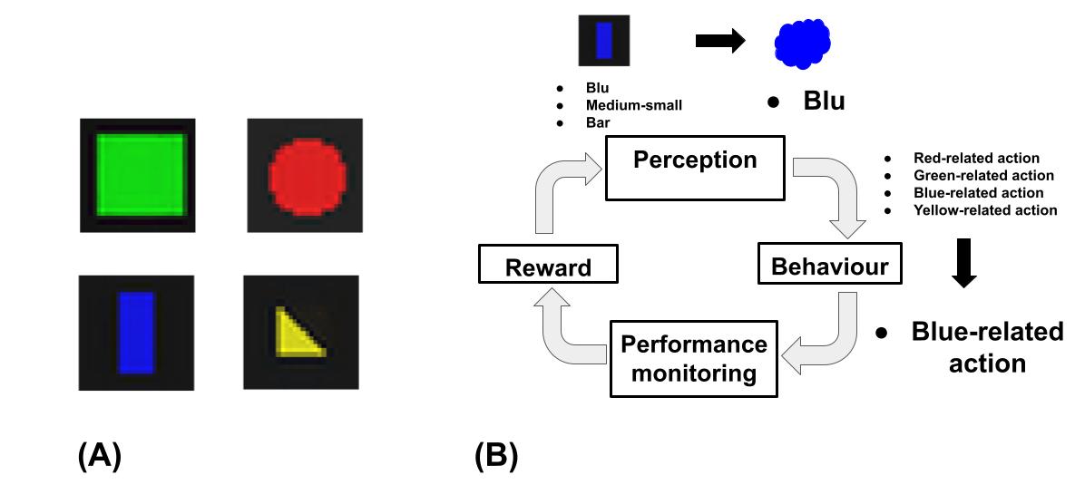
Figure 1: (A) Examples of the 64 geometrical shapes (circles, squares, parallelepipeds, triangles) used to produce the images. Each image encompasses a different attribute out of the four attributes of each of the three categories colour, shape, and size. (B) A schema of the main model processes involved in its interaction with the environment.

In particular, we focused on a sub-class of these tasks in which a classification rule is fixed and the participant has to execute a motor action on the basis of the features of a card (Hanania and Smith, 2010). The task uses a series of 2D input images of geometrical shapes varying in colour, shape, and size, for example as those shown in Figure 1A. For example in the case of a colour classification rule, the agent should learn to respond with a different output to the different colours (red, green, blue, yellow), hence ignoring the shape and the size. Figure 1B summarises the main processes performed by the system during the task performance: perception of the input, behavioural response, performance monitoring, and processing of the reward. The task was repeated for all the three classification rules involving colour, shape, and size.

2.2 The architecture of the model and its biological underpinning

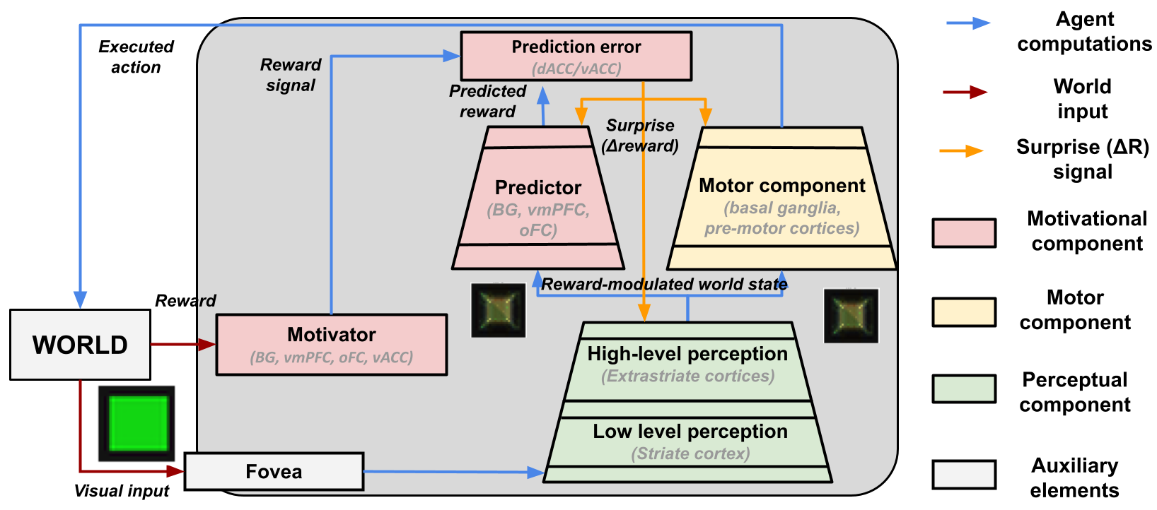
Figure 3: Schema of the model components and functions, the flows of information between the components, and the learning signals.

Figure 2 summarises at a high level the elements of the hypothesis proposed here that are captured by the computational model. This in particular encompasses intermediate layers corresponding to extra-striate cortices that host mixed UL and RL processes. Figure 3 shows the architecture of the model. We now illustrate the components of the architecture and their biological underpinning.

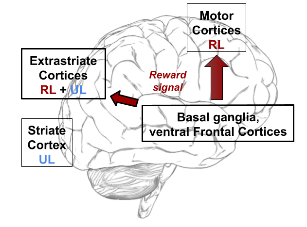
Figure 2: Scheme of learning processes and targeted brain areas that are addressed by the hypothesis and computational model presented here. The non-motor cortex undergoes both associative learning (UL) and trial-and-error learning (RL). The latter presents a gradient having a decreasing strength moving from the motor cortex towards the striate cortex. The model studies the effects that the mix of unsupervised and reinforcement-learning processes have in extrastriate cortices.

Perceptual component

This component is based on a neural network that processes visual inputs by performing information abstraction and mimics the brain visual cortical system. In particular, the component executes a hierarchical information processing (Felleman and Van Essen, 1991; Baldassarre et al., 2013) from the low-level retinotopic features in the striate cortex (V1), to the extraction of high-level image features (colour, shape, size) in the extrastriate cortices (DeYoe et al., 1996; Konen and Kastner, 2008).

Differently from the biologically implausible gradient-descent methods, the network learns through a bio-plausible mechanism (Illing et al., 2019). In particular, the learning processes used in the model update each connection weight (synapse) on the basis of locally available information related to the pre-synaptic and post-synaptic units. Another biologically plausible feature of the model, at the core of the novelty of the hypothesis presented here, is that the top layer of this component is trained during the task through a mechanism that integrates associative and reward-based RL (Figure 2).

The bottom layer of the component, which mimics early visual cortices, is instead trained before the task execution to reflect the learning of these areas during early development (Siu and Murphy, 2018). Critical for our hypothesis, this architecture captures the essence of the effects of dopamine reward signals onto extra-striate cortices and the lack of it in striate cortices (Williams and Goldman-Rakic, 1993; Jacob and Nienborg, 2018; Impieri et al., 2019; Niu et al., 2020; Froudist-Walsh et al., 2020). Finally, the model relies on distributed representations, for which information on each content (e.g., a percept) is encoded by many units of the layer, and each unit takes part in the representations of different contents. This encoding is more bio-plausible than localistic representations (‘grandmother-cells’; McClelland et al., 1986; Quiroga et al., 2008).

Motor component

This component is supported by a neural network that, on the basis of the perceptual component activation, produces an ‘action’ affecting the world. The network is trained through a trial-and-error learning algorithm using a reward signal, mimicking the interactions of basal ganglia with motor cortices during the learning of actions (Kim et al., 2017; Seger, 2008).

Motivational component

This component is formed by three sub-modules that emulate the motivational functions supported by different brain sub-systems.

First, a motivator sub-module produces a reward signal on the basis of the perceived outcome following action performance. Here the outcome is received from the environment and informs the system on the ‘correctness’ of the performed action (see below). This action-outcome might correspond to an ‘extrinsic reward’, for example to the receipt of food or other rewarding resources; this is suitably processed by the system sensors and motivator component to produce a reward signal guiding the system learning processes. In other conditions (Baldassarre and Mirolli, 2013; Baldassarre, 2011) the reward signal might be produced by intrinsic motivation processes, for example related to the novelty or surprise of the experienced stimuli (Barto et al., 2013) or to the acquisition of competence during the accomplishment of a desired goal (White, 1959; Santucci et al., 2016). In the brain, structures such as the hypothalamus and the pedunculopontine nucleus, and the ventromedial, orbital, and anterior-cingulate cortices, support extrinsic rewards (Panksepp, 1998; Mirolli et al., 2010), while other structures, such as the superior colliculus, hippocampus, and the dorsolateral prefrontal cortex, support the computation of intrinsic reward signals (Lisman and Grace, 2005; Ribas-Fernandes et al., 2011; Baldassarre, 2011).

Second, a predictor sub-module, based on a multi-layer neural network, uses the high-level perceptual representations encoding the current perceived state, received from the top layer of the perceptual component, to predict the rewards that can be attained from it. This module functionally mimics the brain basal-ganglia striosomes (Houk et al., 1995).

Last, a prediction error sub-module integrates the obtained and predicted rewards and produces a learning signal (‘surprise’). This signal influences the learning of the predictor, of the motor component and, most importantly, of the perceptual component. In the brain, this signal is represented by the phasic dopamine bursts reaching various target areas (Schultz, 2002), as also modelled by the actor-critic RL architecture (Barto, 1995).

2.3 Computational implementation and learning algorithms of the model

The system proposed here (Figure 4) is formed by a generative model integrated into an actor-critic architecture (Sutton et al., 1998), both modified to study the role of reward in perceptual representation learning. Further details regarding the system parameters (e.g., the number of units of each layer, the learning rates, the training epochs, etc.) are reported in Table S1 of the Supplementary Materials. The code of the system will be made publicly available online in GitHub in the case of publication.

Perceptual component

This component is a generative Deep Belief Network (DBN; Hinton et al., 2006; Le Roux and Bengio, 2008) composed of two stacked Restricted Boltzmann Machines (RBM; Hinton, 2012). Each RBM is composed of an input layer (‘visible layer’) and a second layer (‘hidden layer’) formed by Bernoulli-logistic stochastic units where each unit $j$ has an activation $h_{j}\in\{0,1\}$:

$$h_{j} =\begin{cases}1\ if\ \nu\geq\sigma(p_{j})\\ 0\ if\ \nu<\sigma(p_{j})\end{cases}$$ (1)

$$\sigma(p_{j}) =\frac{1}{1+e^{-p_{j}}}$$

$$p_{j} =\sum_{i}(w_{ji}\cdot v_{i})$$

where $\sigma(x)$ is the sigmoid function, $p_{j}$ is the activation potential of the unit $h_{j}$, $\nu$ is a random number uniformly drawn from $(0,1)$ for each unit, and $w_{ji}$ is the connection weight between the visible unit $v_{i}$ and $h_{j}$. The RBM is capable of reconstructing the input by following an inverse activation from the hidden layer to the input layer.

The DBN consists of a stack of RBMs—two in the model—where each RBM receives as input the activation of the hidden latent layer of the previous RBM. The model is trained layer-wise, starting from the RBM which receives inputs from the environment and towards the inner layers. On this basis, the DBN executes an incremental dimensionality reduction of the input, as higher layers further compress the representations received from the lower/previous RBM (Hinton and Salakhutdinov, 2006). In the model, the first RBM directly receives the input images and it is trained to encode them ‘offline’ before the task. This training uses the Contrastive Divergence, an unsupervised-learning algorithm that computes each connection weight update $\Delta\it{w_{ij}}$ as follows:

$$\Delta\it{w_{ij}}=\epsilon(\langle\it{v_{i}\cdot h_{j}}\rangle_{\it{data}}-\langle\it{v_{i}\cdot h_{j}}\rangle_{\it{model}})$$ (2)

where $\epsilon$ is the learning rate, $\langle\it{v_{i}\cdot h_{j}}\rangle_{\it{data}}$ is the product between the initial input (initial visible activation) and the consequent hidden activation averaged over all data points, $\langle\it{v_{i}\cdot h_{j}}\rangle_{\it{model}}$ is the product between the reconstructed visible activation and a second activation of the hidden layer following it averaged over all data points. The third and fourth activations are denoted with ‘model’ as they tend to more closely reflect the spontaneous input-independent activations of the RBM.

The second RBM of the model is trained ‘online’ during the task performance based on the novel algorithm proposed here. The algorithm integrates Contrastive Divergence (Eq. 2) with the REINFORCE algorithm described in the next session (Eq. 4) as follows:

$$\begin{split}\Delta\it{w_{ij}}=&\ \lambda\ (\epsilon\ (\langle\it{v_{i}\cdot h_{j}}\rangle_{\it{data}}-\langle\it{v_{i}\cdot h_{j}}\rangle_{\it{model}}))\ +\\ &\ (1-\lambda)\ (\alpha\ (r-\bar{r})(y_{\it{j}}-p_{\it{j}})x_{\it{i}})\end{split}$$ (3)

where $\lambda$ is the contribution of Contrastive Divergence to the update of weights, and $(1-\lambda)$ the contribution of REINFORCE. Crucial for this work, $\lambda$ mixes the contribution of UL and RL processes to the weight update, in particular a high value of it implies a dominance of UL whereas a low value of it implies a dominance of RL. In the simulations, we tested five values of the parameter: $\lambda\in\{1,0.1,0.01,0.001,0\}$.

Motor component

This component is a single-layer neural network trained with the RL algorithm REINFORCE (Williams, 1992). The input of the network is the activation of the last layer of the perceptual component. The network output layer is composed of Bernoulli-logistic units as for the perceptual component. The algorithm computes the update $\Delta\it{w_{ji}}$ of each connection weight linking the input unit $i$ and the output unit $j$ of the component as follows:

$$\Delta\it{w_{ji}}=\alpha(r-\bar{r})(y_{\it{j}}-\sigma(p_{\it{j}}))x_{\it{i}}$$ (4)

where $\alpha$ is the learning rate, $r$ is the reward signal received from the motivator, $\bar{r}$ is the reward signal expected by the predictor, $x_{\it{i}}$ is the input of the network (from the outer second hidden layer of the DBN), $\sigma(p_{\it{j}})$ is the sigmoidal activation potential of the unit encoding its probability of firing, and $y_{\it{j}}$ is the unit binary activation.

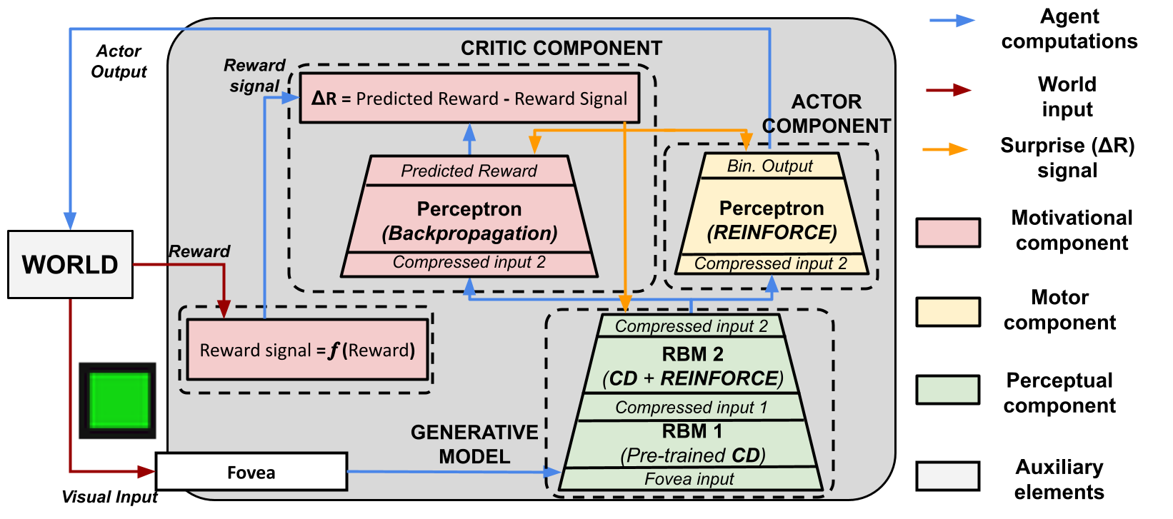
Figure 4: A computational schema of the model components and their training algorithms, the flows of information between the components, and the learning signals.

Motivational component

This component implements the functions of the critic component of an actor-critic architecture (Sutton et al., 1998) based on three sub-modules introduced in the previous section.

The motivator module computes the reward signal by scaling the reward perceived from the external environment into a standard value, the reward signal $r\in(0,1)$:

$$r=f(Reward)$$ (5)

where $Reward$ is the reward perceived from the environment and $f(.)$ is a linear scaling function ensuring that the reward signal ranges between $0$, corresponding to a wrong action, to $1$, corresponding to an optimal action. This reward signal represents the pivotal guidance of the RL processes driving the acquisition of not only the actions but also the DBN second hidden layer. As discussed above, in other cases the motivator might compute more complex reward signals based on more sophisticated types of extrinsic and/or intrinsic motivation mechanisms.

The predictor module is a multi-layer perceptron composed of an input layer (DBN second hidden layer), a hidden layer, and an output linear unit predicting the expected reward signal $\bar{r}$. The perceptron is trained with a standard gradient descendent method (McClelland et al., 1986; Amari, 1993) using a learning rate $\alpha$ and the error $e$ computed by the prediction-error component.

The prediction error module is a function that computes the reward prediction error (surprise) $e$ as follows:

$$e=r-\bar{r}$$ (6)

where $r$ is the reward signal from the motivator, and $\bar{r}$ is the expected reward signal produced by the evaluator. This error is used to train the predictor itself, the motor component, and the perceptual component.

Auxiliary elements

The input dataset is formed by RGB images with a black background and a polygon at the centre (Figure 1). The polygon is characterised by a unique combination of specific attributes chosen from three visual categories: colour, form and size. There are four attributes for each category: red, green, blue, yellow (colour); square, circle, triangle, bar (form); large, medium-large, medium-small, small (size). These attributes generate $4^{3}=64$ combinations forming the images used in the test.

The retina component is implemented as a $28\times 28\times 3$ matrix containing the RGB visual input. The matrix is unrolled into a vector of $2,352$ elements that represents the input of the perceptual component.

The environment is implemented as a function that provides an image to the model at each trial. In one trial the model perceives and processes one input image and undergoes a cycle of the aforementioned learning processes based on the reward received from the environment after the action performance. Here the environment computes the reward $r^{\prime}$ simply on the basis of the Euclidean distance between the model action and an ‘optimal action’:

$$Reward=\|\mathbf{y}^{*}-\mathbf{y}\|_{1}$$ (7)

where $\mathbf{y}^{*}$ is the optimal action binary vector that the model should produce for the current input, $\mathbf{y}$ is the model binary action, and $\|.\|_{1}$ is the L1 norm of the vectors difference. The optimal actions are four binary random vectors that the model should produce in correspondence to the items of the four input categories of the given task.

3 Results

We tested the model with different tasks each involving one out of three sorting rules based on the three categories, for example, a task required sorting the cards by colour and another one by shape. The model was tested with five different levels of UL/RL contribution ($\lambda$ parameter, see Section 2.3) and two levels of internal resources, in particular respectively $10$ and $50$ units in the second DBN hidden layer. Note that $50$ units were sufficient to allow the system to fully encode the image features, as shown by a preliminary test indicating a close-to-null reconstruction error.

We varied the parameters of these environmental and model conditions with a random grid search based on $1016$ simulations. The simulations were run in the Neuroscience Gateway platform (NSG, Sivagnanam et al., 2013). The different values of the critical parameter $\lambda$ gave rise to five conditions labelled as follows: Level 0 (L0): no RL (i.e., only UL); Level 1 (L1): low RL; Level 2 (L2): moderate RL; Level 3 (L3): high RL; Level 4 (L4): extreme RL (no UL). The simulations using different amounts of internal resources allowed us to investigate how the available computational resources affect the results related to the UL/RL mix.

The presentation of results is organised in three parts. The first part investigates the effects on the performance of the different contributions of UL/RL. The second part investigates the nature of the perceptual representations acquired through a different UL/RL learning mix. Finally, the third part presents a graphical reconstruction of the original input patterns produced by the generative perceptual component of the model and the related reconstruction errors.

Performances analysis

Figure 5 shows the training curves of the models trained with different RL contributions in 15,000 epochs. The L0 models, using only UL, learn faster during the first 1,000 epochs but exhibits the worst final performance. Figures S1, S2 and S3 in Supplementary Materials show that this effect is also present in subsets of all simulations. Instead, the highest final performance is achieved by the L3 models where UL and RL are better balanced.

Learning curves of models

Figure 5: Reward per epoch of the five models involving different UL/RL levels, averaged over the models using a given level. Shaded areas represent the curves standard deviations.

Figure 6 shows the final performance of the models, namely the maximum reward they achieved. A correlation analysis shows the presence of a linear relation between such performance and the level of the RL, but this is not very high thus indicating the relevance of the inverted U shape of the curve visible from the figure ($r=0.5$, $p<0.001$). A one-way ANOVA confirms the presence of a statistical difference between the final performance of the five groups ($F=47.51$, $p<0.001$).

Performance of models

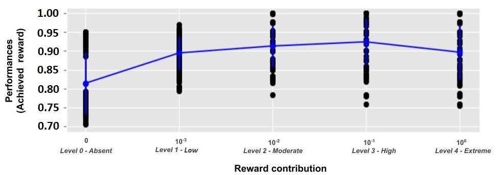
Figure 6: Performances (maximum reward obtained at the end of training) of models featuring different levels of RL contribution.

Post hoc tests (Table 1) confirm that the performances of models with an absent RL contribution (L0) are statistically different with respect to each of the other models ($0.81\pm 0.08$, $p<0.001$). The L3 models show a higher performance compared to the L0 models ($0.92\pm 0.06$ vs. $0.81\pm 0.08$, $p<0.001$), the L1 models ($0.92\pm 0.06$ vs. $0.89\pm 0.04$, $p<0.001$), and the L4 models ($0.92\pm 0.06$ vs. $0.90\pm 0.07$, $p<0.05$). The L2 and L3 models do not show a significant difference ($0.92\pm 0.06$ vs. $0.91\pm 0.05$).

	Absent (L0)	Low (L1)	Moderate (L2)	High (L3)	Extreme (L4)
Absent (L0)	//	//	//	//	//
Low (L1)	$p<0.001$	//	//	//	//
Moderate (L2)	$p<0.001$	$p>0.05$ (NS)	//	//	//
High (L3)	$p<0.001$	$p<0.001$	$p>0.05$ (NS)	//	//
Extreme (L4)	$p<0.001$	$p>0.05$ (NS)	$p>0.05$ (NS)	$p<0.05$	//

Table 1: Post-hoc comparisons (t-test with Bonferroni correction) between the performance of models with different levels of RL contribution. ‘NS’ indicates ‘non statistically significant’.

To further investigate the relationship between the performance of the models and the different levels of RL contribution, we grouped the results of the simulations on the basis of the computational resources or the sorting rule. Here we present a summary of the results while Section S2.1 in the Supplemental Materials reports the posthoc tests.

Table 2 shows that the increase of computational resources available for the representations tends to lower the amount of RL contribution leading to the highest performance. Indeed, a one-way ANOVA shows a statistical difference between the models ($F=3.85$, $p<0.001$) and the post-hoc tests show that the L2 model leads to the best result ($0.95\pm 0.05$).

The table also highlights differences between the simulations using different sorting rules (colour, shape, size). The simulations with the colour sorting rule show flattened reward values with respect to the different RL contribution. In the case of low computational resources the model does not show statistically significant differences ($F=0.88$, $p>0.05$). A difference emerges in the case of high computational resources ($F=19.8$, $p<0.001$) where the L2 models, having a balanced UL/RL mix, show the best final performance ($0.98\pm 0.02$).

The simulations with the shape sorting rule show statistical differences with both low computational resources ($F=120.9$, $p<0.001$) and high computational resources ($F=20.4$, $p<0.001$). In both cases, the models using a mixed level of UL and RL prevail: the extreme cases of the L0 models (only UL), and L4 models (only RL) have lower performances with respect to the L1, L2 and L3 models having a more balanced UL/RL mix.

Finally, the simulations with the size sorting rule show statistical differences with low computational resources ($F=43.4$, $p<0.001$) but not with ‘high computational resources’ ($F=1.12$, $p>0.05$). In the first case, the L0 models have the lowest performance.

	Absent	Low	Moderate	High	Extreme
Low Resources	$0.81\pm 0.08$	$0.89\pm 0.04$	$0.91\pm 0.05$	$\mathbf{0.92}\pm 0.06$	$0.90\pm 0.07$
Colour	$0.92\pm 0.02$	$\mathbf{0.92}\pm 0.02$	$0.91\pm 0.04$	$0.91\pm 0.07$	$0.90\pm 0.08$
Shape	$0.75\pm 0.02$	$0.89\pm 0.04$	$0.94\pm 0.04$	$\mathbf{0.95}\pm 0.04$	$0.93\pm 0.06$
Size	$0.76\pm 0.02$	$0.88\pm 0.05$	$0.89\pm 0.06$	$\mathbf{0.90}\pm 0.06$	$0.86\pm 0.07$
High Resources	$0.92\pm 0.03$	$0.93\pm 0.04$	$\mathbf{0.95}\pm 0.05$	$0.93\pm 0.06$	$0.93\pm 0.05$
Colour	$0.94\pm 0.01$	$0.94\pm 0.01$	$\mathbf{0.98}\pm 0.02$	$0.95\pm 0.03$	$0.96\pm 0.02$
Shape	$0.93\pm 0.02$	$0.97\pm 0.02$	$\mathbf{0.97}\pm 0.02$	$0.96\pm 0.02$	$0.94\pm 0.02$
Size	$0.88\pm 0.02$	$0.88\pm 0.03$	$\mathbf{0.90}\pm 0.05$	$0.88\pm 0.07$	$0.88\pm 0.07$

Table 2: Performance of models with different RL contributions in correspondence to two different amounts of computational resources (number of neurons in the second hidden layer of the DBN) and three different sorting rules (colour, shape, size). Figures in bold highlight the highest value per each condition (along the raws).

Analysis of internal representations

To investigate the nature of the perceptual representations acquired by the models, we show the results of some example simulations in the cases of different sorting rules and different levels of the RL. Other simulations lead to qualitatively similar results.

To visualise the representations we used a Principal Component Analysis (PCA), allowing a dimensionality reduction, and a K-means algorithm, supporting clustering. In particular, we extracted the first two principal components of the input patterns reconstructed by the model into the visible layer in correspondence to the original 64 input patterns. The reconstructed images were obtained by spreading the activity from the visible layer of the DBN, activated with an image, to its first and second hidden layer, and then back towards the visible layer. We analysed the reconstructed visual representations, rather than the hidden representations, to assess which features of the original visual images are retained by the internal representations. The results of the PCA extraction of the two dimensions of the representations can be plotted in a 2D scatter plot to visualise the results of the following K-means algorithm. The K-means algorithm was applied to PCA 2D codes of the internal representations. We set $K=4$, so the algorithm grouped the representations into four classes, as the number of the actions. This made it possible to analyse how the model internally represents the different input images. Further details and results regarding these methods, as the cumulative variance explained by the PCA components and the silhouette scores of the K-mean algorithm, are reported in Section S2.2 of Supplemental Materials.

Colour sorting category: reconstructed input

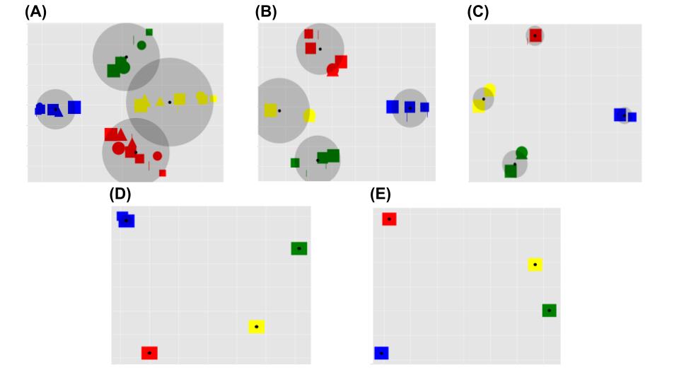
Figure 7: Principal components of the reconstructed image representations in the case of the colour sorting rule and in correspondence to different levels of RL (shown in different graphs). The dimensionality of the reconstructed image was reduced to two through a PCA (x-axis: first component; y-axis: second component). Within each graph, each reconstructed image is represented by a point marked by an icon that summarises the colour, shape, and size of the shape in the image (some icons are not visible as they overlap). The centroids of the four clusters found by the K-means algorithm are marked with a black dot, while the maximum distance of the points of the cluster from its centroid is shown by a grey circle. A: Level 0 (L0), absent RL (only UL); B: Level 1 (L1), low RL; C: Level 2 (L2), moderate RL; D: Level 3 (L3), high RL; E: Level 4 (L4), extreme RL (no UL).

Shape sorting category: reconstructed input

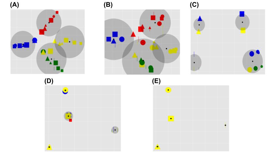
Figure 8: Principal components of the reconstructed image representations in the case of the shape sorting rule and in correspondence to different levels of RL. The plots are drawn as in Figure 7.

Size sorting category: reconstructed input

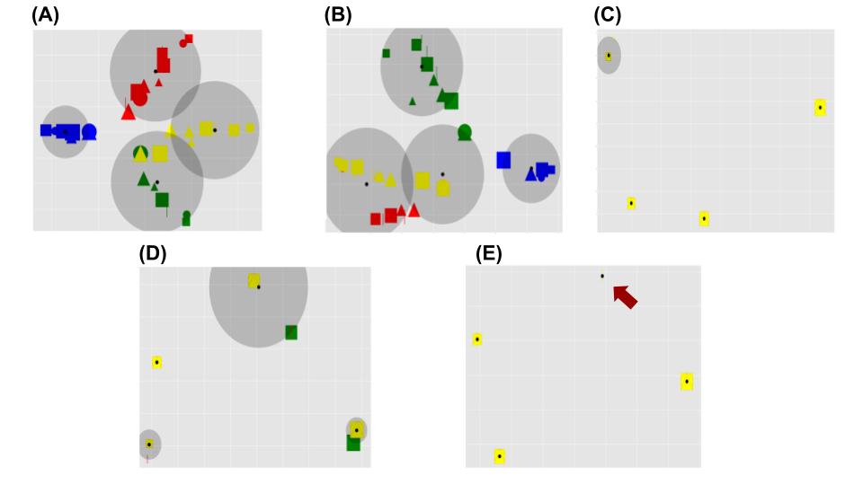
Figure 9: Principal components of the reconstructed image representations in the case of the size sorting rule and in correspondence to different levels of RL. The graphs are drawn as in Figure 7. The red arrow in graph E indicates the centroid of a cluster that contains only the small bars but not the other small shapes.

The results of the analyses (Figures 7-9) highlight that the reward-based RL contribution strongly affects the internal representations as revealed by the reconstructed inputs. For each sorting rule considered, models with a medium (L2) and high (L3) level of RL show the emergence of category-based clusters, with their radius progressively diminishing with an increasing weight of the RL. Conversely, the L0 and L1 models do not show this effect in any task condition. The only exceptions to this are the models with an absent or low RL (L0 and L1) showing a clustering effect that does not depend on the task but only on the colour of the shapes. This is due to the high distinctiveness of colours, largely activating different portions of the input units with respect to the other image features.

Figure 9-E shows that the model with an extreme RL incurred a clustering error. In particular, in this condition the model should group the images into four clusters (as in the conditions of Figure 9-C,D) whereas it tends to use only three clusters.

Information stored by the model

To further investigate what type of information is stored by the model, we show the results of two additional analyses. The first analysis examined the DBN reconstruction error (see Section S2.3 in Supplementary Materials for further details), while the second analysis qualitatively inspected the reconstructions of the input images.

Information loss for different levels of RL

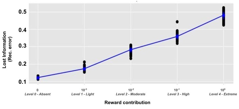
Figure 10: Information loss (reconstruction error at the end of the training) of models with different levels of RL.

Figure 10 shows the results of the first analysis and highlights the presence of a strong positive linear relationship between the level of RL and the reconstruction error ($r=0.68$, $p<0.001$). A one-way ANOVA confirmed the presence of a statistical difference between the five groups ($F>100.0$, $p<0.001$). These results indicate that an increasing RL contribution causes a progressive loss of information on the input images.

The results of the second analysis show the kind of information that the internal representations tend to retain, in particular if the system tends to store task-independent and/or task-related features. In this respect, Figure 11 highlights the emergence of shapeless coloured blobs in the case of the colour sorting rule, the emergence of colourless and sizeless prototypical shapes in case of shape sorting rule, and the emergence of colourless blobs with different sizes in the case of the size sorting rule.

Input reconstructions (sorting category: colour)

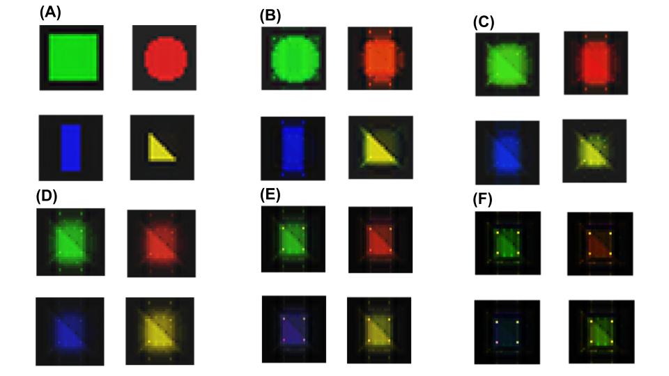
Input reconstructions (sorting category: shape)

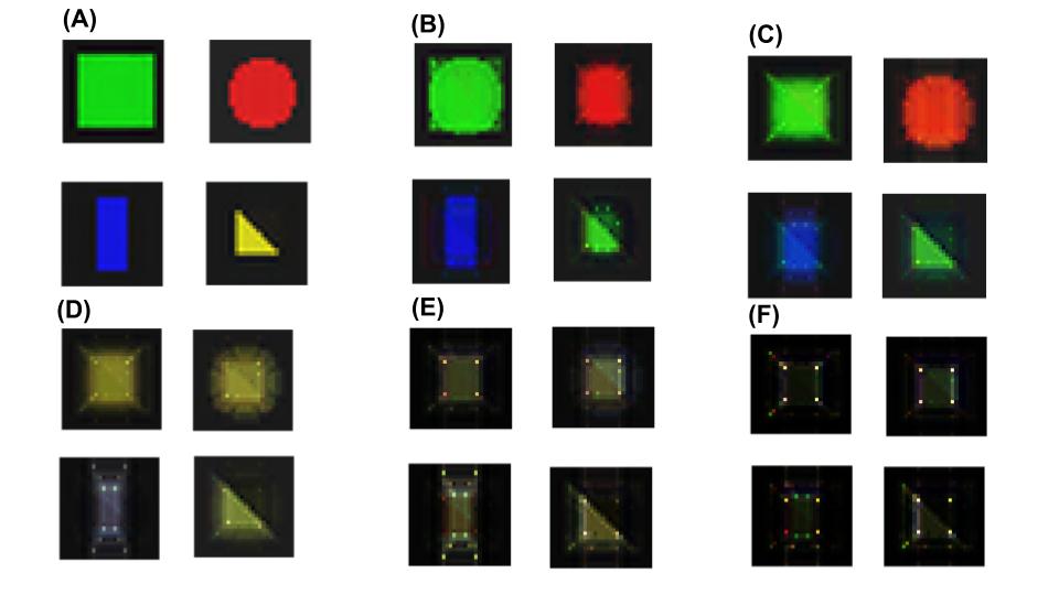
Input reconstructions (sorting category: size)

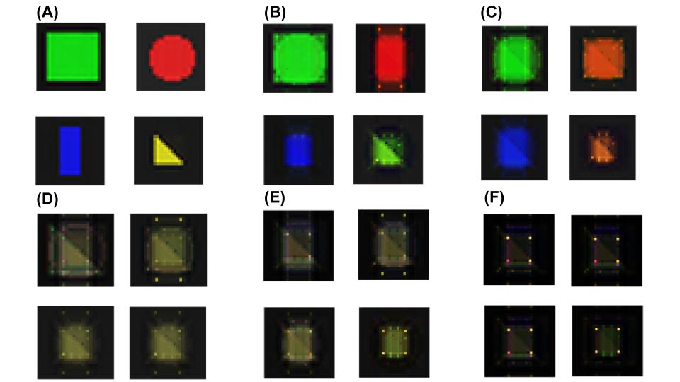
Figure 11: Image reconstructions with different sorting rules and different levels of RL. A: Original inputs; B: Level 0 (L0) - absent RL (only UL); C: Level 1 (L1) - low RL; D: Level 2 (L2) - moderate RL; E: Level 3 (L3) - high RL; F: Level 4 (L4) - extreme RL (only RL).

4 Discussion

In this work, we propose a novel hypothesis on the broad nature of learning in the brain cortex. A previous seminal view proposed that the cortex, basal ganglia, and cerebellum use the different learning mechanisms studied in machine learning, respectively unsupervised, reinforcement, and supervised learning (Doya, 1999, 2000). Recently, we have proposed a theory (Caligiore et al., 2019) that expands such view by proposing that, although those learning processes might be predominant in the three macro brain systems, plasticity within them mixes the three learning mechanisms. The hypothesis proposed here focuses on the cortex and on the empirical evidence showing that dopamine reaches cortical targets (Williams and Goldman-Rakic, 1993; Niu et al., 2020). On this basis, the hypothesis proposes that dopamine directly conveys information on the reward to the target cortices. Therefore, learning processes happening within them integrate associative (UL) and reward-based trial-and-error mechanisms (RL). Here we also present a computational model that actually mixes the two learning processes. The key idea at the core of the model is to exploit the stochastic nature of the units of Boltzmann neural networks to implement the RL key noise-based search process through the REINFORCE algorithm (Williams, 1992). The author of this algorithm envisaged the link between the stochastic units used in Boltzmann neural networks and those used in REINFORCE (Williams, 1992). However, the original work proposed the algorithm only to support the acquisition of actions as usually done in RL (Sutton et al., 2000, 1998). Instead, the model proposed here uses REINFORCE to learn inner representations in the neural network. This differs from other neural network models where reward only informs the training at the output layer of the network whereas the deeper representations are updated based on biologically non-plausible error back-propagation mechanisms (Arulkumaran et al., 2017; Mnih et al., 2015). To our knowledge, the proposed model is the first to allow reward signals to directly bias the acquisition of the representations encoded in the inner neural layers of the network in a bio-plausible manner. The model thus represents a new tool to investigate the potential utility of this for computational purposes and also to study the possible effects of the mixed UL/RL processes within the brain cortex.

The model was tested with a task having the features of experiments used in the field of category learning, in particular requiring sorting images based on different attributes of a given category (Hanania and Smith, 2010). This was done to start to consider how the model could be used to study specific phenomena in category learning (Zeithamova et al., 2019), as further discussed below.

The main result of the tests of the model is that a suitably balanced mix of UL and RL leads the model to achieve the best performance. This result holds for all tested conditions, as shown in Figure 6 and Table 1. Further analyses explained the possible causes of this.

The case of absent or low RL has some initial advantages at the beginning of training. This can be seen from Figure 5 where the pure UL case exhibits the learning curve with the sharpest initial increase of performance. Figures S1, S2 and S3 in Supplementary Materials show that this effect is also robustly present in sub-groups of simulations. The reason for this is that initially the models with high RL produce a highly variable exploratory behaviour, and thus the resulting reward signals that guide the learning process involving the deeper layers of the network are rare and unreliable. Instead, since the initial phases of training the UL process can proceed independently of the success of behaviour, and so it can build representations needed to support the learning of behaviour itself. However, with the advancement of training the conditions with absent/low levels of RL achieve a lower performance than the more balanced conditions, as shown in Figure 6 and Table 1. Figures S1, S2 and S3 in Supplementary Materials confirm the generality of this result. The reason is that UL tends to encode all features of the images, and so the task-relevant features compete with them and remain with insufficient computational resources.

This interpretation is corroborated by the tests where we manipulated the computational resources that were available to the system, and specifically the number of the reward-biased units at the second layer of the DBN (Table 2). These tests show that with a higher amount of computational resources the best performance is achieved by the models having a better balance of UL and RL, in particular a higher level of UL. This is because the encoding of task-irrelevant features is less impairing for the encoding of task-relevant features. To appreciate the relevance of this result, it should be considered that in ecological conditions the information received from sensors (e.g., the information from the retina) always overwhelms the available computational resources, and so some task-based feature selection is always advantageous.

At the opposite side of the spectrum, also models where RL is predominant or exclusive have computational limitations, as shown in Figure 6 and Table 1. The acquisition of internal representations is slow in models solely based on RL plasticity as learning is guided only by reward. Hence, the reconfiguration of the synaptic strengths are initially attained in an erratic fashion, as also discussed above (Figure 5). Importantly, the system tends to incur in local minima with the progression of learning, as shown in Figure 9E.

These results suggest the general possibility that UL and RL might express advantages at different stages of learning, in particular, UL might be more useful at the beginning of learning while RL at later stages. Future work might thus aim to study how to dynamically regulate the UL/RL balance during learning.

The generative nature of the perceptual component of the model allowed the investigation of how the internal representations tend to cluster the images depending on the categorisation rule of the task and the UL/RL mix balance. Graphs ‘A-B’ of Figures 7, 8, and 9 show that when RL is absent or low, UL tends to lead to the acquisition of all features of the image independently of their relevance for the task, as also shown by the low reconstruction error obtained in this cases (Figure 10). Instead, graphs ‘C, D’ of the same figures show how a mix of the two learning processes leads to the encoding of different attributes of the visual shapes. The images are grouped in relation to the responses to be associated to them, thus facilitating downstream action selection. Finally, when learning is only driven by reward, as shown by the graphs ‘E’ of the figures, the internal representations collapse to only one representation per group of images requiring a given action. This interpretation is also supported by the higher levels of the reconstruction error obtained in these cases (Figure 10).

Figure 11 exploits the generativity of the model to highlight the features of the images that RL tends to isolate when it is increasingly strong. As the figure shows, these are few features that strongly differentiate the shapes into the desired categories, for example features related to specific colours, or specific elements of the shapes or size. These representations favour learning of the downstream actions but imply less robustness and make the system vulnerable to local minima, as we have seen above. Moreover, this is expected to create representations that generalise poorly to new tasks, an important issue that deserves further investigation as it might justify why the brain seems to rely less on reward in early visual processing stages.

These results show how the presented model has the potential to be used to interpret the empirical experiments investigating the well-known phenomenon for which the tasks accomplished tend to modulate the acquired perceptual representations. This phenomenon has been shown in mice (Poort et al., 2015), primates (Sigala and Logothetis, 2002; De Baene et al., 2008; Emadi and Esteky, 2014), and also humans (de Beeck et al., 2006; Astafiev et al., 2004). In particular, the studies on humans involve the wide research field of ‘category learning’ (for reviews, see Ashby and Maddox 2011b; Zeithamova et al. 2019). The bulk of the research in this field has traditionally focused on the contrast between explicit versus procedural mechanisms for category learning (Maddox and Ashby, 2004; Seger and Miller, 2010) and more recently on the prototype versus example-based nature of the acquired sensory representations (Mack et al., 2013; Bowman and Zeithamova, 2018; Zeithamova et al., 2019). Although reward and RL are considered important for category learning (Seger and Peterson, 2013; Chelazzi et al., 2013), only recently few works have started to investigate how reward affects the acquired representations, the issue relevant for the hypothesis and model proposed here. For example, it has been shown that category learning in the ventromedial prefrontal cortex, inferior parietal cortex, and intraparietal sulcus are affected by the reward (Braunlich and Seger, 2016; Zeithamova et al., 2019). To our knowledge, however, we still do not know how reward might influence the formation of low-level representations of category features, for example within the extrastriate cortex of the brain parietal areas.

A final remark is that the proposed model is coherent with the theoretical framework of embodied perception (DiFerdinando and Parisi, 2004; Vernon, 2008; Foglia and Wilson, 2013) proposing that the brain constructs internal representations of the world “for being ready to act”. In this respect, the model specifies a possible ways in which the brain, based on the reward signals directly reaching its inner areas, might ‘warp’ representations in favour of the pursued tasks.

5 Conclusions

We have proposed the hypothesis that also non-motor cortices, in particular the extra-striate cortices, learn through both associative mechanisms (unsupervised learning) and reward-based mechanisms (reinforcement learning). Moreover, we have proposed a bio-plausible computational model facing a category-based sorting task to start to study how these mixed learning processes might affect the acquired representations of stimuli.

The results obtained with the tests of the model show that a suitably balanced mix of unsupervised and reinforcement learning processes leads to the highest performance. On one hand, excessive unsupervised learning tends to use computational resources to represent all input features and thus to leave scarce resources for the representation of task-relevant features. On the other hand, an excessive RL tends to lead to initial slow learning and to incur in local minima. Moreover, the results show how reward might lead to the acquisition of action-oriented representations on the basis of bio-plausible mechanisms, and this favours the selection of downstream actions.

In future work, the model could be used to address specific data on the reward-based modulation of category learning in the brain cortex. Moreover, the model prompts further computational studies directed to investigate the possible advantages of reward signals directly reaching the deep layers of artificial neural networks.

6 Acknowledgements

We thank the Neuroscience Gateway (Sivagnanam et al., 2013) used to run most of the simulations. This work has received funding from the European Union’s Horizon 2020 Research and Innovation Program, under Grant Agreement No 713010 of the project ‘GOAL-Robots – Goal-based Open-ended Autonomous Learning Robots’, and under Grant No 796135 of the H2020-MSCA-IF-2017 project ‘INTENSS’.

Supplementary Material

Methods: further details on the model simulations

We tested the model solving the sorting task with different task conditions (sorting rule, i.e. colour, shape or size) and perceptual component configurations (the number of neurons of top hidden layer and the reward contribution into the learning process). We randomly changed these parameters, keeping the others fixed. Table S1 shows the key parameters of simulations.

Simulations parameters

Label	Value/Range	Description
Sorting rule	$\{colour,shape,size\}$	Variable. latent rule to solve the sorting task
Training epochs	$15*10\textsuperscript{3}$	Fixed. Training epochs of sorting task.
Single-layer perceptron output units	$10$	Fixed. Output neurons of motor component.
Single-layer perceptron learning rate (REINFORCE)	$1*10\textsuperscript{-2}$	Fixed. Training learning rate of motor component.
Multi-layers perceptron hidden units	$50$	Fixed. Hidden neurons of predictor component.
Multi-layers perceptron learning rate (Backpropagation)	$1*10\textsuperscript{-3}$	Fixed. Training learning rate of predictor component.
Single-layer perceptron learning rate (REINFORCE)	$1*10\textsuperscript{-2}$	Fixed. Training learning rate of motor component.
DBN units (visible layer)	$2352$	Fixed. Neurons of visible layer.
DBN units (first hidden layer)	$200$	Fixed. Neurons of first hidden layer.
DBN units (second hidden layer)	$\{10,50\}$	Variable. Neurons of second hidden layer.
First RBM (off-line) training epochs	$1*10\textsuperscript{3}$	Fixed. Training epochs necessary to achieve a dataset reconstruction error of $0.001$.
First RBM learning rate (Constrastive Divergence)	$1*10\textsuperscript{-2}$	Fixed. Training (offline) learning rate.
First RBM momentum (Constrastive Divergence)	$0.9$	Fixed. Training (offline) momentum.
Second RBM learning rate (Constrastive Divergence)	$1*10\textsuperscript{-3}$	Fixed. Training learning rate.
Second RBM momentum (Constrastive Divergence)	$0.9$	Fixed. Training momentum.
Second RBM learning rate (REINFORCE)	$1*10\textsuperscript{-2}$	Fixed. Training learning rate.
$\lambda$	$\{1,0.1,0.01,0.001,0\}$	Variable. Contribution of the Contrastive Divergence to the weights update
Second RBM reward contribution	$(1-\lambda)$, with $\lambda\in\{1,0.1,0.01,0.001,0\}$	Variable. Contribution of the REINFORCE to the weights update

Table S1: The table shows the simulations parameters.

Results: further statistical analysis

Performances analysis

Figures S1, S2, and S3 show the training curves of the models trained with different RL contributions in 15,000 epochs, for the three sorting categories and for the condition with 10 units of the DBN second hidden layer. Figures S4, S5, and S6 show the analogous curves for the condition involving 50 units of the DBN second hidden layer. In particular, these are the models of the condition with a high-level of computational resources, namely 50 units at the level of the second hidden layer of the DBN. In all conditions, the L0 models (with no reinforcement learning - RL, i.e. relying only on unsupervised learning - UL) show an initial highest performance with respect to the other models L1, L2, L3, and L4. This confirms that in L0 models representation learning is initially facilitated with respect to models with a higher RL contribution as the reward is initially erratic. Moreover, for all three category tasks the reward achieves a maximum final performance for the L2 models having a balanced level of UL and RL. Indeed, these models outperform the models with absent or very low RL (L0 and L1) because these employ a lot of computational resources for non-task specific features; moreover they outperform the models with very high or extreme RL (L3 and L4) because these tend to incur in local minima.

Learning curves of models: colour category, low computational resources

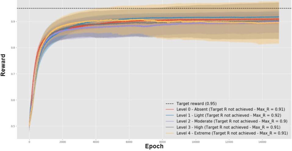
Figure S1: Reward per epoch in the task task involving the colour category and low computational resources, of the five models involving different UL/RL levels, averaged over the models using a given level. Shaded areas represent the curves standard deviations.

Learning curves of models: shape category, low computational resources

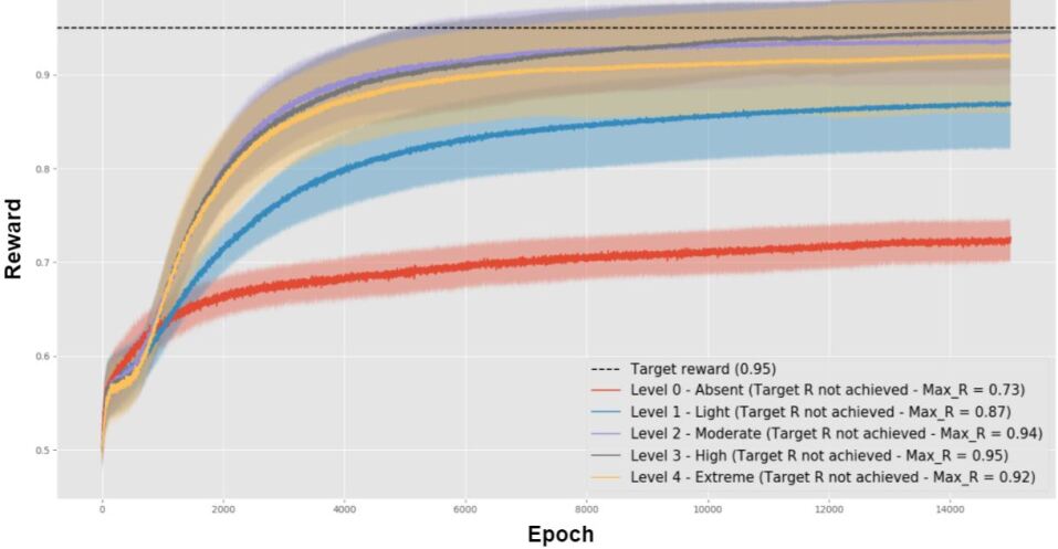
Figure S2: Reward per epoch in the task task involving the shape category and low computational resources, of the five models involving different UL/RL levels, averaged over the models using a given level. Shaded areas represent the curves standard deviations.

Learning curves of models: size category, low computational resources

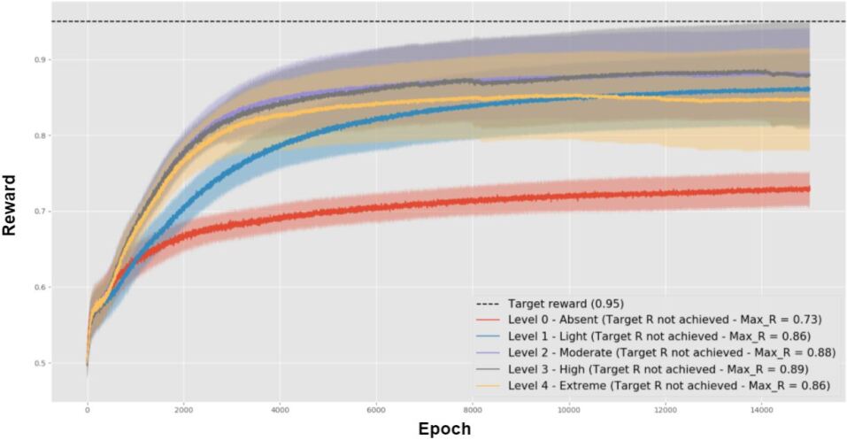
Figure S3: Reward per epoch in the task task involving the size category and low computational resources, of the five models involving different UL/RL levels, averaged over the models using a given level. Shaded areas represent the curves standard deviations.

Learning curves of models: colour category, high computational resources

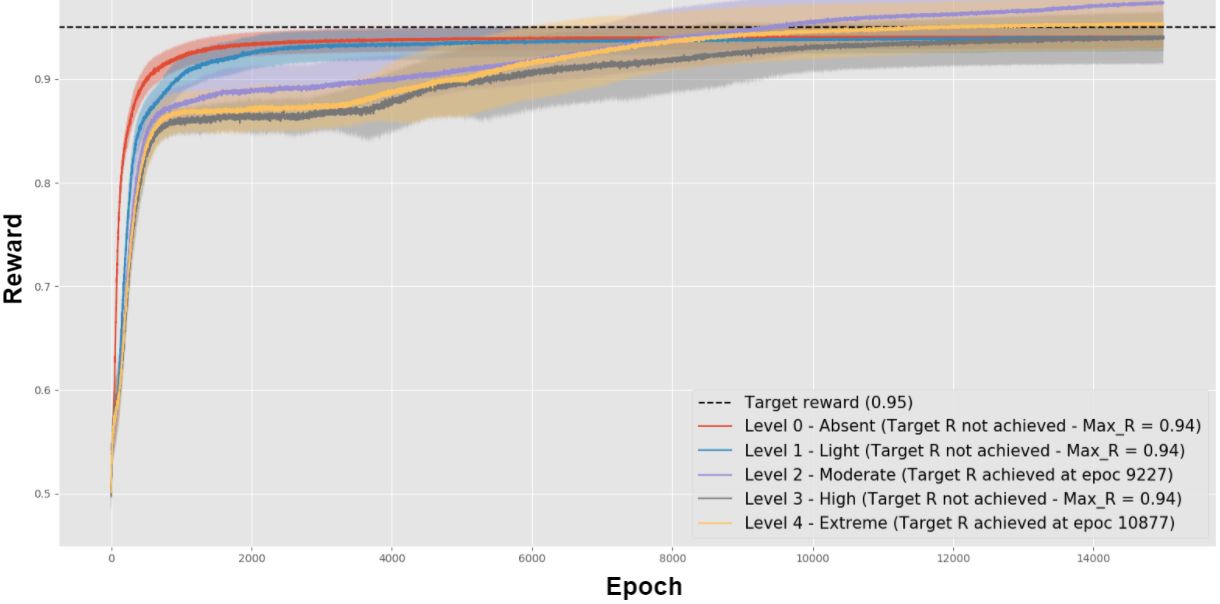
Figure S4: Reward per epoch in the task task involving the colour category and high computational resources, of the five models involving different UL/RL levels, averaged over the models using a given level. Shaded areas represent the curves standard deviations.

Learning curves of models: shape category, high computational resources

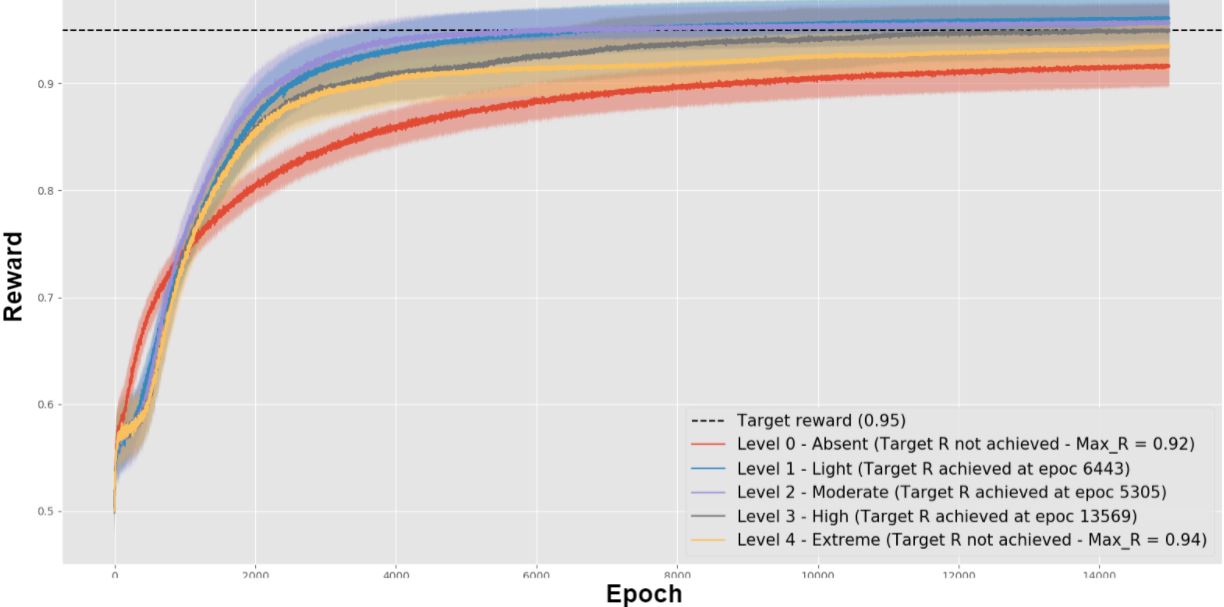
Figure S5: Reward per epoch in the task task involving the shape category and high computational resources, of the five models involving different UL/RL levels, averaged over the models using a given level. Shaded areas represent the curves standard deviations.

Learning curves of models: size category, high computational resources

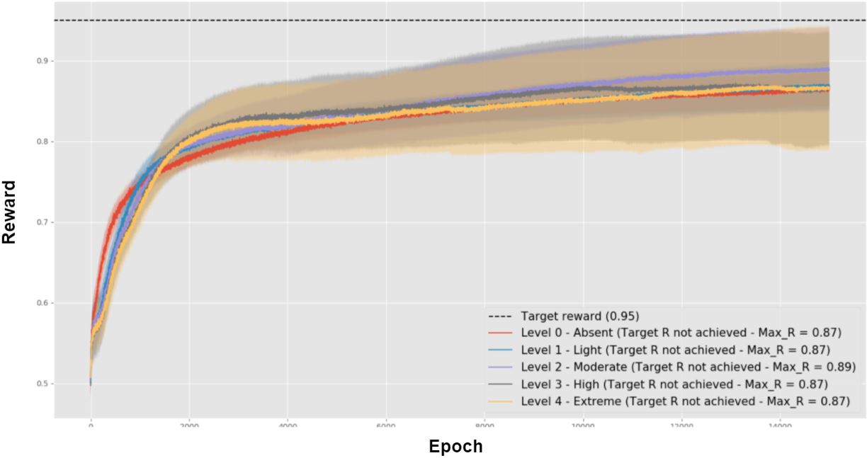
Figure S6: Reward per epoch in the task task involving the size category and high computational resources, of the five models involving different UL/RL levels, averaged over the models using a given level. Shaded areas represent the curves standard deviations.

Table S2 shows the post-hoc tests with the Bonferroni correction. The tests are grouped for each specific combination of the three main conditions, that is, computational resources (2 conditions), sorting rule used in the task (3 conditions), and reward contribution (5 conditions).

Sorting rule: Colour, Computational Resources: Low

	Absent (L0, N = $40$)	Low (L1, N = $34$)	Moderate (L2, N = $21$)	High (L3, N = $38$)	Extreme (L4, N = $32$)
Absent (L0)	//	$p>0.05$ (NS)	$p>0.05$ (NS)	$p>0.05$ (NS)	$p>0.05$ (NS)
Low (L1)	//	//	$p>0.05$ (NS)	$p>0.05$ (NS)	$p>0.05$ (NS)
Moderate (L2)	//	//	//	$p>0.05$ (NS)	$p>0.05$ (NS)
High (L3)	//	//	//	//	$p>0.05$ (NS)
Extreme (L4)	//	//	//	//	//

Table S2: The table shows the post hoc multiple comparisons (t-test with Bonferroni correction) of models in case of the colour sorting rule and low computational resources. NS = not significant.

Sorting rule: Shape, Computational Resources: Low

	Absent (L0, N = $32$)	Low (L1, N = $44$)	Moderate (L2, N = $29$)	High (L3, N = $42$)	Extreme (L4, N = $39$)
Absent (L0)	//	$p<0.001$	$p<0.001$	$p<0.001$	$p<0.001$
Low (L1)	//	//	$p<0.001$	$p<0.001$	$p<0.01$
Moderate (L2)	//	//	//	$p>0.05$ (NS)	$p>0.05$ (NS)
High (L3)	//	//	//	//	$p>0.05$ (NS)
Extreme (L4)	//	//	//	//	//

Table S3: The table shows the post hoc multiple comparisons (t-test with Bonferroni correction) of models in case of the shape sorting rule and low computational resources. NS = not significant.

Sorting rule: Size, Computational Resources: Low

	Absent (L0, N = $38$)	Low (L1, N = $35$)	Moderate (L2, N = $39$)	High (L3, N = $28$)	Extreme (L4, N = $41$)
Absent (L0)	//	$p<0.001$	$p<0.001$	$p<0.001$	$p<0.001$
Low (L1)	//	//	$p>0.05$ (NS)	$p>0.05$ (NS)	$p>0.05$ (NS)
Moderate (L2)	//	//	//	$p>0.05$ (NS)	$p>0.05$ (NS)
High (L3)	//	//	//	//	$p>0.05$ (NS)
Extreme (L4)	//	//	//	//	//

Table S4: The table shows the post hoc multiple comparisons (t-test with Bonferroni correction) of models in case of the size sorting rule and low computational resources. NS = not significant.

Sorting rule: Colour, Computational Resources: High

	Absent (L0, N = $39$)	Low (L1, N = $33$)	Moderate (L2, N = $31$)	High (L3, N = $20$)	Extreme (L4, N = $43$)
Absent (L0)	//	$p>0.05$ (NS)	$p<0.001$	$p>0.05$ (NS)	$p<0.01$
Low (L1)	//	//	$p<0.001$	$p>0.05$ (NS)	$p<0.05$
Moderate (L2)	//	//	//	$p<0.001$	$p<0.01$
High (L3)	//	//	//	//	$p>0.05$ (NS)
Extreme (L4)	//	//	//	//	//

Table S5: The table shows the post hoc multiple comparisons (t-test with Bonferroni correction) of models in case of the colour sorting rule and high computational resources. NS = not significant.

Sorting rule: Shape, Computational Resources: High

	Absent (L0, N = $41$)	Low (L1, N = $35$)	Moderate (L2, N = $33$)	High (L3, N = $29$)	Extreme (L4, N = $33$)
Absent (L0)	//	$p<0.001$	$p<0.001$	$p<0.001$	$p>0.05$ (NS)
Low (L1)	//	//	$p>0.05$ (NS)	$p>0.05$ (NS)	$p<0.001$
Moderate (L2)	//	//	//	$p>0.05$ (NS)	$p<0.001$
High (L3)	//	//	//	//	$p<0.05$
Extreme (L4)	//	//	//	//	//

Table S6: The table shows the post hoc multiple comparisons (t-test with Bonferroni correction) of models in case of the shape sorting rule and high computational resources. NS = not significant.

Sorting rule: Size, Computational Resources: High

	Absent (L0, N = $24$)	Low (L1, N = $30$)	Moderate (L2, N = $35$)	High (L3, N = $29$)	Extreme (L4, N = $29$)
Absent (L0)	//	$p>0.05$ (NS)	$p>0.05$ (NS)	$p>0.05$ (NS)	$p>0.05$ (NS)
Low (L1)	//	//	$p>0.05$ (NS)	$p>0.05$ (NS)	$p>0.05$ (NS)
Moderate (L2)	//	//	//	$p>0.05$ (NS)	$p>0.05$ (NS)
High (L3)	//	//	//	//	$p>0.05$ (NS)
Extreme (L4)	//	//	//	//	//

Table S7: The table shows the post hoc multiple comparisons (t-test with Bonferroni correction) of models in case of the size sorting rule and high computational resources. NS = not significant.

Reconstruction error and information stored

In this section we explain why the reconstruction errors of the DBN reported in the main text can be considered a measure of the information on the input patterns retained by this component of the models. Restricted Boltzmann Machines and Deep Belief Networks are generative models able to store the joint probability between an input and the consequent hidden layer activation (Hinton et al., 2006; Hinton, 2012). This property makes these models able to execute a dimensional reduction of input patterns (Hinton and Salakhutdinov, 2006) and to ‘generate’ such input patters based on an inverse spread of activation spread from a hidden layer towards the visible layer. Due to the difficulty of meaningfully activating the distributed representations within the hidden layers in a direct way, a typical way to exploit this generativity property also followed here is to precede the hidden-visible activation spreading by a standard visible-hidden activation. This allows the computation of the reconstruction error, corresponding to the difference between an input pattern and the corresponding reconstruction. This error is relevant as it represents a measure of the information that the system has retained on the input pattern.

Internal representations analysis: PCA and K-means details

In the main test we illustrated the results obtained on average over whole classes of simulations. Here we show the outcome of the PCA (principal component analysis) and K-means analyses exemplifying the results within each class. In particular, we considered examples that were more aligned with the average scores of the classes as they should be more representative of the classes themselves.

Tables S8, S9, and  S10 show the cumulative explained variance of the the PCA in correspondence to a growing number of principal components. The plots presented in the main text had an $n=2$ corresponding to the first two principal components. This value is acceptable because it is almost always higher than the median cumulative explained variance and at the same time allowed us to plot the components of the reconstructed images. An interesting feature that emerges from the values is that with a higher value of RL the ‘elbow’ of the curves represented by the numbers reported in the tables become sharper. This is in line with the fact that with a higher RL contribution the images tend to be increasingly clustered into groups corresponding to the actions to be returned while the task-irrelevant features are discarded, thus needing less components to be represented.

PCA cumulative variance explained (Sorting rule: Colour)

	Absent (L0)	Low (L1)	Moderate (L2)	High (L3)	Extreme (L4)
N = 1	$0.39$	$0.48$	$0.67$	$0.63$	$0.64$
N = 2	0.62	0.76	0.99	0.99	0.99
N = 3	$0.74$	$0.86$	$1$	$1$	$1$
N = 4	$0.81$	$0.91$	$1$	$1$	$1$
N = 5	$0.85$	$0.94$	$1$	$1$	$1$
N = 6	$0.89$	$0.96$	$1$	$1$	$1$
N = 7	$0.91$	$0.97$	$1$	$1$	$1$
Median	$0.81$	$0.85$	$1$	$1$	$1$

Table S8: Cumulative explained variance (CEV) of the PCA run over the reconstructed images of the models, in the case of the colour sorting rule and low computational resources. The $n=2$ CEV values are highlighted in bold.

PCA cumulative variance explained (Sorting rule: Shape)

	Absent (L0)	Low (L1)	Moderate (L2)	High (L3)	Extreme (L4)
N = 1	$0.39$	$0.48$	$0.53$	$0.73$	$0.67$
N = 2	0.64	0.74	0.87	0.94	0.98
N = 3	$0.76$	$0.83$	$0.99$	$0.99$	$1$
N = 4	$0.82$	$0.89$	$0.99$	$1$	$1$
N = 5	$0.85$	$0.93$	$1$	$1$	$1$
N = 6	$0.88$	$0.94$	$1$	$1$	$1$
N = 7	$0.91$	$0.96$	$1$	$1$	$1$
Median	$0.82$	$0.89$	$1$	$1$	$1$

Table S9: Cumulative explained variance (CEV) of the PCA run over the reconstructed images of the models, in the case of the shape sorting rule and low computational resources. The $n=2$ CEV values are highlighted in bold.

PCA cumulative variance explained (Sorting rule: Size)

	Absent (L0)	Low (L1)	Moderate (L2)	High (L3)	Extreme (L4)
N = 1	$0.39$	$0.47$	$0.61$	$0.70$	$0.60$
N = 2	0.63	0.76	0.91	0.90	1
N = 3	$0.75$	$0.86$	$0.99$	$0.99$	$1$
N = 4	$0.81$	$0.92$	$1$	$1$	$1$
N = 5	$0.85$	$0.95$	$1$	$1$	$1$
N = 6	$0.88$	$0.96$	$1$	$1$	$1$
N = 7	$0.90$	$0.97$	$1$	$1$	$1$
Median	$0.81$	$0.92$	$1$	$1$	$1$

Table S10: Cumulative explained variance (CEV) of the PCA run over the reconstructed images of the models, in the case of the size sorting rule and low computational resources. The $n=2$ CEV values are highlighted in bold.

Tables S11, S12, S13 show the silhouette values of the k-means algorithm corresponding to different K values establishing the number of the searched classes. The tables show that the the highest silhouette values tend to correspond to $K=4$, the value used in the analyses reported in the main text. This value is relevant as it corresponds to the number of attributes in each category and to which the model has to assign a different action (colour: red, green, blue, yellow; form: square, circle, triangle, bar; size: large, medium-large, medium-small, small). It is also interesting to observe that the best silhouette value is more highly differentiated from other values in correspondence to higher levels of RL contribution: this agrees with the fact that in these conditions the model tends to encode features that are more closely related to the actions.

K-means Silhouette values (Sorting rule: Colour)

	Absent (L0)	Low (L1)	Moderate (L2)	High (L3)	Extreme (L4)
K = 2	$0.47$	$0.50$	$0.71$	$0.55$	$0.63$
K = 3	$0.56$	$0.61$	$0.91$	$0.80$	$0.80$
K = 4	0.64	0.65	1	1	1
K = 5	$0.66$	$0.63$	$0.86$	$0.69$	$0.91$
K = 6	$0.69$	$0.64$	$0.53$	$0.53$	$0.78$
K = 7	$0.73$	$0.67$	$0.52$	$0.27$	$0.66$
K = 8	$0.72$	$0.66$	$0.44$	$0.42$	$0.60$
Mean	$0.64$	$0.62$	$0.71$	$0.61$	$0.77$

Table S11: The table shows the K-means silhouette values of models in case of colour sorting rule and low computational resources. The K = 4 silhouette values are highlighted in bold

K-means Silhouette values (Sorting rule: Shape)

	Absent (L0)	Low (L1)	Moderate (L2)	High (L3)	Extreme (L4)
K = 2	$0.44$	$0.51$	$0.55$	$0.69$	$0.63$
K = 3	$0.53$	$0.61$	$0.74$	$0.84$	$0.82$
K = 4	0.63	0.68	0.94	0.99	0.92
K = 5	$0.65$	$0.66$	$0.99$	$0.98$	$0.98$
K = 6	$0.67$	$0.66$	$0.98$	$0.96$	$0.98$
K = 7	$0.70$	$0.66$	$0.80$	$0.93$	$0.71$
K = 8	$0.66$	$0.63$	$0.80$	$0.94$	$0.65$
Mean	$0.61$	$0.63$	$0.83$	$0.90$	$0.81$

Table S12: The table shows the K-means silhouette values of models in case of shape sorting rule and low computational resources. The K = 4 silhouette values are highlighted in bold

K-means Silhouette values (Sorting rule: Size)

	Absent (L0)	Low (L1)	Moderate (L2)	High (L3)	Extreme (L4)
K = 2	$0.47$	$0.53$	$0.65$	$0.70$	$0.75$
K = 3	$0.55$	$0.63$	$0.87$	$0.83$	$0.86$
K = 4	0.64	0.72	0.95	1.0	0.99
K = 5	$0.64$	$0.71$	$0.97$	$0.87$	$0.98$
K = 6	$0.66$	$0.71$	$0.94$	$0.71$	$0.69$
K = 7	$0.68$	$0.72$	$0.97$	$0.48$	$0.66$
K = 8	$0.68$	$0.72$	$0.95$	$0.48$	$0.49$
Mean	$0.62$	$0.68$	$0.90$	$0.73$	$0.78$

Table S13: The table shows the K-means silhouette values of models in case of size sorting rule and low computational resources. The K = 4 silhouette values are highlighted in bold

References

- Amari (1993) Amari, S.I., 1993. Backpropagation and stochastic gradient descent method. Neurocomputing 5, 185–196.
- Arulkumaran et al. (2017) Arulkumaran, K., Deisenroth, M.P., Brundage, M., Bharath, A.A., 2017. Deep reinforcement learning: A brief survey. IEEE Signal Processing Magazine 34, 26–38. doi:10.1109/MSP.2017.2743240.
- Ashby and Maddox (2005) Ashby, F.G., Maddox, W.T., 2005. Human category learning. Annul Review of Psychology 56, 149–178.
- Ashby and Maddox (2011a) Ashby, F.G., Maddox, W.T., 2011a. Human category learning 2.0. Annals of the New York Academy of Sciences 1224, 147.
- Ashby and Maddox (2011b) Ashby, F.G., Maddox, W.T., 2011b. Human category learning 2.0. Annals of the New York Academy of Science 1224, 147–161.
- Astafiev et al. (2004) Astafiev, S.V., Stanley, C.M., Shulman, G.L., Corbetta, M., 2004. Extrastriate body area in human occipital cortex responds to the performance of motor actions. Nature neuroscience 7, 542–548.
- Baldassarre (2011) Baldassarre, G., 2011. What are intrinsic motivations? a biological perspective, in: Cangelosi, A., Triesch, J., Fasel, I., Rohlfing, K., Nori, F., Oudeyer, P.Y., Schlesinger, M., Nagai, Y. (Eds.), Proceedings of the International Conference on Development and Learning and Epigenetic Robotics (ICDL-EpiRob-2011). IEEE, New York, NY, pp. E1–8. doi:10.1109/DEVLRN.2011.6037367.
- Baldassarre et al. (2013) Baldassarre, G., Caligiore, D., Mannella, F., 2013. The hierarchical organisation of cortical and basal-ganglia systems: a computationally-informed review and integrated hypothesis, in: Baldassarre, G., Mirolli, M. (Eds.), Computational and Robotic Models of the Hierarchical Organisation of Behaviour. Springer-Verlag, Berlin, pp. 237–270.
- Baldassarre and Mirolli (2013) Baldassarre, G., Mirolli, M. (Eds.), 2013. Intrinsically motivated learning in natural and artificial systems. Springer, Berlin. Cost 91.62 euros, pp. 458, 82 illustrations, 55 illustrations in color.
- Barto et al. (2013) Barto, A., Mirolli, M., Baldassarre, G., 2013. Novelty or surprise? Frontiers in Psychology – Cognitive Science 4, E1–15. doi:10.3389/fpsyg.2013.00907.
- Barto (1995) Barto, A.G., 1995. Adaptive critics and the basal ganglia, in: Houk, J.C., Davids, J.L., Beiser, D.G. (Eds.), Models of Information Processing in the Basal Ganglia. The MIT Press, Cambridge, MA, pp. 215–232.
- de Beeck et al. (2006) de Beeck, H.P.O., Baker, C.I., DiCarlo, J.J., Kanwisher, N.G., 2006. Discrimination training alters object representations in human extrastriate cortex. Journal of Neuroscience 26, 13025–13036.
- Bowman and Zeithamova (2018) Bowman, C.R., Zeithamova, D., 2018. Abstract memory representations in the ventromedial prefrontal cortex and hippocampus support concept generalization. Journal of Neuroscience 38, 2605–2614.
- Braunlich and Seger (2016) Braunlich, K., Seger, C.A., 2016. Categorical evidence, confidence, and urgency during probabilistic categorization. Neuroimage 125, 941–952.
- Caligiore et al. (2019) Caligiore, D., Arbib, M.A., Miall, R.C., Baldassarre, G., 2019. The super-learning hypothesis: Integrating learning processes across cortex, cerebellum and basal ganglia. Neuroscience & Biobehavioral Reviews 100, 19–34.
- Caporale and Dan (2008) Caporale, N., Dan, Y., 2008. Spike timing-dependent plasticity: a hebbian learning rule. Annual Review of Neuroscience 31, 25–46. doi:10.1146/annurev.neuro.31.060407.125639.
- Chelazzi et al. (2013) Chelazzi, L., Perlato, A., Santandrea, E., Della Libera, C., 2013. Rewards teach visual selective attention. Vision research 85, 58–72.
- De Baene et al. (2008) De Baene, W., Ons, B., Wagemans, J., Vogels, R., 2008. Effects of category learning on the stimulus selectivity of macaque inferior temporal neurons. Learning & Memory 15, 717–727.
- DeYoe et al. (1996) DeYoe, E.A., Carman, G.J., Bandettini, P., Glickman, S., Wieser, J., Cox, R., Miller, D., Neitz, J., 1996. Mapping striate and extrastriate visual areas in human cerebral cortex. Proceedings of the National Academy of Sciences 93, 2382–2386.
- DiFerdinando and Parisi (2004) DiFerdinando, A., Parisi, D., 2004. Internal representations of sensory input reflect the motor output with which organisms respond to the input, in: Carsetti, E. (Ed.), Seeing, Thinking and Knowing Theory and Decision Library. volume 38, pp. 115–141.
- Doya (1999) Doya, K., 1999. What are the computations of the cerebellum, the basal ganglia and the cerebral cortex? Neural Networks 12, 961–974.
- Doya (2000) Doya, K., 2000. Complementary roles of basal ganglia and cerebellum in learning and motor control. Current Opinion in Neurobiology 10, 732–739.
- Emadi and Esteky (2014) Emadi, N., Esteky, H., 2014. Behavioral demand modulates object category representation in the inferior temporal cortex. Journal of neurophysiology 112, 2628–2637.
- Felleman and Van Essen (1991) Felleman, D.J., Van Essen, D.C., 1991. Distributed hierarchical processing in the primate cerebral cortex. Cereb Cortex 1, 1–47.
- Fiore et al. (2014) Fiore, V.G., Sperati, V., Mannella, F., Mirolli, M., Gurney, K., Firston, K., Dolan, R.J., Baldassarre, G., 2014. Keep focussing: striatal dopamine multiple functions resolved in a single mechanism tested in a simulated humanoid robot. Frontiers in Psychology – Cognitive Science 5, e1–17. doi:10.3389/fpsyg.2014.00124.
- Foglia and Wilson (2013) Foglia, L., Wilson, R.A., 2013. Embodied cognition. Wiley Interdisciplinary Reviews: Cognitive Science 4, 319–325.
- Froudist-Walsh et al. (2020) Froudist-Walsh, S., Bliss, D.P., Ding, X., Jankovic-Rapan, L., Niu, M., Knoblauch, K., Zilles, K., Kennedy, H., Palomero-Gallagher, N., Wang, X.J., 2020. A dopamine gradient controls access to distributed working memory in monkey cortex. bioRxiv .
- Gerstner and Kistler (2002) Gerstner, W., Kistler, W.M., 2002. Spiking neuron models: single neurons, populations, plasticity. Cambridge University Press, Cambridge.
- Goodfellow et al. (2017) Goodfellow, I., Bengio, Y., Courville, A., 2017. Deep Learning. The MIT Press, Boston, MA.
- Hanania and Smith (2010) Hanania, R., Smith, L.B., 2010. Selective attention and attention switching: Towards a unified developmental approach. Developmental Science 13, 622–635.
- Hinton (2002) Hinton, G.E., 2002. Training products of experts by minimizing contrastive divergence. Neural computation 14, 1771–1800.
- Hinton (2012) Hinton, G.E., 2012. A practical guide to training restricted boltzmann machines, in: Neural networks: Tricks of the trade. Springer, pp. 599–619.
- Hinton et al. (2006) Hinton, G.E., Osindero, S., Teh, Y.W., 2006. A fast learning algorithm for deep belief nets. Neural computation 18, 1527–1554.
- Hinton and Salakhutdinov (2006) Hinton, G.E., Salakhutdinov, R.R., 2006. Reducing the dimensionality of data with neural networks. science 313, 504–507.
- Hopfield (1982) Hopfield, J.J., 1982. Neural networks and physical systems with emergent collective computational abilities. Proceedings of the national academy of sciences 79, 2554–2558.
- Houk et al. (1995) Houk, J.C., Davids, J.L., Beiser, D.G. (Eds.), 1995. Models of Information Processing in the Basal Ganglia. The MIT Press, Cambridge, MA.
- Illing et al. (2019) Illing, B., Gerstner, W., Brea, J., 2019. Biologically plausible deep learning—but how far can we go with shallow networks? Neural Networks 118, 90–101.
- Impieri et al. (2019) Impieri, D., Zilles, K., Niu, M., Rapan, L., Schubert, N., Galletti, C., Palomero-Gallagher, N., 2019. Receptor density pattern confirms and enhances the anatomic-functional features of the macaque superior parietal lobule areas. Brain Structure and Function 224, 2733–2756.
- Jacob and Nienborg (2018) Jacob, S.N., Nienborg, H., 2018. Monoaminergic neuromodulation of sensory processing. Frontiers in neural circuits 12, 51.
- Kim et al. (2017) Kim, T., Hamade, K.C., Todorov, D., Barnett, W.H., Capps, R.A., Latash, E.M., Markin, S.N., Rybak, I.A., Molkov, Y.I., 2017. Reward based motor adaptation mediated by basal ganglia. Frontiers in computational neuroscience 11, 19.
- Konen and Kastner (2008) Konen, C.S., Kastner, S., 2008. Two hierarchically organized neural systems for object information in human visual cortex. Nat Neurosci 11, 224–231. doi:10.1038/nn2036.
- Le Roux and Bengio (2008) Le Roux, N., Bengio, Y., 2008. Representational power of restricted boltzmann machines and deep belief networks. Neural computation 20, 1631–1649.
- Lisman and Grace (2005) Lisman, J.E., Grace, A.A., 2005. The hippocampal-vta loop: controlling the entry of information into long-term memory. Neuron 46, 703–713. doi:10.1016/j.neuron.2005.05.002.
- Mack et al. (2013) Mack, M.L., Preston, A.R., Love, B.C., 2013. Decoding the brain’s algorithm for categorization from its neural implementation. Current Biology 23, 2023–2027.
- Maddox and Ashby (2004) Maddox, W.T., Ashby, F.G., 2004. Dissociating explicit and procedural-learning based systems of perceptual category learning. Behavioural processes 66, 309–332.
- Mannella and Baldassarre (2015) Mannella, F., Baldassarre, G., 2015. Selection of cortical dynamics for motor behaviour by the basal ganglia. Biological Cybernetics 109, 575–595. doi:10.1007/s00422-015-0662-6.
- Markram et al. (2011) Markram, H., Gerstner, W., Sjostrom, P.J., 2011. A history of spike-timing-dependent plasticity. Frontiers in Synaptic Neuroscience 3, 4. doi:10.3389/fnsyn.2011.00004.
- McClelland et al. (1986) McClelland, J.L., Rumelhart, D.E., the PDP Research Group, 1986. Parallel distributed processing: explorations in the microstructure of cognition. volume 1-2. The MIT Press, Cambridge,MA.
- Mirolli et al. (2010) Mirolli, M., Mannella, F., Baldassarre, G., 2010. The roles of the amygdala in the affective regulation of body, brain and behaviour. Connection Science 22, 215–245. doi:10.1080/09540091003682553.
- Mnih et al. (2015) Mnih, V., Kavukcuoglu, K., Silver, D., Rusu, A.A., Veness, J., Bellemare, M.G., Graves, A., Riedmiller, M., Fidjeland, A.K., Ostrovski, G., Petersen, S., Beattie, C., Sadik, A., Antonoglou, I., King, H., Kumaran, D., Wierstra, D., Legg, S., Hassabis, D., 2015. Human-level control through deep reinforcement learning. Nature 518, 529–533. doi:10.1038/nature14236.
- Nguyen et al. (2020) Nguyen, T.T., Nguyen, N.D., Nahavandi, S., 2020. Deep reinforcement learning for multiagent systems: A review of challenges, solutions, and applications. IEEE Transactions on Cybernetics 50, 3826–3839. doi:10.1109/TCYB.2020.2977374.
- Niu et al. (2020) Niu, M., Impieri, D., Rapan, L., Funck, T., Palomero-Gallagher, N., Zilles, K., 2020. Receptor-driven, multimodal mapping of cortical areas in the macaque monkey intraparietal sulcus. Elife 9, e55979.
- O’Reilly (2006) O’Reilly, R.C., 2006. Biologically based computational models of high-level cognition. Science 314, 91–94. doi:10.1126/science.1127242.
- Panksepp (1998) Panksepp, J., 1998. Affective neuroscience: the foundations of human and animal emotions. Oxford Unversity Press, Oxford.
- Poort et al. (2015) Poort, J., Khan, A.G., Pachitariu, M., Nemri, A., Orsolic, I., Krupic, J., Bauza, M., Sahani, M., Keller, G.B., Mrsic-Flogel, T.D., et al., 2015. Learning enhances sensory and multiple non-sensory representations in primary visual cortex. Neuron 86, 1478–1490.
- Quiroga et al. (2008) Quiroga, R.Q., Kreiman, G., Koch, C., Fried, I., 2008. Sparse but not ‘grandmother-cell’coding in the medial temporal lobe. Trends in cognitive sciences 12, 87–91.
- Redgrave and Gurney (2006) Redgrave, P., Gurney, K., 2006. The short-latency dopamine signal: a role in discovering novel actions? Nature Reviews Neuroscience 7, 967–975. doi:10.1038/nrn2022.
- Ribas-Fernandes et al. (2011) Ribas-Fernandes, J.J.F., Solway, A., Diuk, C., McGuire, J.T., Barto, A.G., Niv, Y., Botvinick, M.M., 2011. A neural signature of hierarchical reinforcement learning. Neuron 71, 370–379. doi:10.1016/j.neuron.2011.05.042.
- Rushworth et al. (2011) Rushworth, M.F., Noonan, M.P., Boorman, E.D., Walton, M.E., Behrens, T.E., 2011. Frontal cortex and reward-guided learning and decision-making. Neuron 70, 1054–1069.
- Santucci et al. (2016) Santucci, V.G., Baldassarre, G., Mirolli, M., 2016. Grail: A goal-discovering robotic architecture for intrinsically-motivated learning. IEEE Transactions on Cognitive and Developmental Systems 8, 214–231. doi:10.1109/TCDS.2016.2538961.
- Schultz (2002) Schultz, W., 2002. Getting formal with dopamine and reward. Neuron 36, 241–263.
- Seger (2008) Seger, C.A., 2008. How do the basal ganglia contribute to categorization? their roles in generalization, response selection, and learning via feedback. Neuroscience & Biobehavioral Reviews 32, 265–278.
- Seger and Miller (2010) Seger, C.A., Miller, E.K., 2010. Category learning in the brain. Annual Review of Neuroscience 33, 203–219.
- Seger and Peterson (2013) Seger, C.A., Peterson, E.J., 2013. Categorization= decision making+ generalization. Neuroscience & Biobehavioral Reviews 37, 1187–1200.
- Shao et al. (2019) Shao, K., Tang, Z., Zhu, Y., Li, N., Zhao, D., 2019. A survey of deep reinforcement learning in video games. arXiv preprint .
- Sigala and Logothetis (2002) Sigala, N., Logothetis, N.K., 2002. Visual categorization shapes feature selectivity in the primate temporal cortex. Nature 415, 318–320.
- Siu and Murphy (2018) Siu, C.R., Murphy, K.M., 2018. The development of human visual cortex and clinical implications. Eye and brain 10, 25.
- Sivagnanam et al. (2013) Sivagnanam, S., Majumdar, A., Yoshimoto, K., Astakhov, V., Bandrowski, A.E., Martone, M.E., Carnevale, N.T., 2013. Introducing the neuroscience gateway. IWSG 993.
- Sutton et al. (2000) Sutton, R., McAllester, D., Singh, S., Mansour, Y., 2000. Policy gradient methods for reinforcement learning with function approximation, in: Advances in neural information processing systems. The MIT Press, Cambridge, MA. 12, pp. 1057–1063.
- Sutton and Barto (2018) Sutton, R.S., Barto, A.G., 2018. Reinforcement Learning: An Introduction. Second edition, in progress ed., The MIT Press, Cambridge, Massachusetts.
- Sutton et al. (1998) Sutton, R.S., Barto, A.G., et al., 1998. Reinforcement learning: An introduction. MIT press.
- Vernon (2008) Vernon, D., 2008. Cognitive vision: The case for embodied perception. Image and Vision Computing 26, 127–140.
- White (1959) White, R.W., 1959. Motivation reconsidered: the concept of competence. Psychol Rev 66, 297–333.
- Williams (1992) Williams, R.J., 1992. Simple statistical gradient-following algorithms for connectionist reinforcement learning. Machine learning 8, 229–256.
- Williams and Goldman-Rakic (1993) Williams, S.M., Goldman-Rakic, P.S., 1993. Characterization of the dopaminergic innervation of the primate frontal cortex using a dopamine-specific antibody. Cerebral Cortex 3, 199–222.
- Wise (2004) Wise, R.A., 2004. Dopamine, learning and motivation. Nature Reviews Neuroscience 5, 483–494. doi:10.1038/nrn1406.
- Zappacosta et al. (2018) Zappacosta, S., Mannella, F., Mirolli, M., Baldassarre, G., 2018. General differential hebbian learning: Capturing temporal relations between events in neural networks and the brain. Plos Computational Biology 14, e1006227. doi:10.1371/journal.pcbi.1006227.
- Zeithamova et al. (2019) Zeithamova, D., Mack, M.L., Braunlich, K., Davis, T., Seger, C.A., van Kesteren, M.T.R., Wutz, A., 2019. Brain mechanisms of concept learning. The Journal of neuroscience : the official journal of the Society for Neuroscience 39, 8259–8266. doi:10.1523/JNEUROSCI.1166-19.2019.