RegMix: Data Mixing Augmentation for Regression

Abstract

Data augmentation is becoming essential for improving regression performance in critical applications including manufacturing, climate prediction, and finance. Existing techniques for data augmentation largely focus on classification tasks and do not readily apply to regression tasks. In particular, the recent Mixup techniques for classification have succeeded in improving the model performance, which is reasonable due to the characteristics of the classification task, but has limitations in regression. We show that mixing examples that have large data distances using linear interpolations may have increasingly-negative effects on model performance. Our key idea is thus to limit the distances between examples that are mixed. We propose RegMix, a data augmentation framework for regression that learns for each example how many nearest neighbors it should be mixed with for the best model performance using a validation set. Our experiments conducted both on synthetic and real datasets show that RegMix outperforms state-of-the-art data augmentation baselines applicable to regression.

1 Introduction

As machine learning (ML) becomes widely used in critical applications including manufacturing, climate prediction, and finance, data augmentation for regression becomes essential as it provides an opportunity to improve model performance without additional data collection. In comparison to classification tasks such as object detection in images, regression tasks predict real numbers.

To emphasize the importance of data augmentation in regression, we provide a case study of semiconductor manufacturing. Here a common quality check is to measure the layer thicknesses of a 3-dimensional semiconductor and see if they are even. However, directly measuring each thickness results in destroying the semiconductor itself, so a recently-common approach is to take an indirect measurement by applying light waves on the semiconductor, measuring the spectrum of wavelengths that bounce back from all the layers, and use ML to predict the layer thicknesses from the spectrum data (see Fig. 1 for an illustration). With enough spectrum data and thickness information, ML models can be trained to accurately predict thicknesses from a spectrum. The main challenge is that there is not enough training data, and the only cost-effective solution is to augment small amounts of labeled data that can be produced. According to collaborators in this industry, modeling the physical system using simulators is not practical due to its complexity. Even a small improvement in model performance from data augmentation has significant impact. In general, any regression task (e.g., predicting emissions or stock prices) can benefit from data augmentation.

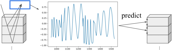
Figure 1: Spectrum generation on a 3-d semiconductor.

Most data augmentation techniques are designed for classification tasks and not necessarily for regression. Data augmentation techniques for classification including image processing (e.g., flipping or rotating) and generative models (e.g., GAN (Goodfellow et al. 2014) and VAE (Kingma and Welling 2014)) are not designed for regression tasks (see Sec. 5 for more details). More recently, Mixup (Zhang et al. 2018) is a popular data augmentation technique that is primarily used for classification, but can also be used for regression. The idea of Mixup is to mix two examples by linear interpolation and use it to estimate the label of any examples in between. There is theoretical evidence that Mixup regularizes the model being trained (Carratino et al. 2020; Zhang et al. 2021). Recently, various versions of Mixup (Verma et al. 2019; Yun et al. 2019; Kim, Choo, and Song 2020; Kim et al. 2021) have been proposed to train and calibrate the model better. Although Mixup can be used as is for regression, it is not equally effective because taking linear interpolations may sometimes do more harm than good to the model’s performance. The reason is that interpolating examples when the label space is continuous may result in arbitrarily-incorrect labels as illustrated in Fig. 2(a).

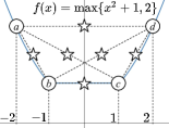
(a)

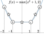
(b)

Figure 2: A comparison between Mixup (Zhang et al. 2018) and RegMix on a small regression dataset where each example (circle) is associated with a single-dimensional feature (x-axis). (a) Mixup takes a linear interpolation of all possible example pairs. Unfortunately, the mixed examples (stars) do not properly reflect the function $f$ (blue plot) where some labels are arbitrarily incorrect. (b) RegMix learns for each example how many nearest neighbors it should be mixed with. As a result, each example is only mixed with its 1- or 2-nearest neighbors to better reflect $f$.

We propose RegMix, a data mixing augmentation framework that is effective for regression tasks by limiting distances between mixing examples. Unlike existing theoretical works on Mixup for regression (Zhang et al. 2021; Carratino et al. 2020; Wu et al. 2020), RegMix assumes that linear interpolations when mixing examples are only effective within certain data distances. The distance limit may vary by example, and we formulate the problem of learning for each example how many nearest neighbors it should be mixed with, which we hereby refer to as a kNN mixing policy. RegMix employs a framework that searches for these policies that lead to the lowest model losses on a validation set using reinforcement learning (RL) (Zoph and Le 2017), although other search algorithms like evolution (Ho et al. 2019) can be used as well. Our approach is inspired by the AutoAugment framework (Cubuk et al. 2019), which searches image augmentation policies for classification. A key difference is that AutoAugment searches for the best augmentation operators that are applied to the entire data, while RegMix finds the number of neighbors to mix for each example. Fig. 2(b) shows how limiting the nearest neighbors to mix is better than mixing with all neighbors as in Mixup.

Experiments conducted on real and synthetic datasets show that RegMix outperforms baselines, especially when the mixing must be done selectively. RegMix is designed to improve model performance with more computation than simply mixing examples, so we also suggest using it has a post-hoc method after model training when the extra model performance gain makes a difference.

2 Limitations of Mixup in Regression

In this section, we explain why Mixup in classification has limitations in a regression setting in more detail. The original version of Mixup (Zhang et al. 2018) is to take a linear interpolation between any pair of examples $x_{i}$ and $x_{j}$ with the labels $y_{i}$ and $y_{j}$ to produce the new example $\lambda x_{i}+(1-\lambda)x_{j}$ with the label $\lambda y_{i}+(1-\lambda)y_{j}$ where $\lambda\sim Beta(\alpha,\alpha)$. According to Zhang et al. (2018), mixing all examples outperforms Empirical Risk Minimization on many classification datasets since the mixed examples have a regularization effect that prevents overfitting. On the other hand, mixing examples may cause manifold intrusion  (Guo, Mao, and Zhang 2019) where the mixed label is in the wrong label manifold and thus confuses the model.

In regression, however, the degree of manifold intrusion may be worse than classification due to the continuous label space. Since the possible number of label values is infinite, it is easier for a label to be incorrect. And the greater the distance between examples, the more likely the error is significant. For example, mixing the points $a$ and $d$ in Fig. 2(a) results in a label nowhere near the true label. In Sec. 4.3, we observe on real datasets that larger data distances lead to increased label errors and thus worse model performance.

Our key approach is thus to limit the data distance to improve Mixup for regression. If the regression model is continuous and two examples are close enough, the mixed label will be closer to the actual label when using linear interpolation. We provide a simple analysis in the supplementary. Even if the true function is not continuous (e.g., identical examples having different labels), we contend that limiting the data distances for mixing turns out to be an effective solution in practice.

3 Methodology: RegMix

The goal of RegMix is to identify which examples to mix with which nearest neighbors. Instead of finding the actual distance limits themselves, we solve the identical problem of finding the number of nearest neighbors to mix per example to reduce the search space. A naïve solution is to use Bayesian Optimization (BO) (Mockus 1974), but BO is known to be difficult to scale to high dimensions (Frazier 2018) and is thus not suitable in our setting where the number of parameters is the same as the dataset size. Instead, we use RL to find the policies.

3.1 Framework

Let $\mathcal{D}=\{(x_{i},y_{i})\}_{i=1}^{S}\sim P$ be the training set where $x_{i}\in X$ is a $d$-dimensional input example, and $y_{i}\in Y$ is an $e$-dimensional label. Let $\mathcal{D}^{v}=\{(x_{i}^{v},y_{i}^{v})\}_{i=1}^{V}\sim P^{t}$ be the validation set, where $P^{t}$ is the distribution of the test set, which is not necessarily the same as $P$. Let $f_{\phi}$ be a regression model, and $L$ the loss function that returns a performance score comparing $f_{\phi}(x_{i})$ with the true label $y_{i}$ using Mean Square Error (MSE) loss. We assume a list $N$ of possible nearest neighbors (NNs) based on data distance that can be mixed with an example. For instance, $N$ could contain the options {0 NN, 4 NNs, 8 NNs}. Notice that the “0 NN” option means that no mixing occurs because it is not beneficial to model performance. The more fine-grained the kNN options are, the more precisely RegMix can determine the optimal number of NNs to mix per example. On the other hand, there are diminishing returns because the optimization itself may become more difficult (see Sec. 4.4).

RegMix’s framework in Fig. 3 is similar to AutoAugment and neural architecture search (NAS) (Zoph and Le 2017) where a controller is trained to generate kNN mixing policies for all the examples in $\mathcal{D}$. The policies are then sampled probabilistically following the distributions of the softmax layers and used to augment $\mathcal{D}$ and train $f_{\phi}$. The models are then evaluated on $\mathcal{D}^{v}$, and the losses are used to update the controller. Alg. 1 shows the pseudocode of RegMix. Unlike typical RL settings where an episode consists of a sequence of dependent steps, in our setting an episode consists of independent steps because the controller can reach a goal after taking only one action (i.e., sampling kNN mixing policies). As a result, we can sample policies and compute model losses in parallel (lines 4–8). The collected losses are then used to compute the rewards and update the controller (lines 9–14).

Figure 3: RegMix’s workflow using two possible controllers. Assuming that mixing an example with its neighbors influences subsequent examples, an RNN-based controller can be used to predict the kNN mixing policies for an example sequence. Alternatively, if we do not explicitly model influence, then an MLP-based controller can be used to predict the kNN mixing policies for all examples at once.

Algorithm 1 Pseudocode of RegMix.

Input: training set $\mathcal{D}$, validation set $\mathcal{D}^{v}$, time horizon $T$
Initialize: controller $C$, moving average $\delta$ = 0, trajectory $\tau$, loss set $s$
Output: kNN mixing policies

1:  repeat

2:     $\tau$ = {}, $s$ = {};

3:     for $i=1\ldots T$ do {Can run in parallel}

4:        Initialize $\phi$;

5:        Sample kNN mixing policies $P$ from $C$ 

6:        Train $f_{\phi}$ with $\phi$ on $\mathcal{D}\cup Mix(\mathcal{D},P)$ 

7:        $Loss=\frac{1}{V}\sum_{i=1}^{V}L(f_{\phi}(x_{i}^{v}),y_{i}^{v})$ 

8:        Add $Loss$ to $s$;

9:     for $i=1\ldots T$ do

10:        $Loss$ = $s$[$i$];

11:        $r=\frac{1}{Loss}$ - $\delta$;

12:        Add $\{P,r\}$ to $\tau$;

13:        $\delta$ = 0.95$\delta$ + 0.05$\frac{1}{Loss}$;

14:     Update controller with $\tau$;

15:  until convergence

3.2 Controller Design

The controllers in the previous works AutoAugment (Cubuk et al. 2019) and NAS (Zoph and Le 2017) use recursive neural networks (RNNs) because of the sequential nature of the predictions to make. In AutoAugment, a policy consists of a sequence of operations on images that should be performed in a certain order (e.g., equalize and then rotate). In NAS, a model architecture consists of components that are connected in some sequence as well (e.g., elementwise multiplication followed by a ReLU activation function). Using an RNN is thus a natural choice in these cases.

For RegMix’s augmentation, there is no pre-determined sequence among examples, but one example mixing with its neighbors might “influence” the kNN mixing policies of other examples. For instance, if there are three examples $a$, $b$, and $c$ that are close together, and $a$ mixes with $b$, then $b$ may not have to mix with $a$ or even $c$ for the best model performance. If the examples can be ordered where examples that influence each other are close by, then an RNN can be used to determine the best kNN values for the sequence of examples. RegMix’s RNN-based controller (Fig. 3, controller on the left) consists of a sequence of LSTM (Hochreiter and Schmidhuber 1997) cells with softmax layers for the ordered examples similar to AutoAugment and NAS where the result of one cell is used as the input of the next. To find an ordering among examples, one can use dimensionality reduction or any other sorting method.

However, if there is no obvious ordering of examples, then an RNN may not be the ideal architecture. In Sec. 4.4 and Fig. 6, we observe that RegMix selectively mixes examples, but there are still quite a few examples that mix with most of the other examples. Mixing such an example may affect many other examples at the same time instead of the next example in some sequence. Here it is better to avoid specifically capturing the direction of influence as in an RNN.

We thus propose a more light-weight controller based on a multi-layer perceptron (MLP) instead of an RNN (Fig. 3, controller on the right) where the goal is to predict the best kNN mixing policies of all examples at once. Here the input does not play a role, and we fix it to a vector of 1’s. Also, there is one output node with a softmax layer per example. In Sec. 4.4, we show that using an MLP controller has similar model performances as when using an RNN controller.

Finding the optimal policy involves taking the gradient of the objective function $J(\theta)=\mathbb{E}_{\pi_{\theta}}[R]$ where $\pi$ is the policy, $\theta$ is the parameters of the controller, and $R$ is the reward function. We would like to minimize the regression model loss on a validation set when mixing a batch of examples. However, the validation loss is computed using the regression model, which does not involve $\theta$. Hence we cannot analytically compute the differential of the reward function with respect to $\theta$. In addition, there is no training data on how mixing each example affects the model performance.

We thus use Proximal Policy Optimization (PPO) (Schulman et al. 2017), which is one of the state-of-the-art on-policy algorithms and is also used in AutoAugment. We use PPO for convenience, and any actor-critic method like A3C (Mnih et al. 2016) can be used as well. In order to minimize the loss, we use the inverse of loss (i.e., $\frac{1}{\text{loss}}$) as the reward function. For stable learning, we employ an exponential moving average of previous rewards as the baseline function to reduce variance.

4 Experiments

We provide experimental results for RegMix. We evaluate regression models on separate test sets and repeat all model trainings five times. We use PyTorch (Paszke et al. 2017), and all experiments are performed using Intel Xeon Silver CPUs and NVidia RTX GPUs.

4.1 Experimental Settings

Measures

To measure accuracy, we use RMSE = $\sqrt{\frac{1}{n}\sum^{n}_{i=1}(y_{i}-\hat{y}_{i})^{2}}$, which is the absolute difference between predicted labels and true labels where a lower value is better. To measure the distance between examples, we use Euclidean distance.

Datasets

We use three real and one synthetic datasets. The NO2 emissions dataset (Aldrin 2004) contains traffic and meteorological information around roads. The features include cars per hour, wind speed, temperature, and others. The label is the NO2 concentration. The Bike UCI dataset (Dua and Graff 2017) contains climate and temporal information to predict the number of bikes in demand where the features include temperature, humidity, rainfall, and season. We take a random subset of the original dataset. The Product dataset obtained through a collaboration with a major tech company contains spectrum data that is generated using the procedure described in Sec. 1 and illustrated in Fig. 1 on 20-layer 3-d semiconductors. We also use a public synthetic dataset (DACON Co., Ltd. 2020) (Synthetic) since the Product dataset is proprietary. Here a simulator generates spectrum data using the same procedure as Product assuming 4-layer 3-d semiconductors. We provide more details in the supplementary.

Table 1 compares the four datasets in more detail. NO2 and Product have the lowest and highest dimensions, respectively, and Synthetic has the largest size. Although Product’s dimensionality is considered large for applications using spectrum data, there are datasets of even higher dimensions (e.g., large images or spatio-temporal data), and evaluating RegMix on them is an interesting future work. We also note that the data sizes are intentionally small as it is critical to show that RegMix performs well for small datasets. Finally, there are no personal identifiers.

Table 1: Settings for the four datasets.

Dataset	Data dim.	Label dim.	Train. set size	Val. set size
NO2	7	1	200	100
Bike	12	1	300	200
Product	580	20	300	200
Synthetic	226	4	600	400

RegMix Settings

As a default, we evaluate RegMix using the MLP controller for all results. When using an MLP controller, we use an MLP with 4 hidden layers and set the number of nodes per hidden layer to be [100, 100, 100, 100] for the four datasets with a learning rate of 0.002. When using an RNN controller, we use an embedding layer to adjust the dimension of inputs and LSTM cells with a hidden state size of 100. We use a learning rate of $\alpha=0.0005$. For the regression model $f_{\phi}$, we use an MLP using hyperparameters shown in Table 2. We also evaluate using other models in the supplementary, and the overall performance results are similar. We use layer normalization (Ba, Kiros, and Hinton 2016) for the Product and Synthetic datasets.

Table 2: Settings for regression models on the four datasets.

Dataset	MLP structure	Learning rate	Batch size
NO2	[512, 256]	0.0001	32
Bike	[512, 256]	0.0001	64
Product	[512, 256, 64]	0.0001	64
Synthetic	[2048, 1024, 512, 256]	0.001	64

When running Alg. 1, we set the time horizon $T$ to 20 and run lines 4–8 in parallel using multi-processing. For the controller, we employ an exponential moving average of previous rewards with a weight of 0.95 as the baseline function in order to improve the performance and stability of RL. To encourage exploration, we add an entropy term into the loss with a weight of 0.01. We use the Adam optimizer for all MLP or RNN trainings. When mixing examples, we sample $\lambda\sim Beta(\alpha,\alpha)$ with $\alpha=100$, which turns out to work well for regression tasks as we show in Sec. 4.4. We generate the kNN options using linear or exponential series. For the possible numbers of NNs for NO2, our default setting is the exponential series of integers $\{0\}\cup\{2^{i}|i\in[0,7]\}$ (i.e., $|N|=9$). For Bike, Product, and Synthetic, the default series are $\{0\}\cup\{4^{i}|i\in[0,4]\}$, $\{0\}\cup\{4^{i}|i\in[0,4]\}$, and $\{0\}\cup\{2^{i}|i\in[0,9]\}$, respectively.

Baselines

We employ six baselines. First, we train a regression model on the labeled data without any data augmentation (“Vanilla”). Next, we faithfully implement the Mixup algorithm (Zhang et al. 2018) where all example pairs can be mixed (“Mixup”). We also implement AdaMixup (Guo, Mao, and Zhang 2019) and Manifold Mixup (Verma et al. 2019), which are state-of-the-art Mixup techniques for classification that are also applicable to regression. We also compare with two simplified versions of RegMix where we use a global $k$ NN (“Global kNN”) or data distance $d$ threshold (“Global Distance”) for mixing examples with their nearest neighbors. The $k$ and $d$ parameters are tuned using Bayesian Optimization (Mockus 1974).

4.2 A Simple Evaluation on 1D Data

As an exercise, we validate RegMix’s internal workings on an expanded 1-dimensional synthetic dataset based on Fig. 2. We generate 10 training examples using the same equation $y=\max\{x^{2}+1,2\}$ with varying densities. We use the kNN options {0, 1, 2, 4, 8}. Fig. 4 shows that RegMix mixes examples in ranges that are sparse, but not too sparse. The RMSE of a model trained on the data drops from 5.770 to 5.489 compared to not using RegMix.

Figure 4: RegMix results on 1D dataset.

4.3 Data Distance Impact on Mixed Labels

We empirically show that the greater the data distance between two examples, the more the interpolated labels are inconsistent with the distribution of the training data. Given a dataset, we first train a regression model. We then generate mixed examples and compute the RMSE between their interpolated labels and the labels predicted by the regression model. While the regression model is not perfect, the relative trend of the error gives sufficient insight. Fig. 5(a) indeed shows increasing label errors for larger data distances for the three real datasets NO2, Bike, and Product. We also train regression models on top of augmented training sets where we only mix examples within certain distance ranges. Figs. 5(b)–5(d) show the model performances using RMSE for the three real datasets when mixing examples with different ranges of distances. Although the results vary by dataset, the overall trend is that increasing the data distance eventually causes the RMSE to increase to the extent that it is not worth mixing examples anymore.

(a) Label RMSE

(b) NO2

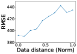
(c) Bike

(d) Product

Figure 5: Label and Model RMSEs for the three real datasets (lower RMSE is better) when mixing examples with different ranges of (normalized) distances. (a) Mixing larger distances leads to higher label RMSEs. (b)-(d) Mixing larger distances also leads to higher model RMSE values.

4.4 Performance Results

Table 3: RMSE results on all the real and synthetic datasets. Six baselines are compared with RegMix: (1) Vanilla; (2) Mixup (Zhang et al. 2018); (3) AdaMixup (Guo, Mao, and Zhang 2019); (4) Manifold Mixup (Verma et al. 2019); (5) Global kNN; and (6) Global Distance.

Dataset	Method	RMSE
NO2	Vanilla	$0.5441_{\pm 0.0004}$
	Mixup	$0.5401_{\pm 0.0013}$
	AdaMixup	$0.5397_{\pm 0.0005}$
	Manifold Mixup	$0.5381_{\pm 0.0038}$
	Global kNN (k=85)	$0.5470_{\pm 0.0009}$
	Global Dist. (d=0.81)	$0.5415_{\pm 0.0017}$
	RegMix	$\textbf{0.5248}_{\pm 0.0015}$
Bike	Vanilla	$393.45_{\pm 0.9049}$
	Mixup	$393.36_{\pm 1.8376}$
	AdaMixup	$391.62_{\pm 1.2527}$
	Manifold Mixup	$399.44_{\pm 0.7082}$
	Global kNN (k=68)	$388.81_{\pm 1.4053}$
	Global Dist. (d=0.41)	$388.43_{\pm 1.5282}$
	RegMix	$\textbf{368.86}_{\pm 3.0689}$
Product	Vanilla	$1.4100_{\pm 0.0042}$
	Mixup	$1.2310_{\pm 0.0107}$
	AdaMixup	$1.2293_{\pm 0.0105}$
	Manifold Mixup	$1.2894_{\pm 0.0042}$
	Global kNN (k=91)	$1.2625_{\pm 0.0102}$
	Global Dist. (d=0.32)	$1.2500_{\pm 0.0172}$
	RegMix	$\textbf{1.1948}_{\pm 0.0023}$
Synthetic	Vanilla	$15.6838_{\pm 0.2790}$
	Mixup	$13.8358_{\pm 0.0912}$
	AdaMixup	$13.7602_{\pm 0.0789}$
	Manifold Mixup	$14.0457_{\pm 0.1067}$
	Global kNN (k=61)	$13.7587_{\pm 0.0493}$
	Global Dist. (d=0.35)	$14.0860_{\pm 0.0875}$
	RegMix	$\textbf{13.4935}_{\pm 0.0913}$

We compare RegMix with the six baselines using the settings in Table 1. Table 3 shows the results for all the datasets. RegMix consistently outperforms all the baselines in terms of regression model performance, which demonstrates that it is able to pinpoint which examples should be mixed with how many kNNs. Fig. 6 shows which kNN options are frequently used by RegMix on all the datasets. When reading the histograms, keep in mind that the x-axis is an exponential series instead of a linear one. The y-axis is the frequency ratio ranging from 0 to 1. For Fig. 6(a), the frequency ratios are high for small kNN values and gradually lower for larger kNN values. This result is consistent with Fig. 5(b) where mixed examples with the longer distance increase RMSE. Fig. 6(b) has a similar distribution as Fig. 6(a) and is consistent with Fig. 5(c). Fig. 6(c)’s histogram is more uniform, which means that the larger kNN values have relatively higher frequencies compared to the NO2 and Bike datasets. This result is consistent with Fig. 5(d), where mixing is actually helpful for a wide range of data distances. Finally, Fig. 6(d) has a similar distribution as Fig. 6(c).

We further compare RegMix and Mixup on the Product dataset by plotting the model training convergence speeds on top of the augmented data (Fig. 7(a)). For Mixup, we evaluate two scenarios: when we use the entire mixed data or take a random sample of the mixed data that has the same size as RegMix’s augmented data for a fair comparison. As a result, the convergence is much faster when the model is trained on RegMix’s augmented data.

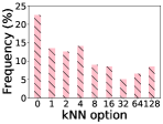
(a) NO2

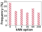
(b) Bike

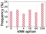
(c) Product

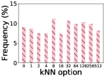
(d) Synthetic

Figure 6: kNN option frequency histograms for all datasets.

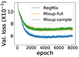
(a) Training convergence

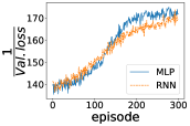
(b) Reward

Figure 7: (a) Model training convergence comparison on the Product dataset. (b) Rewards when using the MLP and RNN controllers on the Product dataset.

K Nearest Neighbor Options

We investigate how changing the kNN options $N$ affects RegMix’s performance in Table 4. For each dataset, we compare its default series with other possible series. We also fix the entire runtime by using the same number of epochs, so we only need to compare the model performances. We observe that providing more kNN options improves RegMix’s performance, but only to a certain extent. Adding options unnecessarily may actually result in lower performances as the best options are more difficult to find within the same time. Hence, RegMix performs best with a modest number of options.

Table 4: RegMix performances when using different kNN options on all datasets.

Dataset	kNN Options (Default = $\dagger$)	RMSE
NO2	$\{0\}\cup\{4^{i}|i\in[0,3]\}$	$0.5357_{\pm 0.0020}$
	$\{0\}\cup\{2^{i}|i\in[0,7]\}^{\dagger}$	$0.5248_{\pm 0.0015}$
	$\{0\}\cup\{10i|i\in[1,19]\}$	${0.5317}_{\pm 0.0011}$
Bike	$\{0\}\cup\{8^{i}|i\in[0,2]\}$	$378.02_{\pm 2.6582}$
	$\{0\}\cup\{4^{i}|i\in[0,4]\}^{\dagger}$	$368.86_{\pm 3.0689}$
	$\{0\}\cup\{2^{i}|i\in[0,8]\}$	$370.68_{\pm 0.6302}$
Product	$\{0\}\cup\{8^{i}|i\in[0,2]\}$	$1.2276_{\pm 0.0051}$
	$\{0\}\cup\{4^{i}|i\in[0,4]\}^{\dagger}$	$1.1948_{\pm 0.0023}$
	$\{0\}\cup\{2^{i}|i\in[0,8]\}$	$1.1954_{\pm 0.0100}$
Synthetic	$\{0\}\cup\{8^{i}|i\in[0,3]\}$	$13.7498_{\pm 0.0449}$
	$\{0\}\cup\{2^{i}|i\in[0,9]\}^{\dagger}$	${13.4935}_{\pm 0.0913}$
	$\{0\}\cup\{30i|i\in[1,19]\}$	$13.5510_{\pm 0.0916}$

Comparison with RNN Controller

We compare RegMix using the default MLP controller with RegMix that uses the RNN controller in Table 5 using the three real datasets. To clearly observe the RNN controller’s performance depending on the example ordering in the RNN, we consider two scenarios where (1) the examples are ordered after dimensionality reduction to one dimension using PCA (F.R.S. 1901) and (2) the examples are ordered randomly. As a result, there is no significant difference in model performances among the three approaches, which suggests that any influence among examples when mixing with neighbors is either minor or difficult to capture. As discussed in Sec. 3.2, we suspect that there is no easy way to model the influence by ordering the examples. Fig. 7(b) shows that the reward trends for the two controllers are similar as well.

Table 5: RegMix performances when using an MLP or RNN controller on the three real datasets. When using an RNN controller, we either (1) sort the examples using dimensionality reduction or (2) order them randomly.

Dataset	Controller	RMSE
NO2	MLP	$0.5248_{\pm 0.0015}$
	RNN (dim. reduction)	$0.5277_{\pm 0.0031}$
	RNN (rand. selection)	$0.5279_{\pm 0.0004}$
Bike	MLP	$368.86_{\pm 3.0689}$
	RNN (dim. reduction)	$368.03_{\pm 3.5014}$
	RNN (rand. selection)	$370.22_{\pm 1.3731}$
Product	MLP	$1.1948_{\pm 0.0023}$
	RNN (dim. reduction)	$1.1943_{\pm 0.0065}$
	RNN (rand. selection)	$1.1963_{\pm 0.0075}$

Varying $\alpha$

In Fig. 8(a), we vary $\alpha$ to adjust the Beta distribution from which we sample $\lambda$ for the Product dataset. As a result, an $\alpha$ of at least 100 results in the best model performances where $\lambda$ is very close to 0.5. The results for the other real datasets are similar and shown in the supplementary. We suspect that generating examples in the middle of two examples helps the regularization the most for regression.

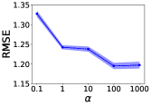
(a) $\alpha$ impact

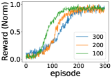
(b) Convergence speed

Figure 8: (a) RegMix performances using different $\alpha$ values on the Product dataset. (b) RegMix’s reward convergences on different amounts of Product data.

Other Regression Models

We also evaluate RegMix using a LightGBM (Ke et al. 2017) model (Table 6) and observe similar performance improvements as in Table 3. Hence, RegMix is also effective on models beyond MLPs.

Table 6: RegMix using a LightGBM (Ke et al. 2017) model.

Dataset	Model	Method	RMSE
NO2	LightGBM	Vanilla	$0.5334$
		Mixup	$0.5467$
		RegMix	0.5258
Bike	LightGBM	Vanilla	$385.31$
		Mixup	$335.15$
		RegMix	311.84

4.5 Convergence Speed and Post-hoc Method

We evaluate the convergence speed of RegMix on different amounts of Product data (Fig. 8(b)). The number of epochs needed for convergence increases for larger dataset sizes. In terms of runtime, RegMix takes hours to converge. Although RegMix can be viewed as expensive, the gained model performance can be worth the effort in real applications because data augmentation is a one-time cost that can run in batch mode. We discuss how to possibly improve RegMix’s runtime in the supplementary.

RegMix can also be used as a “post-hoc” step in model development where one first trains a model including hyperparameter tuning and then further train the model on the augmented data from RegMix using the same hyperparameters, if an extra gain in model performance is critical. We perform the same experiments as in Table 3 running RegMix post-hoc and observe that the RMSE values for RegMix are near identical as those in Table 3: 0.5286 for NO2, 375.57 for Bike, 1.2073 for Product, and 13.7943 for Synthetic.

5 Related Work

Data augmentation is essential for model performance (Park et al. 2019; Zhang et al. 2018; Krizhevsky, Sutskever, and Hinton 2012; Simard, Steinkraus, and Platt 2003), but there has been much more emphasis on classification than regression. There are largely three approaches: generative models, policies, and Mixup techniques. Generative models including GANs (Goodfellow et al. 2014) and VAEs (Kingma and Welling 2014) are popular in classification where the idea is to generate realistic data that cannot be distinguished from the real data by a discriminator. However, a major assumption is that the labels of the generated examples are the same, which does not necessarily hold in a regression setting where most examples may have different labels. Another approach is to find policies (Cubuk et al. 2019; Ratner et al. 2017; Ho et al. 2019; Cubuk et al. 2020; Lim et al. 2019; Hataya et al. 2020), which specify fixing rules for transforming the data while maintaining the label value. For example, image processing policies may flip, rotate, or adjust the brightness of images to generate new valid images (Zagoruyko and Komodakis 2016; Krizhevsky, Sutskever, and Hinton 2012). However, these policies usually target image classification or object detection tasks. In a regression setting, the same transformed examples may now have different unknown labels, making them unsuitable for training.

Mixup (Verma et al. 2019; Yun et al. 2019; Kim, Choo, and Song 2020; Kim et al. 2021) takes the alternative approach of generating both data and labels together by mixing existing examples with different labels using linear interpolations (Chapelle et al. 2000; Wu et al. 2020). Mixup can also be used in a regression setting, and there are analytical results on how it is effective by regularizing the model (Carratino et al. 2020; Zhang et al. 2021). However, our key observation is that mixing distant examples may actually be detrimental to model performance. RegMix shows better performance than Mixup by carefully choosing for each example which nearest neighbors to mix.

Within reinforcement learning (Sutton and Barto 2018; Kaelbling, Littman, and Moore 1996), we are interested in policy searching methods (Neumann and Peters 2015) where our goal is to find the best policy for mixing examples. In particular, RegMix’s framework is inspired by the recent AutoAugment framework (Cubuk et al. 2019; Lim et al. 2019; Hataya et al. 2020), which uses PPO (Schulman et al. 2017) to search for data augmentation policies that dictate how to modify existing examples to generate additional training data for image classification. In comparison, we solve the completely different problem of data augmentation for regression where we extend Mixup and find the best kNN neighbors to mix for each example.

6 Conclusion

We proposed RegMix, which is to our knowledge the first Mixup-based data augmentation framework for regression tasks utilizing distance information. We observe that mixing distant examples may not be beneficial and even detrimental to model performance. Hence, RegMix extends Mixup by determining the nearest neighbors to mix for each example using reinforcement learning where the objective is to minimize the regression model’s loss on a validation set. In our experiments, we showed that RegMix outperforms various data augmentation baselines for regression by effectively selecting among a modest number of nearest neighbor options.

7 Acknowledgment

Sung Yoon Ryu, Soo Seok Lee, and Gwang Nae Gil of Samsung Electronics provided the Product dataset and key insights on the 3-d semiconductor application. This work is supported by the Samsung Electronics’ University R$\&$D program [Algorithm advancement and reliability-enhancing technique development for spectrum data-based deep learning] and a Kwon Oh-Hyun Assistant Professorship.

Appendix A Appendix

A.1 Mixup Analysis for Cont. Regression Model

Suppose that the regression model $f$ is continuous where $\lim_{x\rightarrow c}f(x)=f(c)$ for any $x$ and $c$ within the domain of $f$. We show that a short-enough data distance sufficiently reduces the label distance as well. Given $f$’s domain $D$ and $\lim_{x\rightarrow c}f(x)=L$, the following is known to hold: $\forall\epsilon,\exists\delta$ s.t. $\forall x\in D$, if $|x-c|<\delta$, then $|f(x)-L|<\epsilon$. We can use this result to prove that $\forall\epsilon,\exists\delta$ s.t. $\forall x_{i},x_{j}\in D$, if $\alpha x_{i}+(1-\alpha)x_{j}=c$, $0\leq\alpha\leq 1$, and $|x_{i}-x_{j}|<\delta$ then the absolute difference between the mixed example’s $x_{j}$ value and $L$ is small where $|\alpha f(x_{i})+(1-\alpha)f(x_{j})-L|=|\alpha(f(x_{i})-L)+(1-\alpha)(f(x_{j})-L)|\leq\alpha|f(x_{i})-L|+(1-\alpha)|f(x_{j})-L|<\alpha\epsilon+(1-\alpha)\epsilon=\epsilon$. While this analysis does not cover all edge cases (e.g., identical examples having different labels), it does give an intuition why limiting the data distances for mixing is a reasonable solution.

A.2 More Experimental Settings

We continue describing our experimental settings from Sec. 4. When constructing the Synthetic dataset, recall that we take a subset of the entire DACON challenge dataset (DACON Co., Ltd. 2020). While the the range of thicknesses for the full datasets is [10, 300] for all four layers, we only use examples with thicknesses within the range [10, 100]. The purpose is to reduce the training time while still making a clear comparison between RegMix and the other methods.

A.3 More Experiments on $\alpha$ Impact

We continue showing RegMix performances for different $\alpha$ values of Beta distribution on NO2 and Bike datasets in Fig 9(a) and Fig 9(b). As a result, using an $\alpha$ of at least 100 results in the lowest RMSE.

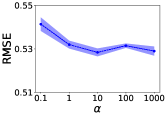
(a) $\sf NO2$

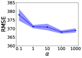
(b) $\sf Bike$

Figure 9: RegMix performances for different $\alpha$ values of the Beta distribution for sampling $\lambda$ on (a) NO2 and (b) Bike datasets.

A.4 Improving RegMix’s Runtime

We would also like to further improve RegMix’s runtime by possibly adapting techniques from efficient versions of AutoAugment like Fast AutoAugment (Lim et al. 2019) or Faster AutoAugment (Hataya et al. 2020). These methods view data augmentation as filling missing data points in the training data and skip the iterative full training process. However, the methods require large amounts of training data to train a model that accurately estimates the training data distribution. In our setup where the training data is small, the trained distribution will overfit to the training data, making these techniques less effective. Utilizing other scalable techniques is an interesting future work.

References

- Aldrin (2004) Aldrin, M. 2004. CMU StatLib Dataset. http://lib.stat.cmu.edu/datasets/. Accessed: 2022-08-15.
- Ba, Kiros, and Hinton (2016) Ba, J. L.; Kiros, J. R.; and Hinton, G. E. 2016. Layer Normalization. CoRR, abs/1607.06450.
- Carratino et al. (2020) Carratino, L.; Cissé, M.; Jenatton, R.; and Vert, J. 2020. On Mixup Regularization. CoRR, abs/2006.06049.
- Chapelle et al. (2000) Chapelle, O.; Weston, J.; Bottou, L.; and Vapnik, V. 2000. Vicinal Risk Minimization. In NIPS, 416–422.
- Cubuk et al. (2019) Cubuk, E. D.; Zoph, B.; Mane, D.; Vasudevan, V.; and Le, Q. V. 2019. AutoAugment: Learning Augmentation Strategies From Data. In CVPR, 113–123.
- Cubuk et al. (2020) Cubuk, E. D.; Zoph, B.; Shlens, J.; and Le, Q. V. 2020. Randaugment: Practical automated data augmentation with a reduced search space. In CVPR, 3008–3017. IEEE.
- DACON Co., Ltd. (2020) DACON Co., Ltd. 2020. Challenge on Semiconductor Thin Film Thickness Analysis. https://dacon.io/competitions/official/235554/data/. Accessed: 2022-08-15.
- Dua and Graff (2017) Dua, D.; and Graff, C. 2017. UCI Machine Learning Repository.
- Frazier (2018) Frazier, P. I. 2018. A tutorial on Bayesian optimization. arXiv preprint arXiv:1807.02811.
- F.R.S. (1901) F.R.S., K. P. 1901. LIII. On lines and planes of closest fit to systems of points in space. The London, Edinburgh, and Dublin Philosophical Magazine and Journal of Science, 2(11): 559–572.
- Goodfellow et al. (2014) Goodfellow, I. J.; Pouget-Abadie, J.; Mirza, M.; Xu, B.; Warde-Farley, D.; Ozair, S.; Courville, A. C.; and Bengio, Y. 2014. Generative Adversarial Nets. In NIPS, 2672–2680.
- Guo, Mao, and Zhang (2019) Guo, H.; Mao, Y.; and Zhang, R. 2019. MixUp as Locally Linear Out-of-Manifold Regularization. In AAAI, 3714–3722.
- Hataya et al. (2020) Hataya, R.; Zdenek, J.; Yoshizoe, K.; and Nakayama, H. 2020. Faster AutoAugment: Learning Augmentation Strategies Using Backpropagation. In Vedaldi, A.; Bischof, H.; Brox, T.; and Frahm, J., eds., ECCV, volume 12370, 1–16.
- Ho et al. (2019) Ho, D.; Liang, E.; Chen, X.; Stoica, I.; and Abbeel, P. 2019. Population Based Augmentation: Efficient Learning of Augmentation Policy Schedules. In ICML, 2731–2741.
- Hochreiter and Schmidhuber (1997) Hochreiter, S.; and Schmidhuber, J. 1997. Long Short-Term Memory. Neural Comput., 9(8): 1735–1780.
- Kaelbling, Littman, and Moore (1996) Kaelbling, L. P.; Littman, M. L.; and Moore, A. W. 1996. Reinforcement Learning: A Survey. J. Artif. Int. Res., 4(1): 237–285.
- Ke et al. (2017) Ke, G.; Meng, Q.; Finley, T.; Wang, T.; Chen, W.; Ma, W.; Ye, Q.; and Liu, T. 2017. LightGBM: A Highly Efficient Gradient Boosting Decision Tree. In NeurIPS, 3146–3154.
- Kim et al. (2021) Kim, J.; Choo, W.; Jeong, H.; and Song, H. O. 2021. Co-Mixup: Saliency Guided Joint Mixup with Supermodular Diversity. In ICLR.
- Kim, Choo, and Song (2020) Kim, J.-H.; Choo, W.; and Song, H. O. 2020. Puzzle mix: Exploiting saliency and local statistics for optimal mixup. In ICML, 5275–5285. PMLR.
- Kingma and Welling (2014) Kingma, D. P.; and Welling, M. 2014. Auto-Encoding Variational Bayes. In ICLR.
- Krizhevsky, Sutskever, and Hinton (2012) Krizhevsky, A.; Sutskever, I.; and Hinton, G. E. 2012. ImageNet Classification with Deep Convolutional Neural Networks. In Bartlett, P. L.; Pereira, F. C. N.; Burges, C. J. C.; Bottou, L.; and Weinberger, K. Q., eds., NIPS, 1106–1114.
- Lim et al. (2019) Lim, S.; Kim, I.; Kim, T.; Kim, C.; and Kim, S. 2019. Fast AutoAugment. In NeurIPS, 6662–6672.
- Mnih et al. (2016) Mnih, V.; Badia, A. P.; Mirza, M.; Graves, A.; Lillicrap, T. P.; Harley, T.; Silver, D.; and Kavukcuoglu, K. 2016. Asynchronous Methods for Deep Reinforcement Learning. In ICML, 1928–1937.
- Mockus (1974) Mockus, J. 1974. On Bayesian Methods for Seeking the Extremum. In Proceedings of the IFIP Technical Conference, 400–404. Berlin, Heidelberg: Springer-Verlag. ISBN 3540071652.
- Neumann and Peters (2015) Neumann, G.; and Peters, J. 2015. Policy search: Methods and applications. In ICML.
- Park et al. (2019) Park, D. S.; Chan, W.; Zhang, Y.; Chiu, C.; Zoph, B.; Cubuk, E. D.; and Le, Q. V. 2019. SpecAugment: A Simple Data Augmentation Method for Automatic Speech Recognition. In Kubin, G.; and Kacic, Z., eds., Interspeech, 2613–2617.
- Paszke et al. (2017) Paszke, A.; Gross, S.; Chintala, S.; Chanan, G.; Yang, E.; DeVito, Z.; Lin, Z.; Desmaison, A.; Antiga, L.; and Lerer, A. 2017. Automatic Differentiation in PyTorch. In NIPS Autodiff Workshop.
- Ratner et al. (2017) Ratner, A. J.; Ehrenberg, H. R.; Hussain, Z.; Dunnmon, J.; and Ré, C. 2017. Learning to Compose Domain-Specific Transformations for Data Augmentation. In NeurIPS, 3236–3246.
- Schulman et al. (2017) Schulman, J.; Wolski, F.; Dhariwal, P.; Radford, A.; and Klimov, O. 2017. Proximal Policy Optimization Algorithms. CoRR, abs/1707.06347.
- Simard, Steinkraus, and Platt (2003) Simard, P. Y.; Steinkraus, D.; and Platt, J. C. 2003. Best Practices for Convolutional Neural Networks Applied to Visual Document Analysis. In ICDAR, 958–962. IEEE Computer Society.
- Sutton and Barto (2018) Sutton, R. S.; and Barto, A. G. 2018. Reinforcement Learning: An Introduction. A Bradford Book. ISBN 0262039249.
- Verma et al. (2019) Verma, V.; Lamb, A.; Beckham, C.; Najafi, A.; Mitliagkas, I.; Lopez-Paz, D.; and Bengio, Y. 2019. Manifold mixup: Better representations by interpolating hidden states. In ICML.
- Wu et al. (2020) Wu, S.; Zhang, H. R.; Valiant, G.; and Ré, C. 2020. On the Generalization Effects of Linear Transformations in Data Augmentation. In ICML, volume 119, 10410–10420. PMLR.
- Yun et al. (2019) Yun, S.; Han, D.; Chun, S.; Oh, S. J.; Yoo, Y.; and Choe, J. 2019. CutMix: Regularization Strategy to Train Strong Classifiers With Localizable Features. In ICCV, 6022–6031.
- Zagoruyko and Komodakis (2016) Zagoruyko, S.; and Komodakis, N. 2016. Wide Residual Networks. In Wilson, R. C.; Hancock, E. R.; and Smith, W. A. P., eds., BMVC.
- Zhang et al. (2018) Zhang, H.; Cissé, M.; Dauphin, Y. N.; and Lopez-Paz, D. 2018. mixup: Beyond Empirical Risk Minimization. In ICLR.
- Zhang et al. (2021) Zhang, L.; Deng, Z.; Kawaguchi, K.; Ghorbani, A.; and Zou, J. 2021. How Does Mixup Help With Robustness and Generalization? In ICLR.
- Zoph and Le (2017) Zoph, B.; and Le, Q. V. 2017. Neural Architecture Search with Reinforcement Learning. In ICLR.