Mean Force Based Temperature Accelerated Sliced Sampling: Efficient Reconstruction of High Dimensional Free Energy Landscapes

Abstract

Temperature Accelerated Sliced Sampling (TASS) is an efficient method to compute high dimensional free energy landscapes. The original TASS method employs the Weighted Histogram Analysis Method (WHAM) which is an iterative post-processing to reweight and stitch high dimensional probability distributions in sliced windows that are obtained in the presence of restraining biases. The WHAM necessitates that TASS windows lie close to each other for proper overlap of distributions and span the collective variable space of interest. On the other hand, increase in number of TASS windows implies more number of simulations, and thus it affects the efficiency of the method. To overcome this problem, we propose herein a new mean-force (MF) based reweighting scheme called TASS-MF, which enables accurate computation with a fewer number of windows devoid of the WHAM post-processing. Application of the technique is demonstrated for alanine di- and tripeptides in vacuo to compute their two- and four-dimensional free energy landscapes, the latter of which is formidable in conventional umbrella sampling and metadynamics. The landscapes are computed within a kcal mol^-1 accuracy, ensuring a safe usage for broad applications in computational chemistry.

I Introduction

Free energy barriers, and free energy difference between reactants and products, are the two thermodynamic quantities of interest in predicting the spontaneity and kinetics of the chemical reactions and other physio-chemical transformations. In this respect, computing free energy landscape of such processes as a function of few collective variables (CVs) is a commonly employed strategy.Peters (2017); Tuckerman (2010); Vanden-Eijnden (2009); Christ et al. (2010); Bonella et al. (2012); Valsson et al. (2016); Awasthi and Nair (2019); Paul et al. (2019) Molecular Dynamics (MD) combined with enhanced sampling techniques are widely used for this purpose. Enhanced sampling methods are essential to accelerate the transitions from one free energy basin to another. Accelerating CVs by bias potentialsTorrie and Valleau (1974); Darve and Pohorille (2001); Laio and Parrinello (2002); Barnett and Naidoo (2009) and high-temperatureRosso et al. (2002); Tuckerman (2010); Maragliano and Vanden-Eijnden (2006); Abrams and Tuckerman (2008) are some of strategies proposed for this purpose. Alternative approaches include accelerating the system dynamics by flattening the underlying potential energy landscape by bias potentials, replica–exchange based global-tempering and other generalized ensemble methods.Tuckerman (2010); Voter (1997); Affentranger et al. (2006); Liu et al. (2005); Gao (2008); Grubmüller (1995); Hamelberg et al. (2004); Mitsutake et al. (2001); Itoh and Okumura (2012); Morishita et al. (2012); Hayami et al. (2019)

One of the simplest approaches that employ biased sampling of CVs is Umbrella Sampling (US).Torrie and Valleau (1974); Kästner (2011) Here a bias potential,

$$W_{h}^{\rm b}(s)=\frac{1}{2}k\left[s(\mathbf{R})-\xi_{h}\right]^{2},\enspace h=1,\cdots,M\enspace,$$ (1)

is applied to restrain the CV $s(\mathbf{R})$ at $M$ discrete values $\{\xi_{h}\}$. In the above, $\mathbf{R}$ is the set of atomic coordinates, and $k$ is the coupling constant. Biased canonical probability distribution of $s$ obtained for each umbrella window is given as,

$$\tilde{P}_{h}(s^{\prime}) = \frac{1}{\tilde{Z}}\int d\mathbf{R}\,e^{-\beta\left[U(\mathbf{R})+W_{h}^{\rm b}(s)\right]}\,\delta\left(s(\mathbf{R})-s^{\prime}\right)$$ (2)

$$\equiv \left<\delta\left(s(\mathbf{R})-s^{\prime}\right)\right>_{W_{h}^{\rm b}}$$

where

$$\tilde{Z}=\int d\mathbf{R}\,e^{-\beta\left[U(\mathbf{R})+W_{h}^{\rm b}(s)\right]}\enspace,$$

$U$ is the potential energy, $\beta=\left(k_{\rm B}T\right)^{-1}$, $k_{\rm B}$ is the Boltzmann constant, and $T$ is the temperature. In the above $\left<\cdots\right>_{W_{h}^{\rm b}}$ specifies the ensemble average in the presence of the bias $W_{h}^{\rm b}$. The Weighted Histogram Analysis Method (WHAM)Ferrenberg and Swendsen (1989); Kumar et al. (1992) is then employed to combine the biased probability distributions and reweight them to obtain final (unbiased) distribution $P(s)$. In WHAM, this is done by computing

$$P(s)=\frac{\sum_{h=1}^{M}n_{h}{\tilde{P}_{h}(s)}}{\sum_{h=1}^{M}n_{h}g_{h}\exp{[-\tilde{\beta}W_{h}^{b}(s)]}}$$ (3)

where,

$$g_{h}^{-1}=\int{ds\exp{[-\tilde{\beta}W_{h}^{\rm b}(s)]}}\,{P}(s)$$

is unknown. An iterative procedure is employed, where the iteration begins with $g_{h}=1$, and improved at every step based on the $P(s)$ computed in the previous step. For the correct convergence of $P(s)$, a proper overlap of $\tilde{P}_{h}(s)$ with its neighboring distributions is essential. It is to be noted that the width of the distribution $\tilde{P}_{h}(s)$ depends on the value of $k$; Higher the value of $k$, more accurate will be the free energy estimate. On the other hand, increasing the value of $k$ will make the distribution narrower, and thereby the extent of overlap between the neighboring distributions will become smaller. As a result, more umbrella windows have to be used with high values of $k$ for obtaining accurate results. Further, when dealing with high dimensional CV-space, long MD simulations are required to achieve sufficient overlap of distributions. Due to this limitation, US is often used to explore only a one-dimensional or a part of a two-dimensional CV-space.

Several techniques were proposed to improve the limitations of US.Bartels and Karplus (1997); Hooft et al. (1992); Mezei (1987); Wojtas-Niziurski et al. (2013); Awasthi and Nair (2017); Kästner and Thiel (2005); Kästner (2011) Temperature Accelerated Sliced Sampling (TASS) method Awasthi and Nair (2017, 2019) extends the US method to high dimensions by combining it with temperature accelerated molecular dynamics (TAMD)/driven adiabatic free energy dynamics (d-AFED) Rosso et al. (2005); Maragliano and Vanden-Eijnden (2006); Abrams and Tuckerman (2008) and metadynamics Laio and Parrinello (2002) methods. TASS uses the extended Lagrangian,

$$\mathcal{L}_{h}({\bf R,\dot{R},z,\dot{z})} = \mathcal{L}^{0}({\bf R,\dot{R}})+$$ (4)

$$\sum_{\alpha=1}^{n}\left[\frac{1}{2}{\mu_{\alpha}}{{\bf\dot{z}}_{\alpha}}^{2}+\frac{\kappa_{\alpha}}{2}(s_{\alpha}({\bf R})-z_{\alpha})^{2}\right]-$$

$$W_{h}^{\rm b}(z_{1})-V^{\rm b}(\overline{\mathbf{z}},t),$$

$$h=1,\cdots,M,$$

where $\mathcal{L}^{0}$ is the original Lagrangian of the system, $\mu_{\alpha}$ is the mass of the auxiliary degree of freedom $z_{\alpha}$, and $\kappa_{\alpha}$ is the restraining force of the spring that couples the $z_{\alpha}$ and the corresponding CV $s_{\alpha}$. Two kinds of bias potentials $W_{h}^{\rm b}(z_{1})$ and $V^{\rm b}(\overline{\mathbf{z}},t)$, are added on the auxiliary degrees of freedom. The bias $W_{h}^{\rm b}(z_{1})$ is the umbrella bias potential given by Eqn. 1, acting on the auxiliary variable $z_{1}$. A metadynamics bias,Laio and Parrinello (2002); Iannuzzi et al. (2003) $V^{\rm b}(\overline{\mathbf{z}},t)$ is applied along a small set of auxiliary variables $\overline{\mathbf{z}}\equiv(z_{2},\cdots,z_{m})$, and $m\leq n$. The dimension of the auxiliary vector space ${\overline{\mathbf{z}}}$ is less than or equal to that of ${\bf z}$. It is preferred to choose

$$V^{\rm b}(\overline{\mathbf{z}},t)=\sum_{\tau<t}w_{\tau}\,\exp{\left[-\frac{{\left\{\overline{\mathbf{z}}-\overline{\mathbf{z}}_{\tau}\right\}}^{2}}{2(\delta z)^{2}}\right]}$$ (5)

with

$$w_{\tau}=\omega_{0}\exp\left[{-\frac{V^{b}(\overline{\mathbf{z}}_{\tau},\tau)}{k_{B}\Delta T}}\right],$$ (6)

and $\overline{\mathbf{z}}_{\tau}\equiv\overline{\mathbf{z}}(\tau)$ as in well-tempered metadynamics (WT-MTD).Barducci et al. (2008); Dama et al. (2014) In the above, $w_{\tau}$ is the height of the Gaussian deposited at time $\tau$, $\delta z$ is the width of the Gaussian, and $\Delta T$ is a parameter. In TASS, the auxiliary variables are thermostatted to $\tilde{T}$ K, while the physical system is thermostatted to $T$ K, with $\tilde{T}\gg T$. Here we define, $\tilde{\beta}=\left(k_{\rm B}\tilde{T}\right)^{-1}$ and $\beta=\left(k_{\rm B}T\right)^{-1}$. The probability distribution for each TASS window $h$ is first calculated as

$$\tilde{P}_{h}(\mathbf{z}^{\prime})=\frac{\int dt\,A_{h}(t)\,\prod_{\alpha}^{n}\,\delta\left(z_{\alpha}(t)-z^{\prime}_{\alpha}\right)}{\int dt\,A_{h}(t)}$$ (7)

where

$$A_{h}(t)=\exp\left[\tilde{\beta}\left\{V_{h}^{\rm b}\left(\overline{\mathbf{z}}_{t},t\right)-c_{h}(t)\right\}\right]$$ (8)

and

$$c(t)=\frac{1}{\tilde{\beta}}\ln\left[\frac{\int d\overline{\mathbf{z}}\,\exp\left[\tilde{\beta}\gamma V^{\rm b}(\overline{\mathbf{z}},t)\right]}{\int d\overline{\mathbf{z}}\,\exp\left[\tilde{\beta}(\gamma-1)V^{\rm b}(\overline{\mathbf{z}},t)\right]}\right]\enspace.$$ (9)

As next, high dimensional probability distribution $\tilde{P}(\mathbf{z})$ is obtained by Eqn. 3. Free energy surface at temperature $T$ is obtained as

$$F(\mathbf{z})=-\frac{1}{\tilde{\beta}}\ln\tilde{P}(\mathbf{z})$$ (10)

as in TAMD/d-AFED. The main advantage of TASS is that a large number of collective variables can be used by virtue of the temperature acceleration of the auxiliary space. Umbrella bias provides a way to achieve a directed or controlled sampling when used along an appropriate CV. The method also permits to use different transverse coordinates for different umbrella windows depending on the requirement. This is possible as free energy slices are independently computed in the corresponding windows.

However, reconstruction of free energy surfaces by WHAM encounters problems when dealing with large number of CVs for the reasons discussed earlier. In this paper, we propose a way to reconstruct high dimensional free energy surfaces in TASS simulations using a mean force based method, and dispense the computationally inefficient WHAM approach. Most importantly, the proposed method does not involve an iterative scheme, unlike WHAM. The new method is quite general, and is applicable not only to TASS, but also to US and WT-MTD simulations.

II Theory

Mean force based computation of free energies is core to several techniques.Carter et al. (1989); Sprik and Ciccotti (1998); Khavrutskii et al. (2008); Darve and Pohorille (2001); Chen et al. (2012); Morishita et al. (2017) Mean force based reconstruction of free energy surfaces in the frame work of extended Lagrangian has been reported earlier for adaptive bias sampling (ABF) Darve (2007); Darve and Pohorille (2001); Darve et al. (2008); Lelièvre et al. (2007); Comer et al. (2015); Lesage et al. (2017), logarithmic mean-force dynamicsMorishita et al. (2012) TAMD/d-AFED, UFED and metadynamics.Chen et al. (2012); Cuendet and Tuckerman (2014) Such techniques use the gradient of the underlying free energy to compute free energy surfaces using thermodynamic integration as

$$F(z)=\int^{z}dz^{\prime}\left<\frac{dF}{dz^{\prime}}\right>\enspace.$$ (11)

Such integration become tricky with increasing dimensions. Using a basis set expansionChen et al. (2012) and artificial neural network representationSchneider et al. (2017) of free energy will be more efficient approaches to overcome such issues to some extent. Here we present an alternative method that suits the TASS approach, and is efficient for dealing with high dimensions. We will utilize the advantages of employing mean-forces to combine independently sampled probability distributions (or free energy slices) by the TASS Lagrangian (Eqn. 4) to reconstruct high-dimensional free energy surfaces. The challenge here is to reconstruct a high-dimensional free energy landscape where the CVs are differently biased.

First, we write the derivative of projected free energy, $F_{1}(z_{1})$, along the auxiliary variable $z_{1}$ in which the umbrella bias is active.

$$F_{1}(z_{1})=-\frac{1}{\tilde{\beta}}\ln P_{1}(z_{1})$$ (12)

where,

$$P_{1}(z_{1})=\int dz_{2}\cdots dz_{n}\,e^{-\tilde{\beta}F(z_{1},\cdots,z_{n})}$$ (13)

Since US bias is applied along $z_{1}$, the force at $z_{1}=\xi_{h}$ is given by

$$\left(\frac{dF_{1}}{dz_{1}}\right)_{\xi_{h}}=-{\left\langle k_{h}\left[z_{1}-\xi_{h}\right]\right\rangle}_{\xi_{h}},\enspace h=1,\cdots,M.$$ (14)

Note that, other approach could be to compute the mean-force on real CVs (i.e., $\mathbf{s}$, and not the auxiliary coordinates, $\mathbf{z}$), as in Ref. Chen et al. (2012). Since a subset of the auxiliary coordinates, $\overline{\mathbf{z}}$, is biased by time dependent metadynamics potential in the TASS formalism, we can relate,

$${\left\langle k_{h}\left[z_{1}-\xi_{h}\right]\right\rangle}_{\xi_{h}}=\frac{\int{d\mathbf{z}\;\left[k\left(z_{1}-\xi_{h}^{h}\right)\right]\;\exp\left[\tilde{\beta}\{V^{\rm b}(\overline{\mathbf{z}},t)-c(t)\}\right]}}{\int{d\mathbf{z}\;\exp\left[\tilde{\beta}\{V^{\rm b}(\overline{\mathbf{z}},t)-c(t)\}\right]}}$$ (15)

which in turn can be computed by the time average,

$$\frac{\int dt\,A(t)\,\left[k\left(z_{1}-\xi_{h}^{h}\right)\right]}{\int dt\,A(t)}$$ (16)

and the time dependent reweighting factor $A(t)$ is given by Eqn. 8. Employing these equations, we can compute projected free energy $F_{1}$ along $z_{1}$ from a TASS simulation as follows:

$$F_{1}(z_{1}) = \int^{z_{1}}dz_{1}^{\prime}\,\left(\frac{dF_{1}}{dz_{1}^{\prime}}\right)$$ (17)

$$\approx -\sum_{h=1}^{M^{\prime}-1}\Delta\xi_{h}\,\,w_{h}\left[g_{h}+g_{h+1}\right]\,\,$$

where

$$g_{h}=\langle k_{h}\left[z_{1}-\xi_{h}\right]\rangle_{\xi_{h}}\enspace.$$ (18)

Here, $M^{\prime}$ is the grid index corresponding to the CV value $z_{1}$. This integral can be computed in a straight forward manner using the trapezoidal rule, with $\Delta\xi_{h}=\xi_{h+1}-\xi_{h}$, and the integration weights $w_{h}=\frac{1}{2}$ for all the values of $h$. We stress that the above equation reconstructs only the projection of the free energy surface $F(\mathbf{z})$ along the US coordinate $z_{1}$, i.e. $F_{1}(z_{1})$. Now, the multidimensional free energy surface can related to $F_{1}(z_{1})$ as follows:

$$F(z_{1},\cdots,z_{n}) = -\frac{1}{\tilde{\beta}}\ln\,\left[e^{-\tilde{\beta}F(z_{1},\cdots,z_{n})}\right]$$ (19)

$$= -\frac{1}{\tilde{\beta}}\ln\left[\frac{P_{1}(z_{1})}{P_{1}(z_{1})}e^{-\tilde{\beta}F(z_{1},\cdots,z_{n})}\right]$$

$$= -\frac{1}{\tilde{\beta}}\ln P_{1}(z_{1})-\frac{1}{\tilde{\beta}}\ln\frac{e^{-\tilde{\beta}F(z_{1},\cdots,z_{n})}}{P_{1}(z_{1})}$$

$$= F_{1}(z_{1})-\frac{1}{\tilde{\beta}}\ln\frac{e^{-\tilde{\beta}F(z_{1},\cdots,z_{n})}}{\int dz_{2}\cdots dz_{n}\,e^{-\tilde{\beta}F(z_{1},\cdots,z_{n})}}$$

$$= F_{1}(z_{1})-\frac{1}{\tilde{\beta}}\ln\tilde{P}_{z_{1}}(z_{2},\cdots,z_{n})$$

$$= F_{1}(z_{1})+\Delta F_{z_{1}}(z_{2},\cdots,z_{n})$$

where,

$$\Delta F_{z_{1}}(z_{2},\cdots,z_{n})=-\frac{1}{\tilde{\beta}}\ln\tilde{P}_{z_{1}}(z_{2},\cdots,z_{n})$$ (20)

is the $n-1$ dimensional slice of the free energy surface at $z_{1}$, and $\tilde{P}_{z_{1}}$ is the corresponding slice of the probability distribution obtained at temperature $\tilde{T}$ K. We can use the relationship in Eqn. 19 to reconstruct the high dimensional free energy landscape, $F(\mathbf{z})\equiv F(z_{1},z_{2},\cdots,z_{n})$. Since in TASS, time dependent bias acts along a subset of the orthogonal CV space $z_{2},\cdots,z_{n}$, the reweighting approach as discussed in Eqn. 7 has to be used for obtaining unbiased distribution $\tilde{P}_{z_{1}}(z_{2},\cdots,z_{n})$ by binning. Interpolation schemes can be used to obtain free energy values between the grid points $\xi_{1},\cdots,\xi_{M}$ along $z_{1}$.

The procedure explained here does not require WHAM for stitching the free energy slices together to obtain high dimensional free energy surfaces. This approach which uses the mean-force will be denoted as TASS-MF and the WHAM based approach to reconstruct the TASS free energy surfaces will be called TASS-WHAM, hereafter.

In practice, we perform the following steps in reconstructing the high-dimensional free energy surface:

1. Perform TASS simulations for the windows $h=1,\cdots,M$ using the Lagrangian given in Eqn. 4.

2. Compute $\left\{V_{h}^{\rm b}\right\}$ and $\left\{c_{h}(t)\right\}$, for $h=1,\cdots,M$.

3. From the trajectory of the auxiliary variables, $z_{1},\cdots,z_{M}$, compute the one dimensional free energy profile $F_{1}(z_{1})$ using Eqn. 17.

4. Compute the high dimensional free energy slice for $z_{1}\in\left(\xi_{1},\cdots,\xi_{M}\right)$ using Eqn.20.

5. Reconstruct the high dimensional free energy surface employing Eqn. 19.

III Result and Discussion

III.1 Alanine Dipeptide in Vacuum

To demonstrate the accuracy of this method, free energy surface of alanine dipeptide in vacuo as a function of Ramachandran angles ($\phi,\psi$) was computed using various methods; see Fig. 1. The molecule was modelled by the ff14SB Maier et al. (2015) AMBER force field and MD simulations were performed by using AMBER 18Case et al. (2018) patched with the PLUMED interface. Bonomi et al. (2009) The same set of calculations was repeated using the PIMD code where the TASS method has been implemented.Ruiz-Barragan et al. (2016); Shiga (2020) The time step used for integrating the equations of motion is $1$ fs. We performed TASS simulations by applying umbrella bias along $\phi$ and WTMTD bias along $\psi$. Three sets of TASS simulations were executed by varying number of umbrella windows: (a) 40; (b) 30; (c) 20. The umbrella restraints were centered equal-distant in the domain $\phi\in(-\pi,\pi]$ and $k=239$ kcal mol^-1 rad^-2 was taken. For the Gaussian bias (Eqn. 5), we chose $w_{0}=0.57$ kcal mol^-1, $\delta z=0.05$ rad, $\Delta T=2700$ K, and the bias was updated every 500 fs. We took $\kappa=1258$ kcal mol^-1 rad^-2 and $\mu=50$ amu Å² rad^-2. Calculations were done at canonical ensemble with $T=300$ K, and an Langevin thermostat having a frictional coefficient of 0.1 fs^-1 was employed to control the temperature of the physical system. We used $\tilde{T}=1000$ K for the extended system, and the temperature of the extended variables was maintained using a separate massive Langevin thermostat with a frictional coefficient of 0.1 fs^-1. For each window, we performed 20 ns long production run. As reference free energy data, we performed a conventional WTMTD simulation for 100 ns, where the coordinates $\phi$ and $\psi$ were biased using a two-dimensional Gaussian bias-potential (as in Eqn. 5). We used $\Delta T=1500$ K, otherwise all the metadynamics parameters were the same as that in the TASS simulations.

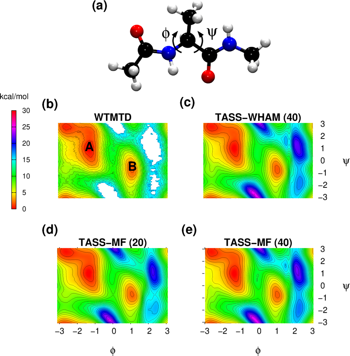
Figure 1: (a) Ball and stick representation of alanine dipeptide. $\phi$ and $\psi$ are the Ramachandran angles, specifically the torsional angle between atoms C-N-C_α-C and N-C_α-C-N, respectively, as shown in the figure. Color code: H (white), C (black), O(red), and N (blue). The free energy surface reconstructed in the $(\phi,\psi)$-space computed from (b) WTMTD (100 ns), and (c) TASS-WHAM with 40 equidistant windows are used as the reference data. The same computed using TASS-MF with 20 and 40 equidistant windows are shown in the subfigures (d), and (e). The contours are drawn for every 1 kcal mol^-1

In Figure 1(b-e), we have presented the free energy surfaces using WTMTD, TASS with WHAM based reweighting with equidistant 40 umbrella windows (TASS-WHAM (40)), and the new method presented here, i.e., using the mean-force (TASS-MF). TASS-MF reweighting was carried out with 40, 30 and 20 equidistant windows, and they are indicated as TASS-MF (40), TASS-MF (30), and TASS-MF (20), respectively. Clearly, the positions of the minima and saddles are exactly identical in all the landscapes; See Fig 1(b)-(e). A quantitative comparison of the free energy barriers on the $F(\phi,\psi)$ surface was carried out for WTMTD, TASS-WHAM, TASS-MF simulations; see Table 1. In the WTMTD simulations, free energy barriers A $\rightarrow$ B and B $\rightarrow$ A were converged to 9.7 and 8.0 kcal mol^-1, respectively; See Appendix B for convergence study. The same computed from TASS-WHAM converged to 9.4 and 7.8 kcal mol^-1 in 20 ns per window; see also Appendix B. The differences between the free energy barriers from the two simulations are less than 1 kcal mol^-1. Of great importance, the barriers computed from TASS-MF (40) with the same TASS windows agree well with the TASS-WHAM (40) data. The errors in the free energy barriers using TASS-MF (30), and TASS-MF (20) are also less than 1 kcal mol^-1. Further, the $L^{2}$ errors (Appendix A), computed by taking the WTMTD free energy surface as the reference were found to be less than 0.6 kcal mol^-1. It is to be noted that WHAM will not converge well with 30 and 20 umbrella windows.

Method	$\Delta F^{\ddagger}$ (kcal mol-1)		$L^{2}{\rm error}$ (kcal mol-1)
	A $\rightarrow$ B	B $\rightarrow$ A
WTMTD	9.7	8.0	0.0
TASS-WHAM	9.4	7.8	0.4
TASS-MF (40)	9.7	7.9	0.5
TASS-MF (30)	9.6	7.8	0.4
TASS-MF (20)	8.9	7.1	0.6

Table 1: Free energy barriers ($\Delta F^{\ddagger}$) for the transitions A $\rightarrow$ B and B $\rightarrow$ A computed from various methods. $L^{2}{\rm error}$ was calculated by taking WTMTD as reference.

III.2 Alanine tripeptide

To demonstrate the application of the method to high-dimensional free energy landscapes, we reconstructed the four dimensional free energy landscape of alanine tripeptide in vacuo as a function of four Ramachandran angles $(\phi_{1},\psi_{1},\phi_{2},\psi_{2})$; see Fig. 2(a). We note that the four-dimensional free energy surface was available in our calculation from TASS but not from WTMTD, since the latter was computationally prohibitive. Here, umbrella bias was applied along $\phi_{1}$, metadynamics bias was applied along $\phi_{2}$, while all the four CVs were enhanced sampled at high temperature as per the TASS formalism. Equilibration run for each window was carried out for about 1 ns followed by 40 ns of production run. All the parameters and simulation details for the TASS simulation were kept the same as in the case of alanine dipeptide except that $\mu$ was taken as $450$ amu Ų rad^-2. After carrying out the TASS simulation with four CVs $(\phi_{1},\psi_{1},\phi_{2},\psi_{2})$ the reconstructed four-dimensional free energy was projected along $(\phi_{1},\phi_{2})$, $(\phi_{1},\psi_{1})$ and $(\phi_{2},\psi_{2})$ spaces; see Figs. 2(b)-(e), 3, and 4. The performance of TASS-WHAM with 40 umbrella windows was compared with TASS-MF with 40, 30, and 20 windows. The comparison of the free energy barriers on the $F(\phi_{1},\phi_{2})$, $F(\phi_{1},\psi_{1})$, and $F(\phi_{2},\psi_{2})$ surfaces, computed from TASS-WHAM and TASS-MF simulations, are presented in Tables 2. The difference in the free energy barriers computed from TASS-WHAM (40) and TASS-MF (40) is not greater than 0.2 kcal mol^-1. Free energy barriers computed from TASS-MF using 40, 30, and 20 windows are agreeing within an acceptable margin of 1 kcal mol^-1. The $L^{2}$ errors in the $F(\phi_{1},\phi_{2})$ estimates by the TASS-MF calculations (by taking TASS-WHAM as the reference) are also less than or equal to 0.5 kcal mol^-1, and the highest error was observed for TASS-MF (20).

Method	$\Delta F^{\ddagger}$ (kcal mol-1)								$L^{2}{\rm error}$ (kcal mol-1)
	P $\rightarrow$ Q	Q $\rightarrow$ P	R $\rightarrow$ Q	Q $\rightarrow$ R	M $\rightarrow$ N	N $\rightarrow$ M	M′ $\rightarrow$ N′	N′ $\rightarrow$ M′
TASS-WHAM (40)	6.6	8.9	6.7	8.5	7.4	6.6	9.1	7.7	0.0
TASS-MF (40)	6.6	8.9	6.7	8.3	7.2	6.6	9.0	7.6	0.1
TASS-MF (30)	6.7	8.7	6.5	8.1	7.5	6.7	9.0	7.8	0.4
TASS-MF (20)	6.7	8.7	6.3	7.8	6.9	6.1	8.9	7.4	0.5

Table 2: Free energies barriers ($\Delta F^{\ddagger}$) for P $\rightarrow$ Q, Q $\rightarrow$ P, R $\rightarrow$ Q, and Q $\rightarrow$ R in $(\phi_{1},\phi_{2})$ space, M $\rightarrow$ N, N $\rightarrow$ M in ($\phi_{1}$,$\psi_{1}$) space, M^′ $\rightarrow$ N^′, and N^′ $\rightarrow$ M^′ in ($\phi_{2}$,$\psi_{2}$) space computed from various methods. $L^{2}{\rm error}$ was calculated for $F(\phi_{1},\phi_{2})$ by taking TASS-WHAM (40) as reference.

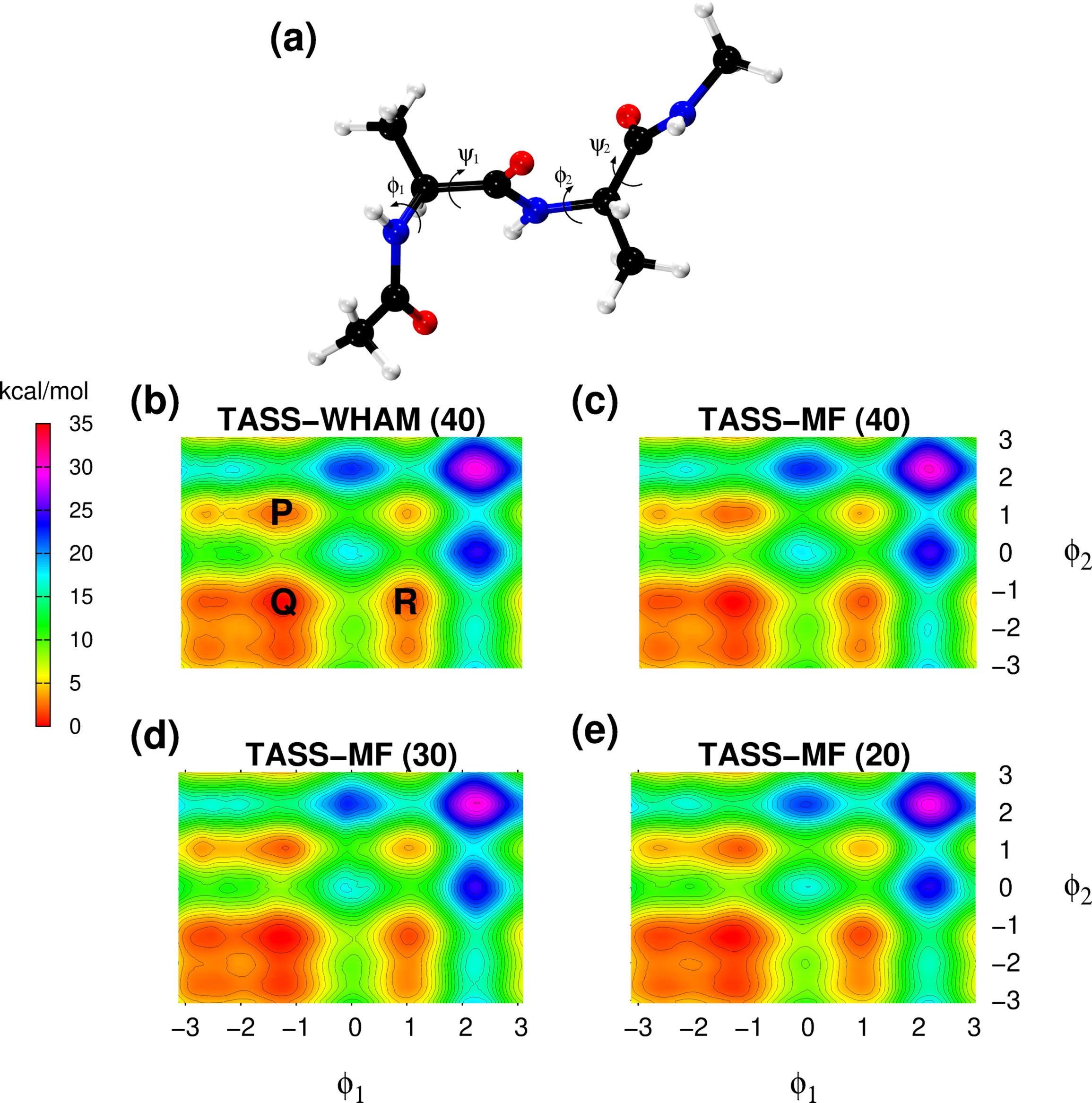
Figure 2: (a) Ball and stick representation of alanine tripeptide. The free energy surface reconstructed in the $(\phi_{1},\phi_{2})$-space computed from (b) WHAM-40 can be compared with those using the TASS-MF method with 40 (c), 30 (d), and 20 (e) equidistant windows. The contours are drawn for every 1 kcal mol^-1.

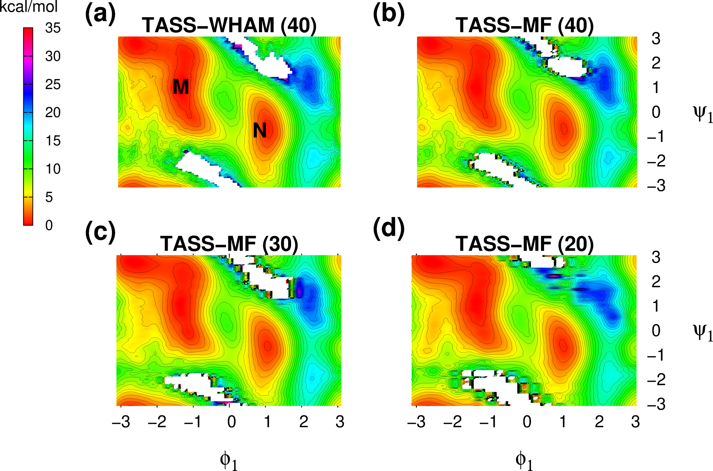
Figure 3: (a) The free energy surfaces $F(\phi_{1},\psi_{1})$ computed from TASS-WHAM with 40 equidistant windows is presented together with the same computed using TASS-MF with 40 (b), 30 (c) and 20 (d) equidistant windows. The contours are drawn for every 1 kcal mol^-1.

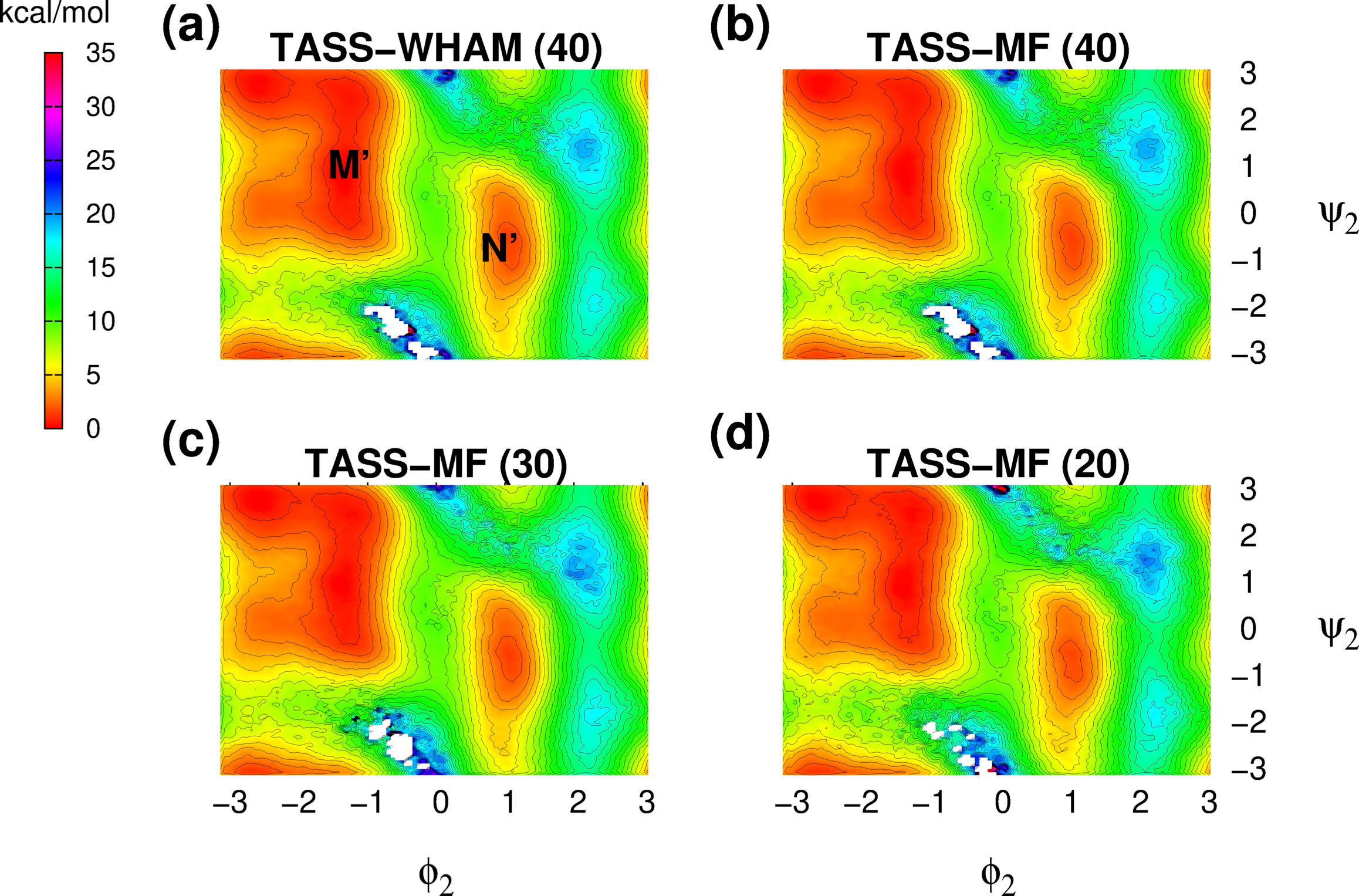
Figure 4: (a) The free energy surfaces $F(\phi_{2},\psi_{2})$ computed from TASS-WHAM with 40 equidistant windows is presented together with the same computed using TASS-MF with 40 (b), 30 (c) and 20 (d) equidistant windows. The contours are drawn for every 1 kcal mol^-1.

IV Conclusions

An efficient as well as computationally straightforward reweighing scheme for TASS is presented here. In this approach the high-dimensional free energy estimate is divided into two parts, in which the first part contains the free energy projected along the umbrella sampling coordinate, while the second term is the low-dimensional slice of the free energy surface. We show that the first term can be directly computed by integrating the reweighted mean force acting along the umbrella coordinate at the equilibrium position of the umbrella potential, whereas the second term can be obtained by binning and reweighting. The advantage of the new method is that WHAM iteration can be completely avoided in order to combine free energy slices. We demonstrated the accuracy of the method by reconstructing the free energy surfaces of alanine dipeptide and alanine tripeptide systems. The surfaces were computed accurately even with half the number of umbrella windows, with a maximum difference in free energy barriers not beyond than 0.5 kcal mol^-1 compared to that of TASS-WHAM. As the TASS-MF method proposed here permits us to perform reconstruction of high-dimensional free energy surfaces with much less number of umbrella windows, the method improves the efficiency of the TASS simulations.

Appendix A Calculation of Least Square Error: $L^{2}\mathrm{error}$ Chen et al. (2012)

$$L^{2}\mathrm{error}=\sqrt{\frac{1}{N}\sum_{i}^{N}[F(\mathbf{z}_{i})-F_{\mathrm{ref}}(\mathbf{z}_{i})]^{2}}$$ (21)

Here, $N$ is the total number of the grid points, $F(\mathbf{z}_{i})$ is the value of computed free energy for various methods and $F_{\mathrm{ref}}(\mathbf{z}_{i})$ is the value of reference free energy at $i^{\mathrm{th}}$ grid.

Appendix B Convergence of Free Energy Barriers: Alanine Dipeptide In Vaccuo

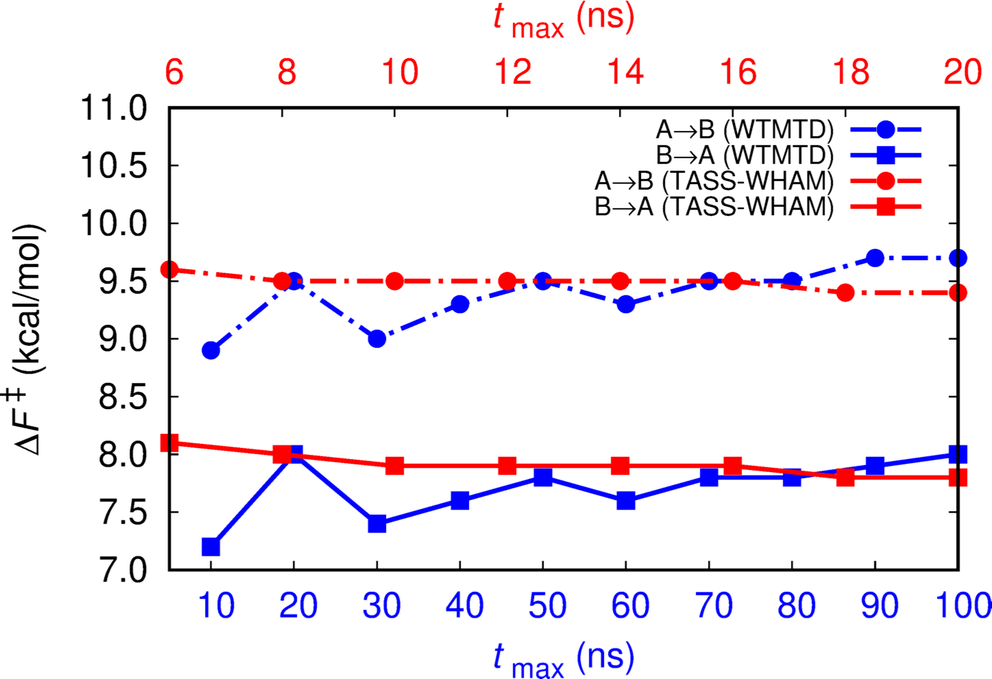
Figure 5: Convergence of free energy barriers ($\Delta F^{\ddagger}$) for A $\rightarrow$ B in WTMTD (blue circles) and TASS-WHAM (red circles) simulations is plotted together with that for B $\rightarrow$ A (blue/red squares). Here, $t_{\mathrm{max}}$ is the net simulation length in WTMTD and simulation time per umbrella window for TASS-WHAM (40 windows).

References

- Peters (2017) B. Peters, Reaction Rate Theory and Rare Events (Elsevier, Amsterdam, Netherlands, 2017).
- Tuckerman (2010) M. E. Tuckerman, Statistical Mechanics: Theory and Molecular Simulation, 1st ed. (Oxford University Press, Oxford, 2010).
- Vanden-Eijnden (2009) E. Vanden-Eijnden, J. Comput. Chem. 30, 1737 (2009).
- Christ et al. (2010) C. D. Christ, A. E. Mark, and W. F. van Gunsteren, J. Comput. Chem. 31, 1569 (2010).
- Bonella et al. (2012) S. Bonella, S. Meloni, and G. Ciccotti, Eur. Phys. J. B 85, 97 (2012).
- Valsson et al. (2016) O. Valsson, P. Tiwary, and M. Parrinello, Annu. Rev. Phys. Chem. 67, 159 (2016).
- Awasthi and Nair (2019) S. Awasthi and N. N. Nair, Wiley Interdisciplinary Reviews: Computational Molecular Science 9, e1398 (2019).
- Paul et al. (2019) S. Paul, N. N. Nair, and V. Harish, Mol. Sim. 45, 1273 (2019).
- Torrie and Valleau (1974) G. M. Torrie and J. P. Valleau, Chem. Phys. Lett. 28, 578 (1974).
- Darve and Pohorille (2001) E. Darve and A. Pohorille, J. Chem. Phys. 115, 9169 (2001).
- Laio and Parrinello (2002) A. Laio and M. Parrinello, Proc. Natl. Acad. Sci. U.S.A 99, 12562 (2002).
- Barnett and Naidoo (2009) C. B. Barnett and K. J. Naidoo, Mol. Phys. 107, 1243 (2009).
- Rosso et al. (2002) L. Rosso, P. Mináry, Z. Zhu, and M. E. Tuckerman, J. Chem. Phys. 116, 4389 (2002).
- Maragliano and Vanden-Eijnden (2006) L. Maragliano and E. Vanden-Eijnden, Chem. Phys. Lett. 426, 168 (2006).
- Abrams and Tuckerman (2008) J. B. Abrams and M. E. Tuckerman, J. Phys. Chem. B 112, 15742 (2008).
- Voter (1997) A. F. Voter, Phys. Rev. Lett. 78, 3908 (1997).
- Affentranger et al. (2006) R. Affentranger, I. Tavernelli, and E. E. Di Iorio, J. Chem. Theory Comput. 2, 217 (2006).
- Liu et al. (2005) P. Liu, B. Kim, R. A. Friesner, and B. J. Berne, Proc. Nat. Acad. Sci. 102, 13749 (2005).
- Gao (2008) Y. Q. Gao, J. Chem. Phys. 128, 064105 (2008).
- Grubmüller (1995) H. Grubmüller, Phys. Rev. E 52, 2893 (1995).
- Hamelberg et al. (2004) D. Hamelberg, J. Mongan, and J. A. McCammon, J. Chem. Phys. 120, 11919 (2004).
- Mitsutake et al. (2001) A. Mitsutake, Y. Sugita, and Y. Okamoto, Peptide Science 60, 96 (2001).
- Itoh and Okumura (2012) S. G. Itoh and H. Okumura, J. Chem. Theory Comput. 9, 570 (2012).
- Morishita et al. (2012) T. Morishita, S. G. Itoh, H. Okumura, and M. Mikami, Phys. Rev. E 85, 066702 (2012).
- Hayami et al. (2019) T. Hayami, J. Higo, H. Nakamura, and K. Kasahara, Journal of Computational Chemistry 40, 2453 (2019).
- Kästner (2011) J. Kästner, WIREs Comput. Mol. Sci. 1, 932 (2011).
- Ferrenberg and Swendsen (1989) A. M. Ferrenberg and R. H. Swendsen, Phys. Rev. Lett. 63, 1195 (1989).
- Kumar et al. (1992) S. Kumar, J. M. Rosenberg, D. Bouzida, R. H. Swendsen, and P. A. Kollman, J. Comput. Chem. 13, 1011 (1992).
- Bartels and Karplus (1997) C. Bartels and M. Karplus, J. Comput. Chem. 18, 1450 (1997).
- Hooft et al. (1992) R. Hooft, B. Vaneijck, and J. Kroon, J. Chem. Phys. 97, 6690 (1992).
- Mezei (1987) M. Mezei, J. Comput. Phys. 68, 237 (1987).
- Wojtas-Niziurski et al. (2013) W. Wojtas-Niziurski, Y. Meng, B. Roux, and S. Bernéche, J. Chem. Phys. 9, 1885 (2013).
- Awasthi and Nair (2017) S. Awasthi and N. N. Nair, J. Chem. Phys. 146, 094108 (2017).
- Kästner and Thiel (2005) J. Kästner and W. Thiel, J. Chem. Phys. 123, 144104 (2005).
- Rosso et al. (2005) L. Rosso, J. B. Abrams, and M. E. Tuckerman, J. Phys. Chem. B 109, 4162 (2005).
- Iannuzzi et al. (2003) M. Iannuzzi, A. Laio, and M. Parrinello, Phys. Rev. Lett. 90, 238302 (2003).
- Barducci et al. (2008) A. Barducci, G. Bussi, and M. Parrinello, Phys. Rev. Lett. 100, 020603 (2008).
- Dama et al. (2014) J. F. Dama, M. Parrinello, and G. A. Voth, Phys. Rev. Lett. 112, 240602 (2014).
- Carter et al. (1989) E. Carter, G. Ciccotti, J. Hynes, and R. Karpal, Chem. Phys. Lett. 156, 472 (1989).
- Sprik and Ciccotti (1998) M. Sprik and G. Ciccotti, J. Chem. Phys. 109, 7737 (1998).
- Khavrutskii et al. (2008) I. V. Khavrutskii, J. Dzubiella, and J. A. McCammon, J. Chem. Phys. 128, 044106 (2008).
- Chen et al. (2012) M. Chen, M. A. Cuendet, and M. E. Tuckerman, J. Chem. Phys. 137, 024102 (2012).
- Morishita et al. (2017) T. Morishita, Y. Yonezawa, and A. M. Ito, Journal of Chemical Theory and Computation 13, 3106 (2017).
- Darve (2007) E. Darve, Free energy calculations, edited by C. Chipot and A. Pohorille (Springer-Verlag, Berlin, Heidelbarg, New York, 2007).
- Darve et al. (2008) E. Darve, D. Rodriguez-Gomez, and A. Pohorille, J. Chem. Phys. 128, 144120 (2008).
- Lelièvre et al. (2007) T. Lelièvre, M. Rousset, and G. Stoltz, J. Chem. Phys. 126, 134111 (2007).
- Comer et al. (2015) J. Comer, J. C. Gumbart, J. Hénin, T. Lelièvre, A. Pohorille, and C. Chipot, J. Phys. Chem. B 119, 1129 (2015).
- Lesage et al. (2017) A. Lesage, T. Lelièvre, G. Stoltz, and J. Hénin, J. Phys. Chem. B 121, 3676 (2017).
- Cuendet and Tuckerman (2014) M. A. Cuendet and M. E. Tuckerman, J. Chem. Theory Comput. 10, 2975 (2014).
- Schneider et al. (2017) E. Schneider, L. Dai, R. Q. Topper, C. Drechsel-Grau, and M. E. Tuckerman, Phys. Rev. Lett. 119, 150601 (2017).
- Maier et al. (2015) J. A. Maier, C. Martinez, K. Kasavajhala, L. Wickstrom, K. E. Hauser, and C. Simmerling, J. Chem. Theory Comput. 11, 3696 (2015).
- Case et al. (2018) D. A. Case, I. Y. Ben-Shalom, S. R. Brozell, D. S. Cerutti, T. E. Cheatham, III, V. W. D. Cruzeiro, T. A. Darden, R. E. Duke, D. Ghoreishi, M. K. Gilson, H. Gohlke, A. W. Goetz, D. Greene, R. Harris, N. Homeyer, Y. Huang, S. Izadi, A. Kovalenko, T. Kurtzman, T. S. Lee, S. LeGrand, P. Li, C. Lin, J. Liu, T. Luchko, R. Luo, D. J. Mermelstein, K. M. Merz, Y. Miao, G. Monard, C. Nguyen, H. Nguyen, I. Omelyan, A. Onufriev, F. Pan, R. Qi, D. R. Roe, A. Roitberg, C. Sagui, S. Schott-Verdugo, J. Shen, C. L. Simmerling, J. Smith, R. Salomon-Ferrer, J. Swails, R. C. Walker, J. Wang, H. Wei, R. M. Wolf, X. Wu, L. Xiao, D. M. York, and P. A. Kollman, AMBER 2018 (University of California, San Francisco, 2018).
- Bonomi et al. (2009) M. Bonomi, D. Branduardi, G. Bussi, C. Camilloni, D. Provasi, P. Raiteri, D. Donadio, F. Marinelli, F. Pietrucci, R. A. Broaglia, and M. Parrinello, Comput. Phys. Commun. 180, 1961 (2009).
- Ruiz-Barragan et al. (2016) S. Ruiz-Barragan, K. Ishimura, and M. Shiga, Chemical Physics Letters 646, 130 (2016).
- Shiga (2020) M. Shiga, PIMD version 2.4.0 (2020), https://ccse.jaea.go.jp/software/PIMD/index.en.html.