Early Science with the Large Millimeter Telescope: a 1.1 mm AzTEC Survey of Red-Herschel dusty star-forming galaxies

Abstract

We present LMT/AzTEC 1.1 mm observations of $\sim 100$ luminous high-redshift dusty star-forming galaxy candidates from the $\sim 600\,$sq.deg Herschel-ATLAS survey, selected on the basis of their SPIRE red far-infrared colours and with $S_{500\mu\rm m}=35-80$ mJy. With an effective $\theta_{\rm FWHM}\approx 9.5\,$ arcsec angular resolution, our observations reveal that at least 9 per cent of the targets break into multiple systems with SNR $\geq 4$ members (i.e. without considering close mergers). The fraction of multiple systems increases to $\sim 23$  per cent (or more) if some non-detected targets are multiples, as suggested by the data. Combining the new AzTEC and deblended Herschel photometry we derive photometric redshifts, IR luminosities, and star formation rates. While the median redshifts of the multiple and single systems are similar ($z_{\rm med}\approx 3.6$), the latter are skewed towards higher redshifts. Of the AzTEC sources $\sim 85$ per cent lie at $z_{\rm phot}>3$ while $\sim 33$  per cent are at $z_{\rm phot}>4$. This corresponds to a lower limit on the space density of ultra-red sources at $4<z<6$ of $\sim 3\times 10^{-7}\,\textrm{Mpc}^{-3}$ and a contribution to the obscured star-formation $\gtrsim 8\times 10^{-4}\,\textrm{M}_{\odot}\textrm{yr}^{-1}\textrm{Mpc}^{-3}$. Some of the multiple systems have members with photometric redshifts consistent among them suggesting possible physical associations. Given their angular separations, these systems are most likely galaxy over-densities and/or early-stage pre-coalescence mergers. Finally, we present 3mm LMT/RSR spectroscopic redshifts of six red-Herschel galaxies at $z_{\rm spec}=3.85-6.03$, two of them (at $z\sim 4.7$) representing new redshift confirmations. Here we release the AzTEC and deblended Herschel photometry as well as catalogues of the most promising interacting systems and $z>4$ galaxies.

1 Introduction

Taking advantage of a narrow atmospheric window at $\lambda\approx 850\,\mu\rm m$, around two decades ago, the first surveys taken at submillimeter wavelengths with the SCUBA camera —which now sits in the National Museum of Scotland in Edinburgh— confirmed the existence of a population of high-redshift dust-enshrouded star-forming galaxies (e.g. Smail et al. 1997; Barger et al. 1998; Hughes et al. 1998).

Thanks to the significant two-decade effort poured into determining the physical properties of these galaxies, it is now known that they show the most extreme star formation rates (SFR from 100’s to 1000’s M${}_{\odot}\,{\textrm{yr}}^{-1}$) in the Universe (modulo the possibility of a very top heavy stellar initial mass function, e.g. Zhang et al. 2018), have large stellar and dust masses ($\sim 10^{10-11}$ and $\sim 10^{8-9}$ M_⊙, respectively) with large gas mass reservoirs ($\sim 10^{10-11}$ M_⊙), and contribute significantly to the cosmic star formation rate density (see reviews by Casey, Narayanan & Cooray 2014 and Hodge & da Cunha 2020). These sources are also considered to be the progenitors of massive, quiescent galaxies observed at $z\approx 2-3$, which ultimately lead to the assembly of the massive elliptical galaxies observed in the local Universe (Toft et al. 2014; Simpson et al. 2014).

Nevertheless, despite their recognized importance in our understanding of galaxy formation and evolution, fundamental questions remain unanswered. For example, although the bulk of the population is known to lie at $z\approx 2-4$ (e.g. Aretxaga et al. 2003; Chapman et al. 2005; Aretxaga et al. 2007; Yun et al. 2012; Michałowski et al. 2012; Simpson et al. 2014; Koprowski et al. 2016; Brisbin et al. 2017; Zavala et al. 2018b; Simpson et al. 2020; Dudzevičiūtė et al. 2020), their distribution at high-redshifts ($z>4$) and its dependence with flux density remains unclear. Constraining the prevalence of these galaxies is crucial, for instance, to derive a complete census of the cosmic star formation rate density and to test our current models of cosmic structure formation, since these galaxies are expected to trace the assembly of the first massive dark matter halos in the Universe (Marrone et al. 2018).

An important step towards understanding the formation processes that built up these extreme galaxies relies on determining their triggering mechanisms and their star formation modes. Pioneering observational and theoretical studies concluded that the formation scenario of Sub-Millimeter Galaxies (SMGs) involves major and minor gas-rich mergers (e.g., Tacconi et al. 2006; Ivison et al. 2007; Bothwell et al. 2010; Engel et al. 2010; Narayanan et al. 2010). Nevertheless, subsequent theoretical work showed that early-stage mergers (pre-coalescence galaxy pairs), isolated star-forming disks, and even line-of-sight projections or gravitational lensing can also lead to these bright submm fluxes (e.g., Davé et al. 2010; Hayward et al. 2011; Narayanan et al. 2015). Although it is now clear that the population of dusty star-forming galaxies (DSFGs) may be rather heterogeneous (e.g. Hayward et al. 2018; Jiménez-Andrade et al. 2020), the relative importance of each component remains uncertain.

Characterizing these specifics requires sensitive and wide enough surveys to capture the rarest systems, which allow us to test the predictions from galaxy-formation models (e.g. Hayward 2013; Gruppioni et al. 2015; Lacey et al. 2016; Lagos et al. 2019; McAlpine et al. 2019).

The large-area surveys conducted with the Herschel Space Observatory (as well as the South Pole Telescope – SPT; Vieira et al. 2010) have already identified remarkable examples of such systems, including some of the most distant dusty galaxies currently known at $z\approx 6-7$ (Riechers et al. 2013; Fudamoto et al. 2017; Zavala et al. 2018a) and extreme galaxy over-densities (i.e. proto-cluster structures) in the early Universe (e.g. Ivison et al. 2013; Oteo et al. 2018; see Strandet et al. 2017 and Miller et al. 2018 for similar systems selected by the SPT). Part of this success relies on the availability of simultaneous observations at 250, 350, and $500\,\mu\rm m$ with SPIRE, which enable a straightforward selection criteria ($S_{250\mu\rm m}<S_{350\mu\rm m}<S_{500\mu\rm m}$) of high-redshift candidates known as ‘$500\mu\rm m$ risers’ or ‘red-Herschel galaxies’ (e.g. Pope & Chary 2010; Cox et al. 2011; Dowell et al. 2014; Asboth et al. 2016; Ivison et al. 2016; Donevski et al. 2018; Duivenvoorden et al. 2018; Ma et al. 2019; Bakx et al. 2020b).

Follow-up observations with higher angular resolutions at (ideally) longer wavelengths than those used to select these galaxies are, however, necessary as an intermediate step to identify and filter out possible contaminants, whilst providing more accurate positions for spectroscopic surveys. Previous works, as those discussed in more detail below, have focused on samples of red-Herschel sources followed-up with the SCUBA-2 camera at $850\,\micron$ ($\theta_{\rm FWHM}\approx 15\,$ arcsec), LABOCA at $870\,\micron$ ($\theta_{\rm FWHM}\approx 19\,$ arcsec; Dowell et al. 2014; Ivison et al. 2016; Asboth et al. 2016; Duivenvoorden et al. 2018; Donevski et al. 2018), or with higher angular resolution interferometric observations with ALMA, NOEMA and the SMA (e.g. Ma et al., 2019; Greenslade et al., 2020).

Here, we present $1.1\rm\,mm$ imaging, using the AzTEC camera (Wilson et al., 2008) on the Large Millimeter Telescope (LMT, Hughes et al. 2010) of a relatively large sample of 100 Herschel-selected galaxies. Additionally, we present 3mm spectra of 6 red-Herschel sources using the Redshift Search Receiver (RSR). We provide new redshifts for 2 of these sources (with $z\gtrsim 4.7$) and confirm the redshift of the other 4, which were already known (Fudamoto et al., 2017; Zavala et al., 2018a).

The 32-m illuminated surface of the telescope, at the time of the observations, provides an effective angular resolution of $\theta_{\rm FWHM}\approx 9.5\,$ arcsec, a factor of 4 better than Herschel at $500\,\mu\rm m$ ($\theta_{\rm FWHM}\approx 36\,$ arcsec). This angular resolution enables the identification of not only the most promising high-redshift candidates but also of physically interacting galaxies blended within the Herschel beam, as discussed below.

This paper is structured as follows: §2 describes the sample selection and AzTEC/RSR observations. The analysis of these images and the bulk of the results are presented in §3. This includes constraints on the multiplicity, as well as photometric redshift, luminosity, and SFR estimations. In §4 we identify and present sub-samples of the most promising high redshift candidates and physically interacting galaxies. Finally, the implications of these results in our general understanding of the properties of this population of galaxies are discussed in §5, where our conclusions are also summarized.

Throughout this paper, we assume a flat $\Lambda$CDM cosmology with $H_{0}=68\rm\,km\,s^{-1}\,Mpc^{-1}$ and $\Omega_{\Lambda}=0.69$ (Planck Collaboration et al. 2016), and the Chabrier (2003) initial mass function (IMF) for SFR estimations.

2 Sample and observations

2.1 Sample Selection

The Herschel Astrophysical Terahertz Large Area Survey (H-ATLAS, Eales et al., 2010; Valiante et al., 2016) is one of the largest surveys ($\sim 600\rm\,deg^{2}$) carried out with the Herschel Space Observatory. The thousands of sources detected at 250, 350 and $500\,\mu{\textrm{m}}$ in the South Galactic Pole (SGP), North Galactic Pole (NGP) and the Galaxy and Mass Assembly 9hr (G09), 12hr (G12) and 15hr (G15) fields, make H-ATLAS an ideal survey to search for rare high-redshift ($z\gtrsim 4$) dusty star-forming galaxies.

Our sample was taken from a parent sample of ultrared DSFGs obtained by Ivison et al. (2016), where a detailed description of the selection process is presented and summarized here. First, candidates at $>2.2\sigma$ were identified in the 250$\mu$m maps using the Multi-band Algorithm for source eXtraction (MADX; Maddox & Dunne, 2020). Then, PSFs with scaled flux densities at each band were subtracted from the SPIRE maps. Subsequently, a second and third set of candidates were generated by repeating the process and searching for $>2.4\sigma$ and $>3.5\sigma$ peaks in the 350$\mu$m and 500$\mu$m residual maps respectively. The final catalog of 7961 ultra-red sources includes only those detected at $\geq 3.5\sigma$ at 500$\mu$m and with $S_{500\mu\textrm{m}}/S_{250\mu\textrm{m}}\geq 1.5$ and $S_{500\mu\textrm{m}}/S_{350\mu\textrm{m}}\geq 0.85$. A sub-sample of 2725 ultrared candidates was eyeballed to find a reliable sample for ground-based observations. It is important to note that the eyeballing process rejected 22 per cent of the candidates which were heavily confused and whose flux densities (and therefore colours) were unreliable (see Ivison et al. 2016 for details).

This colour selected sources with spectral energy distributions (SEDs) that rise from 250 to $350\,\mu{\textrm{m}}$ and continue rising onwards to $500\mu{\textrm{m}}$ ($S_{250\rm\mu{\textrm{m}}}<S_{350\rm\mu{\textrm{m}}}<S_{500\mu{\textrm{m}}}$) are called ‘$500\mu{\textrm{m}}$ risers’ or red-Herschel sources. This technique enabled the identification of DSFGs up to $z\sim 6$ (e.g. Riechers et al. 2013; Asboth et al. 2016; Zavala et al. 2018a).

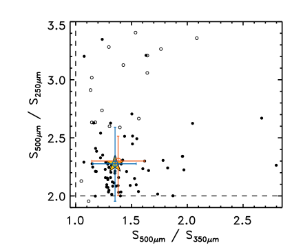
Figure 1: Colour selection ($S_{500\mu{\textrm{m}}}/S_{250\mu{\textrm{m}}}>2$ and $S_{500\mu{\textrm{m}}}/S_{350\mu{\textrm{m}}}>1$) of the H-ATLAS targets observed with AzTEC: filled black circles identified in the $250\mu\textrm{m}$ map and empty circles in the $350\mu\textrm{m}$ (i.e. BANDFLAG 1 and 2 in Ivison et al. (2016), respectively). All targets were detected above $5\sigma$ at $500\mu\textrm{m}$. The yellow star indicates the average colour of the sample, while the blue and orange circles indicate, respectively, the median colour of the targets with and without AzTEC detections above a 4$\sigma$ level. The similar colours shown by the two sub-samples suggest that differences in SEDs cannot explain the bulk of AzTEC non-detections discussed in §3.2.

The final sample of 108 ultra-red Herschel sources selected for LMT follow-up observations has signal-to-noise ratios at 500$\mu$m $\gtrsim 5$ and colour cuts $S_{500\mu{\textrm{m}}}/S_{250\mu{\textrm{m}}}>2$ and $S_{500\mu{\textrm{m}}}/S_{350\mu{\textrm{m}}}>1$ (see Figure 1). Most of the sample ($\sim 80$ per cent) was identified in the $250\mu$m map, with the remaining ones identified in the $350\mu$m residual maps (Figure 1). An additional selection criteria of $35\rm\,mJy<S_{500\mu{\textrm{m}}}<80\rm\,mJy$ was imposed to minimize the contamination by false detections and by gravitationally lensed sources, since the fraction of lensed galaxies falls with decreasing $500\mu{\textrm{m}}$ flux density (with $\sim 100$  per cent of lensed galaxies expected at $S_{500\mu{\textrm{m}}}>100\,$mJy, and $\sim 50$  per cent at $S_{500\mu{\textrm{m}}}>55\,$mJy; Negrello et al. 2010; see also Wardlow et al. 2013; Negrello et al. 2017; Bakx et al. 2020a). The sample was also checked not to have contamination by radio-loud AGN and it was correlated with optical/near-IR imaging (Bourne et al., 2016) to reject nearby galaxies and any obvious lenses that could have entered the sample. Note that, while the contamination by radio-loud AGN is expected to be negligible, that from gravitationally lensed systems is not (e.g. Donevski et al. 2018). This is because the selection of high redshift candidates increases the probability of line of sight alignment with lower redshift massive structures. Indeed, such lensed systems have been confirmed in the sample (e.g. Zavala et al. 2018a).

2.2 AzTEC Observations

Of the 108 targets proposed for the LMT 2014-ES3 campaign (Project 2014AHUGD011, PI: D.H. Hughes), we obtained AzTEC data for 100 sources. AzTEC observations, using the photometry map mode which covers a $\sim 3.5$ arcmin diameter area, were conducted between November 2014 and June 2015 under optimal atmospheric conditions with $\langle{\tau}_{225\rm GHz}\rangle\approx 0.06\pm 0.02$ ($0.03\leq\tau_{225\rm GHz}\leq 0.11$). The integration times devoted to each target were in the range of 3 – 50 min (21.3 hr in total), with a median of 11 min (Table 1). Pointing measurements on known quasars close to the targets were made before and after science observations, and were used in the data reduction process to compensate for any pointing drifts, resulting in a r.m.s pointing accuracy $\lesssim 1$ arcsec.

The data was reduced using MACANA, the C++ version of the standard AzTEC data reduction pipeline (e.g. Scott et al., 2008), with a Wiener-filter applied to improve the detection of point-like sources, at the expense of increasing the nominal FWHM by $\sim 11$  per cent (from $\approx 8.6$ arcsec to $\approx 9.5$ arcsec). The AzTEC pipeline produces four main outputs: signal and signal-to-noise maps, a weight map representative of the noise in each pixel of the map, and a 2D transfer function which tracks the effects of the reduction process on the shape of a synthetic 1 Jy point source (i.e. the Point Spread Function, PSF). Additionally, the pipeline can generate a set of simulated ‘jackknifed’ noise maps by randomly multiplying the clean time-stream data by $\pm 1$. In §3.1 we take advantage of these simulations to measure false-detection-rate (FDR) probabilities in our AzTEC maps.

Table 1: Sample of the 93 H-ATLAS fields targeted at 1.1 mm with AzTEC (Figure 18). Right Ascensions and Declinations (J2000) correspond to the H-ATLAS source centroids where the AzTEC maps were centered. The quoted $\sigma_{\textrm{r.m.s}}$ values correspond to the 85 per cent coverage area of the AzTEC maps (i.e. the $\sim 36.6$ arcsec diameter central area used for our multiplicity analysis).

ID	R.A.	Dec.	$t_{\textrm{int}}$	$\sigma_{\textrm{r.m.s}}$		ID	R.A.	Dec.	$t_{\textrm{int}}$	$\sigma_{\textrm{r.m.s}}$
	[deg.]	[deg.]	[min]	[mJy]			[deg.]	[deg.]	[min]	[mJy]
G09-12469	$140.422082$	$0.895139$	30	$1.15$		NGP-203484a	$204.917078$	$31.369083$	22	$1.49$
G09-44907	$129.345002$	$1.429361$	20	$0.98$		NGP-211862	$193.669996$	$26.823668$	11	$1.62$
G09-58643	$127.822924$	$1.282944$	15	$1.20$		NGP-222757	$199.172916$	$23.675194$	11	$1.35$
G09-62610	$137.354579$	$1.928361$	30	$0.72$		NGP-235542	$195.640411$	$26.673582$	11	$1.78$
G09-64894	$138.189998$	$1.195028$	30	$1.27$		NGP-240219	$192.798743$	$30.998196$	3	$2.67$
G09-71054	$137.194161$	$1.891806$	11	$0.89$		NGP-244082	$199.487500$	$34.490723$	11	$1.73$
G09-75817	$130.181251$	$1.948556$	11	$1.38$		NGP-246114a	$205.309166$	$33.992964$	10	$1.64$
G09-80523	$132.810001$	$1.034833$	15	$1.16$		NGP-248192	$193.215837$	$34.549946$	11	$1.55$
G09-81106a	$132.404541$	$0.248816$	45	$0.82$		NGP-248712	$197.039995$	$22.836945$	11	$1.37$
G09-83808a	$135.189171$	$0.690306$	11	$0.89$		NGP-248948	$192.160006$	$29.628666$	3	$2.78$
G12-23831	$179.638753$	$-1.823000$	15	$1.40$		NGP-249138	$193.611245$	$24.625444$	3	$2.06$
G12-26926a	$183.489161$	$-1.372833$	11	$1.68$		NGP-249475	$206.234994$	$31.441082$	22	$1.55$
G12-31529	$181.649580$	$1.549667$	60	$1.00$		NGP-284357a	$203.214926$	$33.394179$	10	$1.54$
G12-42911	$175.811248$	$0.479556$	10	$1.60$		NGP-49609	$203.213339$	$32.936916$	3	$2.48$
G12-47416	$182.763333$	$0.215972$	22	$1.12$		NGP-55628	$206.604581$	$34.270832$	22	$1.54$
G12-49632	$179.715414$	$-0.164528$	22	$1.17$		NGP-78659	$207.216253$	$26.899221$	6	$2.26$
G12-53832	$184.296255$	$-0.128139$	3	$2.79$		NGP-87226	$205.289998$	$32.933891$	6	$2.59$
G12-58719	$185.308757$	$0.930917$	11	$1.41$		NGP-94843	$204.695005$	$25.669167$	22	$1.44$
G12-73303	$183.509173$	$-1.932833$	11	$1.26$		SGP-101187	$16.970000$	$-30.297194$	11	$1.13$
G12-77419	$182.271252$	$-1.089417$	6	$1.67$		SGP-106123	$13.851250$	$-28.010111$	26	$0.99$
G12-78868	$179.059167$	$1.651611$	3	$2.61$		SGP-211713	$22.584168$	$-31.662361$	15	$1.98$
G15-23358	$214.860005$	$0.193861$	11	$1.11$		SGP-215925	$351.983328$	$-32.768387$	11	$2.38$
G15-26675	$221.138749$	$0.277694$	6	$1.86$		SGP-238944	$0.077917$	$-33.636837$	11	$2.86$
G15-29728	$211.117501$	$1.582861$	11	$1.10$		SGP-267200	$350.531673$	$-34.577248$	11	$1.73$
G15-48916	$214.615831$	$0.789056$	11	$1.12$		SGP-272197	$1.531667$	$-32.444195$	15	$1.62$
G15-57401	$214.029579$	$1.159361$	11	$1.18$		SGP-280787	$350.393744$	$-33.081249$	11	$1.99$
G15-63483	$221.295834$	$0.017833$	11	$1.43$		SGP-284969	$15.858334$	$-30.059082$	26	$0.91$
G15-68998	$222.726660$	$-0.595778$	11	$1.27$		SGP-289463	$25.536667$	$-32.574276$	15	$2.07$
G15-72333	$217.463751$	$1.003722$	11	$1.07$		SGP-293180	$18.160833$	$-30.783361$	11	$1.22$
G15-78944	$221.771665$	$1.024111$	11	$1.28$		SGP-316248	$354.393339$	$-34.839191$	11	$1.43$
G15-82597	$220.157919$	$0.801556$	11	$1.31$		SGP-322449	$344.887505$	$-34.446335$	11	$1.34$
G15-82610	$220.729165$	$1.162305$	11	$1.45$		SGP-323041	$18.501250$	$-32.517056$	5	$2.16$
G15-82660	$215.634999$	$0.505694$	11	$1.08$		SGP-340137	$344.271240$	$-33.839111$	11	$1.24$
G15-83272	$213.802500$	$-0.276806$	3	$1.70$		SGP-348040	$350.404987$	$-35.024223$	11	$1.39$
NGP-112775	$204.170423$	$26.266306$	22	$1.38$		SGP-352624	$19.664167$	$-27.638889$	15	$1.47$
NGP-113203	$196.662912$	$28.464140$	22	$1.43$		SGP-359921	$16.919584$	$-28.448500$	11	$1.21$
NGP-115876	$204.650416$	$27.546473$	22	$1.50$		SGP-379994	$11.356249$	$-32.554695$	15	$1.17$
NGP-124539	$195.212088$	$32.776001$	11	$1.67$		SGP-384367	$21.078333$	$-32.980335$	15	$1.13$
NGP-131281	$193.201246$	$34.404278$	18	$1.36$		SGP-396540	$10.270833$	$-28.222473$	11	$1.37$
NGP-139851	$196.441255$	$25.498222$	3	$2.60$		SGP-396663	$12.548333$	$-32.482918$	11	$1.52$
NGP-145039	$194.372921$	$29.280277$	22	$1.32$		SGP-396921	$16.555417$	$-28.231222$	26	$0.95$
NGP-149267	$203.001666$	$26.422222$	22	$1.36$		SGP-396966	$8.878333$	$-31.504917$	15	$1.27$
NGP-157992	$193.517504$	$27.177750$	3	$2.60$		SGP-399383	$20.202917$	$-30.976528$	15	$1.32$
NGP-168019	$205.405412$	$32.476780$	22	$1.59$		SGP-400082	$8.386249$	$-30.080584$	6	$1.39$
NGP-172727	$196.315827$	$25.516083$	3	$2.50$		SGP-403579	$355.064993$	$-30.445110$	6	$1.28$
NGP-176261	$199.242082$	$33.915947$	9	$1.70$		SGP-68123	$341.992092$	$-29.945444$	11	$1.24$
NGP-194548	$203.407087$	$24.261639$	11	$1.32$
aSelected for spectroscopic follow-up with the 3mm RSR (see Table 2).

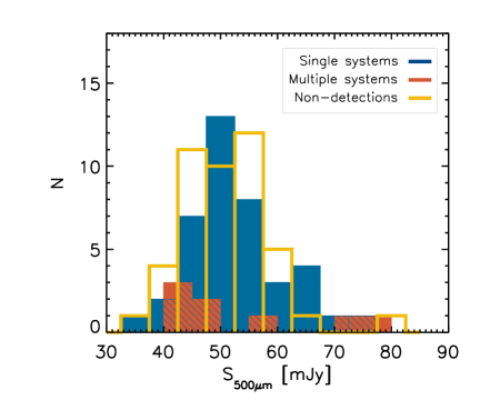
Figure 2: Number of sources as a function of original (before deblending) Herschel $500\rm\,\mu{\textrm{m}}$ flux density. AzTEC sources classified as single and multiple systems (see §3) are illustrated by the blue and orange histograms, while AzTEC non-detections (SNR $<4$) are represented by the yellow histogram. As shown, the three different sets include sources with similar flux densities, discarding possible selection biases in the classification. The bins are slightly shifted for better visualization.

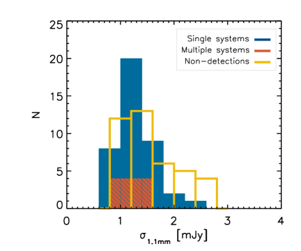
Figure 3: Histogram of achieved sensitivity in the AzTEC observations for the three different classifications: Single systems (in blue), multiple systems (orange), and non-detections (yellow, SNR $<4$). Our survey shows an homogeneous sensitivity, with all of the maps reaching a depth within $0.7<\sigma_{1.1\rm mm}<2.8\,\rm mJy$, therefore ruling out any observational bias in our classification.

Seven of the targets in the SGP field, observed in the poorest weather conditions ($\tau_{225\rm GHz}\approx 0.11$), did not reach the target sensitivity (with $\sigma_{1.1\textrm{mm}}>3.0$ mJy r.m.s.) and, therefore, were removed from the analysis. Thus, we focus on the remaining 93 sources observed with AzTEC (Table 1).

The maps of the final sample have an average depth of $\langle{\sigma}_{1.1\textrm{mm}}\rangle=1.5\pm 0.5\,\textrm{mJy}$ in the central region used for the counterpart analysis (i.e. within the $\sim 85$  per cent coverage area) and $\langle{\sigma}_{1.1\textrm{mm}}\rangle=2.1\pm 0.7\,\textrm{mJy}$ over the 50 per cent coverage area used to detect sources (see §3.1). The filtered maps have PSFs with $\langle{\theta}_{\textrm{FWHM}}\rangle=9.6\pm 0.5\,$ arcsec. Figures 2 and 3 show the $500\,\mu{\textrm{m}}$-flux density distribution of our sample and the attained $\sigma_{1.1\rm mm}\approx 0.7-2.8\,\rm mJy$ r.m.s. distribution of the AzTEC observations respectively.

2.3 RSR observations

Six red-Herschel sources, confirmed with AzTEC to be single systems at high-redshift ($z_{\textrm{phot}}\gtrsim 4$), were selected for spectroscopic follow-up observations with the Redshift Search Receiver on the LMT (Table 2). The RSR is a broadband spectrometer covering the 3 mm window (73-111 GHz) with four detectors in a dual–beam dual–polarization configuration (RSR, Erickson et al., 2007). The observations were done using both the 32m and 50m (since 2018) configurations of the LMT.

The RSR data was reduced using the Dreampy package (Data REduction and Analysis Methods in PYthon, written by G. Narayanan) and following the standard procedure (e.g. Yun et al., 2015; Cybulski et al., 2016; Wong et al., 2017). A careful visual inspection of individual scans was performed to identify and remove those with the noisiest spectral features.

We confirm the redshifts presented in Fudamoto et al. (2017) and Zavala et al. (2018a) for four of these sources, and provide two new determinations at $z=4.768$ and 4.728 (see Table 2). The latter two correspond to G12-26926 and NGP-203484 respectively, whose redshifts are unambiguously identified from at least two emission lines detected with $\textrm{SNR}\geq 5$ in each RSR spectrum. Their redshifts are independently confirmed using the template cross-correlation analysis described by Yun et al. (2015). The same template cross-correlation method yields the unique redshifts of three other objects with two or more emission lines in the RSR spectrum (G09-81106, G09-83808, NGP-284347). Only one emission line is detected in the RSR spectrum of NGP-246114, but it is the same CO(4-3) line at $z=3.847$ previously reported by Fudamoto et al. (2017) who also detected a CO(6-5) transition. Figure 4 shows the identified lines in the RSR spectra. Their fitted parameters are summarized in Table 2. We use these spectroscopic redshifts in Figure 10 to characterize the accuracy of our photometric-redshift determinations.

Table 2: Measured properties of the detected CO transitions in the 3mm RSR spectra. The spectroscopic redshifts estimated in this work from the LMT/RSR spectra are given in column 7 and, for comparison, those previously published are listed in column 8.

ID	Transition	$\nu_{\textrm{line}}$	Peak flux	Integrated flux	FWHM	$z_{\textrm{spec}}$
		[GHz]	[mJy]	[Jy km s-1]	[km s-1]	LMT/RSR	Literature
G09-81106	CO$(4-3)$	$83.40\pm 0.01$	$2.50\pm 0.41$	$1.36\pm 0.17$	$727\pm 128$	$4.531\pm 0.006$	$4.531\pm 0.001^{a}$
	CO$(5-4)$	$104.28\pm 0.02$	$4.06\pm 0.33$	$2.21\pm 0.32$	$899\pm 70$
G09-83808	CO$(5-4)$	$82.03\pm 0.01$	$2.75\pm 0.29$	$1.27\pm 0.17$	$584\pm 120$	$6.026\pm 0.005$	$6.0269\pm 0.0006^{b}$
	CO$(6-5)$	$98.41\pm 0.01$	$2.29\pm 0.41$	$0.90\pm 0.17$	$418\pm 115$
	H2O($2_{11}-2_{02}$)	$106.99\pm 0.01$	$2.96\pm 0.48$	$0.79\pm 0.11$	$227\pm 49$
G12-26926	CO$(4-3)^{d}$	$79.93\pm 0.01$	$8.53\pm 0.45$	$1.98\pm 0.18$	$641\pm 38$	$4.768\pm 0.002^{c}$
	CO$(5-4)^{d}$	$99.86\pm 0.01$	$4.58\pm 0.40$	$0.93\pm 0.22$	$520\pm 41$
NGP-203484	CO$(4-3)$	$80.51\pm 0.01$	$5.39\pm 0.54$	$1.53\pm 0.25$	$376\pm 45$	$4.728\pm 0.002^{c}$
	CO$(5-4)$	$100.59\pm 0.01$	$7.03\pm 0.68$	$1.59\pm 0.17$	$243\pm 31$
NGP-246114	CO$(4-3)$	$95.13\pm 0.03$	$2.05\pm 0.52$	$1.04\pm 0.13$	$476\pm 168$	$3.847\pm 0.002^{e}$	$3.847\pm 0.002^{a}$
NGP-284357	CO$(4-3)^{d}$	$78.16\pm 0.01$	$8.83\pm 0.41$	$1.60\pm 0.21$	$626\pm 36$	$4.891\pm 0.006$	$4.894\pm 0.003^{a}$
	CO$(5-4)$	$97.81\pm 0.01$	$3.31\pm 0.48$	$1.69\pm 0.22$	$535\pm 100$
a Fudamoto et al. (2017). b Zavala et al. (2018a) including an additional [CII] with SMA. c New LMT/RSR determinations derived in this work.
d First published CO transitions using the 50m-LMT. e Estimated including the CO(6-5) transition of Fudamoto et al. (2017).

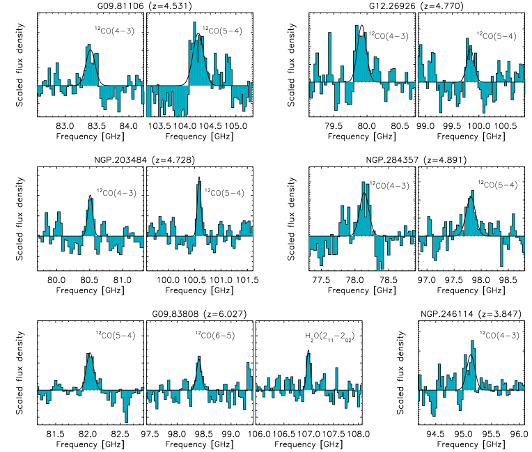
Figure 4: Identified lines in the RSR spectra along with the best-fit Gaussian functions. The redshift of each source is identified on the top and the individual transitions are labeled close to the lines. Each panel has a total width of 6,000 km/s and is centered on the central frequency of the respective line. The identified lines in G09.83808 are the same as in Zavala et al. (2018a). The fitted parameters to each line are listed in Table 2

.

An alternative reduction was produced using a new Python wrapper script developed by D. O. Sánchez-Argüelles for the Dreampy package, known as rsr_driver. This script aims to provide the LMT user community with a front-end interface to generate RSR scientific-quality data from raw observations. The rsr_driver reduction procedure is very similar to the standard process, and below a brief description is presented.

For each detector the RSR backend records the autocorrelation function (ACF) of the observed sky brightness. It is important to notice that the broad 73-111 GHz bandwidth of the RSR is achieved by dividing it into six bands. The raw data is therefore comprised of six ACFs. The pipeline starts by processing the ACFs using a Fourier transform matrix to reconstruct the spectrum of the astronomical source. At this stage, a user defined low order ($\leq 3$) polynomial baseline is computed across each band and subtracted from the spectrum. The relatively fast internal switching ($\simeq 1$ kHz) between the RSR beams allows the minimization of the contribution from atmospheric noise into the ACF; nevertheless, small differences in the switching duty-cycle can introduce large baseline artifacts. To increase the detectability of spectral lines, the rsr_driver can calculate and subtract a Savitzky-Golay filter (SGF) for each band, analogous to performing a high-pass filter on the observed data. The number of points used to simultaneously fit the filter determines its cut-off frequency. In this work we used a length of 55 frequency channels to cut out all the features broader than $\simeq 1.71$ GHz ($\Delta V\simeq 5500$ km/s), which is much larger than the expected CO line widths from high-redshift SMGs. The rsr_driver allows us to automatically remove noisy data from the spectrum. A typical five minutes integration yields a $\sigma_{T_{A^{\ast}}}\simeq 2$ – $4$ mK. All bands with $\sigma_{T_{A^{\ast}}}>5$ mK are therefore ignored by the pipeline. The construction of the final spectrum is achieved by a weighted average of all the observations available for an astronomical source. Figure 5 shows one example of the resulting RSR spectrum and a comparison between the results obtained with the different baseline improvement techniques. It is important to notice that the output of the rsr_driver wrapper produces a significant ($\times 1.5$) improvement on the line-peak SNR of the observed CO transitions, which would be important for the identification of fainter transitions with lower SNRs. This semi-automatic procedure provides an user-friendly tool to reduce RSR data in an homogeneous and efficient way.

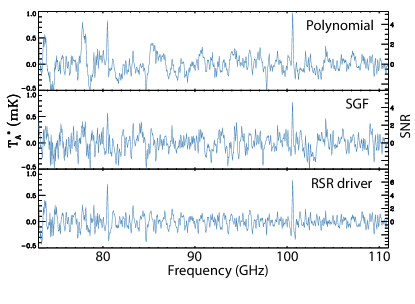
Figure 5: RSR spectra of source NGP-203484 ($z=4.728$) obtained with the different baseline-subtraction techniques available within the pipeline. Top: the standard output of the Dreampy package using a low order polynomial baseline subtraction. Middle: the resulting spectrum by visually inspecting and removing the noisy data, and subtracting a Savistzky-Golay filter (SGF). Bottom: the output produced by the recently developed rsr_driver, including both, a low order polynomial baseline subtraction and a SGF. The output of the rsr_driver wrapper produces a $\sim\times 1.5$ improvement on the line-peak SNR of the observed CO transitions.

3 Analysis and Results

3.1 Source detection and flux measurement

3.1.1 Detection algorithm

Sources were identified using the AzTEC signal-to-noise ratio (SNR) map of each observation and adopting a SNR threshold. If a source is detected in a map, we measure the 1.1 mm flux density and noise at the position of the pixel with the maximum SNR value as well as its celestial coordinates. A mask of 1.5 times the size of the AzTEC beam ($\theta_{1.1\rm mm}\approx 9.5$ arcsec) is applied to the source before repeating the process again until no more sources above our adopted threshold are detected in the map. This process is conducted within the 50 per cent coverage of the maximum depth, which corresponds to typical areas of $6.1-10.8\,\rm arcmin^{2}$ per map.

A $4\sigma$ detection threshold was adopted to minimize the contamination from false detections due to the noise in the maps. False detection probabilities are estimated in three different ways. In method a) the noise simulations generated by the AzTEC pipeline (jackknife maps) are used to identify positive noise peaks (i.e. the false detections), which are then divided by the number of detections in the real maps. In method b), the number of false sources estimated above are divided by the expected number of sources in the map, which we calculate by adding the false sources to the number counts from blank fields (Scott et al., 2012) plus 1 (to compensate for the fact that we are targeting biased fields where we expect to find at least one source). Finally, in method c) the number of negative peaks in the SNR map (representative of the noise in the map) are divided by the number of positive detections.

Figure 6 shows the results of our false detection rate analysis and how, for our adopted search radius of $r=36.6$ arcsec, the three methods converge at $\rm{SNR}\gtrsim 4$, where the contamination due to false detections is $\lesssim 5$  per cent. This contamination drops to $\sim 2$ per cent for $4\sigma$ sources detected within the central and deeper $r=15$ arcsec area of the maps, where the reliability of $3.5\sigma$ and $3\sigma$ detections increases to $\gtrsim$ 90 and 75 per cent respectively.

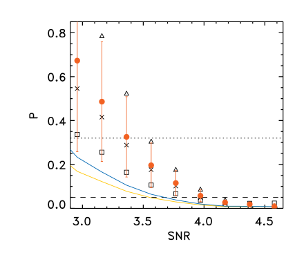
Figure 6: False detection rate (P) estimated within the adopted search area ($r=36.6\,$ arcsec) as a function of signal to noise ratio. Triangles, crosses, and squares correspond to methods a), b), and c), respectively, to estimate the false detection rates (see text). Filled red circles indicate the mean of the three methods. Dashed and dotted lines indicate 5 and 32 per cent contamination, respectively. The blue and yellow curves correspond to the expected false detection rate for sources detected within the deeper central $r=15\,$ and $r=10\,$ arcsec region of the maps.

We have also estimated the completeness of our survey as a function of flux density by inserting synthetic sources (1000 sources per flux density bin) in the AzTEC maps and quantifying the recovery efficiency. The sources are inserted within the 85 per cent coverage region considered in our analysis. Nevertheless, if a source is detected within 5 arcsec from a real detection, it is excluded from the completeness calculation. Figure 7 summarizes the completeness of our survey. Assuming typical SMG SED templates (e.g. Michałowski et al. 2010; da Cunha et al. 2015b; or modified black-bodies with $T_{\textrm{dust}}=40-50\,$K and $\beta=1-2$) at $z\geq 3$, scaled to the average $500\mu\textrm{m}$ flux density of our red-Herschel targets, we infer a completeness $\gtrsim 90$ per cent given the expected 1.1 mm flux densities $\gtrsim 9\,$mJy. Nevertheless, the median flux density of our AzTEC 4$\sigma$ detections of $S_{1.1\textrm{mm}}=7\,\textrm{mJy}$ (see below) suggests a lower completeness of around 75 per cent, which should be considered more reliable.

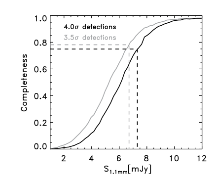
Figure 7: Completeness fraction as a function of 1.1 mm flux density for our AzTEC survey of red-Herschel targets, estimated by inserting synthetic sources in different flux density bins and attempting to recover them above a 4.0$\sigma$ (black) and 3.5$\sigma$ (grey) detection threshold. If we extrapolate the $500\mu\textrm{m}$ flux density using typical SMG SED templates (e.g. Michałowski et al. 2010; da Cunha et al. 2015b; or modified black bodies with $T_{\textrm{dust}}=40-50\,$K and $\beta=1-2$ ) at $z=3$, the expected median 1.1 mm flux densities are $\gtrsim 9\,$mJy, corresponding to a completeness $\gtrsim 90$ per cent. The median flux density of the AzTEC detections, however, suggests a more conservative $\sim 75$ per cent completeness (dashed lines).

The same set of simulations are then used to explore the impact of flux boosting, meaning sources’ flux densities systematically biased upwards by noise and the presence of unresolved astronomical sources below the detection threshold. Given the relatively low number of sources at the depth of our observations (around 0.006 sources per AzTEC beam at our typical $1\sigma$ RMS depth), we infer an average flux boosting factor of $\sim 1.15$ for those sources detected at our detection threshold of SNR=4. The average flux boosting decreases with flux density (or similarly with SNR) and it is almost negligible at SNR$\gtrsim 5.5$. This value is not taken into account given the relatively larger uncertainties of the sources’ flux densities (25 per cent for a source detected at SNR=4).

In the 93 analyzed maps, we find a total of 79 AzTEC detections above our adopted threshold (SNR>4) within the 50 per cent coverage area. The counterpart matching between the Herschel and these AzTEC sources was then performed using the $500\,\mu{\textrm{m}}$ Herschel beamsize as a reference. An AzTEC source is associated with a Herschel source if its AzTEC position lies within $\theta_{500\mu{\textrm{m}}}=36.6\,$arcsec of the Herschel position (although most of them lie within $\sim 15\,$arcsec; see Figure 8). Out of the 93 red-Herschel targets, 40 are associated with individual AzTEC sources, while eight break into multiple AzTEC components (comprising a total of 16 AzTEC detections) and therefore are classified as multiple systems (see §3.3). This leaves 45 Herschel targets with no AzTEC detections at the $>4\sigma$ level, which are discussed in §3.2.

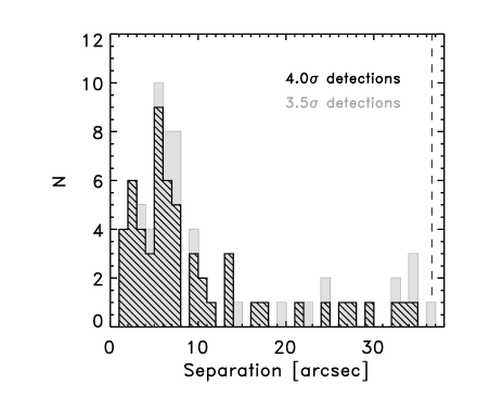
Figure 8: Histogram of the separations between the AzTEC detection and H-ATLAS targeted positions. Although a radius $\theta_{500\mu{\textrm{m}}}=36.6\,$arcsec (vertical dashed line) is used for our counterpart analysis, $\sim 82$  per cent ($75$  per cent) of the $4\sigma$ ($3.5\sigma$) AzTEC sources are separated by $\lesssim 15\,$arcsec off the H-ATLAS target, were the reliability of the detections is $\gtrsim 98\,$ per cent (90 per cent; see Fig. 6).

3.1.2 Serendipitous sources

Additionally, we find 23 AzTEC “serendipitous” detections that lie outside the adopted search radius, i.e. they are not directly associated with any red-Herschel source in the sample and do not contribute to the Herschel-500$\mu$m flux density. Given the total mapped area ($\sim 720$ square arcmin without considering the central regions of the maps) and the flux detection threshold assumed in our analysis ($S_{\rm{1.1mm}}\gtrsim 8$ mJy in the outer region of the maps), the number of serendipitous detections (23) is much larger than the number of sources ($\sim 4$) predicted from AzTEC blank-field number counts (Scott et al., 2012). The probability of finding this number of serendipitous sources within the mapped area by chance is $\sim 8\times 10^{-12}$. Furthermore, moderate resolution single-dish number counts as those reported in Scott et al. (2012) are known to over-estimate the number of bright sources due to source blending (e.g. Lindner et al., 2011; Karim et al., 2013; Béthermin et al., 2017; Stach et al., 2018). Taking this into account would further increase the discrepancy we report.

The estimated overdensity parameter of 4.75 ($\delta(>S)\equiv N(>S)/N(>S)_{\textrm{blankfield}}-1$ = 4.75) is conservative since we are excluding all sources within the multiplicity search radius (i.e. $r=36.6$ arcsec). It is also consistent with the results of Lewis et al. (2018) from LABOCA 870$\mu$m follow-up observations of 22 ultra-red Herschel sources, who found $\delta(>S_{870\mu\textrm{m}})\sim 4-30$ for $S_{870\mu\textrm{m}}\sim 13-16$ mJy (i.e. equivalent to our $4\sigma$ detection threshold of $S_{\rm{1.1mm}}\gtrsim 8$ mJy). This excess suggests that some of these red-Herschel sources are associated with galaxy overdensities. This deserves further analysis which is beyond the scope of this work; therefore, these serendipitous sources are not discussed in the rest of the paper since they are not directly associated with the originally targeted red-Herschel sources.

3.1.3 Deblending Herschel observations

We estimate deblended flux densities in the Herschel bands for all the AzTEC detections in a similar way to that presented in Michałowski et al. (2017, see details of the method therein). Briefly, we extract a square 120 arcsec wide around the position of a given AzTEC source and simultaneously fit 2-dimensional Gaussian functions at the positions of all AzTEC sources within this square patch (the fitting is performed using the IDL mpfit package, Markwardt, 2009). The normalization of each Gaussian function is kept as a free parameter, whereas its FWHM is fixed at the size of the respective Herschel beam. The errors on the deblended flux densities are calculated from the covariance matrix in order to take into account the possible degeneracies in the fitting. This is especially important for close sources that lie within the beam at a given band, whose fluxes are highly degenerate. The confusion limit of the SPIRE data, reported as 5.8, 6.3, and 6.8 mJy beam^-1 at 250, 350 and $500\,\mu\rm m$ (Nguyen et al., 2010), are also added in quadrature. The AzTEC $1.1\,$mm flux densities and the deblended Herschel flux densities derived in this work are reported in Table 3.

3.2 On the nature of non-detections

After performing the counterpart matching, 45 of the 93 analyzed red-Herschel targets do not have an associated AzTEC detection at $\geq 4\sigma$ significance within $36.6$ arcsec. Since the incompleteness of our survey can not explain the bulk of these non-detections (see §3.1), here we explore four possible scenarios to explain them: (1) AzTEC observations do not reach the desired sensitivity; (2) these targets correspond to the faintest Herschel sources and thus deeper observations are needed; (3) these sources are made up of multiple intrinsically fainter components blended within the Herschel beam; and (4) the sources show different SED properties.

As shown in Figure 3, in general, the AzTEC observations on these non-detected targets have a similar r.m.s noise as those in which sources were detected (see yellow histogram in the figure). This confirms the homogeneity of our observations, ruling out the first scenario discussed above. Similarly, these AzTEC non-detections have similar Herschel flux densities to the detected galaxies (Figure 2), spanning a flux density range of $S_{\rm 500\mu m}\approx 40-80\,$mJy. Therefore, if those were single sources with SEDs similar to those of the detected galaxies, we would expect most of them to be detected above the adopted threshold, although a small fraction of them could be associated to the faintest sources. Actually, looking at the AzTEC maps individually, we find 8 (15) sources at SNR $\geq 3.5$ (3.0) close to the Herschel position (at $r\lesssim 10$ arcsec), which are consistent with being single systems but falling below our detection threshold (SNR$=4$). Note that the reliability of these $3.5\sigma$ and $3\sigma$ detections is $\gtrsim 93\,$ and $\gtrsim 80\,$ per cent, respectively (see FDR for the central $r=10\,$arcsec radius region in Fig. 6), which suggest that these single faint sources are real.

Considering that the percentage of spurious detections in the H-ATLAS catalogues is reported to be $\simeq 0.2$  per cent (Valiante et al., 2016), the remaining non-detections are therefore likely multiple systems with individual members’ flux densities below our sensitivity limit or sources with different SED properties. In fact, Valiante et al. (2016) explicitly suggest that “a more important problem than spurious sources is likely to be sources that are actually multiple sources”. After visual inspection, we identify at least nine systems with multiple components at SNR$>3.5$, suggesting that multiplicity is indeed a main reason for the non-detection of these galaxies.

However, although there are no significant differences between the Herschel colours of the detected and the non-detected systems (see Figure 1), suggesting similar SED shapes, we cannot rule out the possibility that some of the non-detected sources have a higher dust emissivity spectral index, $\beta$. This would also decrease the expected flux density in the Rayleigh–Jeans regime probed by the AzTEC 1.1 mm observations, potentially explaining the lack of detections in some of these targets. In fact the median 1.1 mm flux density of the AzTEC detections seems a bit lower than what it is predicted by using typical SED templates (e.g. Michałowski et al. 2010; da Cunha et al. 2015a; see also §3.1). This might be in line with recent results reporting steeper $\beta$ values in $z>3$ galaxies (e.g. Kato et al. 2018; Jin et al. 2019; Casey et al. in prep.), suggesting an evolution of the dust emissivity index with redshift and/or luminosity.

3.3 Multiplicity fraction

Our observations are sensitive to galaxies separated by $\Delta\theta>9.5\,$arcsec. Sources with such separation are hard to detect in the small field of view of interferometric observations as those achieved with ALMA and NOEMA. Indeed, Ma et al. (2019) noted that, for some of their red-Herschel sources, the total flux densities measured by ALMA are systematically lower than those measured with single-dish telescopes, suggesting the presence of multiple components beyond their mapped area. Our observations thus probe multiplicity at a different scale from what has been studied so far with interferometers.

Using our search radius of $36.6$ arcsec (the size of the Herschel beam at $500\mu\textrm{m}$), we find that eight targets from the original sample show source multiplicity, comprising a total of 16 AzTEC detections. This implies that at least $\sim 9$  per cent (8/93) of the red-Herschel targets with AzTEC detections are composed of multiple systems. Additionally, nine of the non-detections are likely multiple systems made of intrinsically fainter galaxies with individual flux densities falling just below our detection threshold (see §3.2). Furthermore, four of the targets originally classified as single detections correspond to multiple systems if the detection threshold is reduced to include $\geq 3.5\sigma$ sources. These additional sources lie within the central ($r\lesssim 15$ arcsec) deeper region of the maps, where the reliability of $3.5\sigma$ detections is $>90$ per cent. Including these, the multiplicity fraction is increased to $\sim 23$  per cent (21/93). An extreme scenario would be if all of the AzTEC non-detections are also assumed to be multiple systems. In that case the multiplicity fraction of the red Herschel sources would be as high as $50$  per cent. Figure 9 shows, for two different search radii, how the multiplicity fraction increases as the detection threshold in our analysis is reduced.

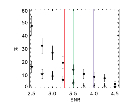
Figure 9: Multiplicity fraction as a function of signal to noise detection threshold, and for 2 search radii: $36.6$ arcsec (circles) and $18.3$ arcsec (stars). Error bars correspond to $\sqrt{N}$. Vertical lines indicate false detection contamination of 5 per cent (dark blue at SNR $\sim 4$), 20 per cent (green at SNR $\sim 3.5$), and 32 per cent (red at SNR $\sim 3.3$), estimated within the central $r=36.6$ arcsec area of the AzTEC maps.

The multiple fraction may be even larger if multiplicity at smaller scales than the AzTEC beam is also present within the sources classified here as single systems.

To probe the multiplicity at smaller scales, we perform two different tests in which the measured PSF profile of single sources is comparable to that of an expected point source. Deviation on the width and shape of the PSF would be expected if two or more sources are blended within the AzTEC beam. First, we derive a radial profile for each detection by azimuthally averaging its flux density and compare its FWHM against that of the point-source PSF. Second, for each AzTEC source, we subtract the point-source PSF scaled to the corresponding measured flux value and quantify the residuals within a $1.5\times\textrm{FWHM}$ area. Then, those sources with broad FWHMs ($\gtrsim 10$  per cent than the ideal PSF – i.e. $\sim 2\sigma_{\textrm{PSF}}$ the standard deviation of the PSFs in our sample) and/or with residuals larger than the noise level are tagged as potential close multiples. Based on this analysis, we expect multiplicity in $21-33$  per cent of the AzTEC detections classified as singles.

These estimations can be compared to the results from interferometric observations on samples of red-Herschel sources. For example, Ma et al. (2019) reported that $\sim 27$ of a compilation of 63 red-Herschel galaxies observed with ALMA, NOEMA and the SMA are close multiple systems. Greenslade et al. (2020) have also recently reported $870\mu\textrm{m}$ and 1.1 mm SMA observation of 34 red $500\mu\rm{m}$-risers from the Herschel Multi-tiered Extragalactic Survey (HerMES, Oliver et al., 2012), and find a $\sim 12$  per cent multiplicity fraction. However, they argue that their 12 non-detections are most likely multiple systems with more than two members, in which case their multiplicity fraction increases to 47 per cent.

Our estimates of the fraction of close multiple systems are in broad agreement with the literature, implying that the multiplicity fraction of the whole sample might be larger than the values reported above when accounting for the multiplicity at smaller scales than the AzTEC beam. Nevertheless, combining these higher-resolution interferometic results with our multiplicity estimations is not straightforward. A careful visual inspection of the 63 red-Herschel sources presented in Ma et al. (2019) indicates that 14 of them ($\sim$ 22 per cent) are multiples at scales below those probed by our AzTEC observations, and would therefore be classified as individual systems in our analysis. This implies that our multiplicity estimates should be increased by an additional $\sim$ 10 per cent due to multiple systems that are not resolved within the AzTEC beam. The resulting total multiplicity fraction of red-Herschel sources would therefore be $\gtrsim 18$  per cent in the conservative scenario and $\sim 60$  per cent in the extreme one, in which most of the non-detections are also considered to be multiples.

Similar results are found if we instead adopt the results from our PSF modelling analysis, but the reader should keep in mind that different factors other than multiplicity (e.g. focus and astigmatism of the telescope, noise gradient in the maps, or even strong gravitational lensing effects) could distort and broaden the shape of the AzTEC beam. Therefore, we stress that follow-up higher angular resolution observations are necessary to derive a robust estimation of the total multiplicity fraction in our sample.

3.4 Redshifts and luminosities

In order to estimate photometric redshifts, luminosities and SFRs, we follow the procedure described in Ivison et al. (2016), in which a library of template SEDs is adopted in order to better characterize the diversity of the intrinsic SEDs and the uncertainties in the derived quantities. We use four SEDs which are representative of dusty star-forming galaxies, and particularly, of red-Herschel sources (see Ivison et al. 2016). This set includes Arp220 (Silva et al. 1998), the Cosmic Eyelash (Swinbank et al. 2010; Ivison et al. 2010), and the two synthesized templates of Pope et al. (2008) and da Cunha et al. (2015b).

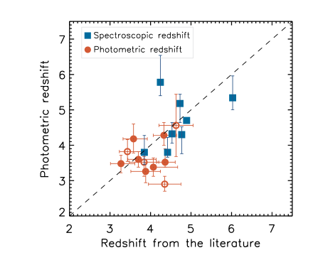
Figure 10: Comparison between the photometric redshifts derived in this work and those reported in the literature (Ivison et al. 2016; Fudamoto et al. 2017; Duivenvoorden et al. 2018; Zavala et al. 2018a; Ma et al. 2019), including both photometric (orange circles) and spectroscopic redshifts (blue squares; see Table 2 and §4.1). The open circles represent sources which are classified as multiple systems based on our AzTEC observations, while all the remaining sources correspond to single systems. In general, our estimated redshifts are in good agreement with those reported in the literature with a mean redshift deviation of $\Delta z/(1+z_{\rm ref})=0.09$ (considering only those sources with spectroscopic redshifts).

Our SED fitting approach is based on a maximum-likelihood method which formally takes into account upper limits in case of non-detections (e.g. Aretxaga et al. 2007; Sawicki 2012). This is important since the Herschel flux densities of some of the sources lie below $2.5\sigma$ after using the AzTEC positions as priors to deblend the Herschel emission (see §3.1). We test our procedure combining the AzTEC photometry (including an additional 5 per cent calibration uncertainty) with all the Herschel data (PACS 100 and $160\,\mu{\textrm{m}}$ and, SPIRE 250, 350, and $500\,\mu{\textrm{m}}$), with only PACS $160\,\mu{\textrm{m}}$ plus all the SPIRE bands, and with only SPIRE photometry. Given the typical low SNR of PACS $100\,\mu{\textrm{m}}$ (plus the possible contribution from emission mechanisms not included in the adopted SED templates – e.g. AGN, PAHs, etc.), the best fits are achieved when using only PACS $160\,\mu{\textrm{m}}$ in combination with the SPIRE and AzTEC photometry. We therefore discard the $100\,\mu{\textrm{m}}$ band during the SED fitting procedure.

For each source in our catalog, a redshift probability distribution is calculated by combining the redshift distributions associated with the four different SED templates described above. Then, the best-fit photometric redshift is assumed to be the one with the maximum likelihood, and the 68 per cent confidence interval is estimated by integrating the combined redshift distribution. As shown in Figure 10, the photometric redshifts derived by this method, which are reported in Table 3, are in good agreement with those reported in the literature (Ivison et al. 2016; Ma et al. 2019; Fudamoto et al. 2017; Zavala et al. 2018a; Duivenvoorden et al. 2018); with eight being spectroscopic redshifts). The relative difference between our redshifts and those derived elsewhere is estimated to be $\Delta z/(1+z_{\rm ref})=0.10$, and 0.09 if only the spectroscopic redshifts are considered. These values are similar to the expected uncertainties for photometric redshifts (Hughes et al., 2002). Additionally, we estimate the photometric redshifts with the MMPZ code (Casey 2020) and find consistent results (with a mean difference of $\Delta z/(1+z_{\rm ref})=0.004$ for the single sources), although with significantly larger uncertainties.

Figure 11 shows the stacked probability redshift distribution of all the AzTEC-detected red-Herschel sources, which has a median redshift of $z_{\rm med}\approx 3.64$. We also plot the stacked redshift distribution of the single and multiple systems separately. Although both distributions have similar median redshifts ($z_{\rm med}\approx 3.8$ vs $3.5$), the multiple systems have a larger fraction of low-redshift sources (27 per cent at $z_{\rm phot}<3$) compared to the single systems (10 per cent). We highlight that, although only $\sim 33$  per cent of the total redshift distribution lie at $z_{\rm phot}>4$, the adopted colour selection criteria is efficient at selecting $z_{\rm phot}>3$ galaxies, where $\sim 85$  per cent of the sample lie. In Figure 11 we also compare the redshift distribution of the AzTEC-Herschel sources with those from similar samples derived in Duivenvoorden et al. (2018) and Ma et al. (2019), which have median photometric redshifts of 3.6 and 3.3, respectively. Similarly, Ivison et al. (2016) reported a median redshift of $3.66$, with $\sim 32$  per cent of the sources lying at $z>4$. Our results are therefore in general agreement with those previously reported.

Figure 11: Normalized redshift distribution of the AzTEC-detected red-Herschel sources derived from the stacking of the redshift probability distribution functions. The components of multiple systems are represented by the orange distribution while the single systems are illustrated by the blue distribution. Although both redshift distributions have a similar median value, that for multiple systems is more skewed towards lower redshifts. The redshift distribution of all the sources is plotted as the black solid curve. For comparison, previous estimations of similar red samples are also included (Duivenvoorden et al. 2018; Ma et al. 2019).

The IR luminosity is then derived using the best-fit template and integrating from $8-1000\,\mu{\textrm{m}}$ (in the rest frame), from which the SFR is estimated assuming the Kennicutt & Evans (2012) calibration for a Chabrier (2003) IMF, SFR [M${}_{\odot}\,{\textrm{yr}}^{-1}$] $=1.48\times 10^{-10}\,L_{IR}\,[L_{\odot}]$. The uncertainties on the infrared luminosities (and hence SFRs) are propagated from the flux density and redshift errors using Monte Carlo simulations. The estimated IR luminosities and SFRs can be found in Table 3.

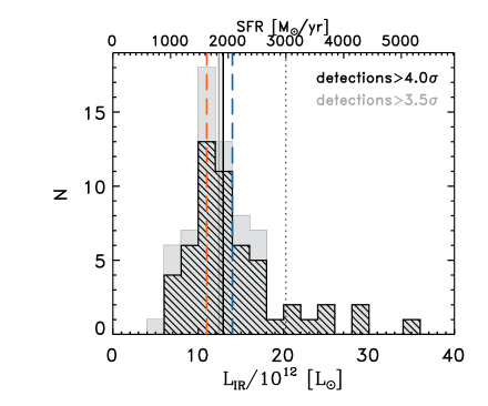
Figure 12: Histogram of IR luminosities and SFRs estimated for the AzTEC detections above $4\sigma$ (black line filled) and $3.5\sigma$ (light grey). The median values of both distributions are indicated with vertical lines, including the median luminosity for the $4\sigma$ single systems ($1.4\times 10^{13}\,L_{\odot}$; dashed blue) and the components of the multiple systems ($1.1\times 10^{13}\,L_{\odot}$; dashed orange). Eight sources in our sample show $L_{\textrm{IR}}>2\times 10^{13}L_{\odot}$ and SFRs $>3000$ M${}_{\odot}\,{\textrm{yr}}^{-1}$ (dotted vertical line), representing a population of extreme star-forming galaxies that cannot be explained within current physically plausible models, unless gravitational lensing effects are included.

Figure 12 shows the IR luminosity and SFR histogram of our AzTEC sources, which have apparent IR luminosities in the range of $12.8\leq\textrm{log}_{10}(L_{\textrm{IR}}/L_{\odot})\leq 13.5$, with a median luminosity of $1.4\times 10^{13}\,L_{\odot}$ for the single systems and $1.1\times 10^{13}\,L_{\odot}$ for the components of the multiple systems. Their SFRs span $\sim 900$ M${}_{\odot}\,{\textrm{yr}}^{-1}$to 5000 M${}_{\odot}\,{\textrm{yr}}^{-1}$, representing some of the most extreme star-forming galaxies known (in the absence of gravitational lensing). These values are in good agreement with those reported in the literature for similar samples. For example, Ivison et al. (2016) reported apparent luminosities in the range of $5\times 10^{12}-6\times 10^{13}\,L_{\odot}$ with a median of $1.3\times 10^{13}\,L_{\odot}$, Ma et al. (2019) derived a median luminosity of $9.0\times 10^{12}\,L_{\odot}$, and Greenslade et al. (2020) report luminosities in the range of $2\times 10^{13}-6\times 10^{13}\,L_{\odot}$. These values are also comparable to those estimated for the sample of DSFGs selected with the SPT, which have a median intrinsic luminosity of $L_{\rm IR}\approx 1.5\times 10^{13}\,L_{\odot}$ (Reuter et al. 2020).

4 Identification of interesting sub-samples

4.1 High-redshift galaxy candidates

To isolate the most promising high-redshift galaxies, we select all those Herschel-AzTEC systems detected above the $4\sigma$ threshold and with $z_{\rm phot}>4$. The 18 sources which satisfy this criterion are indentified in Table 3, three of which are members of multiple systems. Their photometric redshifts span $z=4.0$ to $\sim 5.8$ and have SFRs in the range of $\approx 1000-5000$ M${}_{\odot}\,{\textrm{yr}}^{-1}$, representing some of the most luminous DSFGs known so far (in the absence of gravitational amplification).

Six of these candidates have already been spectroscopically confirmed at $z>4$: SGP-272197 at $z=4.24$ (source SGP-261206 in Fudamoto et al. 2017) and five of the sources in Table 2. Interestingly, G09-838083 ($z=6.03$) was found to be gravitationally lensed by a foreground elliptical galaxy, with a magnification factor of $\approx 9.3$ (Zavala et al. 2018a). This implies that, although the sources were selected to be preferentially non-lensed (see §2), there might be other amplified galaxies in the sample, and therefore, the SFRs quoted above would represent upper limits.

Regardless of their potential gravitational lensing amplification, these sources are ideal targets for future spectroscopic surveys aimed at identifying and characterizing dusty starburst galaxies in the early Universe.

Ivison et al. (2016) developed robust simulations to estimate the different completeness factors affecting the selection of the ultrared Herschel sample. Given the similar selection criteria between samples, we update their completeness estimates considering the 500$\mu$m flux density limit of our sample ($S_{500\mu\textrm{m}}\gtrsim 35$ mJy) and the number of sources in our analysis (93). Using this completeness correction, and considering the number of $z_{\rm phot}>4$ from our analysis, we estimate a lower limit for the space density of $4<z<6$ red DSFGs of $\approx 3\times 10^{-7}\textrm{Mpc}^{-3}$. This is a factor of two lower than that found by Ivison et al. (2016). However, Ivison et al. assumed a SNR detection threshold $\geq 2.5$ for their SCUBA-2/LABOCA observations (FWHM $\sim 18.4$ arcsec), and did not consider potential multiplicity effects.

Combining our estimated space density and the median SFR of our $z_{\rm phot}>4$ sample ($\sim 2500\,\textrm{M}_{\odot}\textrm{yr}^{-1}$ not corrected for potential gravitational lensing effects), we conclude that luminous red Herschel sources contribute $\gtrsim 8\times 10^{-4}\,\textrm{M}_{\odot}\textrm{yr}^{-1}\textrm{Mpc}^{-3}$ to the obscured star formation at $4<z<6$. This value is in very good agreement with the recent estimations of the dust-obscured star formation rate density presented by Zavala et al. (2021) based on ALMA number counts at 1.2 mm, 2 mm, and 3 mm. Their model predicts a dust-obscured star formation rate density of $\approx 10^{+5}_{-6}\times 10^{-4}\,\textrm{M}_{\odot}\textrm{yr}^{-1}\textrm{Mpc}^{-3}$ at $z=5$ from galaxies with IR luminosities in the range of our sources ($12.8\leq\textrm{log}_{10}(L_{\textrm{IR}}/L_{\odot})\leq 13.5$).

4.2 Physically Interacting galaxies

With redshifts in hand, we can speculate the nature of the multiple systems in our sample. Are they chance projections at different redshifts (e.g. Zavala et al. 2015) or physically interacting galaxies (e.g. Oteo et al. 2016)? Examples of both systems have been reported in the literature and, indeed, it is likely that these multiple systems are composed by both physically associated galaxies and chance projections (e.g. Wardlow et al. 2018; Hayward et al. 2018; Stach et al. 2018).

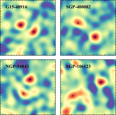
Figure 13: $\rm 76\,arcsec\times 76\,arcsec$ AzTEC 1.1 mm SNR maps of the four most likely physically interacting galaxy candidates in the sample. All the detected sources fall within $36.6$ arcsec of the original Herschel position (the beamsize at $500\,\mu{\textrm{m}}$) and have individual photometric redshifts in agreement with each other within the error bars. These sources, which are typically missed in intereferometric observations due to their small fields of view, are likely galaxy over-densities and/or pre-coalescence galaxy mergers.

As discussed in §3.3, we are only sensitive to sources separated by $\Delta\theta\gtrsim 9.5$ arcsec (which corresponds to $\Delta\gtrsim 70\,$kpc at $z=4$). This prevents us from detecting late-stage mergers as those already identified by ALMA and the SMA (e.g. Oteo et al. 2016). Nevertheless, our observations enables the detection of pre-coalescence galaxy pairs and proto-cluster structures, whose identification by interferometers with small fields of view like ALMA or NOEMA is rather challenging. Such complexes represent ideal laboratories to study the environmental effects on the star formation activity and to understand the star formation process during the earliest stages of galaxy mergers.

To identify the most promising physically interacting systems, we select those multiple galaxies with photometric redshift consistent with each other within $\Delta z<0.5$, since the typical photometric redshift uncertainty from SED-fitting methods is $\approx 0.2-0.3$ (Table 3; see also Aretxaga et al. 2005). Although this threshold might appear too relaxed, we highlight that the probability of finding a pair of two bright sources ($S_{\rm 1.1mm}\gtrsim 5\,$mJy) by chance line-of-sight alignment is very low since their surface density is estimated to be around $0.01\,\rm arcmin^{-2}$ (Scott et al., 2012).

Out of the eight original targets that show multiplicity, only two fulfill this criterion. Two additional systems are identified if the detection threshold is reduced to $3.5\sigma$. These sources are shown in Figure 13 and are also identified in Table 3. As can be seen in the figure, some of these physically interacting candidates are well resolved into two separated sources. For three of these four systems, their redshifts agree within $\Delta z\lesssim 0.06$.

Although further observations are needed to confirm their nature, they might represent observational evidence of the existence of early-stage (pre-coalescence) mergers within the submillimeter galaxy population since their angular separations ($\approx 20-30$ arcsec or $\approx 150-200\,$kpc) and their flux ratios (1:2) are in very good agreement with the predictions from simulations (e.g. Narayanan et al. 2010; Hayward et al. 2012).

5 Discussion and Conclusions

As part of the Early Science Phase of the Large Millimeter Telescope, we obtained AzTEC 1.1 mm observations on a sample of 100 red-Herschel sources. Their red far-infrared colours ($S_{250\mu\rm m}<S_{350\mu\rm m}<S_{500\mu\rm m}$) and bright flux densities ($S_{500\mu\rm m}\approx 35-80\,\rm mJy$) suggest that they are high star formation rate galaxies ($\rm SFRs\gtrsim 500\,$ M${}_{\odot}\,{\textrm{yr}}^{-1}$) at high redshifts ($z\gtrsim 3$).

Combining the AzTEC data with our new deblended Herschel photometry, we constrained the multiplicity fraction in the sample and derived photometric redshifts, IR luminosities, and SFRs for all the sources in the catalog. Our main results are discussed below and are also summarized in Figure 14.

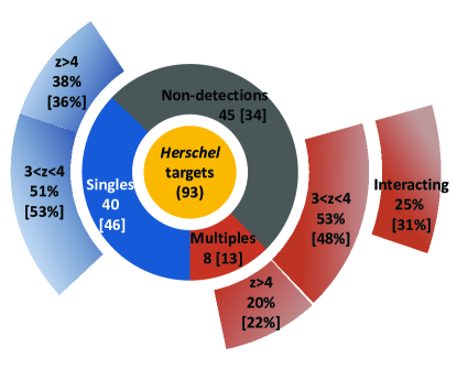
Figure 14: Summary of the results derived from the LMT/AzTEC observations. From the 93 observed red-Herschel targets, and assuming a $4\sigma$ ($3.5\sigma$) AzTEC detection threshold, 40 (46) were associated with single detections, 8 (13) with multiple sources, and 45 (34) with non-detections, within a search radius of $36.6\,$arcsec. These non-detected galaxies are also likely multiple systems, although some of them might be explained by having steep Rayleigh-Jeans slopes (see §3.2). From the detected galaxies, around $85$  per cent of all the AzTEC-Herschel sources lie at $z_{\rm phot}>3$, while only $33$  per cent at $z_{\rm phot}>4$. From the 8 (13) multiple systems, $\sim 25$  per cent ($\sim 31$  per cent) are consistent with being physically associated galaxies ($\Delta z_{\rm phot}\lesssim 0.5$), all of them lying at $z_{\rm phot}\gtrsim 3$. The most promising $z>4$ single sources and the physically interacting galaxy candidates are identified in Table 3.

Thanks to the $\theta_{\rm FWHM}\approx 9.5$ arcsec angular resolution provided by the 32 m illuminated surface of the LMT (a factor of 4 better than Herschel at $500\,\mu\rm m$), we found that 8 of the red-Herschel targets break into multiple components (with SNR $\geq 4$), which implies a multiplicity fraction of $\sim 9$  per cent. This value increases to $\sim 23$  per cent if we include those sources with evidence of multiplicity but slightly below our detection threshold (i.e. formally classified as non-detections). The multiplicity fraction can be even higher (up to $\sim 50$  per cent) if some of the non-detected sources were also made of multiple systems (see §3.3). These multiple sources probe a different scale from what has been studied so far with smaller field of view interferometric observations. Hence, the multiplicity fraction quoted above might be larger if multiplicity at smaller scales (e.g. Ma et al., 2019; Greenslade et al., 2020) is also present within the sources classified here as single systems.

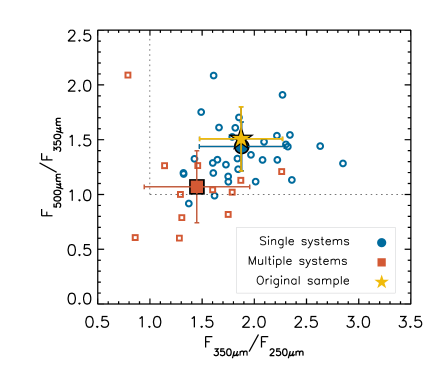
Figure 15: FIR colour-colour plot showing the singles (blue empty circles) and the components of multiple systems (orange empty squares) after deblending the Herschel fluxes using the detected AzTEC positions as priors. The solid blue circle and orange square indicate the average value of the corresponding samples, which have slightly different colours, with the multiple systems showing the least “red” colours. Those sources with upper limits in any of the three bands are not plotted. For comparison, the average colour of the whole sample before deblending the fluxes is marked with a yellow star.

Such high multiplicity should be taken into account when comparing the properties of these galaxies to results from theoretical models and simulations, particularly since source blending artificially increases the redness of the colour in the Herschel bands due to the larger beamsizes of the redder filters. This can be seen in Figure 15, where the FIR colours of the single and multiple systems are plotted after deblending the Herschel flux densities (blue circles and orange squares, respectively), along with the average colour of the whole sample before deblending the fluxes (yellow star). In general, the multiple systems have individual colours which are less red than those of the single systems and the average original colour used for the selection of these galaxies. Indeed, as seen in Table 3, 14 of the 56 AzTEC detections associated with Herschel sources ($\sim 25$  per cent) do not fulfill the condition $F_{250\rm\mu m}<F_{350\rm\mu m}<F_{500\rm\mu m}$ after the deblending of the Herschel fluxes, and 23 ($\sim 41$  per cent) would be excluded after our colour cut ($S_{500\rm\mu m}/S_{250\rm\mu m}>2$ and $S_{500\rm\mu m}/S_{350\rm\mu m}>1$; see §2). This is in line with Ma et al. (2019), who suggest that $\sim 20$  per cent of their sources would not pass the selection criteria of $500\,\mu\rm m$-risers without blending, although lower than the $\sim 60$  per cent derived by Duivenvoorden et al. (2018) from mock observations using the Béthermin et al. (2017) models (note that their sources are brighter with a flux density cut of $S_{500\mu\rm{m}}>63\,$mJy).

Figure 16 shows the distribution of flux density ratios between the brightest component of the multiple system with respect to the total flux density of the system. Our analysis indicates that the brightest component contributes 50 - 75  per cent (with a median $\approx 55$  per cent) at 1.1mm. This is in agreement with results from previous works, using both interferometric and single-dish observations (e.g. Donevski et al., 2018; Ma et al., 2019; Greenslade et al., 2020).

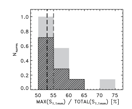
Figure 16: Normalized distribution of the AzTEC 1.1mm flux density ratio between the brightest source of the multiple systems with respect to the total flux density of the system. Solid-gray and line-filled histograms correspond to a $3.5\sigma_{\textrm{1.1mm}}$ and $4.0\sigma_{\textrm{1.1mm}}$ detection thresholds, respectively. Vertical dashed lines indicate the median value for each distribution. Histograms have been normalized to the peak value of the $3.5\sigma_{\textrm{1.1mm}}$ distribution.

To shed light on the multiplicity as a function of the original $500\mu\textrm{m}$ flux density (i.e. before deblending) and to compare to model predictions and other studies, we have divided our sample in two flux density bins: fainter and brighter than $S_{500\mu\textrm{m}}=60$ mJy. Figure 17 shows the multiplicity fraction as a function of our AzTEC signal-to-noise detection threshold for the whole sample (as in Fig. 9), compared to the faint and bright sub-samples. Of the twelve H-ATLAS sources in our sample with $60\leq S_{500\mu\textrm{m}}\leq 80$ mJy, seven are identified as single systems, two break into multiple components, and three have no detections (assuming a SNR threshold $\geq 4$). This corresponds to a multiplicity fraction of $\sim 17$  per cent , which is a factor of two larger than the multiplicity of the fainter sample. This is in agreement with the SMA results from Greenslade et al. (2020) who found, in a sample of 17 SPIRE $S_{500\mu\textrm{m}}>60$ mJy sources, twelve single systems, three multiples, and two non detections (i.e. a multiplicity fraction $\sim 18$  per cent). We note that, although the sample from Greenslade et al. (2020) includes sources with a wider range of 500$\mu$m flux densities (up to $S_{500\mu\textrm{m}}=160$ mJy), they only find multiple systems or non-detections (that could potentially be associated with multiple systems) in sources with $S_{500\mu\textrm{m}}\leq 82$ mJy. These results seem to disagree with models suggesting that Herschel sources with $S_{500\mu\textrm{m}}>60$ mJy are most likely single galaxies, potentially magnified by gravitational lensing effects (e.g. Béthermin et al., 2017).

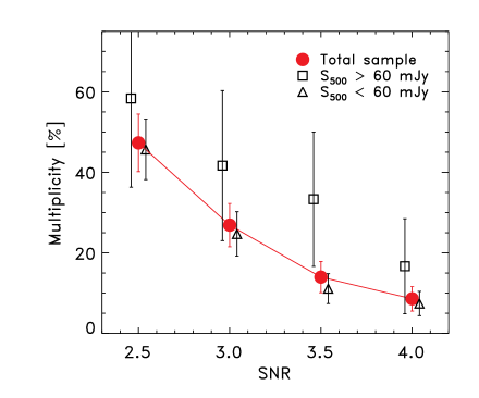
Figure 17: Multiplicity fraction as a function of 1.1mm SNR detection threshold for: the whole sample (red circles), and sources fainter (triangles) and brighter (squares) than $S_{500\mu\textrm{m}}=60$ mJy (before deblending). The multiplicity fraction of the bright sample is $\sim 2$ times larger than that from the fainter sample, and should be considered by models and simulations that try to explain the bright-end of the 500$\mu$m Herschel population of high-$z$ galaxies.

The redshift distribution of all the Herschel-AzTEC sources (singles and multiples) shows that $\sim 33$  per cent of the objects lie at $z_{\rm phot}>4$ and $\sim 85$  per cent at $z_{\rm phot}>3$, with a median redshift of $z_{\rm med}\approx 3.64$ (see Figure 11). These sources show high SFRs in the range of $\approx 900-5000$ M${}_{\odot}\,{\textrm{yr}}^{-1}$(in the absence of gravitational lensing). All of this confirms the high efficiency of the colour selection criterion to select luminous high-redshift ($z>3$) galaxies from the Herschel catalogs.

In §4, we identified the most promising high redshift galaxies candidates, comprising 15 single sources and three members of multiple systems with $z_{\rm phot}>4$. Six of these sources have already been spectroscopically confirmed at $z=4.24-6.03$, including two new spectroscopic redshifts derived in this work using the complete 50 m diameter aperture of the LMT (see §2.3). The rest of the objects comprise ideal targets for future spectroscopic surveys aimed at identifying the most distant dusty star-forming galaxies in the Universe.

Given our $z_{\textrm{phot}}>4$ sample, we estimate a lower limit for the space density of $4<z<6$ red DSFGs of $\approx 3\times 10^{-7}\textrm{Mpc}^{-3}$ which, combined with their median SFR ($\approx 2500\,\textrm{M}_{\odot}\textrm{yr}^{-1}$ not corrected for potential gravitational lensing effects), results in a $\gtrsim 8\times 10^{-4}\,\textrm{M}_{\odot}\textrm{yr}^{-1}\textrm{Mpc}^{-3}$ contribution to the obscured star formation of the Universe at these early epochs (1.5 - 0.9 Gyr after the Big Bang).

Similarly, we identified those multiple systems which could potentially be physically associated (rather than line-of-sight projections). The four candidates, whose members have consistent redshifts with each others within the error bars, are shown in Figure 13. As discussed in §4, these sources might trace galaxy over-densities as those recently discovered within similar samples (e.g. Oteo et al. 2018). Some of them are also in agreement with being galaxy pairs in an early-stage (pre-coalescence) merger as those predicted by simulations (e.g. Hayward et al. 2011). These systems, which given their component separations ($\Delta\gtrsim 20\,$arcsec) are hard to identify with small fields-of-view interferometers, are hence ideal targets to study the environmental effects on the star formation activity and to understand the star formation process during the earliest stages of galaxy mergers.

The catalogue of AzTEC/Herschel sources is given in Table 3, including their updated photometry, derived physical properties, and the best high-$z$ and physically interacting galaxy candidates.

Our results emphasize the importance of accounting for multiplicity in any conclusions derived from Herschel/SPIRE observations, particularly those that estimate number counts or the space density of DSFGs at high redshifts.

The fast mapping speeds of a new generation of large format cameras for the 50m-LMT (Hughes et al., 2020), e.g. MUSCAT (Brien et al., 2018) and TolTEC (Bryan et al., 2018), will result in thousands of DSFGs with better photometry and position accuracy for counterpart identification. The angular resolution provided by the 50m primary mirror of the LMT will allow the identification of multiple systems separated by, at least, angular scales $\gtrsim 5$ arcsec (i.e. $\gtrsim 40$ kpc at $z=3$), and reduce the confusion noise by an order of magnitude ($\sim 0.025$ mJy at 1.1 mm). This would be sufficient to resolve $~{}50$  per cent of the multiple systems identified with interferometers (e.g. Ma et al., 2019) with enough sensitivity to explore the less extreme (and more abundant) population of Luminous Infrared Galaxies ($L_{\textrm{IR}}\gtrsim 10^{11}\textrm{L}_{\odot}$). All of these measurements combined will better constrain the space density of DSFGs and their contribution to the star formation history at the earliest stages of galaxy formation in the Universe.

Data Availability

The datasets generated and analysed during this study are available from the corresponding author on reasonable request.

Appendix A Catalogue and postage stamps

This Appendix presents $\rm 80\,arcsec\times 80\,arcsec$ postage stamps of the 93 H-ATLAS targets included in our analysis (Figure 18), as well as the new photometry of the AzTEC detection (with SNR $\geq 3.5$) and their derived physical parameters Table 3.

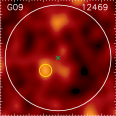
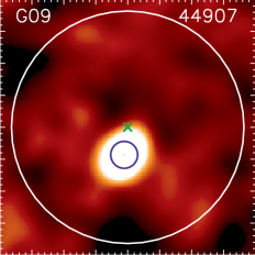
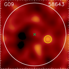
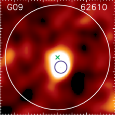
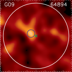
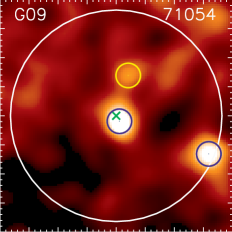
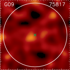
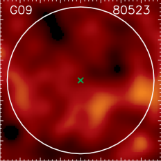
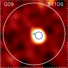
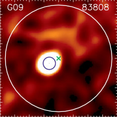
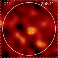
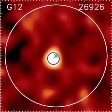
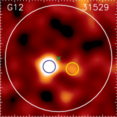
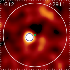
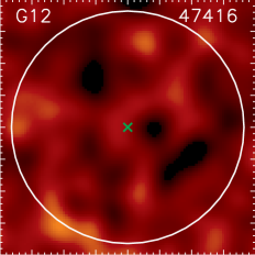
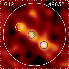
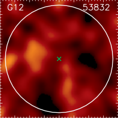
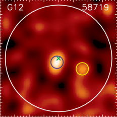
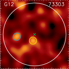
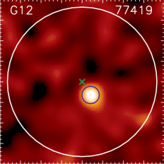
Figure 18: $\rm 80\,arcsec\times 80\,arcsec$ postage stamps of the 93 H-ATLAS targets included in our analysis. Images correspond to the 1.1 mm AzTEC SNR maps. Green crosses and white circles indicate the H-ATLAS targeted position and the adopted search radius ($36.6$ arcsec) respectively. Small circles ($9.5$ arcsec in diameter) mark the position of AzTEC detections, with: yellow corresponding to $3.0\leq\textrm{SNR}<3.5$, light blue to $3.5\leq\textrm{SNR}<4.0$, and dark-blue to $\textrm{SNR}\geq$ 4.0.

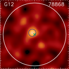
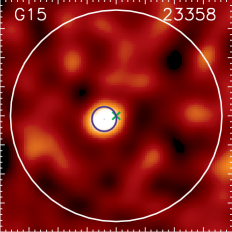
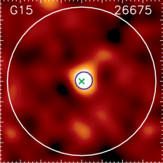
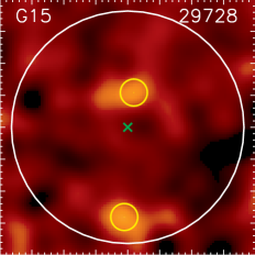
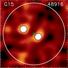
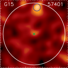
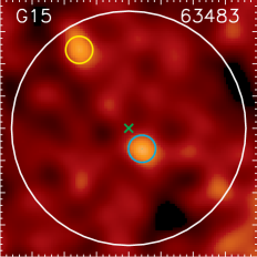
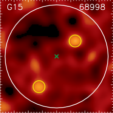
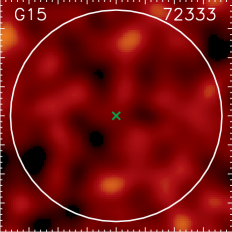
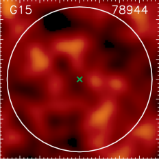
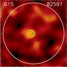
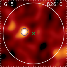
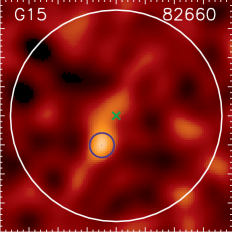
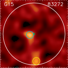
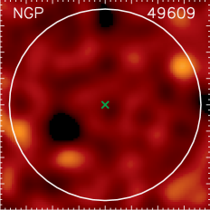
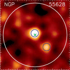
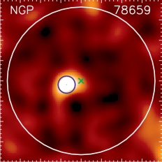
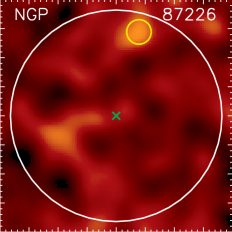
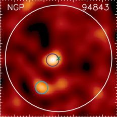
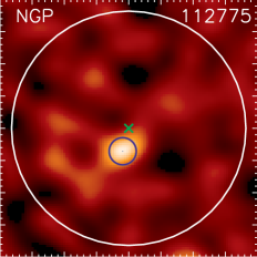
Figure 19: continued

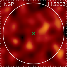
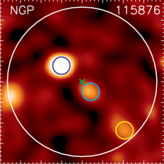
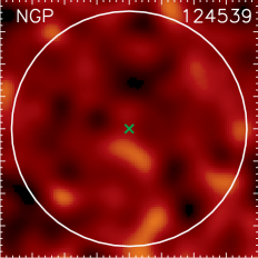
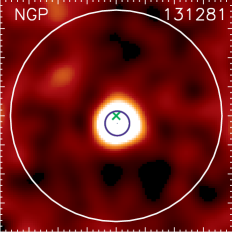
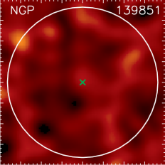
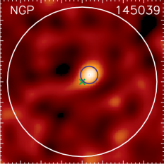
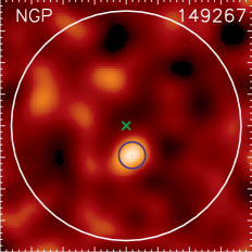
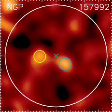
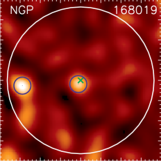
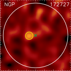
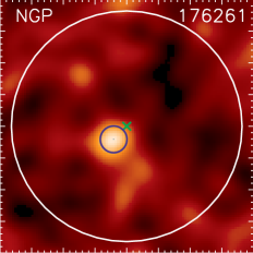
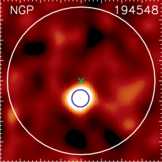
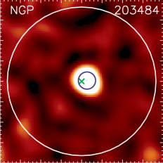
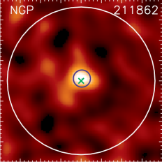
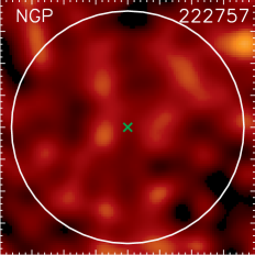
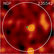
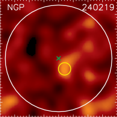
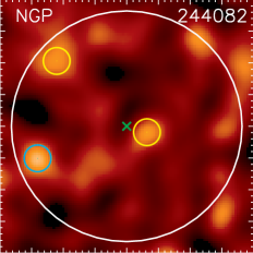
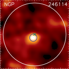
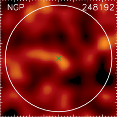
Figure 20: continued

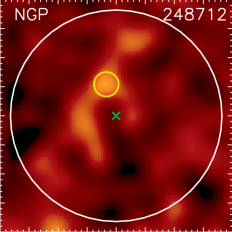
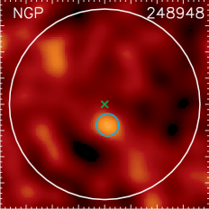
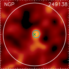
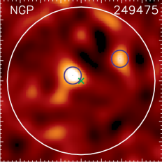
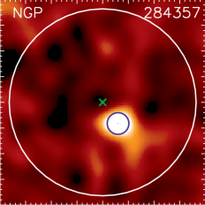
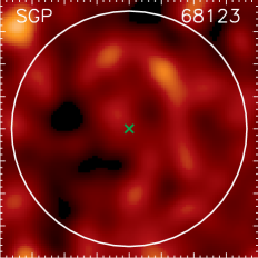
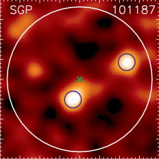
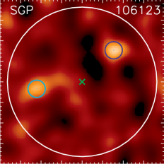
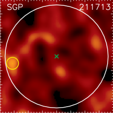
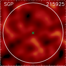
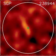
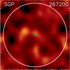
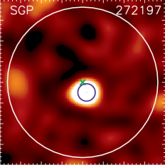
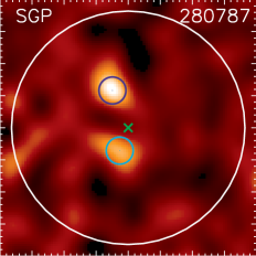
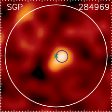
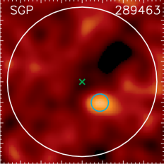
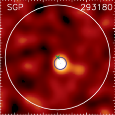
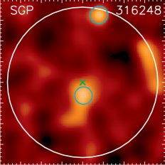
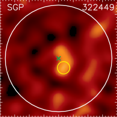
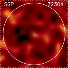
Figure 21: continued

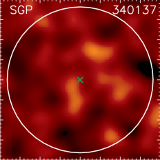
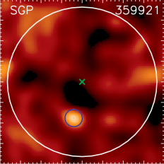
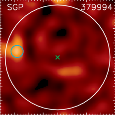
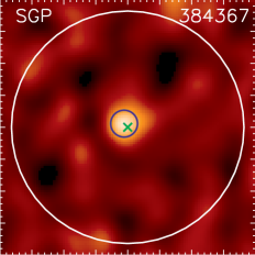
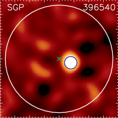
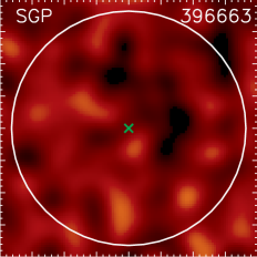
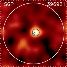
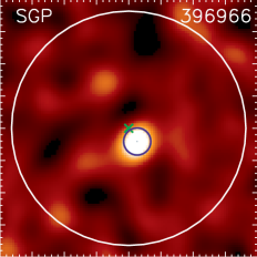
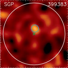
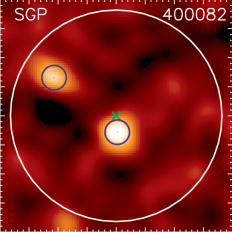
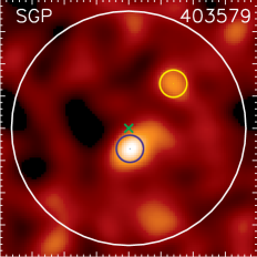
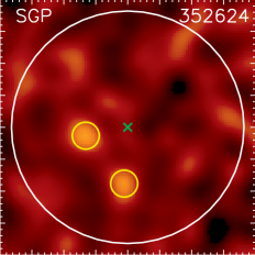
Figure 22: continued

Table 3: AzTEC 1.1 mm detections with SNR $\geq 3.5$, including deblended Herschel/SPIRE flux densities (columns 4-6). The AzTEC flux density and SNR are listed in columns 7 and 8. SED fitted parameters ($z_{\textrm{phot}}$, $L_{\textrm{IR}}$) and SFR are given in columns 9-11 (with dashes indicating that the fitting did not converge). The separation between the AzTEC detection and the Herschel position is given in column 12. The last two columns to the right indicate, for SNR detection thresholds $\geq 4.0$ and $\geq 3.5$, if the source is classified as single (S) or as a member of a multiple system (M). An additional P indicates that the sources are physically interacting system candidates. Our list of robust high-$z$ ($>4$) candidates are indicated with their ID (first column) in boldface font.

ID

R.A.

Dec.

$F_{\rm 250\mu m}$

$F_{\rm 350\mu m}$

$F_{\rm 500\mu m}$

$S_{\rm 1.1mm}$

SNR${}_{\textrm{Az}}$

$z_{\rm phot}$

$L_{\rm IR(8-1000\mu m)}$

SFR

Separation

Class

[deg]

[deg]

[mJy]

[mJy]

[mJy]

[mJy]

[$10^{12}$L⊙]

[M⊙ yr-1]

[arcsec]

$4.0\sigma$

$3.5\sigma$

G09-44907

$129.345104$

$1.427174$

$17.1\pm 7.4$

$37.9\pm 7.8$

$49.8\pm 9.2$

$11.5\pm 0.9$

12.5

$4.14^{+0.28}_{-0.24}$

$17.7^{+5.0}_{-4.0}$

$2614^{+734}_{-586}$

7.9

S

S

G09-62610

$137.353750$

$1.926694$

$17.5\pm 6.7$

$36.6\pm 7.3$

$53.7\pm 8.4$

$8.1\pm 0.7$

11.5

$3.58^{+0.24}_{-0.22}$

$13.5^{+3.5}_{-3.1}$

$2002^{+516}_{-455}$

6.7

S

S

G09-64894

$138.191354$

$1.195965$

$19.9\pm 6.8$

$35.5\pm 7.5$

$55.4\pm 8.0$

$4.8\pm 1.2$

4.1

$3.28^{+0.24}_{-0.24}$

$10.7^{+3.2}_{-2.8}$

$1589^{+472}_{-407}$

5.9

S

S

G09-71054.A

$137.193646$

$1.891493$

$21.0\pm 7.0$

$39.2\pm 7.5$

$44.2\pm 8.9$

$5.4\pm 0.8$

6.6

$3.16^{+0.26}_{-0.22}$

$9.9^{+3.2}_{-2.5}$

$1464^{+468}_{-373}$

2.2

M

M

G09-71054.B

$137.185099$

$1.888368$

$58.9\pm 7.0$

$50.6\pm 7.5$

$30.7\pm 8.9$

$5.6\pm 1.0$

5.6

$2.26^{+0.16}_{-0.28}$

$10.8^{+2.8}_{-3.2}$

$1602^{+411}_{-475}$

34.9

M

M

G09-81106a

$132.403229$

$0.247799$

$14.0\pm 6.0$

$31.0\pm 8.2$

$47.6\pm 8.8$

$11.1\pm 0.8$

13.7

$4.32^{+0.32}_{-0.26}$

$16.8^{+4.9}_{-4.1}$

$2482^{+721}_{-604}$

6.5

S

S

G09-83808a

$135.190729$

$0.689576$

$9.6\pm 7.2$

$21.8\pm 7.4$

$41.6\pm 8.2$

$17.5\pm 0.8$

21.3

$5.34^{+0.62}_{-0.34}$

$24.1^{+8.8}_{-5.5}$

$3566^{+1300}_{-820}$

6.2

S

S

G12-26926a

$183.489479$

$-1.373146$

$26.8\pm 7.0$

$43.1\pm 7.5$

$51.5\pm 8.2$

$14.9\pm 1.6$

9.6

$4.30^{+0.22}_{-0.54}$

$25.9^{+5.6}_{-7.6}$

$3839^{+825}_{-1131}$

1.6

S

S

G12-31529

$181.651146$

$1.548312$

$20.6\pm 7.4$

$36.8\pm 7.9$

$56.1\pm 9.1$

$8.4\pm 0.9$

9.1

$3.64^{+0.22}_{-0.22}$

$14.2^{+3.7}_{-3.2}$

$2096^{+551}_{-467}$

7.5

S

S

G12-42911

$175.812813$

$0.479035$

$18.2\pm 6.9$

$35.8\pm 7.2$

$48.8\pm 8.0$

$13.2\pm 1.5$

8.9

$4.28^{+0.36}_{-0.28}$

$19.8^{+5.5}_{-4.3}$

$2931^{+820}_{-637}$

5.9

S

S

G12-49632.A

$179.712187$

$-0.167757$

$<7.0$

$12.9\pm 7.5$

$<9.5$

$5.2\pm 1.1$

4.7

$-$

$-$

$-$

16.4

M

M

G12-49632.B

$179.716146$

$-0.164424$

$21.7\pm 7.0$

$31.7\pm 7.5$

$40.1\pm 9.5$

$4.6\pm 1.1$

4.3

$3.14^{+0.34}_{-0.32}$

$8.7^{+3.4}_{-2.8}$

$1293^{+500}_{-419}$

2.7

M

M

G12-58719

$185.308854$

$0.930396$

$28.2\pm 7.8$

$45.1\pm 8.1$

$58.1\pm 8.9$

$6.7\pm 1.3$

5.0

$3.26^{+0.26}_{-0.32}$

$13.3^{+3.9}_{-3.7}$

$1971^{+578}_{-544}$

1.9

S

S

G12-73303

$183.514691$

$-1.933354$

$<6.9$

$19.9\pm 7.6$

$34.8\pm 8.6$

$4.1\pm 1.2$

3.5

$3.62^{+0.46}_{-0.62}$

$7.7^{+4.2}_{-3.7}$

$1137^{+614}_{-544}$

10.0

-

S

G12-77419

$182.269896$

$-1.090979$

$13.3\pm 7.9$

$31.2\pm 8.0$

$48.1\pm 9.1$

$8.7\pm 1.6$

5.3

$4.00^{+0.36}_{-0.32}$

$14.6^{+5.1}_{-4.2}$

$2156^{+755}_{-628}$

7.5

S

S

G12-78868

$179.059688$

$1.652340$

$11.9\pm 7.6$

$34.0\pm 7.9$

$43.6\pm 8.5$

$10.1\pm 2.4$

4.2

$4.18^{+0.42}_{-0.40}$

$16.4^{+6.1}_{-5.0}$

$2432^{+899}_{-732}$

3.2

S

S

G15-23358

$214.860938$

$0.193757$

$29.3\pm 6.9$

$51.3\pm 7.4$

$59.7\pm 8.3$

$7.1\pm 1.0$

6.9

$2.94^{+0.36}_{-0.14}$

$11.9^{+2.5}_{-0.9}$

$1758^{+366}_{-137}$

3.4

S

S

G15-26675

$221.138229$

$0.278007$

$23.1\pm 6.9$

$54.6\pm 7.3$

$61.9\pm 7.8$

$11.7\pm 1.8$

6.7

$3.52^{+0.38}_{-0.14}$

$15.9^{+2.8}_{-1.0}$

$2356^{+416}_{-149}$

2.2

S

S

G15-48916.A

$214.619063$

$0.790826$

$15.8\pm 7.0$

$27.7\pm 7.3$

$22.7\pm 8.3$

$6.2\pm 1.1$

5.8

$3.84^{+0.48}_{-0.58}$

$9.6^{+4.7}_{-4.0}$

$1420^{+700}_{-592}$

13.3

MP

MP

G15-48916.B

$214.614271$

$0.788326$

$18.1\pm 7.0$

$23.4\pm 7.3$

$23.4\pm 8.3$

$6.0\pm 1.0$

5.8

$3.50^{+0.64}_{-0.34}$

$10.2^{+6.4}_{-3.5}$

$1508^{+941}_{-521}$

6.2

MP

MP

G15-57401

$214.028437$

$1.168215$

$31.6\pm 6.8$

$43.3\pm 7.6$

$39.7\pm 8.3$

$4.7\pm 1.1$

4.3

$2.84^{+0.26}_{-0.26}$

$9.4^{+3.1}_{-2.5}$

$1387^{+460}_{-375}$

32.1

S

S

G15-63483

$221.294479$

$0.016271$

$19.9\pm 6.8$

$32.9\pm 7.5$

$41.1\pm 8.3$

$5.1\pm 1.4$

3.6

$2.92^{+0.44}_{-0.32}$

$10.4^{+5.0}_{-3.4}$

$1537^{+743}_{-498}$

7.4

-

S

G15-82610

$220.731980$

$1.163035$

$13.0\pm 6.8$

$30.1\pm 7.6$

$43.2\pm 9.0$

$7.2\pm 1.3$

5.3

$3.86^{+0.36}_{-0.32}$

$12.2^{+4.5}_{-3.6}$

$1801^{+668}_{-534}$

10.5

S

S

G15-82660

$215.636146$

$0.503090$

$22.6\pm 7.5$

$52.1\pm 8.1$

$75.9\pm 9.0$

$4.3\pm 1.0$

4.2

$2.68^{+0.42}_{-0.12}$

$10.2^{+2.8}_{-0.8}$

$1507^{+411}_{-112}$

10.2

S

S

G15-83272

$213.803646$

$-0.276910$

$16.3\pm 7.5$

$31.6\pm 7.8$

$54.9\pm 8.8$

$6.7\pm 1.7$

4.0

$3.78^{+0.32}_{-0.30}$

$13.2^{+4.5}_{-3.8}$

$1952^{+671}_{-561}$

4.1

-

S

NGP-112775

$204.170765$

$26.264535$

$25.2\pm 7.2$

$33.3\pm 7.5$

$39.6\pm 8.4$

$6.2\pm 1.3$

4.8

$3.32^{+0.32}_{-0.36}$

$10.8^{+3.7}_{-3.4}$

$1603^{+551}_{-500}$

6.5

S

S

NGP-115876.A

$204.653354$

$27.548868$

$16.6\pm 7.7$

$22.2\pm 8.6$

$15.2\pm 10.9$

$13.8\pm 1.4$

10.0

$5.02^{+1.00}_{-0.62}$

$21.0^{+14.3}_{-8.9}$

$3104^{+2113}_{-1323}$

13.7

S

M

NGP-115876.B

$204.648889$

$27.545326$

$28.1\pm 7.7$

$43.8\pm 8.5$

$50.1\pm 10.4$

$5.0\pm 1.4$

3.6

$2.48^{+0.28}_{-0.30}$

$10.4^{+4.1}_{-3.4}$

$1543^{+610}_{-499}$

6.9

-

M

NGP-131281

$193.200871$

$34.403757$

$26.6\pm 7.6$

$55.3\pm 8.4$

$72.7\pm 9.5$

$19.1\pm 1.3$

15.0

$4.22^{+0.20}_{-0.18}$

$28.8^{+5.4}_{-4.6}$

$4264^{+798}_{-676}$

2.3

S

S

NGP-145039

$194.371603$

$29.281424$

$32.5\pm 7.6$

$42.9\pm 7.9$

$51.4\pm 8.7$

$6.0\pm 1.2$

4.9

$3.08^{+0.22}_{-0.24}$

$11.7^{+3.2}_{-3.0}$

$1736^{+477}_{-442}$

6.3

S

S

NGP-149267

$203.000852$

$26.419826$

$23.2\pm 7.6$

$46.7\pm 7.9$

$52.1\pm 8.4$

$6.2\pm 1.3$

4.7

$3.26^{+0.22}_{-0.22}$

$12.4^{+3.3}_{-2.9}$

$1838^{+486}_{-435}$

9.1

S

S

NGP-157992

$193.515275$

$27.176396$

$22.9\pm 7.6$

$46.2\pm 8.1$

$57.8\pm 8.6$

$9.3\pm 2.5$

3.7

$3.74^{+0.22}_{-0.44}$

$17.9^{+4.4}_{-5.3}$

$2642^{+655}_{-784}$

9.4

-

S

NGP-168019.B

$205.414677$

$32.476257$

$60.3\pm 7.5$

$85.7\pm 8.3$

$82.5\pm 9.3$

$8.2\pm 1.6$

5.2

$2.58^{+0.22}_{-0.14}$

$14.3^{+2.1}_{-1.3}$

$2120^{+312}_{-192}$

33.4

M

M

NGP-168019.A

$205.405540$

$32.476465$

$28.0\pm 7.5$

$50.1\pm 8.2$

$51.2\pm 9.5$

$6.5\pm 1.5$

4.3

$3.20^{+0.26}_{-0.26}$

$12.9^{+3.8}_{-3.3}$

$1912^{+567}_{-486}$

1.2

M

M

NGP-176261

$199.243213$

$33.915007$

$24.3\pm 7.5$

$40.0\pm 7.9$

$52.7\pm 8.7$

$7.3\pm 1.6$

4.7

$3.48^{+0.24}_{-0.26}$

$13.7^{+3.8}_{-3.4}$

$2032^{+567}_{-506}$

5.3

S

S

NGP-194548a

$203.406969$

$24.259451$

$17.9\pm 7.6$

$47.1\pm 8.0$

$67.9\pm 8.7$

$13.8\pm 1.3$

11.1

$3.80^{+0.42}_{-0.14}$

$18.0^{+3.2}_{-1.0}$

$2661^{+474}_{-154}$

7.9

S

S

a Redshifts $>4$ have been spectroscopically confirmed (see Table 2 and §4.1).

Table 4: continued

ID

R.A.

Dec.

$F_{\rm 250\mu m}$

$F_{\rm 350\mu m}$

$F_{\rm 500\mu m}$

$S_{\rm 1.1mm}$

SNR${}_{\textrm{Az}}$

$z_{\rm phot}$

$L_{\rm IR(8-1000\mu m)}$

SFR

Separation

Class

[deg]

[deg]

[mJy]

[mJy]

[mJy]

[mJy]

[$10^{12}$L⊙]

[M⊙ yr-1]

[arcsec]

$4.0\sigma$

$3.5\sigma$

NGP-203484a

$204.915985$

$31.369396$

$20.9\pm 7.7$

$38.5\pm 7.9$

$51.1\pm 9.0$

$21.3\pm 1.4$

15.4

$5.18^{+0.26}_{-0.54}$

$35.0^{+6.9}_{-8.6}$

$5173^{+1023}_{-1268}$

4.1

S

S

NGP-211862

$193.669650$

$26.824187$

$28.2\pm 7.5$

$45.7\pm 8.1$

$45.1\pm 9.1$

$8.1\pm 1.5$

5.4

$3.38^{+0.26}_{-0.26}$

$13.9^{+4.0}_{-3.5}$

$2054^{+595}_{-512}$

2.3

S

S

NGP-244082

$199.496726$

$34.488118$

$<7.6$

$16.2\pm 8.2$

$35.7\pm 9.0$

$6.6\pm 1.7$

3.9

$4.36^{+0.72}_{-0.84}$

$10.6^{+7.3}_{-5.6}$

$1574^{+1074}_{-824}$

34.5

-

S

NGP-246114a

$205.308501$

$33.993556$

$17.3\pm 6.5$

$30.4\pm 8.1$

$33.9\pm 8.5$

$7.8\pm 1.5$

5.2

$3.80^{+0.48}_{-0.34}$

$12.3^{+5.1}_{-3.7}$

$1820^{+754}_{-544}$

3.1

S

S

NGP-248948

$192.159401$

$29.626687$

$9.1\pm 7.8$

$31.3\pm 8.2$

$44.5\pm 8.8$

$9.6\pm 2.7$

3.5

$3.64^{+0.64}_{-0.50}$

$16.6^{+8.5}_{-5.9}$

$2451^{+1254}_{-875}$

7.5

-

S

NGP-249138

$193.610448$

$24.625757$

$21.3\pm 7.6$

$40.5\pm 8.0$

$57.7\pm 8.9$

$7.2\pm 1.9$

3.8

$3.60^{+0.26}_{-0.26}$

$14.8^{+4.2}_{-3.7}$

$2195^{+625}_{-542}$

3.1

-

S

NGP-249475.A

$206.236099$

$31.442021$

$14.8\pm 7.5$

$33.6\pm 8.2$

$40.6\pm 9.8$

$8.4\pm 1.4$

5.8

$3.94^{+0.40}_{-0.34}$

$13.5^{+5.4}_{-4.2}$

$1994^{+792}_{-615}$

5.2

M

M

NGP-249475.B

$206.228529$

$31.444312$

$13.9\pm 7.5$

$12.6\pm 8.2$

$<9.8$

$6.5\pm 1.5$

4.5

$4.62^{+2.12}_{-0.66}$

$9.9^{+19.0}_{-6.9}$

$1471^{+2817}_{-1020}$

26.0

M

M

NGP-284357a

$203.215088$

$33.394556$

$12.6\pm 5.3$

$20.4\pm 7.8$

$42.4\pm 8.3$

$11.1\pm 1.4$

7.7

$4.70^{+0.44}_{-0.36}$

$16.5^{+5.8}_{-4.5}$

$2442^{+859}_{-671}$

11.0

S

S

NGP-55628.A

$206.604457$

$34.271562$

$42.0\pm 8.0$

$47.9\pm 8.4$

$60.5\pm 10.8$

$10.8\pm 1.4$

7.6

$3.52^{+0.16}_{-0.40}$

$20.6^{+4.3}_{-5.8}$

$3055^{+630}_{-853}$

2.7

M

M

NGP-55628.B

$206.599920$

$34.267187$

$46.0\pm 8.0$

$59.0\pm 8.4$

$35.5\pm 10.7$

$6.1\pm 1.5$

4.2

$2.66^{+0.20}_{-0.36}$

$11.1^{+3.2}_{-3.6}$

$1645^{+466}_{-527}$

21.3

M

M

NGP-78659

$207.218236$

$26.898910$

$30.8\pm 7.5$

$53.3\pm 7.9$

$67.8\pm 8.4$

$14.6\pm 2.2$

6.8

$3.90^{+0.24}_{-0.22}$

$23.7^{+5.1}_{-4.4}$

$3506^{+755}_{-649}$

7.2

S

S

NGP-94843.A

$204.696040$

$25.669062$

$33.6\pm 7.7$

$42.3\pm 8.2$

$54.8\pm 10.6$

$6.7\pm 1.4$

5.0

$3.16^{+0.24}_{-0.26}$

$12.5^{+3.7}_{-3.2}$

$1842^{+551}_{-475}$

3.7

S

MP

NGP-94843.B

$204.698351$

$25.663854$

$27.5\pm 7.7$

$31.8\pm 8.2$

$28.5\pm 10.6$

$5.5\pm 1.4$

3.9

$3.22^{+0.30}_{-0.56}$

$10.5^{+4.4}_{-4.4}$

$1554^{+646}_{-651}$

22.6

-

MP

SGP-101187.A

$16.970845$

$-30.299799$

$<7.9$

$35.1\pm 8.1$

$48.6\pm 9.3$

$6.0\pm 1.1$

5.7

$3.48^{+0.30}_{-0.28}$

$10.9^{+4.0}_{-3.2}$

$1611^{+593}_{-470}$

9.7

M

M

SGP-101187.B

$16.962158$

$-30.294590$

$42.7\pm 7.9$

$68.3\pm 8.1$

$71.2\pm 9.3$

$6.1\pm 1.1$

5.3

$2.84^{+0.14}_{-0.20}$

$14.0^{+2.8}_{-3.0}$

$2073^{+415}_{-449}$

29.8

M

M

SGP-106123.A

$13.846177$

$-28.005632$

$<7.9$

$63.5\pm 8.6$

$59.3\pm 9.6$

$4.3\pm 1.0$

4.3

$2.94^{+0.22}_{-0.36}$

$10.5^{+3.2}_{-3.4}$

$1552^{+479}_{-496}$

24.4

S

MP

SGP-106123.B

$13.857975$

$-28.010840$

$<7.9$

$29.8\pm 8.6$

$38.3\pm 9.6$

$3.5\pm 1.0$

3.7

$2.90^{+0.52}_{-0.30}$

$5.8^{+1.8}_{-1.0}$

$860^{+265}_{-143}$

24.4

-

MP

SGP-272197a

$1.530803$

$-32.445340$

$<7.4$

$18.6\pm 8.2$

$46.1\pm 8.6$

$21.1\pm 1.5$

13.8

$5.76^{+0.74}_{-0.40}$

$28.6^{+11.3}_{-7.3}$

$4229^{+1672}_{-1073}$

5.2

S

S

SGP-280787.A

$350.395117$

$-33.077812$

$<7.5$

$11.6\pm 8.1$

$<13.8$

$9.6\pm 1.8$

5.2

$-$

$-$

$-$

13.3

S

M

SGP-280787.B

$350.394372$

$-33.083021$

$<7.5$

$24.2\pm 8.1$

$55.4\pm 8.6$

$7.0\pm 1.9$

3.7

$4.00^{+0.36}_{-0.34}$

$13.8^{+5.0}_{-4.1}$

$2042^{+738}_{-606}$

6.8

-

M

SGP-284969

$15.856769$

$-30.058979$

$<7.8$

$29.5\pm 8.2$

$44.2\pm 9.5$

$4.0\pm 0.8$

4.7

$3.04^{+0.44}_{-0.26}$

$6.3^{+1.5}_{-0.9}$

$929^{+222}_{-128}$

5.7

S

S

SGP-289463

$25.533576$

$-32.576882$

$<7.8$

$27.8\pm 8.5$

$59.0\pm 9.5$

$7.7\pm 2.0$

3.9

$4.00^{+0.34}_{-0.34}$

$14.9^{+5.2}_{-4.5}$

$2202^{+766}_{-667}$

14.6

-

S

SGP-293180

$18.159985$

$-30.784299$

$14.4\pm 7.8$

$23.9\pm 7.8$

$38.5\pm 8.7$

$7.3\pm 1.1$

6.5

$4.02^{+0.42}_{-0.42}$

$11.7^{+4.9}_{-4.1}$

$1734^{+720}_{-607}$

4.6

S

S

SGP-316248.B

$354.390415$

$-34.829924$

$<11.2$

$<11.8$

$<14.4$

$5.8\pm 1.5$

4.0

$-$

$-$

$-$

35.0

-

M

SGP-316248.A

$354.392953$

$-34.840757$

$20.4\pm 7.2$

$24.2\pm 7.6$

$48.5\pm 8.9$

$5.3\pm 1.3$

4.0

$3.48^{+0.34}_{-0.34}$

$10.1^{+3.9}_{-3.2}$

$1501^{+569}_{-472}$

5.8

-

M

SGP-359921

$16.920650$

$-28.453187$

$13.0\pm 8.0$

$24.2\pm 8.5$

$41.2\pm 9.3$

$4.9\pm 1.1$

4.3

$3.32^{+0.60}_{-0.28}$

$7.3^{+2.2}_{-1.0}$

$1072^{+325}_{-143}$

17.3

S

S

SGP-379994

$11.365272$

$-32.553340$

$<7.5$

$18.0\pm 8.2$

$29.9\pm 9.3$

$4.4\pm 1.1$

3.9

$4.00^{+1.14}_{-0.78}$

$7.3^{+8.0}_{-4.3}$

$1078^{+1179}_{-640}$

32.9

-

S

SGP-384367

$21.078458$

$-32.979812$

$<7.6$

$27.0\pm 8.1$

$51.0\pm 9.1$

$4.8\pm 1.0$

4.6

$3.32^{+0.44}_{-0.24}$

$7.3^{+1.6}_{-0.8}$

$1072^{+236}_{-123}$

1.9

S

S

SGP-396540

$10.268114$

$-28.222993$

$9.8\pm 7.5$

$12.8\pm 8.0$

$42.5\pm 8.8$

$9.6\pm 1.3$

7.5

$4.66^{+0.54}_{-0.54}$

$14.3^{+6.8}_{-5.4}$

$2120^{+999}_{-799}$

10.0

S

S

SGP-396921

$16.554353$

$-28.230701$

$<7.6$

$23.2\pm 8.1$

$49.6\pm 9.2$

$4.5\pm 0.9$

5.2

$3.22^{+0.50}_{-0.24}$

$6.9^{+1.8}_{-0.8}$

$1021^{+266}_{-122}$

4.3

S

S

SGP-396966

$8.877234$

$-31.505854$

$20.4\pm 7.8$

$30.5\pm 7.8$

$53.4\pm 8.9$

$8.6\pm 1.2$

6.9

$3.76^{+0.28}_{-0.26}$

$13.9^{+4.2}_{-3.4}$

$2060^{+619}_{-501}$

5.2

S

S

SGP-399383

$20.202309$

$-30.974549$

$24.9\pm 7.7$

$21.3\pm 8.3$

$44.4\pm 8.9$

$4.6\pm 1.3$

3.7

$3.24^{+0.36}_{-0.44}$

$8.9^{+3.9}_{-3.4}$

$1312^{+572}_{-499}$

7.5

-

S

SGP-400082.A

$8.385889$

$-30.081937$

$<7.8$

$20.6\pm 8.5$

$34.2\pm 10.2$

$7.5\pm 1.3$

5.8

$4.56^{+0.88}_{-0.88}$

$11.2^{+8.4}_{-6.0}$

$1658^{+1239}_{-893}$

5.0

MP

MP

SGP-400082.B

$8.392871$

$-30.076729$

$18.1\pm 7.8$

$14.3\pm 8.5$

$29.8\pm 10.2$

$6.6\pm 1.5$

4.4

$4.56^{+1.16}_{-0.92}$

$10.1^{+9.7}_{-5.9}$

$1489^{+1433}_{-876}$

27.6

MP

MP

SGP-403579

$355.064638$

$-30.446674$

$<7.6$

$<8.0$

$32.2\pm 8.5$

$6.1\pm 1.2$

5.2

$4.30^{+0.76}_{-0.84}$

$9.5^{+6.9}_{-5.1}$

$1412^{+1023}_{-756}$

5.8

S

S

a Redshifts $>4$ have been spectroscopically confirmed (see Table 2 and §4.1).

References

- Aretxaga et al. (2003) Aretxaga I., Hughes D. H., Chapin E. L., Gaztañaga E., Dunlop J. S., Ivison R. J., 2003, MNRAS, 342, 759
- Aretxaga et al. (2005) Aretxaga I., Hughes D. H., Dunlop J. S., 2005, MNRAS, 358, 1240
- Aretxaga et al. (2007) Aretxaga I., et al., 2007, MNRAS, 379, 1571
- Asboth et al. (2016) Asboth V., et al., 2016, MNRAS, 462, 1989
- Bakx et al. (2020a) Bakx T. J. L. C., Eales S., Amvrosiadis A., 2020a, MNRAS,
- Bakx et al. (2020b) Bakx T. J. L. C., et al., 2020b, MNRAS, 496, 2372
- Barger et al. (1998) Barger A. J., Cowie L. L., Sanders D. B., Fulton E., Taniguchi Y., Sato Y., Kawara K., Okuda H., 1998, Nature, 394, 248
- Béthermin et al. (2017) Béthermin M., et al., 2017, A&A, 607, A89
- Bothwell et al. (2010) Bothwell M. S., et al., 2010, MNRAS, 405, 219
- Bourne et al. (2016) Bourne N., et al., 2016, MNRAS, 462, 1714
- Brien et al. (2018) Brien T. L. R., et al., 2018, in Proc. SPIE. p. 107080M (arXiv:1807.08637), doi:10.1117/12.2313697
- Brisbin et al. (2017) Brisbin D., et al., 2017, A&A, 608, A15
- Bryan et al. (2018) Bryan S., et al., 2018, in Proc. SPIE. p. 107080J (arXiv:1807.00097), doi:10.1117/12.2314130
- Casey (2020) Casey C. M., 2020, ApJ, 900, 68
- Casey et al. (2014) Casey C. M., Narayanan D., Cooray A., 2014, Phys. Rep., 541, 45
- Chabrier (2003) Chabrier G., 2003, PASP, 115, 763
- Chapman et al. (2005) Chapman S. C., Blain A. W., Smail I., Ivison R. J., 2005, The Astrophysical Journal, 622, 772
- Cox et al. (2011) Cox P., et al., 2011, ApJ, 740, 63
- Cybulski et al. (2016) Cybulski R., et al., 2016, MNRAS, 459, 3287
- Davé et al. (2010) Davé R., Finlator K., Oppenheimer B. D., Fardal M., Katz N., Kereš D., Weinberg D. H., 2010, MNRAS, 404, 1355
- Donevski et al. (2018) Donevski D., et al., 2018, A&A, 614, A33
- Dowell et al. (2014) Dowell C. D., et al., 2014, ApJ, 780, 75
- Dudzevičiūtė et al. (2020) Dudzevičiūtė U., et al., 2020, MNRAS, 494, 3828
- Duivenvoorden et al. (2018) Duivenvoorden S., et al., 2018, MNRAS, 477, 1099
- Eales et al. (2010) Eales S., et al., 2010, PASP, 122, 499
- Engel et al. (2010) Engel H., et al., 2010, ApJ, 724, 233
- Erickson et al. (2007) Erickson N., Narayanan G., Goeller R., Grosslein R., 2007, in Baker A. J., Glenn J., Harris A. I., Mangum J. G., Yun M. S., eds, Astronomical Society of the Pacific Conference Series Vol. 375, From Z-Machines to ALMA: (Sub)Millimeter Spectroscopy of Galaxies. p. 71
- Fudamoto et al. (2017) Fudamoto Y., et al., 2017, MNRAS, 472, 2028
- Greenslade et al. (2020) Greenslade J., Clements D. L., Petitpas G., Asboth V., Conley A., Pérez-Fournon I., Riechers D., 2020, MNRAS,
- Gruppioni et al. (2015) Gruppioni C., et al., 2015, MNRAS, 451, 3419
- Hayward (2013) Hayward C. C., 2013, MNRAS, 432, L85
- Hayward et al. (2011) Hayward C. C., Kereš D., Jonsson P., Narayanan D., Cox T. J., Hernquist L., 2011, ApJ, 743, 159
- Hayward et al. (2012) Hayward C. C., Jonsson P., Kereš D., Magnelli B., Hernquist L., Cox T. J., 2012, MNRAS, 424, 951
- Hayward et al. (2018) Hayward C. C., et al., 2018, MNRAS, 476, 2278
- Hodge & da Cunha (2020) Hodge J. A., da Cunha E., 2020, arXiv e-prints, p. arXiv:2004.00934
- Hughes et al. (1998) Hughes D. H., et al., 1998, Nature, 394, 241
- Hughes et al. (2002) Hughes D. H., et al., 2002, MNRAS, 335, 871
- Hughes et al. (2010) Hughes D. H., et al., 2010, The Large Millimeter Telescope. p. 773312, doi:10.1117/12.857974
- Hughes et al. (2020) Hughes D. H., et al., 2020, in Society of Photo-Optical Instrumentation Engineers (SPIE) Conference Series. p. 1144522, doi:10.1117/12.2561893
- Ivison et al. (2007) Ivison R. J., et al., 2007, MNRAS, 380, 199
- Ivison et al. (2010) Ivison R. J., et al., 2010, A&A, 518, L35
- Ivison et al. (2013) Ivison R. J., et al., 2013, ApJ, 772, 137
- Ivison et al. (2016) Ivison R. J., et al., 2016, ApJ, 832, 78
- Jiménez-Andrade et al. (2020) Jiménez-Andrade E. F., et al., 2020, ApJ, 890, 171
- Jin et al. (2019) Jin S., et al., 2019, ApJ, 887, 144
- Karim et al. (2013) Karim A., et al., 2013, MNRAS, 432, 2
- Kato et al. (2018) Kato Y., et al., 2018, PASJ, 70, L6
- Kennicutt & Evans (2012) Kennicutt R. C., Evans N. J., 2012, ARA&A, 50, 531
- Koprowski et al. (2016) Koprowski M. P., et al., 2016, MNRAS, 458, 4321
- Lacey et al. (2016) Lacey C. G., et al., 2016, MNRAS, 462, 3854
- Lagos et al. (2019) Lagos C. d. P., et al., 2019, MNRAS, 489, 4196
- Lewis et al. (2018) Lewis A. J. R., et al., 2018, ApJ, 862, 96
- Lindner et al. (2011) Lindner R. R., et al., 2011, ApJ, 737, 83
- Ma et al. (2019) Ma J., et al., 2019, ApJS, 244, 30
- Maddox & Dunne (2020) Maddox S. J., Dunne L., 2020, MNRAS, 493, 2363
- Markwardt (2009) Markwardt C. B., 2009, ASPC, 411, 251
- Marrone et al. (2018) Marrone D. P., et al., 2018, Nature, 553, 51
- McAlpine et al. (2019) McAlpine S., et al., 2019, MNRAS, 488, 2440
- Michałowski et al. (2010) Michałowski M., Hjorth J., Watson D., 2010, A&A, 514, A67
- Michałowski et al. (2012) Michałowski M. J., et al., 2012, MNRAS, 426, 1845
- Michałowski et al. (2017) Michałowski M. J., et al., 2017, MNRAS, 469, 492
- Miller et al. (2018) Miller T. B., et al., 2018, Nature, 556, 469
- Narayanan et al. (2010) Narayanan D., Hayward C. C., Cox T. J., Hernquist L., Jonsson P., Younger J. D., Groves B., 2010, MNRAS, 401, 1613
- Narayanan et al. (2015) Narayanan D., et al., 2015, Nature, 525, 496
- Negrello et al. (2010) Negrello M., et al., 2010, Science, 330, 800
- Negrello et al. (2017) Negrello M., et al., 2017, MNRAS, 465, 3558
- Nguyen et al. (2010) Nguyen H. T., et al., 2010, A&A, 518, L5
- Oliver et al. (2012) Oliver S. J., et al., 2012, MNRAS, 424, 1614
- Oteo et al. (2016) Oteo I., et al., 2016, ApJ, 827, 34
- Oteo et al. (2018) Oteo I., et al., 2018, ApJ, 856, 72
- Planck Collaboration et al. (2016) Planck Collaboration et al., 2016, A&A, 594, A13
- Pope & Chary (2010) Pope A., Chary R.-R., 2010, ApJ, 715, L171
- Pope et al. (2008) Pope A., et al., 2008, ApJ, 675, 1171
- Reuter et al. (2020) Reuter C., et al., 2020, ApJ, 902, 78
- Riechers et al. (2013) Riechers D. A., et al., 2013, Nature, 496, 329
- Sawicki (2012) Sawicki M., 2012, PASP, 124, 1208
- Scott et al. (2008) Scott K. S., et al., 2008, MNRAS, 385, 2225
- Scott et al. (2012) Scott K. S., et al., 2012, MNRAS, 423, 575
- Silva et al. (1998) Silva L., Granato G. L., Bressan A., Danese L., 1998, ApJ, 509, 103
- Simpson et al. (2014) Simpson J. M., et al., 2014, ApJ, 788, 125
- Simpson et al. (2020) Simpson J. M., et al., 2020, MNRAS, 495, 3409
- Smail et al. (1997) Smail I., Ivison R. J., Blain A. W., 1997, ApJ, 490, L5
- Stach et al. (2018) Stach S. M., et al., 2018, ApJ, 860, 161
- Strandet et al. (2017) Strandet M. L., et al., 2017, ApJ, 842, L15
- Swinbank et al. (2010) Swinbank A. M., et al., 2010, Nature, 464, 733
- Tacconi et al. (2006) Tacconi L. J., et al., 2006, ApJ, 640, 228
- Toft et al. (2014) Toft S., et al., 2014, ApJ, 782, 68
- Valiante et al. (2016) Valiante E., et al., 2016, MNRAS, 462, 3146
- Vieira et al. (2010) Vieira J. D., et al., 2010, ApJ, 719, 763
- Wardlow et al. (2013) Wardlow J. L., et al., 2013, ApJ, 762, 59
- Wardlow et al. (2018) Wardlow J. L., et al., 2018, MNRAS, 479, 3879
- Wilson et al. (2008) Wilson G. W., et al., 2008, MNRAS, 386, 807
- Wong et al. (2017) Wong O. I., et al., 2017, MNRAS, 466, 574
- Yun et al. (2012) Yun M. S., et al., 2012, MNRAS, 420, 957
- Yun et al. (2015) Yun M. S., et al., 2015, MNRAS, 454, 3485
- Zavala et al. (2015) Zavala J. A., et al., 2015, MNRAS, 452, 1140
- Zavala et al. (2018a) Zavala J. A., et al., 2018a, Nature Astronomy, 2, 56
- Zavala et al. (2018b) Zavala J. A., et al., 2018b, MNRAS, 475, 5585
- Zavala et al. (2021) Zavala J. A., et al., 2021, ApJ, 909, 165
- Zhang et al. (2018) Zhang Z.-Y., Romano D., Ivison R. J., Papadopoulos P. P., Matteucci F., 2018, Nature, 558, 260
- da Cunha et al. (2015a) da Cunha E., et al., 2015a, ApJ, 806, 110
- da Cunha et al. (2015b) da Cunha E., et al., 2015b, ApJ, 806, 110