Bayesian graphical modeling for heterogeneous causal effects
Abstract
Our motivation stems from current medical research aiming at personalized treatment using a molecular-based approach. The broad goal is to develop a more precise and targeted decision making process, relative to traditional treatments based primarily on clinical diagnoses. Specifically, we consider patients affected by Acute Myeloid Leukemia (AML), an hematological cancer characterized by uncontrolled proliferation of hematopoietic stem cells in the bone marrow. Because AML responds poorly to chemoterapeutic treatments, the development of targeted therapies is essential to improve patients’ prospects. In particular, the dataset we analyze contains the levels of proteins involved in cell cycle regulation and linked to the progression of the disease. We analyse treatment effects within a causal framework represented by a Directed Acyclic Graph (DAG) model, whose vertices are the protein levels in the network. A major obstacle in implementing the above program is however represented by individual heterogeneity. We address this issue through a Dirichlet Process (DP) mixture of Gaussian DAG-models where both the graphical structure as well as the allied model parameters are regarded as uncertain. Our procedure determines a clustering structure of the units reflecting the underlying heterogeneity, and produces subject-specific estimates of causal effects based on Bayesian model averaging. With reference to the AML dataset, we identify different effects of protein regulation among individuals; moreover, our method clusters patients into groups that exhibit only mild similarities with traditional categories based on morphological features.
Keywords: Directed acyclic graph; Dirichlet process mixture; Subject-specific graph; Personalized treatment; Tumor heterogeneity.
1 Introduction
1.1 Background and motivation
Heterogeneity of individual responses to treatment is a pervasive aspect in a variety of clinical domains. An example is cancer which is not a single disease as it involves subtypes characterized by distinct sets of molecules; this implies that patients will react differently to the same treatment. Currently the best treatment is identified based on clinical diagnoses as opposed to a molecular-based approach which would allow a more precise and targeted approach to decision making, leading to better treatments and eventually more favorable prognoses. At present there exists a variety of methods to identify cancer subtypes [46, 41]; however they cannot establish whether subtypes show heterogeneous responses toward a treatment. Identifying subtypes with heterogeneous treatment effects is a causal problem that need be addressed for a more informed decision strategy [49].
In this paper we consider a dataset concerning patients affected by Acute Myeloid Leukemia (AML). AML represents an aggressive hematological cancer characterized by uncontrolled proliferation of hematopoietic stem cells in the bone marrow. AML responds very poorly to chemoterapeutic treatments, with a 5-year overall survival rate of about 25%; the development of new targeted treatments therefore represents a key strategy to improve patients’ prospects. In addition, AML is widely heterogeneous with numerous genetic aberrations. Consequently, knowledge facilitating individualization of targeted therapies under development in AML is sorely needed. Several subtypes of AML have been identified mainly on the basis of morphologic features. However, interest has been recently focused on developing improved classification schemes that more accurately explain the AML heterogeneity and in particular its response to therapies.
The dataset analysed here includes protein levels for 256 newly diagnosed AML patients and is provided as a supplement to Kornblau et al. [22]. Because protein function regulates the phenotypic characteristics of cancer, a proteomic-based classification can provide relevant information for pathogenesis and prognosis of patients. In this direction tumor profiling accounting for patients heterogeneity can provide insights on the effect of targeted therapies on individualized basis. We apply our methodology to the AML dataset to investigate the existence of clustering characterized by differential graph structures as well as model parameter configurations. In addition, we evaluate a battery of causal effects on selected proteins in the network whose regulation has been established to play a crucial role in AML progression and response to therapy. We then pair clusters with heterogeneity of causal effects, and identify broad patterns of potential use for targeted therapy.
1.2 Overview of our model
In this subsection we provide the broad picture underlying our model, while leaving technical specifications to later sections. In our setup we have a collection of variables , exemplified by protein expressions in the AML dataset. When we are interested in isolating one of the variables as a response we label it as . We consider a sample of size from the -dimensional population. To account for potential heterogeneity of the subjects we assume that the statistical model is a mixture of Directed Acyclic Graph (DAG) models. This means that, if we knew the mixture component of each sample case, its distributional family would factorize according to the corresponding DAG, equivalently it would be Markov with respect to that DAG. Graphical models [23] are very effective for encoding conditional independencies. In our setting however we view a DAG as a causal model [33]; in particular this means that the joint interventional distribution of the variables, following a hypothetical intervention on a variable in the system, would still be Markov relative to the DAG, save for the component subjected to intervention, which will be specified separately. This stability assumption is crucial to define the notion of total causal effect on following an intervention on [26].
From a modeling perspective, we start by assuming that the joint observational distribution belongs to a Dirichlet Process (DP) mixture of Gaussian DAG models; see Müller & Mitra [28] for an overview of DP mixtures. The mixing measure is over the space of priors on where is a DAG and the parameters of a -variate Normal distribution having precision , where is the space of symmetric and positive-definite matrices constrained by being Markov relative to . We take the baseline measure of the DP as , and specify as a Normal-DAG-Wishart prior after a suitable reparameterization involving a Cholesky-type decomposition of [6]. We employ a constructive procedure which produces a prior under any DAG model based on the elicitation of a single standard Normal-Wishart prior on , with unconstrained. In this way, not only is the elicitation procedure drastically simplified, but the marginal likelihood of DAGs belonging to the same Markov class can be shown to be constant (score equivalence), besides being available in closed form. Computations for our model are performed through an MCMC strategy based on a slice sampler [45] and the Partial Analytic Structure (PAS) algorithm of Godsill [18].
Our contribution can be summarized as follows. We provide a Bayesian modeling framework to evaluate heterogeneous causal effects based exclusively on observational, i.e. non-experimental data. Specifically, our model: i) accounts for individual heterogeneity through an infinite mixture of Directed Acyclic Graphs models; ii) allows for structure (DAG) and parameter uncertainty; iii) determines a clustering structure of the units; iv) produces subject-specific causal effects incorporating uncertainty on various aspects of the model through Bayesian model averaging. When applied to the AML data it highlights that protein regulation produces heterogeneous effects, and identifies cluster of patients potentially benefiting from selective interventions.
1.3 Related work
The literature on the analysis of heterogeneous causal effects has been growing lately, especially in the machine learning community where tree-based methods, in particular random forests, have found natural applications. Works in this area have been carried out mostly within the potential outcome framework [38]; see for instance Athey & Imbens [1], Wager & Athey [44], Lee et al. [24] and Hahn et al. [19] for a Bayesian viewpoint.
A more decision theoretic approach is presented in Shpitser & Sherman [42] who discuss identification of personalized effects in causal pathways. and explore settings where the goal is to map a unit’s characteristics to a treatment tailored to maximize the expected outcome for that unit. This line of approach is also connected to literature spanning from dynamic treatment regime to mediation analysis.
Moving to a Bayesian perspective, inference on causal effects within the causal graph framework has been traditionally carried out assuming a homogeneous population, that is the observations are (conditionally) independent and identically distributed from a zero-mean Gaussian DAG-model; see for instance Castelletti & Consonni [8] and Castelletti & Consonni [7].
So far heterogeneity has been mostly linked to differential Bayesian structural learning as in multiple graphical modeling, where each model is associated to a specific group which is known in advance; see Peterson et al. [35] and Castelletti et al. [9] for directed graphs. Also, Ni et al. [31] provide an extensions to multi-dimensional graphs. A previous important attempt to deal explicitly with heterogeneity using a DP mixture of Gaussian graphical models is Rodríguez et al. [36]. There are however notable differences with respect to our work. First of all they only consider structural and parameter learning for undirected graphs; secondly there is no discussion of causal inference. Bayesian nonparametric techniques have been used in graphical modeling also for robustness purposes: see Finegold & Drton [13, 14], and Cremaschi et al. [10] for an extension to more general measures.
Bayesian nonparametric methods for causal inference have been also employed in a potential outcome framework; see for instance Rubin [39]. In particular, Roy et al. [37] consider marginal structural models to evaluate the causal effect of a treatment on a survival outcome and allow for heterogeneity by implementing a dependent DP for the response given a set of confounders. Moreover, Oganisian et al. [32] implement a DP mixture of zero inflated regression models for pathological data exhibiting excesses of zeros; their method allows for prediction, causal effect estimation and clustering of patients into homogeneous groups sharing the same propensity score distribution.
We close this subsection by pointing to a more foundational line of research that connects invariance, causality and robustness [3] where an important role is played by heterogeneity; the latter however relates to different “environments”, seen and unseen, and thus has a broader scope than the notion of heterogeneity employed in this paper.
1.4 Structure of the paper
The organization of the rest of this paper is as follows. In Section 2 we provide some background results on causal effect estimation based on DAGs. We then introduce in Section 3 our DP mixture of Gaussian DAG models with particular emphasis on the specification of the baseline prior distribution for model parameters. Posterior inference is discussed in Section 4. In Section 5 we conduct extensive simulation experiments to evaluate the proposed method in terms of structural learning, clustering and causal effect estimation. Section 6 is entirely devoted to the analysis of the AML data, highlighting the heterogeneity of causal effects as well as the clustering structure. Finally, Section 7 offers a few points for discussion. Some theoretical results on parameter prior distributions and computational details are reported in the Supplementary material.
2 Background
2.1 Directed acyclic graphs and causal effects
Let be a collection of real-valued continuous random variables with joint p.d.f. . Let also be a Directed Acyclic Graph (DAG), where is a set of nodes associated to variables and is a set of edges. If , then and we say that is a parent of node ; by converse we say that is a child of . The set of all parents of in is then denoted by . Under DAG the joint density factorizes as
| (1) |
Factorization (1) is often called the Markov property and determines conditional independence relations among (set of) nodes which can be read-off from the DAG using graphical criteria. We also assume faithfulness of to which prescribes that the conditional independencies implied by (1) are exactly those graphically encoded by . We remark that faithfulness holds, up to sets of Lebsegue measure zero, under many common families of distributions such as the Gaussian model (Section 2.2).
Consider now a (deterministic) intervention on variable which consists in setting to the value and is denoted as . The post-intervention density is [33]
| (2) |
where, importantly, each term in (2) is the corresponding (pre-intervention) conditional density of Equation (1); this implies that the data generating mechanism is stable under intervention, because the latter only affects the local component distribution which is reduced to a point mass on .
In particular, we are interested in evaluating the causal effect of an intervention on a response variable ; by convention we set . The post-intervention distribution of is then obtained by integrating (2) w.r.t. which simplifies to
| (3) |
if ; on the other hand if then ; see Pearl [33, Theorem 3.2.2]. Equation (3) uses the most common adjustment set, namely the set of parents of ; other valid adjustment sets are however possible; see Witte et al. [47]. Also, it is common to summarize the causal effect on of an intervention on through the derivative of the expected value of (3)
| (4) |
Clearly if belongs to some parametric family indexed by (a parameter specific to the underlying DAG), the causal effect will be a function of ; accordingly, inference on will drive inference on .
2.2 Gaussian DAG models
In the following we focus on Gaussian DAG models and assume
| (5) |
where and , the set of all symmetric positive definite (s.p.d.) precision matrices Markov w.r.t. .
Equation (5) can be alternatively written as a Structural Equation Model (SEM). Given , consider the reparameterization
| (6) |
for , where , , , . Parameters ’s correspond to the non-zero elements of a matrix with all diagonal entries equal to one. Moreover, if we let be a diagonal matrix with -element and , the SEM representation of (5) is given by
where . Equivalently, we can write
| (7) |
where denotes the Normal density of . Equation (7) represents the density of a Gaussian DAG model after the reparameterization ; compare also Equation (1). Finally we note that .
Consider now the causal effect of an intervention on as defined in Equation (4). Under the Gaussian model (5), the post-intervention distribution of can be written as
| (8) |
where each density under the integral sign is a suitable Normal. Taking the expectation of the post-intervention distribution on the left-hand-side of (8), and interchanging the order of integration in the right-hand-side, one obtains
| (9) |
so that, using (4), the causal effect of on is , the coefficient associated to in the conditional expectation of given with . Therefore, the causal effect can be retrieved from the covariance matrix as
| (10) |
where subscript refers to the first element of the vector, having implicitly assumed that variable “” appears first in the set .
3 Dirichlet process mixture of Gaussian DAG models
We consider a Dirichlet Process (DP) mixture of Gaussian DAG models so that
| (11) |
where denotes the density of a Gaussian DAG model defined in (7), and follows a DP with parameters (precision) and (baseline), written . With regard to the baseline measure we set
| (12) |
where priors and will be shortly defined in Section 3.1.
Let now , , be independent draws from (11). Recall that in a DP mixture each sample , , has potentially a distinct parameter . Let be the number of unique values among and a sequence of indicator variables, with , such that . Denote now with the data matrix obtained by row-binding the individual observations ’s. It is instructive to write the DP mixture models in terms of the random partition induced by the ’s,
| (13) |
Representation (13) is easily interpretable. The model groups observations into homogeneous classes, with samples within each class generated from a standard Gaussian DAG model. In practice, for a given partition, is split into sub-matrices , , each collecting all observations such that .
3.1 Prior on DAG parameters
We now detail our choice of prior distributions and .
For a given DAG , let be the corresponding parameters, where , . We first consider the reparameterization introduced in Section 2.2. Our elictation procedure relies on the method of Geiger & Heckerman [16]. A main feature of this approach is that we only need to specify a prior for the parameters of a complete DAG model, , with unconstrained; the prior for any other (incomplete) DAG is then derived automatically, as we detail in the Supplementary material. Additionally, and importantly, this procedure guarantees compatibility of priors in the sense that Markov equivalent DAGs are scored with the same marginal likelihood. Specifically, we show that a proper Normal-Wishart prior, , leads to the compatible prior
| (14) | |||||
where
and .
3.2 Prior on DAG structures
Let be the space of all DAGs on nodes. For a given DAG , let be the 0-1 adjacency matrix of its skeleton, that is the underlying undirected graph obtained after removing the orientation of all its edges. Accordingly, for each -element in , if and only if or , and zero otherwise. Conditionally on a prior probability of inclusion we assume for each . Therefore,
| (15) |
where is the number of edges in (equivalently in its skeleton) and corresponds to the maximum number of edges in a DAG on nodes.
We then proceed hierarchically by assigning . Integrating out , the resulting prior on is
A similar prior was introduced by Scott & Berger [40] for variable selection in linear models, where it was also shown to account for multiplicity correction. Finally, we set
| (16) |
Hyperparameters and can be chosen to reflect a prior knowledge of sparsity in the graph, if available; in the next section we fix for instance , , which is consistent with an expected prior probability of edge inclusion smaller than ; see also Peters & Bühlmann [34]. The default choice , which corresponds to , can be instead adopted in the absence of substantive prior information.
Finally, the prior on the precision parameter is taken to be . Hyperparameters control the prior number of clusters [11]. A sensitivity analysis on a grid of values for and led to the choice (hereafter employed) , which results in a moderate expected number of groups, and a approximate prior credible interval ; see also Murugiah & Sweeting [29] for empirical approaches driving the choice of and .
4 Posterior inference: clustering, structural learning and causal effects
We implement an MCMC algorithm to sample from the posterior distribution of the DP mixture model (11). Our proposal relies on a slice sampler [45] which is based on the number of explicitly represented mixture components and maintains the structure of a blocked Gibbs sampler. Full details are provided in the Supplementary material.
The output of our MCMC scheme is a collection of draws approximately sampled from the (augmented) posterior of where is the triple . Specifically, for each MCMC iteration our algorithm returns the -dimensional vector of individual allocations , with where is the number of distinct clusters, together with the collection of distinct cluster-specific parameters From the MCMC output we can construct an posterior similarity matrix whose -element represents the posterior probability that subjects and belong to the same cluster, namely
| (17) |
The latter can be used to obtain an estimate of the partition induced by the DP, e.g. by including subject and in the same cluster whenever exceeds a given threshold, say 0.5, as we do in the simulation results of Section 5.
MCMC samples may also be used to provide subject-specific estimates of DAGs and parameters that are needed to estimate causal effects for each individual as set out in the motivations described in Section 1.1. To this end, we start by defining for each subject and edge , , the posterior probability of edge inclusion
| (18) |
where, with a slight abuse of notation, if contains the edge , and zero otherwise. If we include only those edges for which , the resulting graph can be adopted as a DAG estimate provided that the graph is acyclic. In the following we fix .
5 Simulations
In this section we evaluate the performance of our method through simulation studies.
5.1 Settings
We consider settings with nodes and clusters. For cluster the sample size takes values in , and for each instance we set . In addition, cluster-specific parameters are generated under two scenarios. In Equal DAGs (scenario) we randomly generate a sparse DAG by fixing a probability of edge inclusion equal to and set , which implies that the two DAG models are structurally equal; in Different DAGs (scenario) we instead generate and independently, so that and are different in general. DAG parameters are generated independently across by setting , while uniformly sampling the non-zero elements of in ; in addition, we sample the elements of each in the interval , with . Intuitively, higher values of lead to stronger separation between the means of the two groups, and this should improve cluster identification. We then set , , , in the Normal-DAG-Wishart prior so that the prior is weakly informative because its weight corresponds to a sample of size one; see also Rodríguez et al. [36] for a comparison. Furthermore, to favor sparsity, we fix , in the Beta prior on leading to the prior on DAGs (16). From further simulation experiments not reported for brevity it also appeared that results are quite insensitive to these hyperparameter choices, expecially for large sample sizes. Under each scenario we then perform simulations. Our MCMC scheme is implemented for a number of MCMC iteration , after having assessed its convergence through some pilot runs.
5.2 Clustering
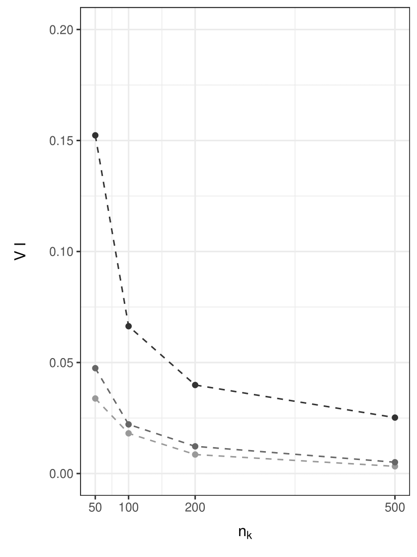
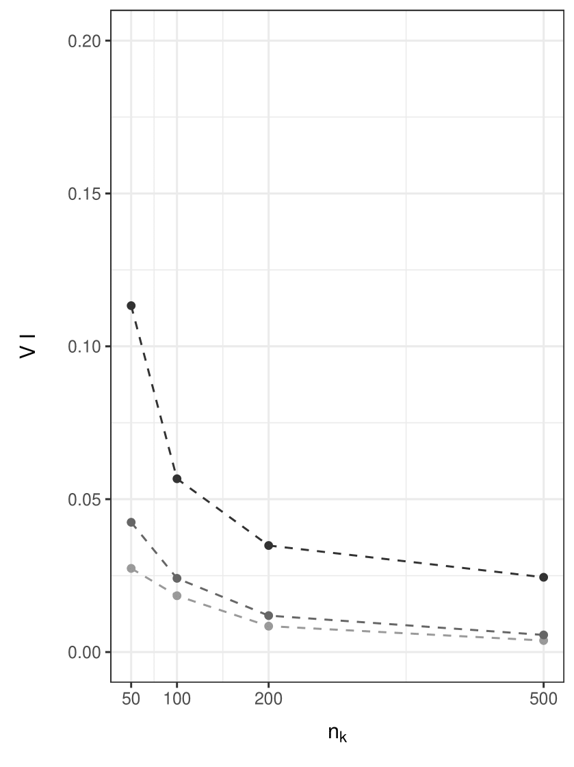
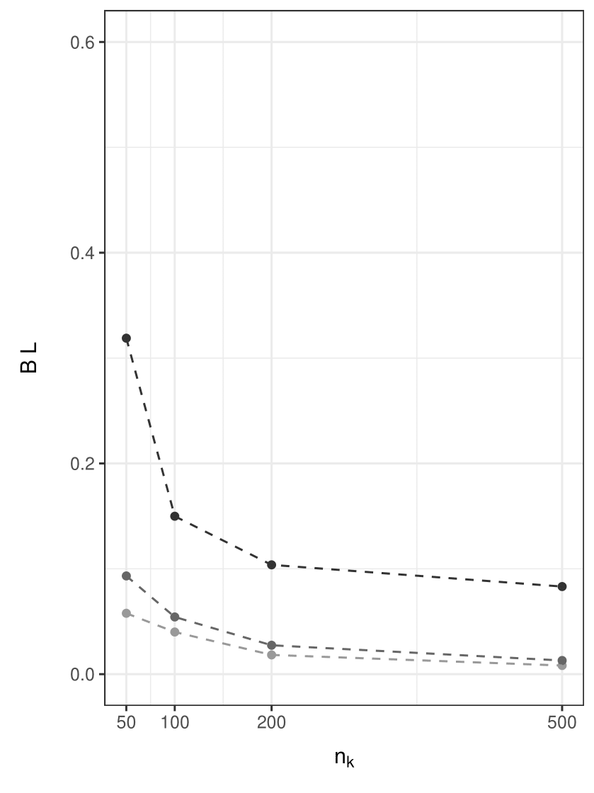
We first evaluate the performance of our method with regard to cluster allocation. To this end, we compare the true partition with the estimated partition by means of the Binder Loss (BL) [4] and the Variation of Information (VI) [27]. The two metrics, normalized in are respectively defined as
with and representing the entropy associated to clustering , and the mutual information between the two clusterings , where and ; see also Meilă [27]. Intuitively, lower values of the two indexes correspond to better performances in the clustering allocation. We compute BL and VI under each simulated dataset and scenario. Results are summarized in the plots of Figure 1. Each sequence of points joined by a dotted line represents the average values (w.r.t. the simulations) of an index computed for increasing sample sizes and one value of (with increasing values of from dark to light grey). It appears that the performance of the method improves as grows under each scenario both in terms of BL and VI. Moreover, higher values of make cluster identification easier even for moderate sample sizes, e.g. . In addition, the clustering performance is better under Different DAGs scenario which corresponds to settings with DAGs generated independently and therefore also “structurally” different.
| Equal DAGs | Different DAGs |
|---|---|
 |
 |
 |
 |
5.3 Structural learning
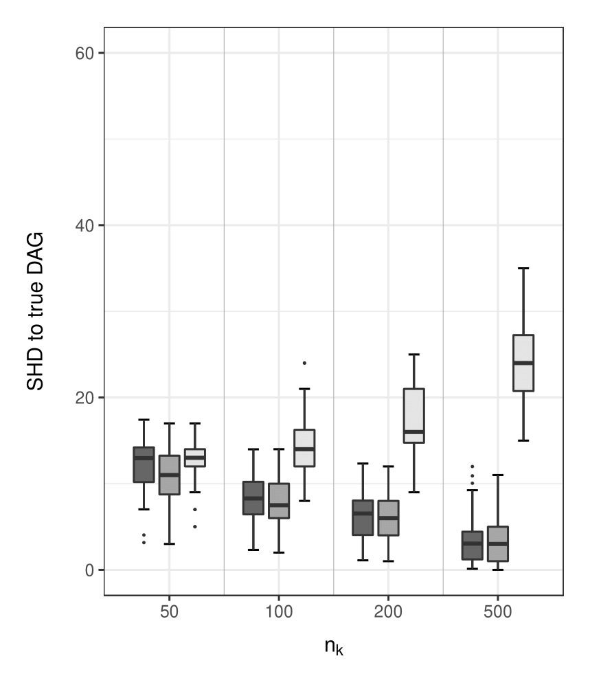
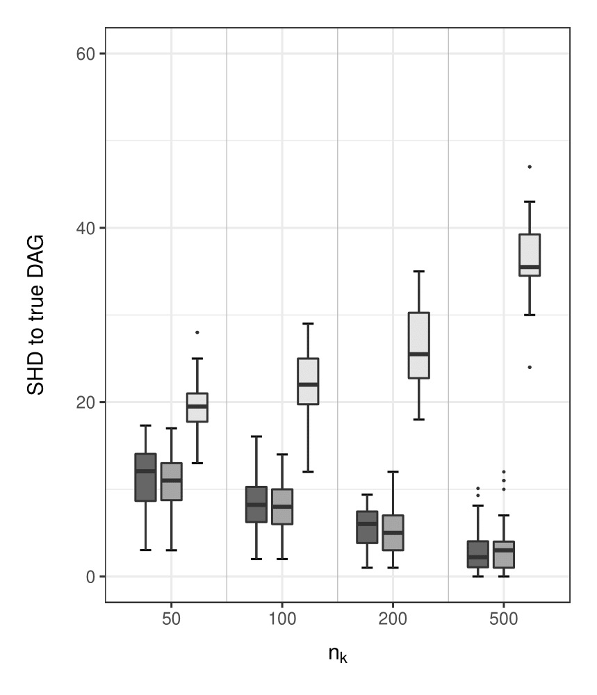
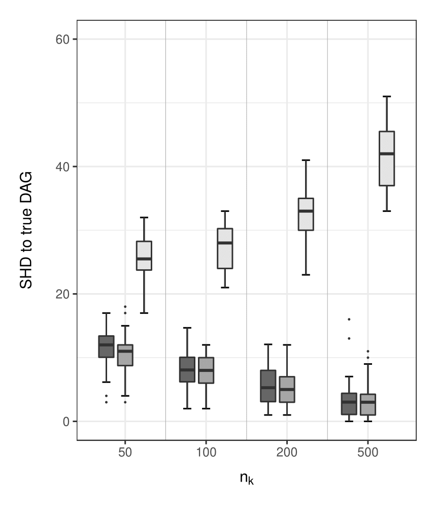
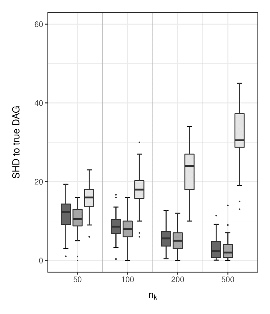
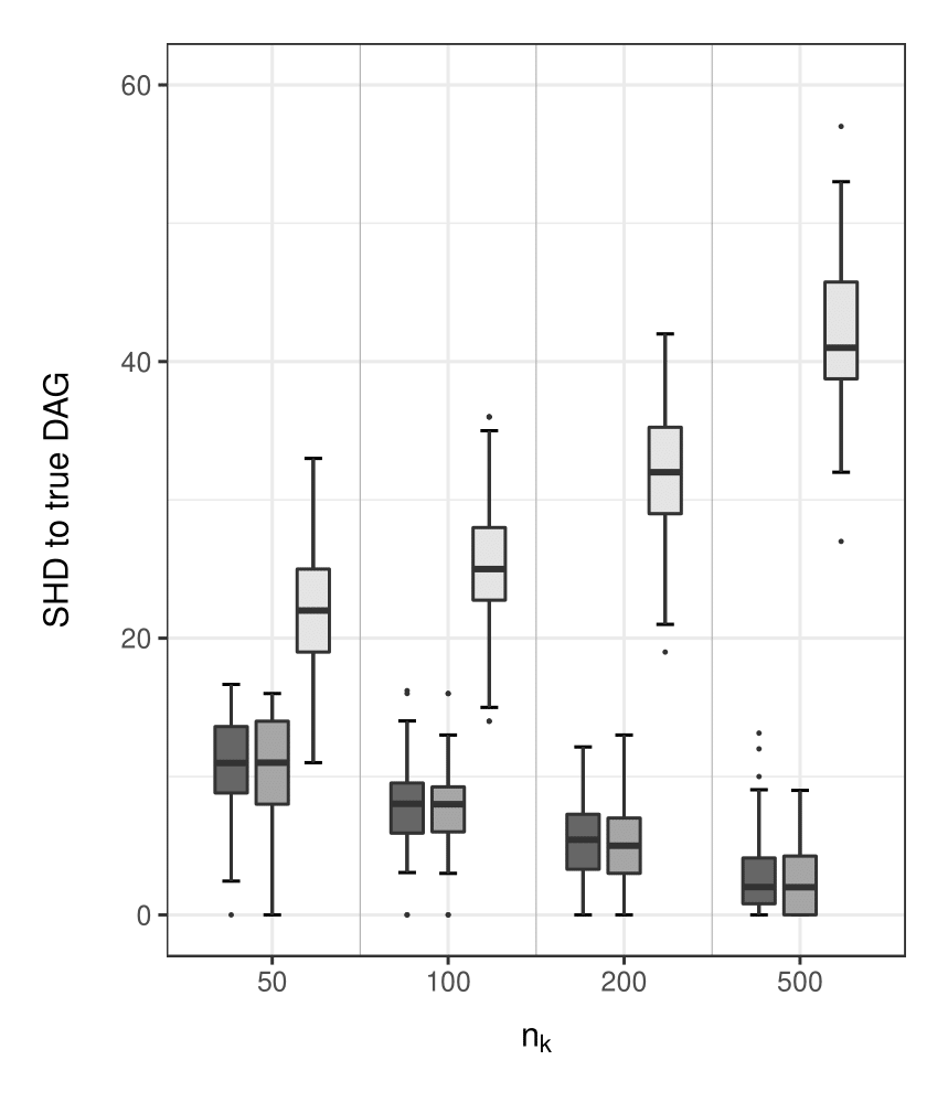
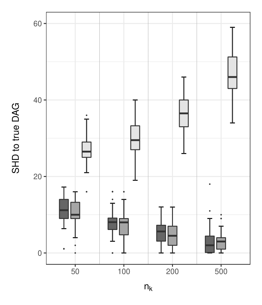
We now evaluate the performance of our method in learning the graph structures. To this end, under each simulation, we measure the Structural Hamming Distance (SHD) between each (individual) estimated DAG , and the corresponding true DAG. SHD corresponds to the number of edge insertions, deletions or flips needed to transform the estimated DAG into the true one; accordingly, lower values of SHD correspond to better performances.
For comparison purposes, we also include two alternative, yet opposed, learning strategies which are not based on DP mixture models. The first one corresponds to an oracle setting wherein the true two-group clustering is known beforehand. We call this benchmark Two-group oracle. The second instead wrongly assumes that all observations are conditionally iid from the same one-component model, and we name it One-group naive. Both benchmarks try to evaluate differential performance in structural learning: the former assesses the gain afforded by removing imperfect knowledge on clustering; the latter instead captures decay due to naively neglecting heterogeneity. In both benchmark strategies, while not running a DP mixture model, we use the same specifications for the prior on DAG- and parameter space.
Results, for each of the two scenarios Equal DAGs and Different DAGs, are summarized in the plots of Figure 2. Each box-plot represents the distribution of SHD, averaged with respect to individuals belonging to the same true cluster, with increasing group sample size , and increasing values of (from top to bottom row). It appears that One-group naive performs worse w.r.t. the other two methods under both scenarios. In particular its performance worsens as increases and for larger values of , because under both circumstances the two clusters become better separated. Reassuringly, Two-group oracle performs only slightly better than our DP mixture method even in the setting , where cluster identification is more difficult, with results nearly indistinguishable for . In addition, both methods improve their performance as grows.
| Equal DAGs | ||
 |
 |
 |
| Different DAGs | ||
 |
 |
 |
5.4 Causal effect estimation
We finally consider causal effect estimation. Under each scenario, we compare the collection of subject-specific BMA causal effect estimates , , , in Equation (19) with the corresponding true causal effects by means of the absolute-value distance
The distribution of across subjects and simulated datasets is summarized through the average distance whose percentage values, computed under each scenario, are reported in Tables 1 and 2; the two tables refer to scenarios Equal DAGs and Different DAGs respectively. For comparisons, we also compute the same collection of causal effect estimates under Two-group oracle. It appears that, while both methods improve their performances as and grows, DP mixtures performs only slightly worse than Two-group oracle. In addition, such differences are more evident under scenarios with moderate sample size and smaller values of , e.g. , where indeed cluster allocation was also more difficult.
| 50 | 100 | 200 | 500 | ||
|---|---|---|---|---|---|
| DP mixture | 3.18 | 2.75 | 2.15 | 1.60 | |
| Two-group oracle | 2.72 | 2.56 | 2.00 | 1.47 | |
| DP mixture | 3.41 | 2.90 | 2.25 | 1.72 | |
| Two-group oracle | 2.80 | 2.70 | 2.05 | 1.63 | |
| DP mixture | 3.65 | 2.91 | 2.25 | 1.63 | |
| Two-group oracle | 2.90 | 2.56 | 2.04 | 1.41 |
| 50 | 100 | 200 | 500 | ||
|---|---|---|---|---|---|
| DP mixture | 3.44 | 2.91 | 2.66 | 1.70 | |
| Two-group oracle | 3.10 | 2.63 | 2.60 | 1.67 | |
| DP mixture | 3.83 | 2.97 | 2.64 | 1.80 | |
| Two-group oracle | 3.18 | 2.66 | 2.60 | 1.64 | |
| DP mixture | 4.19 | 3.06 | 2.74 | 1.90 | |
| Two-group oracle | 3.00 | 2.64 | 2.59 | 1.79 |
6 Analysis of AML data
In this section we apply our methodology to the protein dataset of patients affected by Acute Myeloid Leukemia (AML) described in the Introduction. This dataset contains the level of proteins and phosphoproteins involved in apoptosis and cell cycle regulation according to the KEGG database [21] for 256 newly diagnosed AML patients and is provided as a supplement to Kornblau et al. [22]. Classification of AML patients is commonly based on the French-American-British (FAB) system and relies on morphologic features, along with flow cytometric analysis of surface marker expression, cytogenetics, and assessment of recurrent molecular abnormalities. In particular, 11 of the FAB subtypes are present in the dataset, besides one group of patients with unknown subtype; see also Table 3.
| subtype | M0 | M1 | M2 | M4 | M4EOS | M5 | M5A | M5b | M6 | M7 | RAEBT | Unknown |
|---|---|---|---|---|---|---|---|---|---|---|---|---|
| size | 17 | 34 | 68 | 59 | 9 | 6 | 13 | 9 | 7 | 5 | 5 | 24 |
The same dataset was analysed by Peterson et al. [35] and Castelletti et al. [9] from a multiple graphical model-perspective. These Authors included in their analysis four AML subtypes for which a reasonable sample size is available: M0 (17 subjects), M1 (34 subjects), M2 (68 subjects), and M4 (59 subjects). Specifically, assuming the four groups were given, both papers developed a Bayesian analysis which allows potentially common features in graphical structures - undirected in the first paper and directed in the second one - to be shared among groups. In the end, both methods revealed strong similarities between groups in terms of the estimated protein-network structures, but at the same time they were able to identify a few protein interactions specific to a given subtype. In this paper we take a different approach, and apply our mixture model to the full dataset (including all the subjects) without grouping the patients a priori, but rather letting the model cluster the observations as it learns the graphical structuret of protein-interactions. Eventually, we also evaluate the effect of interventions on proteins in the network at a subject-specific level.
Among the proteins included in the study, AKT belongs to the phosphoinositide 3-kinase (PI3K)-Akt-mammalian target of rapamycin (mTOR) pathway (PI3K-Akt-mTOR pathway) which is one of the intracellular pathways aberrantly up-regulated in AML [30]. Activation of this pathway (e.g. induced by AKT regulation) has been established to play an important role in leukemogenesis. In addition, targeting the PI3K-Akt-mTOR pathway with specific inhibitors may produce different effects on AML patients, reflecting biological heterogeneity in the intracellular signaling status [12]. Because of the role played in AML progression and response to therapy, we therefore consider the AKT protein and phosphoproteins (AKT, AKT.p308, AKT.p473 in the following) as responses of interest for our causal-effect analysis.
We implement the proposed model by running our MCMC scheme for iterations, which includes a burn-in period of runs. We fix hyper-parameters , in the Gamma prior on the precision parameter , which is consistent with a moderate expected number of clusters . In addition, we set , , , in the Normal-DAG-Wishart prior as in the simulation settings of Section 5.1. With regard to the Beta prior on the probability of edge inclusion we instead fix , , which reflects a moderate degree of sparsity in the network. To assess the convergence of our algorithm we also run independent MCMC chains with results suggesting a highly satisfactory agreement in terms of clustering, graph structure learning and causal effect estimation; see also the Supplementary material for further details.
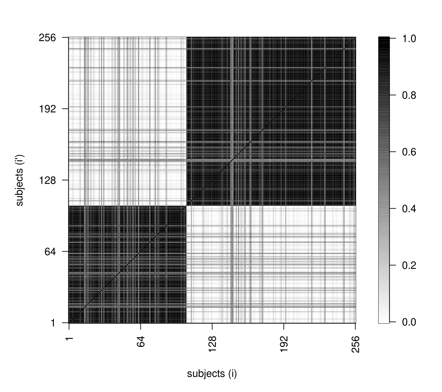
Starting from the MCMC output we first produce the similarity matrix based on the posterior probabilities (17) computed for each pair of subjects . In particular, fixing a threshold for clustering inclusion equal to , we obtain a partition with two groups of size . For ease of interpretation we numbered subjects in cluster 1 from 1 to 105, followed by those in cluster 2 from 106 to 256. Results are summarized in the heat map of Figure 3 where the axes report the ordered subjects. We note that in both estimated clusters there exist a few subjects appearing to be borderline in the sense that they barely qualify for membership to the assigned group (their inclusion probabilities in groups 1 and 2 are approximatively equal).
 |
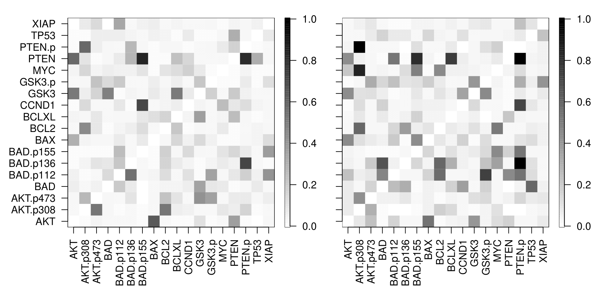
We now focus on graph structure learning. Specifically, we construct for each subject a matrix collecting the posterior inclusion probabilities of each (directed) edge , . Results for two randomly chosen subjects, whose membership is estimated to be cluster 1 and cluster 2 respectively, are reported in Figure 4. The two heat maps reveal an appreciable degree of sparsity in each of the two underlying DAG structures, together with some noticeable differences in the network links.
 |
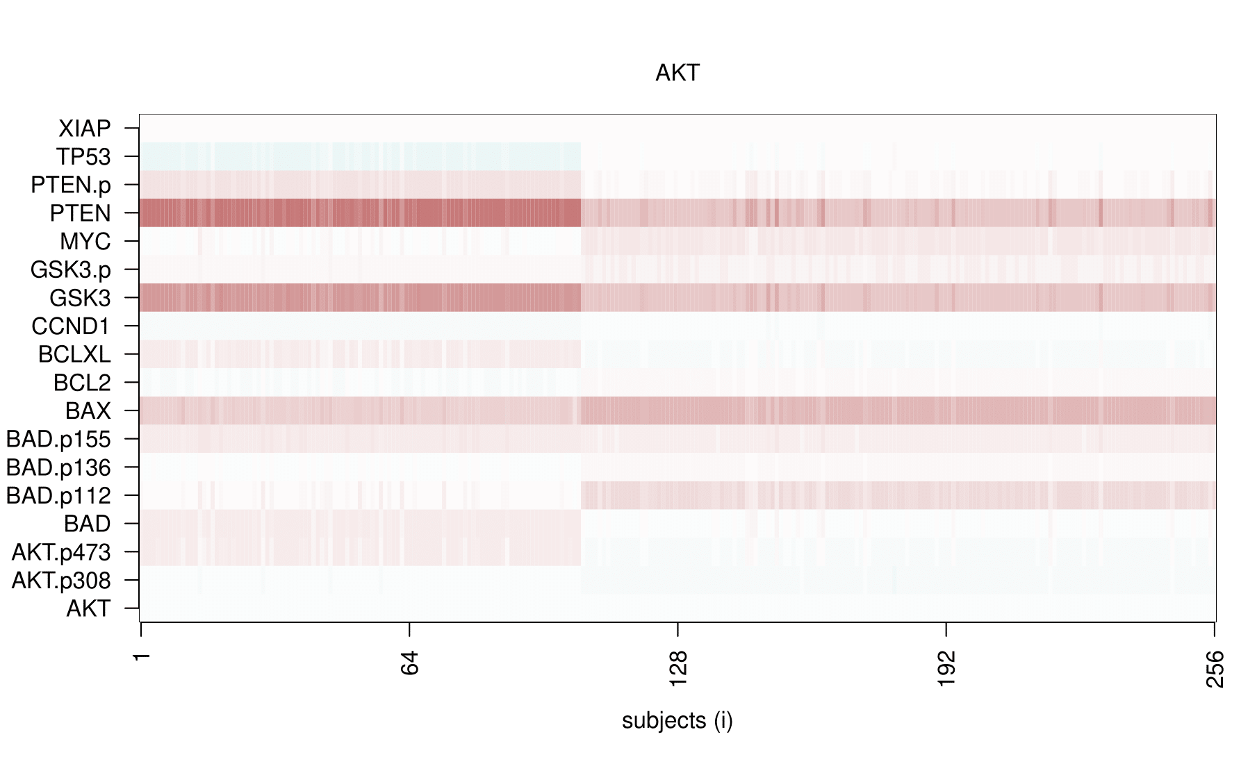
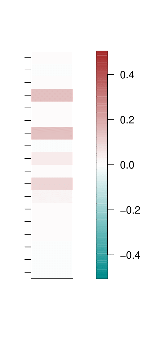
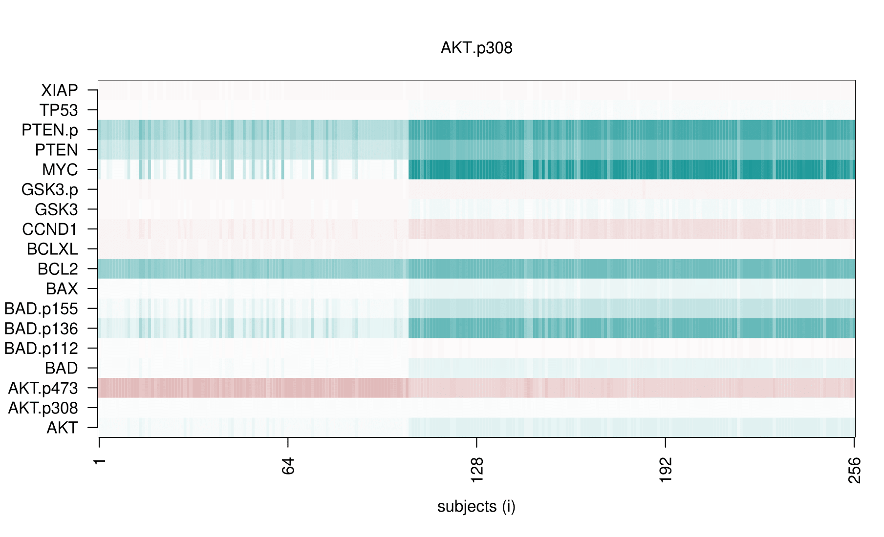
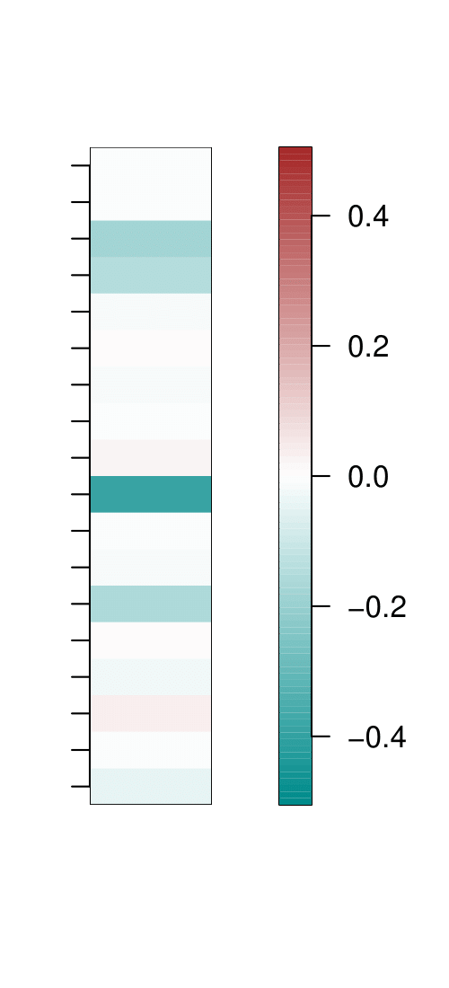
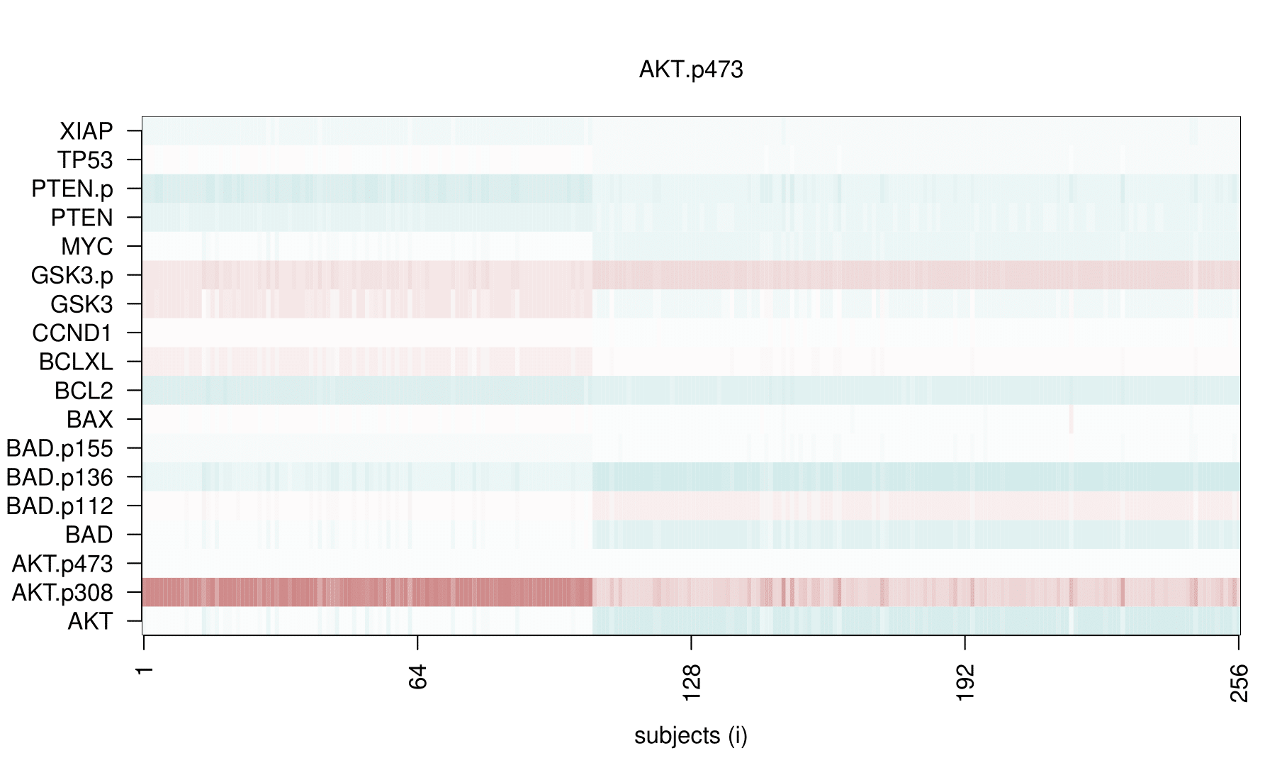
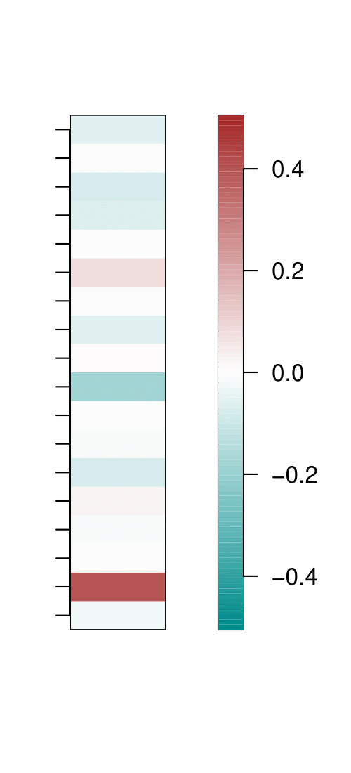
Using Equation (19), we can provide a subject-specific BMA estimate of the causal effect on each of the responses AKT, AKT.p308, AKT.p473 following an intervention on any other protein in the network leading to the collection , for each subject . Results are summarized in the heat maps of Figure 5 where each plot refers to one of the three response variables. The pattern already observed in Figure 3 is also apparent. Subjects assigned to the same cluster reveal broadly similar causal effect estimates, with some notable exceptions in both groups for a few individuals.
More interestingly, the effect of an intervention varies across the two groups, showing that the cluster structure produced by our analysis has a causal counterpart. Take for instance the effect of protein PTEN onto AKT: this is more strongly positive in group 1 than in group 2. Conversely, if the response is AKT.p308 the effect in both groups is negative, and more pronounced in group 2. This finding is of potential interest as protein PTEN has been identified as a tumor suppressor because it is capable of breaking the PI3K-Akt-mTOR pathway, and therefore represents a common target for inactivation in cancers [5, 17]. From a personalized therapy perspective, one can then argue that AKT regulation can be induced through interventions which however should be selected at subject-specific level, because they can result in heterogeneous causal effects - and corresponding levels of efficacy - across different subjects.
In addition, to appreciate the role played by population heterogeneity in causal effect estimation, we compare our results with those based on the alternative One-group naive strategy (Section 5.3). Results are included in the right-side maps of Figure 5.
Clearly, in this setting, causal effects following any intervention are equal across subjects. This output reveals substantial differences relative to our previous analysis suggesting that methods which neglect population heterogeneity can produce misleading estimates of causal effects. In particular, the one-group assumption has in some cases a “dilution” effect on coefficients’ estimates. This means that each causal effect obtained from One-group naive is akin to an average of cluster-specific causal estimates which are substantially different among groups. This happens for instance with regard to response AKT for causal effects associated with protein PTEN. Here, the causal effect obtained from One-group naive corresponds to a value in between the collection of causal effects resulting from DP mixture. As a consequence the ensuing causal effect coefficient provides an inadequate quantification of the underlying effect because it under- and over- estimates causal effects for individuals in clusters 1 and 2 respectively.
|
|
|
Common practice would suggest to first cluster patients into groups according to selected covariates, whenever available, and then infer DAGs and causal effects for each group separately. In this connection, the leukemia subtypes (Table 3) may be used for this purpose. A comparison with this alternative approach is provided in the Supplementary material, where it is shown that patients belonging to some subtypes, in particular M0, M1, M2, are not primarily assigned to either estimated cluster. As a consequence, for subjects belonging to these subtypes there are substantial differences in the resulting causal effect estimates. This finding suggests that methods which only rely on a pre-determined group classification may produce inaccurate and possibly misleading estimates of causal effects.
7 Discussion
In this paper we present a Bayesian framework to evaluate heterogeneous causal effects based on Directed Acyclic Graphs (DAGs). We model heterogeneity through an infinite mixture model which accounts both for structure and parameter uncertainty. The output of our methodology is a collection of subject-specific causal effects, each being a Bayesian model average of causal effects across DAGs. Because of the discreteness of the process governing the generation of the individual parameters, a posterior distribution on the clustering structure of the units is also available.
Our analysis is based on a Dirichlet Process (DP) mixture of Gaussian DAG models. While more general Bayesian nonparametric models might be adopted, e.g. Müller & Mitra [28], and Barrios et al. [2], we believe that the main content of our contribution, namely causal inference under heterogeneity based on DAGs, is best captured by the current DP mixture model because of its popularity, interpretability and simplicity of implementation.
Protein and gene expression levels are known to be affected by genetic, environmental, demographic, and other factors. This means that, in addition to the measured variables, there will typically be sources of heterogeneity which are hidden or latent, and failing to incorporate these sources may have detrimental effects on the study [25]. Currently we do not consider latent variables in our model. In principle they could be made part of our setup, along the lines of Frot et al. [15] for structure learning, and of Shpitser & Tchetgen Tchetgen [43] for the identification of causal effects, although this would add a significant layer of complexity to the whole procedure.
The type of interventions we have considered may be called perfect, meaning that they eliminate dependencies between targeted variables and their direct causes; the identifiability of causal DAGs under perfect interventions was characterized by Hauser & Bühlmann [20]. More recently the broader notion of general intervention has been introduced, which may modify the dependencies between targeted variables and their causes without eliminating them; see Yang et al. [48].
Acknowledgments This research was partially supported by UCSC (D1 and 2019-D.3.2 research grants). We thank Raffaele Argiento for useful discussions on the slice sampler.
SUPPLEMENTARY MATERIAL
The file supplementary_material.pdf provides supplemental information to our paper, which is organized into three sections. Section 1 contains a detailed description of the elicitation procedure leading to compatible priors for DAG-model parameters based on Normal-DAG-Wishart distributions. Section 2 describes our MCMC scheme for posterior inference on DAG structures, cluster allocation parameters and causal effects. Finally, Section 3 provides convergence diagnostics relative to the application on AML data and additional results.
References
- Athey & Imbens [2016] Athey, S. & Imbens, G. (2016). Recursive partitioning for heterogeneous causal effects. Proceedings of the National Academy of Sciences 113 7353–7360.
- Barrios et al. [2013] Barrios, E., Lijoi, A., Nieto-Barajas, L. E. & Prünster, I. (2013). Modeling with normalized random measure mixture models. Statistical Science 28 313–334.
- Bühlmann [2020] Bühlmann, P. (2020). Invariance, causality and robustness. Statistical Science 35 404–426.
- Binder [1978] Binder, D. A. (1978). Bayesian cluster analysis. Biometrika 65 31–38.
- Cantley & Neel [1999] Cantley, L. & Neel, B. (1999). New insights into tumor suppression: PTEN suppresses tumor formation by restraining the phosphoinositide 3-kinase/AKT pathway. Proceedings of the National Academy of Sciences 8 4240–4245.
- Cao et al. [2019] Cao, X., Khare, K. & Ghosh, M. (2019). Posterior graph selection and estimation consistency for high-dimensional Bayesian DAG models. The Annals of Statistics 47 319–348.
- Castelletti & Consonni [2021a] Castelletti, F. & Consonni, G. (2021a). Bayesian causal inference in probit graphical models. Bayesian Analysis 1 – 25.
- Castelletti & Consonni [2021b] Castelletti, F. & Consonni, G. (2021b). Bayesian inference of causal effects from observational data in Gaussian graphical models. Biometrics 77 136–149.
- Castelletti et al. [2020] Castelletti, F., La Rocca, L., Peluso, S., Stingo, F. C. & Consonni, G. (2020). Bayesian learning of multiple directed networks from observational data. Statistics in Medicine 39 4745–4766.
- Cremaschi et al. [2019] Cremaschi, A., Argiento, R., Shoemaker, K., Peterson, C. & Vannucci, M. (2019). Hierarchical normalized completely random measures for robust graphical modeling. Bayesian Analysis 14 1271–1301.
- Escobar & West [1995] Escobar, M. D. & West, M. (1995). Bayesian density estimation and inference using mixtures. Journal of the American Statistical Association 90 577–588.
- Estruch et al. [2021] Estruch, M., Reckzeh, K., Vittori, C., Centio, A., Ali, M., Engelhard, S., Zhao, L., Won, K., Liu, P., Porse, B. & Theilgaard-Mönch, K. (2021). Targeted inhibition of cooperative mutation- and therapy-induced AKT activation in AML effectively enhances response to chemotherapy. Leukemia 2030–2042.
- Finegold & Drton [2011] Finegold, M. & Drton, M. (2011). Robust graphical modeling of gene networks using classical and alternative -distributions. The Annals of Applied Statistics 5 1057–1080.
- Finegold & Drton [2014] Finegold, M. & Drton, M. (2014). Robust Bayesian graphical modeling using Dirichlet -distributions. Bayesian Analysis 9 521–550.
- Frot et al. [2019] Frot, B., Jostins, L. & McVean, G. (2019). Graphical model selection for Gaussian conditional random fields in the presence of latent variables. Journal of the American Statistical Association 114 723–734.
- Geiger & Heckerman [2002] Geiger, D. & Heckerman, D. (2002). Parameter priors for directed acyclic graphical models and the characterization of several probability distributions. The Annals of Statistics 30 1412–1440.
- Georgescu [2012] Georgescu, M. (2012). PTEN tumor suppressor network in PI3K-Akt pathway control. Genes Cancer 12 1170–1177.
- Godsill [2012] Godsill, S. J. (2012). On the relationship between Markov chain Monte Carlo methods for model uncertainty. Journal of Computational and Graphical Statistics 10 230–248.
- Hahn et al. [2020] Hahn, P. R., Murray, J. S. & Carvalho, C. M. (2020). Bayesian regression tree models for causal inference: regularization, confounding, and heterogeneous effects (with discussion). Bayesian Analysis 15 965–1056.
- Hauser & Bühlmann [2012] Hauser, A. & Bühlmann, P. (2012). Characterization and greedy learning of interventional Markov equivalence classes of directed acyclic graphs. Journal of Machine Learning Research 13 2409–2464.
- Kanehisa et al. [2012] Kanehisa, M., Goto, S., Sato, Y., Furumichi, M. & Tanabe, M. (2012). KEGG for integration and interpretation of large-scale molecular data sets. Nucleic Acids Research D109–D114.
- Kornblau et al. [2009] Kornblau, S., Tibes, R., Qiu, Y., Chen, W., Kantarjian, H., Andreeff, M., Coombes, K. & Mills, G. (2009). Functional proteomic profiling of AML predicts response and survival. Blood 1 154–164.
- Lauritzen [1996] Lauritzen, S. L. (1996). Graphical models. Oxford University Press.
- Lee et al. [2020] Lee, K., Bargagli-Stoffi, F. J. & Dominici, F. (2020). Causal rule ensemble: interpretable inference of heterogeneous treatment effects. ArXiv preprint, 2009.09036.
- Leek & Storey [2007] Leek, J. T. & Storey, J. (2007). Capturing heterogeneity in gene expression studies by surrogate variable analysis. PLoS Genetics 3 1724–1735.
- Maathuis & Nandy [2016] Maathuis, M. & Nandy, P. (2016). A review of some recent advances in causal inference. In P. Bühlmann, P. Drineas, M. Kane & M. van der Laan, eds., Handbook of Big Data. Chapman and Hall/CRC, 387–408.
- Meilă [2007] Meilă, M. (2007). Comparing clusterings - an information based distance. Journal of Multivariate Analysis 98 873–895.
- Müller & Mitra [2013] Müller, P. & Mitra, R. (2013). Bayesian nonparametric inference – why and how. Bayesian Analysis 8 269–302.
- Murugiah & Sweeting [2012] Murugiah, S. & Sweeting, T. (2012). Selecting the precision parameter prior in Dirichlet process mixture models. Journal of Statistical Planning and Inference 142 1947–1959.
- Nepstad et al. [2020] Nepstad, I., Hatfield, K., Grønningsæter, I. & H., R. (2020). The PI3K-Akt-mTOR signaling pathway in human acute myeloid leukemia (AML) cells. International Journal of Molecular Sciences 21.
- Ni et al. [2017] Ni, Y., Stingo, F. C. & Baladandayuthapani, V. (2017). Sparse multi-dimensional graphical models: a unified Bayesian framework. Journal of the American Statistical Association 112 779–793.
- Oganisian et al. [2021] Oganisian, A., Mitra, N. & Roy, J. A. (2021). A Bayesian nonparametric model for zero-inflated outcomes: Prediction, clustering, and causal estimation. Biometrics 77 125–135.
- Pearl [2000] Pearl, J. (2000). Causality: models, reasoning, and inference. Cambridge University Press, Cambridge.
- Peters & Bühlmann [2014] Peters, J. & Bühlmann, P. (2014). Identifiability of Gaussian structural equation models with equal error variances. Biometrika 101 219–228.
- Peterson et al. [2015] Peterson, C., Stingo, F. C. & Vannucci, M. (2015). Bayesian inference of multiple Gaussian graphical models. Journal of the American Statistical Association 110 159–174.
- Rodríguez et al. [2011] Rodríguez, A., Lenkoski, A. & Dobra, A. (2011). Sparse covariance estimation in heterogeneous samples. Electronic Journal of Statistics 5 981–1014.
- Roy et al. [2016] Roy, J., Lum, K. J. & Daniels, M. J. (2016). A Bayesian nonparametric approach to marginal structural models for point treatments and a continuous or survival outcome. Biostatistics 18 32–47.
- Rubin [1974] Rubin, D. B. (1974). Estimating causal effects of treatments in randomized and nonrandomized studies. Journal of Educational Psychology 66 688–701.
- Rubin [2005] Rubin, D. B. (2005). Causal inference using potential outcomes. Journal of the American Statistical Association 100 322–331.
- Scott & Berger [2010] Scott, J. G. & Berger, J. O. (2010). Bayes and empirical-Bayes multiplicity adjustment in the variable-selection problem. The Annals of Statistics 38 2587–2619.
- Shen et al. [2009] Shen, R., Olshen, A. B. & Ladanyi, M. (2009). Integrative clustering of multiple genomic data types using a joint latent variable model with application to breast and lung cancer subtype analysis. Bioinformatics 25 2906–2912.
- Shpitser & Sherman [2018] Shpitser, I. & Sherman, E. (2018). Identification of personalized effects associated with causal pathways. In Proceedings of the 34th Annual Conference on Uncertainty in Artificial Intelligence, UAI-18.
- Shpitser & Tchetgen Tchetgen [2016] Shpitser, I. & Tchetgen Tchetgen, E. (2016). Causal inference with a graphical hierarchy of interventions. The Annals of Statistics 44 2433–2466.
- Wager & Athey [2018] Wager, S. & Athey, S. (2018). Estimation and inference of heterogeneous treatment effects using random forests. Journal of the American Statistical Association 113 1228–1242.
- Walker [2007] Walker, S. G. (2007). Sampling the Dirichlet mixture model with slices. Communications in Statistics - Simulation and Computation 36 45–54.
- Wilkerson & Hayes [2010] Wilkerson, M. D. & Hayes, D. N. (2010). ConsensusClusterPlus: a class discovery tool with confidence assessments and item tracking. Bioinformatics 26 1572–1573.
- Witte et al. [2020] Witte, J., Henckel, L., Maathuis, M. H. & Didelez, V. (2020). On efficient adjustment in causal graphs. Journal of Machine Learning Research 21 1–45.
- Yang et al. [2018] Yang, K., Katcoff, A. & Uhler, C. (2018). Characterizing and learning equivalence classes of causal DAGs under interventions. In J. Dy & A. Krause, eds., Proceedings of the 35th International Conference on Machine Learning, vol. 80 of Proceedings of Machine Learning Research. PMLR, 5541–5550.
- Zhang et al. [2017] Zhang, W., Le, T. D., Liu, L., Zhou, Z.-H. & Li, J. (2017). Mining heterogeneous causal effects for personalized cancer treatment. Bioinformatics 33 2372–2378.
