Statistical Inference for Cox Proportional Hazards Models with a Diverging Number of Covariates

Abstract

For statistical inference on regression models with a diverging number of covariates, the existing literature typically makes sparsity assumptions on the inverse of the Fisher information matrix. Such assumptions, however, are often violated under Cox proportion hazards models, leading to biased estimates with under-coverage confidence intervals. We propose a modified debiased lasso approach, which solves a series of quadratic programming problems to approximate the inverse information matrix without posing sparse matrix assumptions. We establish asymptotic results for the estimated regression coefficients when the dimension of covariates diverges with the sample size. As demonstrated by extensive simulations, our proposed method provides consistent estimates and confidence intervals with nominal coverage probabilities. The utility of the method is further demonstrated by assessing the effects of genetic markers on patients’ overall survival with the Boston Lung Cancer Survival Cohort, a large-scale epidemiology study investigating mechanisms underlying the lung cancer.

Keywords: Confidence interval, Cox proportional hazards model, Debiased lasso, Diverging dimension, Sparsity, Statistical inference.

1 Introduction

The Cox proportional hazards model (Cox,, 1972), a semiparametric model with an unspecified baseline hazard function, has been widely used for the analysis of censored time-to-event data. With a fixed dimension of covariates, Cox, (1972) proposed the maximum partial likelihood estimation (MPLE) to infer the regression coefficients, and Andersen and Gill, (1982) proved the asymptotic distributional results for MPLE using the Martingale theory.

Technological advances nowadays have made it possible to collect a large amount of information in biomedical studies. For example, the Boston Lung Cancer Survival Cohort (BLCSC), the motivating study for this work, has acquired abundant clinical, genetic, epigenetic and genomic data, which enable comprehensive investigations of molecular mechanisms underlying the lung cancer survival (McKay et al.,, 2017). High-dimensionality of the collected covariates has confronted the traditional parameter estimation and uncertainty quantification based on Cox models. In high-dimensional settings, where the number of covariates $p$ increases with the sample size $n$ or even greater than $n$, the conventional maximum partial likelihood estimation is usually ill-conditioned. Penalized estimators have emerged as a powerful tool for simultaneous variable selection and estimation (Tibshirani,, 1997; Fan and Li,, 2002; Gui and Li,, 2005; Antoniadis et al.,, 2010). Recently, Huang et al., (2013) and Kong and Nan, (2014) derived the non-asymptotic oracle inequalities of the lasso estimator in the Cox model. However, none of these works dealt with statistical inference for Cox models with high-dimensional covariates.

Existing literature on inference for high-dimensional models mainly concerns linear regression. Zhang and Zhang, (2014), van de Geer et al., (2014) and Javanmard and Montanari, (2014) developed inference procedures for linear models, based on debiasing the lasso estimator via low-dimensional projection or inverting the Karush–Kuhn–Tucker condition. van de Geer et al., (2014) extended the debiased lasso idea to generalized linear models, using the nodewise lasso regression. Ning and Liu, (2017) focused on hypothesis testing and devised decorrelated score, Wald and likelihood ratio tests for inference on a low-dimensional parameter in generalized linear models based on projection theory.

There has been limited progress in inference for the Cox model with high-dimensional covariates. Fang et al., (2017) developed decorrelated tests for hypothesis testing of low-dimensional components under high-dimensional Cox models, using ideas similar to Ning and Liu, (2017). Kong et al., (2018) extended the debiased lasso approach in van de Geer et al., (2014) to potentially misspecified Cox models, and used the nodewise lasso regression to estimate the inverse information matrix. Yu et al., (2018) proposed a debiased lasso approach, by estimating the inverse information matrix with a CLIME estimator adapted from (Cai et al.,, 2011). Most of these works restricted the number of non-zero elements of each row in the inverse information matrix to be small, i.e. $\ell_{0}$ sparsity. However, as found in Xia et al., (2020), the sparse inverse information matrix assumption has no practical interpretation beyond linear regression models, often fails to hold in the Cox model, and these methods cannot perform satisfactorily in high-dimensional Cox model settings. For example, as evidenced by our extensive simulations, these methods cannot correct biases of lasso estimators or construct confidence intervals with desired coverage probabilities, even when the number of regression coefficients is moderate relative to the sample size.

Our work is pertaining to the “large $n$, diverging $p$” framework where $p<n$ and $p$ is allowed to increase with $n$ to infinity, which reflects the setting of the motivating BLCSC with $n=561$ and $p=231$. Under this framework, we draw inference based on Cox models without imposing sparsity to the inverse information matrix. Specifically, we propose a debiased lasso approach via solving a series of quadratic programming problems to estimate the inverse information matrix. We use quadratic programming as a means of balancing the bias-variance trade-off and avoiding the unrealistic $\ell_{0}$ sparsity assumption for the large inverse information matrix in the Cox model. Our work adds to the literature in the following aspects. First, unlike Javanmard and Montanari, (2014), our work entails careful treatment of the sum of non independently nor identically distributed terms in the empirical loss function, and we consider random designs instead of deterministic designs. Second, we find that the tuning parameter selection for the inverse information matrix estimation is crucial for bias correction. For example, a related work (Yu et al.,, 2018) proposed to select tuning parameters by minimizing the cross-validated difference between the product of the information matrix with its estimated inverse and the identity matrix, but was found to perform poorly. In contrast, we propose a cross-validation procedure to tune parameters by hard thresholding debiased estimates when solving the quadratic programming problems, which yields satisfactory numerical performance.

The article is organized as follows. Section 2 introduces the proposed debiased lasso approach, where the inverse information matrix is estimated via quadratic programming with a novel cross-validation procedure for selecting the tuning parameter. Section 3 lays the theoretical foundation for reliable inference on linear combinations of the Cox regression parameters using debiased lasso estimators. We examine the finite sample performance of our proposed method with simulation studies in Section 4, apply it to analyze the BLCSC data in Section 5, and conclude the paper with a few remarks in Section 6. We state several useful technical lemmas and provide proofs of the main theorems in the Appendix, and defer proofs of all the lemmas to the online supplementary materials.

2 Method

2.1 Background and set-up

We introduce notation that will be used throughout this article. For a vector $x=(x_{1},\ldots,x_{r})^{T}\in\mathbb{R}^{r}$, $x^{\otimes 0}=1$, $x^{\otimes 1}=x$ and $x^{\otimes 2}=xx^{T}$. The $\ell_{q}$-norm for $x$ is $\|x\|_{q}=(\sum_{j=1}^{r}|x_{j}|^{q})^{1/q}$, $q\geq 1$, and the $\ell_{0}$-norm is $\|x\|_{0}=\sum_{j=1}^{r}I(x_{j}\neq 0)$. For a matrix $A=(a_{ij})\in\mathbb{R}^{m\times r}$, the induced matrix norm is defined as $\|A\|_{q_{1},q_{2}}=\sup_{x\in\mathbb{R}^{r},x\neq 0}\|Ax\|_{q_{2}}/\|x\|_{q_{1}}$, $q_{1},q_{2}\geq 1$. In particular, $\|A\|_{1,1}=\max_{1\leq j\leq r}\sum_{i=1}^{m}|a_{ij}|$, $\|A\|_{2,2}=\sigma_{\mathrm{max}}(A)$, the largest singular value of $A$, and $\|A\|_{\infty,\infty}=\max_{1\leq i\leq m}\sum_{j=1}^{r}|a_{ij}|$. The element-wise max norm is denoted as $\|A\|_{\infty}=\max_{i,j}|a_{ij}|$. For two positive sequences $\{d_{n}\}$ and $\{g_{n}\}$, we define $d_{n}\asymp g_{n}$ if there are two bounded positive constants $C$ and $C^{\prime}$ such that $C\leq d_{n}/g_{n}\leq C^{\prime}$.

A Cox model stipulates that the hazard function for the underlying failure time $T$, conditional on a $p$-dimensional vector of covariates $X=(X^{(1)},\ldots,X^{(p)})\in\mathbb{R}^{p}$, is $h(t|X)=h_{0}(t)\exp\{X^{T}\beta^{0}\}$, where $h_{0}(t)$ is an unknown baseline hazard function and $\beta^{0}=(\beta^{0}_{1},\ldots,\beta^{0}_{p})^{T}\in\mathbb{R}^{p}$ is an unknown vector of regression coefficients. With $T$ subject to right censoring, the observed survival time is $Y=\min(T,C)$, where the censoring time $C$ is assumed to be independent of $T$ given $X$. Let $\delta=1(T\leq C)$ denote the event indicator. Based on $n$ independent and identically distributed observations $\{Y_{i},X_{i},\delta_{i}\}_{i=1}^{n}$, the goal of the paper is to estimate and draw inference on the regression coefficients $\beta^{0}$, when $p<n$ but $p\rightarrow\infty$ as $n\rightarrow\infty$.

2.2 Debiasing the lasso estimator

When $p$ is fixed, a natural approach for inferring $\beta^{0}$ is through maximum partial likelihood estimation (MPLE), which maximizes the log partial likelihood function

$$\frac{1}{n}\sum_{i=1}^{n}\left[X_{i}^{T}\beta-\log\left\{\displaystyle\frac{1}{n}\sum_{j=1}^{n}1(Y_{j}\geq Y_{i})\exp(X_{j}^{T}\beta)\right\}\right]\delta_{i}.$$ (1)

However, with a diverging $p$ of our interest, MPLE may suffer from numerical instability and yield unreliable inference; see Section 4.

A more commonly used approach, when $p$ diverges to $\infty$ as $n\rightarrow\infty$, is a lasso estimator, defined to be the minimizer of the following penalized negative log partial likelihood:

$$\widehat{\beta}=\mathrm{argmin}_{\beta\in\mathbb{R}^{p}}\left\{\ell_{n}(\beta)+\lambda_{n}\|\beta\|_{1}\right\},$$

where $\ell_{n}(\beta)$ is the negative log partial likelihood function, i.e. the negative of (1), and $\lambda_{n}>0$ is a tuning parameter to be decided. The first and second order derivatives of $\ell_{n}(\beta)$ with respect to $\beta$, that is, the score function and the information matrix, are respectively denoted by

$$\dot{\ell}_{n}(\beta)=-\displaystyle\frac{1}{n}\sum_{i=1}^{n}\left\{X_{i}-\displaystyle\frac{\widehat{\mu}_{1}(Y_{i};\beta)}{\widehat{\mu}_{0}(Y_{i};\beta)}\right\}\delta_{i},\quad\ddot{\ell}_{n}(\beta)=\displaystyle\frac{1}{n}\sum_{i=1}^{n}\left\{\displaystyle\frac{\widehat{\mu}_{2}(Y_{i};\beta)}{\widehat{\mu}_{0}(Y_{i};\beta)}-\left[\displaystyle\frac{\widehat{\mu}_{1}(Y_{i};\beta)}{\widehat{\mu}_{0}(Y_{i};\beta)}\right]^{\otimes 2}\right\}\delta_{i},$$

where $\widehat{\mu}_{r}(t;\beta)=n^{-1}\sum_{j=1}^{n}1(Y_{j}\geq t)X_{j}^{\otimes r}\exp\{X_{j}^{T}\beta\},~{}r=0,1,2$. We also define the weighted average covariate vector $\widehat{\eta}_{n}(t;\beta)=\widehat{\mu}_{1}(t;\beta)/\widehat{\mu}_{0}(t;\beta)=\sum_{j=1}^{n}1(Y_{j}\geq t)\exp\{X_{j}^{T}\beta\}X_{j}\big{/}\sum_{j=1}^{n}1(Y_{j}\geq t)\exp\{X_{j}^{T}\beta\}.$

The lasso estimates tend to be more stable because of the penalization. However, as the lasso estimator $\widehat{\beta}$ incurs biases (Javanmard and Montanari,, 2014), we consider a debiased lasso approach to remove its bias and draw inference. Analogous to van de Geer et al., (2014) for generalized linear models, we define a debiased lasso estimator for $\beta^{0}$ as

$$\widehat{b}=(\widehat{b}_{1},\ldots,\widehat{b}_{p})^{T}=\widehat{\beta}-\widehat{\Theta}\dot{\ell}_{n}(\widehat{\beta}),$$ (2)

with $-\widehat{\Theta}\dot{\ell}_{n}(\widehat{\beta})$ serving as the bias correction term, where $\widehat{\Theta}$ is an estimate of the inverse information matrix. A reliable estimator, $\widehat{\Theta}$, is important to ensure the validity of the method. However, existing methods, most of which rely on $\ell_{0}$ sparsity assumptions on the true inverse information matrix and use nodewise lasso or CLIME to estimate a sparse $\widehat{\Theta}$, are found to perform poorly for Cox models. Not imposing any sparsity conditions on the inverse information matrix, we propose to estimate each row of $\widehat{\Theta}$ by solving the following quadratic programming problem for $m$ ($j=1,\ldots,p$):

$$\min\{m^{T}\widehat{\Sigma}m:m\in\mathbb{R}^{p},\|\widehat{\Sigma}m-e_{j}\|_{\infty}\leq\gamma_{n}\},$$ (3)

where $\gamma_{n}\geq 0$ is a tuning parameter, $e_{j}$ is the vector with one at the $j$th element and zero elsewhere, and the $p\times p$ matrix

$$\widehat{\Sigma}=n^{-1}\sum^{n}_{i=1}\delta_{i}\{X_{i}-\widehat{\eta}_{n}(Y_{i};\widehat{\beta})\}^{\otimes 2}.$$ (4)

In the end, we obtain $\widehat{\Theta}$ as a $p\times p$ matrix consisting of all $p$ solutions to (3) as its corresponding row vectors. Of note, we use $\widehat{\Sigma}$ in (3) in lieu of $\ddot{\ell}_{n}(\widehat{\beta})$, which is for theoretical convenience that becomes evident in Section 3. In fact, under the assumptions in Section 3, we do have $\|\widehat{\Sigma}-\ddot{\ell}_{n}(\widehat{\beta})\|_{\infty}=o_{P}(1)$ with a desirable convergence rate (see the proof of Theorem 1 in the Appendix), and the numerical difference in the resulting debiased lasso estimators is negligible.

Our approach extends Javanmard and Montanari, (2014) in a linear regression setting to survival models. However, as $\widehat{\eta}_{n}(Y_{i};\widehat{\beta})$ involves all subjects, $\widehat{\Sigma}$ given in (4) is no longer a sum of independent and identically distributed terms, posing additional theoretical difficulties. We have addressed these challenges in our proofs.

Computationally, our proposed (3) can be implemented fairly fast for moderate dimensions and parallelized for high dimensions by using the R function solve.QP. Our simulations demonstrate its computational efficiency.

2.3 Selection of the tuning parameter

Selecting a proper tuning parameter $\gamma_{n}$ is critical for bias correction in $\widehat{b}$, which can be illustrated by a simulation study. We simulate $n=500$ independent subjects, each with $p=100$ independent covariates generated from $N(0,1)$. Only two coefficients in $\beta^{0}$ in the Cox model are non-zero, taking values of 1 and 0.3. The underlying survival time $Y$ follows an exponential distribution with a rate of $\exp{(X^{T}\beta^{0})}$, and the censoring time is simulated from an exponential distribution with a rate of $0.2\exp{(X^{T}\beta^{0})}$, resulting in a censoring rate of about 20%. Figure 1 depicts how the estimation bias and the empirical coverage probability from the debiased lasso approach change as $\gamma_{n}$ ranges from 0 to 1, revealing that $\gamma_{n}$ within the shaded range would yield desirable inference results.

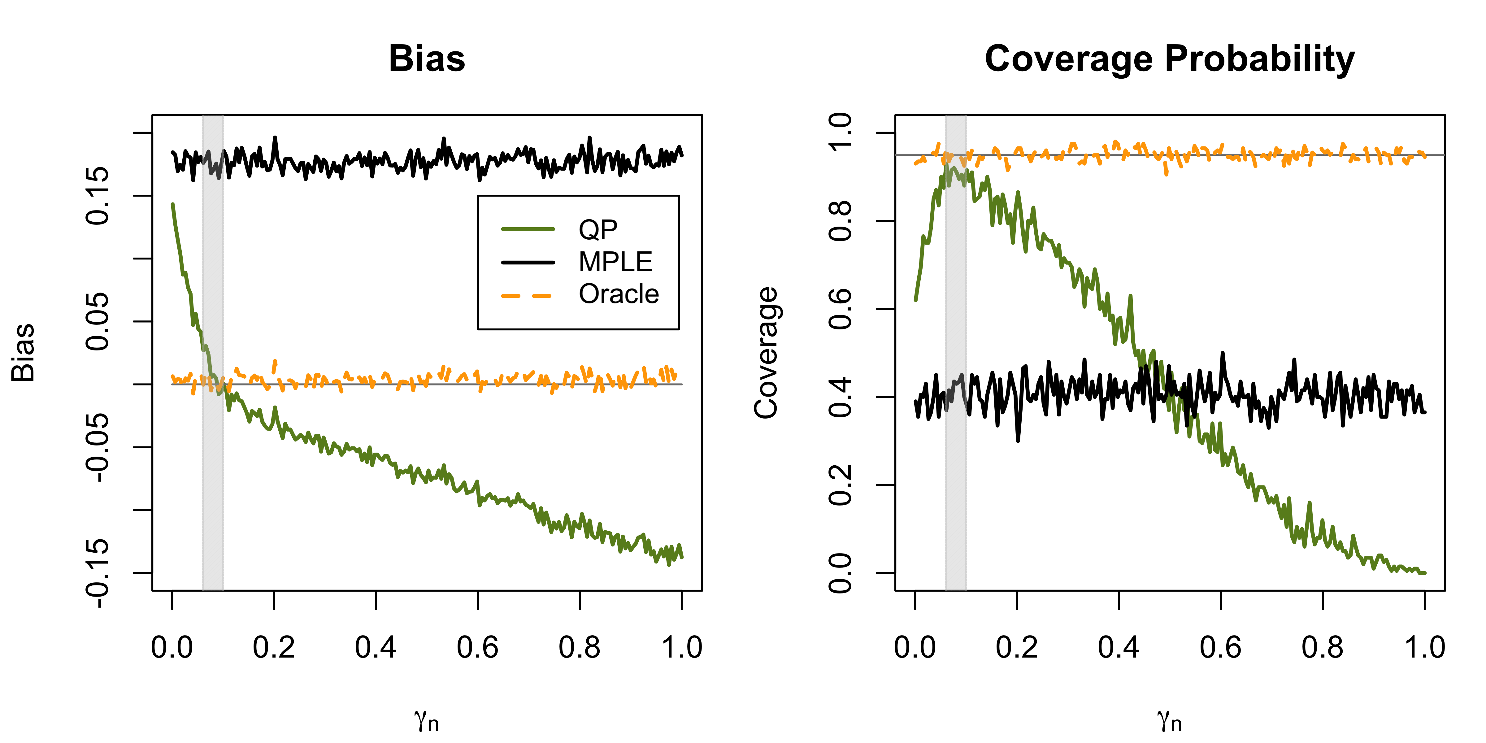
Figure 1: Estimation bias and 95% confidence interval coverage probability for $\beta_{1}^{0}=1$ with the tuning parameter $\gamma_{n}\in[0,1]$ in a simulated example with $n=500$ observations and $p=100$ independent covariates. The methods in comparison include the proposed debiased lasso with quadratic programming (QP), the maximum partial likelihood estimation (MPLE) and the oracle estimator (Oracle) obtained from fitting the true model.

We have found that, when evaluating cross-validation criteria for choosing $\gamma_{n}$, directly plugging in debiased estimates produces highly unstable values because of accumulative errors from inclusion of the estimates for a large number of noise covariates. Instead, we propose a cross-validation procedure by hard-thresholding debiased estimates: splitting data randomly into $K$ folds ($K=5$ or $10$), we use the $k$th fold to obtain a debiased lasso estimate $\widehat{b}^{(k)}$, hard-threshold it and plug in the thresholded values for computing cross-validation criteria. Hard-thresholding is based on multiple testing with, for example, the Bonferroni correction. That is, we take the hard-thresholded values to be $\widehat{b}^{(k),HT}_{j}=\widehat{b}^{(k)}_{j}$ if $\sqrt{n}|\widehat{b}^{(k)}_{j}|/\widehat{\Theta}_{jj}>z_{\alpha/(2p)}$, or $0$ otherwise, where $z_{\alpha/(2p)}$ is the upper $(\alpha/(2p))$th percentile of $N(0,1)$, as determined by the asymptotic result given in Theorem 1. Then, letting $\ell^{(k)}$ be the negative log partial likelihood [defined as in (1) but applied to the $k$th testing set] evaluated at $\widehat{b}^{(k),HT}$, we choose $\gamma_{n}$ that gives the smallest cross-validated negative partial likelihood, $\sum_{k=1}^{K}n^{(k)}\ell^{(k)}$, where $n^{(k)}$ is the number of observations in the $k$th testing set. Use of an alternative cross-validated partial likelihood (Verweij and van Houwelingen,, 1993) gives similar results.

3 Theoretical results

We infer $c^{T}\beta^{0}$ for a loading vector $c\in\mathbb{R}^{p}$ or $A\beta^{0}$ for a loading matrix $A\in\mathbb{R}^{l\times p}$, by studying the asymptotic properties for linear combinations of $\widehat{b}$. Denote the expectation of $\widehat{\mu}_{r}(t;\beta)$ as $\mu_{r}(t;\beta)=E[1(Y\geq t)X^{\otimes r}\exp\{X^{T}\beta\}]$, and define population-level counterparts for $\widehat{\eta}_{n}(t;\beta)$ as $\eta_{0}(t;\beta)=\mu_{1}(t;\beta)/\mu_{0}(t;\beta),$ and for $\widehat{\Sigma}$ in (4) as $\Sigma_{\beta^{0}}=E\left[\{X-\eta_{0}(Y;\beta^{0})\}^{\otimes 2}\delta\right].$ Denote by $\Theta_{\beta^{0}}=\Sigma_{\beta^{0}}^{-1}$. We enumerate sufficient conditions needed for establishing the theoretical properties of the debiased lasso estimator.

• Assumption 1. Covariates are almost surely uniformly bounded, i.e. $\|X_{i}\|_{\infty}\leq K$ for some constant $K<\infty$ for $i=1,2,\ldots,n$.

• Assumption 2. $|X_{i}^{T}\beta^{0}|\leq K_{1}$ uniformly for all $i=1,\cdots,n$ with some constant $K_{1}<\infty$ almost surely.

• Assumption 3. The follow-up time stops at a finite time point $\tau>0$, where the probability $\pi_{0}={P}(Y\geq\tau)>0$.

• Assumption 4. Let

  $$\widetilde{\Sigma}_{\beta^{0}}(t)=\int_{0}^{t}\left\{\mu_{2}(u;\beta^{0})-\frac{\mu_{1}(u;\beta^{0})\mu_{1}^{T}(u;\beta^{0})}{\mu_{0}(u;\beta^{0})}\right\}dH_{0}(u).$$

  For any $t\in[0,\tau]$, we assume

  $$\frac{c^{T}\Theta_{\beta^{0}}\widetilde{\Sigma}_{\beta^{0}}(t)\Theta_{\beta^{0}}c}{c^{T}\Theta_{\beta^{0}}c}\rightarrow v(t;c),~{}\mathrm{as}~{}n\rightarrow\infty$$

  for some fixed function $v(\cdot;c)>0$.

• Assumption 5. The matrix $\Sigma_{\beta^{0}}$ has bounded eigenvalues, i.e. there exist two constants $\zeta_{\mathrm{min}}$ and $\zeta_{\mathrm{max}}$ such that $0<\zeta_{\mathrm{min}}\leq\zeta_{\mathrm{min}}(\Sigma_{\beta^{0}})\leq\zeta_{\mathrm{max}}(\Sigma_{\beta^{0}})\leq\zeta_{\mathrm{max}}<\infty$, where $\zeta_{\mathrm{min}}(\Sigma_{\beta^{0}})$ and $\zeta_{\mathrm{max}}(\Sigma_{\beta^{0}})$ represent the smallest and the largest eigenvalues of $\Sigma_{\beta^{0}}$.

It is common in the literature of high-dimensional inference to assume bounded covariates as in Assumption 1. Fang et al., (2017) and Kong et al., (2018) also posed Assumption 2 for the Cox model inference, i.e. uniform boundedness on the multiplicative hazard. Under Assumption 1, Assumption 2 can be implied by bounded overall signal $\|\beta^{0}\|_{1}$. Assumption 3 is usually used for survival models with censored data (Andersen and Gill,, 1982). Assumption 4 ensures the convergence of a predictable variation process in the Martingale central limit theorem and thus the asymptotic normality of the de-biased lasso estimator. $\widetilde{\Sigma}_{\beta^{0}}(t)$ can be viewed as the information matrix up to time point $t$. It is easy to see that $\widetilde{\Sigma}_{\beta^{0}}(\tau)=\Sigma_{\beta^{0}}$ and $v(\tau;c)=1$. This assumption states that the limiting function $v(t;c)$ also depends on $c\in\mathbb{R}^{p}$, the loading vector of interest, which is reasonable. The bounded eigenvalue condition on $\Sigma_{\beta^{0}}$ in Assumption 5 is standard in inference for high-dimensional models.

Theorem 1.

Assume that the two tuning parameters satisfy $\lambda_{n}\asymp\sqrt{\log(p)/n}$ and $\gamma_{n}\asymp\|\Theta_{\beta^{0}}\|_{1,1}s_{0}\lambda_{n}$. Furthermore, assume $\|\Theta_{\beta^{0}}\|_{1,1}^{2}ps_{0}\log(p)/\sqrt{n}\rightarrow 0$ as $n\rightarrow\infty$. Under Assumptions 1–5, for any $c\in\mathbb{R}^{p}$ such that $\|c\|_{2}=1$ and $\|c\|_{1}\leq a_{*}$ with some absolute constant $a_{*}<\infty$, we have

$$\sqrt{n}c^{T}(\widehat{b}-\beta^{0})/(c^{T}\widehat{\Theta}c)^{1/2}\overset{\mathcal{D}}{\rightarrow}N(0,1).$$

Theorem 1 provides the foundation for drawing inference on the regression coefficients. In the following, Corollary 2(i) discusses the type I error and the power of testing $H_{0}:c^{T}\beta^{0}=a_{0}$ based on Theorem 1, and Corollary 2(ii) ensures that the corresponding confidence interval achieve nominal coverage probability asymptotically.

Corollary 2.

Suppose that the assumptions in Theorem 1 hold.

(i) To test a null hypothesis $H_{0}:c^{T}\beta^{0}=a_{0}$ versus an alternative hypothesis $H_{1}:c^{T}\beta^{0}=a_{1}$, where $a_{1}\neq a_{0}$, with a known $c\in\mathbb{R}^{p}$ and constant $a_{0}\in\mathbb{R}$, let the test statistic $T=\sqrt{n}(c^{T}\widehat{b}-a_{0})/(c^{T}\widehat{\Theta}c)^{1/2}$. We construct a test function

$$\phi(T)=\left\{\begin{array}[]{ll}1&\quad\mathrm{if}\ |T|>z_{\alpha/2}\\ 0&\quad\mathrm{if}\ |T|\leq z_{\alpha/2}\end{array},\right.$$

where $z_{\alpha/2}$ is the upper $(\alpha/2)$th quantile of $N(0,1)$. Then, the type I error rate for the test $\phi(T)$ satisfies ${P}(\phi(T)=1|H_{0})\to\alpha$, and the power under the alternative $H_{1}$ satisfies ${P}(\phi(T)=1|H_{1})\to 1$ as $n\to\infty$.

(ii) The two-sided level $\alpha$ confidence interval for $c^{T}\beta^{0}$ can be constructed as $CI(\alpha)=[c^{T}\widehat{b}-z_{\alpha/2}(c^{T}\widehat{\Theta}c/n)^{1/2},~{}c^{T}\widehat{b}+z_{\alpha/2}(c^{T}\widehat{\Theta}c/n)^{1/2}]$. Then ${P}(c^{T}\beta^{0}\in CI(\alpha)|H_{0})\rightarrow 1-\alpha$ as $n\rightarrow\infty$.

With Theorem 1 and the Cramér-Wold device, we can also conduct simultaneous inference on multiple linear combinations, i.e. $A\beta^{0}$ for some $l\times p$ matrix $A$, as summarized in the following Theorem 3, with Assumption 4 replaced by its multivariate version, Assumption 6. Similarly, Corollary 4 provides the asymptotic results for hypothesis testing and confidence region in this setting.

• Assumption 6. Let $\widetilde{\Sigma}_{\beta^{0}}(t)$ be the same as in Assumption 4. For a fixed combination matrix of interest $A\in\mathbb{R}^{l\times p}$, it holds that

  $$\frac{\omega^{T}A\Theta_{\beta^{0}}\widetilde{\Sigma}_{\beta^{0}}(t)\Theta_{\beta^{0}}A^{T}\omega}{\omega^{T}A\Theta_{\beta^{0}}A^{T}\omega}\rightarrow v^{\prime}(t;A^{T}\omega),~{}\mathrm{as}~{}n\rightarrow\infty$$

  for any vector $\omega\in\mathbb{R}^{l}$ and any $t\in[0,\tau]$, where $v^{\prime}(\cdot;A^{T}\omega)>0$ is some fixed function depending on $A^{T}\omega$.

Theorem 3.

Let $A$ be an $l\times p$ matrix of full row rank such that the number of rows $l$ is fixed, $\|A\|_{\infty,\infty}=\mathcal{O}(1)$ and $A\Theta_{\beta^{0}}A^{T}\rightarrow F$ for some fixed $l\times l$ matrix $F$. Assume that the two tuning parameters $\lambda_{n}\asymp\sqrt{\log(p)/n}$ and $\gamma_{n}\asymp\|\Theta_{\beta^{0}}\|_{1,1}s_{0}\lambda_{n}$, and that $\|\Theta_{\beta^{0}}\|_{1,1}^{2}ps_{0}\log(p)/\sqrt{n}\rightarrow 0$ as $n\rightarrow\infty$. Under Assumptions 1–3, 5 and 6, we have

$$\sqrt{n}A(\widehat{b}-\beta^{0})\overset{\mathcal{D}}{\rightarrow}N(0,F).$$

Corollary 4.

Suppose the assumptions in Theorem 3 hold.

(i) For the $l\times p$ matrix $A$ in Theorem 3, under the null hypothesis $H_{0}:A\beta^{0}=a_{0}$ for some $a_{0}\in\mathbb{R}^{l}$, the statistic $T^{\prime}=n(A\widehat{b}-a^{0})^{T}\widehat{F}^{-1}(A\widehat{b}-a^{0})\overset{\mathcal{D}}{\rightarrow}\chi^{2}_{l}$, where $\widehat{F}=A\widehat{\Theta}A^{T}$.

(ii) For $\alpha\in(0,1)$, let the confidence region for $A\beta^{0}$ be $CR(\alpha)=\{a\in\mathbb{R}^{l}:n(A\widehat{b}-a)^{T}\widehat{F}^{-1}(A\widehat{b}-a)\leq\chi^{2}_{l,\alpha}\}$, where $\chi^{2}_{l,\alpha}$ is the upper $\alpha$th percentile from $\chi^{2}_{l}$. Then ${P}(A\beta^{0}\in CR(\alpha)|H_{0})\rightarrow 1-\alpha$ as $n\rightarrow\infty$.

Proofs of Theorems 1 and 3 are provided in the Appendix. Corollaries 2 and 4 are directly obtained from Theorems 1 and 3, and their proofs are omitted.

4 Numerical experiments

For a total of $n=500$ subjects, we simulate $p=20,100,200$ covariates, respectively, and generate these covariates from $N(0,\Sigma)$, where $\Sigma=I_{p}$ and AR(1) with the correlation parameter of 0.5 as two different setups. Each covariate is truncated at $\pm 2.5$. Concerning the specifications of the true regression coefficients $\beta^{0}$, the first element $\beta_{1}^{0}$ varies from 0 to 2 with an equal step size of 0.2, four of the other elements are arbitrarily chosen to take values of 1, 1, 0.5 and 0.5, and the rest are set to be zero. The underlying survival times $T$ and the censoring times $C$ are independently generated from an exponential distribution with hazard $h(t|X)=\exp\{X^{T}\beta^{0}\}$, and from $\mathrm{Uniform}(1,20)$, respectively. Under each simulation configuration, 200 datasets are generated.

The methods in comparison include: (1) QP: our proposed debiased lasso with quadratic programming for matrix $\widehat{\Theta}$; (2) NW: the debiased lasso with node-wise lasso for matrix $\widehat{\Theta}$ in Kong et al., (2018); (3) CLIME: debiased lasso with CLIME for matrix $\widehat{\Theta}$ in Yu et al., (2018); (4) Decor: decorrelated Wald test in Fang et al., (2017) and (5) Oracle: the estimator when the true model is known a priori.

For the lasso estimator, we use 10-fold cross-validation to select the tuning parameter $\lambda_{n}$. Five-fold cross-validation is used for tuning parameter selection in CLIME, QP and NW. For the hard-thresholding step used to select $\gamma_{n}$ as described in Section 2.3, we adopt the Bonferroni correction with the adjusted p-value threshold $0.1/p$, where $p$ is the number of covariates.

We compare these methods with respect to the bias of the estimated $\beta^{0}_{1}$ (the parameter of main interest), its model-based standard error, coverage probability with a significance level of $\alpha=0.05$ and mean squared error. Figures 2 and 3 show the results for the independent and the AR(1) covariance structures, respectively. When $p=20$, our proposed method (QP) and the decorrelated Wald test (Decor) perform nearly as well as the oracle estimator (Oracle) and MPLE. When the dimension is relatively large compared to the sample size, i.e. $p=100,200$, next to Oracle, the proposed estimator (QP) displays the smallest biases and the confidence intervals with coverage probabilities closest to the nominal level 95% for both covariance structures. On the other hand, NW, CLIME, Decor and MPLE incur substantial biases as the true value of $\beta^{0}$ increases. In addition, owing to the estimation of $\Theta_{\beta^{0}}$ using penalized approaches, the model-based standard error estimates using NW and CLIME are shrunk towards zero, underestimating the true variation. As such, the four competing methods all present improper confidence interval coverage probabilities, whereas our proposed method retains nearly unbiased estimates with coverage probabilities close to the nominal level.

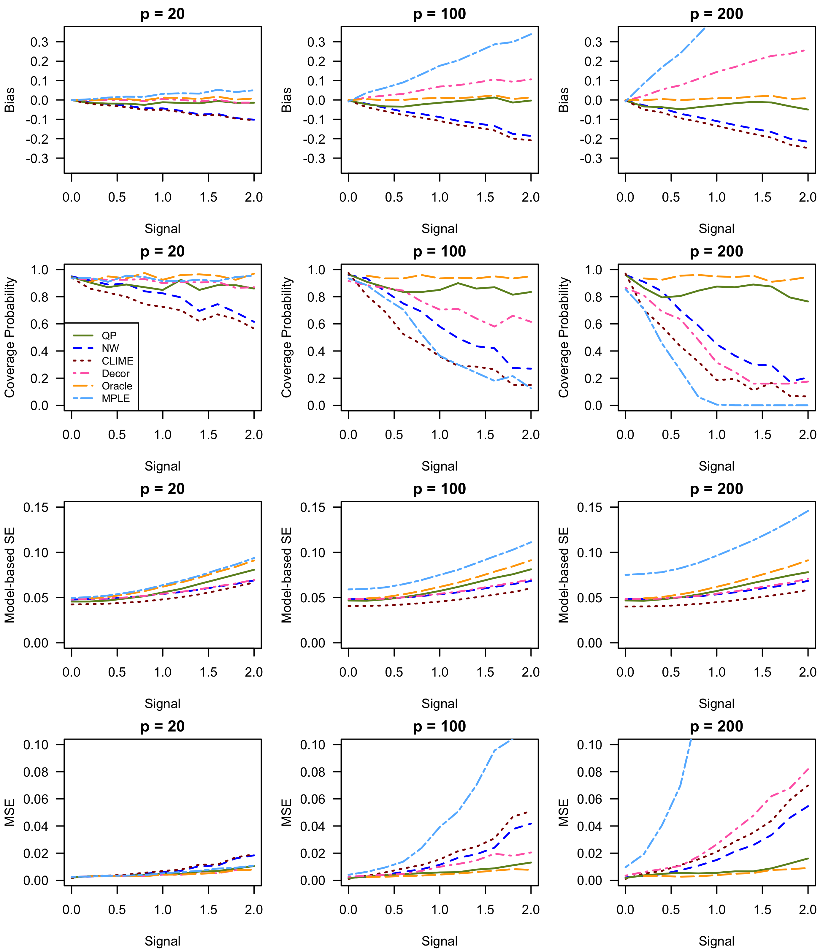
Figure 2: Estimation bias, coverage probability, model-based standard error and mean squared error for six estimators in comparison, QP (solid green lines), NW (short-dash navy blue lines), CLIME (dotted red lines), Decor (dot-dash pink lines), Oracle (long-dash orange lines), and MPLE (two-dash light blue lines), based on 200 simulations, each with $n=500$ observations and independent covariance structure for covariates.

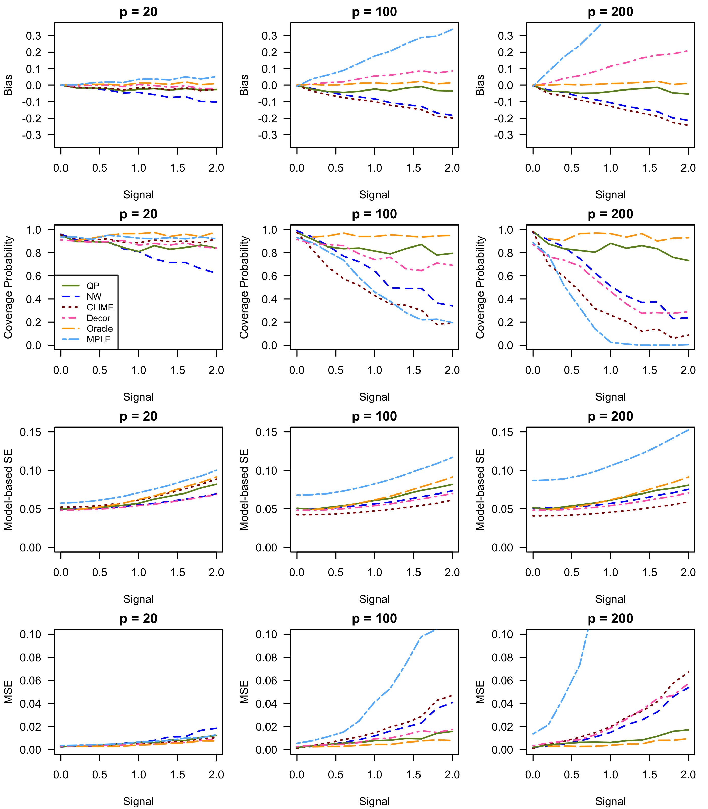
Figure 3: Estimation bias, coverage probability, model-based standard error and mean squared error for six estimators in comparison, QP (solid green lines), NW (short-dash navy blue lines), CLIME (dotted red lines), Decor (dot-dash pink lines), Oracle (long-dash orange lines), and MPLE (two-dash light blue lines), based on 200 simulations, each with $n=500$ observations and AR(1) covariance structure for covariates ($\rho=0.5$).

We next compare the time spent on computing $\widehat{\Theta}$ alone (Table 1) among solve.QP in the R package quadprog for the proposed quadratic programming procedure, and two commonly used R functions for CLIME, namely, clime in the package clime and sugm in the package flare. Three candidate values of $\gamma_{n}$, namely, 0.3, 1 and 2 times of $\sqrt{\log(p)/n}$, are used for demonstration. We fix $\beta^{0}_{1}=1$ and simulate $n=500$ observations, with covariates having an AR(1) covariance structure and the rest of the setting being identical to what is described in the first paragraph of this section. The time columns in Table 1 report the average computing time over 10 replications on a MacBook with 2.7GHz Intel Core i5 processor and 8GB memory, and the ratio columns compare the average computing time of each programming procedure to that of solve.QP for each simulation setting, respectively. Under all of the scenarios examined, our proposed implementation with solve.QP is the most computationally efficient; for large dimensions, e.g., $p=200$, clime takes the longest time per dataset on average.

Table 1: Comparison of the computational time spent on computing $\widehat{\Theta}$. Time (in seconds) is averaged over 10 replications under each setting. Time ratio is with respect to the proposed method implemented using solve.QP.

	solve.QP		clime		flare
$p=20$	Time	Ratio	Time	Ratio	Time	Ratio
$\gamma_{n}=0.3\sqrt{\log(p)/n}$	0.0016	1.0	0.0392	24.5	0.1898	118.6
$\gamma_{n}=\sqrt{\log(p)/n}$	0.0015	1.0	0.0373	24.9	0.1597	106.5
$\gamma_{n}=2\sqrt{\log(p)/n}$	0.0012	1.0	0.0338	28.2	0.1522	126.8
$p=100$	Time	Ratio	Time	Ratio	Time	Ratio
$\gamma_{n}=0.3\sqrt{\log(p)/n}$	0.3159	1.0	4.3452	13.8	5.8860	18.6
$\gamma_{n}=1\sqrt{\log(p)/n}$	0.0922	1.0	3.4164	37.1	2.0754	22.5
$\gamma_{n}=2\sqrt{\log(p)/n}$	0.0665	1.0	2.6281	39.5	0.3663	5.5
$p=200$	Time	Ratio	Time	Ratio	Time	Ratio
$\gamma_{n}=0.3\sqrt{\log(p)/n}$	4.3886	1.0	64.7047	14.7	52.2224	11.9
$\gamma_{n}=1\sqrt{\log(p)/n}$	0.9039	1.0	47.0320	52.0	21.7229	24.0
$\gamma_{n}=2\sqrt{\log(p)/n}$	0.6196	1.0	33.0308	53.3	2.5536	4.1

5 Boston lung cancer data analysis

Lung cancer is the leading cause of cancer deaths in the United States, and non-small cell lung cancer (NSCLC), accounting for approximately 80% to 85% among all the lung cancer cases, is the most common histological type of lung cancer (Houston et al.,, 2018). Identification of genetic variants associated with lung cancer patient survival sparks modern translational cancer research, and has the potential to refine prognosis and promote individualized treatment and clinical care. Despite numerous studies investigating potential predisposing genes to lung cancer risks, studies on patient survival usually have small sample sizes and the reported genetic markers associated with lung cancer survival have been poorly replicated (Bossé and Amos,, 2018). The Boston Lung Cancer Survival Cohort (BLCSC) is a large epidemiology cohort for investigating the molecular cause underlying lung cancer, where lung cancer cases have been enrolled at Massachusetts General Hospital and the Dana-Farber Cancer Institute from 1992 to present. We apply the proposed debiased lasso method (QP) to a BLCSC cohort with genetic data and simultaneously investigate the joint effects of certain genotyped SNPs on NSCLC patient overall survival.

Included in the analysis are $n=561$ NSCLC patients with available diagnosis dates, follow-up times and genotypes on Axiom arrays. Among all these patients, 437 (77.9%) died and 124 (22.1%) were censored. The range of the observed survival time is from 6 days to $8584$ days, and the restricted mean survival and censoring times at $\tau=8584$ days are 2124 (SE: 105) and 4397 (SE: 187) days, respectively. Patient characteristics, including age at diagnosis, race, education level, gender, smoking status, histological type, cancer stage, and treatment received, are provided in the online supplementary materials.

A conventional marginal association analysis (Tang et al.,, 2020) found two potentially functional SNPs in the genes HDAC2 and PPARGC1A that were significantly associated with NSCLC overall survival. Using the target gene approach, we focus on 32 genes in the CARM ER pathway, which is the largest pathway Tang et al., (2020) considered and described in their supplementary document and contains the two reported genes HDAC2 and PPARGC1A, plus 9 genes that Xia et al., (2020) studied to investigate whether the susceptibility loci are also associated with patient survival. We extract 312 genotyped SNPs from the 32 genes in the CARM ER pathway and the nine target genes described in Xia et al., (2020) from the BLCSC data (minor allele frequency $>$ 0.01, genotype call rate $>$ 95%). After a pruning step using PLINK (Purcell et al.,, 2007) to avoid multicolinearity caused by SNPs with high linkage disequilibrium, the number of SNPs is reduced to 217. SNPs are coded by the number of copies of the minor allele, i.e. 0, 1 or 2, and assumed to have additive effects on the log hazard ratio. Therefore, the subset of the BLCSC data we analyze include $n=561$ NSCLC patients and $p=231$ covariates.

Table 2 summarizes the coefficient estimates in the Cox proportional hazards model for all patient characteristics and the top ten SNPs ranked by the p-values from the proposed method (QP). Results of two methods, QP versus MPLE, are listed side by side. In general, QP results in points estimates of smaller magnitudes and smaller standard errors compared to MPLE, which is consistent with our observation in the simulated example. MPLE is numerically very unstable when the dimension $p$ is large compared to the sample size $n$. The numerical instability arises primarily from inverting the Hessian matrix, which may be closer to being singular. On the contrary, Lasso provides a more stabilized initial estimator. As a result, the debiased lasso estimator is numerically more stable than MPLE with narrower confidence intervals. When the dimension $p$ is very small, the difference between the two methods becomes negligible.

Table 2: Coefficient estimates in the Cox proportional hazards model for the Boston Lung Cancer Study data

			QP				MPLE
Variable	Note		Est	SE	P-value	95% CI	Est	SE	P-value	95% CI
Race	Others vs Caucasian		-0.163	0.201	0.416	(-0.557, 0.231)	0.065	0.561	0.908	(-1.034, 1.163)
Education	HS vs No HS		-0.018	0.091	0.840	(-0.198, 0.161)	-0.142	0.253	0.574	(-0.637, 0.353)
	College vs No HS		-0.037	0.076	0.625	(-0.185, 0.111)	-0.085	0.218	0.698	(-0.513, 0.343)
Gender	Male vs Female		0.314	0.075	$<0.001$	(0.166, 0.461)	0.439	0.166	0.008	(0.114, 0.763)
Age	Standardized		0.155	0.038	$<0.001$	(0.081, 0.230)	0.400	0.090	$<0.001$	(0.224, 0.577)
Smoker	Yes vs No		0.103	0.142	0.470	(-0.176, 0.381)	0.066	0.299	0.825	(-0.519, 0.651)
Histology	AD vs LCC		-0.259	0.076	0.001	(-0.409, -0.11)	-0.467	0.294	0.112	(-1.043, 0.109)
	SCC vs LCC		0.065	0.094	0.488	(-0.120, 0.251)	-0.030	0.314	0.923	(-0.646, 0.585)
	Unspecified vs LCC		0.046	0.132	0.729	(-0.213, 0.304)	-0.119	0.384	0.756	(-0.871, 0.633)
Stage	Late vs Early		0.352	0.081	$<0.001$	(0.193, 0.510)	0.553	0.190	0.004	(0.180, 0.926)
Surgery	Yes vs No		-1.102	0.085	$<0.001$	(-1.269, -0.936)	-2.115	0.226	$<0.001$	(-2.557, -1.672)
Chemotherapy	Yes vs No		0.025	0.078	0.753	(-0.128, 0.177)	-0.239	0.220	0.278	(-0.671, 0.193)
Radiation	Yes vs No		0.047	0.077	0.548	(-0.105, 0.198)	0.248	0.198	0.211	(-0.140, 0.636)
Treatment record	Missing vs Not		0.099	0.176	0.573	(-0.245, 0.443)	0.347	0.428	0.417	(-0.492, 1.186)
SNP	Pos	Gene	Est	SE	P-value	95% CI	Est	SE	P-value	95% CI
AX-11672686	8:27324822	CHRNA2	0.186	0.054	0.001	(0.081, 0.291)	0.185	0.402	0.645	(-0.603, 0.973)
AX-11673610	12:66762242	GRIP1	0.313	0.092	0.001	(0.133, 0.494)	0.773	0.220	$<0.001$	(0.343, 1.203)
AX-11264571	13:32906729	BRCA2	0.206	0.061	0.001	(0.086, 0.325)	0.450	0.164	0.006	(0.129, 0.772)
AX-40031129	16:3860539	CREBBP	-0.566	0.242	0.019	(-1.040, -0.092)	-1.504	0.623	0.016	(-2.726, -0.282)
AX-11235551	16:3832471	CREBBP	-0.130	0.057	0.022	(-0.242, -0.019)	-0.495	0.309	0.110	(-1.101, 0.112)
AX-11639833	5:88088439	MEF2C	-0.121	0.056	0.031	(-0.231, -0.011)	-0.145	0.120	0.228	(-0.381, 0.091)
AX-11326149	15:78867482	CHRNA5	0.102	0.051	0.046	(0.002, 0.202)	1.273	0.366	0.001	(0.555, 1.991)
AX-11376755	21:16340289	NRIP1	-0.101	0.052	0.052	(-0.202, 0.001)	-0.281	0.120	0.019	(-0.516, -0.046)
AX-40181207	17:41218805	BRCA1	-0.524	0.272	0.054	(-1.056, 0.009)	-2.386	0.750	0.001	(-3.856, -0.916)
AX-30854303	12:66761377	GRIP1	0.094	0.054	0.081	(-0.011, 0.199)	0.102	0.117	0.380	(-0.126, 0.331)
$\vdots$

• Est: coefficient estimate; SE: standard error estimate; CI: confidence interval; HS: high school; AD: Adenocarcinoma; SCC: squamous cell carcinoma; LCC: large cell carcinoma; Pos: physical location based on Assembly GRCh37/hg19.

Among various patient characteristics, QP found that the adenocarcinoma subtype is significantly associated with better patient survival than large cell carcinoma, consistent with the results of Janssen-Heijnen and Coebergh, (2001), which was, however, not detected by MPLE. QP further identified that AX-11672686 in CHRNA2, AX-11673610 in GRIP2 and AX-11264571 in BRCA2 are the three most significant SNPs associated with NSCLC patient survival, after adjusting for all the other demographic and genetic risk factors. Interestingly, AX-11672686 was found to be associated with nicotine dependence by Wang et al., (2014). AX-11264571 has been found to be associated with breast cancer (Qiu et al.,, 2010) and may also be associated with lung cancer susceptibility, although not achieving genome-wide significance in Yu et al., (2011). AX-11673610 or GRIP1 seems to be a new finding as, to our knowledge, they have yet been reported in the lung cancer literature (Bossé and Amos,, 2018)

To understand the impact of the socioeconomic status on cancer survival, we test for the association between education level (no high school, high school, or at least 1–2 years of college) and lung cancer patient survival. With a loading matrix $A_{2\times p}=(e_{2},e_{3})^{T}$ corresponding to the contrast of the effects of high school graduate and at least 1–2 years of college with the reference level of no high school, the test statistic is 0.259 with a p-value of 0.879, suggesting no statistical evidence for the association between education level and NSCLC patient survival, after adjusting all other demographic characteristics and genetic markers. The results confirm a large-scale clinical trial on lung cancer patients which reported “education level was not predictive of survival” (Herndon et al.,, 2008).

In summary, these results illustrate the utility of our method in providing reliable inference for scientific discovery and interpretation, while more in-depth biological investigations are warranted to validate our findings.

6 Concluding remarks

We have proposed a debiased lasso approach for reliable estimation and inference in the Cox proportional hazards model when $p<n$ but is allowed to diverge to $\infty$ with $n$. Unlike existing methods (Fang et al.,, 2017; Yu et al.,, 2018; Kong et al.,, 2018), we resort a quadratic programming procedure to estimate the inverse information matrix, without imposing an unrealistic sparsity assumption on it. The proposed debiased lasso estimator is asymptotically unbiased and normally distributed under mild regularity conditions. Our simulations demonstrate that, when $p$ is very small, the proposed method behaves similarly to the conventional MPLE; when $p$ is relatively large, it outperforms the competitors in bias correction and confidence interval coverage.

Lastly, we touch upon the important issue of drawing inference with $p>n$, though not a main focus of this paper. First, several methods (Fang et al.,, 2017; Yu et al.,, 2018; Kong et al.,, 2018) had been developed for handling “$p>n$” inference problems; however, our analytical and simulation studies have pinpointed their possible limitations in providing sufficient bias correction and reliable confidence intervals even within the “large $n$, diverging $p$” framework, likely due to the sparsity assumptions on the inverse information matrix that may not hold in survival settings. One possible solution, by going beyond the de-biased lasso framework, is to perform repeated data splitting for model selection and estimation on two separate parts of the data and smooth the resulting estimates from multiple splits; see Fei and Li, (2021) for inference on high dimensional generalized linear models. The validity of the method hinges upon the sure screening property for the initial model selection, and we will explore its use in a survival setting in the future.

Appendix

We first present the useful lemmas for proving the main theorems, with detailed proofs deferred to the online supplementary materials. Some of these lemmas present important results in their own right. The proofs of the Theorem 1 and Theorem 3 are presented following the lemmas.

Additional notation from counting processes and martingale theory is defined for the proofs. Under the Cox model, define the counting process $N_{i}(t)=1(Y_{i}\leq t,\delta_{i}=1)$ and its compensator $A_{i}(t;\beta)=\int_{0}^{t}1(Y_{i}\geq s)\exp(X_{i}^{T}\beta)dH_{0}(s)$, where $H_{0}(t)=\int_{0}^{t}h_{0}(s)ds$ is the cumulative baseline hazard function, $i=1,\cdots,n$. Let $M_{i}(t;\beta)=N_{i}(t)-A_{i}(t;\beta)$, and $M_{i}(t;\beta^{0})$ is a martingale with respect to the filtration $\mathcal{F}_{i}(t)=\sigma\{N_{i}(s),1(Y_{i}\geq s),X_{i}:s\in(0,t]\}$. It follows that $\widehat{\eta}_{n}(t;{\beta)}$, and in particular, $\widehat{\eta}_{n}(t;{\beta^{0})}$, is predictable with respect to the filtration $\mathcal{F}(t)=\sigma\{N_{i}(s),1(Y_{i}\geq s),X_{i}:s\in(0,t],i=1,\cdots,n\}$, an observation useful for derivations. Notation-wise, we do not distinguish between the usual expectation and the outer expectation.

Lemma A1 below characterizes the difference between $\widehat{\eta}_{n}(t;\beta^{0})$ and $\eta_{0}(t;\beta^{0})$, which facilitates the proof of the asymptotic distribution for the leading term $\sqrt{n}c^{T}\Theta_{\beta^{0}}\dot{\ell}_{n}(\beta^{0})$ as well as the establishment of the convergence rate for $\widehat{\Sigma}-\Sigma_{\beta^{0}}$.

Lemma A1.

Under Assumptions 1–3, we have

$$\sup_{t\in[0,\tau]}|\widehat{\mu}_{0}(t;\beta^{0})-\mu_{0}(t;\beta^{0})|=\mathcal{O}_{P}(\sqrt{\log(p)/n}),$$

$$\sup_{t\in[0,\tau]}\|\widehat{\mu}_{1}(t;\beta^{0})-\mu_{1}(t;\beta^{0})\|_{\infty}=\mathcal{O}_{P}(\sqrt{\log(p)/n}),$$

$$\sup_{t\in[0,\tau]}\|\widehat{\eta}_{n}(t;\beta^{0})-\eta_{0}(t;\beta^{0})\|_{\infty}=\mathcal{O}_{P}(\sqrt{\log(p)/n}).$$

Lemma A2 establishes the asymptotic distribution for the leading term $-c^{T}\Theta_{\beta^{0}}\dot{\ell}_{n}(\beta^{0})$ in the decomposition of $c^{T}(\widehat{b}-\beta^{0})$.

Lemma A2.

Assume $p^{2}\log(p)/n\rightarrow 0$. Under Assumptions 1–5, for any $c\in\mathbb{R}^{p}$ such that $\|c\|_{2}=1$ and $\|c\|_{1}\leq a_{*}$ with some absolute constant $a_{*}<\infty$,

$$\frac{\sqrt{n}c^{T}\Theta_{\beta^{0}}\dot{\ell}_{n}(\beta^{0})}{\sqrt{c^{T}\Theta_{\beta^{0}}c}}\overset{\mathcal{D}}{\rightarrow}N(0,1).$$

Lemma A3 provides theoretical properties of the lasso estimator in the Cox model. This is a direct result from Theorem 1 in Kong and Nan, (2014), and thus the proof is omitted.

Lemma A3.

Under Assumptions 1–5, for the lasso estimator $\widehat{\beta}$, we have

$$\|\widehat{\beta}-\beta^{0}\|_{1}=\mathcal{O}_{P}(s_{0}\lambda_{n}),\quad\frac{1}{n}\sum_{i=1}^{n}|X_{i}^{T}(\widehat{\beta}-\beta^{0})|^{2}=\mathcal{O}_{P}(s_{0}\lambda_{n}^{2}),$$

where $s_{0}=|\{j:\beta_{j}^{0}\neq 0,j=1,\cdots,p\}|$ is the true model size.

Lemma A4.

Under Assumptions 1–5, if $\lambda_{n}\asymp\sqrt{\log(p)/n}$, with probability going to 1, we have $\|\Theta_{\beta^{0}}\widehat{\Sigma}-I_{p}\|_{\infty}\leq\gamma_{n}$, for $\gamma_{n}\asymp\|\Theta_{\beta^{0}}\|_{1,1}s_{0}\lambda_{n}$.

Lemma A4 shows that, unlike in a linear regression model where the tuning parameter in the constraint takes the order of $\sqrt{\log(p)/n}$, the Cox model requires a potentially larger $\gamma_{n}$ for the feasibility of $\Theta_{\beta^{0}}$ depending on $\|\Theta_{\beta^{0}}\|_{1,1}$, because the information matrix involves the regression coefficients.

Lemma A5.

Assume $\limsup_{n\rightarrow\infty}p\gamma_{n}\leq 1-\epsilon^{\prime}$ for some $\epsilon^{\prime}\in(0,1)$. Then, under the assumptions in Lemma A4, $\|\widehat{\Theta}-\Theta_{\beta^{0}}\|_{\infty}=\mathcal{O}_{P}(\gamma_{n}\|\Theta_{\beta^{0}}\|_{1,1})$.

Lemma A6.

Under Assumptions 1–3 and 5, for each $t>0$,

$${P}\left(\|\dot{\ell}_{n}(\beta^{0})\|_{\infty}>t\right)\leq 2pe^{-nt^{2}/(8K^{2})}.$$

Now we complete the proofs of Theorem 1 and Theorem 3.

Proof of Theorem 1..

The first order Taylor expansion of $\dot{\ell}_{nj}(\widehat{\beta})$, the $j$th component in $\dot{\ell}_{n}(\widehat{\beta})$, at $\beta^{0}$, is

$$\dot{\ell}_{nj}(\widehat{\beta})=\dot{\ell}_{nj}(\beta^{0})+[\ddot{\ell}_{nj}(\widetilde{\beta}^{(j)})]^{T}(\widehat{\beta}-\beta^{0}),$$ (A1)

where $\widetilde{\beta}^{(j)}$ lies between $\widehat{\beta}$ and $\beta^{0}$, and $\ddot{\ell}_{nj}(\beta)$ denotes the $j$th column in the Hessian matrix $\ddot{\ell}_{n}(\beta)$. Let the $p\times p$ matrix $B_{n}=(\ddot{\ell}_{n1}(\widetilde{\beta}^{(1)}),\ldots,\ddot{\ell}_{np}(\widetilde{\beta}^{(p)}))^{T}$. Suppose $c\in\mathbb{R}^{p}$ is a $p$-dimensional vector, and the parameter of interest is $c^{T}\beta^{0}$. Plugging (A1) in (2), we have

$$c^{T}(\widehat{b}-\beta^{0}) =-c^{T}\Theta_{\beta^{0}}\dot{\ell}_{n}(\beta^{0})-c^{T}(\widehat{\Theta}-\Theta_{\beta^{0}})\dot{\ell}_{n}(\beta^{0})$$

$$\quad-c^{T}(\widehat{\Theta}\widehat{\Sigma}-I_{p})(\widehat{\beta}-\beta^{0})+c^{T}\widehat{\Theta}(\widehat{\Sigma}-B_{n})(\widehat{\beta}-\beta^{0}).$$ (A2)

The first term in (Proof of Theorem 1..) is the leading part and is asymptotically normal as shown in Lemma A2, and the others will be proved to be asymptotically negligible.

First, we show that $\sqrt{n}c^{T}(\widehat{\Theta}-\Theta_{\beta^{0}})\dot{\ell}_{n}(\beta^{0})=o_{P}(1)$. By Lemma A5 and Lemma A6,

$$|\sqrt{n}c^{T}(\widehat{\Theta}-\Theta_{\beta^{0}})\dot{\ell}_{n}(\beta^{0})| \leq\sqrt{n}\|c\|_{1}\cdot\|\widehat{\Theta}-\Theta_{\beta^{0}}\|_{\infty,\infty}\cdot\|\dot{\ell}_{n}(\beta^{0})\|_{\infty}$$

$$\leq\sqrt{n}a_{*}\mathcal{O}_{P}(p\gamma_{n}\|\Theta_{\beta^{0}}\|_{1,1})\mathcal{O}_{P}(\sqrt{\log(p)/n})$$

$$=\mathcal{O}_{P}(\|\Theta_{\beta^{0}}\|_{1,1}p\gamma_{n}\sqrt{\log(p)})$$

$$=o_{P}(1).$$

Second, we show that $\sqrt{n}c^{T}(\widehat{\Theta}\widehat{\Sigma}-I_{p})(\widehat{\beta}-\beta^{0})=o_{P}(1)$. By Lemma A3,

$$|\sqrt{n}c^{T}(\widehat{\Theta}\widehat{\Sigma}-I_{p})(\widehat{\beta}-\beta^{0})| \leq\sqrt{n}\|c\|_{1}\|(\widehat{\Theta}\widehat{\Sigma}-I_{p})(\widehat{\beta}-\beta^{0})\|_{\infty}$$

$$\leq\sqrt{n}a_{*}\|\widehat{\Theta}\widehat{\Sigma}-I_{p}\|_{\infty}\|\widehat{\beta}-\beta^{0}\|_{1}$$

$$\leq\sqrt{n}a_{*}\gamma_{n}\|\widehat{\beta}-\beta^{0}\|_{1}$$

$$=\mathcal{O}_{P}(\sqrt{n}\gamma_{n}s_{0}\lambda_{n})$$

$$=o_{P}(1).$$

Next, we show that $\sqrt{n}c^{T}\widehat{\Theta}(\widehat{\Sigma}-B_{n})(\widehat{\beta}-\beta^{0})=o_{P}(1)$. Note that

$$\widehat{\Sigma}-B_{n}=(\widehat{\Sigma}-\Sigma_{\beta^{0}})+(\Sigma_{\beta^{0}}-\ddot{\ell}_{n}(\beta^{0}))+(\ddot{\ell}_{n}(\beta^{0})-B_{n}).$$ (A3)

By the proof of Lemma A4, we see that with $\lambda_{n}\asymp\sqrt{\log(p)/n}$, $\|\widehat{\Sigma}-\Sigma_{\beta^{0}}\|_{\infty}=\mathcal{O}_{P}(s_{0}\lambda_{n})$. We rewrite

$$\Sigma_{\beta^{0}}-\ddot{\ell}_{n}(\beta^{0}) =\displaystyle\mathbb{E}\int^{\tau}_{0}\{X_{i}-\eta_{0}(t;\beta^{0})\}^{\otimes 2}e^{X_{i}^{T}\beta^{0}}1(Y_{i}\geq t)h_{0}(t)dt$$

$$\quad-\int_{0}^{\tau}\left\{\widehat{\mu}_{2}(t;\beta^{0})-\frac{\widehat{\mu}_{1}(t;\beta^{0})\widehat{\mu}_{1}^{T}(t;\beta^{0})}{\widehat{\mu}_{0}(t;\beta^{0})}\right\}h_{0}(t)dt$$

$$\quad-\frac{1}{n}\sum_{i=1}^{n}\int_{0}^{\tau}\left\{\frac{\widehat{\mu}_{2}(t;\beta^{0})}{\widehat{\mu}_{0}(t;\beta^{0})}-\left[\frac{\widehat{\mu}_{1}(t;\beta^{0})}{\widehat{\mu}_{0}(t;\beta^{0})}\right]^{\otimes 2}\right\}dM_{i}(t)$$

$$=\int_{0}^{\tau}\{\mu_{2}(t;\beta^{0})-\widehat{\mu}_{2}(t;\beta^{0})\}h_{0}(t)dt$$

$$\quad+\int_{0}^{\tau}\left\{\frac{\widehat{\mu}_{1}(t;\beta^{0})\widehat{\mu}_{1}^{T}(t;\beta^{0})}{\widehat{\mu}_{0}(t;\beta^{0})}-\frac{\mu_{1}(t;\beta^{0})\mu_{1}^{T}(t;\beta^{0})}{\mu_{0}(t;\beta^{0})}\right\}h_{0}(t)dt$$

$$\quad-\frac{1}{n}\sum_{i=1}^{n}\int_{0}^{\tau}\left\{\frac{\widehat{\mu}_{2}(t;\beta^{0})}{\widehat{\mu}_{0}(t;\beta^{0})}-\left[\frac{\widehat{\mu}_{1}(t;\beta^{0})}{\widehat{\mu}_{0}(t;\beta^{0})}\right]^{\otimes 2}\right\}dM_{i}(t).$$ (A4)

Similar to the proof in Lemma A1, we can show that $\sup_{t\in[0,\tau]}\|\widehat{\mu}_{2}(t;\beta^{0})-\mu_{2}(t;\beta^{0})\|_{\infty}=\mathcal{O}_{P}(\sqrt{\log(p)/n})$, and thus $\|\int_{0}^{\tau}\{\mu_{2}(t;\beta^{0})-\widehat{\mu}_{2}(t;\beta^{0})\}h_{0}(t)dt\|_{\infty}\leq\sup_{t\in[0,\tau]}\|\widehat{\mu}_{2}(t;\beta^{0})-\mu_{2}(t;\beta^{0})\|_{\infty}\int_{0}^{\tau}h_{0}(t)dt=\mathcal{O}_{P}(\sqrt{\log(p)/n})$. Since

$$\frac{\widehat{\mu}_{1}\widehat{\mu}_{1}^{T}}{\widehat{\mu}_{0}}-\frac{\mu_{1}\mu_{1}^{T}}{\mu_{0}}=\frac{\widehat{\mu}_{1}\widehat{\mu}_{1}^{T}}{\widehat{\mu}_{0}\mu_{0}}(\mu_{0}-\widehat{\mu}_{0})+\frac{1}{\mu_{0}}[(\widehat{\mu}_{1}-\mu_{1})\widehat{\mu}_{1}^{T}+\mu_{1}(\widehat{\mu}_{1}-\mu_{1})^{T}]$$

in the second term of (A4), by Assumption 1 and Lemma A1,

$$\left\|\int_{0}^{\tau}\left\{\frac{\widehat{\mu}_{1}(t;\beta^{0})\widehat{\mu}_{1}^{T}(t;\beta^{0})}{\widehat{\mu}_{0}(t;\beta^{0})}-\frac{\mu_{1}(t;\beta^{0})\mu_{1}^{T}(t;\beta^{0})}{\mu_{0}(t;\beta^{0})}\right\}h_{0}(t)dt\right\|_{\infty}=\mathcal{O}_{P}(\sqrt{\log(p)/n}).$$

$n^{-1}\sum_{i=1}^{n}\int_{0}^{\tau}\left\{{\mu_{2}(t;\beta^{0})}/{\mu_{0}(t;\beta^{0})}-\left[{\mu_{1}(t;\beta^{0})}/{\mu_{0}(t;\beta^{0})}\right]^{\otimes 2}\right\}dM_{i}(t)$ is a sum of $n$ independent and identically distributed mean zero terms, and each term $\left\|\int_{0}^{\tau}\left\{{\mu_{2}(t;\beta^{0})}/{\mu_{0}(t;\beta^{0})}-\left[{\mu_{1}(t;\beta^{0})}/{\mu_{0}(t;\beta^{0})}\right]^{\otimes 2}\right\}dM_{i}(t)\right\|_{\infty}$ is bounded by $2K^{2}(1+e^{K_{1}}H_{0}(\tau))$ uniformly for all $i$ and $t\in[0,\tau]$. Similar to the proof of $\|A_{n}\|_{\infty}=\mathcal{O}_{P}(\sqrt{\log(p)/n})$ in Lemma A4, by Hoeffding’s concentration inequality,

$$\left\|\displaystyle\frac{1}{n}\sum_{i=1}^{n}\int_{0}^{\tau}\left\{\frac{\mu_{2}(t;\beta^{0})}{\mu_{0}(t;\beta^{0})}-\left[\frac{\mu_{1}(t;\beta^{0})}{\mu_{0}(t;\beta^{0})}\right]^{\otimes 2}\right\}dM_{i}(t)\right\|_{\infty}=\mathcal{O}_{P}(\sqrt{\log(p)/n}).$$

It is easy to see that

$$\sup_{t\in[0,\tau]}\left\|\left\{\frac{\widehat{\mu}_{2}(t;\beta^{0})}{\widehat{\mu}_{0}(t;\beta^{0})}-\left[\frac{\widehat{\mu}_{1}(t;\beta^{0})}{\widehat{\mu}_{0}(t;\beta^{0})}\right]^{\otimes 2}\right\}-\left\{\frac{\mu_{2}(t;\beta^{0})}{\mu_{0}(t;\beta^{0})}-\left[\frac{\mu_{1}(t;\beta^{0})}{\mu_{0}(t;\beta^{0})}\right]^{\otimes 2}\right\}\right\|_{\infty}=\mathcal{O}_{P}\left(\sqrt{\displaystyle\frac{\log(p)}{n}}\right).$$

Then

$$\left\|\frac{1}{n}\sum_{i=1}^{n}\int_{0}^{\tau}\left\{\frac{\widehat{\mu}_{2}(t;\beta^{0})}{\widehat{\mu}_{0}(t;\beta^{0})}-\left[\frac{\widehat{\mu}_{1}(t;\beta^{0})}{\widehat{\mu}_{0}(t;\beta^{0})}\right]^{\otimes 2}\right\}dM_{i}(t)\right.$$

$$\left.-\frac{1}{n}\sum_{i=1}^{n}\int_{0}^{\tau}\left\{\frac{\mu_{2}(t;\beta^{0})}{\mu_{0}(t;\beta^{0})}-\left[\frac{\mu_{1}(t;\beta^{0})}{\mu_{0}(t;\beta^{0})}\right]^{\otimes 2}\right\}dM_{i}(t)\right\|_{\infty}=\mathcal{O}_{P}\left(\sqrt{\displaystyle\frac{\log(p)}{n}}\right),$$

and thus for the third term in (A4),

$$\left\|\frac{1}{n}\sum_{i=1}^{n}\int_{0}^{\tau}\left\{\frac{\widehat{\mu}_{2}(t;\beta^{0})}{\widehat{\mu}_{0}(t;\beta^{0})}-\left[\frac{\widehat{\mu}_{1}(t;\beta^{0})}{\widehat{\mu}_{0}(t;\beta^{0})}\right]^{\otimes 2}\right\}dM_{i}(t)\right\|_{\infty}=\mathcal{O}_{P}(\sqrt{\log(p)/n}).$$

Therefore, by (A4), $\|\Sigma_{\beta^{0}}-\ddot{\ell}_{n}(\beta^{0})\|_{\infty}=\mathcal{O}_{P}(\sqrt{\log(p)/n})$.

For the $(j,k)$th element in $\ddot{\ell}_{n}(\beta)$, denoted as $\ddot{\ell}_{njk}(\beta)$, by the mean value theorem, we have

$$\ddot{\ell}_{njk}(\widetilde{\beta}^{(j)})-\ddot{\ell}_{njk}(\beta^{0})=\displaystyle(\widetilde{\beta}^{(j)}-\beta^{0})^{T}\left.\frac{\partial\ddot{\ell}_{njk}(\beta)}{\partial\beta}\right|_{\beta=\overline{\beta}^{(jk)}},$$

where $\overline{\beta}^{(jk)}$ lies in the segment between $\widetilde{\beta}^{(j)}$ and $\beta^{0}$. Under Assumptions 1–3, when $\|\beta-\beta^{0}\|_{1}\leq\delta^{\prime}$ for $\delta^{\prime}>0$ small enough, $\left\|{\partial\ddot{\ell}_{njk}(\beta)}/{\partial\beta}\right\|_{\infty}$ is bounded by some constant related to $\delta^{\prime}$ uniformly for all $(j,k)$. Since $s_{0}\lambda_{n}=o(1)$, we have $\|B_{n}-\ddot{\ell}_{n}(\beta^{0})\|_{\infty}\leq\mathcal{O}_{P}(\|\widehat{\beta}-\beta^{0}\|_{1})=\mathcal{O}_{P}(s_{0}\lambda_{n})$.

Combining the three parts in (A3), we have that for $\lambda_{n}\asymp\sqrt{\log(p)/n}$, $\|\widehat{\Sigma}-B_{n}\|_{\infty}=\mathcal{O}_{P}(s_{0}\lambda_{n})$. Then

$$|\sqrt{n}c^{T}\widehat{\Theta}(\widehat{\Sigma}-B_{n})(\widehat{\beta}-\beta^{0})| \leq\sqrt{n}\|c\|_{1}\|\widehat{\Theta}\|_{\infty,\infty}\|\widehat{\Sigma}-B_{n}\|_{\infty}\|\widehat{\beta}-\beta^{0}\|_{1}$$

$$\leq\mathcal{O}_{P}(\sqrt{n}\|\Theta_{\beta^{0}}\|_{1,1}(s_{0}\lambda_{n})^{2})$$

$$=o_{P}(1).$$

We show that the variance estimator is consistent, i.e. $c^{T}(\widehat{\Theta}-\Theta_{\beta^{0}})c\rightarrow_{P}0$ as $n\rightarrow\infty$.

$$|c^{T}(\widehat{\Theta}-\Theta_{\beta^{0}})c| \leq\|c\|_{1}^{2}\|\widehat{\Theta}-\Theta_{\beta^{0}}\|_{\infty}$$

$$\leq a_{*}^{2}\mathcal{O}_{P}(\gamma_{n}\|\Theta_{\beta^{0}}\|_{1,1})=o_{P}(1).$$

Finally, by the arguments above and Slutsky’s theorem, it holds that $\sqrt{n}c^{T}(\widehat{b}-\beta^{0})/(c^{T}\widehat{\Theta}c)^{1/2}\overset{\mathcal{D}}{\rightarrow}N(0,1)$. ∎

Proof of Theorem 3..

We prove Theorem 3 using the Cramér-Wold device. For any $\omega\in\mathbb{R}^{l}$, where the dimension $l$ is a fixed integer free of $n$ and $p$, let $c=A^{T}\omega$ in Theorem 1. Essentially, we only require $\|c\|_{1}=\|A^{T}\omega\|_{1}$ is upper bounded, and it is not essential to force $\|c\|_{2}=1$. Since $\|A\|_{\infty,\infty}=\mathcal{O}(1)$ (by assumption) and $\|\omega\|_{1}=\mathcal{O}(1)$ (fixed $l$), then $\|A^{T}\omega\|_{1}\leq\|A^{T}\|_{1,1}\|\omega\|_{1}=\|A\|_{\infty,\infty}\|\omega\|_{1}=\mathcal{O}(1).$ ∎

Supplementary Materials for “Statistical Inference for Cox Proportional Hazards Models with a Diverging Number of Covariates”

We provide detailed proofs for the lemmas presented in the Appendix of the article, as well as patient characteristics of the Boston Lung Cancer Study Cohort data analyzed in Section 5.

S1 Technical proofs for the lemmas

Lemma A1 characterizes the difference between $\widehat{\eta}_{n}(t;\beta^{0})$ and $\eta_{0}(t;\beta^{0})$, which is needed to prove the asymptotic distribution for the leading term $\sqrt{n}c^{T}\Theta_{\beta^{0}}\dot{\ell}_{n}(\beta^{0})$ as well as to establish the convergence rate for $\widehat{\Sigma}-\Sigma_{\beta^{0}}$.

Lemma A1.

Under Assumptions 1–3, we have

$$\sup_{t\in[0,\tau]}|\widehat{\mu}_{0}(t;\beta^{0})-\mu_{0}(t;\beta^{0})|=\mathcal{O}_{P}(\sqrt{\log(p)/n}),$$

$$\sup_{t\in[0,\tau]}\|\widehat{\mu}_{1}(t;\beta^{0})-\mu_{1}(t;\beta^{0})\|_{\infty}=\mathcal{O}_{P}(\sqrt{\log(p)/n}),$$

$$\sup_{t\in[0,\tau]}\|\widehat{\eta}_{n}(t;\beta^{0})-\eta_{0}(t;\beta^{0})\|_{\infty}=\mathcal{O}_{P}(\sqrt{\log(p)/n}).$$

Proof of Lemma A1.

The first two statements in the conclusion are similar to those in Kong and Nan, (2014), but with differing setups. Consider a class of functions of $y\geq 0$ and $x\in\mathbb{R}^{p}$ indexed by $t$, $\mathcal{F}_{0}=\{1(y\geq t)\exp(x^{T}\beta^{0}):t\in[0,\tau]\}$. For any $0<\epsilon<1$, consider the cumulative distribution function for $Y$ and take an positive integer $m<2/\epsilon$ and a sequence of points $0=t_{0}<t_{1}<\cdots<t_{m-1}<t_{m}=\infty$ such that ${P}(t_{i}<Y\leq t_{i+1})<\epsilon,~{}i=0,1,\ldots,m-1$. For each $i=1,\cdots,m$, define the bracket $[L_{i},U_{i}]$, where $L_{i}(x,y)=1(y\geq t_{i})\exp(x^{T}\beta^{0})$ and $U_{i}(x,y)=1(y>t_{i-1})\exp(x^{T}\beta^{0})$. We have $L_{i}(x,y)\leq 1(y\geq t)\exp(x^{T}\beta^{0})\leq U_{i}(x,y)$ for $t_{i-1}<t\leq t_{i}$, and

$$[\mathbb{E}\{U_{i}(X,Y)-L_{i}(X,Y)\}^{2}]^{1/2}=[\mathbb{E}\{1(t_{i-1}<Y<t_{i})\exp(2X^{T}\beta^{0})\}]^{1/2}\leq e^{K_{1}}\sqrt{\epsilon},$$

$$\mathbb{E}|U_{i}(X,Y)-L_{i}(X,Y)|=\mathbb{E}\{1(t_{i-1}<Y<t_{i})\exp(X^{T}\beta^{0})\}\leq e^{K_{1}}\epsilon.$$

Then the bracketing numbers van der Vaart, (1998) satisfy

$$N_{[]}(e^{K_{1}}\sqrt{\epsilon},\mathcal{F}_{0},L_{2}({P}))\leq\frac{2}{\epsilon},\quad N_{[]}(e^{K_{1}}{\epsilon},\mathcal{F}_{0},L_{1}({P}))\leq\frac{2}{\epsilon},$$

or equivalently,

$$N_{[]}(\epsilon,\mathcal{F}_{0},L_{2}({P}))\leq\frac{2e^{2K_{1}}}{\epsilon^{2}},\quad N_{[]}({\epsilon},\mathcal{F}_{0},L_{1}({P}))\leq\frac{2e^{K_{1}}}{\epsilon}<\infty.$$

By the Glivenko-Cantelli Theorem and the Donsker Theorem (van der Vaart,, 1998), the class of $\mathcal{F}_{0}$ is ${P}$-Glivenko-Cantelli and ${P}$-Donsker. So $\sup_{t\in[0,\tau]}|\widehat{\mu}_{0}(t;\beta^{0})-\mu_{0}(t;\beta^{0})|\overset{a.s.}{\rightarrow}0$, and moreover, by Theorem 2.14.9 of van der Vaart and Wellner, (1996) with $V=2$,

$${P}\left(\sqrt{n}\sup_{t\in[0,\tau]}|\widehat{\mu}_{0}(t;\beta^{0})-\mu_{0}(t;\beta^{0})|>s\right)\leq De^{-s^{2}},$$

for every $s>0$ and a constant $D>0$ that only depends on $K_{1}$. Setting $s=\sqrt{2\log(p)}$ implies that

$$\sup_{t\in[0,\tau]}|\widehat{\mu}_{0}(t;\beta^{0})-\mu_{0}(t;\beta^{0})|=\mathcal{O}_{P}(\sqrt{\log(p)/n}).$$

For the second statement, we consider the classes of functions of $(x,y)=(x_{1},\cdots,x_{p},y)$ indexed by $t$,

$$\mathcal{F}_{1}^{k}=\{1(y\geq t)e^{x^{T}\beta^{0}}x_{k}:t\in[0,\tau]\},~{}k=1,\cdots,p.$$

Since $|e^{x^{T}\beta^{0}}x_{k}|\leq Ke^{K_{1}}$, similarly we have

$$N_{[]}(\epsilon,\mathcal{F}_{1}^{k},L_{2}({P}))\leq\left(\frac{\sqrt{2}e^{K_{1}}K}{\epsilon}\right)^{2}.$$

By Theorem 2.14.9 of van der Vaart and Wellner, (1996) with $V=2$, we have

$${P}\left(\sqrt{n}\sup_{t\in[0,\tau]}|\widehat{\mu}_{1k}(t;\beta^{0})-\mu_{1k}(t;\beta^{0})|>s\right)\leq D^{\prime}s^{2}e^{-2s^{2}}\leq D^{\prime}e^{-1}e^{-s^{2}}$$

for every $s>0$, where $D^{\prime}$ is a constant that only depends on $K$ and $K_{1}$, and $\widehat{\mu}_{1k}$ and $\mu_{1k}$ are the $k$th components of $\widehat{\mu}_{1}$ and $\mu_{1}$, respectively. Thus,

$${P}\left(\sqrt{n}\sup_{t\in[0,\tau]}\|\widehat{\mu}_{1}(t;\beta^{0})-\mu_{1}(t;\beta^{0})\|_{\infty}>s\right)$$

$$\leq ~{}{P}\left(\bigcup_{k=1}^{p}\left\{\sqrt{n}\sup_{t\in[0,\tau]}|\widehat{\mu}_{1k}(t;\beta^{0})-\mu_{1k}(t;\beta^{0})|>s\right\}\right)$$

$$\leq ~{}pD^{\prime}e^{-s^{2}}.$$

For example, taking $s=\sqrt{2\log(p)}$ would complete the proof for $\sup_{t\in[0,\tau]}\|\widehat{\mu}_{1}(t;\beta^{0})-\mu_{1}(t;\beta^{0})\|_{\infty}=\mathcal{O}_{P}(\sqrt{\log(p)/n})$.

Finally, we rewrite

$$\widehat{\eta}_{n}(t;\beta^{0})-\eta_{0}(t;\beta^{0}) =\displaystyle\frac{\widehat{\mu}_{1}(t;\beta^{0})}{\widehat{\mu}_{0}(t;\beta^{0})}-\frac{\mu_{1}(t;\beta^{0})}{\mu_{0}(t;\beta^{0})}$$

$$=\displaystyle\frac{\widehat{\mu}_{1}(t;\beta^{0})}{\mu_{0}(t;\beta^{0})}-\frac{\mu_{1}(t;\beta^{0})}{\mu_{0}(t;\beta^{0})}+\frac{\widehat{\mu}_{1}(t;\beta^{0})}{\mu_{0}(t;\beta^{0})}\left(\displaystyle\frac{\mu_{0}(t;\beta^{0})}{\widehat{\mu}_{0}(t;\beta^{0})}-1\right).$$

By Assumptions 1–3, $\mu_{0}(t;\beta^{0})\geq e^{-K_{1}}\pi_{0}>0$ and $\sup_{t\in[0,\tau]}\|\widehat{\mu}_{1}(t;\beta^{0})\|_{\infty}=\mathcal{O}_{P}(1)$. Also, since

$$\inf_{t\in[0,\tau]}\widehat{\mu}_{0}(t;\beta^{0})\geq\mu_{0}(t;\beta^{0})-|\widehat{\mu}_{0}(t;\beta^{0})-\mu_{0}(t;\beta^{0})|\geq e^{-K_{1}}\pi_{0}-\sup_{t\in[0,\tau]}|\widehat{\mu}_{0}(t;\beta^{0})-\mu_{0}(t;\beta^{0})|>e^{-K_{1}}\frac{\pi_{0}}{2}$$

almost surely, we have

$$\sup_{t\in[0,\tau]}\left\|\frac{\widehat{\mu}_{1}(t;\beta^{0})}{\mu_{0}(t;\beta^{0})}\left(\frac{\mu_{0}(t;\beta^{0})}{\widehat{\mu}_{0}(t;\beta^{0})}-1\right)\right\|_{\infty}$$

$$\leq ~{}\sup_{t\in[0,\tau]}\left\|\frac{\widehat{\mu}_{1}(t;\beta^{0})}{\mu_{0}(t;\beta^{0})}\right\|_{\infty}\cdot\sup_{t\in[0,\tau]}\left|\frac{\mu_{0}(t;\beta^{0})}{\widehat{\mu}_{0}(t;\beta^{0})}-1\right|$$

$$\leq ~{}\mathcal{O}_{P}(1)\sup_{t\in[0,\tau]}\left|\mu_{0}(t;\beta^{0})-\widehat{\mu}_{0}(t;\beta^{0})\right|=\mathcal{O}_{P}(\sqrt{\log(p)/n}).$$

Therefore,

$$\sup_{t\in[0,\tau]}\|\widehat{\eta}_{n}(t;\beta^{0})-\eta_{0}(t;\beta^{0})\|_{\infty} \leq\sup_{t\in[0,\tau]}\left\|\displaystyle\frac{1}{\mu_{0}(t;\beta^{0})}\left(\widehat{\mu}_{1}(t;\beta^{0})-\mu_{1}(t;\beta^{0})\right)\right\|_{\infty}$$

$$\quad+\sup_{t\in[0,\tau]}\left\|\frac{\widehat{\mu}_{1}(t;\beta^{0})}{\mu_{0}(t;\beta^{0})}\left(\frac{\mu_{0}(t;\beta^{0})}{\widehat{\mu}_{0}(t;\beta^{0})}-1\right)\right\|_{\infty}$$

$$=\mathcal{O}_{P}(\sqrt{\log(p)/n}).$$

∎

Lemma A2 establishes the asymptotic distribution for the leading term $-c^{T}\Theta_{\beta^{0}}\dot{\ell}_{n}(\beta^{0})$ in the decomposition of $c^{T}(\widehat{b}-\beta^{0})$.

Lemma A2.

Assume $p^{2}\log(p)/n\rightarrow 0$. Under Assumptions 1–5, for any $c\in\mathbb{R}^{p}$ such that $\|c\|_{2}=1$ and $\|c\|_{1}\leq a_{*}$ with some absolute constant $a_{*}>0$,

$$\frac{\sqrt{n}c^{T}\Theta_{\beta^{0}}\dot{\ell}_{n}(\beta^{0})}{\sqrt{c^{T}\Theta_{\beta^{0}}c}}\overset{\mathcal{D}}{\rightarrow}N(0,1).$$

Proof of Lemma A2.

Using notation of martingales, we rewrite

$$\displaystyle\frac{-\sqrt{n}c^{T}\Theta_{\beta^{0}}\dot{\ell}_{n}(\beta^{0})}{\sqrt{c^{T}\Theta_{\beta^{0}}c}} =\displaystyle\frac{1}{\sqrt{n}}\sum_{i=1}^{n}\frac{c^{T}\Theta_{\beta^{0}}}{\sqrt{c^{T}\Theta_{\beta^{0}}c}}\left\{X_{i}-\frac{\widehat{\mu}_{1}(Y_{i};\beta^{0})}{\widehat{\mu}_{0}(Y_{i};\beta^{0})}\right\}\delta_{i}$$

$$=\displaystyle\frac{1}{\sqrt{n}}\sum_{i=1}^{n}\int_{0}^{\tau}\frac{c^{T}\Theta_{\beta^{0}}}{\sqrt{c^{T}\Theta_{\beta^{0}}c}}\left\{X_{i}-\frac{\widehat{\mu}_{1}(t;\beta^{0})}{\widehat{\mu}_{0}(t;\beta^{0})}\right\}dN_{i}(t)$$

$$=\displaystyle\frac{1}{\sqrt{n}}\sum_{i=1}^{n}\int_{0}^{\tau}\frac{c^{T}\Theta_{\beta^{0}}}{\sqrt{c^{T}\Theta_{\beta^{0}}c}}\left\{X_{i}-\frac{\widehat{\mu}_{1}(t;\beta^{0})}{\widehat{\mu}_{0}(t;\beta^{0})}\right\}dM_{i}(t).$$

Let $Q_{i}(t)=\displaystyle\frac{1}{\sqrt{n}}\frac{c^{T}\Theta_{\beta^{0}}}{\sqrt{c^{T}\Theta_{\beta^{0}}c}}\left\{X_{i}-\frac{\widehat{\mu}_{1}(t;\beta^{0})}{\widehat{\mu}_{0}(t;\beta^{0})}\right\},~{}i=1,\ldots,n$, which are predictable with respect to the filtration $\mathcal{F}$. Then

$$\frac{-\sqrt{n}c^{T}\Theta_{\beta^{0}}\dot{\ell}_{n}(\beta^{0})}{\sqrt{c^{T}\Theta_{\beta^{0}}c}}=\sum_{i=1}^{n}\int_{0}^{\tau}Q_{i}(t)dM_{i}(t).$$ (S1)

For any $t\in[0,\tau]$, let $U(t)=\sum_{i=1}^{n}\int_{0}^{t}Q_{i}(u)dM_{i}(u)$, whose predictable variation process is

$$\langle U\rangle(t) =\sum_{i=1}^{n}\int_{0}^{t}Q_{i}(u)^{2}1(Y_{i}\geq u)e^{X_{i}^{T}\beta^{0}}dH_{0}(u)$$

$$=\sum_{i=1}^{n}\int_{0}^{t}\frac{c^{T}\Theta_{\beta^{0}}}{c^{T}\Theta_{\beta^{0}}c}\left\{X_{i}-\frac{\widehat{\mu}_{1}(t;\beta^{0})}{\widehat{\mu}_{0}(t;\beta^{0})}\right\}^{\otimes 2}\Theta_{\beta^{0}}c1(Y_{i}\geq u)e^{X_{i}^{T}\beta^{0}}dH_{0}(u)$$

$$=\frac{c^{T}\Theta_{\beta^{0}}}{c^{T}\Theta_{\beta^{0}}c}\left[\int_{0}^{t}\left\{\widehat{\mu}_{2}(u;\beta^{0})-\frac{\widehat{\mu}_{1}(u;\beta^{0})\widehat{\mu}_{1}(u;\beta^{0})^{T}}{\widehat{\mu}_{0}(u;\beta^{0})}\right\}dH_{0}(u)\right]\Theta_{\beta^{0}}c$$

Similar to the proof in Lemma A1, we can show that $\sup_{t\in[0,\tau]}\|\widehat{\mu}_{2}(t;\beta^{0})-\mu_{2}(t;\beta^{0})\|_{\infty}=\mathcal{O}_{P}(\sqrt{\log(p)/n})$, and thus

$$\left\|\int_{0}^{t}\{\mu_{2}(u;\beta^{0})-\widehat{\mu}_{2}(u;\beta^{0})\}h_{0}(u)du\right\|_{\infty} \leq\sup_{u\in[0,\tau]}\|\widehat{\mu}_{2}(u;\beta^{0})-\mu_{2}(u;\beta^{0})\|_{\infty}\int_{0}^{\tau}h_{0}(u)du$$

$$=\mathcal{O}_{P}(\sqrt{\log(p)/n}).$$ (S2)

Since

$$\frac{\widehat{\mu}_{1}\widehat{\mu}_{1}^{T}}{\widehat{\mu}_{0}}-\frac{\mu_{1}\mu_{1}^{T}}{\mu_{0}}=\frac{\widehat{\mu}_{1}\widehat{\mu}_{1}^{T}}{\widehat{\mu}_{0}\mu_{0}}(\mu_{0}-\widehat{\mu}_{0})+\frac{1}{\mu_{0}}[(\widehat{\mu}_{1}-\mu_{1})\widehat{\mu}_{1}^{T}+\mu_{1}(\widehat{\mu}_{1}-\mu_{1})^{T}],$$

by Assumption 1 and Lemma A1,

$$\left\|\int_{0}^{t}\left\{\frac{\widehat{\mu}_{1}(u;\beta^{0})\widehat{\mu}_{1}^{T}(u;\beta^{0})}{\widehat{\mu}_{0}(u;\beta^{0})}-\frac{\mu_{1}(u;\beta^{0})\mu_{1}^{T}(u;\beta^{0})}{\mu_{0}(u;\beta^{0})}\right\}h_{0}(u)du\right\|_{\infty}=\mathcal{O}_{P}(\sqrt{\log(p)/n}).$$ (S3)

Combining (S1) and (S3), we have that, uniformly for all $t\in[0,\tau]$,

$$\left\|\int_{0}^{t}\left\{\widehat{\mu}_{2}(u;\beta^{0})-\frac{\widehat{\mu}_{1}(u;\beta^{0})\widehat{\mu}_{1}(u;\beta^{0})^{T}}{\widehat{\mu}_{0}(u;\beta^{0})}\right\}dH_{0}(u)-\right.$$

$$\quad\left.\int_{0}^{t}\left\{\mu_{2}(u;\beta^{0})-\frac{\mu_{1}(u;\beta^{0})\mu_{1}(u;\beta^{0})^{T}}{\mu_{0}(u;\beta^{0})}\right\}dH_{0}(u)\right\|_{\infty} =\mathcal{O}_{P}(\sqrt{\log(p)/n}).$$

Then

$$\left|\langle U\rangle(t)-\frac{c^{T}\Theta_{\beta^{0}}}{c^{T}\Theta_{\beta^{0}}c}\left[\int_{0}^{t}\left\{\mu_{2}(u;\beta^{0})-\frac{\mu_{1}(u;\beta^{0})\mu_{1}(u;\beta^{0})^{T}}{\mu_{0}(u;\beta^{0})}\right\}dH_{0}(u)\right]\Theta_{\beta^{0}}c\right|$$

$$\leq \zeta_{\mathrm{min}}^{-1}(\|c\|_{1}\|\Theta_{\beta^{0}}\|_{1,1})^{2}\mathcal{O}_{P}(\sqrt{\log(p)/n})$$

$$\leq \zeta_{\mathrm{min}}^{-1}a_{*}^{2}p\zeta_{\mathrm{max}}^{2}\mathcal{O}_{P}(\sqrt{\log(p)/n})\rightarrow_{P}0$$

if $p^{2}\log(p)/n\rightarrow 0$. By Assumption 4, $\langle U(t)\rangle\rightarrow_{P}v(t;c)$.

Now we check the Lindeberg condition. For any $\epsilon>0$, define the truncated process

$$U_{\epsilon}(t)=\sum_{i=1}^{n}\int_{0}^{t}Q_{i}(u)1\{|Q_{i}(u)|>\epsilon\}dM_{i}(u),$$

with a predictable variation process:

$$\langle U_{\epsilon}\rangle(t) =\sum_{i=1}^{n}\int_{0}^{t}Q_{i}^{2}(u)1\{|Q_{i}(u)|>\epsilon\}1(Y_{i}\geq u)e^{X_{i}^{T}\beta^{0}}h_{0}(u)du$$

$$=\sum_{i=1}^{n}\int_{0}^{t}Q_{i}^{2}(u)1\{|\sqrt{n}Q_{i}(u)|>\sqrt{n}\epsilon\}1(Y_{i}\geq u)e^{X_{i}^{T}\beta^{0}}h_{0}(u)du.$$

Let $Q_{\mathrm{max}}=\sup_{t\in[0,\tau]}\max_{1\leq i\leq n}|\sqrt{n}Q_{i}(t)|$, then $1\{|\sqrt{n}Q_{i}(u)|>\sqrt{n}\epsilon\}\leq 1\{Q_{\mathrm{max}}>\sqrt{n}\epsilon\}$. By Assumption 1,

$$\sup_{t\in[0,\tau]}\max_{1\leq i\leq n}\left|\displaystyle\frac{c^{T}\Theta_{\beta^{0}}}{\sqrt{c^{T}\Theta_{\beta^{0}}c}}\left\{X_{i}-\frac{\widehat{\mu}_{1}(t;\beta^{0})}{\widehat{\mu}_{0}(t;\beta^{0})}\right\}\right|\leq\zeta_{\mathrm{min}}^{-1/2}\|c\|_{1}\|\Theta_{\beta^{0}}\|_{1,1}2K=\mathcal{O}(\sqrt{p}),$$

and $Q_{\mathrm{max}}=\mathcal{O}(\sqrt{p})$. When $p/n\rightarrow 0$, $1\{Q_{\mathrm{max}}>\sqrt{n}\epsilon\}=0$ almost surely. Thus $\langle U_{\epsilon}\rangle(t)\rightarrow_{P}0$. Finally, by the martingale central limit theorem, the asymptotic normality follows. ∎

Lemma A3 provides the theoretical properties of the lasso estimator in the Cox model. This is a direct result from Theorem 1 in Kong and Nan, (2014), and thus the proof is omitted.

Lemma A3.

Under Assumptions 1–5, for the lasso estimator $\widehat{\beta}$, we have

$$\|\widehat{\beta}-\beta^{0}\|_{1}=\mathcal{O}_{P}(s_{0}\lambda_{n}),\quad\frac{1}{n}\sum_{i=1}^{n}|X_{i}^{T}(\widehat{\beta}-\beta^{0})|^{2}=\mathcal{O}_{P}(s_{0}\lambda_{n}^{2}),$$

where $s_{0}=|\{j:\beta_{j}^{0}\neq 0,j=1,\cdots,p\}|$ is the true model size.

Lemma A4.

Under Assumptions 1–5, if $\lambda_{n}\asymp\sqrt{\log(p)/n}$, with probability going to 1, we have $\|\Theta_{\beta^{0}}\widehat{\Sigma}-I_{p}\|_{\infty}\leq\gamma_{n}$, for $\gamma_{n}\asymp\|\Theta_{\beta^{0}}\|_{1,1}s_{0}\lambda_{n}$.

Lemma A4 shows that, unlike linear models with the tuning parameter in the constraint taking the order of $\sqrt{\log(p)/n}$, the Cox model requires a potentially larger $\gamma_{n}$ for the feasibility of $\Theta_{\beta^{0}}$ that depends on $\|\Theta_{\beta^{0}}\|_{1,1}$, as the information matrix involves the regression coefficients.

Proof of Lemma A4.

Write $A_{n}=\displaystyle\frac{1}{n}\sum_{i=1}^{n}\int_{0}^{\tau}\left\{X_{i}-\eta_{0}(t;\beta^{0})\right\}^{\otimes 2}dN_{i}(t)-\Sigma_{\beta^{0}}$.

$$\|\widehat{\Sigma}-\Sigma_{\beta^{0}}\|_{\infty} \leq\left\|\displaystyle\frac{1}{n}\sum_{i=1}^{n}\int_{0}^{\tau}\left[\left\{X_{i}-\widehat{\eta}_{n}(t;\widehat{\beta})\right\}^{\otimes 2}-\left\{X_{i}-\eta_{0}(t;\beta^{0})\right\}^{\otimes 2}\right]dN_{i}(t)\right\|_{\infty}$$

$$\quad+\left\|\displaystyle\frac{1}{n}\sum_{i=1}^{n}\int_{0}^{\tau}\left\{X_{i}-\eta_{0}(t;\beta^{0})\right\}^{\otimes 2}dN_{i}(t)-\Sigma_{\beta^{0}}\right\|_{\infty}$$

$$\leq\left\|\displaystyle\frac{1}{n}\sum_{i=1}^{n}\int_{0}^{\tau}\left\{X_{i}-\widehat{\eta}_{n}(t;\widehat{\beta})\right\}\left\{\widehat{\eta}_{n}(t;\widehat{\beta})-\eta_{0}(t;\beta^{0})\right\}^{T}dN_{i}(t)\right\|_{\infty}$$

$$\quad+\left\|\displaystyle\frac{1}{n}\sum_{i=1}^{n}\int_{0}^{\tau}\left\{\widehat{\eta}_{n}(t;\widehat{\beta})-\eta_{0}(t;\beta^{0})\right\}\left\{X_{i}-\eta_{0}(t;\beta^{0})\right\}^{T}dN_{i}(t)\right\|_{\infty}+\left\|A_{n}\right\|_{\infty}.$$

Note that for all $t\in[0,\tau]$, $\|X_{i}-\widehat{\eta}_{n}(t;\hat{\beta})\|_{\infty}\leq 2K$ and $\|X_{i}-{\eta}_{0}(t;\beta^{0})\|_{\infty}\leq 2K$. Then

$$\|\widehat{\Sigma}-\Sigma_{\beta^{0}}\|_{\infty} \leq\displaystyle\frac{4K}{n}\sum_{i=1}^{n}\int_{0}^{\tau}\|\widehat{\eta}_{n}(t;\hat{\beta})-\eta_{0}(t;\beta^{0})\|_{\infty}dN_{i}(t)+\|A_{n}\|_{\infty}$$

$$\leq\displaystyle\frac{4K}{n}\sum_{i=1}^{n}\int_{0}^{\tau}\|\widehat{\eta}_{n}(t;\hat{\beta})-\widehat{\eta}_{n}(t;\beta^{0})\|_{\infty}dN_{i}(t)$$

$$\quad+\displaystyle\frac{4K}{n}\sum_{i=1}^{n}\int_{0}^{\tau}\|\widehat{\eta}_{n}(t;{\beta^{0}})-\eta_{0}(t;\beta^{0})\|_{\infty}dN_{i}(t)+\|A_{n}\|_{\infty}.$$ (S4)

By the mean value theorem, for the $j$th component in $\widehat{\eta}_{n}$ (denoted by $\widehat{\eta}_{nj}$), there exists some $\bar{\beta}^{(j)}$ lying inside the segments connecting $\widehat{\beta}$ and $\beta^{0}$ such that

$$\widehat{\eta}_{nj}(t;\widehat{\beta})=\widehat{\eta}_{nj}(t;\beta^{0})+\left[\displaystyle\left.\frac{\partial\widehat{\eta}_{nj}(t;\beta)}{\partial\beta}\right|_{\beta=\bar{\beta}^{(j)}}\right]^{T}(\widehat{\beta}-\beta^{0}).$$

Consider $\beta$ in a neighborhood of $\beta^{0}$, i.e. when $\|\beta-\beta^{0}\|_{1}\leq\delta^{\prime}$ for some $\delta^{\prime}>0$, $e^{X_{i}^{T}\beta}\leq e^{|X_{i}^{T}\beta|}\leq e^{|X_{i}^{T}\beta^{0}|+K\delta^{\prime}}\leq e^{K_{1}+K\delta^{\prime}}$, and $e^{X_{i}^{T}\beta}\geq e^{-|X_{i}^{T}\beta|}\geq e^{-K_{1}-K\delta^{\prime}}$. Since $\{1(Y\geq t):t\in[0,\tau]\}$ is ${P}$-Glivenko-Cantelli, $\sup_{t\in[0,\tau]}|\frac{1}{n}\sum_{i=1}^{n}1(Y\geq t)-{P}(Y\geq t)|\overset{a.s.}{\rightarrow}0$, and then uniformly for $t\in[0,\tau]$ and $\beta\in\{\beta:\|\beta-\beta^{0}\|_{1}\leq\delta^{\prime}\}$,

$$\widehat{\mu}_{0}(t;\beta)\geq\frac{1}{n}\sum_{i=1}^{n}1(Y_{i}\geq t)e^{-K_{1}-K\delta^{\prime}}\overset{a.s.}{\rightarrow}{P}(Y\geq t)e^{-K_{1}-K\delta^{\prime}}\geq\frac{\pi_{0}}{2}e^{-K_{1}-K\delta^{\prime}}.$$

In this case, uniformly for $t\in[0,\tau]$ and $\beta\in\{\beta:\|\beta-\beta^{0}\|_{1}\leq\delta^{\prime}\}$,

$$\left\|\displaystyle\frac{\partial\widehat{\eta}_{n}(t;\beta)}{\partial\beta^{T}}\right\|_{\infty} =\left\|\displaystyle\frac{\widehat{\mu}_{2}(t;\beta)\widehat{\mu}_{0}(t;\beta)-\widehat{\mu}_{1}(t;\beta)\widehat{\mu}_{1}(t;\beta)^{T}}{\widehat{\mu}_{0}^{2}(t;\beta)}\right\|_{\infty}$$

$$~{}\leq_{a.s.}\left(\frac{\pi_{0}}{2}e^{-K_{1}-K\delta^{\prime}}\right)^{-2}\left\{e^{K_{1}+K\delta^{\prime}}K^{2}\cdot e^{K_{1}+K\delta^{\prime}}+e^{2(K_{1}+K\delta^{\prime})}K^{2}\right\}$$

$$~{}=\frac{8}{\pi_{0}^{2}}e^{4(K_{1}+K\delta^{\prime})}K^{2}<\infty,$$

i.e. $\left\|\displaystyle\frac{\partial\widehat{\eta}_{n}(t;\beta)}{\partial\beta^{T}}\right\|_{\infty}$ is uniformly bounded almost surely. When $s_{0}\lambda_{n}\rightarrow 0$, we have $\|\widehat{\eta}_{n}(t;\widehat{\beta})-\widehat{\eta}_{n}(t;\beta^{0})\|_{\infty}\leq\mathcal{O}_{P}(\|\widehat{\beta}-\beta^{0}\|_{1})=\mathcal{O}_{P}(s_{0}\lambda_{n})$ and the first term in (S4) is $\frac{4K}{n}\sum_{i=1}^{n}\int_{0}^{\tau}\|\widehat{\eta}_{n}(t;\widehat{\beta})-\widehat{\eta}_{n}(t;\beta^{0})\|_{\infty}dN_{i}(t)=\mathcal{O}_{P}(s_{0}\lambda_{n})$.

For the second term in (S4), we use an argument from Lemma A1 that $\sup_{t\in[0,\tau]}\|\widehat{\eta}_{n}(t;{\beta^{0}})-\eta_{0}(t;\beta^{0})\|_{\infty}=\mathcal{O}_{P}(\sqrt{\log(p)/n})$ and then have

$$\displaystyle\frac{4K}{n}\sum_{i=1}^{n}\int_{0}^{\tau}\|\widehat{\eta}_{n}(t;{\beta^{0}})-\eta_{0}(t;\beta^{0})\|_{\infty}dN_{i}(t)$$

$$\leq \frac{4K}{n}\sum_{i=1}^{n}\int_{0}^{\tau}\sup_{t\in[0,\tau]}\|\widehat{\eta}_{n}(t;{\beta^{0}})-\eta_{0}(t;\beta^{0})\|_{\infty}dN_{i}(t)$$

$$= \mathcal{O}_{P}(\sqrt{\log(p)/n}).$$

For the last term $A_{n}$, by Hoeffding’s concentration inequality, we have for every $t>0$ and $j,k=1,\cdots,p$,

$${P}\left(|A_{n}(j,k)|\geq t\right)\leq 2\exp\{-nt^{2}/C^{\prime}\},$$

where $C^{\prime}$ is a constant only depending on $K^{4}$. Since $A_{n}$ is a symmetric matrix,

$${P}\left(\|A_{n}\|_{\infty}\geq t\right) ={P}\left(\bigcup_{1\leq j\leq p,j\leq k\leq p}|A_{n}(j,k)|\geq t\right)$$

$$\leq\sum_{j=1}^{p}\sum_{k=j}^{p}{P}\left(|A_{n}(j,k)|\geq t\right)$$

$$\leq p(p+1)\exp\{-nt^{2}/C^{\prime}\}.$$

So $\|A_{n}\|_{\infty}=\mathcal{O}_{P}\left(\sqrt{\log(p)/n}\right)$. Combining the three terms in (S4), we have $\|\widehat{\Sigma}-\Sigma_{\beta^{0}}\|_{\infty}\leq\mathcal{O}_{P}(s_{0}\lambda_{n}+\sqrt{\log(p)/n})$. Finally, we conclude that

$$\|\Theta_{\beta^{0}}\widehat{\Sigma}-I_{p}\|_{\infty} \leq\|\Theta_{\beta^{0}}\|_{1,1}\|\widehat{\Sigma}-\Sigma_{\beta^{0}}\|_{\infty}$$

$$=\mathcal{O}_{P}\left(\|\Theta_{\beta^{0}}\|_{1,1}s_{0}\lambda_{n}+\|\Theta_{\beta^{0}}\|_{1,1}\sqrt{\log(p)/n}\right).$$

∎

Lemma A5.

Assume $\limsup_{n\rightarrow\infty}p\gamma_{n}\leq 1-\epsilon^{\prime}$ for some $\epsilon^{\prime}\in(0,1)$. Then, under the assumptions in Lemma A4, $\|\widehat{\Theta}-\Theta_{\beta^{0}}\|_{\infty}=\mathcal{O}_{P}(\gamma_{n}\|\Theta_{\beta^{0}}\|_{1,1})$.

Proof of Lemma A5.

Note that $\widehat{\Theta}-\Theta_{\beta^{0}}=\widehat{\Theta}(I_{p}-\widehat{\Sigma}\Theta_{\beta^{0}})+(\widehat{\Theta}\widehat{\Sigma}-I_{p})\Theta_{\beta^{0}}$, then on the event $\{\|\widehat{\Sigma}\Theta_{\beta^{0}}-I_{p}\|_{\infty}\leq\gamma_{n}\}$, we have

$$\|\widehat{\Theta}-\Theta_{\beta^{0}}\|_{\infty} \leq\|\widehat{\Theta}\|_{\infty,\infty}\|I_{p}-\widehat{\Sigma}\Theta_{\beta^{0}}\|_{\infty}+\|\widehat{\Theta}\widehat{\Sigma}-I_{p}\|_{\infty}\|\Theta_{\beta^{0}}\|_{1,1}$$

$$\leq\gamma_{n}\|\widehat{\Theta}\|_{\infty,\infty}+\gamma_{n}\|\Theta_{\beta^{0}}\|_{1,1}.$$

Since $\|\widehat{\Theta}\|_{\infty,\infty}\leq\|\widehat{\Theta}-\Theta_{\beta^{0}}\|_{\infty,\infty}+\|\Theta_{\beta^{0}}\|_{\infty,\infty}\leq p\|\widehat{\Theta}-\Theta_{\beta^{0}}\|_{\infty}+\|\Theta_{\beta^{0}}\|_{1,1}$, we can obtain

$$\|\widehat{\Theta}-\Theta_{\beta^{0}}\|_{\infty}\leq\gamma_{n}\left(p\|\widehat{\Theta}-\Theta_{\beta^{0}}\|_{\infty}+\|\Theta_{\beta^{0}}\|_{1,1}\right)+\gamma_{n}\|\Theta_{\beta^{0}}\|_{1,1}.$$

When $\limsup_{n\rightarrow\infty}\gamma_{n}p\leq 1-\epsilon^{\prime}<1$, then for $n$ large enough,

$$\|\widehat{\Theta}-\Theta_{\beta^{0}}\|_{\infty}\leq 2\gamma_{n}\|\Theta_{\beta^{0}}\|_{1,1}/(1-\gamma_{n}p)\asymp\gamma_{n}\|\Theta_{\beta^{0}}\|_{1,1}.$$

Therefore, by Lemma A4, $\|\widehat{\Theta}-\Theta_{\beta^{0}}\|_{\infty}=\mathcal{O}_{P}(\gamma_{n}\|\Theta_{\beta^{0}}\|_{1,1})$. ∎

Lemma A6.

Under Assumptions 1–3 and 5, for each $t>0$,

$${P}\left(\|\dot{\ell}_{n}(\beta^{0})\|_{\infty}>t\right)\leq 2pe^{-nt^{2}/(8K^{2})}.$$

Proof of Lemma A6.

Noting that $\|X_{i}-\widehat{\eta}_{n}(t;\beta^{0})\|_{\infty}\leq 2K$ uniformly for all $i$, then Lemma A6 is a direct result of Lemma 3.3(ii) in Huang et al., (2013). ∎

S2 Boston Lung Cancer Study Cohort data

Table 3 shows the patient characteristics for the subset of the Boston Lung Cancer Study Cohort data analyzed in Section 5.

Table 3: Characteristics of $n=561$ patients in the Boston Lung Cancer Study for survival analysis

Variable	Category / Unit	Count (%) / Mean (SD)
Age	Years old	60.0 (10.9)
Race	Caucasian	528 (94.1%)
	Others	33 (5.9%)
Education	No high school	79 (14.1%)
	High school	141 (25.1%)
	At least 1-2 years of college	341 (60.8%)
Gender	Male	215 (38.3%)
	Female	346 (61.7%)
Smoker	Current or recently quit	508 (90.6%)
	Never	53 (9.4%)
Histology	Adenocarcinoma	360 (64.2%)
	Squamous cell carcinoma	115 (20.5%)
	Large cell carcinoma	45 (8.0%)
	Unspecified	41 (7.3%)
Stagea	Early	243 (43.3%)
	Late	318 (56.7%)
Surgery	No	177 (31.6%)
	Yes	361 (64.3%)
Chemotherapy	No	300 (53.5%)
	Yes	238 (42.4%)
Radiation	No	332 (59.2%)
	Yes	206 (36.7%)
Treatment record	Missingb	23 (4.1%)

• Stages I and II classified as early stage, and stages III and IV as late stage.

• No treatment information on surgery, chemotherapy or radiation available for these patients.

References

- Andersen and Gill, (1982) Andersen, P. K. and Gill, R. D. (1982). Cox’s regression model for counting processes: A large sample study. The Annals of Statistics, 10(4):1100–1120.
- Antoniadis et al., (2010) Antoniadis, A., Fryzlewicz, P., and Letué, F. (2010). The Dantzig selector in Cox’s proportional hazards model. Scandinavian Journal of Statistics, 37(4):531–552.
- Bossé and Amos, (2018) Bossé, Y. and Amos, C. I. (2018). A decade of GWAS results in lung cancer. Cancer Epidemiology, Biomarkers & Prevention, 27(4):363–379.
- Cai et al., (2011) Cai, T., Liu, W., and Luo, X. (2011). A constrained minimization approach to sparse precision matrix estimation. Journal of the American Statistical Association, 106(494):594–607.
- Cox, (1972) Cox, D. R. (1972). Regression models and life-tables. Journal of the Royal Statistical Society: Series B (Methodological), 34(2):187–202.
- Fan and Li, (2002) Fan, J. and Li, R. (2002). Variable selection for Cox’s proportional hazards model and frailty model. The Annals of Statistics, 30(1):74–99.
- Fang et al., (2017) Fang, E. X., Ning, Y., and Liu, H. (2017). Testing and confidence intervals for high dimensional proportional hazards models. Journal of the Royal Statistical Society: Series B (Statistical Methodology), 79(5):1415–1437.
- Fei and Li, (2021) Fei, Z. and Li, Y. (2021). Estimation and inference for high dimensional generalized linear models: A splitting and smoothing approach. Journal of Machine Learning Research, 22(58):1–32.
- Gui and Li, (2005) Gui, J. and Li, H. (2005). Penalized Cox regression analysis in the high-dimensional and low-sample size settings, with applications to microarray gene expression data. Bioinformatics, 21(13):3001–3008.
- Herndon et al., (2008) Herndon, J. E., II, A. B. K., Holland, J. C., and Paskett, E. D. (2008). Patient education level as a predictor of survival in lung cancer clinical trials. Journal of clinical oncology, 26(25):4116.
- Houston et al., (2018) Houston, K. A., Mitchell, K. A., King, J., White, A., and Ryan, B. M. (2018). Histologic lung cancer incidence rates and trends vary by race/ethnicity and residential county. Journal of Thoracic Oncology, 13(4):497–509.
- Huang et al., (2013) Huang, J., Sun, T., Ying, Z., Yu, Y., and Zhang, C.-H. (2013). Oracle inequalities for the lasso in the Cox model. Annals of Statistics, 41(3):1142–1165.
- Janssen-Heijnen and Coebergh, (2001) Janssen-Heijnen, M. L. and Coebergh, J.-W. W. (2001). Trends in incidence and prognosis of the histological subtypes of lung cancer in North America, Australia, New Zealand and Europe. Lung Cancer, 31(2-3):123–137.
- Javanmard and Montanari, (2014) Javanmard, A. and Montanari, A. (2014). Confidence intervals and hypothesis testing for high-dimensional regression. Journal of Machine Learning Research, 15(1):2869–2909.
- Kong and Nan, (2014) Kong, S. and Nan, B. (2014). Non-asymptotic oracle inequalities for the high-dimensional Cox regression via lasso. Statistica Sinica, 24(1):25–42.
- Kong et al., (2018) Kong, S., Yu, Z., Zhang, X., and Cheng, G. (2018). High dimensional robust inference for Cox regression models. arXiv preprint arXiv:1811.00535.
- McKay et al., (2017) McKay, J. D., Hung, R. J., Han, Y., Zong, X., Carreras-Torres, R., Christiani, D. C., Caporaso, N. E., Johansson, M., Xiao, X., Li, Y., et al. (2017). Large-scale association analysis identifies new lung cancer susceptibility loci and heterogeneity in genetic susceptibility across histological subtypes. Nature Genetics, 49(7):1126–1132.
- Ning and Liu, (2017) Ning, Y. and Liu, H. (2017). A general theory of hypothesis tests and confidence regions for sparse high dimensional models. The Annals of Statistics, 45(1):158–195.
- Purcell et al., (2007) Purcell, S., Neale, B., Todd-Brown, K., Thomas, L., Ferreira, M. A., Bender, D., Maller, J., Sklar, P., De Bakker, P. I., Daly, M. J., and Sham, P. (2007). PLINK: a tool set for whole-genome association and population-based linkage analyses. The American Journal of Human Genetics, 81(3):559–575.
- Qiu et al., (2010) Qiu, L.-X., Yao, L., Xue, K., Zhang, J., Mao, C., Chen, B., Zhan, P., Yuan, H., and Hu, X.-C. (2010). BRCA2 N372H polymorphism and breast cancer susceptibility: a meta-analysis involving 44,903 subjects. Breast Cancer Research and Treatment, 123(2):487–490.
- Tang et al., (2020) Tang, D., Zhao, Y. C., Qian, D., Liu, H., Luo, S., Patz, E. F., Moorman, P. G., Su, L., Shen, S., Christiani, D. C., Glass, C., Gao, W., and Wei, Q. (2020). Novel genetic variants in hdac2 and ppargc1a of the creb-binding protein pathway predict survival of non-small-cell lung cancer. Molecular Carcinogenesis, 59(1):104–115.
- Tibshirani, (1997) Tibshirani, R. (1997). The lasso method for variable selection in the Cox model. Statistics in Medicine, 16(4):385–395.
- van de Geer et al., (2014) van de Geer, S., Bühlmann, P., Ritov, Y., and Dezeure, R. (2014). On asymptotically optimal confidence regions and tests for high-dimensional models. The Annals of Statistics, 42(3):1166–1202.
- van der Vaart, (1998) van der Vaart, A. W. (1998). Asymptotic Statistics. Cambridge: Cambridge University Press.
- van der Vaart and Wellner, (1996) van der Vaart, A. W. and Wellner, J. A. (1996). Weak Convergence and Empirical Processes: With Applications to Statistics. Heidelberg: Springer.
- Verweij and van Houwelingen, (1993) Verweij, P. J. and van Houwelingen, H. C. (1993). Cross-validation in survival analysis. Statistics in mMdicine, 12(24):2305–2314.
- Wang et al., (2014) Wang, S., van der Vaart, A. D., Xu, Q., Seneviratne, C., Pomerleau, O. F., Pomerleau, C. S., Payne, T. J., Ma, J. Z., and Li, M. D. (2014). Significant associations of CHRNA2 and CHRNA6 with nicotine dependence in European American and African American populations. Human Genetics, 133(5):575–586.
- Xia et al., (2020) Xia, L., Nan, B., and Li, Y. (2020). A revisit to de-biased lasso for generalized linear models. arXiv preprint arXiv:2006.12778.
- Yu et al., (2011) Yu, H., Zhao, H., Wang, L.-E., Han, Y., Chen, W. V., Amos, C. I., Rafnar, T., Sulem, P., Stefansson, K., Landi, M. T., Caporaso, N., Albanes, D., Thun, M., McKay, J. D., Brennan, P., Wang, Y., Houlston, R. S., Spitz, M. R., and Wei, Q. (2011). An analysis of single nucleotide polymorphisms of 125 DNA repair genes in the Texas genome-wide association study of lung cancer with a replication for the XRCC4 SNPs. DNA Repair, 10(4):398–407.
- Yu et al., (2018) Yu, Y., Bradic, J., and Samworth, R. J. (2018). Confidence intervals for high-dimensional Cox models. arXiv preprint arXiv:1803.01150.
- Zhang and Zhang, (2014) Zhang, C.-H. and Zhang, S. S. (2014). Confidence intervals for low dimensional parameters in high dimensional linear models. Journal of the Royal Statistical Society: Series B (Statistical Methodology), 76(1):217–242.