Fast and Robust Online Inference
with Stochastic Gradient Descent via Random Scaling

Abstract

We develop a new method of online inference for a vector of parameters estimated by the Polyak-Ruppert averaging procedure of stochastic gradient descent (SGD) algorithms. We leverage insights from time series regression in econometrics and construct asymptotically pivotal statistics via random scaling. Our approach is fully operational with online data and is rigorously underpinned by a functional central limit theorem. Our proposed inference method has a couple of key advantages over the existing methods. First, the test statistic is computed in an online fashion with only SGD iterates and the critical values can be obtained without any resampling methods, thereby allowing for efficient implementation suitable for massive online data. Second, there is no need to estimate the asymptotic variance and our inference method is shown to be robust to changes in the tuning parameters for SGD algorithms in simulation experiments with synthetic data.

1 Introduction

We consider an inference problem for a vector of parameters defined by

$$\beta^{*}:=\arg\min_{\beta\in\mathbb{R}^{d}}Q\left(\beta\right),$$

where $Q\left(\beta\right):=\mathbb{E}\left[q\left(\beta,Y\right)\right]$ is a real-valued population objective function, $Y$ is a random vector, and $\beta\mapsto q\left(\beta,Y\right)$ is convex. For a given sample $\left\{Y_{t}\right\}_{t=1}^{n}$, let $\beta_{t}$ denote the stochastic gradient descent (SGD) solution path, that is, for each $t\geq 1$,

$$\beta_{t}=\beta_{t-1}-\gamma_{t}\nabla q\left(\beta_{t-1},Y_{t}\right),$$ (1)

where $\beta_{0}$ is the initial starting value, $\gamma_{t}$ is a step size, and $\nabla q\left(\beta_{t-1},Y_{t}\right)$ denotes the gradient of $q\left(\beta,Y\right)$ with respect to $\beta$ at $\beta=\beta_{t-1}$. We study the classical Polyak (1990)-Ruppert (1988) averaging estimator $\bar{\beta}_{n}:=n^{-1}\sum_{t=1}^{n}\beta_{t}$. Polyak and Juditsky (1992) established regularity conditions under which the averaging estimator $\bar{\beta}_{n}$ is asymptotically normal:

$$\sqrt{n}\left(\bar{\beta}_{n}-\beta^{*}\right)\overset{d}{\to}\mathcal{N}(0,\Upsilon),$$

where the asymptotic variance $\Upsilon$ has a sandwich form $\Upsilon:=H^{-1}SH^{-1}$, $H:=\nabla^{2}Q\left(\beta^{*}\right)$ is the Hessian matrix and $S:=\mathbb{E}\left[\nabla q\left(\beta^{*},Y\right)\nabla q\left(\beta^{*},Y\right)^{\prime}\right]$ is the score variance. The Polyak-Ruppert estimator $\bar{\beta}_{n}$ can be computed recursively by the updating rule $\bar{\beta}_{t}=\bar{\beta}_{t-1}\frac{t-1}{t}+\frac{\beta_{t}}{t}$, which implies that it is well suited to the online setting.

Although the celebrated asymptotic normality result (Polyak and Juditsky, 1992) was established about three decades ago, it is only past several years that online inference with $\bar{\beta}_{n}$ has gained increasing interest in the literature. It is challenging to estimate the asymptotic variance $\Upsilon$ in an online fashion. This is because the naive implementation of estimating it requires storing all data, thereby losing the advantage of online learning. In the seminal work of Chen et al. (2020), the authors addressed this issue by estimating $H$ and $S$ using the online iterated estimator $\beta_{t}$, and recursively updating them whenever a new observation is available. They called this method a plug-in estimator and showed that it consistently estimates the asymptotic variance and is ready for inference. However, the plug-in estimator requires that the Hessian matrix be computed to estimate $H$. In other words, it is necessary to have strictly more inputs than the SGD solution paths $\beta_{t}$ to carry out inference. In applications, it can be demanding to compute the Hessian matrix. As an alternative, Chen et al. (2020) proposed a batch-means estimator that avoids separately estimating $H^{-1}$ or $S$. This method directly estimates the variance of the averaged online estimator $\bar{\beta}_{n}$ by dividing $\{\beta_{1},...,\beta_{n}\}$ into batches with increasing batch size. The batch-means estimator is based on the idea that correlations among batches that are far apart decay exponentially fast; therefore, one can use nonparametric empirical covariance to estimate $\Upsilon$. Along this line, Zhu et al. (2021) extended the batch-means approach to allowing for real-time recursive updates, which is desirable in the online setting.

The batch-means method produces batches of streaming samples, so that data are weakly correlated when batches far apart. The distance between batches is essential to control dependence among batches so it should be chosen very carefully. In applications, we need to specify a sequence which determines the batch size as well as the speed at which dependence among batches diminish. While this is a new sequence one needs to tune, it also affects the rate of convergence of the estimated covariance matrix. As is shown by Zhu et al. (2021), the optimal choice of this sequence and the batch size is related to the learning rate and could be very slow. Zhu et al. (2021) showed that the batch-mean covariance estimator converges no faster than $O_{P}(n^{-1/4})$. Simulation results in both Zhu et al. (2021) and this paper show that indeed the coverage probability converges quite slowly.

Instead of estimating the asymptotic variance, Fang et al. (2018) proposed a bootstrap procedure for online inference. Specifically, they proposed to use a large number (say, $B$) of randomly perturbed SGD solution paths: for all $b=1,\ldots,B$, starting with $\beta_{0}^{(b)}=\beta_{0}$ and then iterating

$$\beta_{t}^{(b)}=\beta_{t-1}^{(b)}-\gamma_{t}\eta_{t}^{(b)}\nabla q\left(\beta_{t-1}^{(b)},Y_{t}\right),$$ (2)

where $\eta_{t}^{(b)}>0$ is an independent and identically distributed random variable that has mean one and variance one. The bootstrap procedure needs strictly more inputs than computing $\bar{\beta}_{n}$ and can be time-consuming.

In this paper, we propose a novel method of online inference for $\beta^{*}$. While the batch-means estimator aims to mitigate the effect of dependence among the averages of SGD iterates, on the contrary, we embrace dependence among them and propose to build a test statistic via random scaling. We leverage insights from time series regression in econometrics (e.g., Kiefer et al., 2000) and use a random transformation of $\beta_{t}$’s to construct asymptotically pivotal statistics. Our approach does not attempt to estimate the asymptotic variance $\Upsilon$, but studentize $\sqrt{n}\left(\bar{\beta}_{n}-\beta^{*}\right)$ via

$$\widehat{V}_{n}:=\frac{1}{n}\sum_{s=1}^{n}\left\{\frac{1}{\sqrt{n}}\sum_{t=1}^{s}\left(\beta_{t}-\bar{\beta}_{n}\right)\right\}\left\{\frac{1}{\sqrt{n}}\sum_{t=1}^{s}\left(\beta_{t}-\bar{\beta}_{n}\right)\right\}^{\prime}.$$ (3)

The resulting statistic is not asymptotically normal but asymptotically pivotal in the sense that its asymptotic distribution is free of any unknown nuisance parameters; thus, its critical values can be easily tabulated. Furthermore, the random scaling quantity $\widehat{V}_{n}$ does not require any additional inputs other than SGD paths $\beta_{t}$ and can be updated recursively. As a result, our proposed inference method has a couple of key advantages over the existing methods. First, the test statistic is computed in an online fashion with only SGD iterates and the critical values can be obtained without any resampling methods, thereby allowing for efficient implementation suitable for massive online data. Second, there is no need to estimate the asymptotic variance and our inference method is shown to be robust to changes in the tuning parameters for SGD algorithms in simulation experiments with synthetic data.

Related work on SGD

The SGD methods, which are popular in the setting of online learning (e.g., Hoffman et al., 2010; Mairal et al., 2010), have been studied extensively in the recent decade. Among other things, probability bounds on statistical errors have been derived. For instance, Bach and Moulines (2013) showed that for both the square loss and the logistic loss, one may use the smoothness of the loss function to obtain algorithms that have a fast convergence rate without any strong convexity. See Rakhlin et al. (2012) and Hazan and Kale (2014) for related results on convergence rates. Duchi et al. (2011) proposed AdaGrad, employing the square root of the inverse diagonal Hessian matrix to adaptively control the gradient steps of SGD and derived regret bounds for the loss function. Kingma and Ba (2015) introduced Adam, computing adaptive learning rates for different parameters from estimates of first and second moments of the gradients. Liang and Su (2019) employed a similar idea as AdaGrad to adjust the gradient direction and showed that the distribution for inference can be simulated iteratively. Toulis and Airoldi (2017) developed implicit SGD procedures and established the resulting estimator’s asymptotic normality. Anastasiou et al. (2019) and Mou et al. (2020) developed some results for non-asymptotic inference.

Related work in econometrics

The random scaling by means of the partial sum process of the same summands has been actively employed to estimate the so-called long-run variance, which is the sum of all the autocovariances, in the time series econometrics since it was suggested by Kiefer et al. (2000). The literature has documented evidences that the random scaling stabilizes the excessive finite sample variation in the traditional consistent estimators of the long-run variance; see, e.g., Velasco and Robinson (2001), Sun et al. (2008), and a recent review in Lazarus et al. (2018). The insight has proved valid in broader contexts, where the estimation of the asymptotic variance is challenging, such as in Kim and Sun (2011), which involves spatially dependent data, and Gupta and Seo (2021) for a high-dimensional inference. We show in this paper that it is indeed useful in on-line inference, which has not been explored to the best of our knowledge. While our experiments focus on one of the earlier proposals of the random scaling methods, there are numerous alternatives, see e.g. Sun (2014), which warrants future research on the optimal random scaling method.

Notation

Let $a^{\prime}$ and $A^{\prime}$, respectively, denote the transpose of vector $a$ and matrix $A$. Let $|a|$ denote the Euclidean norm of vector $a$ and $\|A\|$ the Frobenius norm of matrix $A$. Also, let $\ell^{\infty}\left[0,1\right]$ denote the set of bounded continuous functions on $[0,1].$

2 Online Inference

In this section, we first present asymptotic theory that underpins our inference method and describe our proposed online inference algorithm. Then, we explain our method in comparison with the existing methods using the linear regression model as an example.

2.1 Functional central limit theorem for online SGD

We first extend Polyak and Juditsky (1992)’s central limit theorem (CLT) to a functional CLT (FCLT), that is,

$$\frac{1}{\sqrt{n}}\sum_{t=1}^{\left[nr\right]}\left(\beta_{t}-\beta^{*}\right)\Rightarrow\Upsilon^{1/2}W\left(r\right),\quad r\in\left[0,1\right],$$ (4)

where $\Rightarrow$ stands for the weak convergence in $\ell^{\infty}\left[0,1\right]$ and $W\left(r\right)$ stands for a vector of the independent standard Wiener processes on $\left[0,1\right]$. That is, the partial sum of the online updated estimates $\beta_{t}$ converges weakly to a rescaled Wiener process, with scaling equal to the square root asymptotic variance of the Polyak-Ruppert average. The CLT proved in Polyak and Juditsky (1992) is then a special case with $r=1$. Building on this extension, we propose an online inference procedure. Specifically, using the random scaling matrix $\widehat{V}_{n}$ defined in (3), we consider the following t-statistic

$$\frac{\sqrt{n}\left(\bar{\beta}_{n,j}-\beta_{j}^{*}\right)}{\sqrt{\widehat{V}_{n,jj}}},$$ (5)

where the subscripts $j$ and $jj$, respectively, denote the $j$-th element of a vector and the $(j,j)$ element of a matrix. Then, the FCLT yields that the t-statistic is asymptotically pivotal. Note that instead of using an estimate of $\Upsilon$, we use the random scaling $\widehat{V}_{n}$ for the proposed t-statistic. As a result, the limit is not conventional standard normal but a mixed normal. It can be utilized to construct confidence intervals for $\beta_{j}^{*}$ for each $j$. A substantial advantage of this random scaling is that it does not have to estimate an analytic asymptotic variance formula and tends to be more robust in finite samples. As mentioned in the introduction, this random scaling idea has been widely used in the literature known as the fixed bandwidth heteroskedasticity and autocorrelation robust (HAR) inference (e.g., Kiefer et al., 2000; Lazarus et al., 2018).

More generally, for any $\ell\leq d$ linear restrictions

$$H_{0}:R\beta^{*}=c,$$

where $R$ is an $(\ell\times d)$-dimensional known matrix of rank $\ell$ and $c$ is an $\ell$-dimensional known vector, the conventional Wald test based on $\widehat{V}_{n}$ becomes asymptotically pivotal. To establish this result formally, we make the following assumptions à la Polyak and Juditsky (1992).

Assumption 1.

• There exists a function $\Psi(\beta):\mathbb{R}^{d}\rightarrow\mathbb{R}$ such that for some $\lambda>0,\>\alpha>0,\>\varepsilon>0,\>L>0$, and all $x,y\in\mathbb{R}^{d}$, $\Psi(x)\geq\alpha|x|^{2}$, $|\nabla\Psi(x)-\nabla\Psi(y)|\leq L|x-y|$, $\Psi(\beta^{*})=0$, and $\nabla\Psi(\beta-\beta^{*})^{T}\nabla Q(\beta)>0$ for $\beta\neq\beta^{*}$ hold true. Moreover, $\nabla\Psi(\beta-\beta^{*})^{T}\nabla Q(\beta)\geq\lambda\Psi(\beta)$ for all $|\beta-\beta^{*}|\leq\varepsilon$.

• The Hessian matrix $H$ is positive definite and there exist $K_{1}<\infty$, $\varepsilon>0$, $0<\lambda\leq 1$ such that $|\nabla Q(\beta)-H(\beta-\beta^{*})|\leq K_{1}|\beta-\beta^{*}|^{1+\lambda}$, for all $|\beta-\beta^{*}|\leq\varepsilon$.

• The sequence $\left\{\xi_{t}:=\nabla Q\left(\beta_{t-1}\right)-\nabla q\left(\beta_{t-1},Y_{t}\right)\right\}_{t\geq 1}$ is a martingale-difference sequence (mds), defined on a probability space $(\Omega,\mathcal{{F}},\mathcal{{F}}_{t},P)$, i.e., $E(\xi_{t}|\mathcal{{F}}_{t-1})=0$ almost surely, and for some $K_{2}$, $E(|\xi_{t}|^{2}|\mathcal{{F}}_{t-1})+|\nabla Q(\beta_{t-1})|^{2}\leq K_{2}(1+|\beta_{t-1}|^{2})$ a.s. for all $t\geq 1$. Then, the following decomposition takes place: $\xi_{t}=\xi_{t}(0)+\zeta_{t}(\beta_{t-1})$, where $\mathbb{E}(\xi_{t}(0)|\mathcal{{F}}_{t-1})=0$ a.s., $\mathbb{E}(\xi_{t}(0)\xi_{t}(0)^{\prime}|\mathcal{{F}}_{t-1})\xrightarrow{P}S$ as $t\rightarrow\infty$; $S>0$ ($S$ is symmetrical and positive definite), $\sup\limits_{t}\mathbb{E}(|\xi_{t}(0)|^{2}I(|\xi_{t}(0)|>C|\mathcal{\mathcal{{F}}}_{t-1})\xrightarrow{P}0$ as $C\rightarrow\infty$, and for all $t$ large enough, $\mathbb{E}(|\zeta_{t}(\beta_{t-1})|^{2}|\mathcal{{F}}_{t-1})\leq\delta(\beta_{t-1})$ a.s. with $\delta(\beta)\rightarrow 0$ as $\beta\rightarrow 0$.

• It holds that $\gamma_{t}=\gamma_{0}t^{-a}$ for some $1/2<a<1$.

Assumption 2.

• Let $\mathcal{F}_{s}^{t}$ denote the sigma field generated by $\left\{\xi_{s},...,\xi_{t}\right\}$. If $X\in\mathcal{F}_{0}^{t}$ and $Y\in\mathcal{F}_{t+d}^{\infty}$, then $\left\|\mathbb{E}X^{\prime}Y-\mathbb{E}X^{\prime}\mathbb{E}Y\right\|\leq c\left(\left|d\right|^{-\eta}\right)$ for some $\eta>1$ and $c>0$.

• For $p\geq 2/\left(1-a\right)$, $\mathbb{E}\left\|\xi_{t}\right\|^{p}$ is bounded.

Assumptions 1 (i)–(iii) are identical to Assumptions 3.1–3.3 of Polyak and Juditsky (1992) and Assumption 1 (iv) is the standard learning rate. Assumption 2 adds mixing-type condition and the bounded moments condition to enhance the results for uniform convergence, which is needed to prove the functional CLT.

Given these assumptions, The following theorem is a formal statement under the conditions stated above. Note that the proof of the FCLT requires bounding some processes, indexed by $r$, uniformly over $r$. Our proof is new, as some of these processes cannot be written as partial sums of martingale differences. Hence we cannot simply apply results such as Doob’s inequalities. Recent works, as in Zhu and Dong (2019), developed FCLT using bounded sequences. Our proof extends theirs to possibly unbounded sequences but with finite moments, and uses new technical arguments.

Theorem 1.

Suppose rank$(R)=\ell$. Under Assumption 1 and $H_{0}$,

$$n\left(R\bar{\beta}_{n}-c\right)^{\prime}\left(R\widehat{V}_{n}R^{\prime}\right)^{-1}\left(R\bar{\beta}_{n}-c\right)$$

$$\overset{d}{\to}W\left(1\right)^{\prime}\left(\int_{0}^{1}\bar{W}(r)\bar{W}(r)^{\prime}dr\right)^{-1}W\left(1\right),$$

where $W$ is an $\ell$-dimensional vector of the standard Wiener processes and $\bar{W}\left(r\right):=W\left(r\right)-rW\left(1\right)$.

Proof of Theorem 1.

Rewrite (1) as

$$\beta_{t}=\beta_{t-1}-\gamma_{t}\nabla Q\left(\beta_{t-1}\right)+\gamma_{t}\xi_{t}.$$ (6)

Let $\Delta_{t}:=\beta_{t}-\beta^{*}$ and $\bar{\Delta}_{t}:=\bar{\beta}_{t}-\beta^{*}$ to denote the errors in the $t$-th iterate and that in the average estimate at $t$, respectively. Then, subtracting $\beta^{*}$ from both sides of (6) yields that

$$\Delta_{t}=\Delta_{t-1}-\gamma_{t}\nabla Q\left(\beta_{t-1}\right)+\gamma_{t}\xi_{t}.$$

Furthermore, for $r\in\left[0,1\right]$, introduce a partial sum process

$$\bar{\Delta}_{t}\left(r\right):=t^{-1}\sum_{i=1}^{\left[tr\right]}\Delta_{i},$$

whose weak convergence we shall establish.

Specifically, we extend Theorem 2 in Polyak and Juditsky (1992, PJ hereafter) to an FCLT. The first step is a uniform approximation of the partial sum process to another partial sum process $\bar{\Delta}_{t}^{1}\left(r\right)$ of

$$\Delta_{t}^{1}:=\Delta_{t-1}^{1}-\gamma_{t}H\Delta_{t-1}^{1}+\gamma_{t}\xi_{t}\quad\text{and}\quad\Delta_{0}^{1}=\Delta_{0}.$$

That is, we need to show that $\sqrt{t}\sup_{r}\left|\bar{\Delta}_{t}\left(r\right)-\bar{\Delta}_{t}^{1}\left(r\right)\right|=o_{p}\left(1\right)$. According to Part 4 in the proof of PJ’s Theorem 2, this is indeed the case.

Turning to the weak convergence of $\sqrt{t}\bar{\Delta}_{t}^{1}\left(r\right)$, we extend PJ’s Theorem 1. Following its decomposition in (A10), write

$$\sqrt{t}\bar{\Delta}_{t}^{1}\left(r\right)=I^{\left(1\right)}\left(r\right)+I^{\left(2\right)}\left(r\right)+I^{\left(3\right)}\left(r\right),$$

where

$$I^{\left(1\right)}\left(r\right) :=\frac{1}{\gamma_{0}\sqrt{t}}\alpha_{\left[tr\right]}\Delta_{0},$$

$$I^{\left(2\right)}\left(r\right) :=\frac{1}{\sqrt{t}}\sum_{j=1}^{\left[tr\right]}H^{-1}\xi_{j},$$

$$I^{\left(3\right)}\left(r\right) :=\frac{1}{\sqrt{t}}\sum_{j=1}^{\left[tr\right]}w_{j}^{\left[tr\right]}\xi_{j},$$

where $\alpha_{t}=\left(t\gamma_{t}\right)^{-1}\leq K$ and $\left\{w_{j}^{\left[tr\right]}\right\}$ is a bounded sequence such that $t^{-1}\sum_{j=1}^{t}\left\|w_{j}^{t}\right\|\to 0$. Then, $\sup_{r}\left\|I^{\left(1\right)}\left(r\right)\right\|=o_{p}\left(1\right)$. Suppose for now that $\mathbb{E}\sup_{r}\|I^{(3)}\|^{p}=o(1)$ for some $p\geq 1$. The bound for $I^{(3)}$ requires sophisticated arguments, as $w_{j}\xi_{j}$ is not mds, even though $\xi_{j}$ is. So we develop new technical arguments to bound this term, whose proof is left at the end of the proof.

Then the FCLT for mds, see e.g. Theorem 4.2 in Hall and Heyde (1980), applies to $I^{\left(2\right)}\left(r\right)$, whose regularity conditions are verified in the proof (specifically, Part 1) of the theorem in PJ to apply the mds CLT for $I^{\left(2\right)}\left(1\right)$. This shows that $I^{(2)}$ converges weakly to a rescaled Wiener process $\Upsilon^{1/2}W\left(r\right)$. This establishes the FCLT in (4).

Now let $C_{n}(r):=R\frac{1}{\sqrt{n}}\sum_{t=1}^{\left[nr\right]}\left(\beta_{t}-\beta^{*}\right)$. Also let $\Lambda=(R\Upsilon R^{\prime})^{1/2}$, which exists and is invertible as long as $l\leq d$. (4) then shows that for some vector of independent standard Wiener process $W^{*}(r)$,

$$C_{n}(r)\Rightarrow\Lambda W^{*}(r).$$

In addition, $R\widehat{V}_{n}R^{\prime}=\frac{1}{n}\sum_{s=1}^{n}[C_{n}(\frac{s}{n})-\frac{s}{n}C_{n}(1)][C_{n}(\frac{s}{n})-\frac{s}{n}C_{n}(1)]^{\prime}$, where the sum is also an integral over $r$ as $C_{n}(r)$ is a partial sum process, and $R(\bar{\beta}_{n}-\beta^{*})=\frac{1}{\sqrt{n}}C_{n}(1)$. Hence $n\left(R\bar{\beta}_{n}-c\right)^{\prime}\left(R\widehat{V}_{n}R^{\prime}\right)^{-1}\left(R\bar{\beta}_{n}-c\right)$ is a continuous functional of $C_{n}(\cdot)$. The desired result in the theorem then follows from the continuous mapping theorem.

It remains to bound $I^{(3)}(r)$ uniformly. Let $S_{t}=\sum_{j=1}^{t-1}w_{j}^{t}\xi_{j}$. Then,

$$\mathbb{E}\sup_{r}\left\|I^{\left(3\right)}\left(r\right)\right\|^{p}\leq t^{-p/2}\mathbb{E}\sup_{r}\left\|S_{\left[tr\right]}\right\|^{p}\leq t^{-p/2}\sum_{m=1}^{t}\mathbb{E}\left\|S_{m}\right\|^{p}$$

and

$$\mathbb{E}\left\|S_{m}\right\|^{p}=\sum_{j_{1},...,j_{p}=1}^{m-1}w_{j_{1}}^{m}\cdots w_{j_{p}}^{m}\mathbb{E}\xi_{j_{1}}^{\prime}\cdots\xi_{j_{p}}.$$

Note that $\mathbb{E}\xi_{j_{1}}^{\prime}\cdots\xi_{j_{p}}=0$ for distinct values of $j_{1},...,j_{p}$ as $\xi_{j}$ is mds. When $\left(j_{1},...,j_{p}\right)\in A_{k}$, where set $A_{k}$ means the collection of indices that consist of vectors of $k$ distinct values from $1,...,m-1$,

$$\sum_{\left(j_{1},...,j_{p}\right)\in A_{k}}w_{j_{1}}^{m}\cdots w_{j_{p}}^{m}\mathbb{E}\xi_{j_{1}}^{\prime}\cdots\xi_{j_{p}}=O\left(\left(\sum_{j=1}^{m-1}\left\|w_{j}^{m}\right\|\right)^{k}\right)$$

since $\mathbb{E}\xi_{j_{1}}^{\prime}\cdots\xi_{j_{p}}$ is bounded and $\sum_{j=1}^{m}\left\|w_{j}^{m}\right\|^{b}=O\left(\sum_{j=1}^{m}\left\|w_{j}^{m}\right\|\right)$ for any $b$ due to the boundedness of $\left\|w_{j}^{m}\right\|$. According to Lemma 2 in Zhu and Dong (2020), $\sum_{j=1}^{m}\left\|w_{j}^{m}\right\|=o\left(m^{a}\right)$. Hence

$$\sum_{\left(j_{1},...,j_{p}\right)\in A_{k}}w_{j_{1}}^{m}\cdots w_{j_{p}}^{m}\mathbb{E}\xi_{j_{1}}^{\prime}\cdots\xi_{j_{p}}\leq o(m^{ak})$$ (7)

which holds uniformly for $m,k$. For notational simplicity, write

$$K(m):=w_{j_{1}}^{m}\cdots w_{j_{p}}^{m}\mathbb{E}\xi_{j_{1}}^{\prime}\cdots\xi_{j_{p}}$$

Thus

$$\mathbb{E}\sup_{r}\left\|I^{\left(3\right)}\left(r\right)\right\|^{p}$$

$$\leq t^{-p/2}\sum_{m=1}^{t}\sum_{k\leq\min\{m-1,p-1\}}\sum_{j_{1},...,j_{p}\in A_{k},\leq m-1}K(m)$$

$$\leq B_{1}+B_{2}$$

$$B_{1} :=t^{-p/2}\sum_{m=1}^{t}\sum_{k\leq\min\{m-1,p/2\}}\sum_{j_{1},...,j_{p}\in A_{k},\leq m-1}K(m)$$

$$\leq o(1)t^{-p/2}\sum_{m=1}^{t}\sum_{k\leq\min\{m-1,p/2\}}m^{ak}$$

$$\leq o(1)t^{1+ap/2-p/2}=o(1)$$

$$B_{2} :=t^{-p/2}\sum_{m=1}^{t}\sum_{p/2<k\leq\min\{m-1,p-1\}}\sum_{j_{1},...,j_{p}\in A_{k},\leq m-1}K(m),$$

where for $B_{1}$, $1+ap/2-p/2<0$ because $1<(1-a)p/2$.

We now examine $B_{2}$, which is the case $k>p/2$ in the subindex. We can tighten the bound (7) on $\mathbb{E}\xi_{j_{1}}^{\prime}\cdots\xi_{j_{p}}$ using the mixing condition in Assumption 2. The proof holds for a general $p$, but without loss of generality, we take $p=6$ as an example. Then $k\in\{4,5\}$. Now suppose $k=4$. There are two types. One type is that $j_{1}=j_{2}$, $j_{3}=j_{4}$, and $j_{5}\neq j_{6}$ and $j_{5}$ and $j_{6}$ are also different from $j_{1}$and $j_{3}$. The other type is where $j_{1}=j_{2}=j_{3}$ and the other elements are distinct. We only consider $j_{1}=j_{2}$¿ $j_{3}=j_{4}$¿ $j_{5}>j_{6}$ explicitly as the other cases are similar. Note that

$$\left|\mathbb{E}\xi_{j_{1}}^{\prime}\cdots\xi_{j_{p}}\right| \leq \left|\mathbb{E}\xi_{j_{1}}^{\prime}\xi_{j_{1}}\xi_{j_{3}}^{\prime}\xi_{j_{3}}E\xi_{j_{5}}^{\prime}\xi_{j_{6}}\right|+O\left(|j_{3}-j_{5}|^{-\eta}\right)$$

$$= O\left(|j_{3}-j_{5}|^{-\eta}\right),$$

due to the mixing-condition and the mds property of $\xi_{t}$. And as $\left\|w_{j}^{t}\right\|$ is bounded and the sequence $j^{-\eta}$ is summable for $\eta>1$, we conclude, uniformly in $m$,

$$\sum_{j_{1}=j_{2}>j_{3}=j_{4}>j_{5}>j_{6}}K(m) =O\left(\left(\sum_{j=1}^{m-1}\left\|w_{j}^{m}\right\|\right)^{p/2}\right)$$

$$=o(m^{ap/2}).$$

Similarly we reach the same bound for $k=5$. The case with larger $p$ also proceeds similarly to conclude that

$$B_{2}\leq o(t^{ap/2+1-p/2})=o(1).$$

This concludes that $\mathbb{E}\sup_{r}\left\|I^{\left(3\right)}\left(r\right)\right\|^{p}=o(1)$.

∎

As an important special case of Theorem 1, the t-statistic defined in (5) converges in distribution to the following pivotal limiting distribution: for each $j=1,\ldots,d$,

$$\frac{\sqrt{n}\left(\bar{\beta}_{n,j}-\beta_{j}^{*}\right)}{\sqrt{\widehat{V}_{n,jj}}}\overset{d}{\to}W_{1}\left(1\right)\left[\int_{0}^{1}\left\{W_{1}\left(r\right)-rW_{1}\left(1\right)\right\}^{2}dr\right]^{-1/2},$$ (8)

where $W_{1}$ is a one-dimensional standard Wiener process.

Related work on Polyak and Juditsky (1992)

There exist papers that have extended Polyak and Juditsky (1992) to more general forms (e.g., Kushner and Yang, 1993; Godichon-Baggioni, 2017; Su and Zhu, 2018; Zhu and Dong, 2020). The stochastic process defined in Kushner and Yang (1993, equation (2.2)) is different from the partial sum process in (4). Godichon-Baggioni (2017) considers parameters taking values in a separable Hilbert space and as such it considers a generalization of Polyak-Juditsky to more of an empirical process type while our FCLT concerns the partial sum processes. Su and Zhu (2018)’s HiGrad tree divide updates into levels, with the idea that correlations among distant SGD iterates decay rapidly. Their Lemma 2.5 considers the joint asymptotic normality of certain $K$ partial sums for a finite $K$ while our FCLT is for the partial sum process indexed by real numbers on the $\left[0,1\right]$ interval. Zhu and Dong (2020) appears closer than the others to our FCLT for the partial sums, although the set of sufficient conditions is not the same as ours. However, we emphasize that the more innovative part of our work is the way how we utilize the FCLT than the FCLT itself. Indeed, it appears that prior to this paper, there is no other work in the literature that makes use of the FCLT as this paper does in order to conduct on-line inference with SGD.

2.2 An Algorithm for Online Inference

Just as the average SGD estimator can be updated recursively via $\bar{\beta}_{t}=\bar{\beta}_{t-1}\frac{t-1}{t}+\frac{\beta_{t}}{t}$, the statistic $\widehat{V}_{t}$ can also be updated in an online fashion. To state the online updating rule for $\widehat{V}_{t}$, note that

$$t^{2}\widehat{V}_{t} =\sum_{s=1}^{t}\left(\sum_{j=1}^{s}\beta_{j}-s\bar{\beta}_{t}\right)\left(\sum_{j=1}^{s}\beta_{j}-s\bar{\beta}_{t}\right)^{\prime}$$

$$=\sum_{s=1}^{t}\sum_{j=1}^{s}\beta_{j}\sum_{j=1}^{s}\beta_{j}^{\prime}-\bar{\beta}_{t}\sum_{s=1}^{t}s\sum_{j=1}^{s}\beta_{j}^{\prime}$$

$$\;\;\;-\sum_{s=1}^{t}s\sum_{j=1}^{s}\beta_{j}\bar{\beta}_{t}^{\prime}+\bar{\beta}_{t}\bar{\beta}_{t}^{\prime}\sum_{s=1}^{t}s^{2}$$

and

$$\sum_{s=1}^{t}\sum_{j=1}^{s}\beta_{j}\sum_{j=1}^{s}\beta_{j}^{\prime} =\sum_{s=1}^{t-1}\sum_{j=1}^{s}\beta_{j}\sum_{j=1}^{s}\beta_{j}^{\prime}+t^{2}\bar{\beta}_{t}\bar{\beta}_{t}^{\prime}$$

$$\sum_{s=1}^{t}s\sum_{j=1}^{s}\beta_{j} =\sum_{s=1}^{t-1}s\sum_{j=1}^{s}\beta_{j}+t^{2}\bar{\beta}_{t}.$$

Thus, at step $t-1$, we only need to keep the three quantities, $\bar{\beta}_{t-1}$,

$$A_{t-1}=\sum_{s=1}^{t-1}\sum_{j=1}^{s}\beta_{j}\sum_{j=1}^{s}\beta_{j}^{\prime},\quad\text{and}\quad b_{t-1}=\sum_{s=1}^{t-1}s\sum_{j=1}^{s}\beta_{j},$$

to update $\widehat{V}_{t-1}$ to $\widehat{V}_{t}$ using the new observation $\beta_{t}$. The following algorithm summarizes the arguments above.

1

Input: function $q(\cdot)$, parameters $(\gamma_{0},a)$ for step size $\gamma_{t}=\gamma_{0}t^{-a}$ for $t\geq 1$

2

Initialize: set initial values for $\beta_{0},\bar{\beta}_{0},A_{0}$

3 for $t=1,2,\ldots$ do

       Receive: new observation $Y_{t}$

4       $\beta_{t}=\beta_{t-1}-\gamma_{t}\nabla q\left(\beta_{t-1},Y_{t}\right)$

5      $\bar{\beta}_{t}=\bar{\beta}_{t-1}\frac{t-1}{t}+\frac{\beta_{t}}{t}$

6      $A_{t}=A_{t-1}+t^{2}\bar{\beta}_{t}\bar{\beta}_{t}^{\prime}$

7      $b_{t}=b_{t-1}+t^{2}\bar{\beta}_{t}$

8      Obtain $\widehat{V}_{t}$ by

$$\widehat{V}_{t}=t^{-2}\left(A_{t}-\bar{\beta}_{t}b_{t}^{\prime}-b_{t}\bar{\beta}_{t}^{\prime}+\bar{\beta}_{t}\bar{\beta}_{t}^{\prime}\sum_{s=1}^{t}s^{2}\right)$$

      Output: $\bar{\beta}_{t}$, $\widehat{V}_{t}$

9      

10 end for

11

Algorithm 1 Online Inference with SGD via Random Scaling

Once $\bar{\beta}_{n}$ and $\widehat{V}_{n}$ are obtained, it is straightforward to carry out inference. For example, we can use the t-statistic in (5) to construct the $(1-\alpha)$ asymptotic confidence interval for the $j$-th element $\beta_{j}^{*}$ of $\beta^{*}$ by

$$\left[\bar{\beta}_{n,j}-\textrm{cv}(1-\alpha/2)\sqrt{\frac{\widehat{V}_{n,jj}}{n}},\;\bar{\beta}_{n,j}+\textrm{cv}(1-\alpha/2)\sqrt{\frac{\widehat{V}_{n,jj}}{n}}\;\right],$$

where the critical value $\textrm{cv}(1-\alpha/2)$ is tabulated in Abadir and Paruolo (1997, Table I). The limiting distribution in (8) is mixed normal and symmetric around zero. For easy reference, we reproduce the critical values in Table 1. When $\alpha=0.05$, the critical value is 6.747. Critical values for testing linear restrictions $H_{0}:R\beta^{*}=c$ are given in Kiefer et al. (2000, Table II).

Table 1: Asymptotic critical values of the t-statistic

Probability	90%	95%	97.5%	99%
Critical Value	3.875	5.323	6.747	8.613

• Note. The table gives one-sided asymptotic critical values that satisfy $\mathrm{Pr}(\hat{t}\leq c)=p$ asymptotically, where $p\in\{0.9,0.95,0.975,0.99\}$. Source: Abadir and Paruolo (1997, Table I).

2.3 Estimation of the linear regression model

In this subsection, we consider the least squares estimation of the linear regression model $y_{t}=x_{t}^{\prime}\beta^{*}+\varepsilon_{t}$. In this example, the stochastic gradient sequence $\beta_{t}$ is given by

$$\beta_{t}=\beta_{t-1}-\gamma_{t}x_{t}\left(x_{t}^{\prime}\beta_{t-1}-y_{t}\right),$$

where $\gamma_{t}=\gamma_{0}t^{-\alpha}$ with $1/2<\alpha<1$ is the step size. This linear regression model satisfies Assumption 1, as shown by Polyak and Juditsky (1992, section 5). The asymptotic variance of $\bar{\beta}_{n}$ is $\Upsilon=H^{-1}SH^{-1}$ where $H=\mathbb{E}x_{t}x_{t}^{\prime}$ and $S=\mathbb{E}x_{t}x_{t}^{\prime}\epsilon_{t}^{2}$.

Our proposed method would standardize using $\widehat{V}_{n}$ according to (3), which does not consistently estimate $\Upsilon$. We use critical values as tabulated in Table 1, whereas the existing methods (except for the bootstrap) would seek for consistent estimation of $\Upsilon.$ For instance, the plug-in method respectively estimates $H$ and $S$ by $\widehat{H}=\frac{1}{n}\sum_{t=1}^{n}x_{t}x_{t}^{\prime}$, and $\widehat{S}=\frac{1}{n}\sum_{t=1}^{n}x_{t}x_{t}^{\prime}\widehat{\epsilon}_{t}^{2}$, where $\widehat{\epsilon}_{t}=y_{t}-x_{t}^{\prime}\beta_{t-1}.$ Note that $\widehat{H}^{-1}$ does not rely on the updated $\beta_{t}$ but may not be easy to compute if $\dim(x_{t})$ is moderately large. Alternatively, the batch-mean method first splits the iterates $\beta_{t}$’s into $M+1$ batches, discarding the first batch as the burn-in stage, and estimates $\Upsilon$ directly by

$$\widehat{\Upsilon}_{1}=\frac{1}{M}\sum_{k=1}^{M}n_{k}(\widehat{\beta}_{k}-\bar{\beta}_{n})(\widehat{\beta}_{k}-\bar{\beta}_{n})^{\prime},$$

where $\widehat{\beta}_{k}$ is the mean of $\beta_{t}$’s for the $k$-th batch and $n_{k}$ is the batch size. One may also discard the first batch when calculating $\bar{\beta}_{n}$ in $\widehat{\Upsilon}$. As noted by Zhu et al. (2021), a serious drawback of this approach is that one needs to know the total number of $n$ as a priori, so one needs to recalculate $\widehat{\Upsilon}_{1}$ whenever a new observation arrives. Instead, Zhu et al. (2021) proposed a “fully online-fashion” covariance estimator, which splits the iterates $\beta_{t}$ into $n$ batches $B_{1},...,B_{n}$, and estimates the covariance by

$$\widehat{\Upsilon}_{2}=\frac{1}{\sum_{k=1}^{n}|B_{k}|}\sum_{k=1}^{n}(S_{k}-|B_{k}|\bar{\beta}_{n})(S_{k}-|B_{k}|\bar{\beta}_{n})^{\prime},$$

where $S_{k}$ denotes the sum of all elements in $B_{k}$ and $|B_{k}|$ denotes the size of the $k$-th batch. The batches are overlapped. For instance, fix a pre-determined sequence $\{1,3,5,7,...\}$, we can set

$$B_{1} = \{\beta_{1}\},\quad B_{2}=\{\beta_{1},\beta_{2}\},$$

$$B_{3} = \{\beta_{3}\},\quad B_{4}=\{\beta_{3},\beta_{4}\},$$

$$B_{5} = \{\beta_{5}\},\quad B_{6}=\{\beta_{5},\beta_{6}\},$$

and subsequent $B_{t}$’s are defined analogously. Our proposed scaling $\widehat{V}_{n}$ is similar to $\widehat{\Upsilon}_{2}$ in the sense that it can be formulated as:

$$\widehat{V}_{n}=\frac{1}{n^{2}}\sum_{k=1}^{n}(S_{k}-|B_{k}^{*}|\bar{\beta}_{n})(S_{k}-|B_{k}^{*}|\bar{\beta}_{n})^{\prime}$$

with particular choice of batches being:

$$B_{1}^{*} = \{\beta_{1}\},B_{2}^{*}=\{\beta_{1},\beta_{2}\},B_{3}^{*}=\{\beta_{1},\beta_{2},\beta_{3}\},...,$$

$$B_{k}^{*} = B_{k-1}^{*}\cup\{\beta_{k}\},...$$

However, there is a key difference between $\widehat{V}_{n}$ and $\widehat{\Upsilon}_{2}$: the batches used by $\widehat{\Upsilon}_{2}$, though they can be overlapped, are required to be weakly correlated as they become far apart. In contrast, $B_{k}^{*}$ are strongly correlated and strictly nested. Thus, we embrace dependences among $B_{k}^{*}$, and reach the scaling $\widehat{V}_{n}$ that does not consistently estimate $\Upsilon.$ The important advantage of our approach is that there is no need to choose the batch size.

In the next section, we provide results of experiments that compare different methods in the linear regression model.

3 Experiments

In this section we investigate the numerical performance of the random scaling method via Monte Carlo experiments. We consider two baseline models: linear regression and logistic regression. We use the Compute Canada Graham cluster composed of Intel CPUs (Broadwell, Skylake, and Cascade Lake at 2.1GHz–2.5GHz) and they are assigned with 3GB memory.

Linear Regression

The data are generated from

$$y_{t}=x_{t}^{\prime}\beta^{*}+\varepsilon_{t}~{}~{}\mbox{for}~{}~{}t=1,\ldots,n,$$

where $x_{t}$ is a $d$-dimensional covariates generated from the multivariate normal distribution $\mathcal{N}(0,I_{d})$, $\varepsilon_{t}$ is from $N(0,1)$, and $\beta^{*}$ is equi-spaced on the interval $[0,1]$. This experimental design is the same as that of Zhu et al. (2021). The dimension of $x$ is set to $d=5,20$. We consider different combination of the learning rate $\gamma_{t}=\gamma_{0}t^{-a}$ by setting $\gamma_{0}=0.5,1$ and $a=0.505,0.667$. The sample size set to be $n=100000$. The initial value $\beta_{0}$ is set to be zero. In case of $d=20$, we burn in around 1% of observations and start to estimate $\bar{\beta}_{t}$ from $t=1000$. Finally, the simulation results are based on $1000$ replications.

We compare the performance of the proposed random scaling method with the state-of-the-art methods in the literature, especially the plug-in method in Chen et al. (2020) and the recursive batch-mean method in Zhu et al. (2021).The performance is measured by three statistics: the coverage rate, the average length of the 95% confidence interval, and the average computation time. Note that the nominal coverage probability is set at 0.95. For brevity, we focus on the first coefficient $\beta_{1}$ hereafter. The results are similar across different coefficients.

Figure 1: Linear Regression: $d\in\{5,20\}$, $\gamma_{0}=0.5$, $a=0.505$ for $\gamma_{t}=\gamma_{0}t^{-a}$

$d=5$

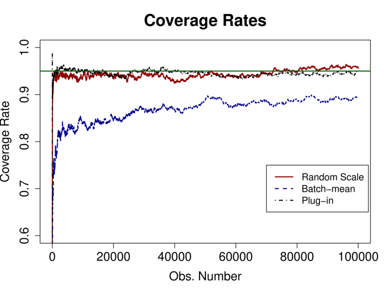
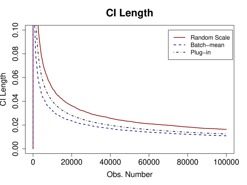
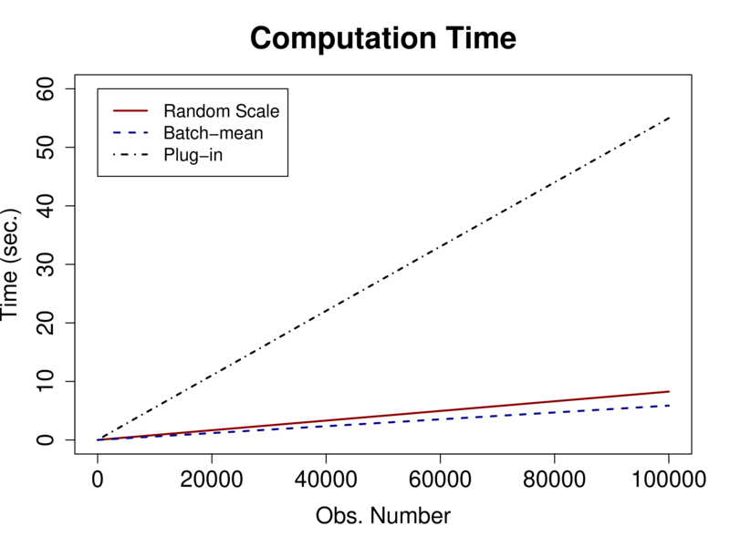
$d=20$

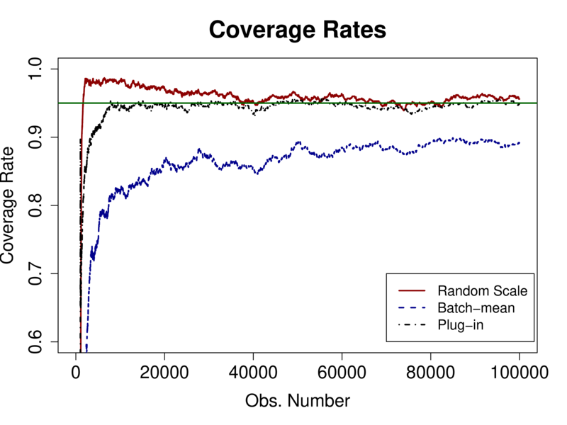
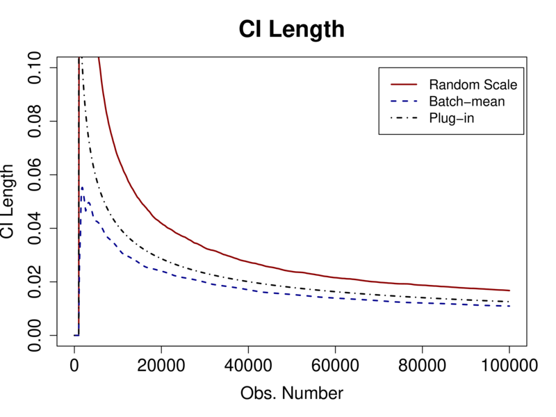
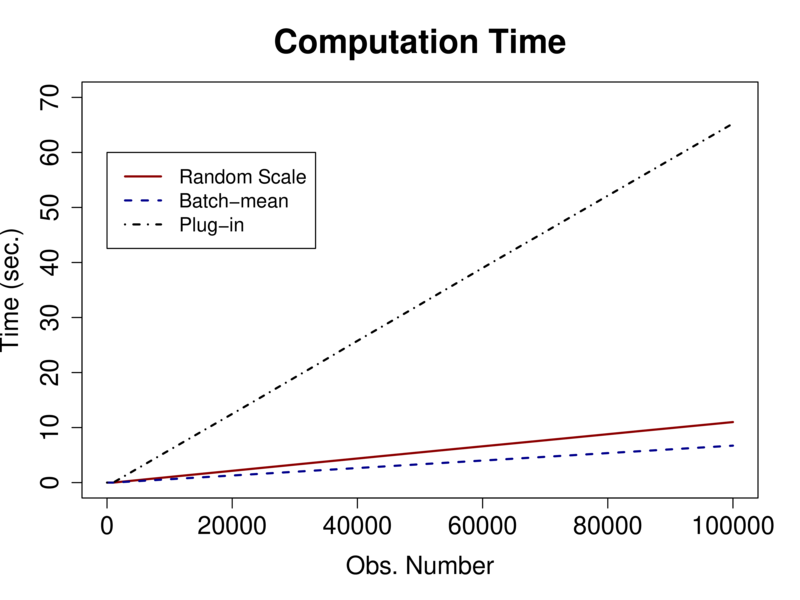
Figure 2: Linear Regression: $d=5$, $\gamma_{0}\in\{0.5,1\}$, $a\in\{0.505,0.667\}$ for $\gamma_{t}=\gamma_{0}t^{-a}$

$\gamma_{0}=0.5,a=0.505$	$\gamma_{0}=0.5,a=0.667$
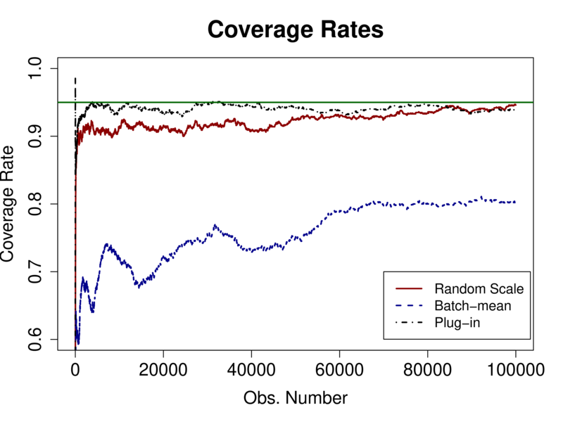
$\gamma_{0}=1,a=0.505$	$\gamma_{0}=1,a=0.667$

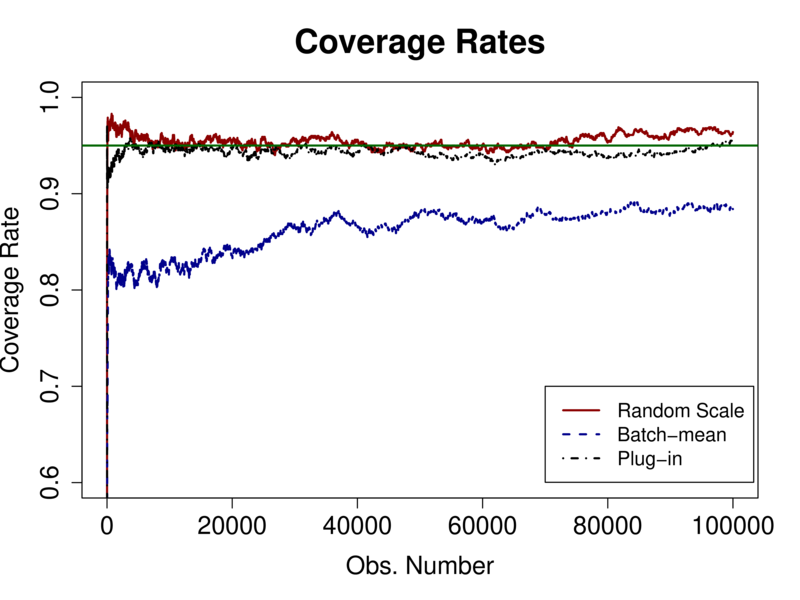
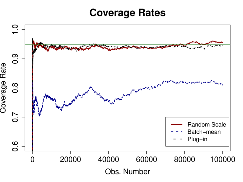
Figures 1–2 summarize the simulation results. The complete set of simulation results are reported in the Appendix. In Figure 1, we adopt the same learning rate parameters as in Zhu et al. (2021): $\gamma_{0}=0.5$ and $a=0.505$. Overall, the performance of the random scaling method is satisfactory. First, the random scaling and plug-in methods show better coverage rates. The coverage rate of the batch-mean method deviates more than 5% from the nominal rate even at $n=100000$. Second, the batch-mean method shows the smallest average length of the confidence interval followed by the plug-in and the random scaling methods. Third, the plug-in method requires substantially more time for computation than the other two methods. The random scaling method takes slightly more computation time than the batch-mean method. Finally, we check the robustness of the performance by changing the learning rates in Figure 2, focusing on the case of $d=5$. Both the random scaling method and the plug-in method are robust to the changes in the learning rates in terms of the coverage rate. However, the batch-mean method converges slowly when $a=0.667$ and it deviates from the nominal rates about 15% even at $n=100000$.

Logistic Regression

We next turn our attention to the following logistic regression model:

$$y_{t}=1(x_{t}^{\prime}\beta^{*}-\varepsilon_{t}\geq 0)~{}~{}\mbox{for}~{}~{}t=1,\ldots,n,$$

where $\varepsilon_{t}$ follows the standard logistic distribution and $1(\cdot)$ is the indicator function. We consider a large dimension of $x_{t}$ ($d=200$) as well as $d=5,20$. All other settings are the same as the linear model.

Table 2: Logistic Regression, $n=10^{5}$, $\gamma_{0}=0.5$, $a=0.505$ for $\gamma_{t}=\gamma_{0}t^{-a}$

	$d=5$	$d=20$	$d=200$
Random Scale
Coverage	0.930	0.929	0.919
Length	0.036	0.043	0.066
Time (sec.)	8.4	11.4	170.3
Batch-mean
Coverage	0.824	0.772	0.644
Length	0.022	0.024	0.027
Time (sec.)	6.0	7.0	10.7
Plug-in
Coverage	0.953	0.946	0.944
Length	0.029	0.035	0.053
Time (sec.)	55.2	66.8	955.0

Overall, the simulation results are similar to those in linear regression. Table 2 summarizes the simulation results of a single design. The coverage rates of Random Scale and Plug-in are satisfactory while that of Batch-mean is 30% lower when $d=200$. Random Scale requires more computation time than Batch-mean but is still much faster than Plug-in. The computation time of Random Scale can be substantially reduced when we are interested in the inference of a single parameter. In such a case, we need to update only a single element of $\hat{V}$ rather than the whole $d\times d$ matrix. In Table 3, we show that Random Scale can be easily scaled up to $d=800$ with only 11.7 seconds computation time when we are interested in the inference of a single parameter. Finally, the results in the appendix reinforce our findings from the linear regression design that the performance of Random-scale is less sensitive to the choice of tuning parameters than Batch-mean.

Table 3: Logistic Regression: Random Scale Updating a Single Element of $\hat{V}$, $n=10^{5}$, $\gamma_{0}=0.5$, $a=0.505$ for $\gamma_{t}=\gamma_{0}t^{-a}$

	$d=5$	$d=20$	$d=200$	$d=500$	$d=800$
Coverage	0.930	0.929	0.919	0.927	0.931
Length	0.037	0.043	0.066	0.133	0.196
Time (sec.)	5.0	5.3	6.7	9.7	11.7

Appendix: Additional Experiment Results

In this section we provide the complete set of simulation results. The R codes to replicate the results are also included in this supplemental package.

Linear Regression: Recall that we the linear regression model is generated from

$$y_{t}=x_{t}^{\prime}\beta^{*}+\varepsilon_{t}~{}~{}\mbox{for}~{}~{}t=1,\ldots,n,$$

where $x_{t}$ is a $d$-dimensional covariates generated from the multivariate normal distribution $\mathcal{N}(0,I_{d})$, $\varepsilon_{t}$ is from $N(0,1)$, and $\beta^{*}$ is equi-spaced on the interval $[0,1]$. The dimension of $x$ is set to $d=5,20$. We consider different combination of the learning rate $\gamma_{t}=\gamma_{0}t^{-a}$ with $1/2<a<1$, where $\gamma_{0}=0.5,1$ and $a=0.505,0.667$. The sample size set to be $n=10^{5}$. The initial value $\beta_{0}$ is set to be zero. In case of $d=20$, we burn in around 1% of observations and start to estimate $\bar{\beta}_{t}$ from $t=1000$. Finally, the simulation results are based on $1000$ replications.

Figure 3 shows the coverage rates and the lengths of the confidence interval for all five coefficients when $d=5$. As discussed in the main text, we observe similar behavior for different coefficients over different learning rates.

Figures 4–5 show the complete paths of coverage rates, confidence interval lengths, and the computation times for each design with different learning rates. Tables 4–5 report the same statistics at $n=25000,50000,75000,$ and $100000$. Overall, the results are in line with our discussion in the main text. The proposed random scaling method and the plug-in method fit the size well while the batch-mean method show less precise coverage rates. The computation time of the plug-in method is at least five times slower than the other two methods. Because the batch size depends on the learning rate parameter $a$, the batch-mean results are sensitive to different learning rates.

Figure 3: Comparison over Different Coefficients: $d=5$

$\gamma_{0}=0.5,a=0.505$

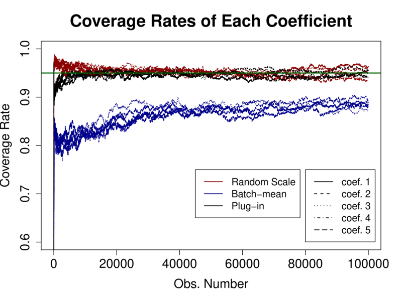
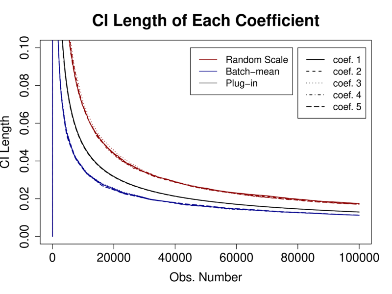
$\gamma_{0}=0.5,a=0.667$

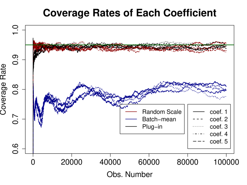
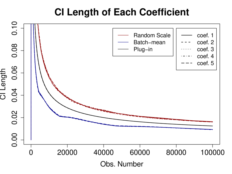
$\gamma_{0}=1,a=0.505$

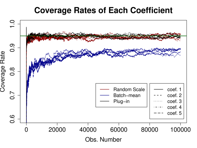
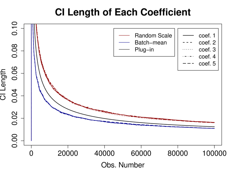
$\gamma_{0}=1,a=0.667$

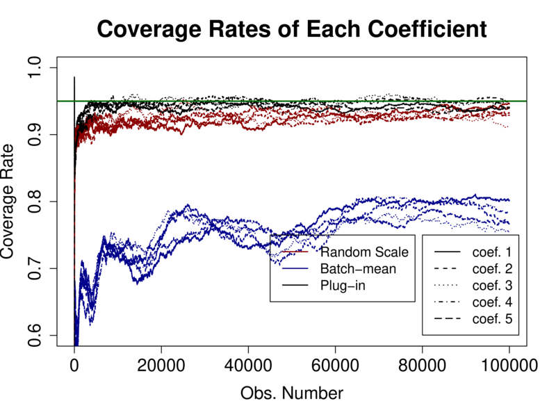
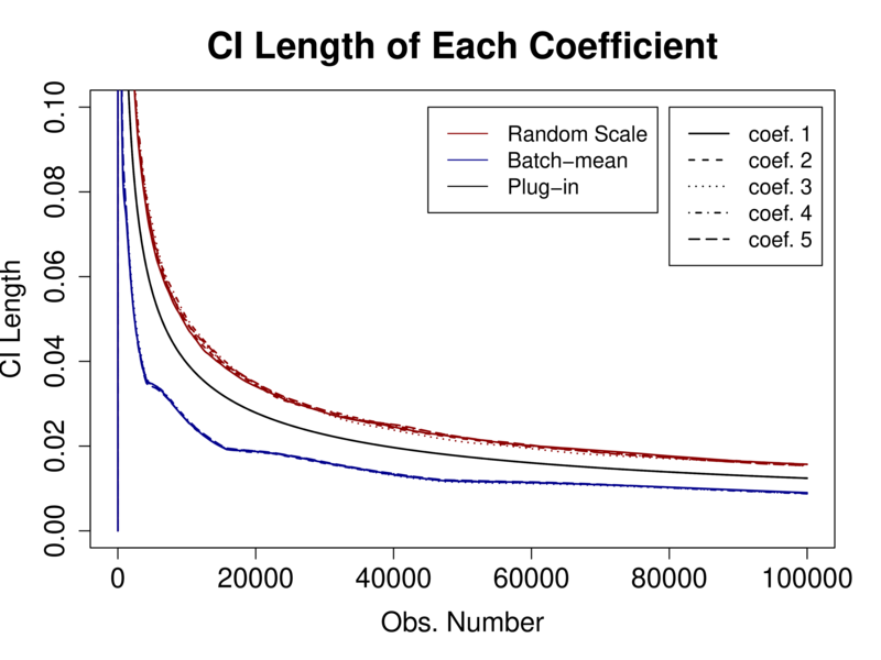
Figure 4: Linear Model: $d=5$, $\gamma_{0}\in\{0.5,1\}$, $a\in\{0.505,0.667\}$ for $\gamma_{t}=\gamma_{0}t^{-a}$

$\gamma_{0}=0.5,a=0.505$

$\gamma_{0}=0.5,a=0.667$

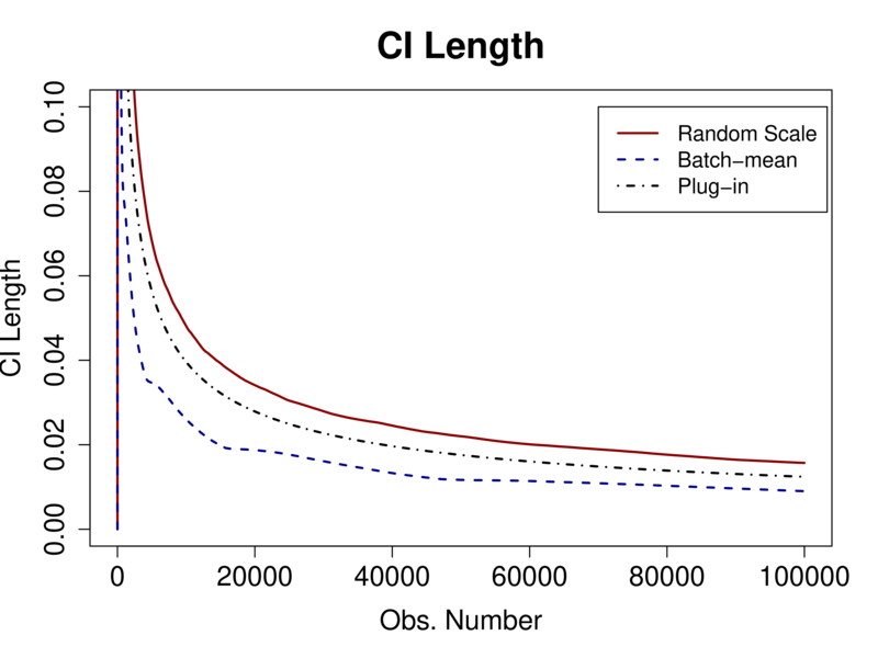
$\gamma_{0}=1,a=0.505$

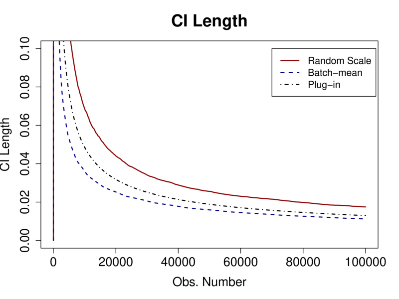
$\gamma_{0}=1,a=0.667$

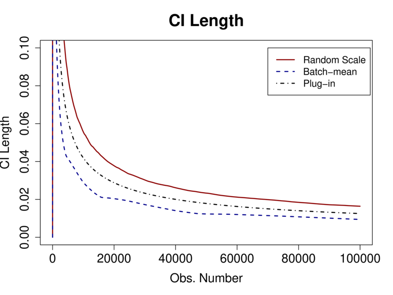
Figure 5: Linear Model: $d=20$, $\gamma_{0}\in\{0.5,1\}$, $a\in\{0.505,0.667\}$ for $\gamma_{t}=\gamma_{0}t^{-a}$

$\gamma_{0}=0.5,a=0.505$

$\gamma_{0}=0.5,a=0.667$

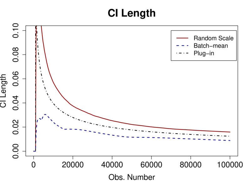
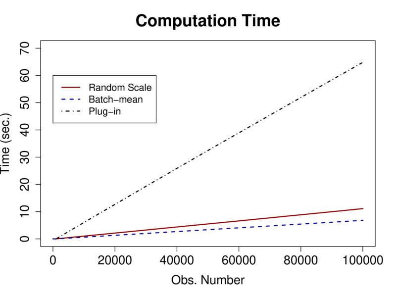
$\gamma_{0}=1,a=0.505$

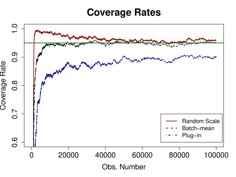
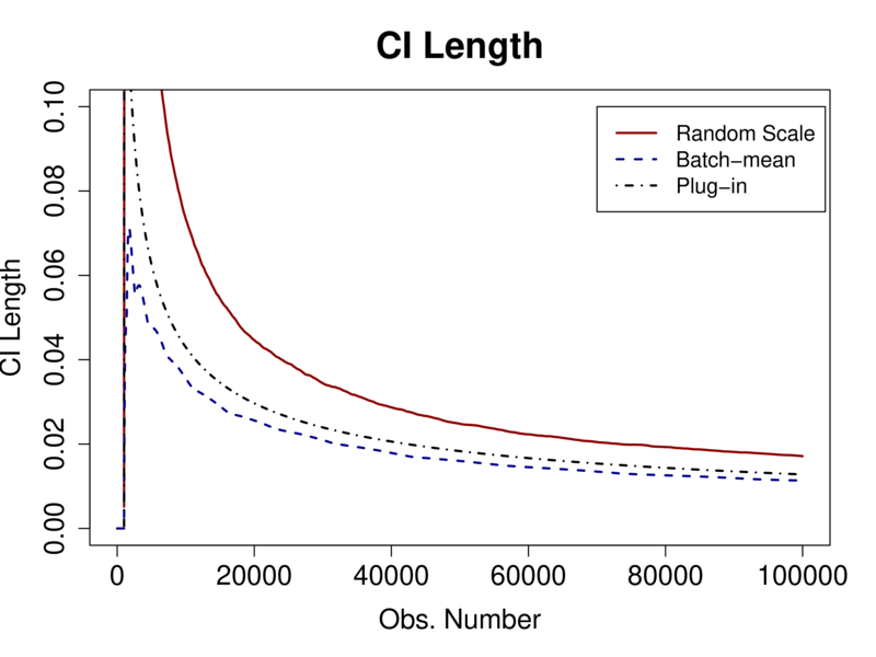
$\gamma_{0}=1,a=0.667$

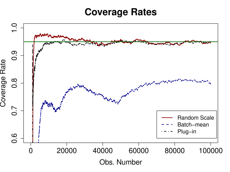
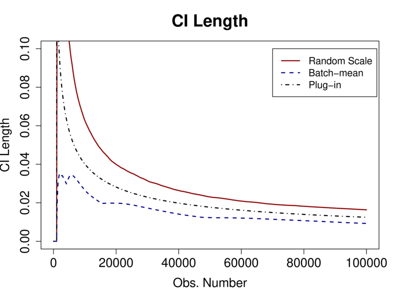
Table 4: Linear Model: $d=5$, $\gamma_{0}\in\{0.5,1\}$, $a\in\{0.505,0.667\}$ for $\gamma_{t}=\gamma_{0}t^{-a}$

		$n=25000$	$n=50000$	$n=75000$	$n=100000$
$\gamma_{0}=0.5,a=0.505$
Coverage	Random Scale	0.941 (0.0075)	0.942 (0.0074)	0.950 (0.0069)	0.957 (0.0064)
	Batch-mean	0.859 (0.0110)	0.888 (0.0100)	0.883 (0.0102)	0.893 (0.0098)
	Plug-in	0.947 (0.0071)	0.947 (0.0071)	0.947 (0.0071)	0.948 (0.0070)
Length	Random Scale	0.032	0.023	0.019	0.016
	Batch-mean	0.021	0.015	0.013	0.011
	Plug-in	0.025	0.018	0.014	0.012
Time (sec.)	Random Scale	2.1	4.1	6.2	8.3
	Batch-mean	1.5	2.9	4.4	5.9
	Plug-in	13.8	27.6	41.3	55.0
$\gamma_{0}=0.5,a=0.667$
Coverage	Random Scale	0.905 (0.0093)	0.924 (0.0084)	0.933 (0.0079)	0.946 (0.0071)
	Batch-mean	0.741 (0.0139)	0.752 (0.0137)	0.793 (0.0128)	0.802 (0.0126)
	Plug-in	0.934 (0.0079)	0.942 (0.0074)	0.945 (0.0072)	0.940 (0.0075)
Length	Random Scale	0.030	0.022	0.018	0.016
	Batch-mean	0.018	0.012	0.011	0.009
	Plug-in	0.025	0.018	0.014	0.012
Time (sec.)	Random Scale	2.1	4.1	6.1	8.2
	Batch-mean	1.5	2.9	4.4	5.8
	Plug-in	13.6	27.1	40.6	54.1
$\gamma_{0}=1,a=0.505$
Coverage	Random Scale	0.957 (0.0064)	0.950 (0.0069)	0.958 (0.0063)	0.964 (0.0059)
	Batch-mean	0.849 (0.0113)	0.880 (0.0103)	0.875 (0.0105)	0.884 (0.0101)
	Plug-in	0.947 (0.0071)	0.941 (0.0075)	0.943 (0.0073)	0.956 (0.0065)
Length	Random Scale	0.038	0.026	0.021	0.018
	Batch-mean	0.022	0.016	0.013	0.011
	Plug-in	0.028	0.019	0.015	0.013
Time (sec.)	Random Scale	2.1	4.2	6.3	8.4
	Batch-mean	1.5	3.0	4.5	6.0
	Plug-in	13.9	27.7	41.6	55.4
$\gamma_{0}=1,a=0.667$
Coverage	Random Scale	0.933 (0.0079)	0.936 (0.0077)	0.946 (0.0071)	0.956 (0.0065)
	Batch-mean	0.773 (0.0132)	0.774 (0.0132)	0.820 (0.0121)	0.810 (0.0124)
	Plug-in	0.942 (0.0074)	0.942 (0.0074)	0.943 (0.0073)	0.946 (0.0071)
Length	Random Scale	0.033	0.023	0.019	0.016
	Batch-mean	0.019	0.012	0.011	0.009
	Plug-in	0.026	0.018	0.014	0.013
Time (sec.)	Random Scale	2.1	4.1	6.1	8.2
	Batch-mean	1.5	2.9	4.4	5.8
	Plug-in	13.5	26.9	40.4	53.9

Table 5: Linear Model: $d=20$, $\gamma_{0}\in\{0.5,1\}$, $a\in\{0.505,0.667\}$ for $\gamma_{t}=\gamma_{0}t^{-a}$

		$n=25000$	$n=50000$	$n=75000$	$n=100000$
$\gamma_{0}=0.5,a=0.505$
Coverage	Random Scale	0.963 (0.0060)	0.960 (0.0062)	0.949 (0.0070)	0.956 (0.0065)
	Batch-mean	0.860 (0.0110)	0.890 (0.0099)	0.878 (0.0103)	0.890 (0.0099)
	Plug-in	0.938 (0.0076)	0.954 (0.0066)	0.937 (0.0077)	0.949 (0.0070)
Length	Random Scale	0.037	0.024	0.019	0.017
	Batch-mean	0.022	0.015	0.012	0.011
	Plug-in	0.026	0.018	0.015	0.013
Time (sec.)	Random Scale	2.7	5.5	8.2	11.0
	Batch-mean	1.6	3.3	5.0	6.7
	Plug-in	15.8	32.4	48.9	65.2
$\gamma_{0}=0.5,a=0.667$
Coverage	Random Scale	0.941 (0.0075)	0.935 (0.0078)	0.928 (0.0082)	0.933 (0.0079)
	Batch-mean	0.751 (0.0137)	0.724 (0.0141)	0.778 (0.0131)	0.777 (0.0132)
	Plug-in	0.938 (0.0076)	0.946 (0.0071)	0.944 (0.0073)	0.948 (0.0070)
Length	Random Scale	0.033	0.022	0.018	0.016
	Batch-mean	0.018	0.012	0.010	0.009
	Plug-in	0.025	0.018	0.014	0.012
Time (sec.)	Random Scale	2.7	5.5	8.3	11.1
	Batch-mean	1.7	3.4	5.1	6.8
	Plug-in	16.0	32.4	48.7	64.8
$\gamma_{0}=1,a=0.505$
Coverage	Random Scale	0.968 (0.0056)	0.961 (0.0061)	0.952 (0.0068)	0.960 (0.0062)
	Batch-mean	0.857 (0.0111)	0.899 (0.0095)	0.876 (0.0104)	0.897 (0.0096)
	Plug-in	0.942 (0.0074)	0.952 (0.0068)	0.938 (0.0076)	0.954 (0.0066)
Length	Random Scale	14.426	7.230	4.826	3.622
	Batch-mean	3.389	1.457	0.938	0.661
	Plug-in	16.776	8.359	5.549	4.151
Time (sec.)	Random Scale	2.7	5.4	8.1	10.9
	Batch-mean	1.6	3.3	5.0	6.6
	Plug-in	15.5	31.7	47.8	63.9
$\gamma_{0}=1,a=0.667$
Coverage	Random Scale	0.955 (0.0066)	0.959 (0.0063)	0.948 (0.0070)	0.946 (0.0071)
	Batch-mean	0.789 (0.0129)	0.739 (0.0139)	0.806 (0.0125)	0.797 (0.0127)
	Plug-in	0.939 (0.0076)	0.953 (0.0067)	0.943 (0.0073)	0.949 (0.0070)
Length	Random Scale	0.035	0.023	0.019	0.016
	Batch-mean	0.019	0.012	0.011	0.009
	Plug-in	0.025	0.018	0.014	0.012
Time (sec.)	Random Scale	2.6	5.4	8.1	10.8
	Batch-mean	1.6	3.3	5.0	6.6
	Plug-in	15.5	31.6	47.8	64.0

Logistic Regression: Recall that we the logistic regression model is generated from

$$y_{t}=1(x_{t}^{\prime}\beta^{*}-\varepsilon_{t}\geq 0)~{}~{}\mbox{for}~{}~{}t=1,\ldots,n,$$

where $\varepsilon_{t}$ follows the standard logistic distribution and $1(\cdot)$ is the indicator function. We consider $d=5,20,200$. All other settings are the same as the linear model.

Figures 6–8 show the complete paths of coverage rates, confidence interval lengths, and the computation times for each design with different learning rates. Tables 6–8 report the same statistics at $n=25000,50000,75000,$ and $100000$. Overall, the results are similar to those of the linear regression model. The proposed random scaling method and the plug-in method fit the size well while the batch-mean method show less precise coverage rates. The computation time of the plug-in method is at least five times slower than the other two methods. Because the batch size depends on the learning rate parameter $a$, the batch-mean results are sensitive to different learning rates. For the large model $d=200$, the plug-in method does not perform well in terms of the coverage rate when $a=0.667$.

Figure 6: Logistic Model: $d=5$, $\gamma_{0}\in\{0.5,1\}$, $a\in\{0.505,0.667\}$ for $\gamma_{t}=\gamma_{0}t^{-a}$

$\gamma_{0}=0.5,a=0.505$

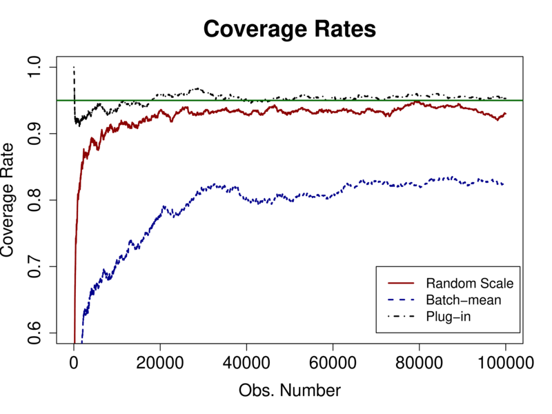
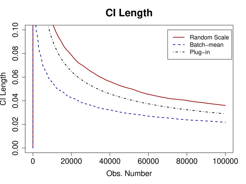
$\gamma_{0}=0.5,a=0.667$

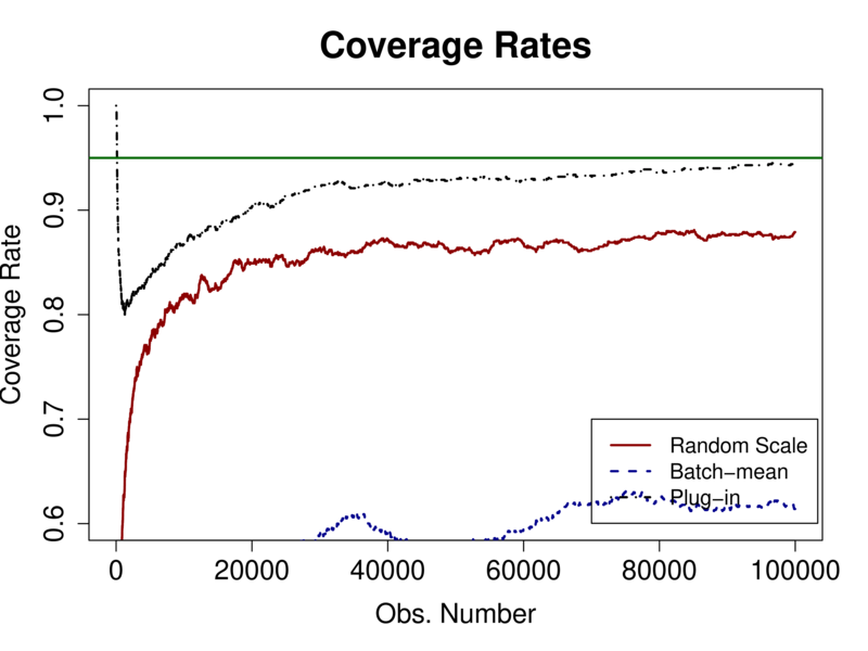
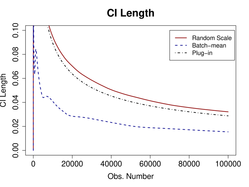
$\gamma_{0}=1,a=0.505$

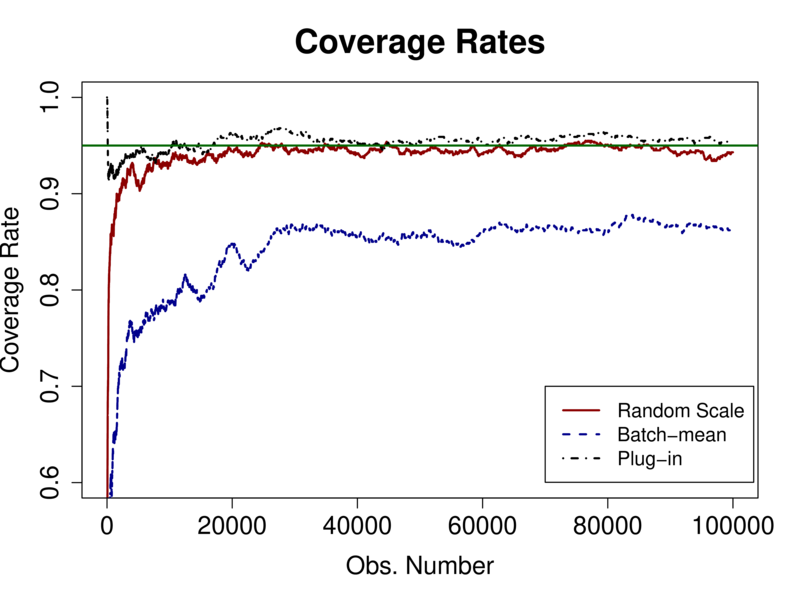
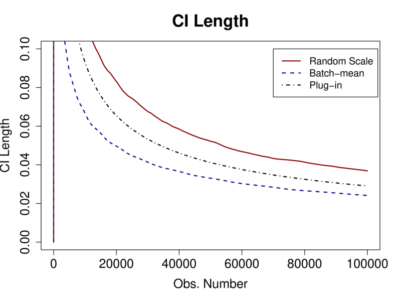
$\gamma_{0}=1,a=0.667$

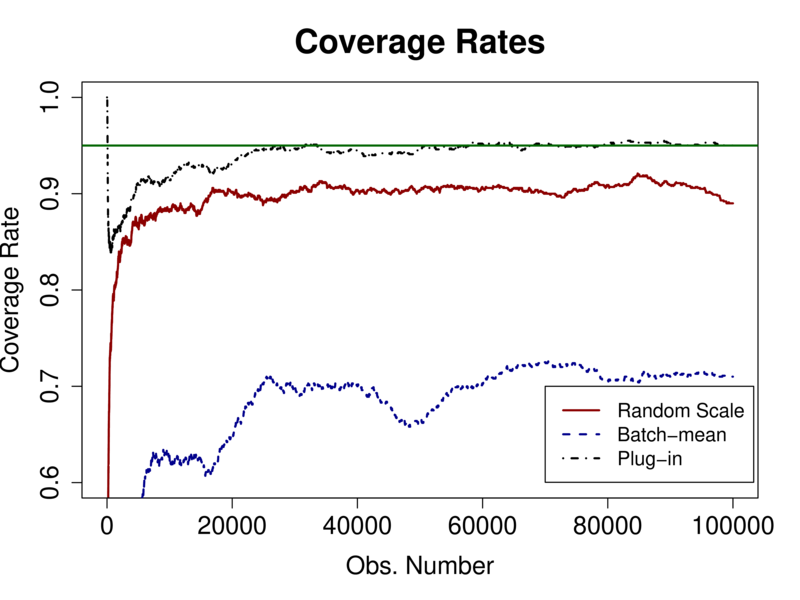
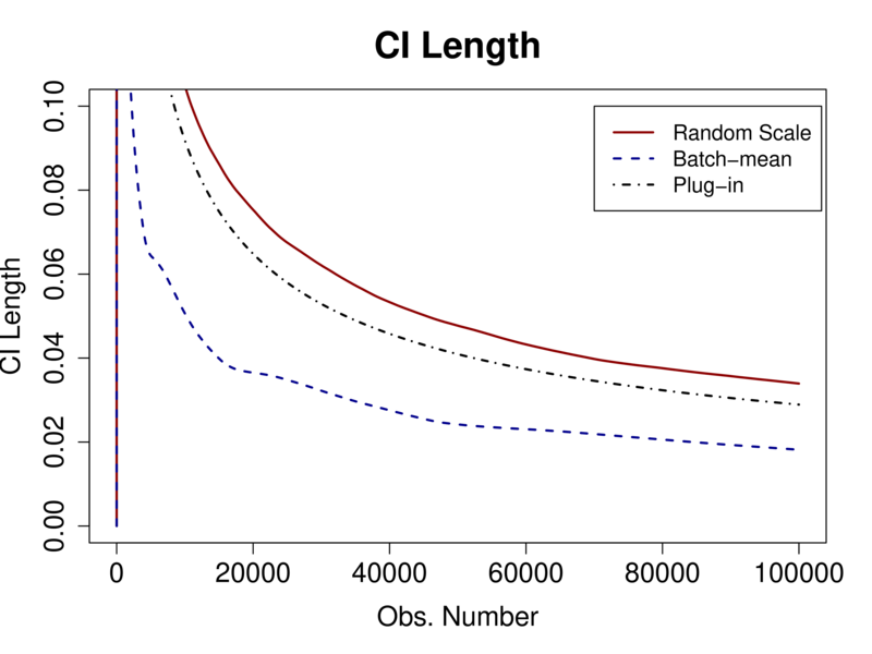
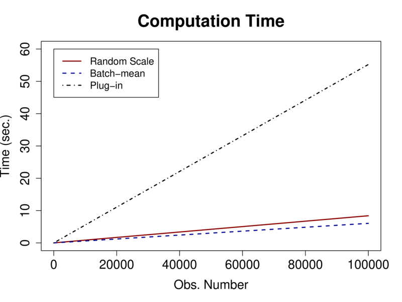
Figure 7: Logistic Model: $d=20$, $\gamma_{0}\in\{0.5,1\}$, $a\in\{0.505,0.667\}$ for $\gamma_{t}=\gamma_{0}t^{-a}$

$\gamma_{0}=0.5,a=0.505$

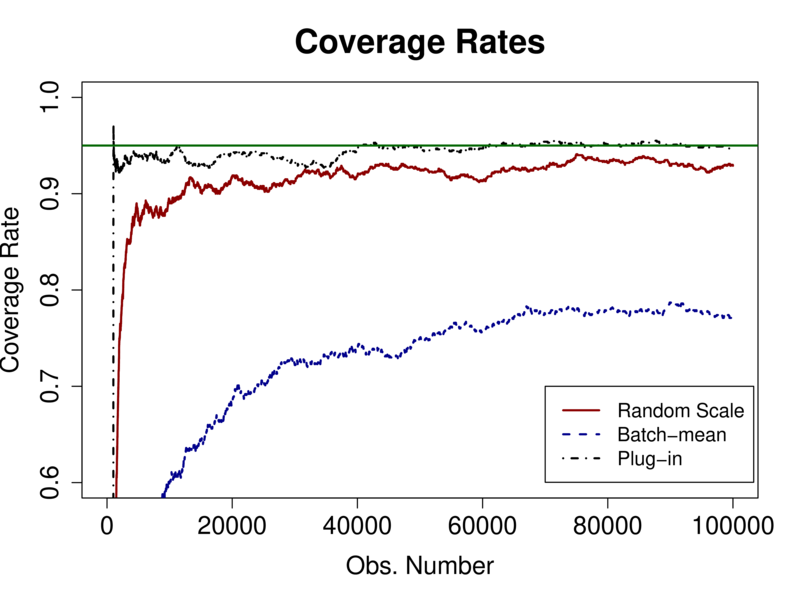
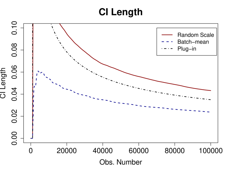
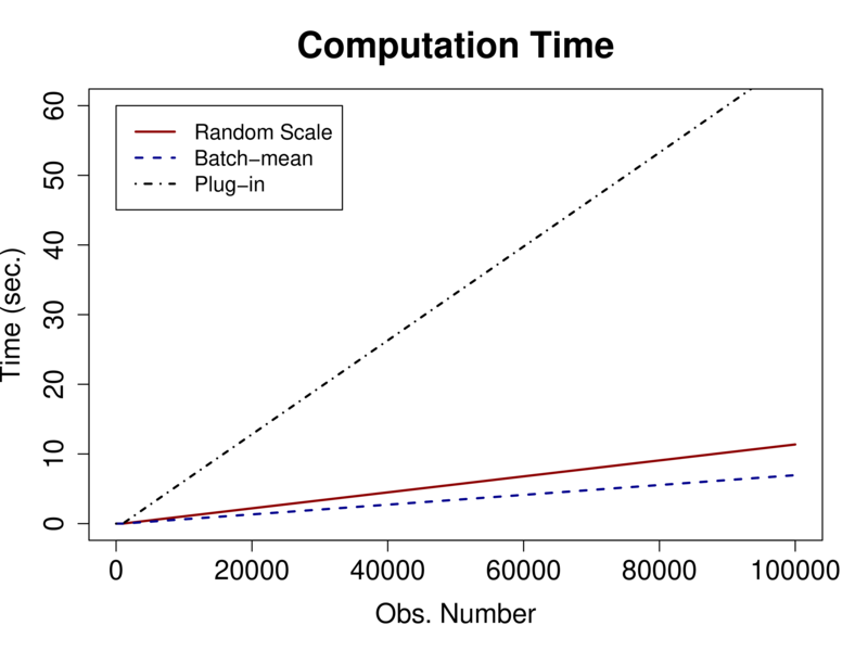
$\gamma_{0}=0.5,a=0.667$

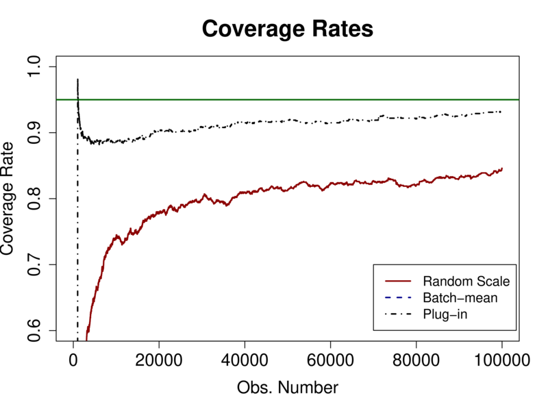
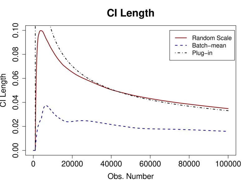
$\gamma_{0}=1,a=0.505$

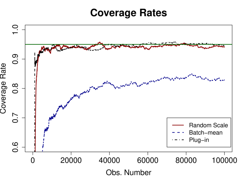
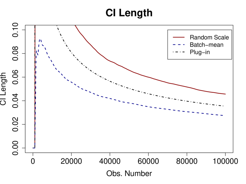
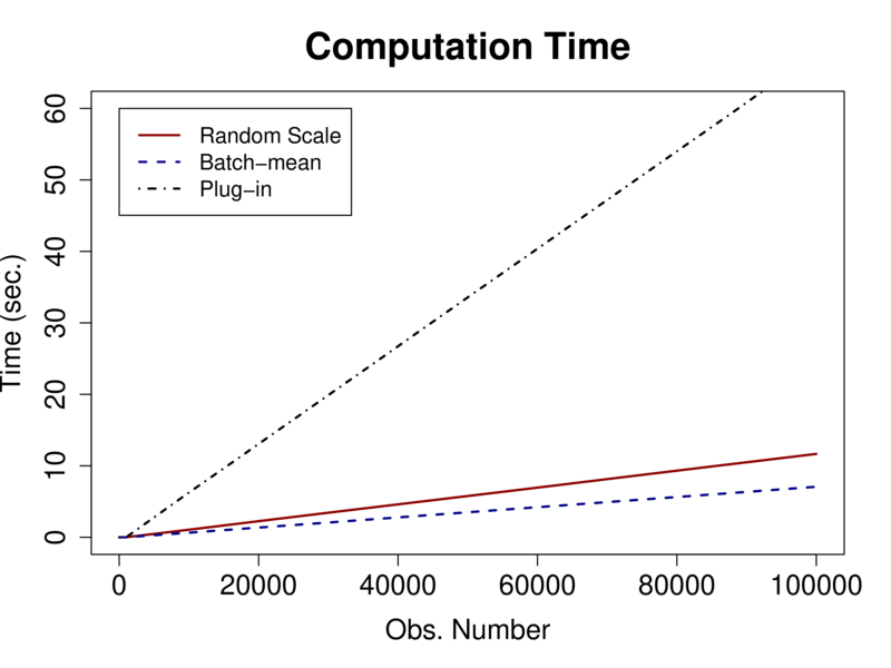
$\gamma_{0}=1,a=0.667$

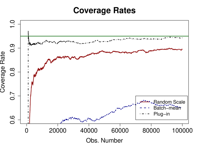
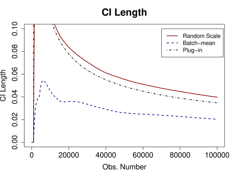
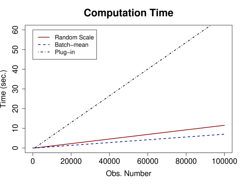
Figure 8: Logistic Model: $d=200$, $\gamma_{0}\in\{0.5,1\}$, $a\in\{0.505,0.667\}$ for $\gamma_{t}=\gamma_{0}t^{-a}$

$\gamma_{0}=0.5,a=0.505$

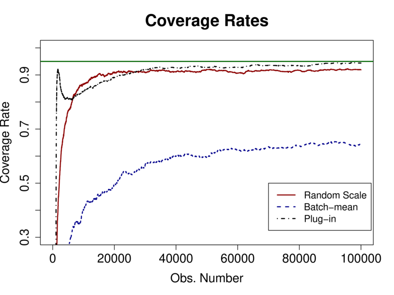
$\gamma_{0}=0.5,a=0.667$

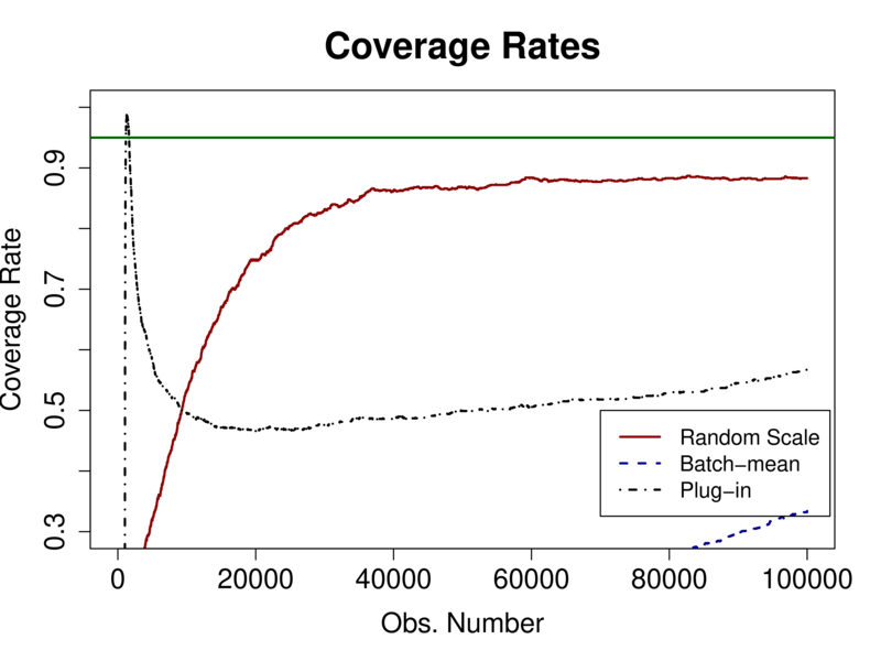
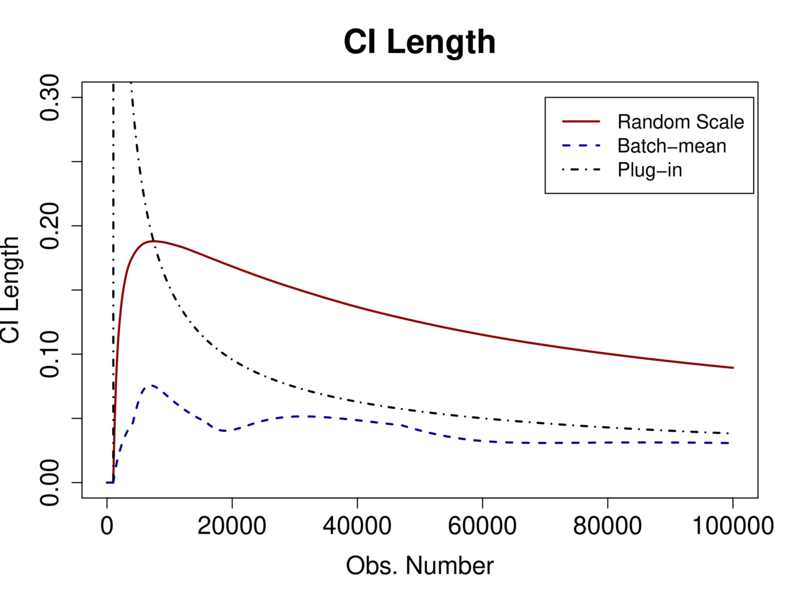
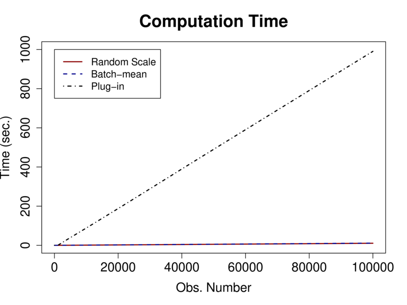
$\gamma_{0}=1,a=0.505$

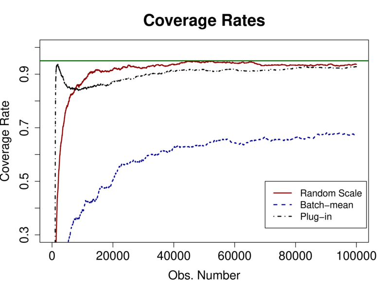
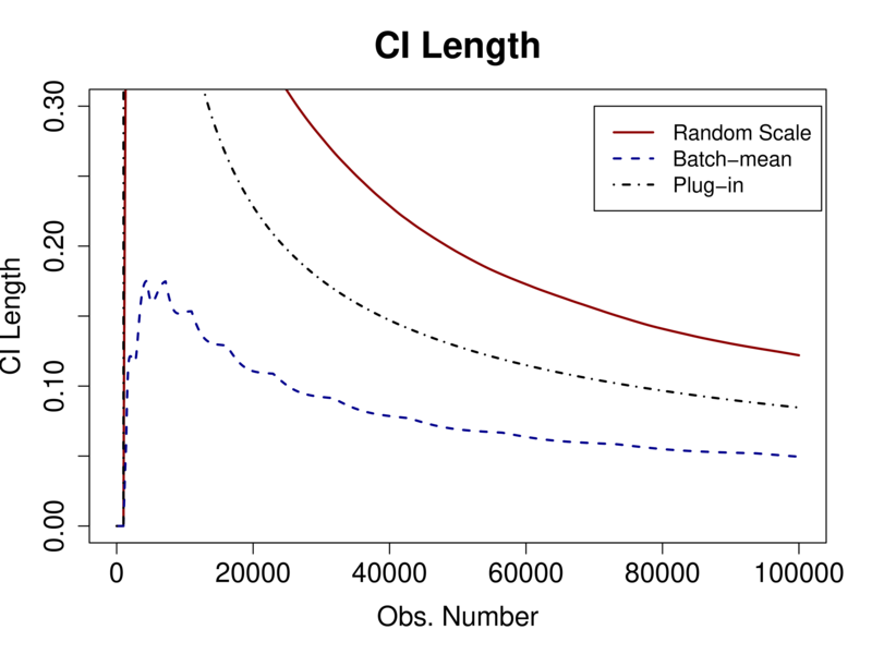
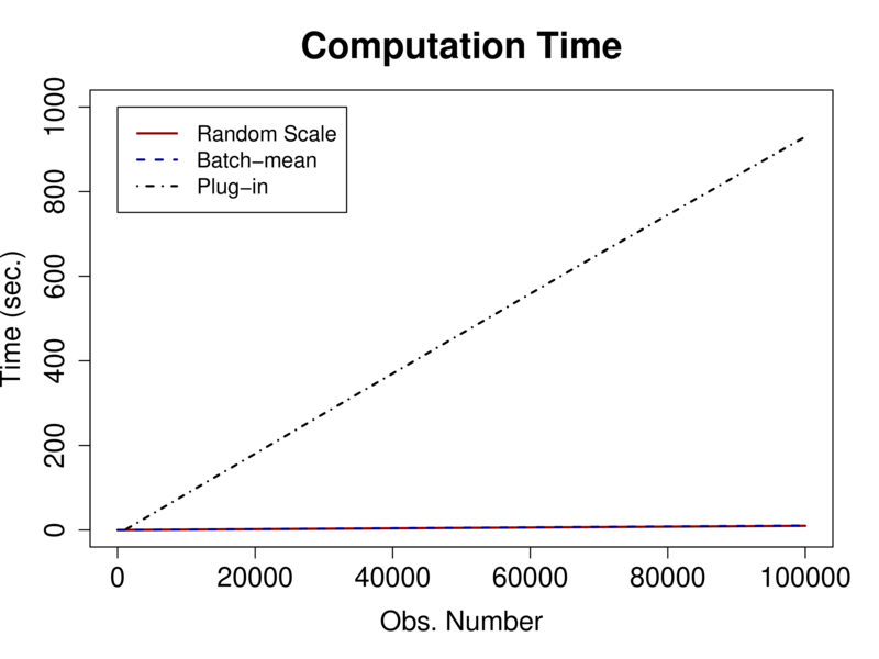
$\gamma_{0}=1,a=0.667$

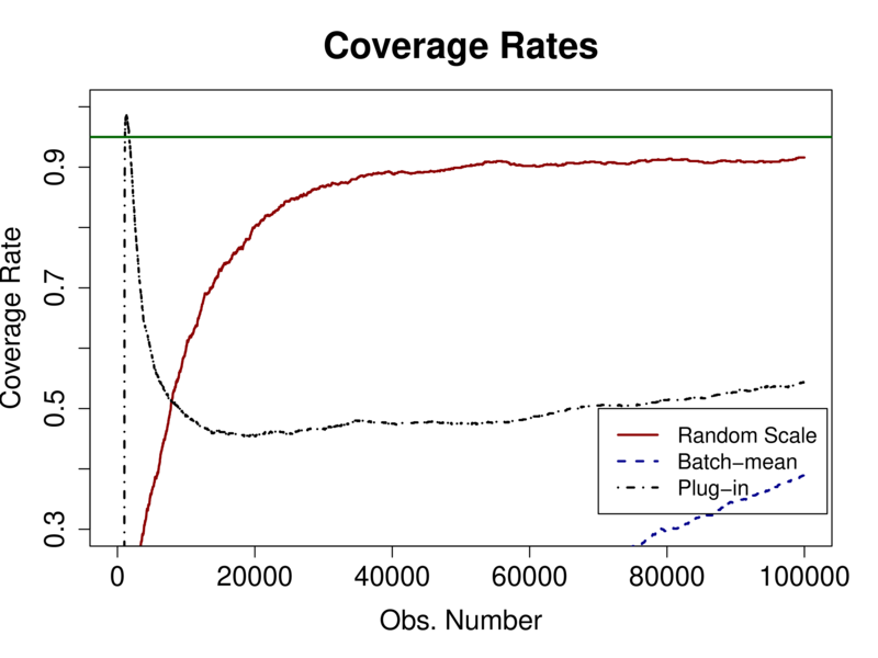
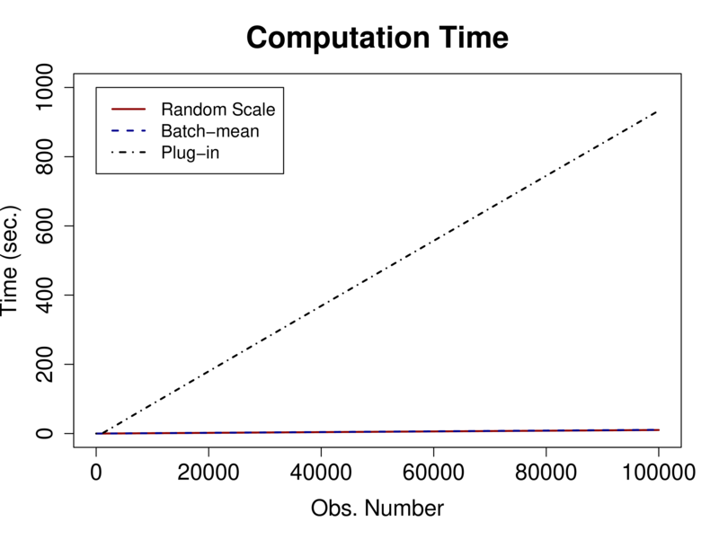
Table 6: Logistic Model: $d=5$, $\gamma_{0}\in\{0.5,1\}$, $a\in\{0.505,0.667\}$ for $\gamma_{t}=\gamma_{0}t^{-a}$

		$n=25000$	$n=50000$	$n=75000$	$n=100000$
$\gamma_{0}=0.5,a=0.505$
Coverage	Random Scale	0.937 (0.0077)	0.930 (0.0081)	0.939 (0.0076)	0.930 (0.0081)
	Batch-mean	0.786 (0.0130)	0.799 (0.0127)	0.821 (0.0121)	0.824 (0.0120)
	Plug-in	0.960 (0.0062)	0.951 (0.0068)	0.955 (0.0066)	0.953 (0.0067)
Length	Random Scale	0.071	0.050	0.041	0.036
	Batch-mean	0.039	0.029	0.025	0.022
	Plug-in	0.058	0.041	0.033	0.029
Time (sec.)	Random Scale	2.1	4.2	6.3	8.4
	Batch-mean	1.5	3.0	4.5	6.0
	Plug-in	13.8	27.6	41.4	55.2
$\gamma_{0}=0.5,a=0.667$
Coverage	Random Scale	0.848 (0.0114)	0.862 (0.0109)	0.871 (0.0106)	0.879 (0.0103)
	Batch-mean	0.566 (0.0157)	0.578 (0.0156)	0.630 (0.0153)	0.614 (0.0154)
	Plug-in	0.914 (0.0089)	0.930 (0.0081)	0.936 (0.0077)	0.945 (0.0072)
Length	Random Scale	0.063	0.045	0.037	0.032
	Batch-mean	0.028	0.020	0.018	0.015
	Plug-in	0.057	0.041	0.033	0.029
Time (sec.)	Random Scale	2.1	4.3	6.4	8.5
	Batch-mean	1.5	3.1	4.6	6.1
	Plug-in	14.0	28.0	42.0	56.0
$\gamma_{0}=1,a=0.505$
Coverage	Random Scale	0.952 (0.0068)	0.942 (0.0074)	0.952 (0.0068)	0.943 (0.0073)
	Batch-mean	0.841 (0.0116)	0.855 (0.0111)	0.862 (0.0109)	0.863 (0.0109)
	Plug-in	0.959 (0.0063)	0.953 (0.0067)	0.959 (0.0063)	0.952 (0.0068)
Length	Random Scale	0.074	0.052	0.042	0.037
	Batch-mean	0.045	0.033	0.027	0.024
	Plug-in	0.058	0.041	0.034	0.029
Time (sec.)	Random Scale	2.1	4.2	6.3	8.4
	Batch-mean	1.5	3.0	4.5	6.1
	Plug-in	13.8	27.6	41.3	55.1
$\gamma_{0}=1,a=0.667$
Coverage	Random Scale	0.892 (0.0098)	0.904 (0.0093)	0.904 (0.0093)	0.890 (0.0099)
	Batch-mean	0.702 (0.0145)	0.662 (0.0150)	0.722 (0.0142)	0.710 (0.0143)
	Plug-in	0.945 (0.0072)	0.946 (0.0071)	0.949 (0.0070)	0.950 (0.0069)
Length	Random Scale	0.068	0.048	0.039	0.034
	Batch-mean	0.035	0.024	0.021	0.018
	Plug-in	0.058	0.041	0.033	0.029
Time (sec.)	Random Scale	2.1	4.2	6.3	8.4
	Batch-mean	1.5	3.0	4.5	6.1
	Plug-in	13.8	27.6	41.4	55.2

Table 7: Logistic Model: $d=20$, $\gamma_{0}\in\{0.5,1\}$, $a\in\{0.505,0.667\}$ for $\gamma_{t}=\gamma_{0}t^{-a}$

		$n=25000$	$n=50000$	$n=75000$	$n=100000$
$\gamma_{0}=0.5,a=0.505$
Coverage	Random Scale	0.908 (0.0091)	0.925 (0.0083)	0.941 (0.0075)	0.929 (0.0081)
	Batch-mean	0.704 (0.0144)	0.750 (0.0137)	0.780 (0.0131)	0.772 (0.0133)
	Plug-in	0.942 (0.0074)	0.947 (0.0071)	0.953 (0.0067)	0.946 (0.0071)
Length	Random Scale	0.086	0.061	0.050	0.043
	Batch-mean	0.041	0.032	0.027	0.024
	Plug-in	0.070	0.050	0.040	0.035
Time (sec.)	Random Scale	2.8	5.6	8.5	11.4
	Batch-mean	1.7	3.4	5.2	7.0
	Plug-in	16.2	33.0	49.9	66.8
$\gamma_{0}=0.5,a=0.667$
Coverage	Random Scale	0.788 (0.0129)	0.813 (0.0123)	0.828 (0.0119)	0.846 (0.0114)
	Batch-mean	0.456 (0.0158)	0.480 (0.0158)	0.527 (0.0158)	0.549 (0.0157)
	Plug-in	0.902 (0.0094)	0.919 (0.0086)	0.922 (0.0085)	0.932 (0.0080)
Length	Random Scale	0.061	0.046	0.039	0.035
	Batch-mean	0.025	0.019	0.017	0.016
	Plug-in	0.063	0.046	0.038	0.033
Time (sec.)	Random Scale	2.8	5.6	8.5	11.3
	Batch-mean	1.7	3.4	5.2	6.9
	Plug-in	16.2	33.1	50.0	66.9
$\gamma_{0}=1,a=0.505$
Coverage	Random Scale	0.939 (0.0076)	0.942 (0.0074)	0.945 (0.0072)	0.941 (0.0075)
	Batch-mean	0.782 (0.0131)	0.812 (0.0124)	0.838 (0.0117)	0.829 (0.0119)
	Plug-in	0.942 (0.0074)	0.947 (0.0071)	0.952 (0.0068)	0.943 (0.0073)
Length	Random Scale	0.097	0.066	0.053	0.046
	Batch-mean	0.050	0.038	0.032	0.027
	Plug-in	0.072	0.050	0.041	0.035
Time (sec.)	Random Scale	2.8	5.8	8.7	11.7
	Batch-mean	1.7	3.5	5.3	7.1
	Plug-in	16.5	33.6	50.6	67.7
$\gamma_{0}=1,a=0.667$
Coverage	Random Scale	0.863 (0.0109)	0.885 (0.0101)	0.891 (0.0099)	0.895 (0.0097)
	Batch-mean	0.604 (0.0155)	0.614 (0.0154)	0.681 (0.0147)	0.653 (0.0151)
	Plug-in	0.924 (0.0084)	0.928 (0.0082)	0.939 (0.0076)	0.944 (0.0073)
Length	Random Scale	0.076	0.055	0.046	0.040
	Batch-mean	0.036	0.026	0.023	0.020
	Plug-in	0.070	0.049	0.040	0.035
Time (sec.)	Random Scale	2.8	5.7	8.6	11.5
	Batch-mean	1.7	3.5	5.2	7.0
	Plug-in	16.3	33.3	50.2	67.2

Table 8: Logistic Model: $d=200$, $\gamma_{0}\in\{0.5,1\}$, $a\in\{0.505,0.667\}$ for $\gamma_{t}=\gamma_{0}t^{-a}$

		$n=25000$	$n=50000$	$n=75000$	$n=100000$
$\gamma_{0}=0.5,a=0.505$
Coverage	Random Scale	0.914 (0.0089)	0.920 (0.0086)	0.912 (0.0090)	0.919 (0.0086)
	Batch-mean	0.534 (0.0158)	0.594 (0.0155)	0.630 (0.0153)	0.644 (0.0151)
	Plug-in	0.904 (0.0093)	0.928 (0.0082)	0.935 (0.0078)	0.944 (0.0073)
Length	Random Scale	0.153	0.100	0.078	0.066
	Batch-mean	0.050	0.036	0.031	0.027
	Plug-in	0.108	0.075	0.061	0.053
Time (sec.)	Random Scale	41.4	84.6	127.6	170.3
	Batch-mean	2.6	5.3	8.0	10.7
	Plug-in	231.4	472.6	714.3	955.0
$\gamma_{0}=0.5,a=0.667$
Coverage	Random Scale	0.804 (0.0126)	0.868 (0.0107)	0.881 (0.0102)	0.883 (0.0102)
	Batch-mean	0.165 (0.0117)	0.216 (0.0130)	0.244 (0.0136)	0.334 (0.0149)
	Plug-in	0.467 (0.0158)	0.499 (0.0158)	0.521 (0.0158)	0.567 (0.0157)
Length	Random Scale	0.159	0.125	0.104	0.089
	Batch-mean	0.048	0.041	0.031	0.031
	Plug-in	0.083	0.055	0.044	0.038
Time (sec.)	Random Scale	2.6	5.2	7.9	10.5
	Batch-mean	2.7	5.5	8.3	11.1
	Plug-in	238.2	490.3	740.6	990.6
$\gamma_{0}=1,a=0.505$
Coverage	Random Scale	0.933 (0.0079)	0.944 (0.0073)	0.934 (0.0079)	0.937 (0.0077)
	Batch-mean	0.566 (0.0157)	0.631 (0.0153)	0.656 (0.0150)	0.674 (0.0148)
	Plug-in	0.884 (0.0101)	0.916 (0.0088)	0.917 (0.0087)	0.928 (0.0082)
Length	Random Scale	0.311	0.196	0.148	0.122
	Batch-mean	0.100	0.069	0.058	0.050
	Plug-in	0.197	0.128	0.101	0.085
Time (sec.)	Random Scale	2.4	4.9	7.4	9.9
	Batch-mean	2.5	5.2	7.8	10.5
	Plug-in	227.9	464.5	698.8	929.6
$\gamma_{0}=1,a=0.667$
Coverage	Random Scale	0.844 (0.0115)	0.899 (0.0095)	0.908 (0.0091)	0.916 (0.0088)
	Batch-mean	0.166 (0.0118)	0.257 (0.0138)	0.272 (0.0141)	0.389 (0.0154)
	Plug-in	0.458 (0.0158)	0.475 (0.0158)	0.505 (0.0158)	0.543 (0.0158)
Length	Random Scale	0.329	0.250	0.203	0.173
	Batch-mean	0.099	0.083	0.061	0.059
	Plug-in	0.148	0.094	0.074	0.062
Time (sec.)	Random Scale	2.5	5.0	7.6	10.1
	Batch-mean	2.6	5.3	8.0	10.7
	Plug-in	227.1	462.9	698.0	933.0

References

- Abadir and Paruolo (1997) Abadir, K. M. and P. Paruolo (1997). Two mixed normal densities from cointegration analysis. Econometrica 65(3), 671–680.
- Anastasiou et al. (2019) Anastasiou, A., K. Balasubramanian, and M. A. Erdogdu (2019). Normal approximation for stochastic gradient descent via non-asymptotic rates of martingale CLT. In A. Beygelzimer and D. Hsu (Eds.), Proceedings of the Thirty-Second Conference on Learning Theory, Volume 99 of Proceedings of Machine Learning Research, pp. 115–137.
- Bach and Moulines (2013) Bach, F. and E. Moulines (2013). Non-strongly-convex smooth stochastic approximation with convergence rate O (1/n). In Advances in Neural Information Processing Systems (NIPS).
- Chen et al. (2020) Chen, X., J. D. Lee, X. T. Tong, and Y. Zhang (2020). Statistical inference for model parameters in stochastic gradient descent. Annals of Statistics 48(1), 251–273.
- Duchi et al. (2011) Duchi, J., E. Hazan, and Y. Singer (2011). Adaptive subgradient methods for online learning and stochastic optimization. Journal of Machine Learning Research 12(7), 2121–2159.
- Fang et al. (2018) Fang, Y., J. Xu, and L. Yang (2018). Online bootstrap confidence intervals for the stochastic gradient descent estimator. Journal of Machine Learning Research 19(1), 1–21.
- Godichon-Baggioni (2017) Godichon-Baggioni, A. (2017). A central limit theorem for averaged stochastic gradient algorithms in hilbert spaces and online estimation of the asymptotic variance. application to the geometric median and quantiles. arXiv:1702.00931v1 [math.ST], available at https://arxiv.org/pdf/1702.00931v1.pdf.
- Gupta and Seo (2021) Gupta, A. and M. H. Seo (2021). Robust inference on infinite and growing dimensional regression. arXiv:1911.08637 [econ.EM], available at https://arxiv.org/abs/1911.08637v2.
- Hall and Heyde (1980) Hall, P. and C. C. Heyde (1980). Martingale Limit Theory and Its Application. Academic Press, Boston,.
- Hazan and Kale (2014) Hazan, E. and S. Kale (2014). Beyond the regret minimization barrier: optimal algorithms for stochastic strongly-convex optimization. Journal of Machine Learning Research 15(1), 2489–2512.
- Hoffman et al. (2010) Hoffman, M. D., D. M. Blei, and F. Bach (2010). Online learning for latent dirichlet allocation. In Proceedings of the 23rd International Conference on Neural Information Processing Systems, NIPS’10, pp. 856–864.
- Kiefer et al. (2000) Kiefer, N. M., T. J. Vogelsang, and H. Bunzel (2000). Simple robust testing of regression hypotheses. Econometrica 68(3), 695–714.
- Kim and Sun (2011) Kim, M. S. and Y. Sun (2011). Spatial heteroskedasticity and autocorrelation consistent estimation of covariance matrix. Journal of Econometrics 160(2), 349–371.
- Kingma and Ba (2015) Kingma, D. P. and J. Ba (2015). Adam: A method for stochastic optimization. In Y. Bengio and Y. LeCun (Eds.), 3rd International Conference on Learning Representations, ICLR 2015, San Diego, CA, USA, May 7-9, 2015, Conference Track Proceedings.
- Kushner and Yang (1993) Kushner, H. J. and J. Yang (1993). Stochastic approximation with averaging of the iterates: Optimal asymptotic rate of convergence for general processes. SIAM Journal on Control and Optimization 31(4), 1045–1062.
- Lazarus et al. (2018) Lazarus, E., D. J. Lewis, J. H. Stock, and M. W. Watson (2018). Har inference: Recommendations for practice. Journal of Business & Economic Statistics 36(4), 541–559.
- Liang and Su (2019) Liang, T. and W. J. Su (2019). Statistical inference for the population landscape via moment-adjusted stochastic gradients. Journal of the Royal Statistical Society: Series B (Statistical Methodology) 81(2), 431–456.
- Mairal et al. (2010) Mairal, J., F. Bach, J. Ponce, and G. Sapiro (2010). Online learning for matrix factorization and sparse coding. Journal of Machine Learning Research 11(1), 19–60.
- Mou et al. (2020) Mou, W., C. J. Li, M. J. Wainwright, P. L. Bartlett, and M. I. Jordan (2020). On linear stochastic approximation: Fine-grained Polyak-Ruppert and non-asymptotic concentration. In J. Abernethy and S. Agarwal (Eds.), Proceedings of Thirty Third Conference on Learning Theory, Volume 125 of Proceedings of Machine Learning Research, pp. 2947–2997.
- Polyak (1990) Polyak, B. T. (1990). New method of stochastic approximation type. Automation and Remote Control 51(7), 937–946.
- Polyak and Juditsky (1992) Polyak, B. T. and A. B. Juditsky (1992). Acceleration of stochastic approximation by averaging. SIAM Journal on Control and Optimization 30(4), 838–855.
- Rakhlin et al. (2012) Rakhlin, A., O. Shamir, and K. Sridharan (2012). Making gradient descent optimal for strongly convex stochastic optimization. In Proceedings of the 29th International Coference on International Conference on Machine Learning, ICML’12, pp. 1571–1578.
- Ruppert (1988) Ruppert, D. (1988). Efficient estimations from a slowly convergent Robbins–Monro process. Technical Report 781, Cornell University Operations Research and Industrial Engineering. available at https://ecommons.cornell.edu/bitstream/handle/1813/8664/TR000781.pdf?sequence=1.
- Su and Zhu (2018) Su, W. J. and Y. Zhu (2018). Uncertainty quantification for online learning and stochastic approximation via hierarchical incremental gradient descent. arXiv:1802.04876 [stat.ML], available at https://arxiv.org/abs/1802.04876.
- Sun (2014) Sun, Y. (2014). Fixed-smoothing asymptotics in a two-step generalized method of moments framework. Econometrica 82(6), 2327–2370.
- Sun et al. (2008) Sun, Y., P. C. Phillips, and S. Jin (2008). Optimal bandwidth selection in heteroskedasticity–autocorrelation robust testing. Econometrica 76(1), 175–194.
- Toulis and Airoldi (2017) Toulis, P. and E. M. Airoldi (2017). Asymptotic and finite-sample properties of estimators based on stochastic gradients. Annals of Statistics 45(4), 1694–1727.
- Velasco and Robinson (2001) Velasco, C. and P. M. Robinson (2001). Edgeworth expansions for spectral density estimates and studentized sample mean. Econometric Theory 17(3), 497–539.
- Zhu et al. (2021) Zhu, W., X. Chen, and W. B. Wu (2021). Online covariance matrix estimation in stochastic gradient descent. Journal of the American Statistical Association AHEAD-OF-PRINT, 1–12. available at https://doi.org/10.1080/01621459.2021.1933498.
- Zhu and Dong (2020) Zhu, Y. and J. Dong (2020). On constructing confidence region for model parameters in stochastic gradient descent via batch means. arXiv:1911.01483 [stat.ML], available at https://arxiv.org/abs/1911.01483.