Large-scale Unsupervised Semantic Segmentation

Abstract

Empowered by large datasets, e.g., ImageNet, unsupervised learning on large-scale data has enabled significant advances for classification tasks. However, whether the large-scale unsupervised semantic segmentation can be achieved remains unknown. There are two major challenges: i) we need a large-scale benchmark for assessing algorithms; ii) we need to develop methods to simultaneously learn category and shape representation in an unsupervised manner. In this work, we propose a new problem of large-scale unsupervised semantic segmentation (LUSS) with a newly created benchmark dataset to help the research progress. Building on the ImageNet dataset, we propose the ImageNet-S dataset with 1.2 million training images and 50k high-quality semantic segmentation annotations for evaluation. Our benchmark has a high data diversity and a clear task objective. We also present a simple yet effective method that works surprisingly well for LUSS. In addition, we benchmark related un/weakly/fully supervised methods accordingly, identifying the challenges and possible directions of LUSS. The benchmark and source code is publicly available at https://github.com/LUSSeg.

1 Introduction

Semantic segmentation [1, 2, 3, 4, 5, 6], aiming to label image pixels with category information, has drawn much research attention. Due to the inherent challenges of this task, most efforts focus on semantic segmentation under environments with limited diversity [7, 8, 9] and data scale [10, 11]. For instance, the PASCAL VOC segmentation dataset only contains about 2k images, while the BDD100K [9] focuses on road scenes. Numerous approaches have achieved impressive results in these restricted environments [12, 13, 14, 15, 16, 17, 18, 19, 20]. Significantly scaling up the problem often results in research domain adaptation, e.g., from PASCAL VOC [10] to ImageNet [21]. This motivates us to consider a far more challenging problem: is semantic segmentation possible for large-scale real-world environments with a wide diversity?

However, due to the huge data scale and privacy issues, annotating images with pixel-level human annotations or even image-level labels is extremely expensive. Lacking sufficient benchmark data limits the large-scale semantic segmentation. When trained with millions or even billions of images, e.g., ImageNet [21], JFT-300M [22], and Instagram-1B [23], unsupervised learning of classification model has recently shown a comparable ability to supervised training [24, 25, 26]. To facilitate real-world semantic segmentation, we propose a new problem: Large-scale Unsupervised Semantic Segmentation (LUSS). The LUSS task aims to assign labels to pixels from large-scale data without human-annotation supervision, as shown in Figure 1. Many challenges, e.g., simultaneously shape and category representations learning and unsupervised semantic clustering of large amount of data, need to be tackled to achieve this goal. Specifically, we need to extract semantic representations with category and shape features. Category-related representations are required to distinguish different classes, and shape-related representations, e.g., objectness, boundary, are the essential pixel-level cues for semantic segmentation. The coexistence of two representations is vital to LUSS because conflict representations might cause incorrect semantic segmentation results. Generating categories from large-scale data requires robust and efficient semantic clustering algorithms. Assigning labels to pixels requires the distinction between related and unrelated semantic areas. Solving these challenges for LUSS could also facilitate many related tasks. For example, the learned shape representations from LUSS can be utilized as the pre-training for pixel-level downstream tasks, e.g., semantic segmentation [5, 12] and instance segmentation [27] under restricted data scale and diversity. Also, fine-tuning LUSS models in the semi-supervised setting facilitates the real-world application where a small part of large-scale data is human-labeled.

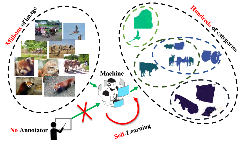
Figure 1: The Large-scale Unsupervised Semantic Segmentation (LUSS) task aims to assign labels from hundreds of categories to pixels from millions of images without the help of human annotation. The model learns to conduct semantic segmentation with Self-Learning.

We propose a benchmark for LUSS task with high-diversity large-scale data, as well as new sufficient evaluation protocols taking into account different perspectives for the LUSS task. Large-scale data with sufficient diversity bring challenges to LUSS, but it also provides the source for obtaining extensive representation cues. Due to insufficient data, a few unsupervised segmentation methods  [28, 29, 30, 31] mainly deal with small data with limited number of categories and small diversity, thus are not suitable for the LUSS task. We present a large-scale benchmark dataset for the LUSS task, namely ImageNet-S, based on the commonly used ImageNet dataset [21] in category representation learning works. We remove the unsegmentable categories, e.g., bookshop, and utilize $919$ categories with about 1.2 million images in ImageNet for training. Then we annotate 40k images in the validation set of ImageNet with precise pixel-level semantic segmentation masks for LUSS evaluation. We also annotate about 9k images in the training set to allow more comprehensive evaluation protocols and exploration of future applications. Based on the more precise re-annotated image-level labels in [32], we enable ImageNet with multiple categories within one image. The ImageNet-S dataset provides large-scale and high-diversity data for fairly LUSS training and sufficient evaluation.

We then present a new method for the LUSS task, including unsupervised representation learning, label generation, and fine-tuning steps. For unsupervised representation learning, we propose 1) a non-contrastive pixel-to-pixel representation alignment strategy to enhance the pixel-level shape representation without hurting the instance-level category representation. 2) a deep-to-shallow supervision strategy to enhance the representation quality of the network mid-level features. The learned representation guarantees the coexistence of shape and category information. We propose a pixel-attention scheme to highlight meaningful semantic regions for label generation, facilitating efficient pixel-level label generation and fine-tuning under a large data scale. Based on the proposed method and ImageNet-S dataset, we study the relation between the proposed LUSS task and some related works (i.e., unsupervised learning [25, 26, 33, 34, 35], weakly supervised semantic segmentation [36, 37, 38], and transfer learning on downstream tasks [27, 5]) and identify the challenges and possible directions of LUSS. In this work, we make two main contributions:

• We propose a new large-scale unsupervised semantic segmentation problem, the ImageNet-S dataset with nearly 50k pixel-level annotated images, 919 categories, and multiple evaluation protocols.

• We present a novel LUSS method containing enhanced representation learning strategies and pixel-attention scheme, and we benchmark related works for LUSS.

2 Related works

2.1 Unsupervised Segmentation

Before the recent advances in deep learning, a plethora of approaches have been developed to segment objects with non-parametric methods (e.g., label transfer [39], matching [40, 41], and distance evaluation [42]) and handcrafted features (e.g., boundary [43] and superpixels [44]). Some unsupervised segmentation (US) methods only focus on segmenting objects but ignore the category, while LUSS cares about object segmentation and classification. Nevertheless, US models can provide prior knowledge to the LUSS model. Numerous data-driven deep learning models have recently been developed for supervised semantic segmentation [1, 2, 4, 5, 45]. Based on pre-trained representations [28, 29, 30, 31], a few unsupervised semantic segmentation (USS) models have been proposed using segment sorting [30], mutual information maximization [28], region contrastive learning [31], and geometric consistency [46]. As the extension of USS, LUSS differs from USS with its large-scale data and categories. However, several issues limit the applicability of the USS to the LUSS task. 1) Existing methods focus on small datasets  [28, 29, 30, 31] and a few (e.g., 20+) easy categories [28] (e.g., sky and ground). Because of the insufficient data, the advantages of unsupervised learning of rich representations from large-scale data are not explored. The challenges of large-scale data (e.g., huge computational cost) are also ignored. 2) Due to the lack of clear problem definition and standardized evaluation, some methods utilize supervised prior knowledge, e.g., supervised pre-trained network weights [46], supervised edge detection [30], and supervised saliency detection [31, 47, 48], making it difficult to evaluate these methods.

2.2 Self-supervised Representation Learning

The LUSS task relies on the semantic features provided by self-supervised learning (SSL). SSL approaches facilitate models learning semantic features with pretext tasks [49, 50, 51, 52], e.g., colorization [53, 54, 55], jigsaw puzzles [56, 57, 58], inpainting [59], adversarial learning [60, 61], context prediction [62, 63], counting [64], rotation predictions [65, 58], cross-domain prediction [66], contrastive learning [67, 68, 25, 26, 24, 69], non-contrastive learning [34, 35, 70], and clustering [71, 72, 33]. We introduce several categories of SSL methods related to the LUSS task.

Contrastive-based SSL. As the core of unsupervised contrastive learning methods [67, 73, 74, 75, 76, 77, 78, 79, 80], instance discrimination with the contrastive loss [81, 82, 83] considers images from different views [24, 69] or augmentations [26, 25] as pairs. In addition, it forces the model to learn representations by pushing “negative” pairs away and pulling “positive” pairs closer. A memory bank [84] is introduced to enlarge the available negative samples for contrastive learning. MoCo [25] stabilizes the training with a momentum encoder. CMC [24] proposes contrastive learning from multi-views, and SimCLR [26] explores the effect of different data augmentations.

Non-contrastive-based SSL. Some non-contrastive approaches [35, 85, 86] maximize the similarity of different types of outputs of the image and avoid negative pairs. BYOL [34] predicts previous versions of its outputs generated by the momentum encoder to avoid outputs collapse to a constant trivial solution. SimSiam [70] applies a stop-gradient operation to avoid collapse. Nevertheless, as the concept of the category is not included in both contrastive and non-contrastive methods, they are less effective for category-related tasks, i.e., instances from the same category not necessarily share similar representations.

Clustering-based SSL. Another line of work introduces a clustering strategy to unsupervised learning [87, 88, 89, 90, 91, 92, 93] that encourages a group of images to have feature representations close to a cluster center. Asano et al. [71] propose simultaneous clustering and representation learning by optimizing the same objective. Li et al. [72] maximize the log-likelihood of the observed data via an expectation-maximization framework that iteratively clusters prototypes and performs contrastive learning. SwAV [33] simultaneously clusters views while enforcing consistency between cluster assignments. Compared to other representation learning methods, the clustering strategy encourages stronger category-related representations with category centroids.

Pixel-level SSL. Some works uses self-supervised learning on the pixel-level instead of image-level to enhance the transfer learning ability to downstream tasks [35, 94, 95]. PixPro [35] applies contrastive learning between neighbour/other pixels and proposes pixel-to-propagation consistency to enhance spatial smoothness. SCRL [94] produces consistent spatial representations of randomly cropped local regions with the matched location. DenseCL [95] chooses positive pairs by matching the most similar feature vectors in two views. Despite the good performance for transfer learning, these methods ignore the category-related representation ability required by the LUSS task.

2.3 Weakly Supervised Semantic Segmentation

Weakly supervised semantic segmentation (WSSS) [96, 97, 98] aims to carry out the task using weak annotations, e.g., image-level labels. WSSS is related to LUSS as both require shape features. However, some modules in typical WSSS methods, e.g., supervised ImageNet_1k pre-trained models [99, 100, 101, 37], image-level ground-truth labels [102, 101], and large network architectures [36, 37], are not applicable to the LUSS tasks. In addition, it is possible to use other alternative WSSS modules e.g., affinity prediction [103, 99, 100], region separation [102, 104], boundary refinement [99, 105], joint learning [106], and sub-category exploration [37], to improve LUSS models.

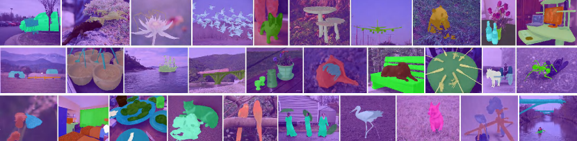
Figure 2: Visualization of the ImageNet-S dataset.

3 Large-scale Unsupervised Semantic Segmentation Benchmark

The LUSS task aims to learn semantic segmentation from large-scale images without direct/indirect human annotations. Given a large set of images, a LUSS model assigns self-learned labels to each pixel of all images. For ease of understanding, we give one of the possible pipelines for LUSS, as shown in Section 4. A LUSS model simultaneously learns category and shape representations from large-scale data without human annotation. The model uses the learned feature representations for label clustering and assignment to get the generated pixel-level labels. Then, the model is fine-tuned on the generated labels to refine the segmentation results. Ideally, label assignment and refining can be implicitly contained in the unsupervised representation learning process.

LUSS faces multiple challenges, e.g., semantic representation learning, category generation under large-scale data, and unsupervised setting. Moreover, the lack of benchmarks limits the development of the LUSS task. As such, we develop a LUSS benchmark with a clear objective, large-scale training data, and comprehensive evaluation protocols.

3.1 Large-scale LUSS Dataset: ImageNet-S

The LUSS task is very challenging as it uses no human-annotated labels for training and requires large-scale data to learn rich representations. In principle, the scale of training images required by LUSS increases with the growth of image complexity, i.e., large category numbers and complex senses require more training data. Existing segmentation datasets can hardly support LUSS due to the large image complexity but small data scale. Some datasets, e.g., PASCAL VOC [10] and CityScapes [7], contain a limited number of images under a few scenes. Other datasets, e.g., ADE20K [8], COCO [107], and COCO-Stuff [11], have complex images with a limited number of samples for each category, which is hard for LUSS models to learn rich representations of complex senses using limited data.

To remedy drawbacks in these datasets, common supervised segmentation approaches [5, 27, 12] fine-tune models pre-trained with the widely used large-scale ImageNet dataset [108, 109, 110, 111]. However, recent research [112, 113] suggested that performance on the ImageNet and downstream datasets is not always consistent due to the inconstancy of data distribution, data domain, and task objective. For LUSS, fine-tuning pre-trained models on downstream datasets complicates the evaluation and leads to possible unfair and biased comparisons. ImageNet has diverse classes, a large data scale, simple images, and sufficient images for each category, making learning rich representations feasible. Thus, ImageNet is widely used by most unsupervised learning methods [26, 33, 35, 24, 25]. However, ImageNet has only image-level annotation, and thus cannot be used for pixel-level evaluation of LUSS. To facilitate the LUSS task, we present a large-scale ImageNet-S dataset by collecting data from the ImageNet dataset [21] and annotating pixel-level labels for LUSS evaluation. We remove the unsegmentable categories, e.g., bookshop, and utilize $919$ categories in ImageNet. As shown in Table I, the ImageNet-S dataset (see Figure 2) is much larger than existing datasets in terms of image amount and category diversity (see Figure 3).

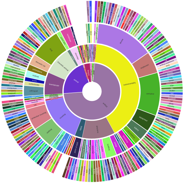
Figure 3: Category structure tree of the ImageNet-S dataset.

3.1.1 Image Annotation.

We annotate the validation/testing sets and parts of the training set in the ImageNet-S dataset for LUSS evaluation. As the ImageNet dataset has incorrect labels and missing multiple categories, we annotate the pixel-level semantic segmentation masks following the relabeled image-level annotations in [32] and further correct the missing and incorrect annotations. The objects indicating the image-level labels are annotated, and other parts are annotated as the ‘other’ category. ‘Other’ means the categories are not frequently appeared in the dataset or the surrounding environment. For validation/testing sets, we annotate all objects within the $919$ selected categories. The parts that are difficult to distinguish are marked as ‘ignore’, which will not be used for evaluation. For the training set, we randomly pick ten images for each category and annotate objects corresponding to that category while other objects belonging to the $919$ categories are labeled with ‘ignore’.

TABLE I: Categories and number of images comparison between the ImageNet-S dataset and existing semantic segmentation datasets.

Dataset	category	train	val	test
PASCAL VOC 2012 [10]	$20$	$1464$	$1449$	$1456$
CityScapes [7]	$19$	$2975$	$500$	$1525$
ADE20K [8]	$150$	$20210$	$2000$	$3000$
ImageNet-S50	$50$	$64431$	$752$	$1682$
ImageNet-S300	$300$	$384862$	$4097$	$9088$
ImageNet-S	$919$	$1183322$	$12419$	$27423$

Semantic segmentation mask annotation. Given the categories of an image, the annotator is asked to annotate the corresponding regions and assign the correct categories. The selected $919$ categories in the ImageNet-S dataset have high diversity. Some instances cannot be easily distinguished even with given categories, e.g., two breeds of dogs and uncommon things. To reduce the difficulty for annotators to identify categories, we splice four images with the same category into a four-square image. In this case, annotators can easily distinguish the common categories in the four-square image. For images with multiple complex categories, several groups of images containing the required categories are provided to help annotators identify categories. Since the categories in the ImageNet-S dataset follow a tree-like structure (see Figure 3), different annotators are given images from different subsets of the Word-Tree to further reduce the annotation difficulty. Images with a resolution below $1000$ $\times$ $1000$ are resized to $1000$ $\times$ $1000$. The annotator draws polygonal masks to the category-related regions with about $400$ to $500$ points on the contour for each image. Annotating on resized high-resolution images results in precise pixel-level semantic segmentation masks.

TABLE II: The number of categories in each image in the ImageNet-S dataset.

	Number of images
	val set			test set
Categories in each image	$1$	$2$	$>$2	$1$	$2$	$>$2
ImageNet-S50	$745$	$7$	$0$	$1676$	$6$	$0$
ImageNet-S300	$3971$	$118$	$8$	$8815$	$264$	$9$
ImageNet-S	$11294$	$954$	$171$	$25133$	$1938$	$352$

\begin{overpic}[width=203.80193pt]{image_val_counts.pdf} \put(61.0,36.5){val and test set} \put(-8.0,16.0){\rotatebox{90.0}{number}} \end{overpic}

(a) Number of images per class.

\begin{overpic}[width=203.80193pt]{image_train_semi_counts.pdf} \put(52.0,49.6){anno-training set} \end{overpic}

(b) Number of images per class.

\begin{overpic}[width=203.80193pt]{pixel_val_counts.pdf} \put(60.5,37.6){val and test set} \put(-8.0,16.0){\rotatebox{90.0}{number}} \put(10.0,54.0){$\times 10^{7}$} \end{overpic}

(c) Number of pixels per class.

\begin{overpic}[width=203.80193pt]{pixel_train_counts.pdf} \put(51.0,38.2){anno-training set} \put(9.0,52.0){$\times 10^{6}$} \end{overpic}

(d) Number of pixels per class.

Figure 4: Instance-level/pixel-level number distribution among categories of the ImageNet-S dataset, i.e., the number of images/pixels per class.

Labeling process. The annotation team for this dataset contains an organizer, four quality inspectors, and $15$ annotators. We introduce the labeling process as follows:

Step 1. Annotators were instructed on how to annotate labels. Then annotators were asked to annotate a group of randomly picked images following instructions. Quality inspectors checked these annotated images, and failure cases were corrected and shown as examples to all annotators.

Step 2. The annotators were divided into several groups, and each group has a group leader. The organizer then assigned images to each group of annotators. After annotating the images, the group leader summarized all annotations and checks the annotation quality. Other annotators checked the annotations from the group leader in the group.

Step 3. The checked annotations were then given to the quality inspectors. Quality inspectors checked the annotations and give feedback regarding the failure cases. Common failure cases and corresponding explanations are sent to all groups to improve the annotation quality of the following images.

Step 4. The organizer then sampled images and checked the corresponding annotations to ensure the annotation quality.

Correct missing/incorrect labels. During the labeling process, we observed that there were still some missing and incorrect image-level annotations in [32] due to the high diversity and large-scale properties of ImageNet. Therefore, we presented several schemes to correct labels as much as possible: 1) We found that some categories are related to each other, e.g., the spider and spider web usually appear in the same image. Based on the initial human-observed missing categories, we double-checked images whose categories are related to other categories. 2) We used supervised image-level classifiers, e.g., Swin transformer [114] and Res2Net [110], to help find missing categories by checking the labels predicted with high confidence but not in the ground-truth. With these schemes, we managed to correct $296$ mislabeled images and find $942$ images with missing labels.

3.1.2 Statistics and distribution.

Image numbers. As shown in Table I, after removing the unsegmentable categories in the ImageNet dataset, e.g., bookshop, valley, and library, the ImageNet-S dataset contains $1183322$ training, $12419$ validation, and $27423$ testing images from $919$ categories. Many existing self-supervised representation learning methods [25, 35] are trained with the ImageNet dataset. For a fair comparison, we use the full ImageNet dataset that contains $1281167$ training images for unsupervised representation learning and utilize the ImageNet-S training set for other processes in LUSS. We annotate $39842$ validation/testing images and $9190$ training images with precise pixel-level masks, and some visualized annotations are shown in Figure 2. Our pixel-level labeling enables the ImageNet-S dataset with multiple labels in each image. Table II gives the number of categories per image in the ImageNet-S validation/testing sets. A majority of images contain one category, and 8.6% of images have more than one category. ImageNet-S has simpler images and more categories than existing semantic segmentation datasets, which is suitable for the LUSS task considering the difficulty caused by no human annotation and large image and category numbers.

Category distribution. As shown in Figure 3, categories in the ImageNet-S dataset show a tree-like structure as they are extracted from the Word-Tree [21]. Figure 4 shows the image-level and pixel-level number distribution among categories of the ImageNet-S dataset, i.e., the number of images/pixels per class. The training set and validation/testing sets have similar distributions. The number of images for most categories is balanced, while the number of pixels per category presents the long-tail distribution. The imbalanced pixel-level category distribution may introduce new challenges that are not considered in the image-level representation learning. Compared to the original ImageNet dataset with a similar number of images for each category in the validation set, the relabeled ImageNet-S validation/testing sets presents a more unbalanced number of images over categories.

\begin{overpic}[width=368.57964pt]{luss919_mask_size_val.pdf} \put(55.0,42.0){small} \put(55.0,36.9){medium-small} \put(55.0,32.2){medium-large} \put(55.0,26.8){large} \put(97.0,0.6){\%} \put(-5.0,20.0){\rotatebox{90.0}{frequency/\%}} \end{overpic}

(a) Distribution of validation and testing set.

\begin{overpic}[width=368.57964pt]{luss919_mask_size_train.pdf} \put(55.0,42.0){small} \put(55.0,36.9){medium-small} \put(55.0,32.2){medium-large} \put(55.0,26.8){large} \put(97.0,0.6){\%} \put(-5.0,20.0){\rotatebox{90.0}{frequency/\%}} \end{overpic}

(b) Distribution of the annotated training images set.

Figure 5: Distribution of object size in the ImageNet-S dataset. The object size is defined as the ratio of object size to the image size.

Object size. As it is more difficult to segment smaller objects, we divide objects into groups, i.e., small (0%-5%), medium-small (5%-25%), medium-large (25%-50%), and large object size (50%-100%), according to the ratio of object size to the image size. The object size distribution shown in Figure 5 indicates that most objects are relatively small.

Position distribution. We superimpose segmentation masks from the validation and testing sets to analyze the position distribution of semantic objects in the dataset, as shown in Figure 6 (top). The objects in ImageNet-S tend to be in the centre of the image, which explains the effectiveness of the central crops strategy of existing self-supervised methods [26, 25]. We also superimpose the boundary of objects, as shown in Figure 6 (down). It shows that objects cover almost all areas instead of only the central area of images. In addition, we compare the distributions of our dataset with COCO [107] and Open Images [115] datasets in Figure 6. Our dataset and the other two datasets have similar distributions. The centre-skewed distribution is observed for all datasets, and we assume that humans might tend to record more centre-biased images. Interestingly, the distribution map of ImageNet-S is almost identical to the Open Images dataset, famous for its real-life property.

Annotation consistency. We validate the annotation quality by evaluating the annotation consistency of different people. We have asked four annotators to annotate the same 100 randomly picked images, respectively. Based on four sets of samples, we evaluate the average metrics between each pair using mask mIoU and boundary mIoU, as shown in Table III. The mask mIoU is 98.7%, showing a high annotation consistency. With a small d of 2%, the boundary mIoU still has 92.4%, indicating high constant boundary annotations. We visually observe that the main annotation differences are in the boundary regions. By comparing objects of different sizes, smaller objects have lower annotation consistency since the boundary regions occupy a larger proportion of the annotation mask in smaller objects.

TABLE III: The consistency among four annotators using $100$ randomly picked images. The $d$ indicates the pixel distance as in [116].

Metrics	$d$	All	S.	M.S.	M.L.	L.
Boundary mIoU[116]	2%	92.4	91.0	91.5	92.7	93.4
	3%	94.8	92.6	93.9	95.1	95.5
	4%	95.9	93.2	95.1	96.2	96.5
Mask mIoU	-	98.7	93.4	97.1	99.0	99.3

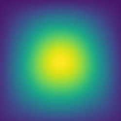
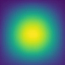
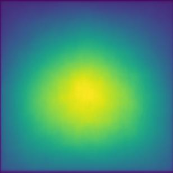
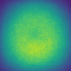
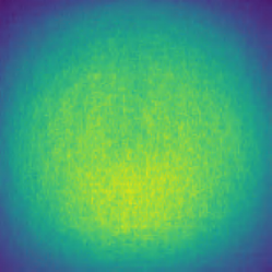
ImageNet-S	Open Images	COCO

Figure 6: Position distribution comparison among datasets: (top) the position distribution for segmentation masks, (down) the position distribution for mask boundaries.

\begin{overpic}[width=390.25534pt]{figures/lsusss.pdf} \put(3.5,4.0){Large-scale data} \put(27.0,2.5){Supervision} \put(37.5,20.2){Self-supervision} \put(54.5,14.0){Clustering} \put(68.7,15.0){Pseudo} \put(68.7,12.5){Labels} \put(63.0,5.2){Fine-tuning} \put(83.3,3.4){Semantic seg.} \end{overpic}

Figure 7: The pipeline of our method for the LUSS task.

ImageNet-S-50/300 under a limited budget. To facilitate the research under a low computational budget, we develop two subsets containing $50$ and $300$ categories, namely ImageNet-S₅₀ and ImageNet-S₃₀₀. Considering the difficulty of the LUSS task, we choose $50$ distinguishable categories in daily life for ImageNet-S₅₀. The ImageNet-S₃₀₀ is composed of ImageNet-S₅₀ and $250$ randomly sampled categories. The number of images in ImageNet-S₅₀ and ImageNet-S₃₀₀ are shown in Table I. Even the ImageNet-S₅₀ subset has more images than most semantic segmentation datasets.

3.2 Evaluation

3.2.1 Evaluation Protocols

Due to the lack of ground-truth (GT) labels during training, LUSS models cannot be directly evaluated as in the supervised setting. We present three evaluation protocols for LUSS, including the fully unsupervised evaluation, semi-supervised evaluation, and distance matching evaluation.

Fully unsupervised protocol. The fully unsupervised evaluation protocol requires no human-annotated labels during training and only needs the validation/testing set for evaluation. Unlike the supervised tasks, categories are generated by the model in the LUSS task, which needs to be matched with GT categories during evaluation. We present the default image-level matching scheme, while a more effective matching scheme should improve LUSS evaluation performance. Suppose the set for matching (normally validation set) has $N$ images and $C$ categories. The number of categories is implicitly contained in the training dataset as the dataset has $C$ major categories. We assume the unsupervised model should learn to generate more than $C$ categories from the dataset during training. The default image-level matching scheme only matches $C$ generated categories with $C$ ground-truth categories. Given the image set $\mathbf{D}=\{\mathbf{D}_{k},k\in[1,N]\}$ with GT labels $\mathbf{G}=\{\mathbf{G}_{k},k\in[1,N]\}$ and predicted labels $\mathbf{P}=\{\mathbf{P}_{k},k\in[1,N]\}$, where $\mathbf{G}_{k}$ and $\mathbf{P}_{k}$ are the GT and predicted category sets of the image $\mathbf{D}_{k}$. We calculate the matching matrix $\mathbf{S}\in\mathbb{R}^{C\times C}$ between generated and GT categories, in which $\mathbf{S}_{ij}$, representing the matching degree between the $i$-th generated category and the $j$-th GT category, is larger when two categories are more likely to be the same category:

$$\mathbf{S}_{ij}=\sum_{k=1}^{N}\mathbb{I}\{(i,j)\in\mathbf{P}_{k}\times\mathbf{G}_{k}\},$$ (1)

where $\mathbf{P}_{k}\times\mathbf{G}_{k}$ is the Cartesian product of $\mathbf{P}_{k}$ and $\mathbf{G}_{k}$, and the indicator $\mathbb{I}$ equals $1$ when $(i,j)$ belongs to $\mathbf{P}_{k}\times\mathbf{G}_{k}$. With the matching matrix $\mathbf{S}\in\mathbb{R}^{C\times C}$, we find the bijection $\mathbf{f}:i\mapsto j$ between generated and GT categories using the Hungarian algorithm [117] to maximize $\sum_{i=1}^{C}\mathbf{S}_{i,\mathbf{f}(i)}$. We observe that there are failed matching cases and some generated categories are not in the ground-truth categories, indicating the limit of our baseline matching method. We expect future works to propose more effective matching methods to solve this problem.

Semi-supervised protocol. We can conduct semi-supervised fine-tuning to evaluate LUSS models as we annotate about 1% of training images with pixel-level labels. The semi-supervised evaluation protocol requires fine-tuning the trained LUSS models with human-labeled training images. Therefore, this protocol does not need matching generated and GT category. Also, this protocol is suitable for real-world applications where a small part of images are labeled and many images are unlabeled.

Distance matching protocol. In the distance matching evaluation protocol, we directly get the embeddings of GT categories with the pixel-level labeled training images and match them with embeddings in validation/testing sets to assign labels. Specifically, for pixels with the same category in an image (including the ‘other’ category), we get the averaged embeddings and the corresponding label in the training set. Then we infer the segmentation masks of the validation/testing sets using the k-NN classifier [84]. For each pixel embedding in the validation/testing sets, we find the top-$k$ similar embeddings in the training set and the corresponding labels. The assigned label of each pixel is determined by the voting among these $k$ labels.

3.2.2 Evaluation metrics

We use the mean intersection over union (mIoU), boundary mIoU (b-mIoU), image-level accuracy (Img-Acc), and F-measure ($F_{\beta}$) as the evaluation metrics for the LUSS task. During the evaluation, all images are evaluated with the original image resolution. mIoU and b-mIoU are comprehensive evaluation metrics, while Img-Acc and $F_{\beta}$ explain the performance from category and shape aspects. We give the implementation details of these evaluation metrics in the supplementary.

Mean IOU. Similar to the supervised semantic segmentation task [10, 8], we utilize the mIoU metric to evaluate the segmentation mask quality. Apart from the major categories, the ‘other’ category is also considered to get mIoU.

Boundary mean IoU. Unlike the mask mIoU above that measures all object regions, the boundary mean IoU (b-mIoU) [116] focuses on the boundary regions. We use the boundary mIoU to measure the semantic segmentation quality of boundary regions. According to the segmentation consistency analysis in Section 3.1.2, we use $d=3\%$ for boundary IoU [116].

Image-level accuracy. The Img-Acc can evaluate the category representation ability of models. As many images contain multiple labels, we follow [32] and treat the predicted label as correct if the predicted category with the largest area is within the GT label list.

F-measure. In addition to category-related representation, we utilize $F_{\beta}$ to evaluate the shape quality [118], which ignores the semantic categories. We treat major categories as the foreground category and the ‘other’ category as the background category.

4 A LUSS Method

4.1 Overview

We summarize the main challenges of the LUSS task: 1) The model should learn category-related representations without image-level label supervision. 2) Extracting a semantic segmentation mask requires the model to learn shape representations. 3) Shape and category representations should coexist with minimal conflict. 4) With learned representations, the model should assign self-learned labels to each pixel in the image with high efficiency. 5) The large-scale training data helps to learn rich representations in an unsupervised learning manner but inevitably causes a large amount of training cost, which requires improving the training efficiency.

Considering the above challenges, we propose a new method for LUSS, namely PASS, (see Figure 7), containing four steps. 1) A randomly initialized model is trained with self-supervision of pretext tasks to learn shape and category representations. After representation learning, we obtain the features set for all training images. 2) We then apply a pixel-attention-based clustering scheme to obtain pseudo categories and assign generated categories to each image pixel. 3) We fine-tune the pre-trained model with the generated pseudo labels to improve the segmentation quality. 4) During inference, the LUSS model assigns generated labels to each pixel of images, same to the supervised model. Noted that the pipeline in our method is not the only option, and other pipelines are also encouraged for the LUSS task. We now give a detailed introduction of each step as follows. Some frequently used symbols are listed in Table IV for easier understanding.

4.2 Unsupervised Representation Learning

For the first step in our LUSS method, a randomly initialized model, e.g., ResNet, is trained with self-supervision of pretext tasks to learn semantic representations. The LUSS task requires category-related representation to distinguish scenes from different classes and shape-related representation to form the shape of objects. Prior works have made many efforts to learn image-level category-related representation or pixel-level representation [35, 94, 95]. However, the image-level methods often ignore shape-related features. The pixel-level methods focus on the transfer learning performance on supervised downstream tasks. As observed by [119], the performance of most downstream tasks relies on low-level feature from the early stage of the network. Thus, pixel-level methods that perform well on downstream tasks may not learn high-level semantic features with category and shape information.

To obtain a powerful representation for LUSS, we present two self-supervised learning strategies to enhance both category and shape representation, including 1) a non-contrastive pixel-to-pixel representation alignment strategy to enhance the pixel-level shape-related representation without hurting the instance-level category representation. 2) a deep-to-shallow supervision strategy to enhance the representation quality of mid-level features of the network.

\begin{overpic}[width=433.62pt]{p2p.pdf} \put(38.8,27.0){\rotatebox{270.0}{Network}} \put(52.0,24.0){\rotatebox{270.0}{$\mathbf{M_{p}}$}} \put(72.0,33.0){\rotatebox{270.0}{$\mathbf{P}$}} \put(64.0,20.0){non-contrastive} \put(68.0,17.0){alignment} \put(45.0,27.0){$\mathbf{\tilde{z}}_{1}$} \put(45.0,13.0){$\mathbf{\tilde{z}}_{2}$} \put(58.0,27.0){$\mathbf{\tilde{v}}_{1}$} \put(58.0,13.0){$\mathbf{\tilde{v}}_{2}$} \put(87.0,39.0){$\mathbf{P}(\mathbf{\tilde{v}}_{1})$} \put(88.0,5.0){$\mathbf{\tilde{v}}_{2}$} \put(90.0,22.0){$L_{s}$} \end{overpic}

Figure 8: Illustration of non-contrastive pixel-to-pixel representation alignment. $\mathbf{M_{p}}$ is the projection layer that ensures less interference of pixel-level representation to the category representation. $\mathbf{P}$ is a pixel-level predictor for the asymmetric loss.

TABLE IV: Definition of frequently used symbols.

Symbols	Dimensions/Type	Meaning
$\mathbf{z}$	$L\times H\times W$	output feature of one image.
$\mathbf{z}_{k}$	$L\times H\times W$	output feature of the $k$-th image.
$\mathbf{q}_{k}$	$(C+1)\times H\times W$	pixel-level pseudo labels of the $k$-th image.
$\mathbf{y}_{k}$	$(C+1)\times H\times W$	pixel-level GT labels of the $k$-th image.
$C$	scalar	number of major categories.
$L$	scalar	number of dimensions of output feature.
$H$	scalar	height of output feature.
$W$	scalar	width of output feature.
$N$	scalar	number of images.
$\mathbb{P}$	operation	global average pooling over spatial dimensions.

Non-contrastive pixel-to-pixel representation alignment. Pixel-level shape-related representation aims to enhance the feature discrimination ability in pixel-level, i.e., pixels within the same category or from the same image position of different views should have consistent representations, and vice versa. We observe that most existing pixel-level methods perform worse than image-level methods on the LUSS task. We argue existing pixel-level methods focus too much on the pixel-level distinction, thus resulting in semantic variation among pixels within the same instance. To avoid the side-effect of pixel-level representation to instance-level category representation, we propose a non-contrastive pixel-to-pixel representation alignment strategy that aligns the features from the same image position of different views but avoids pushing features from other positions away.

As shown in Figure 8, given the feature pair predicted from two views of the image, we extract features $(\mathbf{\tilde{z}}_{1},\mathbf{\tilde{z}}_{2})$ of the overlapped pixels and get the pixel-level embedding pairs ($\mathbf{\tilde{v}}_{1}$,$\mathbf{\tilde{v}}_{2}$) by the projection $\mathbf{\tilde{v}}=\mathbf{M_{p}(\mathbf{\tilde{z}})}$, where $\mathbf{M_{p}}$ is the pixel-level multi-layer projection (MLP) layer composed of the two conv1$\times$1 layers and activation layers. We show in Section 5.3.1 that the projection $\mathbf{M_{p}(\tilde{z})}$ ensures less interference of pixel-level representation to the category representation. We utilize the pixel-to-pixel alignment to align the overlapped pixel-level embeddings from two views using the asymmetric loss:

$$L_{P2P}=L_{s}(\mathbf{P}(\mathbf{\tilde{v}}_{1}),\cancel{\mathbf{G}}(\mathbf{\tilde{v}}_{2}))+L_{s}(\cancel{\mathbf{G}}(\mathbf{\tilde{v}}_{1}),\mathbf{P}(\mathbf{\tilde{v}}_{2})),$$ (2)

where the projection $\mathbf{P}$ is a pixel-level MLP predictor, $\cancel{\mathbf{G}}$ is the stop gradient operation to avoid the collapse of predictor [70], and $L_{s}$ is a cosine similarity loss. The proposed non-contrastive pixel-to-pixel alignment forms a robust pixel-level representation across different views and maintains the category representation ability.

Deep-to-shallow supervision. The quality of low/mid-level representation, i.e., representation in early network layers, is proven critical to vision tasks [120, 113]. Islam et al. [120] reveal representations with rich low/mid-level semantics in early layers result in quick adaptation to a new task. Similarly, Kotar et al. [113] show the benefit of high-quality low-level features learned with contrastive-based methods. Most existing works optimize mid-level representation by the indirect gradient back-propagation from the high-level of the network [25, 26, 72, 33]. We observe that directly applying low/mid-level features for representation learning leads to sub-optimal performance as these features lack semantics. Therefore, we propose a deep-to-shallow supervision strategy to enhance the representation of low/mid-level features with the guidance of high-quality high-level features.

As shown in Figure 9, given two views augmented from one image, we obtain the feature pairs $(\mathbf{z}_{1}^{(s)},\mathbf{z}_{2}^{(s)})$ from the $s$ stage of the network. We mainly explore the effect of deep-to-shallow supervision on image-level for simplicity. Given a network with four stages, the image-level embeddings used for deep-to-shallow supervision are obtained as follows:

$$\mathbf{u}_{i}^{(s)}=\begin{cases}\mathbf{M}^{s}_{I}(\mathbb{P}(\mathbf{z}_{i}^{(s)}))&s=4;\\ \mathbf{M}^{s}_{I}(\mathbb{P}(\mathbf{M}_{K}^{s}(\mathbf{z}_{i}^{(s)})))&s<4,\end{cases}$$ (3)

where $\mathbb{P}$ is the global average pooling operation in the spatial dimension, $\mathbf{M}_{I}^{s}$ and $\mathbf{M}_{K}^{s}$ are the image-level/pixel-level MLP layers of the stage $s$, respectively. We observe that directly pooling the mid-level features causes the representation collapse, and adding $\mathbf{M}_{K}^{s}$ avoids this problem. In the deep-to-shallow supervision strategy, the embeddings from the last stage of one view are used to supervise embeddings of another view from all stages:

$$L_{D2S}=\frac{1}{|S|}\sum_{j}^{j\in S}{L_{I}(\mathbf{u}_{1}^{(4)},\mathbf{u}_{2}^{(j)})}+\frac{1}{|S|}\sum_{j}^{j\in S}{L_{I}(\mathbf{u}_{2}^{(4)},\mathbf{u}_{1}^{(j)})},$$ (4)

where $S$ is a set containing stages used for deep-to-shallow supervision, and $L_{I}$ is the image-level loss. $L_{I}$ can be multiple definitions, and we use the clustering loss [33] as $L_{I}$ in our work.

Training loss for representation learning. Our proposed pixel-to-pixel alignment and deep-to-shallow supervision can cooperate with existing methods to improve representation quality. The summarized loss for the unsupervised representation learning step is written as:

$$L_{sum}=L_{P2P}+L_{D2S}+L_{e},$$ (5)

where $L_{e}$ is the loss of existing methods, e.g., SwAV [33] and PixelPro [35].

\begin{overpic}[width=433.62pt]{d2s.pdf} \put(95.0,4.0){$\mathbf{u}_{2}^{(4)}$} \put(77.0,4.0){$\mathbf{u}_{2}^{(3)}$} \put(60.0,4.0){$\mathbf{u}_{2}^{(2)}$} \put(45.0,4.0){$\mathbf{u}_{2}^{(1)}$} \put(95.0,42.0){$\mathbf{u}_{1}^{(4)}$} \put(77.0,42.0){$\mathbf{u}_{1}^{(3)}$} \put(60.0,42.0){$\mathbf{u}_{1}^{(2)}$} \put(45.0,42.0){$\mathbf{u}_{1}^{(1)}$} \end{overpic}

Figure 9: Illustration of deep-to-shallow supervision. Purple lines denote the supervisions using loss $L_{I}$. $\mathbf{M}_{I}^{s}$ and $\mathbf{M}_{K}^{s}$ are omitted for simplicity.

4.3 Pixel-label Generation with Pixel-Attention

After representation learning, we obtain the features set $\mathbf{Z}=\{\mathbf{z}_{k}\in\mathbb{R}^{L\times H\times W},k\in[1,N]\}$ for all training images, where $N$ is the number of images, $L$, $H$, and $W$ are the number of dimensions, height, and width of the output features. We cluster $\mathbf{Z}$ to obtain $C$ generated categories and assign generated categories to each pixel. A straightforward way for label generation is to cluster embeddings of all pixels in the training set, which is too costly due to the large-scale data in LUSS, e.g., clustering training images of ImageNet-S at pixel-level with $7\times 7$ resolution requires about $114$ hours. An alternative is to use image-level features pooled on the spatial dimension to save clustering costs. However, many irrelevant embeddings are included in the pooled features, hurting the clustering quality.

We observe that the learned features tend to focus on the regions with more semantic meanings, i.e., pixels with more useful semantic information contribute more to the convergence of unsupervised representation learning. Based on this observation, we propose a pixel-attention scheme to highlight meaningful semantic regions, facilitating the pixel-level label generation with image-level features. Specifically, we add a pixel-attention head at the output of models and fine-tune it with representation learning losses to filter out the less semantic meaningful regions. Filtering features with pixel-attention reduces noise in the pooled image-level embeddings, improving the clustering quality. Also, the pixel-attention separates the semantic regions with less meaningful regions, generating more accurate object shapes during pixel-level label generation. We give the implementation detail of pixel-attention in fine-tuning and label generation steps.

Fine-tuning pixel-attention. Given the feature $\mathbf{z}$ of one image predicted by the model, representation learning methods [33, 25], calculate losses with the pooled feature embeddings $\mathbf{M}_{I}(\mathbb{P}(\mathbf{z}))$, where $\mathbf{M}_{I}$ is the image-level MLP layer. The pooling operation treats all pixels equally, inevitably introducing noises to image-level embeddings as not all pixels represent meaningful semantics. Our pixel-attention is defined as:

$$\mathbf{c(z)}=\sigma(\mathbf{M}_{A}(\|\mathbf{z}\|)+\theta),$$ (6)

where $\mathbf{M}_{A}$ is the pixel-level MLP layer, $\theta\in\mathbb{R}^{L}$ are learnable parameters initialized with zero, $\sigma$ is a sigmoid function to restrict output attention value, and $\|\mathbf{z}\|$ is the L2 normalization operation applied on the channel dimension of feature $\mathbf{z}$. Each channel of $\mathbf{z}$ has a corresponding pixel-attention map. We multiply the pixel-attention to feature $\mathbf{z}$ and obtain the pixel-attention enhanced image-level embedding $\mathbf{\hat{v}=M}_{I}(\mathbb{P}(\mathbf{c(z)\cdot\|z}\|))$. During fine-tuning, we detach gradients to the network and fine-tune the pixel-attention module by optimizing representation loss calculated from $\mathbf{\hat{v}}$. We observe that fine-tuning pixel-attention module with clustering loss [33] results in decent shape-related pixel-attention results (see Figure 10).

Figure 10: Visualization of pixel-attention maps of different channels. Most pixel-attention maps highlight the semantic regions, while a few channels highlight the background regions.

Label generation with pixel-attention. Based on pixel-attention $\mathbf{c(z)}$, we obtain the pixel-attention enhanced image-level feature $\mathbf{\hat{Z}}=\{\mathbf{\hat{Z}}_{k}\in\mathbb{R}^{L},k\in[1,N]\}$, where $\mathbf{\hat{Z}}_{k}=\mathbb{P}(\mathbf{c(z)}_{k}\cdot\mathbf{z}_{k})$. We conduct the k-means clustering over $\mathbf{\hat{Z}}$ to generate the cluster center $K\in\mathbb{R}^{L\times C}$ of $C$ categories. With the generated categories, we need to assign pixel-level pseudo labels $\mathbf{Q}=\{\mathbf{q}_{k}\in\mathbb{R}^{(C+1)\times H\times W},k\in[1,N]\}$ to images. We show in Figure 10 the fine-tuned pixel-attention highlights semantic regions of images. Therefore, we extract regions with rich semantic information based on pixel-attention:

$$\mathbf{d(z)}=\begin{cases}0&\frac{1}{L}\sum_{i}^{0\leq i<L}\mathbf{c(z)}_{i}<\tau;\\ 1&\frac{1}{L}\sum_{i}^{0\leq i<L}\mathbf{c(z)}_{i}\geq\tau,\end{cases}$$ (7)

where $\tau$ is a pre-defined threshold between major categories and the ‘other’ category, and regions with pixel-attention below $\tau$ are traded as the ‘other’ category. For each pixel in the region of major categories, we assign one category in the cluster center $K$ that has the minimal distance to the feature embedding of the pixel.

4.4 Fine-tuning and Inference

During the fine-tuning step, we load the weights pre-trained with representation learning and add a conv 1$\times$1 layer with $L\times(C+1)$ channels as the segmentation head. The output features $\mathbf{Y}=\{\mathbf{y}_{k}\in\mathbb{R}^{(C+1)\times H\times W},k\in[1,N]\}$ from this head are supervised with $\mathbf{Q}$ to fine-tune the model using cross-entropy loss. During inference, the LUSS model acts like a fully supervised semantic segmentation model. For each pixel embedding $\mathbf{w}\in\mathbb{R}^{C+1}$ in $\mathbf{y}_{k}$, we get the segmentation labels as follow:

$$\mathbf{w}={\arg\max}_{i\in[1,C+1]}(\mathbf{w}_{i}).$$ (8)

5 Experiments and Analysis

5.1 Implementation Details

Training details on the representation learning step. We use ResNet-18 network for the ImageNet-S₅₀ dataset and utilize ResNet-50 for ImageNet-S₃₀₀ and ImageNet-S datasets. For a fair comparison, all networks are trained with a mini-batch size of $256$ for $200$ epochs in ImageNet-S₅₀ and $100$ epochs in ImageNet-S₃₀₀/ImageNet-S.

Our method cooperates with the image-level method SwAV [33] and the pixel-level method PixelPro [35]. Following SwAV [33], a LARS optimizer is used to update the network with a weight decay of 1e-6 and a momentum of 0.9. The initial learning rate is 0.6 and gradually decays to 6e-6 with the cosine learning rate schedule. For ImageNet-S₃₀₀ and ImageNet-S datasets, to make a fair comparison with other methods, we only use two crops with the size of 224$\times$224 for training, and the multi-crop training strategy [33] is not applied. Same as SwAV, a queue with the length of $3840$ is used beginning from $15$ epochs, and the prototypes for clustering are frozen before $5005$ iterations. When training on ImageNet-S₅₀, the queue is set to 2048, and prototypes are frozen before $1001$ iterations to ease the convergence. We use the multi-crop training strategy containing 6 crops with the size of 96$\times$96 and two crops with the size of 224$\times$224 for training on ImageNet-S₅₀. When cooperating with PixelPro [35], the training schemes are consistent with the official setting. We train the network with the initial learning rate of 1.0 using a LARS optimizer. After five warm-up epochs, the learning rate gradually decays to 1e-6 with the cosine learning rate schedule.

Training details on the fine-tuning step. To generate pixel-level labels, we first fine-tune the pixel-attention module for $20$ epochs while fixing the model parameters trained in the unsupervised representation learning step. We apply the clustering loss [33] to fine-tune the pixel-attention module by default. The training strategy remains the same as that in the representation learning step.

The representation learning losses are removed in the fine-tuning step, and an extra cross-entropy loss is added to supervise the segmentation head. We load the model weights pre-trained on the representation learning step and fine-tune them for $20$ epochs. We train the network using a LARS optimizer with a weight decay of 1e-6, a mini-batch size of 256, and a momentum of 0.9. The initial learning rate is 0.6 and gradually decays to 6e-6 with the cosine learning rate schedule.

TABLE V: Comparison of our proposed LUSS method and existing USS methods on the ImageNet-S dataset using the fully unsupervised evaluation protocol. Test mIoU under different object sizes are provided. † means train model for $200$ epochs from scratch. PASS_s/p denotes using SwAV [33] and PixelPro [35] as the $L_{e}$ in (5), respectively. S means the method use saliency maps. I means initialization with supervised ImageNet_1k pre-training. By default, the ‘other’ category is used to calculate mIoU and b-mIoU. We also give the performance without using the ‘other’ category in the supplementary.

LUSS	Pior	mIoU		b-mIoU		Img-Acc		Fβ		mIoU				b-mIoU
		val	test	val	test	val	test	val	test	S.	M.S.	M.L.	L.	S.	M.S.	M.L.	L.
ImageNet-S50
MDC[88, 46]	-	4.0	3.6	1.4	1.2	14.9	13.4	31.6	31.3	0.4	2.6	3.8	4.9	0.2	1.1	1.4	1.5
MDC[88, 46]	I	14.6	14.3	3.1	3.1	44.8	40.8	33.2	32.6	2.6	10.9	14.6	19.1	0.9	2.2	3.2	4.7
PiCIE[46]	-	5.0	4.5	1.8	1.6	15.8	14.0	14.6	32.2	0.2	3.1	5.0	5.3	0.2	1.2	1.7	1.9
PiCIE[46]	I	17.8	17.6	3.7	4.0	45.0	44.0	32.1	31.6	4.4	13.1	20.1	23.1	1.0	2.7	4.4	5.8
MaskCon[31]	S	24.6	24.2	15.6	15.1	47.9	47.6	65.7	66.2	12.2	25.6	24.7	20.4	10.1	17.0	14.5	10.6
MaskCon[31]†	S	13.9	10.5	8.5	10.5	30.2	22.4	62.6	62.3	2.5	2.1	1.7	1.7	2.4	6.3	6.5	5.7
PASSs	-	29.2	29.3	7.6	7.4	66.2	65.5	49.0	49.0	6.6	25.0	33.2	32.6	3.3	6.2	8.1	9.5
PASSp	-	32.4	32.0	7.2	7.2	62.9	64.1	48.7	47.9	9.7	26.2	36.5	40.5	5.1	5.8	7.8	10.4
PASSp+ RC [118]	S	42.6	42.1	17.5	17.7	58.8	61.8	62.1	61.3	17.0	38.6	45.5	43.7	11.2	17.2	19.0	17.1
PASSp+ Sal	S	43.3	42.3	20.4	20.2	64.6	65.2	70.0	69.9	19.0	41.7	45.1	38.3	14.7	22.6	20.6	15.3
ImageNet-S300
PASSp	-	16.6	16.0	4.4	4.2	34.7	32.8	34.4	34.3	2.8	12.0	16.4	21.7	1.4	3.2	3.9	6.4
PASSs	-	18.0	18.1	5.2	5.2	43.9	42.6	47.6	47.5	4.2	13.6	19.5	23.5	2.1	4.2	5.5	7.1
ImageNet-S
PASSp	-	7.3	6.6	2.4	2.1	19.9	18.0	34.8	34.6	1.3	4.6	7.1	8.4	0.6	1.5	2.1	2.8
PASSs	-	11.5	11.0	3.8	3.5	24.0	22.3	37.1	36.9	2.4	8.3	11.9	13.4	1.3	3.0	3.8	4.3

5.2 Comparison with USS Methods

In this section, we evaluate the performance of the proposed LUSS method on the ImageNet-S dataset using the fully unsupervised evaluation protocol. Table V shows our method achieves reasonable performance on the large-scale data. The visualization shown in Figure 11 indicates that unsupervised semantic segmentation with the large-scale dataset is achievable.

Comparison with unsupervised semantic segmentation methods. Existing unsupervised semantic segmentation (USS) methods are designed for relatively small scale data, thus cannot be directly used on the full-scale ImageNet-S dataset due to the training time limit. Therefore, we compare our LUSS method with existing USS methods on the ImageNet-S₅₀ subset, as shown in Table V. All methods trained on ImageNet-S₅₀ utilize the ResNet-18 network for a fair comparison. The comparison is not strictly fair because some existing USS methods are not trained in fully unsupervised settings. For example, MDC [88] and PiCIE [46] initialize models with supervised ImageNet_1k pre-trained weights. These two methods suffer from large performance drops when using MoCo [25] pre-trained weights, indicating that supervised pre-training is a vital step. MaskContrast [31] is initialized with the MoCo pre-trained weights and trained with extra saliency maps as supervision. There is a large performance loss when this model is trained from scratch. In contrast, our LUSS method is trained from scratch with no direct/indirect human supervision. Our method includes the proposed representation learning strategy, label generation approach, and fine-tuning scheme. To validate the generalizability of our method, we implement our method based on two representation learning methods, i.e., SwAV[33] and PixelPro[35]. Our method outperforms existing USS methods with a clear margin in mIoU. Benefiting from extra saliency maps, MaskContrast has a higher F_β than our method. Using the same saliency maps, our saliency-enhanced method clearly outperforms MaskContrast in F_β and achieves much higher mIoU. Note that saliency maps in [31] are not strictly unsupervised version because the supervised ImageNet pretraining weights are used. When using saliency maps from the fully unsupervised method RC [118], our method still achieves competitive performance. We also implement other USS methods, e.g., IIC [90]. However, as these methods are designed for semantic segmentation under several categories, they fail to converge on the ImageNet-S₅₀ dataset.

Figure 11: Visualization of unsupervised semantic segmentation results. Last three rows are trained with saliency prior information during label generation, showing better shape quality.

Performance of different object sizes. As introduced in Section 3.1.2, the ImageNet-S dataset is divided into multiple groups by object size. We evaluate the test mIoU under different object sizes, as shown in Table V. The performance of small objects is worse than large objects in mask and boundary mIoU, indicating that small objects need a model with a more precise pixel-level representation and segmentation ability. Note that performance in boundary mIoU has smaller gaps of different object sizes than mask mIoU since the boundary mIoU is more robust to object size changes.

Difference between different data scales. As shown in Table V, we train our method on ImageNet-S₅₀, ImageNet-S₃₀₀, and ImageNet-S datasets. The performance scores drop with the growth of the data scale, showing the great challenge of the large-scale data to unsupervised semantic segmentation. We observe that PixelPro based method outperforms the SwAV based method on the ImageNet-S₅₀ dataset, but the SwAV based method achieves better performance on ImageNet-S₃₀₀ and ImageNet-S datasets. We conclude that different data scales prefer different representation learning strategies.

To evaluate the performance gap between large and small datasets, we train models on large sets and evaluate models on small sets, as shown in Table VI. Models trained on large sets are inferior to models trained on small sets. Testing on the ImageNet-S₅₀ set, the model trained on ImageNet-S₅₀ achieves the best performance for all metrics, while the model trained with ImageNet-S₉₁₉ has the worst scores. A similar trend is also observed when evaluating on ImageNet-S₃₀₀ set. These results indicate that training unsupervised models on larger datasets is harder than on small datasets, showing the great challenge of large-scale data. However, the performance gaps are relatively small, which may be closed by stronger future methods.

TABLE VI: Training models on the large set and evaluating models on the small subsets of ImageNet-S with fully unsupervised protocol using PASS_s  method.

Training set	mIoU		Img-Acc		Fβ
	val	test	val	test	val	test
Testing on ImageNet-S50
ImageNet-S50	29.2	29.3	66.2	65.5	49.0	49.0
ImageNet-S300	27.8	27.4	65.2	63.3	38.6	36.0
ImageNet-S	24.1	23.0	61.3	57.8	31.3	28.9
Testing on ImageNet-S300
ImageNet-S300	18.0	18.1	43.9	42.6	47.6	47.5
ImageNet-S	16.4	16.6	39.3	37.2	36.8	36.0

TABLE VII: Ablation of the proposed P2P alignment and D2S supervision representation learning strategy. All models are trained with $100$ epochs. D2S3 and D2S32 mean supervising stage $3$ and stage 3-2 of the network, respectively.

ImageNet-S300	mIoU		Img-Acc		$F_{\beta}$
	val	test	val	test	val	test
SwAV[33]	22.4	22.6	57.4	57.5	63.5	63.7
+P2P	24.8	24.8	58.4	58.5	64.5	64.8
+P2P-D2S3	25.1	25.2	57.3	57.5	65.0	65.2
+P2P-D2S32	24.8	24.9	56.8	56.6	65.7	66.0
PixelPro[35]	15.5	15.8	44.0	44.3	62.4	62.6
+Clustering Loss	20.8	21.3	52.0	52.1	61.5	62.1
+P2P	21.3	22.0	52.2	52.8	61.5	62.1
+P2P-D2S3	22.2	22.8	53.2	53.1	62.2	62.9
+P2P-D2S32	23.0	23.4	53.3	54.3	62.4	63.1

(a) Ablation on LUSS using distance matching evaluation protocol.

ImageNet-S300	COCO SEG			COCO DET			VOC SEG
	AP	AP50	AP75	AP	AP50	AP75	mIoU
SwAV[33]	32.4	52.1	34.6	35.5	54.9	38.6	68.9
+P2P	32.8	52.5	34.9	36.0	55.4	39.1	70.4
+P2P-D2S3	33.5	53.4	35.8	36.7	56.4	39.4	70.8
+P2P-D2S32	33.8	53.7	36.2	37.2	56.6	40.6	70.8
PixelPro[35]	34.7	54.8	37.2	38.2	57.5	41.7	72.8
+Clustering Loss	34.9	55.2	37.3	38.4	58.1	41.9	73.3
+P2P	35.3	55.9	37.9	38.9	58.6	42.4	72.3
+P2P-D2S3	35.3	55.9	37.6	38.8	58.6	42.3	73.9
+P2P-D2S32	35.7	56.6	38.3	39.4	59.1	43.1	75.1

(b) Ablation of transfer learning on downstream tasks.

5.3 Ablation

5.3.1 Representation Learning

In this section, we benchmark our proposed and some existing unsupervised representation learning methods on the LUSS task. We conduct experiments on the ImageNet-S₃₀₀ dataset to save computational cost unless otherwise stated. To avoid the influence of fine-tuning step in LUSS, we apply the distance matching protocol for LUSS evaluation as introduced in Section 3.2.1.

Ablation of the proposed representation learning strategy. We implement the proposed non-negative pixel-to-pixel (P2P) alignment and deep-to-shallow (D2S) supervision on top of SwAV[33] and PixelPro[35]. Table VIII(a) shows that PixelPro performs much worse than SwAV due to the missing category-related representation ability needed by LUSS. Therefore, we add the clustering loss [33] to PixelPro to form a reasonable baseline model for LUSS. As shown in Table VIII(a), our method improves the SwAV and PixelPro with 2.6% and 7.6% in test mIoU on the ImageNet-S₃₀₀ set, respectively. Specifically, the P2P alignment has a gain of 2.2% in test mIoU compared to the image-level method SwAV, and it also improves the clustering-loss enhanced PixelPro by 0.5% in test mIoU. The D2S supervision brings the further gain of 0.4% and 1.4% over SwAV and PixelPro based baselines, respectively. In summary, the P2P alignment effectively enhances the pixel-level representation of image-level methods, and D2S supervision enriches the instance-level category representation of pixel-level methods. The P2P alignment and D2S supervision still improve the methods designed for pixel-level and image-level representation, respectively, showing the robustness of the proposed strategies. As shown in Table IX, our proposed representation learning strategy also outperforms baselines on the ImageNet-S dataset.

Non-negative pixel-to-pixel alignment. We utilize the non-negative P2P alignment to enhance the pixel-level representation without hurting the instance-level category representation. We also compare different pixel-level alignment strategies, including clustering, contrastive, and non-contrastive types. We set pixels at the same position of two views as positive pairs and other pixels as negative pixels. As shown in Table IX(a), both three pixel-level alignment strategies have higher $F_{\beta}$ compared to the baseline, showing improved shape representation quality. However, due to the semantic variation among pixels in the same object, clustering and contrastive losses suffer from the performance drop on mIoU and Img-Acc. In contrast, the proposed non-negative P2P alignment has performance gains over the baseline in mIoU and Img-Acc, due to maintaining the representation constancy of pixels belonging to the same semantic instance. We also analyze the effectiveness of the projection $\mathbf{M_{p}(\tilde{z})}$ in Table IX(b). The P2P alignment with projection $\mathbf{M_{p}(\tilde{z})}$ achieves better Img-Acc because $\mathbf{M_{p}(\tilde{z})}$ ensures less interference of pixel-level representation to the category-related representation.

TABLE VIII: Ablation about the P2P alignment and D2S supervision strategy on the ImageNet-S₃₀₀ testing set using distance matching evaluation protocols.

ImageNet-S300	mIoU	Img-Acc	$F_{\beta}$
SwAV baseline	22.6	57.5	63.7
+Clustering P2P	21.2	51.8	66.4
+Contrastive P2P	18.0	46.4	64.6
+Non-contrastive P2P	24.8	58.5	64.8

(a) Different loss types for P2P alignment.

ImageNet-S300	mIoU	Img-Acc	$F_{\beta}$
SwAV baseline	22.6	57.5	63.7
P2P without $\mathbf{M_{p}(\tilde{z})}$	24.6	57.1	64.9
P2P with $\mathbf{M_{p}(\tilde{z})}$	24.8	58.5	64.8

(b) Effect of projections $\mathbf{M}$ in P2P alignment.

ImageNet-S300	mIoU	Img-Acc	$F_{\beta}$
PixelPro+P2P (baseline)	22.0	52.8	62.1
+same-stage sup.	22.6	52.9	63.1
+deep-to-shallow sup.	23.4	54.3	63.1

(c) Deep-to-shallow versus same-stage supervisions in D2S supervision.

ImageNet-S300	mIoU	Img-Acc	$F_{\beta}$
PixelPro+P2P (baseline)	22.0	52.8	62.1
+same-view sup.	23.1	53.9	63.2
+cross-view sup.	23.4	54.3	63.1

(d) Same-view versus cross-view supervisions in D2S supervision.

TABLE IX: Performance comparison of unsupervised representation learning methods and our proposed representation learning enhancement methods using distance matching evaluation protocol. PASS_s/p denotes using SwAV [33] and PixelPro [35] as the $L_{e}$ in (5), respectively. All models are trained with $100$ epochs. Supervised means initializing the model with image-level supervised pre-training.

LUSS	mIoU		Img-Acc		$F_{\beta}$
	val	test	val	test	val	test
ImageNet-S300
Supervised	33.8	33.9	80.4	81.5	60.0	60.0
Contrastive
SimCLR[26]	12.5	12.6	37.7	38.4	63.7	64.0
MoCov2[121, 25]	12.4	12.4	40.3	40.3	64.1	64.4
AdCo[122]	21.1	21.5	55.1	54.8	64.9	65.5
Non-contrastive
BYOL[34]	13.4	13.4	38.3	38.0	64.0	64.4
SimSiam[70]	20.1	20.3	56.9	57.5	65.5	66.0
Clustering
PCL[93]	17.4	17.9	48.4	48.0	63.0	63.3
SwAV[33]	22.4	22.6	57.4	57.5	63.5	63.7
PASSs	25.1	25.2	57.3	57.5	65.0	65.2
Pixel-level
DenseCL[95]	13.9	13.8	36.4	36.8	63.7	63.7
PixelPro[35]	15.5	15.8	44.0	44.3	62.4	62.6
PASSp	23.0	23.4	53.3	54.3	62.4	63.1
ImageNet-S
Supervised	30.0	29.8	75.9	76.6	58.7	58.7
PixelPro[35]	7.7	7.5	26.9	26.5	61.8	61.8
PASSp	9.8	9.8	29.4	29.6	61.1	61.3
SwAV[33]	15.1	15.1	43.5	43.3	64.2	64.3
PASSs	15.6	15.6	43.1	42.9	64.3	64.6

Deep-to-shallow supervision. The D2S supervision utilizes high-quality features from the last stage to supervise early-stage features. Table IX(c) compares using features from the same or last stages as supervision to shallow layers. We observe that both settings have improvements over the baseline, and the deep-to-shallow supervision outperforms the same-stage supervision in mIoU and Img-Acc. By default, we use the deep features from one view to supervising shallow features from another view. In Table IX(d), we study the effects of applying D2S supervision on features belonging to the same view. Cross-view supervision is slightly better than same-view supervision. We observe that the training loss of same-view supervision is lower than cross-view supervision. We conclude that the same-view supervision over-fits to a sub-optimal solution, hurting the evaluation performance. The D2S supervises multiple features from different early stages of the network. As shown in Table VIII(a), we study the effects of supervising different stages on SwAV and PixelPro based methods. We observe that different methods require different stages to get optimal results, e.g., supervising stage 3-2 is worse than supervising stage $3$ in SwAV, but PixelPro benefits from more supervision to the early stages. We choose the stages for D2S supervision by ablation study.

Benchmarking unsupervised learning methods. To analyze the representation ability of unsupervised learning methods on the LUSS task, we categorize and benchmark some representative methods, including contrastive, non-contrastive, clustering, and pixel-level methods. As shown in Table IX, image-level methods have a clear advantage over pixel-level methods on mIoU, image-level accuracy, and $F_{\beta}$. Pixel-level methods focus too much on the pixel-level distinction, resulting in semantic variation among pixels within the same instance, i.e., one instance contains multiple categories. In comparison, image-level methods provide constant instance-level category-related representation as these losses encourage distinguishing among images. However, pixel-level representation is vital to the LUSS task as our proposed non-contrastive P2P alignment method has a considerable gain over the image-level method SwAV. We observe that the clustering methods outperform the contrastive and non-contrastive methods in image-level accuracy but have worse performance on shape-related $F_{\beta}$. The clustering strategy encourages stronger category-related representations with category centroids than contrastive and non-contrastive methods. But due to all pixels of one image in clustering methods being close to category centroids, the representation difference between major and other categories is weakened. The image-level supervised method has better category centroids than the clustering method, and it also has worse $F_{\beta}$ than clustering methods. These results explain why clustering methods have worse $F_{\beta}$.

What role does the category play in the LUSS task? To answer this question, we use the models trained with image-level supervision as the baseline. As shown in Table IX, the supervised model performs better than the unsupervised models in mIoU. In addition, it outperforms unsupervised models in terms of image-level accuracy by a large margin. In contrast, the performance in shape-related metric, i.e., $F_{\beta}$, is worse than most unsupervised methods. These results show that category features indeed facilitate the LUSS task. However, shape features cannot be learned solely by category representation learning.

TABLE X: Ablation about pixel-label generation and fine-tuning steps on the ImageNet-S₅₀ testing set using fully unsupervised evaluation protocol.

ImageNet-S50	mIoU	Img-Acc	$F_{\beta}$
Image-level	26.9	57.6	53.0
Pixel-level	12.7	37.4	32.9
Pixel-attention	29.3	65.5	49.0
Pixel-attentionτ	29.2	61.7	52.3

(a) Comparison with different label generation methods. ^τ means using the inference strategy of the image-level method.

	ImageNet-S50	ImageNet-S300	ImageNet-S
Image-level	$2.8\times 10^{0}$	$8.9\times 10^{1}$	$7.5\times 10^{2}$
Pixel-level	$3.2\times 10^{2}$	$4.6\times 10^{4}$	$4.1\times 10^{5}$
Pixel-attention	$2.8\times 10^{0}$	$8.9\times 10^{1}$	$7.5\times 10^{2}$

(b) Clustering time (second) of different label generation methods.

ImageNet-S50	mIoU	Img-Acc	$F_{\beta}$
Shared	28.4	64.3	48.8
Unshared	29.3	65.5	49.0

(c) Shared/unshared pixel-attention maps for the output features.

ImageNet-S50	mIoU	Img-Acc	$F_{\beta}$
Before fine-tuning	26.0	63.8	44.7
After fine-tuning	29.3	65.5	49.0

(d) Effectiveness of the fine-tuning step in our LUSS method.

5.3.2 Label generation and Fine-tuning

We evaluate the effectiveness of the proposed pixel-attention-based label generation and fine-tuning scheme using the fully unsupervised evaluation protocol as described in Section 3.2.1. We conduct ablation on the ImageNet-S₅₀ set unless otherwise stated.

Effect of pixel-label generation. We compare our proposed pixel-attention-based pixel-label generation method with image-level and pixel-level label generation methods. We briefly introduce the label generation and fine-tuning process using image-level and pixel-level label generation methods, respectively. The image-level label generation method clusters $C$ categories over the pooled image-level embeddings and assign image-level labels to each image. During fine-tuning, a fully connected (FC) layer is supervised with image-level labels. The FC layer is replaced with a 1$\times$1 conv layer to obtain pixel-level segmentation masks during inference. Due to lacking the ‘other’ category, we apply the class activation mapping (CAM) based mask generation method that is widely used by WSSS methods to generate the final segmentation masks. The implementation details are introduced in the supplementary. Clustering on pixel-level embeddings is too costly on the large-scale ImageNet-S dataset. Instead, we implement the pixel-level method on the ImageNet-S₅₀ set for comparison. We cluster $C+1$ categories using pixel-level embeddings and fine-tune them with the pixel-level labels. As shown in Table XI(a), the proposed pixel-attention-based label generation method outperforms image-level and pixel-level methods with a considerable margin. The image-level method has better $F_{\beta}$ than our method. We apply this inference strategy in our method, and the $F_{\beta}$ is also significantly improved while the mIoU has negligible change.

Clustering time comparison. We compare the clustering time of pixel-attention-based label generation with the other two label generation methods in Table XI(b). Our method has the same clustering time as the image-level method as they both use image-level embeddings. Using output feature maps with the low-resolution of 7$\times$7, the pixel-level method is much slower than our method due to the huge number of pixels in the training set. When clustering on the full ImageNet-S dataset, the time of the pixel-level method is about $114$ hours, which is unacceptable for real usage.

Shared/unshared pixel-attention for output features. By default, we generate a unique pixel-attention map for each channel of output features. We also study the effect of using one shared pixel-attention map for all channels. The results in Table XI(c) indicate that using an unshared pixel-attention map for each channel results in better performance. We visualize the pixel-attention maps of different channels in Figure 10. Most channels focus on the semantic regions, while a few channels highlight the background regions. Also, the focus of each pixel-attention map is not identical, explaining the effectiveness of unshared pixel-attention.

Effect of fine-tuning. Our pixel-attention-based label generation method directly generates pixel-level segmentation masks, i.e., pixel-level labels. We compare the performance before/after the fine-tuning step to validate the effect of fine-tuning step in our LUSS method. As shown in Table XI(d), fine-tuning improves the test mIoU by 3.3%, indicating that the generated pixel-level labels are still noisy and fine-tuning further improves the semantic segmentation quality.

TABLE XI: Transfer learning comparison among unsupervised representation learning methods pre-trained on ImageNet-S₃₀₀ and ImageNet-S datasets. All models are trained with $100$ epochs. PASS_s/p denotes using SwAV [33] and PixelPro [35] as the $L_{e}$ in (5), respectively. Supervised means initializing the model with image-level supervised pre-training.

Transfer learning	COCO SEG			COCO DET			VOC SEG
	AP	AP50	AP75	AP	AP50	AP75	mIoU
ImageNet-S300
Supervised	34.7	55.3	37.0	38.4	58.1	42.0	72.6
Contrastive
SimCLR[26]	31.9	51.1	34.1	35.0	53.7	38.2	66.4
MoCov2[121, 25]	33.7	53.6	36.1	37.1	56.3	40.3	67.8
AdCo[122]	34.3	54.3	36.7	37.9	57.2	41.5	70.0
Non-contrastive
BYOL[34]	32.1	51.6	34.2	35.1	54.2	38.2	65.8
SimSiam[70]	33.7	53.3	36.2	36.9	56.0	40.3	61.1
Clustering
PCL[93]	34.3	54.4	36.9	37.8	57.0	41.3	69.6
SwAV[33]	32.4	52.1	34.6	35.5	54.9	38.6	68.9
PASSs	33.8	53.7	36.2	37.2	56.6	40.6	70.8
Pixel-level
DenseCL[95]	33.7	53.4	36.2	37.0	56.2	40.4	67.7
PixelPro[35]	34.7	54.8	37.2	38.2	57.5	41.7	72.8
PASSp	35.7	56.6	38.3	39.4	59.1	43.1	75.1
ImageNet-S
Supervised	36.6	57.5	39.4	40.3	60.5	44.0	76.4
SwAV[33]	34.4	55.0	36.8	37.8	58.0	41.1	73.0
PASSs	35.3	56.0	37.8	38.9	58.8	42.3	75.3
PixelPro[35]	35.9	56.6	38.6	39.5	59.2	43.1	73.9
PASSp	36.5	57.4	39.1	40.2	60.3	44.1	76.1

TABLE XII: Ablation of shipping WSSS methods to the LUSS task. Properties in WSSS, i.e., supervised pre-trained models, image-level GT labels, and large networks, that are not applicable in LUSS, make WSSS methods have a large performance drop in the LUSS task.

ImageNet-S50	Arch.	Param./MACC	Pre-train	Labels	mIoU		Img-Acc		$F_{\beta}$
					val	test	val	test	val	test
SEAM[36]	ResNet-38 [123]	105.5M/100.4G	Sup. ImageNet1k	GT	49.7	49.6	96.6	95.7	61.5	60.9
	ResNet-18 [108]	11.3M/1.9G	Sup. ImageNet1k	GT	45.2	44.5	90.9	90.4	55.9	54.5
	ResNet-18 [108]	11.3M/1.9G	Sup. ImageNet-50	GT	35.1	35.8	81.2	81.5	46.3	46.5
	ResNet-18 [108]	11.3M/1.9G	MoCo. ImageNet-S50	-	19.0	19.1	45.1	46.7	45.1	45.3
	ResNet-18 [108]	11.3M/1.9G	SwAV. ImageNet-S50	-	22.1	22.3	54.6	53.5	41.1	41.1
SC-CAM[37]	ResNet-18[108]	11.5M/1.8G	Sup. ImageNet1k	GT	38.5	39.3	81.9	83.8	49.4	49.6
	ResNet-18[108]	11.5M/1.8G	Sup. ImageNet50	GT	31.3	32.1	70.2	71.0	44.1	44.4
	ResNet-18 [108]	11.5M/1.8G	MoCo. ImageNet-S50	-	17.7	18.1	43.7	45.7	39.7	40.0
	ResNet-18 [108]	11.5M/1.8G	SwAV. ImageNet-S50	-	19.0	19.7	50.0	49.1	38.6	40.8
SEAM[36] +AdvCAM [38]	ResNet-18 [108]	11.3M/1.9G	Sup. ImageNet1k	GT	46.9	46.2	90.9	90.4	58.4	57.5
	ResNet-18 [108]	11.3M/1.9G	Sup. ImageNet50	GT	36.9	37.6	81.2	81.5	49.2	49.6
	ResNet-18 [108]	11.3M/1.9G	MoCo. ImageNet-S50	-	19.2	19.5	45.1	46.7	46.8	47.3
	ResNet-18 [108]	11.3M/1.9G	SwAV. ImageNet-S50	-	23.7	23.3	54.6	53.5	44.2	43.9

5.4 Transfer Learning to Other Tasks

Before the proposed LUSS task, unsupervised representation learning methods mostly served as pre-training schemes for transfer learning on downstream tasks [25, 35]. The LUSS task requires shape-related and category-related representations from self-supervised representation learning. In this section, we study if the representation learned for the LUSS task benefits the pixel-level downstream tasks, e.g., semantic segmentation, instance segmentation, and object detection. We also compare the effects of representation learning methods on LUSS and downstream tasks. For fair comparisons, the ResNet-50 [108] network is pre-trained on the ImageNet-S₃₀₀ or ImageNet-S datasets with $100$ epochs using different representation learning methods unless otherwise stated.

Instance segmentation and object detection. We utilize MaskRCNN [27] as the detector for instance segmentation and object detection tasks. Models are trained on the COCO17 [107] training set and evaluated on the validation set. Following common settings [35, 27, 25], we load the weights of ResNet-50 pre-trained on different representation learning methods and apply the 1$\times$ training schedule. As shown in Table XI, we validate our proposed learning strategies, i.e., non-contrastive P2P alignment and D2S supervision based on the SwAV [33] and PixelPro [35]. We first compare models pre-trained on the ImageNet-S₃₀₀ dataset. On instance segmentation, our method improves the SwAV and PixelPro by 1.4% and 1.0% in mAP, respectively. Similarly, the performance gain of our method over SwAV and PixelPro are 1.7% and 1.2% in mAP on object detection, respectively. These results prove that our representation learning method for the LUSS task has constant performance gains over different baselines on instance segmentation and object segmentation tasks. The pixel-level method PixelPro outperforms other image-level methods, e.g., SwAV, AdCo, and SimSiam, proving that pixel-level methods have a stronger transferring ability to these two pixel-level downstream tasks. When pre-trained on the full ImageNet-S dataset, our method still outperforms baselines, e.g., PixelPro based method has gains of 0.6% and 0.7% in mAP on instance segmentation and object detection tasks, respectively.

Semantic segmentation. We also transfer pre-trained models to the semantic segmentation task on the PASCAL VOC dataset [124], using ResNet-50 based Deeplab V3+ [12] network. The network is trained on the Pascal VOC SBD training set [125] and evaluated on the validation set. Following the training setting of [126], we train the network for 20k iterations with a batch size of $16$. The images are scaled with a ratio of 0.5 to 2.0 and then cropped to $512$ for training. When pre-trained on the ImageNet-S₃₀₀ dataset, our method outperforms SwAV and PixelPro baselines by 1.9% and 2.3% in mIoU, respectively. The performance gains over baselines are 2.3% and 2.2% in mIoU using the ImageNet-S pre-trained models. Pixel-level method PixelPro has a clear advantage over other image-level methods, showing the pixel-level representation is crucial for semantic segmentation. The contrast-based methods are better than clustering and non-contrastive methods for semantic segmentation though they are both image-level methods.

Relation between LUSS and transfer learning. We compare representation learning methods on the LUSS and downstream tasks in Table IX and Table XI, respectively. Compared among image-level methods, the clustering method SwAV has better performance on the LUSS task due to the high category accuracy. On downstream tasks, SwAV is inferior to many methods that achieve worse performance on the LUSS task. For example, on the downstream instance segmentation task, the contrastive method MoCov2 has a gain of 1.3% in mAP over SwAV but has a 10% gap in mIoU on the LUSS task. This observation is constant with the finding et al. [113] that contrastive methods learn better low-level features to benefit pixel-level downstream tasks. Compared to image-level methods, the pixel-level method PixelPro has a clear advantage over image-level methods. But its performance is worse than many image-level methods on the LUSS task. The pixel-level methods learn distinguishable pixel-level representations for downstream tasks but lack enough category-related representations for the LUSS task. Comparing methods within one category, most of the well-performed methods on the LUSS task achieve better performance on downstream tasks. Therefore, the LUSS and downstream tasks require different representations but all benefit from high-quality representations. We also demonstrate the effectiveness of our proposed P2P alignment and D2S supervision on the LUSS task (Table VIII(a)) and downstream tasks (Table VIII(b)). Both proposed strategies improve the performance on LUSS and downstream tasks, showing the generalizability of the proposed representation learning method.

5.5 LUSS vs. WSSS

Weakly supervised semantic segmentation (WSSS) with image-level labels learn to segment semantic objects with only image-level labels. We analyze the influence of typical settings in WSSS methods on the ImageNet-S₅₀ dataset, e.g., supervised ImageNet_1k pre-trained models [103, 99, 100, 101, 37], image-level GT labels [102, 101], and large network architectures [102, 36, 37], and we show that these typical settings hinder shifting WSSS methods to the LUSS task. Unless otherwise stated, the settings of WSSS methods are kept the same as official settings. In unsupervised settings where GT labels are not available, the self-generated image-level pseudo labels are utilized to replace the GT labels in WSSS methods.

TABLE XIII: Semi-supervised semantic segmentation (semi-supervised evaluation protocol) using the ImageNet-S₅₀/ImageNet-S datasets. PASS_s/p denotes using SwAV [33] and PixelPro [35] as the $L_{e}$ in (5), respectively. Supervised means initializing the model with image-level supervised pre-training.

Semi-supervised	mIoU		Img-Acc		Fβ
	val	test	val	test	val	test
ImageNet-S300
Supervised	27.7	27.5	61.1	62.3	64.3	64.9
SimCLR[26]	12.7	12.6	34.4	34.8	59.1	59.6
BYOL[34]	10.5	10.6	30.1	30.5	58.5	59.0
MoCov2[121, 25]	12.6	12.3	33.0	32.5	59.2	59.4
DenseCL[95]	16.2	16.0	34.9	35.7	61.0	60.9
AdCo[122]	19.6	19.6	45.4	45.4	63.8	63.8
PCL[93]	17.3	17.4	41.7	41.8	61.7	61.9
SwAV[33]	23.0	23.3	51.2	51.5	64.0	64.0
PASSs	25.7	25.7	52.3	52.8	65.5	66.0
PixelPro[35]	23.3	23.4	49.0	48.9	66.0	66.6
PASSp	29.7	29.8	56.9	56.9	68.1	68.5
ImageNet-S
Supervised	25.7	25.0	57.3	57.4	66.3	66.7
PixelPro[35]	16.0	15.6	36.0	36.2	66.2	66.5
PASSp	18.9	18.6	40.9	41.3	68.0	68.4
SwAV[33]	18.2	17.9	42.8	43.2	66.0	66.2
PASSs	19.4	19.2	43.3	43.4	66.6	66.9

Pre-trained models. One of the main challenges in LUSS is to learn effective representations without supervision. However, the effect of representation learning, i.e., using weights pre-trained with different approaches, is less explored in the WSSS methods. Existing WSSS methods mostly utilize supervised ImageNet_1k pre-trained models and fine-tune models on the semantic segmentation dataset [103, 99, 100, 101, 37], e.g., PASCAL VOC [10]. To understand the importance of pre-training, we use different pre-trained models for SEAM [36], SC-CAM [37], and AdvCAM [38], as shown in Table XII. We observe that replacing the supervised ImageNet_1k with the supervised ImageNet₅₀ dataset in SEAM [36] reduces the test mIoU from 44.5% to 35.8%. Replacing the supervised models with unsupervised models, i.e., MoCo and SwAV, further reduces the test mIoU to 19.1% and 22.3%, respectively. Both SC-CAM and AdvCAM suffered from the same issue, indicating WSSS methods rely heavily on supervised pre-training. The lack of supervised pre-training makes the representation learning crucial to the LUSS task. And our ImageNet-S dataset provides a basis for fairly evaluating the representation quality of pre-trained models.

Image-level GT labels. One essential difference between WSSS and LUSS tasks is that WSSS requires image-level GT labels. Class activation maps [127, 128], commonly treated as the initial segment regions, usually cover the most discriminative small area of objects. Numerous WSSS methods heavily rely on GT labels to extend the CAM region to the whole object and remove the wrong region [129] by image erasing [130, 98, 131, 132], regions growing [97, 133, 134, 135, 136], stochastic feature selection [137, 138], gradients manipulation [38], or dataset level information [139]. To analyze the effect of GT labels on WSSS methods, we apply the recent work AdvCAM [38] to SEAM [36]. AdvCAM anti-adversarially refines the CAM results by perturbing the images along pixel gradients according to GT labels. Table XII shows AdvCAM using GT labels improves the baseline of ImageNet_1k and ImageNet₅₀ pre-trained models with 1.7% and 1.8% in test mIoU. However, when using generated pseudo labels and MoCo pre-trained model, the performance gain is only 0.4%. Using the SwAV pre-trained model with better image-level accuracy, AdvCAM improves the model performance by 1.0%. Similarly, the SEAM and SC-CAM with GT labels outperform the unsupervised settings with a large margin. Thus, the GT label reliance makes WSSS methods unable to be directly shipped to the LUSS task due to the absence of the image-level GT label.

Network architectures. Numerous network architectures have been developed to improve WSSS, including multi-scale enhancement [140] and affinity prediction [103, 99, 100]. Due to the small size of the PASCAL VOC dataset, many state-of-the-art WSSS methods improve the performance using large models with extensive parameters and computational cost, e.g., wide ResNet-38 [123, 102, 36, 37] and ResNet with small output strides [105, 38]. As the proposed ImageNet-S datasets are $44$ to $800$ times larger than PASCAL VOC, the computational cost of training LUSS models with large models used by WSSS methods is prohibitively high. To analyze the effect of model architectures, we change the network in SEAM [36] (see  Table XII). We remove the Deeplab re-training step used in WSSS methods for fair comparisons. When replacing the ResNet-38 [123] with a standard ResNet-18 [108], the test mIoU drops from 49.6% to 44.5%. Large models benefit the performance, but the high computational cost makes the unsupervised training of LUSS models impracticable.

TABLE XIV: mIoU results of supervised backbone models using distance matching evaluation protocol on the ImageNet-S testing set. Top-1 Acc. is the classification accuracy on the ImageNet-S testing set.^∗ indicates models are finetuned with the ImageNet-S semi-supervised segmentation training set.

Supervised	Top-1 Acc.	mIoU
ImageNet-S
ResNet-50[108]	83.6	29.8
ResNet-101[108]	84.3	31.4
DenseNet-161[141]	84.3	29.8
Inception V3[142]	77.7	29.9
ResNeXt-50[109]	84.4	32.6
ResNeXt-101[109]	85.5	34.8
EfficientNet-B3[143]	85.3	32.3
Res2Net-50[110]	84.8	35.7
Res2Net-101[110]	85.6	37.2
Swin-S[114]	87.8	38.6
Swin-B[114]	88.0	38.2
ConvNeXt-T∗ [144]	-	45.1
RF-ConvNeXt-T∗ (SingleRF) [145]	-	46.2
RF-ConvNeXt-T∗ (MultipleRF) [145]	-	47.0

5.6 Applications of the ImageNet-S dataset

The proposed ImageNet-S dataset has pixel-level annotations, thus has more applications apart from the LUSS task. This section presents the ImageNet-S dataset for the large-scale semi-supervised semantic segmentation, evaluation of image-level supervised backbone models, and salient object detection with a subset.

Large-scale semi-supervised semantic segmentation. Semi-supervised semantic segmentation requires training with a small part of labeled data and many unlabeled data. Fine-tuning trained LUSS models on the 1% labeled training images of the ImageNet-S dataset achieves the semi-supervised semantic segmentation, which is the semi-supervised evaluation protocol of LUSS as introduced in Section 3.2.1. We follow the training scheme of fine-tuning step in Section 5.1, except that models are trained with $30$ epochs using GT labels. The semi-supervised semantic segmentation results are shown in Table XIII. Our proposed method outperforms the SwAV and PixelPro baselines with considerable margins on ImageNet-S₃₀₀ and ImageNet-S datasets, respectively. Our PixelPro based method even suppresses the image-level supervised model on the ImageNet-S₃₀₀ dataset. In the semi-supervised setting, PixelPro has a similar performance to SwAV, but SwAV has a large advantage over PixelPro in distance matching evaluation results (see Table IX). We conclude that fine-tuning models with pixel-level GT labels make models require less self-learned category-related representation ability.

Evaluate supervised backbone models. Apart from the LUSS task, the ImageNet-S dataset can also evaluate the shape and category representation ability of backbone models trained with image-level supervision. We benchmark the mIoU of backbone models on the ImageNet-S testing set using distance matching evaluation protocol, as shown in Table XIV. As a reference, we also obtain the top-1 classification accuracy of these models on the ImageNet-S dataset. We observe that image-level top-1 accuracy is not always constant with the mIoU, indicating that models with good category representation might not be good at shape representation. To observe how much the ImageNet-S dataset can benefit from a good backbone model, we test the recent proposed RF-ConvNeXt [145] that enhances the ConvNeXt [144] with more suitable receptive fields. RF-ConvNeXt achieves high semantic segmentation performance, indicating a good backbone network is needed for the ImageNet-S semantic segmentation.

Salient object detection with ImageNet-S subset. Salient object detection (SOD) aims at segmenting salient objects regardless of categories [118]. Due to the category insensitive property of SOD [48], an unsupervised SOD model can provide shape prior knowledge to LUSS models. To facilitate the SOD task under large-scale data, we construct a SOD dataset, namely ImageNet-Sal, by selecting images with salient objects from the ImageNet-S dataset. For pixel-level labeled images in train/val/test sets of ImageNet-S, we manually select images with salient objects and remove the no-salient annotations. For unlabeled images in the training set, we pick salient images with the help of several pre-trained SOD models. As the picked images might not contain salient objects, we encourage future SOD methods to self-identify training images with salient objects.

6 Conclusions

This work proposes a new problem of large-scale unsupervised semantic segmentation to facilitate semantic segmentation in real-world environments with a large diversity and large-scale data. We present a benchmark for LUSS to provide large-scale data with high diversity, a clear task objective, and sufficient evaluation. We present one new method of LUSS to assign labels to pixels with category and shape representations learned from the large-scale data without human-annotation supervision. The LUSS method contains enhanced representation learning and pixel-attention assisted pixel-level label generation strategy. We evaluate our method with multiple evaluation protocols and reveal the potential of LUSS to pixel-level downstream tasks, e.g., semantic segmentation. In addition, we benchmark unsupervised representation learning methods and weakly supervised semantic segmentation methods, and we summarize the challenges and possible directions of LUSS.

Acknowledgement This work is funded by the National Key Research and Development Program of China Grant No.2018AAA0100400, NSFC (62225604), and the Fundamental Research Funds for the Central Universities (Nankai University, NO. 63223050). Thanks for part of the pixel-level annotation from the Learning from Imperfect Data Challenge [146].

7 Supplementary

7.1 Evaluation metrics

We use the mean intersection over union (mIoU), image-level accuracy (Img-Acc), and F-measure ($F_{\beta}$) as the evaluation metrics for the LUSS task. During the evaluation, all images are evaluated with the original image resolution. We give the implementation details of these evaluation metrics.

Mean IOU. Similar to the supervised semantic segmentation task [10, 8], we utilize the mIoU metric to evaluate the segmentation mask quality. Suppose the images of the validation/testing sets have $N^{P}$ pixels. Pixels have GT labels $\mathbf{G}^{P}=\{\mathbf{G}^{P}_{k},k\in[1,N^{P}]\}$ and predicted labels $\mathbf{P}^{P}=\{\mathbf{G}^{P}_{k},k\in[1,N^{P}]\}$, where $\mathbf{G}^{P}_{k}$ and $\mathbf{P}^{P}_{k}$ are the GT and predicted label of the $k$-th pixel in the validation/testing sets. We use $t_{ij}$ to represent the number of pixels that belong to GT category $i$ and are predicted as category $j$, which is written as:

$$t_{ij}=\sum_{k=1}^{N^{P}}\mathbb{I}\{\mathbf{G}^{P}_{k}=i~{}\&~{}\mathbf{P}^{P}_{k}=j\}.$$ (9)

Then, the mIoU is calculated as:

$${\rm mIoU}=\frac{1}{C+1}\sum_{i=0}^{C}\frac{t_{ii}}{\sum_{j=0}^{C}t_{ij}+\sum_{j=0}^{C}t_{ji}-t_{ii}},$$ (10)

where $0$-th category is the ‘other’ category, which is also considered to get mIoU.

Image-level accuracy. The Img-Acc can evaluate the category representation ability of models. As many images contain multiple labels, we follow [32] and treat the predicted label as correct if the predicted category with the largest area is within the GT label list. Suppose the validation/testing sets have $N$ images and $C$ categories. We present the image set as $\mathbf{D}=\{\mathbf{D}_{k},k\in[1,N]\}$ with ground-truth (GT) labels $\mathbf{G}=\{\mathbf{G}_{k},k\in[1,N]\}$ and predicted labels $\mathbf{P}=\{\mathbf{P}_{k},k\in[1,N]\}$, where $\mathbf{G}_{k}$ and $\mathbf{P}_{k}$ are the GT and predicted category sets of the image $\mathbf{D}_{k}$. The image-level accuracy is obtained as follows:

$$Acc=\frac{1}{N}\sum_{k=1}^{N}\mathbb{I}\{~{}{\rm largest}(\mathbf{P}_{k})\in\mathbf{G}_{k}\},$$ (11)

where ${\rm largest}(\mathbf{P}_{k})$ indicates the category with the largest area of the image, and $\mathbb{I}$ is one when this category belongs to $\mathbf{G}_{k}$.

F-measure. In addition to category-related representation, we utilize $F_{\beta}$ to evaluate the shape quality, which ignores the semantic categories. Specifically, we treat pixels of major categories as the foreground category and pixels in the ‘other’ category as the background category. Suppose the image $i$ has $N_{i}$ pixels, and the corresponding foreground GT mask is denoted as $\mathbf{G}^{F}_{i}=\{\mathbf{G}^{F}_{ik},k\in[1,N_{i}]\}$ where the $\mathbf{G}^{F}_{ik}$ equals 1 when the label of the pixel does not belong to the ‘other’ category. The predicted foreground mask of image $i$, denoted by $\mathbf{P}^{F}_{i}=\{\mathbf{P}^{F}_{ik},k\in[1,N_{i}]\}$, is obtained in the same way. The ${\rm precision}_{i}$ of image $i$ is calculated as follows:

$${\rm precision}_{i}=\frac{\sum_{k=1}^{N_{i}}\mathbb{I}\{\mathbf{G}^{F}_{ik}\cdot\mathbf{P}^{F}_{ik}=1\}}{\sum_{k=1}^{N_{i}}\mathbb{I}\{\mathbf{P}^{F}_{ik}=1\}}.$$ (12)

Then the ${\rm recall}_{i}$ of image $i$ is calculated as follows:

$${\rm recall}_{i}=\frac{\sum_{k=1}^{N_{i}}\mathbb{I}\{\mathbf{G}^{F}_{ik}\cdot\mathbf{P}^{F}_{ik}=1\}}{\sum_{k=1}^{N_{i}}\mathbb{I}\{\mathbf{G}^{F}_{ik}=1\}}.$$ (13)

With ${\rm recall}$ and ${\rm precision}$ for each image, we get $F_{\beta}$ of the dataset as follows:

$$F_{\beta}=\frac{1}{N}\sum_{i=1}^{N}\frac{(1+\beta^{2})\cdot{\rm precision}_{i}\cdot{\rm recall}_{i}}{\beta^{2}\cdot{\rm precision}_{i}+{\rm recall}_{i}},$$ (14)

where $N$ is the number of images in the validation/testing set, and we follow common settings to set $\beta^{2}=0.3$ [118].

TABLE XV: Comparison of our proposed LUSS method and existing USS methods on the ImageNet-S dataset using fully unsupervised evaluation protocol. The ‘other’ category is not considered during the evaluation.

LUSS	Pior	mIoU		b-mIoU		Img-Acc		Fβ		mIoU				b-mIoU
		val	test	val	test	val	test	val	test	S.	M.S.	M.L.	L.	S.	M.S.	M.L.	L.
ImageNet-S50
MDC[88, 46]	-	4.0	3.7	1.4	1.2	14.9	13.4	31.6	31.3	0.4	2.6	3.8	5.0	0.2	1.1	1.4	1.5
MDC[88, 46]	I	14.9	14.6	3.2	3.1	44.8	40.8	33.2	32.6	2.7	11.1	14.93	19.51	0.9	2.2	3.2	4.8
PiCIE[46]	-	5.0	4.6	1.8	1.6	15.8	14.0	14.6	32.2	0.2	3.1	5.1	5.4	0.1	1.2	1.7	1.9
PiCIE[46]	I	18.1	17.9	3.7	4.0	45.0	44.0	32.1	31.6	4.4	13.3	20.4	23.5	0.9	2.7	4.4	5.8
MaskCon[31]	S	23.5	23.1	14.8	14.3	47.9	47.6	65.7	66.2	10.2	24.4	23.7	19.7	8.9	16.1	13.7	9.9
MaskCon[31]†	S	12.7	9.2	7.6	5.3	30.2	22.4	62.6	62.3	1.5	8.1	9.9	9.7	1.2	5.3	5.6	4.8
PASSs	-	28.4	28.6	6.9	6.7	66.2	65.5	49.0	49.0	4.6	24.1	32.5	32.4	1.9	5.4	7.4	8.9
PASSp	-	31.9	31.5	6.6	6.6	62.9	64.1	48.7	47.9	8.5	25.6	36.0	40.3	4.1	5.1	7.2	9.8
PASSp+ RC	S	42.0	41.5	16.8	17.1	58.8	61.8	62.1	61.3	15.8	37.9	44.8	43.2	10.3	16.5	18.3	16.4
PASSp+ Sal	S	42.5	41.5	19.7	19.5	64.6	65.2	70.0	69.9	17.2	40.8	44.4	37.8	13.6	21.8	19.9	14.7
ImageNet-S300
PASSp	-	16.6	16.0	4.4	4.2	34.7	32.8	34.4	34.3	2.8	12.0	16.5	21.8	1.4	3.2	3.9	6.4
PASSs	-	17.9	18.0	5.1	5.1	43.9	42.6	47.6	47.5	4.0	13.4	19.4	23.5	1.9	4.1	5.4	7.0
ImageNet-S
PASSp	-	7.3	6.6	2.4	2.1	19.9	18.0	34.8	34.6	1.3	4.6	7.1	8.4	0.6	1.5	2.1	2.8
PASSs	-	11.5	11.0	3.8	3.5	24.0	22.3	37.1	36.9	2.4	8.3	11.9	13.4	1.2	3.0	3.7	4.3

7.2 CAM-based Inference

We introduce the CAM-based segmentation mask inference strategy used in this work. For each image, we have $A^{c}\in R^{H\times W}$ as the CAM for the predicted category $c$. Then, the CAM is normalized as follows:

$$\hat{A}^{c}=\frac{A^{c}-\min A^{c}}{\max A^{c}-\min A^{c}}.$$ (15)

Then, we assign label $c$ to regions based on the activation values. Specifically, the assigned label at the position $(x,y)$ is

$$\mathbf{f_{(x,y)}}=\begin{cases}0&\hat{A}^{k}(x,y)<\tau;\\ k&\hat{A}^{k}(x,y)\geq\tau.\end{cases}$$ (16)

where $\tau$ indicates a threshold.

7.3 Performance Without ‘other’ Category

Normally, predicting the ‘other’ category is easier than the rest since the ‘other’ category covers a larger area of images. Therefore, it’s possible that including the ‘other’ category makes it easier for the model to get higher mIoU. We evaluate the performance without the ‘other’ category in  Table XV. We observe that the mIoU differences with/without the ‘other’ category are mostly less than $0.1\%$ on mIoU for the ImageNet-S_300/919 sets. On the ImageNet-S₅₀ set, there is about a $1\%$ gap in mIoU. Since the mIoU is obtained by averaging IoU on all categories, the ‘other’ category has a small influence on the mIoU.

Shanghua Gao is a Ph.D. candidate in Media Computing Lab at Nankai University. He is supervised via Prof. Ming-Ming Cheng. His research interests include computer vision and representation learning.

Zhong-Yu Li is a Ph.D. student from the college of computer science, Nankai university. He is supervised via Prof. Ming-Ming cheng. His research interests include deep learning, machine learning and computer vision.

Ming-Hsuan Yang is a professor in Electrical Engineering and Computer Science at University of California, Merced. He received the PhD degree in Computer Science from the University of Illinois at Urbana-Champaign in 2000. Yang has served as an associate editor of the IEEE TPAMI, IJCV, CVIU, etc. He received the NSF CAREER award in 2012 and the Google Faculty Award in 2009.

Ming-Ming Cheng received his PhD degree from Tsinghua University in 2012, and then worked with Prof. Philip Torr in Oxford for 2 years. He is now a professor at Nankai University, leading the Media Computing Lab. His research interests includes computer vision and computer graphics. He received awards including ACM China Rising Star Award, IBM Global SUR Award, etc. He is a senior member of the IEEE and on the editorial boards of IEEE TPAMI and IEEE TIP.

Junwei Han is currently a Full Professor with Northwestern Polytechnical University, Xi’an, China. His research interests include computer vision, multimedia processing, and brain imaging analysis. He is an Associate Editor of IEEE Trans. on Human-Machine Systems, Neurocomputing, Multidimensional Systems and Signal Processing, and Machine Vision and Applications.

Philip Torr received the PhD degree from Oxford University. After working for another three years at Oxford, he worked for six years for Microsoft Research, first in Redmond, then in Cambridge, founding the vision side of the Machine Learning and Perception Group. He is now a professor at Oxford University. He has won awards from top vision conferences, including ICCV, CVPR, ECCV, NIPS and BMVC. He is a senior member of the IEEE and Fellow of the Royal Society.

References

- [1] J. Long, E. Shelhamer, and T. Darrell, “Fully convolutional networks for semantic segmentation,” in IEEE Conf. Comput. Vis. Pattern Recog., 2015, pp. 3431–3440.
- [2] F. Yu and V. Koltun, “Multi-scale context aggregation by dilated convolutions,” in Int. Conf. Learn. Represent., 2015.
- [3] O. Ronneberger, P. Fischer, and T. Brox, “U-net: Convolutional networks for biomedical image segmentation,” in Int. Conf. Medical image computing and computer-assisted intervention, 2015, pp. 234–241.
- [4] V. Badrinarayanan, A. Kendall, and R. Cipolla, “Segnet: A deep convolutional encoder-decoder architecture for image segmentation,” IEEE Trans. Pattern Anal. Mach. Intell., vol. 39, no. 12, pp. 2481–2495, 2017.
- [5] L.-C. Chen, G. Papandreou, I. Kokkinos, K. Murphy, and A. L. Yuille, “Deeplab: Semantic image segmentation with deep convolutional nets, atrous convolution, and fully connected crfs,” IEEE Trans. Pattern Anal. Mach. Intell., vol. 40, no. 4, pp. 834–848, 2017.
- [6] M. Zhen, J. Wang, L. Zhou, S. Li, T. Shen, J. Shang, T. Fang, and L. Quan, “Joint semantic segmentation and boundary detection using iterative pyramid contexts,” in IEEE Conf. Comput. Vis. Pattern Recog., June 2020.
- [7] M. Cordts, M. Omran, S. Ramos, T. Rehfeld, M. Enzweiler, R. Benenson, U. Franke, S. Roth, and B. Schiele, “The cityscapes dataset for semantic urban scene understanding,” in IEEE Conf. Comput. Vis. Pattern Recog., 2016.
- [8] B. Zhou, H. Zhao, X. Puig, T. Xiao, S. Fidler, A. Barriuso, and A. Torralba, “Semantic understanding of scenes through the ade20k dataset,” Int. J. Comput. Vis., 2018.
- [9] F. Yu, H. Chen, X. Wang, W. Xian, Y. Chen, F. Liu, V. Madhavan, and T. Darrell, “Bdd100k: A diverse driving dataset for heterogeneous multitask learning,” in IEEE Conf. Comput. Vis. Pattern Recog., 2020, pp. 2636–2645.
- [10] M. Everingham, S. M. A. Eslami, L. Van Gool, C. K. I. Williams, J. Winn, and A. Zisserman, “The pascal visual object classes challenge: A retrospective,” Int. J. Comput. Vis., vol. 111, no. 1, pp. 98–136, 2015.
- [11] H. Caesar, J. Uijlings, and V. Ferrari, “Coco-stuff: Thing and stuff classes in context,” in IEEE Conf. Comput. Vis. Pattern Recog., 2018.
- [12] L.-C. Chen, Y. Zhu, G. Papandreou, F. Schroff, and H. Adam, “Encoder-decoder with atrous separable convolution for semantic image segmentation,” in Eur. Conf. Comput. Vis., 2018.
- [13] M. Fan, S. Lai, J. Huang, X. Wei, Z. Chai, J. Luo, and X. Wei, “Rethinking bisenet for real-time semantic segmentation,” in IEEE Conf. Comput. Vis. Pattern Recog., 2021.
- [14] L. Wang, D. Li, Y. Zhu, L. Tian, and Y. Shan, “Cross-dataset collaborative learning for semantic segmentation,” in IEEE Conf. Comput. Vis. Pattern Recog., 2021.
- [15] L. Zhu, D. Ji, S. Zhu, W. Gan, W. Wu, and J. Yan, “Learning statistical texture for semantic segmentation,” in IEEE Conf. Comput. Vis. Pattern Recog., 2021.
- [16] S. Zhao, Y. Wang, Z. Yang, and D. Cai, “Region mutual information loss for semantic segmentation,” in Adv. Neural Inform. Process. Syst., 2019.
- [17] J. Liu, J. He, J. Zhang, J. S. Ren, and H. Li, “Efficientfcn: Holistically-guided decoding for semantic segmentation,” in Eur. Conf. Comput. Vis., 2020.
- [18] X. Li, X. Li, L. Zhang, G. Cheng, J. Shi, Z. Lin, S. Tan, and Y. Tong, “Improving semantic segmentation via decoupled body and edge supervision,” in Eur. Conf. Comput. Vis., 2020.
- [19] J. Liu, J. He, J. S. Ren, Y. Qiao, and H. Li, “Learning to predict context-adaptive convolution for semantic segmentation,” in Eur. Conf. Comput. Vis., 2020.
- [20] Y. Yuan, X. Chen, X. Chen, and J. Wang, “Segmentation transformer: Object-contextual representations for semantic segmentation,” in Eur. Conf. Comput. Vis., 2021.
- [21] O. Russakovsky, J. Deng, H. Su, J. Krause, S. Satheesh, S. Ma, Z. Huang, A. Karpathy, A. Khosla, M. Bernstein et al., “Imagenet large scale visual recognition challenge,” Int. J. Comput. Vis., vol. 115, no. 3, pp. 211–252, 2015.
- [22] C. Sun, A. Shrivastava, S. Singh, and A. Gupta, “Revisiting unreasonable effectiveness of data in deep learning era,” in Int. Conf. Comput. Vis., 2017, pp. 843–852.
- [23] D. Mahajan, R. Girshick, V. Ramanathan, K. He, M. Paluri, Y. Li, A. Bharambe, and L. Van Der Maaten, “Exploring the limits of weakly supervised pretraining,” in Eur. Conf. Comput. Vis., 2018, pp. 181–196.
- [24] Y. Tian, D. Krishnan, and P. Isola, “Contrastive multiview coding,” in Eur. Conf. Comput. Vis., 2020.
- [25] K. He, H. Fan, Y. Wu, S. Xie, and R. Girshick, “Momentum contrast for unsupervised visual representation learning,” in IEEE Conf. Comput. Vis. Pattern Recog., 2020.
- [26] T. Chen, S. Kornblith, M. Norouzi, and G. Hinton, “A simple framework for contrastive learning of visual representations,” in International Conference on Machine Learning (ICML), 2020, pp. 1597–1607.
- [27] K. He, G. Gkioxari, P. Dollár, and R. Girshick, “Mask r-cnn,” in Int. Conf. Comput. Vis., 2017, pp. 2961–2969.
- [28] Y. Ouali, C. Hudelot, and M. Tami, “Autoregressive unsupervised image segmentation,” in Eur. Conf. Comput. Vis., 2020, pp. 142–158.
- [29] X. Zhan, Z. Liu, P. Luo, X. Tang, and C. Loy, “Mix-and-match tuning for self-supervised semantic segmentation,” in AAAI, vol. 32, 2018.
- [30] J.-J. Hwang, S. X. Yu, J. Shi, M. D. Collins, T.-J. Yang, X. Zhang, and L.-C. Chen, “Segsort: Segmentation by discriminative sorting of segments,” in Int. Conf. Comput. Vis., 2019, pp. 7334–7344.
- [31] W. Van Gansbeke, S. Vandenhende, S. Georgoulis, and L. Van Gool, “Unsupervised semantic segmentation by contrasting object mask proposals,” in Int. Conf. Comput. Vis., 2021.
- [32] L. Beyer, O. J. Hénaff, A. Kolesnikov, X. Zhai, and A. v. d. Oord, “Are we done with imagenet?” arXiv preprint arXiv:2006.07159, 2020.
- [33] M. Caron, I. Misra, J. Mairal, P. Goyal, P. Bojanowski, and A. Joulin, “Unsupervised learning of visual features by contrasting cluster assignments,” in Adv. Neural Inform. Process. Syst., 2020.
- [34] G. Jean-Bastien, S. Florian, A. Florent, T. Corentin, P. R. H., B. Elena, D. Carl, B. P. Avila, Z. G. Daniel, M. A. Gheshlaghi, P. Bilal, K. Koray, M. Rémi, and V. Michal, “Bootstrap your own latent - a new approach to self-supervised learning,” Adv. Neural Inform. Process. Syst., 2020.
- [35] Z. Xie, Y. Lin, Z. Zhang, Y. Cao, S. Lin, and H. Hu, “Propagate yourself: Exploring pixel-level consistency for unsupervised visual representation learning,” in IEEE Conf. Comput. Vis. Pattern Recog., 2021.
- [36] Y. Wang, J. Zhang, M. Kan, S. Shan, and X. Chen, “Self-supervised equivariant attention mechanism for weakly supervised semantic segmentation,” in IEEE Conf. Comput. Vis. Pattern Recog., 2020.
- [37] Y.-T. Chang, Q. Wang, W.-C. Hung, R. Piramuthu, Y.-H. Tsai, and M.-H. Yang, “Weakly-supervised semantic segmentation via sub-category exploration,” in IEEE Conf. Comput. Vis. Pattern Recog., 2020.
- [38] J. Lee, E. Kim, and S. Yoon, “Anti-adversarially manipulated attributions for weakly and semi-supervised semantic segmentation,” in IEEE Conf. Comput. Vis. Pattern Recog., 2021.
- [39] C. Liu, J. Yuen, and A. Torralba, “Nonparametric scene parsing via label transfer,” IEEE Trans. Pattern Anal. Mach. Intell., vol. 33, no. 12, pp. 2368–2382, 2011.
- [40] B. C. Russell, A. Efros, J. Sivic, W. T. Freeman, and A. Zisserman, “Segmenting scenes by matching image composites,” in Eur. Conf. Comput. Vis., 2009.
- [41] J. Tighe and S. Lazebnik, “Superparsing: scalable nonparametric image parsing with superpixels,” in Eur. Conf. Comput. Vis., 2010, pp. 352–365.
- [42] T. Malisiewicz and A. A. Efros, “Recognition by association via learning per-exemplar distances,” in IEEE Conf. Comput. Vis. Pattern Recog., 2008.
- [43] D. R. Martin, C. C. Fowlkes, and J. Malik, “Learning to detect natural image boundaries using local brightness, color, and texture cues,” IEEE Trans. Pattern Anal. Mach. Intell., vol. 26, no. 5, pp. 530–549, 2004.
- [44] P. F. Felzenszwalb and D. P. Huttenlocher, “Efficient graph-based image segmentation,” Int. J. Comput. Vis., vol. 59, no. 2, pp. 167–181, 2004.
- [45] X. Li, Y. Yang, Q. Zhao, T. Shen, Z. Lin, and H. Liu, “Spatial pyramid based graph reasoning for semantic segmentation,” in IEEE Conf. Comput. Vis. Pattern Recog., June 2020.
- [46] J. H. Cho, U. Mall, K. Bala, and B. Hariharan, “Picie: Unsupervised semantic segmentation using invariance and equivariance in clustering,” in IEEE Conf. Comput. Vis. Pattern Recog., 2021, pp. 16 794–16 804.
- [47] S. Gao, Y.-Q. Tan, M.-M. Cheng, C. Lu, Y. Chen, and S. Yan, “Highly efficient salient object detection with 100k parameters,” in Eur. Conf. Comput. Vis., 2020, pp. 702–721.
- [48] M.-M. Cheng, S. Gao, A. Borji, Y.-Q. Tan, Z. Lin, and M. Wang, “A highly efficient model to study the semantics of salient object detection,” IEEE Trans. Pattern Anal. Mach. Intell., 2021.
- [49] S. Jenni and P. Favaro, “Self-supervised feature learning by learning to spot artifacts,” in IEEE Conf. Comput. Vis. Pattern Recog., 2018, pp. 2733–2742.
- [50] P. Bojanowski and A. Joulin, “Unsupervised learning by predicting noise,” in International Conference on Machine Learning (ICML), 2017, pp. 517–526.
- [51] L. Zhang, G.-J. Qi, L. Wang, and J. Luo, “Aet vs. aed: Unsupervised representation learning by auto-encoding transformations rather than data,” in IEEE Conf. Comput. Vis. Pattern Recog., 2019, pp. 2547–2555.
- [52] Y.-H. H. Tsai, Y. Wu, R. Salakhutdinov, and L.-P. Morency, “Self-supervised learning from a multi-view perspective,” in Int. Conf. Learn. Represent., 2021.
- [53] R. Zhang, P. Isola, and A. A. Efros, “Colorful image colorization,” in Eur. Conf. Comput. Vis., 2016, pp. 649–666.
- [54] S. Iizuka, E. Simo-Serra, and H. Ishikawa, “Let there be color! joint end-to-end learning of global and local image priors for automatic image colorization with simultaneous classification,” ACM Trans. Graph., vol. 35, no. 4, pp. 1–11, 2016.
- [55] G. Larsson, M. Maire, and G. Shakhnarovich, “Colorization as a proxy task for visual understanding,” in IEEE Conf. Comput. Vis. Pattern Recog., 2017, pp. 6874–6883.
- [56] M. Noroozi and P. Favaro, “Unsupervised learning of visual representations by solving jigsaw puzzles,” in Eur. Conf. Comput. Vis., 2016, pp. 69–84.
- [57] M. Noroozi, A. Vinjimoor, P. Favaro, and H. Pirsiavash, “Boosting self-supervised learning via knowledge transfer,” in IEEE Conf. Comput. Vis. Pattern Recog., 2018, pp. 9359–9367.
- [58] I. Misra and L. v. d. Maaten, “Self-supervised learning of pretext-invariant representations,” in IEEE Conf. Comput. Vis. Pattern Recog., 2020, pp. 6707–6717.
- [59] D. Pathak, P. Krahenbuhl, J. Donahue, T. Darrell, and A. A. Efros, “Context encoders: Feature learning by inpainting,” in IEEE Conf. Comput. Vis. Pattern Recog., 2016, pp. 2536–2544.
- [60] J. Donahue, P. Krähenbühl, and T. Darrell, “Adversarial feature learning,” in Int. Conf. Learn. Represent., 2017.
- [61] J. Donahue and K. Simonyan, “Large scale adversarial representation learning,” in Adv. Neural Inform. Process. Syst., 2019.
- [62] C. Doersch, A. Gupta, and A. A. Efros, “Unsupervised visual representation learning by context prediction,” in Int. Conf. Comput. Vis., 2015, pp. 1422–1430.
- [63] T. N. Mundhenk, D. Ho, and B. Y. Chen, “Improvements to context based self-supervised learning,” in IEEE Conf. Comput. Vis. Pattern Recog., 2018, pp. 9339–9348.
- [64] M. Noroozi, H. Pirsiavash, and P. Favaro, “Representation learning by learning to count,” in Int. Conf. Comput. Vis., 2017, pp. 5898–5906.
- [65] S. Gidaris, P. Singh, and N. Komodakis, “Unsupervised representation learning by predicting image rotations,” in Int. Conf. Learn. Represent., 2018.
- [66] Z. Ren and Y. J. Lee, “Cross-domain self-supervised multi-task feature learning using synthetic imagery,” in IEEE Conf. Comput. Vis. Pattern Recog., 2018, pp. 762–771.
- [67] A. v. d. Oord, Y. Li, and O. Vinyals, “Representation learning with contrastive predictive coding,” arXiv preprint arXiv:1807.03748, 2018.
- [68] O. Henaff, “Data-efficient image recognition with contrastive predictive coding,” in International Conference on Machine Learning (ICML), 2020, pp. 4182–4192.
- [69] Y. Tian, C. Sun, B. Poole, D. Krishnan, C. Schmid, and P. Isola, “What makes for good views for contrastive learning,” in Adv. Neural Inform. Process. Syst., 2020.
- [70] X. Chen and K. He, “Exploring simple siamese representation learning,” in IEEE Conf. Comput. Vis. Pattern Recog., 2021.
- [71] A. YM., R. C., and V. A., “Self-labelling via simultaneous clustering and representation learning,” in Int. Conf. Learn. Represent., 2020.
- [72] J. Li, P. Zhou, C. Xiong, R. Socher, and S. C. Hoi, “Prototypical contrastive learning of unsupervised representations,” Int. Conf. Learn. Represent., 2021.
- [73] R. D. Hjelm, A. Fedorov, S. Lavoie-Marchildon, K. Grewal, P. Bachman, A. Trischler, and Y. Bengio, “Learning deep representations by mutual information estimation and maximization,” in Int. Conf. Learn. Represent., 2019.
- [74] P. Bachman, R. D. Hjelm, and W. Buchwalter, “Learning representations by maximizing mutual information across views,” in Adv. Neural Inform. Process. Syst., 2019.
- [75] M. Ye, X. Zhang, P. C. Yuen, and S.-F. Chang, “Unsupervised embedding learning via invariant and spreading instance feature,” in IEEE Conf. Comput. Vis. Pattern Recog., 2019, pp. 6210–6219.
- [76] Y. Cao, Z. Xie, B. Liu, Y. Lin, Z. Zhang, and H. Hu, “Parametric instance classification for unsupervised visual feature learning,” in Adv. Neural Inform. Process. Syst., 2020.
- [77] C.-Y. Chuang, J. Robinson, Y.-C. Lin, A. Torralba, and S. Jegelka, “Debiased contrastive learning,” in Adv. Neural Inform. Process. Syst., H. Larochelle, M. Ranzato, R. Hadsell, M. F. Balcan, and H. Lin, Eds., vol. 33, 2020, pp. 8765–8775.
- [78] F. Wang, H. Liu, D. Guo, and F. Sun, “Unsupervised representation learning by invariance propagation,” in Adv. Neural Inform. Process. Syst., 2020.
- [79] M. Patacchiola and A. Storkey, “Self-supervised relational reasoning for representation learning,” in Adv. Neural Inform. Process. Syst., 2020.
- [80] J. D. Robinson, C.-Y. Chuang, S. Sra, and S. Jegelka, “Contrastive learning with hard negative samples,” in Int. Conf. Learn. Represent., 2021.
- [81] S. Chopra, R. Hadsell, and Y. LeCun, “Learning a similarity metric discriminatively, with application to face verification,” in IEEE Conf. Comput. Vis. Pattern Recog., 2005, pp. 539–546.
- [82] R. Hadsell, S. Chopra, and Y. LeCun, “Dimensionality reduction by learning an invariant mapping,” in IEEE Conf. Comput. Vis. Pattern Recog., 2006, pp. 1735–1742.
- [83] A. Dosovitskiy, J. T. Springenberg, M. Riedmiller, and T. Brox, “Discriminative unsupervised feature learning with convolutional neural networks,” in Adv. Neural Inform. Process. Syst., 2014.
- [84] Z. Wu, Y. Xiong, S. X. Yu, and D. Lin, “Unsupervised feature learning via non-parametric instance discrimination,” in IEEE Conf. Comput. Vis. Pattern Recog., 2018, pp. 3733–3742.
- [85] Y. Tian, X. Chen, and S. Ganguli, “Understanding self-supervised learning dynamics without contrastive pairs,” in International Conference on Machine Learning (ICML), 2021.
- [86] J. Zbontar, L. Jing, I. Misra, Y. LeCun, and S. Deny, “Barlow twins: Self-supervised learning via redundancy reduction,” arXiv preprint arXiv:2103.03230, 2021.
- [87] C. Zhuang, A. L. Zhai, and D. Yamins, “Local aggregation for unsupervised learning of visual embeddings,” in Int. Conf. Comput. Vis., 2019, pp. 6002–6012.
- [88] M. Caron, P. Bojanowski, A. Joulin, and M. Douze, “Deep clustering for unsupervised learning of visual features,” in Eur. Conf. Comput. Vis., 2018, pp. 132–149.
- [89] M. Caron, P. Bojanowski, J. Mairal, and A. Joulin, “Unsupervised pre-training of image features on non-curated data,” in Int. Conf. Comput. Vis., 2019, pp. 2959–2968.
- [90] X. Ji, J. F. Henriques, and A. Vedaldi, “Invariant information clustering for unsupervised image classification and segmentation,” in Int. Conf. Comput. Vis., 2019, pp. 9865–9874.
- [91] X. Yan, I. Misra, A. Gupta, D. Ghadiyaram, and D. Mahajan, “Clusterfit: Improving generalization of visual representations,” in IEEE Conf. Comput. Vis. Pattern Recog., 2020, pp. 6509–6518.
- [92] X. Zhan, J. Xie, Z. Liu, Y.-S. Ong, and C. C. Loy, “Online deep clustering for unsupervised representation learning,” in IEEE Conf. Comput. Vis. Pattern Recog., 2020.
- [93] J. Li, P. Zhou, C. Xiong, and S. C. Hoi, “Prototypical contrastive learning of unsupervised representations,” Int. Conf. Learn. Represent., 2021.
- [94] B. Roh, W. Shin, I. Kim, and S. Kim, “Spatially consistent representation learning,” in IEEE Conf. Comput. Vis. Pattern Recog., 2021.
- [95] X. Wang, R. Zhang, C. Shen, T. Kong, and L. Li, “Dense contrastive learning for self-supervised visual pre-training,” in IEEE Conf. Comput. Vis. Pattern Recog., 2021.
- [96] Y. Wei, X. Liang, Y. Chen, X. Shen, M.-M. Cheng, J. Feng, Y. Zhao, and S. Yan, “Stc: A simple to complex framework for weakly-supervised semantic segmentation,” IEEE Trans. Pattern Anal. Mach. Intell., vol. 39, no. 11, pp. 2314–2320, 2016.
- [97] A. Kolesnikov and C. H. Lampert, “Seed, expand and constrain: Three principles for weakly-supervised image segmentation,” in Eur. Conf. Comput. Vis., 2016, pp. 695–711.
- [98] K. Li, Z. Wu, K.-C. Peng, J. Ernst, and Y. Fu, “Tell me where to look: Guided attention inference network,” in IEEE Conf. Comput. Vis. Pattern Recog., 2018, pp. 9215–9223.
- [99] J. Ahn, S. Cho, and S. Kwak, “Weakly supervised learning of instance segmentation with inter-pixel relations,” in IEEE Conf. Comput. Vis. Pattern Recog., 2019, pp. 2209–2218.
- [100] J. Fan, Z. Zhang, T. Tan, C. Song, and J. Xiao, “Cian: Cross-image affinity net for weakly supervised semantic segmentation,” in AAAI, 2020.
- [101] G. Sun, W. Wang, J. Dai, and L. Van Gool, “Mining cross-image semantics for weakly supervised semantic segmentation,” in Eur. Conf. Comput. Vis., 2020.
- [102] W. Shimoda and K. Yanai, “Self-supervised difference detection for weakly-supervised semantic segmentation,” in Int. Conf. Comput. Vis., 2019, pp. 5208–5217.
- [103] J. Ahn and S. Kwak, “Learning pixel-level semantic affinity with image-level supervision for weakly supervised semantic segmentation,” in IEEE Conf. Comput. Vis. Pattern Recog., 2018, pp. 4981–4990.
- [104] J. Fan, Z. Zhang, C. Song, and T. Tan, “Learning integral objects with intra-class discriminator for weakly-supervised semantic segmentation,” in IEEE Conf. Comput. Vis. Pattern Recog., 2020.
- [105] L. Chen, W. Wu, C. Fu, X. Han, and Y. Zhang, “Weakly supervised semantic segmentation with boundary exploration,” in Eur. Conf. Comput. Vis., 2020, pp. 347–362.
- [106] Y. Zeng, Y. Zhuge, H. Lu, and L. Zhang, “Joint learning of saliency detection and weakly supervised semantic segmentation,” in Int. Conf. Comput. Vis., 2019.
- [107] T.-Y. Lin, M. Maire, S. Belongie, J. Hays, P. Perona, D. Ramanan, P. Dollár, and C. L. Zitnick, “Microsoft coco: Common objects in context,” in Eur. Conf. Comput. Vis., 2014, pp. 740–755.
- [108] K. He, X. Zhang, S. Ren, and J. Sun, “Deep residual learning for image recognition,” in IEEE Conf. Comput. Vis. Pattern Recog., 2016.
- [109] S. Xie, R. Girshick, P. Dollár, Z. Tu, and K. He, “Aggregated residual transformations for deep neural networks,” in IEEE Conf. Comput. Vis. Pattern Recog., 2017, pp. 5987–5995.
- [110] S. Gao, M.-M. Cheng, K. Zhao, X.-Y. Zhang, M.-H. Yang, and P. Torr, “Res2net: A new multi-scale backbone architecture,” IEEE TPAMI, vol. 43, no. 2, pp. 652–662, 2021.
- [111] S. Gao, Q. Han, D. Li, P. Peng, M.-M. Cheng, and P. Peng, “Representative batch normalization with feature calibration,” in IEEE Conf. Comput. Vis. Pattern Recog., 2021.
- [112] E. Cole, X. Yang, K. Wilber, O. Mac Aodha, and S. Belongie, “When does contrastive visual representation learning work?” arXiv preprint arXiv:2105.05837, 2021.
- [113] K. Kotar, G. Ilharco, L. Schmidt, K. Ehsani, and R. Mottaghi, “Contrasting contrastive self-supervised representation learning pipelines,” in Int. Conf. Comput. Vis., 2021, pp. 9949–9959.
- [114] Z. Liu, Y. Lin, Y. Cao, H. Hu, Y. Wei, Z. Zhang, S. Lin, and B. Guo, “Swin transformer: Hierarchical vision transformer using shifted windows,” in Int. Conf. Comput. Vis., October 2021, pp. 10 012–10 022.
- [115] A. Kuznetsova, H. Rom, N. Alldrin, J. Uijlings, I. Krasin, J. Pont-Tuset, S. Kamali, S. Popov, M. Malloci, A. Kolesnikov, T. Duerig, and V. Ferrari, “The open images dataset v4: Unified image classification, object detection, and visual relationship detection at scale,” Int. J. Comput. Vis., 2020.
- [116] B. Cheng, R. Girshick, P. Dollár, A. C. Berg, and A. Kirillov, “Boundary IoU: Improving object-centric image segmentation evaluation,” in IEEE Conf. Comput. Vis. Pattern Recog., 2021.
- [117] H. W. Kuhn, “The hungarian method for the assignment problem,” Naval research logistics quarterly, vol. 2, no. 1-2, pp. 83–97, 1955.
- [118] M.-M. Cheng, N. J. Mitra, X. Huang, P. H. S. Torr, and S.-M. Hu, “Global contrast based salient region detection,” IEEE Trans. Pattern Anal. Mach. Intell., vol. 37, no. 3, pp. 569–582, 2015.
- [119] N. Zhao, Z. Wu, R. W. H. Lau, and S. Lin, “What makes instance discrimination good for transfer learning?” in Int. Conf. Learn. Represent., 2021.
- [120] A. Islam, C.-F. R. Chen, R. Panda, L. Karlinsky, R. Radke, and R. Feris, “A broad study on the transferability of visual representations with contrastive learning,” in Int. Conf. Comput. Vis., October 2021, pp. 8845–8855.
- [121] X. Chen, H. Fan, R. Girshick, and K. He, “Improved baselines with momentum contrastive learning,” arXiv preprint arXiv:2003.04297, 2020.
- [122] Q. Hu, X. Wang, W. Hu, and G.-J. Qi, “Adco: Adversarial contrast for efficient learning of unsupervised representations from self-trained negative adversaries,” in IEEE Conf. Comput. Vis. Pattern Recog., 2021.
- [123] Z. Wu, C. Shen, and A. van den Hengel, “Wider or deeper: Revisiting the resnet model for visual recognition,” Pattern Recognition, vol. 90, pp. 119–133, 2019.
- [124] M. Everingham, L. Gool, C. K. I. Williams, J. Winn, and A. Zisserman, “The pascal visual object classes (voc) challenge,” Int. J. Comput. Vis., vol. 88, pp. 303–338, 2009.
- [125] B. Hariharan, P. Arbelaez, L. Bourdev, S. Maji, and J. Malik, “Semantic contours from inverse detectors,” in Int. Conf. Comput. Vis., 2011.
- [126] M. Contributors, “MMSegmentation: Openmmlab semantic segmentation toolbox and benchmark,” https://github.com/open-mmlab/mmsegmentation, 2020.
- [127] B. Zhou, A. Khosla, A. Lapedriza, A. Oliva, and A. Torralba, “Learning deep features for discriminative localization,” in IEEE Conf. Comput. Vis. Pattern Recog., 2016, pp. 2921–2929.
- [128] R. R. Selvaraju, M. Cogswell, A. Das, R. Vedantam, D. Parikh, and D. Batra, “Grad-cam: Visual explanations from deep networks via gradient-based localization,” in Int. Conf. Comput. Vis., 2017, pp. 618–626.
- [129] G. Sun, S. Khan, W. Li, H. Cholakkal, F. Khan, and L. Van Gool, “Fixing localization errors to improve image classification,” Eur. Conf. Comput. Vis., 2020.
- [130] K. K. Singh and Y. J. Lee, “Hide-and-seek: Forcing a network to be meticulous for weakly-supervised object and action localization,” in Int. Conf. Comput. Vis., 2017, pp. 3544–3553.
- [131] Y. Wei, J. Feng, X. Liang, M.-M. Cheng, Y. Zhao, and S. Yan, “Object region mining with adversarial erasing: A simple classification to semantic segmentation approach,” in IEEE Conf. Comput. Vis. Pattern Recog., 2017, pp. 1568–1576.
- [132] Q. Hou, P.-T. Jiang, Y. Wei, and M.-M. Cheng, “Self-erasing network for integral object attention,” in Adv. Neural Inform. Process. Syst., 2018.
- [133] Z. Huang, X. Wang, J. Wang, W. Liu, and J. Wang, “Weakly-supervised semantic segmentation network with deep seeded region growing,” in IEEE Conf. Comput. Vis. Pattern Recog., 2018, pp. 7014–7023.
- [134] X. Wang, S. You, X. Li, and H. Ma, “Weakly-supervised semantic segmentation by iteratively mining common object features,” in IEEE Conf. Comput. Vis. Pattern Recog., 2018, pp. 1354–1362.
- [135] P.-T. Jiang, L.-H. Han, Q. Hou, M.-M. Cheng, and Y. Wei, “Online attention accumulation for weakly supervised semantic segmentation,” IEEE Trans. Pattern Anal. Mach. Intell., pp. 1–1, 2021.
- [136] P.-T. Jiang, Y. Yang, Q. Hou, and Y. Wei, “L2g: A simple local-to-global knowledge transfer framework for weakly supervised semantic segmentation,” in IEEE Conf. Comput. Vis. Pattern Recog., 2022, pp. 16 886–16 896.
- [137] X. Zhang, Y. Wei, J. Feng, Y. Yang, and T. S. Huang, “Adversarial complementary learning for weakly supervised object localization,” in IEEE Conf. Comput. Vis. Pattern Recog., 2018, pp. 1325–1334.
- [138] J. Lee, E. Kim, S. Lee, J. Lee, and S. Yoon, “Ficklenet: Weakly and semi-supervised semantic image segmentation using stochastic inference,” in IEEE Conf. Comput. Vis. Pattern Recog., 2019.
- [139] Y. Liu, Y.-H. Wu, P. Wen, Y. Shi, Y. Qiu, and M.-M. Cheng, “Leveraging instance-, image- and dataset-level information for weakly supervised instance segmentation,” IEEE Trans. Pattern Anal. Mach. Intell., vol. 44, no. 3, pp. 1415–1428, 2021.
- [140] Y. Wei, H. Xiao, H. Shi, Z. Jie, J. Feng, and T. S. Huang, “Revisiting dilated convolution: A simple approach for weakly-and semi-supervised semantic segmentation,” in IEEE Conf. Comput. Vis. Pattern Recog., 2018, pp. 7268–7277.
- [141] G. Huang, Z. Liu, L. van der Maaten, and K. Q. Weinberger, “Densely connected convolutional networks,” in IEEE Conf. Comput. Vis. Pattern Recog., 2017.
- [142] C. Szegedy, V. Vanhoucke, S. Ioffe, J. Shlens, and Z. Wojna, “Rethinking the inception architecture for computer vision,” in IEEE Conf. Comput. Vis. Pattern Recog., 2016.
- [143] M. Tan and Q. Le, “EfficientNet: Rethinking model scaling for convolutional neural networks,” in International Conference on Machine Learning (ICML), 2019.
- [144] Z. Liu, H. Mao, C.-Y. Wu, C. Feichtenhofer, T. Darrell, and S. Xie, “A convnet for the 2020s,” Proceedings of the IEEE/CVF Conference on Computer Vision and Pattern Recognition (CVPR), 2022.
- [145] S. Gao, Z.-Y. Li, Q. Han, M.-M. Cheng, and L. Wang, “Rf-next: Efficient receptive field search for convolutional neural networks,” IEEE Trans. Pattern Anal. Mach. Intell., 2022.
- [146] Y. Wei, “Learning from imperfect data (lid) challenge,” https://lidchallenge.github.io/.