Predicting Quantum Potentials by Deep Neural Network and Metropolis Sampling

Abstract

The hybridizations of machine learning and quantum physics have caused essential impacts to the methodology in both fields. Inspired by quantum potential neural network, we here propose to solve the potential in the Schrödinger equation provided the eigenstate, by combining Metropolis sampling with deep neural network, which we dub as Metropolis potential neural network (MPNN). A loss function is proposed to explicitly involve the energy in the optimization for its accurate evaluation. Benchmarking on the harmonic oscillator and hydrogen atom, MPNN shows excellent accuracy and stability on predicting not just the potential to satisfy the Schrödinger equation, but also the eigen-energy. Our proposal could be potentially applied to the ab-initio simulations, and to inversely solving other partial differential equations in physics and beyond.

I Introduction

In recent years, machine learning (ML) has been increasingly applied to the field of quantum physics Carleo et al. (2019). On one hand, it provides alternative or more powerful tools to solve the problems that are challenging for the conventional approaches. For instance, neural network (NN), which is widely accepted as the most powerful ML model, is utilized to design functional materials with much higher efficiency than human experts Ramprasad et al. (2017); Butler et al. (2018); Xie and Grossman (2018); Gubernatis and Lookman (2018); Doan et al. (2020); Ma et al. (2021). One popular way is to apply to ML model to fit the relations between the experimental or numerical data and the target physical quantities. There are also some works that are directly aimed to solve physical equations, such as Schrödinger equation Han et al. (2019); Schütt et al. (2019); Pfau et al. (2020); Manzhos (2020); Hermann et al. (2020) or those in the ab-initio simulations  Ryczko et al. (2019); Denner et al. (2020), using ML. For the strongly correlated systems, NN has also been used as efficient state ansatz to solve the eigenstates of given Hamiltonians Carleo and Troyer (2017); Glasser et al. (2018).

On the other hand, the hybridizations with ML bring powerful numerical tools to investigate the inverse problems. These problems are critical in many numerical and experimental setups, such as designing the exchange-correlation potentials in the ab-initio simulations of material Jensen and Wasserman (2018); Zhang et al. (2019), the analytic continuation of the imaginary Green’s function into the real frequency domain Fournier et al. (2020), and designing quantum simulators Teoh et al. (2020). One topic that currently attracts wide interests is to estimate the Hamiltonian given the states or their properties Behler and Parrinello (2007); Schütt et al. (2014); Jiang et al. (2016); Hegde and Bowen (2017); Berthusen et al. (2021); Kokail et al. (2021). Considering the quantum lattice models, for example, it has been proposed to predict the coupling constants from the measurements of the target states Xin et al. (2019); Wang et al. (2015); Bairey et al. (2019) or the local reduced density matrices Ma et al. (2020). Sehanobish et al consider the Schrödinger equation and propose the quantum potential NN (QPNN) to predict the potential term provided the eigen wave-function Sehanobish et al. (2021). These works indicate the feasibility of using ML to investigate quantum phenomena by reformulating the quantum mechanical systems as the solutions of certain inverse problems.

In this work, we propose to combine Metropolis sampling with deep NN to gain higher accuracy and efficiency on the predictions of quantum potential, which we dub as Metropolis potential neural network (MPNN). The goal is to estimate the potential in the continuous space. The data to train the NN contain multiple coordinates with the labels as the expected values of the potential function. Metropolis sampling Metropolis et al. allows to efficiently obtain the training data (see some applications of Metropolis sampling to ML and quantum computation in, e.g., Carleo and Troyer (2017); Inack et al. (2018); Nagy and Savona (2019); Choo et al. (2019); Casares et al. (2021), to name but a few) and evaluate the energies of the given wave-functions, same as the quantum Monte Carlo approaches Berg (2004); Landau and Binder (2009); Foulkes et al. (2001). A loss function that explicitly involves the energy is proposed to characterize the violation of the Schrödinger equation. The variational parameters in the NN are optimized by minimizing the loss function using back propagation Goodfellow and Courville (2016). Benchmarking on the harmonic oscillator and hydrogen atom, MPNN exhibits higher accuracy and stability on predicting the potential and evaluating the eigen-energy.

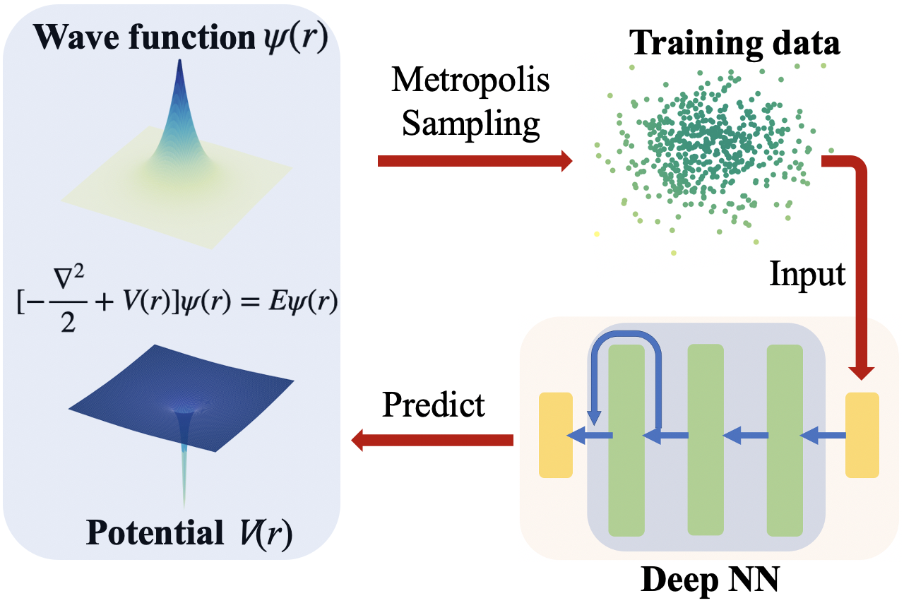
Figure 1: (Color online) The illustration of the main procedures of MPNN. With the potential $U_{\boldsymbol{\theta}}(\mathbf{r})$ predicted by the neural network, the target wave-function $\Psi(\mathbf{r})$ is expected to be the eigenstate of the Hamiltonian $\hat{H}=-\frac{\nabla^{2}}{2}+V(\mathbf{r})$.

II Brief review on quantum potential neural network

Consider the time-independent Schrödinger equation in $D$ dimensions

$$\left[-\frac{\nabla^{2}}{2}+V(\mathbf{r})\right]\Psi(\mathbf{r})=E\Psi(\mathbf{r}),$$ (1)

with the coordinates $\mathbf{r}=(x_{1},\cdots,x_{D})$ and $\frac{\hbar}{m}=1$ as the energy scale. Normally, the task is to solve the eigenstates and energies given the potential $V(\mathbf{r})$. Here, we considered an inverse problem, which is to solve the potential so that the given wave-function $\Psi(\mathbf{r})$ is the eigenstate of the Hamiltonian.

In Ref. [Sehanobish et al., 2021], the authors propose to use a deep neural network named as quantum potential neural network (QPNN) to predict the unknown potential $V(\mathbf{r})$. In detail, the QPNN maps the coordinates to the values of the potential, denoted as $U_{\boldsymbol{\theta}}(\mathbf{r})$ with $\boldsymbol{\theta}$ the variational parameters of the QPNN. With a trial potential, a spatial-dependent energy is introduced as

$$E(\mathbf{r})=-\frac{\nabla^{2}\Psi(\mathbf{r})}{2\Psi(\mathbf{r})}+U_{\boldsymbol{\theta}}(\mathbf{r}).$$ (2)

or

$$E^{\prime}(\mathbf{r})=-\frac{\nabla^{2}|\Psi(\mathbf{r})|}{2|\Psi(\mathbf{r})|}+U_{\boldsymbol{\theta}}(\mathbf{r}).$$ (3)

One can see that $E(\mathbf{r})$ and $E^{\prime}(\mathbf{r})$ is the same if $\Psi(\mathbf{r})$ is real for any $\mathbf{r}$. The authors of Ref. [Sehanobish et al., 2021] proposed to use $E^{\prime}(\mathbf{r})$, considering that the square root of the probability density is much easier to access in experiments.

To characterize the extent of how the Schrödinger equation is satisfied, the loss function is defined as

$$L=\int\left|\nabla E(\mathbf{r})\right|^{2}d\mathbf{r}+\left[U_{\boldsymbol{\theta}}(\mathbf{r}_{0})-V(\mathbf{r}_{0})\right]^{2},$$ (4)

with $\mathbf{r}_{0}$ a given coordinate at which the value of potential $V(\mathbf{r}_{0})$ is previous known. In the practical simulations, one should choose a finite region and discretize the space into pieces with identical width. The loss function is then approximated as

$$L=\sum_{n=1}^{N}\left|\nabla E(\mathbf{r})\right|^{2}_{\mathbf{r}=\mathbf{r}_{n}}+\left[U_{\boldsymbol{\theta}}(\mathbf{r}_{0})-V(\mathbf{r}_{0})\right]^{2},$$ (5)

where $\{\mathbf{r}_{n}\}$ are sampled randomly from the discretized positions.

The loss minimally takes $L=0$. In this case, one has $E(\mathbf{r})=E$ as a constant independent on $\mathbf{r}$, and $U_{\boldsymbol{\theta}}(\mathbf{r}_{0})=V(\mathbf{r}_{0})$. Then $\Psi(\mathbf{r})$ is strictly the eigenstate of the Hamiltonian $\hat{H}_{\boldsymbol{\theta}}=-\frac{\nabla^{2}}{2}+U_{\boldsymbol{\theta}}(\mathbf{r})$, with $U_{\boldsymbol{\theta}}(\mathbf{r}_{0})$ given by the QPNN and $E$ the eigen-energy. With a nonzero loss, one normally has $E$ as a function of the coordinates $\mathbf{r}$, and possibly a deviation between $U_{\boldsymbol{\theta}}(\mathbf{r}_{0})$ and its expected value $V(\mathbf{r}_{0})$. In general, the loss function $L$ in Eq. (5) characterizes how well the potential from the QPNN gives the target wave-function as an eigenstate, and should be minimized. The QPNN can be updated using the gradient decent method as

$$\boldsymbol{\theta}\leftarrow\boldsymbol{\theta}-\eta\frac{\partial L}{\partial\boldsymbol{\theta}},$$ (6)

with $\eta$ the learning rate.

III Metropolis Potential Neural Network Method

The MPNN method is illustrated in Fig. 1. Our goal is solving the potential $V(\mathbf{r})$ while knowing the target wave-function $\Psi(\mathbf{r})$ as the eigenstate of the Hamiltonian. The first step is sampling $N$ positions $\{\mathbf{r}_{n}\}$ according to the probability distribution

$$P(\mathbf{r})=|\Psi(\mathbf{r})|^{2}.$$ (7)

The sampling process can be implemented on a quantum platform if one can make sufficiently many copies of the state $\Psi(\mathbf{r})$, or on a classical computer when $\Psi(\mathbf{r})$ is analytically or numerically accessible. Then a neural network (NN) is applied to predict the values of potential at these positions $\{U_{\boldsymbol{\theta}}(\mathbf{r}_{n})\}$.

To estimate how the potential predicted by the NN satisfies the Schrödinger equation, we define the loss function as mean-square error of the deviations that reads

$$L= \sqrt{\frac{1}{N}\sum_{n=1}^{N}\left|[\hat{H}_{\boldsymbol{\theta}}\Psi(\mathbf{r})]_{\mathbf{r}=\mathbf{r}_{n}}-\tilde{E}\Psi(\mathbf{r}_{n})\right|^{2}}$$ (8)

$$+\lambda\left[U_{\boldsymbol{\theta}}(\mathbf{r}_{0})-V(\mathbf{r}_{0})\right]^{2},$$

Since any global constant shift of the potential (i.e. $V(\mathbf{r})\leftarrow V(\mathbf{r})+\textit{const.}$) would only cause a shift on the energy, a Lagrangian multiplier is added to fix the constant. In other words, we need to know the value of the ground-true potential $V(\mathbf{r}_{0})$ at one certain coordinate $\mathbf{r}_{0}$. The $\lambda$ is a tunable hyper-parameter to control the strength of this constraint. In $\hat{H}_{\boldsymbol{\theta}}=-\frac{\nabla^{2}}{2}+U_{\boldsymbol{\theta}}$, the kinetic energy can be estimated while knowing $\Psi(\mathbf{r})$, and $U_{\boldsymbol{\theta}}$ is given by the NN.

In $L$, we explicitly evaluate the energy $\tilde{E}$ of the target state given $U_{\boldsymbol{\theta}}(\mathbf{r}_{n})$ as

$$\bar{E}=\langle\hat{H}\rangle=\int E(\mathbf{r})P(\mathbf{r})d\mathbf{r}\simeq\frac{1}{N}\sum_{n=1}^{N}E(\mathbf{r}_{n}),$$ (9)

with $E(\mathbf{r}_{n})$ given by Eq. (2) and the positions $\{\mathbf{r}_{n}\}$ sampled from the probability distribution $P(\mathbf{r})$ in Eq. (7). With the loss $L\to 0$, the NN would give a potential $U_{\boldsymbol{\theta}}(\mathbf{r}_{n})\to V(\mathbf{r})$ satisfying the Schrödinger equation (note $V(\mathbf{r})$ denotes the “correct” potential that we expect the NN to give). Meanwhile, the constraint is satisfied, i.e., $|U_{\boldsymbol{\theta}}(\mathbf{r}_{0})-V(\mathbf{r}_{0})|\to 0$, with $L\to 0$.

IV Numerical results

To benchmark the performance of MPNN, we take the ground states of the hydrogen atom and 1D harmonic oscillator (HO) as examples. Note for the hydrogen atom, we do not use the spherical coordinate to transform the Schrödinger equation in three spatial dimensions to a 1D radial equation, just to test the performance on predicting the 3D potentials.

To compare with QPNN, here we use the same architecture of the NN. There are three hidden layers in the NN, where the number of the hidden variables in each layer is no more than 128. A residual channel is added between second and third layers. We use Adam as the optimizer to control the learning rate $\eta$ [see Eq. (6)]. The testing set are sampled independently from the training set. In other words, the coordinates in the testing set are different from those in the training set.

To show the accuracy, we demonstrate in Table 1 (a) the error of potential as

$$\varepsilon=\frac{1}{N}\sum_{n=1}^{N}\left|U_{\boldsymbol{\theta}}(\mathbf{r}_{n})-V(\mathbf{r}_{n})\right|.$$ (10)

We evaluate $\varepsilon$ by averagely taking $20\times 20\times 20=8000$ coordinates $\{\mathbf{r}_{n}\}$ in $x,y,z\in[-1,1]$. Besides QPNN and MPNN, we also test a modified version of QPNN by simply replacing the purely random sampling by Metropolis sampling, which we denote as QPNN+MS. In specific, the coordinates $\{\mathbf{r}_{n}\}$ to evaluate the loss function in Eq. (5) are randomly obtained according to the probability in Eq. (7). Other parts including the NN are the same as the QPNN. For MPNN, we use the loss function given in Eq. (8) where $\{\mathbf{r}_{n}\}$ are also obtained by Metropolis sampling. Our results indicate that one should explicitly involve the energy in the loss function as Eq. (8) to give full play to the advantages of Metropolis sampling. The lowest losses is stably obtained by MPNN for these two systems.

(a) Error of potential $\varepsilon$ QPNN QPNN+MS MPNN hydrogen (ground state) 0.072 0.060 0.028 1D HO (2${}^{\text{nd}}$ excitation) 0.042 0.016 0.006

(b) Energy $\bar{E}$ Exact QPNN QPNN+MS MPNN hydrogen (ground state) -0.5 -0.486 -0.534 -0.493 1D HO (2${}^{\text{nd}}$ excitation) 2.5 2.474 2.519 2.506

Table 1: (a) The error of potential $\varepsilon$ in Eq. (10) and (b) the energy $\bar{E}$ obtained by QPNN, QPNN with Metropolis sampling (MS) as another baseline for comparison, and MPNN. We take the ground state of the hydrogen atom and the second excited state of 1D harmonic oscillator (HO) as examples. The numbers of hidden variables in the three layers of the NN are taken as 32, 128, and 128, respectively, same as those in Ref. [Sehanobish et al., 2021]. See more details about the evaluations of the error and energy for these three methods in the main text.

Table 1 (b) shows the energies by QPNN, QPNN with Metropolis sampling, and MPNN. For QPNN, if $\Psi(\mathbf{r})$ is an eigenstate of $\hat{H}_{\boldsymbol{\theta}}$, one will have a zero loss and $E(\mathbf{r})$ in Eq. (2) as a constant. Therefore, it is a reasonable evaluation of the energy for QPNN using the average of $E(\mathbf{r})$ as

$$\bar{E}_{\text{QPNN}}=\frac{1}{N}\sum_{n=1}^{N}E(\mathbf{r}_{n}).$$ (11)

A more reasonable choice to evaluate the average of the Hamiltonian $\langle\hat{H}_{\boldsymbol{\theta}}\rangle$ for $\Psi(\mathbf{r})$, for which the correct way is to calculate a weighted average as Eq. (9). For this reason, we use Metropolis sampling to get the positions $\{\mathbf{r}_{n}\}$ in QPNN+MS. Another potential advantage of using Metropolis sampling is that the positions with $|\Psi(\mathbf{r})|\to 0$ will be avoided since the probability of having these positions will be vanishing. For the nonzero $\{\mathbf{r}_{n}\}$, we have $E(\mathbf{r}_{n})=E^{\prime}(\mathbf{r}_{n})$.

From our results, we do not see obvious improvement on evaluating the energy by introducing Metropolis sampling to the QPNN. The error compared with the exact solution is around $O(10^{-1})$. One possible reason is that the energy is not explicitly involved in the loss function, i.e., in the optimization. The MPNN method gives the most accurate among these three approaches, with the error around $O(10^{-3})$.

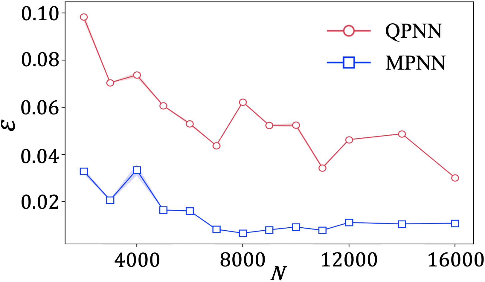
Figure 2: (Color online) The average of the error $\varepsilon$ [Eq. (10)] by MPNN and QPNN with different numbers of samples $N$ used to optimize NN. For each point in the curve, we implement 10 independent simulations to obtain the average and the variance that is $O(10^{-3})$ or less (illustrated by the shadows). The numbers of hidden variables in the three layers of the NN are taken as 128, 128, and 128, respectively.

MPNN also shows its advantage on the sampling efficiency. Fig. 2 demonstrates the average of the error $\varepsilon$ [Eq. (10)] with different numbers of samples $N$ used to optimize NN. We implement 10 independent simulations to calculate the average and variance of $\varepsilon$ for each $N$. Note the fluctuations of $\varepsilon$ are from the randomness in the initialization of the variational parameters in the NN and the sampling processes. The variances are illustrated by the shadows, which are around $O(10^{-3})$ or less. With a same $N$, MPNN achieves a lower error than QPNN.

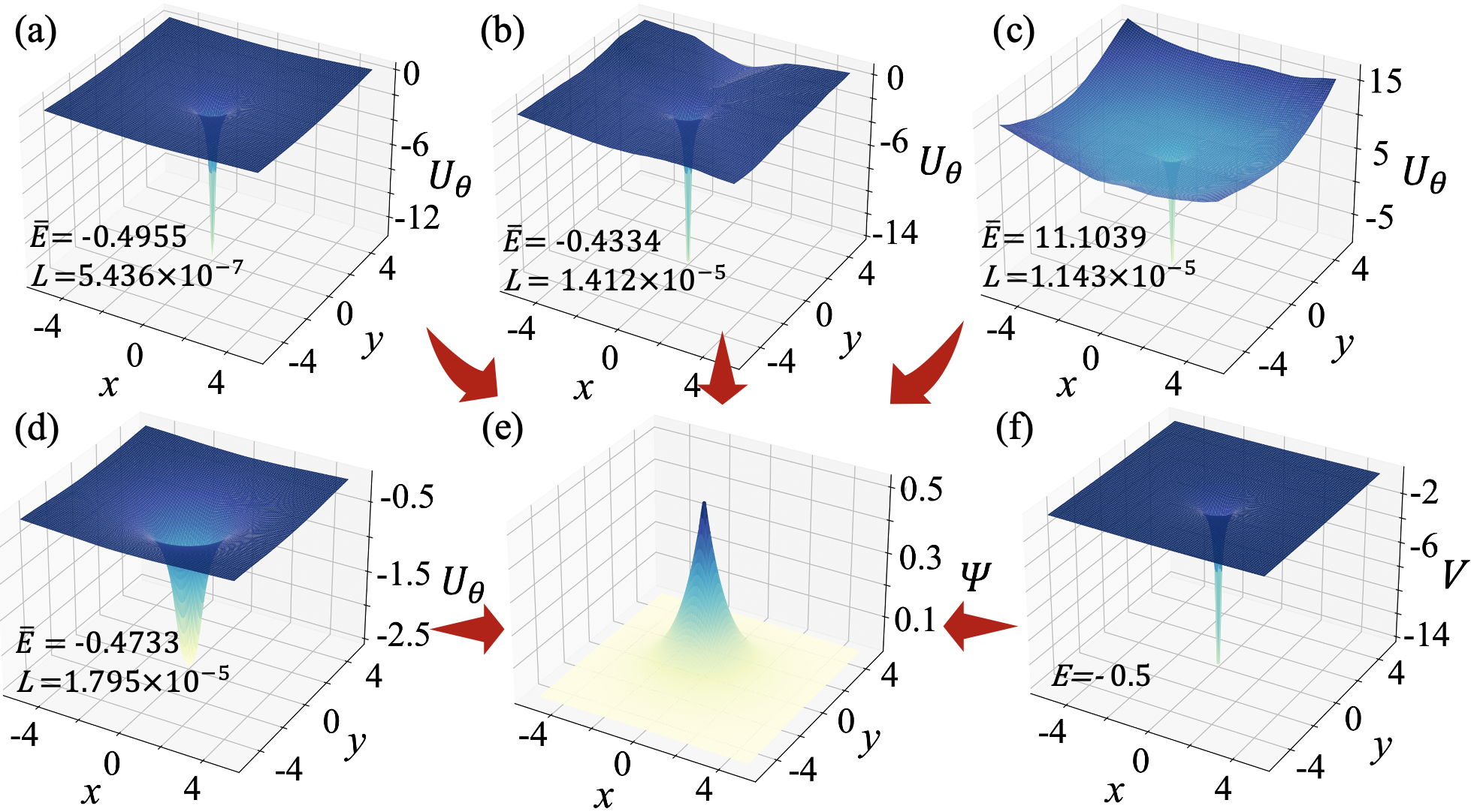
Figure 3: (Color online) (a)-(d) show four different potentials $U_{\boldsymbol{\theta}}(\mathbf{r})$ that approximately give the ground-state wave-function $\Psi(\mathbf{r})$ of the hydrogen atom with the losses $L\simeq O(10^{-5})-O(10^{-6})$. The potential in (a) is obtained by our MPNN, which gives the lowest loss and the best estimation near the singular point $\mathbf{r}=0$. The numbers of hidden variables are taken as the same values as those in Fig. 2. See more details of (a)-(d) in the main text. We show in (e) the target wave-function $\Psi(\mathbf{r})$, and in (f) the exact potential $V(\mathbf{r})=-\frac{1}{|\mathbf{r}|}$. In all sub-figures, we fix $z=0$ to illustrate the $x$- and $y$-dependence of the potentials or wave-function.

There exist many local minimums of the loss function. A bad local minimum might give rise to an incorrect or inaccurate energy, even if the value of the loss is small. Figs. 3 (a)-(d) show four different $U_{\boldsymbol{\theta}}$ that give the losses $L\sim O(10^{-5})-O(10^{-6})$ for the ground state of the hydrogen atom. Figs. 3 (e) and (f) show the exact ground-state wave-function $\Psi(\mathbf{r})$ and the potential $V(\mathbf{r})=-\frac{1}{|\mathbf{r}|}$. We fix $z=0$ to illustrate the $x-y$ dependence of the potentials or wave-function.

Compared with the expected potential $V(\mathbf{r})$, the best result is obtained by the MPNN, illustrated in Fig. 3 (a). By changing the initialization strategy of the NN, say without multiplying the initial $\boldsymbol{\theta}$ with $\delta$, one may obtain a different energy with a similar loss, as shown in Fig. 3 (b). Our simulation results indicate an effective initialization strategy by letting the initial potential be near the hyper-surface of $V=0$. This can be done by first randomly initializing all $\boldsymbol{\theta}$ in the NN and then multiplying them with a small factor, e.g., $\delta=0.01$.

In Fig. 3 (c), we set $\lambda=0$, then an extra degree of freedom will appear. It can be easily seen that a potential $V^{\prime}(\mathbf{r})=V(\mathbf{r})+C$ will be the solution of our inverse problem for any constant $C$ if $V(\mathbf{r})$ is the solution. The penalty term $\lambda\left[U_{\boldsymbol{\theta}}(\mathbf{r}_{0})-V(\mathbf{r}_{0})\right]^{2}$ is to fix this degrees of freedom to give the correct energy.

Fig. 3 (d) shows the $U_{\boldsymbol{\theta}}$ obtained by the QPNN. The dominant error is the data that are taken near the center of the potential. For the MPNN, the positions with larger $|\Psi(\mathbf{r})|$ are taken more frequently in the Metropolis sampling. Better prediction is obtained since such data contribute more to the physical properties, such as the observables and the gradients in optimizing the NN, compared with those that have small $|\Psi(\mathbf{r})|$.

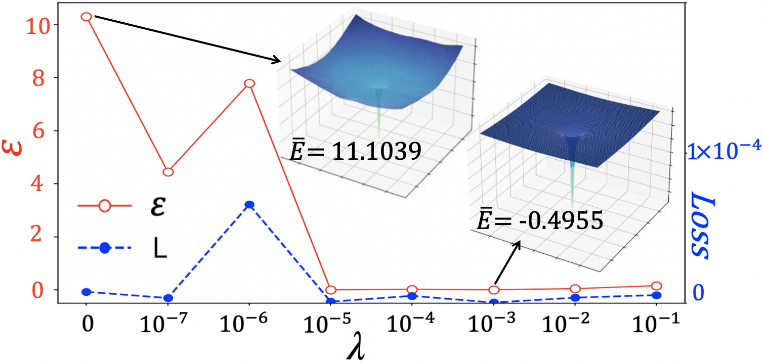
Figure 4: (Color online) The error of the potential [Eq. (10)] and the loss [Eq. (8)] with different values of the Lagrangian multiplier $\lambda$. The insets show two examples of the predicted potential with $z=0$. We take the numbers of hidden variables to be the same values as those in Fig. 2.

The penalty term $\lambda\left[U_{\boldsymbol{\theta}}(\mathbf{r}_{0})-V(\mathbf{r}_{0})\right]^{2}$ is to fix the degrees of freedom with a global shift of the potential. The coefficient determines how strictly we require the NN to give the correct value at the position $\mathbf{r}_{0}$. Fig. 4 shows the error $\varepsilon$ in Eq. (10) of the hydrogen atom with different values of $\lambda$. For $\lambda=0$, meaning we do not require $U_{\boldsymbol{\theta}}(\mathbf{r}_{0})=V(\mathbf{r}_{0})$, the predicted potential can be shifted determined by the initial values of $\boldsymbol{\theta}$. Thus one cannot correctly give the energy $\bar{E}$, and the error $\varepsilon$ is significant. But the loss is small with $L\sim O(10^{-4})$. This means without knowing the potential at some position, we cannot uniquely give the eigen-energy of $\Psi$ but can still give the potential $U_{\boldsymbol{\theta}}$ so that $\Psi$ is the eigenstate of $\hat{H}_{\boldsymbol{\theta}}$.

As $\lambda$ increases to certain extent, we are able to obtain the expected potential $V(\mathbf{r})$ with small $\varepsilon$. Note the loss is still small, which fluctuates around $L\sim O(10^{-4})-O(10^{-5})$. In such cases, we obtain accurate predictions of the eigen-energy $\bar{E}\simeq-0.5$.

V Summary

The hybridization of machine learning with quantum physics brings new possibility to solve the important problems that are challenging using the conventional approaches. Stimulated by the quantum potential neural network, we consider to predict the potential in Schrödinger equation, with which the target state $\Psi$ is the eigenstate of the Hamiltonian. The Metropolis potential neural network (MPNN) is proposed to predict the potential by combining deep neural network and Metropolis sampling. With the benchmark on the harmonic oscillator and hydrogen atom, MPNN exhibits excellent precision and stability on both predicting the potential and evaluating the eigen-energy. Our proposal can be readily generalized to inversely solving the Schrödinger equation of multiple electrons, and the differentiation equations for other physical problems.

References

- Carleo et al. (2019) Giuseppe Carleo, Ignacio Cirac, Kyle Cranmer, Laurent Daudet, Maria Schuld, Naftali Tishby, Leslie Vogt-Maranto, and Lenka Zdeborová, “Machine learning and the physical sciences,” Reviews of Modern Physics 91, 045002 (2019).
- Ramprasad et al. (2017) Rampi Ramprasad, Rohit Batra, Ghanshyam Pilania, Arun Mannodi-Kanakkithodi, and Chiho Kim, “Machine learning in materials informatics: recent applications and prospects,” npj Computational Materials 3, 54 (2017).
- Butler et al. (2018) Keith T. Butler, Daniel W. Davies, Hugh Cartwright, Olexandr Isayev, and Aron Walsh, “Machine learning for molecular and materials science,” Nature 559, 547–555 (2018).
- Xie and Grossman (2018) Tian Xie and Jeffrey C. Grossman, “Crystal Graph Convolutional Neural Networks for an Accurate and Interpretable Prediction of Material Properties,” Physical Review Letters 120, 145301 (2018).
- Gubernatis and Lookman (2018) J. E. Gubernatis and T. Lookman, “Machine learning in materials design and discovery: Examples from the present and suggestions for the future,” Phys. Rev. Materials 2 (2018), 10.1103/PhysRevMaterials.2.120301.
- Doan et al. (2020) Hieu A. Doan, Garvit Agarwal, Hai Qian, Michael J. Counihan, Joaquín Rodríguez-López, Jeffrey S. Moore, and Rajeev S. Assary, “Quantum Chemistry-Informed Active Learning to Accelerate the Design and Discovery of Sustainable Energy Storage Materials,” Chemistry of Materials 32, 6338–6346 (2020).
- Ma et al. (2021) Xing-Yu Ma, Hou-Yi Lyu, Xue-Juan Dong, Zhen Zhang, Kuan-Rong Hao, Qing-Bo Yan, and Gang Su, “Voting Data-Driven Regression Learning for Accelerating Discovery of Advanced Functional Materials and Applications to Two-Dimensional Ferroelectric Materials,” The Journal of Physical Chemistry Letters 12, 973–981 (2021).
- Han et al. (2019) Jiequn Han, Linfeng Zhang, and Weinan E, “Solving many-electron Schrödinger equation using deep neural networks,” Journal of Computational Physics 399, 108929 (2019).
- Schütt et al. (2019) K. T. Schütt, M. Gastegger, A. Tkatchenko, K.-R. Müller, and R. J. Maurer, “Unifying machine learning and quantum chemistry with a deep neural network for molecular wavefunctions,” Nature Communications 10, 5024 (2019).
- Pfau et al. (2020) David Pfau, James S. Spencer, Alexander G. D. G. Matthews, and W. M. C. Foulkes, “Ab initio solution of the many-electron Schrödinger equation with deep neural networks,” Physical Review Research 2, 033429 (2020).
- Manzhos (2020) Sergei Manzhos, “Machine learning for the solution of the Schrödinger equation,” Machine Learning: Science and Technology 1, 013002 (2020).
- Hermann et al. (2020) Jan Hermann, Zeno Schätzle, and Frank Noé, “Deep-neural-network solution of the electronic Schrödinger equation,” Nature Chemistry 12, 891–897 (2020).
- Ryczko et al. (2019) Kevin Ryczko, David Strubbe, and Isaac Tamblyn, “Deep Learning and Density Functional Theory,” Physical Review A 100, 022512 (2019).
- Denner et al. (2020) M. Michael Denner, Mark H. Fischer, and Titus Neupert, “Efficient Learning of a One-dimensional Density Functional Theory,” Physical Review Research 2, 033388 (2020).
- Carleo and Troyer (2017) Giuseppe Carleo and Matthias Troyer, “Solving the quantum many-body problem with artificial neural networks,” Science 355, 602–606 (2017).
- Glasser et al. (2018) Ivan Glasser, Nicola Pancotti, Moritz August, Ivan D. Rodriguez, and J. Ignacio Cirac, “Neural-Network Quantum States, String-Bond States, and Chiral Topological States,” Physical Review X 8 (2018), 10.1103/PhysRevX.8.011006.
- Jensen and Wasserman (2018) Daniel S. Jensen and Adam Wasserman, “Numerical methods for the inverse problem of density functional theory,” International Journal of Quantum Chemistry 118, e25425 (2018).
- Zhang et al. (2019) Yi Zhang, A. Mesaros, K. Fujita, S. D. Edkins, M. H. Hamidian, K. Ch’ng, H. Eisaki, S. Uchida, J. C. Séamus Davis, Ehsan Khatami, and Eun-Ah Kim, “Machine learning in electronic-quantum-matter imaging experiments,” Nature 570, 484–490 (2019).
- Fournier et al. (2020) Romain Fournier, Lei Wang, Oleg V. Yazyev, and QuanSheng Wu, “Artificial neural network approach to the analytic continuation problem,” Phys. Rev. Lett. 124, 056401 (2020).
- Teoh et al. (2020) Yi Hong Teoh, Marina Drygala, Roger G Melko, and Rajibul Islam, “Machine learning design of a trapped-ion quantum spin simulator,” Quantum Science and Technology 5, 024001 (2020).
- Behler and Parrinello (2007) Jörg Behler and Michele Parrinello, “Generalized Neural-Network Representation of High-Dimensional Potential-Energy Surfaces,” Physical Review Letters 98, 146401 (2007).
- Schütt et al. (2014) K. T. Schütt, H. Glawe, F. Brockherde, A. Sanna, K. R. Müller, and E. K. U. Gross, “How to represent crystal structures for machine learning: Towards fast prediction of electronic properties,” Physical Review B 89, 205118 (2014).
- Jiang et al. (2016) Bin Jiang, Jun Li, and Hua Guo, “Potential energy surfaces from high fidelity fitting of ab initio points: the permutation invariant polynomial - neural network approach,” International Reviews in Physical Chemistry 35, 479–506 (2016).
- Hegde and Bowen (2017) Ganesh Hegde and R. Chris Bowen, “Machine-learned approximations to Density Functional Theory Hamiltonians,” Scientific Reports 7, 42669 (2017).
- Berthusen et al. (2021) Noah F. Berthusen, Yuriy Sizyuk, Mathias S. Scheurer, and Peter P. Orth, “Learning crystal field parameters using convolutional neural networks,” SciPost Phys. 11, 11 (2021).
- Kokail et al. (2021) Christian Kokail, Bhuvanesh Sundar, Torsten V. Zache, Andreas Elben, Benoît Vermersch, Marcello Dalmonte, Rick van Bijnen, and Peter Zoller, “Quantum Variational Learning of the Entanglement Hamiltonian,” arXiv:2105.04317 [cond-mat, physics:quant-ph] (2021).
- Xin et al. (2019) Tao Xin, Sirui Lu, Ningping Cao, Galit Anikeeva, Dawei Lu, Jun Li, Guilu Long, and Bei Zeng, “Local-measurement-based quantum state tomography via neural networks,” npj Quantum Information 5, 109 (2019).
- Wang et al. (2015) Sheng-Tao Wang, Dong-Ling Deng, and L-M Duan, “Hamiltonian tomography for quantum many-body systems with arbitrary couplings,” New Journal of Physics 17, 093017 (2015).
- Bairey et al. (2019) Eyal Bairey, Itai Arad, and Netanel H. Lindner, “Learning a local hamiltonian from local measurements,” Phys. Rev. Lett. 122, 020504 (2019).
- Ma et al. (2020) Xinran Ma, Z C Tu, and Shi-Ju Ran, “Deep learning quantum states for hamiltonian predictions,” arXiv:2012.03019v1 (2020).
- Sehanobish et al. (2021) Arijit Sehanobish, Hector H. Corzo, Onur Kara, and David van Dijk, “Learning Potentials of Quantum Systems using Deep Neural Networks,” arXiv:2006.13297 (2021).
- (32) Nicholas Metropolis, Arianna W Rosenbluth, Marshall N Rosenbluth, Augusta H Teller, and Edward Teller, “Equation of State Calculations by Fast Computing Machines,” .
- Inack et al. (2018) E. M. Inack, G. E. Santoro, L. Dell’Anna, and S. Pilati, “Projective quantum monte carlo simulations guided by unrestricted neural network states,” Phys. Rev. B 98, 235145 (2018).
- Nagy and Savona (2019) Alexandra Nagy and Vincenzo Savona, “Variational quantum monte carlo method with a neural-network ansatz for open quantum systems,” Phys. Rev. Lett. 122, 250501 (2019).
- Choo et al. (2019) Kenny Choo, Titus Neupert, and Giuseppe Carleo, “Two-dimensional frustrated model studied with neural network quantum states,” Phys. Rev. B 100, 125124 (2019).
- Casares et al. (2021) P. A. M. Casares, Roberto Campos, and M. A. Martin-Delgado, “QFold: Quantum Walks and Deep Learning to Solve Protein Folding,” arXiv:2101.10279 (2021).
- Berg (2004) B. A. Berg, Markov Chain Monte Carlo Simulations and Their Statistical Analysis (World Scientific, Singapore, 2004).
- Landau and Binder (2009) D. P. Landau and K. Binder, A Guide to Monte Carlo Simulations in Statistical Physics (Cambridge University Press,Cambridge, UK, 2009).
- Foulkes et al. (2001) W. M. C. Foulkes, L. Mitas, R. J. Needs, and G. Rajagopal, “Quantum Monte Carlo simulations of solids,” Reviews of Modern Physics 73, 33–83 (2001).
- Goodfellow and Courville (2016) Y. Bengio Goodfellow, I. and A. Courville, Deep Learning (MIT Press, Cambridge, MA, 2016).