Optimal error estimation of a time-spectral method for fractional diffusion problems with low regularity data

Abstract

This paper is devoted to the error analysis of a time-spectral algorithm for fractional diffusion problems of order $\alpha$ ($0<\alpha<1$). The solution regularity in the Sobolev space is revisited, and new regularity results in the Besov space are established. A time-spectral algorithm is developed which adopts a standard spectral method and a conforming linear finite element method for temporal and spatial discretizations, respectively. Optimal error estimates are derived with nonsmooth data. Particularly, a sharp temporal convergence rate $1+2\alpha$ is shown theoretically and numerically.

Keywords: fractional diffusion problem, finite element, spectral method, Jacobi polynomial, low regularity, Besov space, optimal error estimate.

1 Introduction

This paper considers the following time fractional diffusion problem:

$$\left\{\begin{aligned} \operatorname{D}_{0+}^{\alpha}(u-u_{0})-\Delta u&=f&&\text{in~{}$\Omega\times(0,T)$,}\\ u&=0&&\text{on $\partial\Omega\times(0,T)$,}\\ u(0)&=u_{0}&&\text{in $\Omega$,}\end{aligned}\right.$$ (1)

where $T>0,\,0<\alpha<1$, $\operatorname{D}_{0+}^{\alpha}$ is a Riemann–Liouville fractional differential operator (see Section 2), $\Omega\subset\mathbb{R}^{d}$ ($d=1,2,3$) is a convex polygonal domain, and $u_{0}$ and $f$ are given data.

Problem 1 is widely used in modeling of anomalous diffusion process [45, 46] and anomalous transport [38, 63], for its capability of accurately describing models with non-locality and historical memory [23, 52]. For theoretical study to the problem, e.g. the weak solution and its regularity, we refer to [15, 33, 35, 54].

Many numerical methods have been developed in the past a dozen years. Among existing works, four types of temporal discretization are most prevailing, i.e., finite difference methods (L-type schemes) [2, 24, 36, 41], convolution quadrature methods [11, 13, 60, 62], finite element methods [27, 28, 29, 31] and spectral methods [26, 35, 55, 64]. Under certain circumstances, problem 1 has an equivalent form like

$$\left\{\begin{aligned} u_{t}-\operatorname{D}_{0+}^{1-\alpha}\Delta u&=g&&\text{in~{}$\Omega\times(0,T)$,}\\ u&=0&&\text{on $\partial\Omega\times(0,T)$,}\\ u(0)&=u_{0}&&\text{in $\Omega$,}\end{aligned}\right.$$ (2)

where $g=\operatorname{D}_{0+}^{1-\alpha}f$. In the literature, both 1 and 2 are called time fractional diffusion equations or time fractional subdiffusion equations. For the solution regularity and numerical analysis of problem 2, especially in the case of nonsmooth data, we refer the reader to [25, 42, 43, 48, 50, 51].

It is well-known that the solution to problem 1 generally has boundary singularity (near $0+$) in temporal direction. If $f=0$ and $u_{0}\neq 0$, or $u_{0}=0$ and $f$ is smooth, then one can obtain growth estimates of the solution [19, 20] or even find out the leading singular term $ct^{\alpha}$ of the solution [33]. Due to the singularity, the accuracy order $2-\alpha$ of the L1 scheme [36] deteriorates into 1 in the case of $f=0$ and $u_{0}\neq 0$, whether the initial data $u_{0}$ is smooth or not [21]. In the same situation, a piecewise constant discontinuous Galerkin (DG) semidiscretization was analyzed in [44]. The error estimate results of [21, 44] can be summarized as follows: for any temporal grid node $t_{j}=j\tau$ with $j=1,2,\cdots,J$ and $\tau=T/J$,

$$\left\lVert{(u-U)(t_{j})}\right\rVert_{L^{2}(\Omega)}\leqslant C\left\{\begin{aligned} &t_{j}^{\alpha-1}\tau\left\lVert{u_{0}}\right\rVert_{\dot{H}^{2}(\Omega)},&&\text{for L1 in }\cite[cite]{[\@@bibref{}{jin_analysis_2015}{}{}]}\\ &t_{j}^{-1}\tau\left\lVert{u_{0}}\right\rVert_{L^{2}(\Omega)},&&\text{for L1 in }\cite[cite]{[\@@bibref{}{jin_analysis_2015}{}{}]}\text{ and }\text{DG in }\cite[cite]{[\@@bibref{}{McLean2015Time}{}{}]}.\end{aligned}\right.$$ (3)

Hence, if $u_{0}\in L^{2}(\Omega)$, then the first order accuracy under $L^{\infty}(0,T;L^{2}(\Omega))$-norm is only achieved far away from the origin, and the global convergence rate degenerates as $t_{j}$ approaches to zero; and if $u_{0}\in\dot{H}^{2}(\Omega)$, then the global rate reduces to $\tau^{\alpha}$. The estimates in 3 coincide with the solution regularity in Sobolev space (see Theorem 3.2):

$$\left\{\begin{aligned} {}&\epsilon^{3/2}\left\lvert{u}\right\rvert_{H^{1/2-\epsilon}(0,T;L^{2}(\Omega))}\leqslant{}C_{\alpha,T}\left\lVert{u_{0}}\right\rVert_{L^{2}(\Omega)},&&0<\epsilon\leqslant 1/2,\\ {}&\sqrt{2\gamma-\gamma^{2}}\left\lVert{u}\right\rVert_{H^{(1+\alpha\gamma)/2}(0,T;L^{2}(\Omega))}\leqslant{}C_{\alpha,T,\Omega}\left\lVert{u_{0}}\right\rVert_{\dot{H}^{\gamma}(\Omega)},&&0<\gamma<2,\end{aligned}\right.$$

which means that $u_{0}\in L^{2}(\Omega)\nRightarrow u\in L^{\infty}(0,T;L^{2}(\Omega))$ and that

$$u_{0}\in\dot{H}^{2}(\Omega)\Rightarrow u\in H^{(1+\alpha\gamma)/2}(0,T;L^{2}(\Omega))\hookrightarrow L^{\infty}(0,T;L^{2}(\Omega)),$$

since $\gamma\in(0,2)$ implies the embedding relation above.

To improve the temporal accuracy, graded meshes were used in [24, 49, 58] and some correction techniques were proposed in [12, 22, 30, 61]. However, most of the existing works using graded meshes require some assumption of growth estimate on the true solution, and the analyses of correction schemes for 3 are mainly based on the Laplace transform, which is only applicable for uniform temporal grids, and the obtained convergence rates have the form $t_{j}^{-q}\tau^{p}$ with $0<q\leqslant p$ (like (3)), which deteriorate near the origin. In [32], several technical stability results were developed to establish the optimal first order accuracy of a piecewise constant DG method on graded meshes. Spectral methods with singular basis functions were presented [7, 55], but so far no rigorous convergence analysis is available with low regularity data. In [8], a multi-domain Petrov–Galerkin spectral method with a singular basis and geometrically graded meshes was proposed, and the exponential decay was verified numerically with nonsmooth initial data.

In the 1980s, Gui and Babuška [17] established the optimal approximation of order $1+2\beta$ under the $L^{2}$-norm of the Legendre orthogonal expansion for the singular function $(x+1)^{\beta}$ on $(-1,1)$. Later Babuška and Suri [4] extended this result to a $p$-version finite element method for solving two dimensional elliptic equations, and proved the sharp accuracy of order $2\beta$ under an energy norm, by assuming that the solution has the explicit singular expression $r^{\beta}$ around the origin.

Note that the singular functions mentioned above have boundary singularities as well but the achieved convergence rates agree with their regularity in the Besov space. In view of the boundary singularity of the solution to problem 1, one may wonder whether this happens to the convergence behavior of a time-spectral method. For simplicity, let us start with a fractional ordinary differential equation

$$\operatorname{D}_{0+}^{\alpha}(y-y_{0})+\lambda y=0\quad\text{in}\quad(0,T),$$ (4)

where $y_{0}\in\,{\mathbb{R}}$ and $\lambda>0$. Invoking the Laplace transform gives the solution expression

$$y(t)=y_{0}\sum_{k=0}^{\infty}\frac{(-\lambda t^{\alpha})^{k}}{\Gamma(\alpha k+1)},\quad 0\leqslant t\leqslant T.$$ (5)

Note that for a given fixed (small) $\lambda>0$, we have $y\in H^{1/2+\alpha-\epsilon}(0,T)$ for any $\epsilon>0$ (see 3.1). We adopt a standard Legendre spectral method with polynomial degree $M\in\mathbb{N}$ to seek an approximation $Y_{M}$, and use $Y_{50}$ as a reference solution. Fig. 1 plots the convergence order $1+2\alpha$ under $L^{2}$-norm in the case that $\lambda=y_{0}=T=1$. This agrees with the Besov regularity, ${\mathbb{B}}_{-\alpha,0}^{1+2\alpha-\epsilon}(0,T)$ for any $\epsilon>0$, of 5; see Lemma 3.5. However, if $\lambda$ is extremely large or goes to infinity, then we can see from Lemma 4.1 that the convergence rate will be ruined (we also refer the reader to [8, Section 1.2] for detailed numerical investigations in this case).

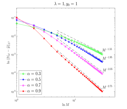
Figure 1: Discretization errors of problem 4 with $\lambda=y_{0}=T=1$. The predicted accuracy is $M^{-1-2\alpha}$.

As for the model problem 1 itself, although there exists a space-time spectral method proposed in [35], to our best knowledge, no such convergence rate $1+2\alpha$ has been mentioned numerically and established rigorously. In fact, it is nontrivial to obtain this result, since now the impact of large $\lambda$ comes from the negative Laplacian operator $-\Delta$ (or its discrete version $-\Delta_{h}$). This motivates us to revisit the convergence analysis of the time-spectral method for time fractional diffusion problem 1. Is it possible to prove the optimal approximation order in terms of Besov regularity with nonsmooth data? Especially, whether the accuracy $1+2\alpha$ can be established or improved?

In this work, we give positive answers to these questions mentioned above. Optimal error estimates with respect to the solution regularity in Besov space are established with low regularity data. Moreover, temporal convergence rates $1+\alpha$ and $1+2\alpha$ under $H^{\alpha/2}(0,T;L^{2}(\Omega))$-norm and $L^{2}(0,T;\dot{H}^{1}(\Omega))$-norm are derived, respectively, which are sharp and cannot be improved even for smoother data.

The rest of this paper is organized as follows. Section 2 introduces some notations, including standard conventions, functional spaces and fractional calculus operators. Section 3 defines the weak solution and establishes its regularity results in Sobolev space and Besov space. Section 4 presents our main error estimates for the time-spectral method, and Section 5 shows several numerical experiments. Finally, Section 6 gives some concluding remarks.

2 Preliminary

For ease of notation, we make some standard conventions. For a Lebesgue measurable subset $\omega$ of $\mathbb{R}^{l}$ ($l=1,2,3$), we use $H^{\gamma}(\omega)$ ($\gamma\in\,{\mathbb{R}}$) and $H_{0}^{\gamma}(\omega)$ ($\gamma>0$) to denote two standard Sobolev spaces [59]. Given $1\leqslant p<\infty$, if $\omega$ is an interval and $\mu$ is a nonnegative measurable function on $\omega$, then $L_{\mu}^{p}(\omega)$ denotes the weighted $L^{p}$-space, and the symbol $\left\langle{a,b}\right\rangle_{\mu}$ means $\int_{\omega}ab\mu$ whenever $ab\in L^{1}_{\mu}(\omega)$; if $\omega$ is a Lebesgue measurable set of $\mathbb{R}^{l}(l=1,2,3,4)$, then $\left\langle{a,b}\right\rangle_{\omega}$ stands for $\int_{\omega}ab$ whenever $ab\in L^{1}(\omega)$; if $X$ is a Banach space, then $\left\langle{\cdot,\cdot}\right\rangle_{X}$ means the duality pairing between $X^{*}$ (the dual space of $X$) and $X$. In particular, if $X$ is a Hilbert space, then $(\cdot,\cdot)_{X}$ means its inner product. If $X$ and $Y$ are two Banach spaces, then $[X,Y]_{\theta,2}$ is the interpolation space constructed by the well-known $K$-method [5]. For $k\in\mathbb{N}$ and any $d$-polytope $\omega\subset\,{\mathbb{R}}^{d}(d=1,2,3)$, $P_{k}(\omega)$ denotes the set of all polynomials defined on $\omega$ with degree no more than $k$.

It is well-known (cf. [10]) that $L^{2}(\Omega)$ has an orthonormal basis $\{\phi_{n}\}_{n=0}^{\infty}$ such that

$$\left\{\begin{aligned} -\Delta\phi_{n}={}&\lambda_{n}\phi_{n},&&\text{in~{}}\Omega,\\ \phi_{n}={}&0,&&\text{on~{}}\partial\Omega,\end{aligned}\right.$$

where $\{\lambda_{n}\}_{n=0}^{\infty}$ is a nondecreasing real positive sequence and $\lambda_{0}=\left\lVert{\nabla\phi_{0}}\right\rVert^{2}_{L^{2}(\Omega)}>0$ depends only on $\Omega$. For any $\gamma\in\,{\mathbb{R}}$, define

$$\dot{H}^{\gamma}(\Omega):=\left\{\sum_{n=0}^{\infty}c_{n}\phi_{n}:\ \sum_{n=0}^{\infty}\lambda_{n}^{\gamma}c_{n}^{2}<\infty\right\}$$

and equip this space with the inner product

$$\left(\sum_{n=0}^{\infty}c_{n}\phi_{n},\sum_{n=0}^{\infty}d_{n}\phi_{n}\right)_{\dot{H}^{\gamma}(\Omega)}:=\sum_{n=0}^{\infty}\lambda_{n}^{\gamma}c_{n}d_{n},\quad\text{for all }\sum_{n=0}^{\infty}c_{n}\phi_{n},\sum_{n=0}^{\infty}d_{n}\phi_{n}\in\dot{H}^{\gamma}(\Omega).$$

The induced norm is denoted by $\left\lVert{\cdot}\right\rVert_{\dot{H}^{\gamma}(\Omega)}=\sqrt{\left({\cdot,\cdot}\right)_{\dot{H}^{\gamma}(\Omega)}}$. Note that $\dot{H}^{\gamma}(\Omega)$ is a Hilbert space and has an orthonormal basis $\{\lambda_{n}^{-\gamma/2}\phi_{n}\}_{n=0}^{\infty}$.

Given any $0<\gamma<2$, we introduce the space

$${}_{0}H^{\gamma}(0,T):=[L^{2}(0,T),{}_{0}H^{2}(0,T)]_{\gamma/2,2},$$

where ${}_{0}H^{2}(0,T):=\left\{v\in H^{2}(0,T):v(0)=v^{\prime}(0)=0\right\}$ with norm $\left\lVert{v}\right\rVert_{{}_{0}H^{2}(0,T)}:=\left\lVert{v^{\prime\prime}}\right\rVert_{L^{2}(0,T)}$. Therefore, using the interpolation theorem of bounded linear operators [39, Theorem 1.6] yields

$$\left\lVert{v}\right\rVert_{[L^{2}(0,T),H^{2}(0,T)]_{\gamma/2,2}}\leqslant\left\lVert{v}\right\rVert_{{}_{0}H^{\gamma}(0,T)}\quad\forall\,v\in{}_{0}H^{\gamma}(0,T).$$ (6)

In addition, if $0<\gamma<1/2$, then by [37, Chapter 1], the relation ${}_{0}H^{\gamma}(0,T)=H^{\gamma}(0,T)$ holds in the sense of equivalent norms, and in this case (i.e., $0<\gamma<1/2$) we have an alternative norm, which is defined by

$$\left\lvert{w}\right\rvert_{H^{\gamma}(0,T)}:=\left(\int_{\mathbb{R}}\left\lvert{\xi}\right\rvert^{2\gamma}\left\lvert{\mathcal{F}(w\chi_{(0,T)})(\xi)}\right\rvert^{2}\,\mathrm{d}\xi\right)^{1/2}\quad\forall w\in H^{\gamma}(0,T),$$

where $\mathcal{F}:L^{2}(\mathbb{R})\to L^{2}(\mathbb{R})$ is the Fourier transform and $\chi_{(0,T)}$ is the indicator function of $(0,T)$.

Let $X$ be a separable Hilbert space with an inner product $(\cdot,\cdot)_{X}$ and an orthonormal basis $\{e_{n}:n\in\mathbb{N}\}$. For any $\gamma\in\,{\mathbb{R}}$, let $H^{\gamma}(0,T;X)$ be a usual vector-valued Sobolev space defined by

$$H^{\gamma}(0,T;X):=\left\{\sum_{n=0}^{\infty}v_{n}e_{n}:\,\sum_{n=0}^{\infty}\left\lVert{v_{n}}\right\rVert_{H^{\gamma}(0,T)}^{2}<\infty\right\},$$ (7)

with the norm

$$\left\lVert{v}\right\rVert_{H^{\gamma}(0,T;X)}:=\left(\sum_{n=0}^{\infty}\left\lVert{(v,e_{n})_{X}}\right\rVert_{H^{\gamma}(0,T)}^{2}\right)^{1/2}\quad\forall\,v\in H^{\gamma}(0,T;X).$$

The space ${}_{0}H^{\gamma}(0,T;X)$ for $0<\gamma<2$ is defined in a similar way as 7.

For $a,b>-1$, let $\{S_{k}^{a,b}\}_{k=0}^{\infty}$ be the family of shifted Jacobi polynomials on $(0,T)$ with respect to the weight $\mu^{a,b}(t)=(T-t)^{a}t^{b}$; see Appendix A. Given $\gamma\geqslant 0$, we introduce the Besov space (also known as the weighted Sobolev space, cf. [3]) defined by

$${\mathbb{B}}_{a,b}^{\gamma}(0,T):=\left\{\sum_{k=0}^{\infty}v_{k}S_{k}^{a,b}:\,\sum_{k=0}^{\infty}(1+k^{2\gamma})\xi_{k}^{a,b}v_{k}^{2}<\infty\right\},$$ (8)

where $\xi_{k}^{a,b}$ is given by 65, and endow this space with the norm

$$\left\lVert{v}\right\rVert_{{\mathbb{B}}_{a,b}^{\gamma}(0,T)}:=\left(\sum_{k=0}^{\infty}(1+k^{2\gamma})\xi_{k}^{a,b}v_{k}^{2}\right)^{1/2}\quad\forall\,v=\sum_{k=0}^{\infty}v_{k}S_{k}^{a,b}\in{\mathbb{B}}_{a,b}^{\gamma}(0,T).$$

In addition, for any separable Hilbert space $X$, the vector-valued space ${\mathbb{B}}_{a,b}^{\gamma}(0,T;X)$ can be defined in a similar way as that of 7.

To the end, let us introduce the Riemann–Liouville fractional calculus operators and list some important lemmas. For any $\gamma>0$ and $v\in L^{1}(0,T;X)$, define the fractional integrals of order $\gamma$ as follows:

$$\left(\operatorname{D}_{0+}^{-\gamma}v\right)(t) :=\frac{1}{\Gamma(\gamma)}\int_{0}^{t}(t-s)^{\gamma-1}v(s)\,\mathrm{d}s,\quad t\in(0,T),$$

$$\left(\operatorname{D}_{T-}^{-\gamma}v\right)(t) :=\frac{1}{\Gamma(\gamma)}\int_{t}^{T}(s-t)^{\gamma-1}v(s)\,\mathrm{d}s,\quad t\in(0,T),$$

where $\Gamma(\cdot)$ denotes the Gamma function

$$\Gamma(z):=\int_{0}^{\infty}t^{z-1}e^{-t}\,{\rm d}t,\quad z>0.$$ (9)

For $k<\gamma<k+1$ with $k\in\mathbb{N}$, define the left-sided and right-sided Riemann–Liouville fractional derivative operators of order $\gamma$ respectively by

$$\operatorname{D}_{0+}^{\gamma}:={}\operatorname{D}^{k}\operatorname{D}_{0+}^{\gamma-k},\quad\operatorname{D}_{T-}^{\gamma}:={}(-\operatorname{D})^{k}\operatorname{D}_{T-}^{\gamma-k},$$

where $\operatorname{D}$ is the first-order generalized derivative operator.

Lemma 2.1 ([9]).

If $-1/2<\gamma<1/2$ and $v,\,w\in H^{\max\{0,\gamma\}}(0,T)$, then

$$\left\langle{\operatorname{D}_{0+}^{\gamma}v,\operatorname{D}_{T-}^{\gamma}v}\right\rangle_{(0,T)}={}\cos(\gamma\pi)\left\lvert{v}\right\rvert_{H^{\gamma}(0,T)}^{2},$$

$$\cos(\gamma\pi)\left\lVert{\operatorname{D}_{0+}^{\gamma}v}\right\rVert_{L^{2}(0,T)}^{2}\leqslant\left\langle{\operatorname{D}_{0+}^{\gamma}v,\operatorname{D}_{T-}^{\gamma}v}\right\rangle_{(0,T)}\leqslant{}\sec(\gamma\pi)\left\lVert{\operatorname{D}_{0+}^{\gamma}v}\right\rVert_{L^{2}(0,T)}^{2},$$

$$\left\langle{\operatorname{D}_{0+}^{2\gamma}v,w}\right\rangle_{H^{\gamma}(0,T)}=\left\langle{\operatorname{D}_{0+}^{\gamma}v,\operatorname{D}_{T-}^{\gamma}w}\right\rangle_{(0,T)}\leqslant{}\cos(\gamma\pi)\left\lvert{v}\right\rvert_{H^{\gamma}(0,T)}\left\lvert{w}\right\rvert_{H^{\gamma}(0,T)}.$$

Lemma 2.2 ([40]).

If $v\in{}_{0}H^{\gamma}(0,T)$ with $0<\gamma<2$, then

$$C_{1}\left\lVert{\operatorname{D}_{0+}^{\gamma}v}\right\rVert_{L^{2}(0,T)}\leqslant\left\lVert{v}\right\rVert_{{}_{0}H^{\gamma}(0,T)}\leqslant C_{2}\left\lVert{\operatorname{D}_{0+}^{\gamma}v}\right\rVert_{L^{2}(0,T)},$$

where $C_{1}$ and $C_{2}$ depend only on $\gamma$.

3 Weak Solution and Regularity

This section is to revisit the solution regularity of problem 1 in terms of proper Sobolev spaces and establish new regularity results in Besov spaces.

Following [27, 35], we first introduce the weak solution to problem 1. To do so, set

$$\mathcal{X}:={}H^{\alpha/2}(0,T;L^{2}(\Omega))\cap L^{2}(0,T;\dot{H}^{1}(\Omega)),$$ (10)

and endow this space with the norm

$$\begin{split}\left\lVert{\cdot}\right\rVert_{\mathcal{X}}:={}&\left(\left\lvert{\cdot}\right\rvert_{H^{\alpha/2}(0,T;L^{2}(\Omega))}^{2}+\left\lVert{\cdot}\right\rVert_{L^{2}(0,T;\dot{H}^{1}(\Omega))}^{2}\right)^{1/2}.\end{split}$$

Assuming that $f+\operatorname{D}_{0+}^{\alpha}u_{0}\in\mathcal{X}^{*}$, we call $u\in\mathcal{X}$ a weak solution to problem 1 if

$$\left\langle{\operatorname{D}_{0+}^{\alpha}u,v}\right\rangle_{H^{\alpha/2}(0,T;\dot{H}^{1}(\Omega))}+\left\langle{\nabla u,\nabla v}\right\rangle_{H^{\alpha/2}(0,T;L^{2}(\Omega))}=\left\langle{f+\operatorname{D}_{0+}^{\alpha}u_{0},v}\right\rangle_{\mathcal{X}}\quad\forall\,v\in\mathcal{X}.$$ (11)

As mentioned in [27, Remark 2.2], the well-posedness of the weak formulation 11 follows from the Lax–Milgram theorem and Lemma 2.1. More precisely, if $f+\operatorname{D}_{0+}^{\alpha}u_{0}\in\mathcal{X}^{*}$, then problem 1 admits a unique weak solution in the sense of 11 such that

$$\left\lVert{u}\right\rVert_{\mathcal{X}}\leqslant C_{\alpha}\left\lVert{f+\operatorname{D}_{0+}^{\alpha}u_{0}}\right\rVert_{\mathcal{X}^{*}}.$$

To establish more elaborate regularity estimates, we apply the Galerkin method that reduces 11 to a family of ordinary differential equations, to which the solutions can be used to recover the weak solution to 11 through a series expression; see the lemma below.

Proposition 3.1.

Assume $f\in L^{2}(0,T;\dot{H}^{-1}(\Omega))$ and $u_{0}\in\dot{H}^{\gamma}(\Omega)$ where $\gamma=-1$ if $0<\alpha<1/2$, and $\gamma>1-1/\alpha$ if $1/2\leqslant\alpha<1$. The solution to 11 is given by $u=\sum_{n=0}^{\infty}y_{n}\phi_{n}$, where $y_{n}\in H^{\alpha/2}(0,T)$ satisfies

$$\left\langle\mathrm{D}_{0+}^{\alpha}\left(y_{n}-y_{n,0}\right),z\right\rangle_{H^{\alpha/2}(0,T)}+\lambda_{n}\langle y_{n},z\rangle_{(0,T)}=\langle f_{n},z\rangle_{(0,T)},$$ (12)

for all $z\in H^{\alpha/2}(0,T)$, where $y_{n,0}=\left\langle{u_{0},\phi_{n}}\right\rangle_{\dot{H}^{\gamma}(\Omega)}$ and $f_{n}=\left\langle{f,\phi_{n}}\right\rangle_{\dot{H}^{1}(\Omega)}$.

Proof.

The proof here is actually in line with that of [27, Theorem 3.1], where the case $0<\alpha<1/2$ has been considered. The case of $1/2\leqslant\alpha<1$ follows similarly. ∎

3.1 Regularity in Sobolev space

We first revisit the Sobolev regularity of the solution to 11. Thanks to 3.1, this can be done by investigating problem 12, which, in a general form, is equivalent to

$$\operatorname{D}_{0+}^{\alpha}(y-y_{0})+\lambda y=g,$$ (13)

where $\lambda>0,\,y_{0}\in\,{\mathbb{R}}$ and $g\in L^{2}(0,T)$. In fact, in [27, Lemmas 3.1 and 3.2] we have established corresponding regularity results via a variational approach:

Lemma 3.1 ([27]).

If $y_{0}=0$, then the unique solution $y$ to 13 satisfies

$$\left\lVert{y}\right\rVert_{{}_{0}H^{\alpha}(0,T)}+\lambda^{1/2}\left\lVert{y}\right\rVert_{H^{\alpha/2}(0,T)}+\lambda\left\lVert{y}\right\rVert_{L^{2}(0,T)}\leqslant C_{\alpha,T}\left\lVert{g}\right\rVert_{L^{2}(0,T)};$$

and if $g=0$, then

$$\left\lVert{y}\right\rVert_{H^{\alpha}(0,T)}+\lambda^{1/2}\left\lVert{y}\right\rVert_{H^{\alpha/2}(0,T)}+\lambda\left\lVert{y}\right\rVert_{L^{2}(0,T)}\leqslant C_{\gamma,\alpha,T}\lambda^{\gamma/2}\left\lvert{y_{0}}\right\rvert,$$ (14)

where $\gamma=0$ if $0<\alpha<1/2$, and $2-1/\alpha<\gamma\leqslant 1$ if $1/2\leqslant\alpha<1$.

This lemma, together with 3.1, implies the following results (see [27, Theorems 3.1 and 3.2]):

Theorem 3.1 ([27]).

If $u_{0}=0$ and $f\in L^{2}(0,T;\dot{H}^{\gamma}(\Omega))$ with $-1\leqslant\gamma\leqslant 0$, then the weak solution defined by 11 satisfies

$$\left\lVert{u}\right\rVert_{{}_{0}H^{\alpha(1+\gamma)/2}(0,T;L^{2}(\Omega))}+\left\lVert{u}\right\rVert_{H^{\alpha/2}(0,T;\dot{H}^{1+\gamma}(\Omega))}+\left\lVert{u}\right\rVert_{L^{2}(0,T;\dot{H}^{2+\gamma}(\Omega))}\leqslant C_{\alpha,T}\left\lVert{f}\right\rVert_{L^{2}(0,T;\dot{H}^{\gamma}(\Omega))}.$$

If $f=0,\,0<\alpha<1/2$ and $u_{0}\in\dot{H}^{\gamma}(\Omega)$ with $-1\leqslant\gamma\leqslant 0$, then

$$\left\lVert{u}\right\rVert_{H^{\alpha(1+\gamma)/2}(0,T;L^{2}(\Omega))}+\left\lVert{u}\right\rVert_{H^{\alpha/2}(0,T;\dot{H}^{1+\gamma}(\Omega))}+\left\lVert{u}\right\rVert_{L^{2}(0,T;\dot{H}^{2+\gamma}(\Omega))}\leqslant C_{\alpha,T}\left\lVert{u_{0}}\right\rVert_{\dot{H}^{\gamma}(\Omega)}.$$ (15)

Besides, if $f=0,\,1/2\leqslant\alpha<1$ and $u_{0}\in L^{2}(\Omega)$, then

$$\left\lVert{u}\right\rVert_{H^{\alpha(1+\gamma)/2}(0,T;L^{2}(\Omega))}+\left\lVert{u}\right\rVert_{H^{\alpha/2}(0,T;\dot{H}^{1+\gamma}(\Omega))}+\left\lVert{u}\right\rVert_{L^{2}(0,T;\dot{H}^{2+\gamma}(\Omega))}\leqslant C_{\gamma,\alpha,T}\left\lVert{u_{0}}\right\rVert_{L^{2}(\Omega)},$$ (16)

where $2-1/\alpha<\gamma\leqslant 1$.

However, we mention that the implicit constants in 14 and 16 will blow up when $\gamma\to 2-1/\alpha$ and that both 14 and 15 are not optimal. Therefore, in this section, we mainly focus on improving 14 and 15 and finding explicit relation with respect to the constant $\gamma$, by using the Mittag-Leffler function [47]

$$E_{\alpha,\beta}(z):=\sum_{k=0}^{\infty}\frac{z^{k}}{\Gamma(\alpha k+\beta)},\quad z\in\mathbb{C},\quad\beta\in\,{\mathbb{R}}.$$ (17)

Given any $t>0$, it is well-known that (cf. [23])

$$\left\lvert{E_{\alpha,\beta}(-t)}\right\rvert\leqslant{} \frac{C_{\alpha,\beta}}{1+t}.$$ (18)

In addition, by using the Laplace transform, it is not hard to find the solution to 13 with $g=0$:

$$y(t)=y_{0}E_{\alpha,1}(-\lambda t^{\alpha}),\quad 0\leqslant t\leqslant T.$$ (19)

Lemma 3.2.

Assume $\lambda\geqslant\lambda_{*}>0$, then the function $y(t)$ defined by 19 satisfies

$$\eta(\epsilon)\lambda^{\beta/2-1-\epsilon}\left\lVert{y}\right\rVert_{H^{\alpha}(0,T)}+\lambda^{(\beta-1)/2}\left\lVert{y}\right\rVert_{H^{\alpha/2}(0,T)}+\eta(\epsilon)\lambda^{\beta/2-\epsilon}\left\lVert{y}\right\rVert_{L^{2}(0,T)}\leqslant{}C_{\alpha,\lambda_{*},T}\left\lvert{y_{0}}\right\rvert,$$ (20)

where $\beta=\min\{2,1/\alpha\}$ and

$$\left\{\begin{aligned} &\eta(\epsilon)=1,&&\epsilon=0,&&\text{ if }\alpha\neq 1/2,\\ &\eta(\epsilon)=\sqrt{\epsilon},&&\epsilon\in(0,1/2],&&\text{ if }\alpha=1/2.\end{aligned}\right.$$ (21)

Moreover, we have

$$\epsilon^{3/2}\left\lvert{y}\right\rvert_{H^{1/2-\epsilon}(0,T)}\leqslant{}C_{\alpha,T}\left\lvert{y_{0}}\right\rvert,\quad 0<\epsilon\leqslant 1/2,$$ (22)

$$\sqrt{2\gamma-\gamma^{2}}\left\lVert{y}\right\rVert_{H^{(1+\alpha\gamma)/2}(0,T)}\leqslant{}C_{\alpha,\lambda_{*}}\lambda^{\gamma/2}\left\lvert{y_{0}}\right\rvert,\quad 0<\gamma<2.$$ (23)

Proof.

We first prove 20. Since the case $0<\alpha<1/2$ has been given by 14, we only consider the case $1/2\leqslant\alpha<1$, which says that

$$\eta(\epsilon)\lambda^{-1-\epsilon}\left\lVert{y}\right\rVert_{H^{\alpha}(0,T)}+\lambda^{-1/2}\left\lVert{y}\right\rVert_{H^{\alpha/2}(0,T)}+\eta(\epsilon)\lambda^{-\epsilon}\left\lVert{y}\right\rVert_{L^{2}(0,T)}\leqslant{}C_{\alpha,\lambda_{*},T}\lambda^{-\frac{1}{2\alpha}}\left\lvert{y_{0}}\right\rvert.$$ (24)

By 18 and direct calculations, we get

$$\begin{split}{}&\left\lvert{\eta(\epsilon)}\right\rvert^{2}\lambda^{-2-2\epsilon}\left\lvert{\left(\operatorname{D}_{0+}^{\alpha}(y-y_{0})\right)(t)}\right\rvert^{2}+\lambda^{-1}\left\lvert{\left(\operatorname{D}_{0+}^{\alpha/2}y\right)(t)}\right\rvert^{2}+\left\lvert{\eta(\epsilon)}\right\rvert^{2}\lambda^{-2\epsilon}\left\lvert{y(t)}\right\rvert^{2}\\ \leqslant{}&C_{\alpha}\left\lvert{y_{0}}\right\rvert^{2}\frac{\left\lvert{\eta(\epsilon)}\right\rvert^{2}\lambda^{-2\epsilon}+\lambda^{-1}t^{-\alpha}}{(1+\lambda t^{\alpha})^{2}},\end{split}$$ (25)

for all $0<t\leqslant T$. It is evident that

$$\int_{0}^{T}\frac{\lambda^{-1}t^{-\alpha}}{(1+\lambda t^{\alpha})^{2}}\,{\rm d}t\leqslant\int_{0}^{\infty}\frac{\lambda^{-1}t^{-\alpha}}{(1+\lambda t^{\alpha})^{2}}\,{\rm d}t={}\int_{0}^{\lambda^{-\frac{1}{\alpha}}}\lambda^{-1}t^{-\alpha}\,{\rm d}t+\int_{\lambda^{-\frac{1}{\alpha}}}^{\infty}\lambda^{-3}t^{-3\alpha}\,{\rm d}t={}C_{\alpha}\lambda^{-1/\alpha}.$$ (26)

If $\alpha=1/2$, then for $0<\epsilon\leqslant 1/2$ it holds

$$\begin{split}\int_{0}^{T}\frac{\lambda^{-2\epsilon}}{(1+\lambda t^{\alpha})^{2}}\,{\rm d}t={}&\lambda^{-\frac{1}{\alpha}}\int_{0}^{T}\frac{(\lambda t^{\alpha})^{1/\alpha-2\epsilon}}{(1+\lambda t^{\alpha})^{2}}t^{2\alpha\epsilon-1}\,{\rm d}t\leqslant{}\lambda^{-\frac{1}{\alpha}}\int_{0}^{T}t^{2\alpha\epsilon-1}\,{\rm d}t=\frac{C_{\alpha,T}}{\epsilon}\lambda^{-1/\alpha};\end{split}$$

and if $1/2<\alpha<1$, then using a similar manner for estimating 26 gives

$$\int_{0}^{T}\frac{1}{(1+\lambda t^{\alpha})^{2}}\,{\rm d}t\leqslant C_{\alpha}\lambda^{-1/\alpha}.$$

Hence, by Lemma 2.2, plugging the above estimates into 25 implies

$$\eta(\epsilon)\lambda^{-1-\epsilon}\left\lVert{y-y_{0}}\right\rVert_{{}_{0}H^{\alpha}(0,T)}+\lambda^{-1/2}\left\lVert{y}\right\rVert_{{}_{0}H^{\alpha/2}(0,T)}+\eta(\epsilon)\lambda^{-\epsilon}\left\lVert{y}\right\rVert_{L^{2}(0,T)}\leqslant{}C_{\alpha,T}\lambda^{-\frac{1}{2\alpha}}\left\lvert{y_{0}}\right\rvert,$$

which, together with the fact 6 and the assumption $\lambda\geqslant\lambda_{*}>0$, yields 24 immediately.

If $0<\epsilon\leqslant 1/2$, then using Lemmas 2.1 and 18 gives

$$\begin{split}\left\lvert{y}\right\rvert^{2}_{H^{1/2-\epsilon}(0,T)}\leqslant\csc^{2}\epsilon\pi\left\lVert{\operatorname{D}_{0+}^{1/2-\epsilon}y}\right\rVert_{L^{2}(0,T)}^{2}\leqslant{}&\frac{C_{\alpha}\left\lvert{y_{0}}\right\rvert^{2}}{\epsilon^{2}}\int_{0}^{T}\frac{t^{2\epsilon-1}}{(1+\lambda t^{\alpha})^{2}}\,{\rm d}t\\ \leqslant{}&\frac{C_{\alpha}\left\lvert{y_{0}}\right\rvert^{2}}{\epsilon^{2}}\int_{0}^{T}t^{2\epsilon-1}\,{\rm d}t=\frac{C_{\alpha,T}\left\lvert{y_{0}}\right\rvert^{2}}{\epsilon^{3}}.\end{split}$$

which proves (22).

To the end, we consider (23). Since $0<\gamma<2$, we have

$$\frac{1}{2}<\frac{1+\alpha\gamma}{2}<\alpha+1/2.$$

By 18, Lemma 2.2 and straightforward calculations, we get

$$\begin{split}\left\lVert{y-y_{0}}\right\rVert_{{}_{0}H^{(1+\alpha\gamma)/2}(0,T)}^{2}\leqslant{}&C_{\alpha}\int_{0}^{T}\left\lvert{\left(\operatorname{D}_{0+}^{(1+\alpha\gamma)/2}(y-y_{0})\right)(t)}\right\rvert^{2}\,{\rm d}t\leqslant{}C_{\alpha}\left\lvert{y_{0}}\right\rvert^{2}\int_{0}^{T}\frac{\lambda^{2}t^{\alpha(2-\gamma)-1}}{(1+\lambda t^{\alpha})^{2}}\,{\rm d}t,\end{split}$$

and we estimate the integral in a similar way for 26 to obtain

$$\begin{split}\left\lVert{y-y_{0}}\right\rVert_{{}_{0}H^{(1+\alpha\gamma)/2}(0,T)}\leqslant{}\frac{C_{\alpha}\lambda^{\gamma/2}\left\lvert{y_{0}}\right\rvert}{\sqrt{2\gamma-\gamma^{2}}}.\end{split}$$

Therefore, from 6 and the assumption $\lambda\geqslant\lambda_{*}>0$ it follows (23). ∎

Remark 3.1.

For any fixed $\lambda>0$, from Lemma 3.2 we see the highest regularity of $y=y_{0}E_{\alpha,1}(-\lambda t^{\alpha})$ is no more than $H^{1/2+\alpha}(0,T)$. In fact, though we can establish higher regularity (cf.[34]) for the smooth part $y_{s}=y-y_{0}\psi_{\lambda}$, where

$$\psi_{\lambda}(t):=1-\frac{\lambda t^{\alpha}}{\Gamma(\alpha+1)},\quad 0\leqslant t\leqslant T,$$

the final regularity for $y=y_{s}+y_{0}\psi_{\lambda}$ is dominated by $\psi_{\lambda}$, which belongs to $H^{1/2+\alpha-\epsilon}(0,T)$ for any $\epsilon>0$ due to the singular term $t^{\alpha}$.

Combining 3.1 and 3.2 gives the following conclusion.

Theorem 3.2.

Assume $f=0$ and $u_{0}\in\dot{H}^{\gamma}(\Omega)$ with $\gamma\geqslant-1$ if $0<\alpha<1/2$ and $\gamma>1-1/\alpha$, then the weak solution defined by 11 satisfies

$$\begin{split}{}&\eta(\epsilon)\left\lVert{u}\right\rVert_{H^{\alpha}(0,T;\dot{H}^{\beta+\gamma-2-\epsilon}(\Omega))}+\left\lVert{u}\right\rVert_{H^{\alpha/2}(0,T;\dot{H}^{\beta+\gamma-1}(\Omega))}+\eta(\epsilon)\left\lVert{u}\right\rVert_{L^{2}(0,T;\dot{H}^{\beta+\gamma-\epsilon}(\Omega))}\\ \leqslant{}&C_{\alpha,T,\Omega}\left\lVert{u_{0}}\right\rVert_{\dot{H}^{\gamma}(\Omega)},\end{split}$$

where $\beta=\min\{2,1/\alpha\}$, and $\epsilon,\,\eta(\epsilon)$ are defined by 21. Moreover,

$$\left\{\begin{aligned} &\epsilon^{3/2}\left\lvert{u}\right\rvert_{H^{1/2-\epsilon}(0,T;L^{2}(\Omega))}\leqslant{}C_{\alpha,T}\left\lVert{u_{0}}\right\rVert_{L^{2}(\Omega)},&&0<\epsilon\leqslant 1/2,\\ &\sqrt{2\gamma-\gamma^{2}}\left\lVert{u}\right\rVert_{H^{(1+\alpha\gamma)/2}(0,T;L^{2}(\Omega))}\leqslant{}C_{\alpha,T,\Omega}\left\lVert{u_{0}}\right\rVert_{\dot{H}^{\gamma}(\Omega)},&&0<\gamma<2,\\ &\sqrt{2\gamma-\gamma^{2}}\left\lVert{u}\right\rVert_{H^{(1+\alpha\gamma)/2}(0,T;\dot{H}^{1}(\Omega))}\leqslant{}C_{\alpha,T,\Omega}\left\lVert{u_{0}}\right\rVert_{\dot{H}^{\gamma+1}(\Omega)},&&0<\gamma<2.\end{aligned}\right.$$

3.2 Regularity in Besov space

We now consider the regularity of the solution to 11 in proper Besov spaces. As before, we start from the auxiliary problem 13 and split it into two cases: $y_{0}\neq 0,\,g=0$; and $y_{0}=0,\,g=1$.

To this end, let us present a useful expression of the Mittag-Leffler function 17; see [14, Theorem 2.1].

Lemma 3.3 ([14]).

If $\beta<1$, then for all $0\leqslant t<\infty$, it holds that

$$E_{\alpha,\beta}(-t)=\frac{1}{\pi\alpha}\int^{\infty}_{0}\frac{r\sin\beta\pi-t\sin(\alpha-\beta)\pi}{r^{2}+t^{2}+2tr\cos\alpha\pi}r^{(1-\beta)/\alpha}e^{-r^{1/\alpha}}\,{\rm d}r.$$

This lemma states that if $\beta<1$, then

$$E_{\alpha,\beta}(0)=\frac{\sin\beta\pi}{\pi}\Gamma(1-\beta).$$

Hence, if $\beta\in\mathbb{Z}\cap(-\infty,1)$, then $E_{\alpha,\beta}(0)=0$, and thus $E_{\alpha,\beta}(-t)$ is bounded near $t=0+$. Below, we give a refined estimate that implies the asymptotic behavior of $E_{\alpha,\beta}(-t)$ as $t$ goes to infinity. Note that this estimate has no contraction with the boundness around $t=0+$ and what we are interested in is the case $t\to\infty$.

Lemma 3.4.

If $\beta<1$, then for all $0<t<\infty$,

$$\left\lvert{E_{\alpha,\beta}(-t)}\right\rvert\leqslant C_{\alpha}\Gamma(1+\theta\alpha-\beta)t^{-\theta},$$ (27)

where $0\leqslant\theta\leqslant 1$. Moreover, if $\alpha-\beta\in\mathbb{Z}$, then 27 holds with $0\leqslant\theta\leqslant 2$.

Proof.

By Lemma 3.3, we have

$$E_{\alpha,\beta}(-t)={} \frac{1}{\pi\alpha}\int_{0}^{\infty}r^{(1-\beta)/\alpha}e^{-r^{1/\alpha}}\varphi_{\alpha,\beta}(r,t)\,{\rm d}r,$$ (28)

where

$$\varphi_{\alpha,\beta}(r,t):=\frac{r\sin\beta\pi-t\sin(\alpha-\beta)\pi}{r^{2}+2tr\cos\alpha\pi+t^{2}}.$$

In light of

$$r^{2}+2tr\cos\alpha\pi+t^{2}\geqslant\frac{1+\cos\alpha\pi}{2}(r+t)^{2}$$ (29)

and the arithmetic-geometric mean inequality (cf. [57, page 4])

$$r^{1-\theta}t^{\theta}\leqslant(1-\theta)r+\theta t,\quad 0\leqslant\theta\leqslant 1,$$ (30)

we obtain

$$\left\lvert{\varphi_{\alpha,\beta}(r,t)}\right\rvert\leqslant\frac{C_{\alpha}}{r+t}\leqslant C_{\alpha}r^{\theta-1}t^{-\theta}.$$ (31)

Therefore, inserting 31 into 28 gives

$$\begin{split}{}&\left\lvert{E_{\alpha,\beta}(-t)}\right\rvert\leqslant C_{\alpha}t^{-\theta}\int_{0}^{\infty}e^{-r^{1/\alpha}}(r^{1/\alpha})^{(\theta-1)\alpha+1-\beta}\,{\rm d}r\\ ={}&C_{\alpha}t^{-\theta}\int_{0}^{\infty}e^{-s}s^{\theta\alpha-\beta}\,{\rm d}s=C_{\alpha}\Gamma(1+\theta\alpha-\beta)t^{-\theta},\end{split}$$

which establishes 27. Moreover, if $\alpha-\beta\in\mathbb{Z}$, then

$$\varphi_{\alpha,\beta}(r,t)=\frac{r\sin\beta\pi}{r^{2}+2tr\cos\alpha\pi+t^{2}},$$

and from 29 and 30 it follows

$$\begin{split}\left\lvert{\varphi_{\alpha,\beta}(r,t)}\right\rvert{}\leqslant C_{\alpha}r^{\theta-1}t^{-\theta},\quad 0\leqslant\theta\leqslant 2,\end{split}$$

which maintains the estimate 27 and enlarges the range of $\theta$. This completes the proof. ∎

Based on Lemma 3.4, we are able to establish the following lemma.

Lemma 3.5.

Assume $-1\leqslant\theta\leqslant 1$ with $1+2\alpha\theta>0$, then the function $y(t)$ defined by 19 belongs to ${\mathbb{B}}_{-\alpha,0}^{1+2\alpha\theta-\epsilon}(0,T)$ with any $0<\epsilon\leqslant 1+2\alpha\theta$ and

$$\left\lVert{y}\right\rVert_{{\mathbb{B}}_{-\alpha,0}^{1+2\alpha\theta-\epsilon}(0,T)}\leqslant\frac{C_{\alpha,T}}{\sqrt{\epsilon}}\lambda^{\theta}.$$ (32)

Proof.

By 18, it is evident that $y\in L_{\mu^{-\alpha,0}}^{2}(0,T)$ with the decomposition

$$y:=\sum_{k=0}^{\infty}y_{k}S_{k}^{-\alpha,0},\quad$$

where $\{S_{k}^{a,b}\}_{k=0}^{\infty}$ denotes the shifted Jacobi polynomials on $(0,T)$ with respect to the weight $\mu^{a,b}(t)=(T-t)^{a}t^{b}$ (see Appendix A), and

$$y_{k}=\frac{1}{\xi_{k}^{-\alpha,0}}\left\langle{y,S_{k}^{-\alpha,0}}\right\rangle_{\mu^{-\alpha,0}},\quad\xi_{k}^{-\alpha,0}=\frac{T^{1-\alpha}}{2k+1-\alpha}.$$ (33)

By definition 8, it suffices to investigate the asymptotic behavior of the coefficient $y_{k}$. Let us fix $k\in\mathbb{N}_{+}$. By Rodrigues’ formula 63, we have

$$\begin{split}\left\langle{y,S_{k}^{-\alpha,0}}\right\rangle_{\mu^{-\alpha,0}}&=\dfrac{(-1)^{k}}{T^{k}k!}\left\langle{y,\dfrac{\mathrm{d}^{k}}{\,{\rm d}t^{k}}\mu^{k-\alpha,k}}\right\rangle_{(0,T)}.\end{split}$$ (34)

Using integration by parts gives

$$\begin{split}\left\langle{y,\dfrac{\mathrm{d}^{k}}{\,{\rm d}t^{k}}\mu^{k-\alpha,k}}\right\rangle_{(0,T)}={}&\sum_{i=0}^{k-1}(-1)^{i}\big{(}\zeta_{i}(T)-\zeta_{i}(0)\big{)}+(-1)^{k}\left\langle{y^{(k)},\mu^{k-\alpha,k}}\right\rangle_{(0,T)},\end{split}$$

where

$$\zeta_{i}(t)={}y^{(i)}(t)\dfrac{\mathrm{d}^{k-i-1}}{\,{\rm d}t^{k-i-1}}\Big{[}\mu^{k-\alpha,k}(t)\Big{]}=y^{(i)}(t)\sum_{j=0}^{k-i-1}C_{\alpha,i,j,k}\mu^{k-\alpha-j,i+1+j}(t).$$

By 19 it holds the identity

$$y^{(i)}(t)={}-\lambda y_{0}t^{\alpha-i}E_{\alpha,\alpha+1-i}(-\lambda t^{\alpha}),\quad 0\leqslant i\leqslant k-1,$$ (35)

and it follows that $\zeta_{i}(0)=\zeta_{i}(T)=0$ for all $0\leqslant i\leqslant k-1$. Thus, we get the relation

$$\left\langle{y,\dfrac{\mathrm{d}^{k}}{\,{\rm d}t^{k}}\mu^{k-\alpha,k}}\right\rangle_{(0,T)}={}(-1)^{k}\left\langle{y^{(k)},\mu^{k-\alpha,k}}\right\rangle_{(0,T)}.$$ (36)

Invoking Lemma 3.4 yields the inequality

$$\begin{split}\left\lvert{y^{(k)}(t)}\right\rvert\leqslant{}&C_{\alpha}\lambda\left\lvert{y_{0}}\right\rvert t^{\alpha-k}\left\lvert{E_{\alpha,\alpha+1-k}(-\lambda t^{\alpha})}\right\rvert\leqslant{}C_{\alpha}\Gamma(k-\theta\alpha)\left\lvert{y_{0}}\right\rvert\lambda^{\theta}t^{\theta\alpha-k},\end{split}$$ (37)

where $-1\leqslant\theta\leqslant 1$. In addition, we have a useful formula [56, Appendix, (A.6)]

$$\left\lVert{\mu^{a,b}}\right\rVert_{L^{1}(0,T)}=T^{a+b+1}\frac{\Gamma(a+1)\Gamma(b+1)}{\Gamma(a+b+2)},\quad a,b>-1,$$ (38)

which, together with 37, indicates that

$$\begin{split}\left\lvert{\left\langle{y^{(k)},\mu^{k-\alpha,k}}\right\rangle_{(0,T)}}\right\rvert\leqslant{}&C_{\alpha}\left\lvert{y_{0}}\right\rvert\lambda^{\theta}\Gamma(k-\theta\alpha)\left\langle{1,\mu^{k-\alpha,\theta\alpha}}\right\rangle_{(0,T)}\\ ={}&C_{\alpha}\left\lvert{y_{0}}\right\rvert\lambda^{\theta}\frac{\Gamma(k+1-\alpha)\Gamma(k-\theta\alpha)}{\Gamma(k+2+(\theta-1)\alpha)}T^{k+1+(\theta-1)\alpha}.\end{split}$$ (39)

For the Gamma function 9, we have the Stirling’s formula [1, Eq. (6.1.38)]

$$\Gamma(z+1)=\sqrt{2\pi}z^{z+1/2}e^{\theta(z)/(12z)-z},\quad 0<\theta(z)<1,\,z>0.$$ (40)

Therefore, collecting 34, 36 and 40 gives

$$\begin{split}{}&\left\lvert{\left\langle{y,S_{k}^{-\alpha,0}}\right\rangle_{\mu^{-\alpha,0}}}\right\rvert=\frac{1}{T^{k}k!}\left\lvert{\left\langle{y,\dfrac{\mathrm{d}^{k}}{\,{\rm d}t^{k}}\mu^{k-\alpha,k}}\right\rangle_{(0,T)}}\right\rvert\\ \leqslant{}&C_{\alpha,T}\left\lvert{y_{0}}\right\rvert\lambda^{\theta}\frac{\Gamma(k+1-\alpha)\Gamma(k-\theta\alpha)}{k!\Gamma(k+2+(\theta-1)\alpha)}\leqslant{}C_{\alpha,T}\left\lvert{y_{0}}\right\rvert\lambda^{\theta}k^{-2-2\theta\alpha}.\end{split}$$ (41)

As a result,

$$\begin{split}\left\lVert{y}\right\rVert_{{\mathbb{B}}_{-\alpha,0}^{1+2\alpha\theta-\epsilon}(0,T)}^{2}={}&\sum_{k=0}^{\infty}\frac{1+k^{2+4\alpha\theta-2\epsilon}}{\xi_{k}^{-\alpha,0}}\left\lvert{\left\langle{y,S_{k}^{-\alpha,0}}\right\rangle_{\mu^{-\alpha,0}}}\right\rvert^{2}\\ \leqslant{}&C_{\alpha,T}\left\lvert{y_{0}}\right\rvert^{2}\lambda^{2\theta}\left(1+\sum_{k=1}^{\infty}k^{-1-2\epsilon}\right)\\ \leqslant{}&C_{\alpha,T}\left\lvert{y_{0}}\right\rvert^{2}\lambda^{2\theta}\int_{1}^{\infty}r^{-1-2\epsilon}\,{\rm d}r=\frac{C_{\alpha,T}}{\epsilon}\left\lvert{y_{0}}\right\rvert^{2}\lambda^{2\theta},\end{split}$$

which showes 32 and finishes the proof. ∎

Remark 3.2.

For a fixed $\lambda>0$, $y(t)=y_{0}E_{\alpha,1}(-\lambda t^{\alpha})$ has a leading singular term $t^{\alpha}$, and as mentioned in 3.1, the highest regularity of $y(t)$ is no more than $H^{1/2+\alpha}(0,T)$. However, from Lemma 3.5 we observe that $y\in{\mathbb{B}}_{-\alpha,0}^{1+2\alpha-\epsilon}(0,T)$, which can not be improved due to the singular term $t^{\alpha}$, and the optimal rate $1+2\alpha$ of the standard Legendre spectral method under $L^{2}$-norm has been validated numerically in Fig. 1. Unfortunately, if $\lambda$ is extremely large or goes to infinity, then we see from 32 that the regularity and convergence rate will be ruined (we refer the reader to [8, Section 1.2] for detailed numerical investigations in this situation).

For the particular case $y_{0}=0$ and $g=1$, the solution to the auxiliary problem 13 is given by (cf. [23, Theorem 5.4])

$$y(t)=t^{\alpha}E_{\alpha,\alpha+1}(-\lambda t^{\alpha}),\quad 0\leqslant t\leqslant T,$$ (42)

which means, for all $k\in\mathbb{N}$,

$$y^{(k)}(t)={}t^{\alpha-k}E_{\alpha,\alpha+1-k}(-\lambda t^{\alpha}).\quad 0<t\leqslant T,$$

Then invoking Lemma 3.4 yields the estimate

$$\begin{split}\left\lvert{y^{(k)}(t)}\right\rvert\leqslant{}&C_{\alpha}\lambda^{\theta-1}\Gamma(k-\theta\alpha)t^{\theta\alpha-k},\quad 0<t\leqslant T,\end{split}$$ (43)

where $-1\leqslant\theta\leqslant 1$. Hence, analogously to Lemma 3.5, we can prove the following result.

Lemma 3.6.

Assume $-1\leqslant\theta\leqslant 1$ with $1+2\alpha\theta>0$, then the function $y(t)$ in 42 belongs to ${\mathbb{B}}_{-\alpha,0}^{1+2\alpha\theta-\epsilon}(0,T)$ with any $0<\epsilon\leqslant 1+2\alpha\theta$ and

$$\left\lVert{y}\right\rVert_{{\mathbb{B}}_{-\alpha,0}^{1+2\alpha\theta-\epsilon}(0,T)}\leqslant\frac{C_{\alpha,T}}{\sqrt{\epsilon}}\lambda^{\theta-1}.$$

Finally, gathering 3.1, Lemma 3.5 and Lemma 3.6 implies the following regularity result in the Besov space.

Theorem 3.3.

If $f=0$ and $u_{0}\in\dot{H}^{\gamma}(\Omega)$ with $\max\{-1,1-1/\alpha\}<\gamma\leqslant 3$, then the weak solution defined by 11 belongs to ${\mathbb{B}}_{-\alpha,0}^{1+\alpha(\gamma-\beta)-\epsilon}(0,T;\dot{H}^{\beta}(\Omega))$ with

$$\left\lVert{u}\right\rVert_{{\mathbb{B}}_{-\alpha,0}^{1+\alpha(\gamma-\beta)-\epsilon}(0,T;\dot{H}^{\beta}(\Omega))}\leqslant\frac{C_{\alpha,T}}{\sqrt{\epsilon}}\left\lVert{u_{0}}\right\rVert_{\dot{H}^{\gamma}(\Omega)},$$ (44)

where $\gamma-2\leqslant\beta\leqslant\gamma+2$, $\beta<\gamma+1/\alpha$, and $0<\epsilon\leqslant 1+\alpha(\gamma-\beta)$.

Theorem 3.4.

If $u_{0}=0$ and $f=v\in\dot{H}^{\gamma}(\Omega)$ with $\gamma\geqslant-1$, then the weak solution defined by 11 belongs to ${\mathbb{B}}_{-\alpha,0}^{1+\alpha(2+\gamma-\beta)-\epsilon}(0,T;\dot{H}^{\beta}(\Omega))$ with

$$\left\lVert{u}\right\rVert_{{\mathbb{B}}_{-\alpha,0}^{1+\alpha(2+\gamma-\beta)-\epsilon}(0,T;\dot{H}^{\beta}(\Omega))}\leqslant\frac{C_{\alpha,T}}{\sqrt{\epsilon}}\left\lVert{v}\right\rVert_{\dot{H}^{\gamma}(\Omega)},$$

where $\gamma\leqslant\beta\leqslant 4+\gamma$, $\beta<2+\gamma+1/\alpha$, and $0<\epsilon\leqslant 1+\alpha(2+\gamma-\beta)$.

4 Discretization and Error Analysis

Let $\mathcal{K}_{h}$ be a conventional conforming and shape regular triangulation of $\Omega$ consisting of $d$-simplexes, and let $h$ denote the maximum diameter of the elements in $\mathcal{K}_{h}$. Define

$$X_{h}:=\left\{v_{h}\in\dot{H}^{1}(\Omega):\ v_{h}|_{K}\in P_{1}(K)\quad\forall\,K\in\mathcal{K}_{h}\right\}.$$

For $M\in\mathbb{N}$, our time-spectral method for problem 1 reads as follows: find $U\in P_{M}(0,T)\otimes X_{h}$ such that

$$\left\langle{\operatorname{D}_{0+}^{\alpha}U,V}\right\rangle_{H^{\alpha/2}(0,T;L^{2}(\Omega))}+\left\langle{\nabla U,\nabla V}\right\rangle_{\Omega\times(0,T)}=\left\langle{f+\operatorname{D}_{0+}^{\alpha}u_{0},V}\right\rangle_{P_{M}(0,T)\otimes X_{h}}$$ (45)

for all $V\in P_{M}(0,T)\otimes X_{h}$. It is easy to see that 45 admits a unique solution $U\in P_{M}(0,T)\otimes X_{h}$ such that

$$\left\lVert{U}\right\rVert_{\mathcal{X}}\leqslant C_{\alpha}\left\lVert{f+\operatorname{D}_{0+}^{\alpha}u_{0}}\right\rVert_{\mathcal{X}^{*}},$$

where the space $\mathcal{X}$ and its norm $\left\lVert{\cdot}\right\rVert_{\mathcal{X}}$ are defined in Section 3.

We now present our main error estimates. Note that all of the following results are optimal with respect to the solution regularity. Also, we emphasis that, in Theorems 4.2 and 4.3, the best rates $1+\alpha$ and $1+2\alpha$ under $H^{\alpha/2}(0,T;L^{2}(\Omega))$-norm and $L^{2}(0,T;\dot{H}^{1}(\Omega))$-norm are sharp and cannot be improved even for smoother $u_{0}$ and $v$, respectively. This is verified by the numerical results in Section 5.

Theorem 4.1.

If the solution to problem 1 is of the form $u(x,t)=t^{\beta}\phi(x)$ with $\beta>(\alpha-1)/2$ and $\phi\in\dot{H}^{2}(\Omega)$, then

$$\left\lVert{u-U}\right\rVert_{L^{2}(0,T;\dot{H}^{1}(\Omega))}\lesssim{} \left(h+M^{-1-2\beta}\right)\left\lVert{\phi}\right\rVert_{\dot{H}^{2}(\Omega)},$$ (46)

$$\left\lVert{u-U}\right\rVert_{H^{\alpha/2}(0,T;L^{2}(\Omega))}\lesssim{} \left(h^{2}+M^{\alpha-1-2\beta}\right)\left\lVert{\phi}\right\rVert_{\dot{H}^{2}(\Omega)}.$$ (47)

Theorem 4.2.

If $f=0$ and $u_{0}\in\dot{H}^{\gamma}(\Omega)$ with $\max\{-1,1-1/\alpha\}<\gamma\leqslant 2$, then

$$\left\lVert{u-U}\right\rVert_{H^{\alpha/2}(0,T;L^{2}(\Omega))}\lesssim{}\left(h^{\min\{2,\gamma+1,1/\alpha+\gamma-1\}}+M^{-1-\alpha(\gamma-1)}\right)\left\lVert{u_{0}}\right\rVert_{\dot{H}^{\gamma}(\Omega)}.$$ (48)

Moreover, if $u_{0}\in\dot{H}^{\gamma}(\Omega)$ with $\max\{-1,1-1/\alpha\}<\gamma\leqslant 3$, then

$$\left\lVert{u-U}\right\rVert_{L^{2}(0,T;\dot{H}^{1}(\Omega))}\lesssim{}\left(\epsilon_{h}h^{\min\{1,\gamma+1,1/\alpha+\gamma-1\}}+M^{-1-\alpha(\gamma-1)}\right)\left\lVert{u_{0}}\right\rVert_{\dot{H}^{\gamma}(\Omega)},$$ (49)

where $\epsilon_{h}=1$ if $\alpha\neq 1/2$, and $\epsilon_{h}=\sqrt{\left\lvert{\ln h}\right\rvert}$ if $\alpha=1/2$.

Theorem 4.3.

If $u_{0}=0$ and $f(t,x)=v(x)\in\dot{H}^{\gamma}(\Omega)$ with $-1\leqslant\gamma\leqslant 0$, then

$$\left\lVert{u-U}\right\rVert_{H^{\alpha/2}(0,T;L^{2}(\Omega))}\lesssim{}\left(h^{\gamma+2}+M^{-1-\alpha(\gamma+1)}\right)\left\lVert{v}\right\rVert_{\dot{H}^{\gamma}(\Omega)}.$$

In addition, if $v\in\dot{H}^{\gamma}(\Omega)$ with $-1\leqslant\gamma\leqslant 1$, then

$$\left\lVert{u-U}\right\rVert_{L^{2}(0,T;\dot{H}^{1}(\Omega))}\lesssim{}\left(h^{\min\{1,\gamma+1\}}+M^{-1-\alpha(\gamma+1)}\right)\left\lVert{v}\right\rVert_{\dot{H}^{\gamma}(\Omega)}.$$

4.1 Technical lemmas

Let $R_{h}:\dot{H}^{1}(\Omega)\longrightarrow X_{h}$ be the well-known Ritz projection operator defined by

$$\left\langle{\nabla(I-R_{h})v,\nabla v_{h}}\right\rangle=0\quad\forall\,v_{h}\in X_{h},$$

for which we have the standard estimate [53]

$$\left\lVert{(I-R_{h})v}\right\rVert_{L^{2}(\Omega)}+h\left\lVert{(I-R_{h})v}\right\rVert_{\dot{H}^{1}(\Omega)}\lesssim h^{\gamma}\left\lVert{v}\right\rVert_{\dot{H}^{\gamma}(\Omega)}\quad\forall\,v\in\dot{H}^{\gamma}(\Omega),\quad 1\leqslant\gamma\leqslant 2.$$

In what follows, we give some nontrivial projection error bounds in terms of the solution to 13. Of course, it is worth noticing that one can use the regularity results in Lemmas 3.5 and 3.6 together with standard projection error estimates [18] and interpolation techniques [59] to obtain quasi-optimal results (with logarithm factors). But here we can prove optimal error estimates by recycling the proof of Lemma 3.5 and extending it to the estimation under the fractional norm $\left\lVert{\cdot}\right\rVert_{H^{\alpha/2}(0,T)}$.

Lemma 4.1.

Let $y(t)$ be given by 19 with $\lambda>0$ and $y_{0}\in\,{\mathbb{R}}$, then

$$\left\lVert{\big{(}I-\Phi_{M}^{-\alpha,0}\big{)}y}\right\rVert_{L^{2}_{\mu^{-\alpha,0}}(0,T)}\leqslant{}C_{\alpha,T}\left\lvert{y_{0}}\right\rvert\lambda^{\theta}M^{-1-2\alpha\theta},$$ (50)

where $-1\leqslant\theta\leqslant 1$ and $1+2\alpha\theta>0$.

Proof.

It is evident that $y\in L_{\mu^{-\alpha,0}}^{2}(0,T)$ and that the $L^{2}_{\mu^{-\alpha,0}}$-orthogonal projection of $y$ onto $P_{M}(0,T)$ is given by

$$\Phi_{M}^{-\alpha,0}y:=\sum_{k=0}^{M}y_{k}S_{k}^{-\alpha,0},\quad$$

where

$$y_{k}=\frac{2k+1-\alpha}{T^{1-\alpha}}\left\langle{y,S_{k}^{-\alpha,0}}\right\rangle_{\mu^{-\alpha,0}}.$$ (51)

Thus we obtain

$$\left\lVert{\big{(}I-\Phi_{M}^{-\alpha,0}\big{)}y}\right\rVert^{2}_{L^{2}_{\mu^{-\alpha,0}}(0,T)}=T^{\alpha-1}\sum_{k=M+1}^{\infty}(2k+1-\alpha)\left\lvert{\left\langle{y,S_{k}^{-\alpha,0}}\right\rangle_{\mu^{-\alpha,0}}}\right\rvert^{2},$$

Thanks to the estimate 41, we get

$$\begin{split}{}&\left\lVert{\big{(}I-\Phi_{M}^{-\alpha,0}\big{)}y}\right\rVert_{L^{2}_{\mu^{-\alpha,0}}(0,T)}^{2}\leqslant C_{\alpha,T}\left\lvert{y_{0}}\right\rvert^{2}\lambda^{2\theta}\sum_{k=M+1}^{\infty}k^{-3-4\theta\alpha}\\ \leqslant{}&C_{\alpha,T}\left\lvert{y_{0}}\right\rvert^{2}\lambda^{2\theta}\int_{M}^{\infty}r^{-3-4\theta\alpha}\,{\rm d}r=C_{\alpha,T}\left\lvert{y_{0}}\right\rvert^{2}\lambda^{2\theta}M^{-2-4\theta\alpha},\end{split}$$ (52)

which establishes 50 and finishes the proof of this lemma. ∎

Remark 4.1.

Observing the standard inequality

$$\left\lVert{(I-\Phi_{M}^{-\alpha,0})y}\right\rVert_{L^{2}(0,T)}\leqslant{}C_{\alpha,T}\left\lVert{(I-\Phi_{M}^{-\alpha,0})y}\right\rVert_{L^{2}_{\mu^{-\alpha,0}}(0,T)},$$

we conclude from Lemma 4.1 that

$$\left\lVert{(I-\Phi_{M}^{-\alpha,0})y}\right\rVert_{L^{2}(0,T)}\leqslant{}C_{\alpha,T}\left\lvert{y_{0}}\right\rvert\lambda^{\theta}M^{-1-2\alpha\theta},$$

where $-1\leqslant\theta\leqslant 1$ and $1+2\alpha\theta>0$.

Lemma 4.2.

Let $y(t)$ be given by 19 with $\lambda>0$ and $y_{0}\in\,{\mathbb{R}}$, then

$$\left\lvert{(I-\Phi_{M}^{-\alpha,0})y}\right\rvert_{H^{\alpha/2}(0,T)}\leqslant{} C_{\alpha,T}\left\lvert{y_{0}}\right\rvert\lambda^{\theta}M^{\alpha-1-2\alpha\theta},$$ (53)

where $-1\leqslant\theta\leqslant 1$ and $1+2\alpha\theta>\alpha$.

Proof.

Set

$$z:=(I-\Phi_{M}^{-\alpha,0})y=\sum_{k=M+1}^{\infty}y_{k}S_{k}^{-\alpha,0},$$

where $y_{k}$ is given by 51. Since $z\in L_{\mu^{0,-\alpha}}^{2}(0,T)$, we have the orthogonal expansion

$$z=\sum_{k=0}^{\infty}z_{k}S_{k}^{0,-\alpha}\quad\text{with }z_{k}={}\frac{2k+1-\alpha}{T^{1-\alpha}}\left\langle{z,S_{k}^{0,-\alpha}}\right\rangle_{\mu^{0,-\alpha}}.$$

Thanks to 67, we see that

$$\operatorname{D}_{0+}^{\alpha/2}z={}\sum_{k=M+1}^{\infty}\frac{y_{k}k!}{\Gamma(k+1-\alpha/2)}t^{-\alpha/2}S_{k}^{-\alpha/2},$$

$$\operatorname{D}_{T-}^{\alpha/2}z={}\sum_{k=0}^{\infty}\frac{z_{k}k!(T-t)^{-\alpha/2}}{\Gamma(k+1-\alpha/2)}S_{k}^{-\alpha/2}.$$

Hence, from Lemma 2.1 and the orthogonality of $\{S_{k}^{-\alpha/2}\}_{k=0}^{\infty}$ with respect to the weight $\mu^{-\alpha/2}$, it follows that

$$\cos(\alpha\pi/2)|z|_{H^{\alpha/2}(0,T)}^{2}={} \left\langle{\operatorname{D}_{0+}^{\alpha/2}z,\operatorname{D}_{T-}^{\alpha/2}z}\right\rangle_{(0,T)}={}\sum_{k=M+1}^{\infty}\frac{T^{1-\alpha}y_{k}z_{k}\Gamma(k+1)}{(2k+1-\alpha)\Gamma(k+1-\alpha)}.$$ (54)

By the Rodrigues’ formula 63, we have

$$\begin{split}y_{k}={}&(-1)^{k}\frac{2k+1-\alpha}{T^{k+1-\alpha}k!}\left\langle{y,\dfrac{\mathrm{d}^{k}}{\,{\rm d}t^{k}}\mu^{k-\alpha,k}}\right\rangle_{(0,T)},\\ z_{k}={}&(-1)^{k}\frac{2k+1-\alpha}{T^{k+1-\alpha}k!}\left\langle{z,\dfrac{\mathrm{d}^{k}}{\,{\rm d}t^{k}}\mu^{k,k-\alpha}}\right\rangle_{(0,T)}.\end{split}$$

It follows from 34 and 36 that

$$\left\langle{y,\dfrac{\mathrm{d}^{k}}{\,{\rm d}t^{k}}\mu^{k-\alpha,k}}\right\rangle_{(0,T)}={}(-1)^{k}\left\langle{y^{(k)},\mu^{k-\alpha,k}}\right\rangle_{(0,T)}.$$

When $k\geqslant M+1$, it holds $z^{(k)}(t)=y^{(k)}(t)$. Therefore, applying the proof of 36 gives

$$\left\langle{z,\dfrac{\mathrm{d}^{k}}{\,{\rm d}t^{k}}\mu^{k,k-\alpha}}\right\rangle_{(0,T)}={}(-1)^{k}\left\langle{y^{(k)},\mu^{k,k-\alpha}}\right\rangle_{(0,T)}.$$

Substituting the above two equalities into 54 implies

$$\cos(\alpha\pi/2)|z|_{H^{\alpha/2}(0,T)}^{2}=\sum_{k=M+1}^{\infty}\frac{2k+1-\alpha}{T^{1-\alpha}}\cdot\frac{\left\langle{y^{(k)},\mu^{k-\alpha,k}}\right\rangle_{(0,T)}}{T^{k}\Gamma(k+1-\alpha)}\cdot\frac{\left\langle{y^{(k)},\mu^{k,k-\alpha}}\right\rangle_{(0,T)}}{T^{k}\Gamma(k+1)}.$$ (55)

From the estimate 39, we obtain

$$\begin{split}\frac{\left\lvert{\left\langle{y^{(k)},\mu^{k-\alpha,k}}\right\rangle_{(0,T)}}\right\rvert}{T^{k}\Gamma(k+1-\alpha)}\leqslant{}&C_{\alpha}\left\lvert{y_{0}}\right\rvert\lambda^{\beta}\frac{\Gamma(k-\beta\alpha)}{T^{k}\Gamma(k+1-\alpha)}\left\lVert{\mu^{k-\alpha,\beta\alpha}}\right\rVert_{L^{1}(0,T)}\\ ={}&C_{\alpha}\left\lvert{y_{0}}\right\rvert\lambda^{\beta}T^{1+(\beta-1)\alpha}\frac{\Gamma(k-\beta\alpha)}{\Gamma(k+2+(\beta-1)\alpha)},\end{split}$$ (56)

where $-1\leqslant\beta\leqslant 1$. Besides, based on 37 and 38, a similar manipulation as that of 39 indicates

$$\begin{split}\frac{\left\lvert{\left\langle{y^{(k)},\mu^{k,k-\alpha}}\right\rangle_{(0,T)}}\right\rvert}{T^{k}\Gamma(k+1)}\leqslant{}&C_{\alpha}\left\lvert{y_{0}}\right\rvert\lambda^{\gamma}\frac{\Gamma(k-\gamma\alpha)}{T^{k}\Gamma(k+1)}\left\lVert{\mu^{k,(\gamma-1)\alpha}}\right\rVert_{L^{1}(0,T)}\\ ={}&C_{\alpha}\left\lvert{y_{0}}\right\rvert\lambda^{\gamma}T^{1+(\gamma-1)\alpha}\frac{\Gamma(k-\gamma\alpha)}{\Gamma(k+2+(\gamma-1)\alpha)},\end{split}$$ (57)

where $-1\leqslant\gamma\leqslant 1$.

Consequently, plugging 56 and 57 into 55 and applying Stirling’s formula 40 yield

$$\begin{split}|z|_{H^{\alpha/2}(0,T)}^{2}\leqslant{}&C_{\alpha,T}\left\lvert{y_{0}}\right\rvert^{2}\lambda^{\beta+\gamma}\sum_{k=M+1}^{\infty}(2k+1-\alpha)\frac{\Gamma(k-\beta\alpha)}{\Gamma(k+2+(\beta-1)\alpha)}\cdot\frac{\Gamma(k-\gamma\alpha)}{\Gamma(k+2+(\gamma-1)\alpha)}\\ \leqslant{}&C_{\alpha,T}\left\lvert{y_{0}}\right\rvert^{2}\lambda^{\beta+\gamma}\sum_{k=M+1}^{\infty}k^{2\alpha-3-2\alpha(\beta+\gamma)}.\end{split}$$

Take $\theta=(\beta+\gamma)/2$ and assume $1+2\alpha\theta>\alpha$, then using the proof of 52 implies the desired estimate 53. ∎

One can observe that the key to get 53 is to establish 56 and 57, which are easy to obtain for the singular function $y(t)=t^{\gamma}$. Hence, according to the proofs of Lemmas 4.1 and 4.2, it is not hard to conclude the following estimate.

Lemma 4.3.

If $y(t)=t^{\gamma}$ with $\gamma>(\alpha-1)/2$, then

$$\left\lVert{(I-\Phi_{M}^{-\alpha,0})y}\right\rVert_{L^{2}_{\mu^{-\alpha,0}}(0,T)}+M^{-\alpha}\left\lvert{(I-\Phi_{M}^{-\alpha,0})y}\right\rvert_{H^{\alpha/2}(0,T)}\leqslant{} C_{\alpha,\gamma,T}M^{-1-2\gamma}.$$

Remark 4.2.

We mention that the optimal rate $1+2\gamma$ under $L^{2}$-norm has already been proved in [17, Theorem 5] for $y(t)=t^{\gamma}$.

For the particular case that $y_{0}=0$ and $g=1$, we can also establish optimal bounds of projection error for the solution to the auxiliary problem 13. In fact, by the inequality 43, we are able to show that 56 and 57 also hold in this case. Since the proof techniques are almost the same as that of Lemmas 4.1 and 4.2, we omit the details here and only list the main results as follows.

Lemma 4.4.

Let $y(t)$ be given by 42 for $\lambda>0$, then

$$\left\lVert{\big{(}I-\Phi_{M}^{-\alpha,0}\big{)}y}\right\rVert_{L^{2}_{\mu^{-\alpha,0}}(0,T)}\leqslant{}C_{\alpha,T}\lambda^{\theta-1}M^{-1-2\theta\alpha},$$ (58)

where $-1\leqslant\theta\leqslant 1$ and $1+2\alpha\theta>0$. Moreover,

$$\left\lvert{(I-\Phi_{M}^{-\alpha,0})y}\right\rvert_{H^{\alpha/2}(0,T)}\leqslant{}C_{\alpha,T}\lambda^{\theta-1}M^{\alpha-1-2\alpha\theta},$$ (59)

where $-1\leqslant\theta\leqslant 1$ and $1+2\alpha\theta>\alpha$.

Below, we present a lemma that connects these projection error bounds above with our desired estimates. Recall that the space $\mathcal{X}$ is given in (10) and that $\mathcal{X}^{*}$ denotes its dual space.

Lemma 4.5.

If $f+\operatorname{D}_{0+}^{\alpha}u_{0}\in\mathcal{X}^{*}$, then

$$\left\lVert{u-U}\right\rVert_{L^{2}(0,T;\dot{H}^{1}(\Omega))}\lesssim{} \left\lVert{(I-R_{h})u}\right\rVert_{\mathcal{X}}+\left\lVert{(I-\Phi_{M}^{-\alpha,0})u}\right\rVert_{L^{2}(0,T;\dot{H}^{1}(\Omega))},$$ (60)

$$\left\lVert{u-U}\right\rVert_{H^{\alpha/2}(0,T;L^{2}(\Omega))}\lesssim{} \left\lVert{(I-R_{h})u}\right\rVert_{H^{\alpha/2}(0,T;L^{2}(\Omega))}+\left\lVert{(I-\Phi_{M}^{-\alpha,0})u}\right\rVert_{\mathcal{X}}.$$ (61)

Proof.

By 11, for any $V\in P_{M}(0,T)\otimes X_{h}$ we have

$$\left\langle{\operatorname{D}_{0+}^{\alpha}u,V}\right\rangle_{H^{\alpha/2}(0,T;L^{2}(\Omega))}+\left\langle{\nabla u,\nabla V}\right\rangle_{\Omega\times(0,T)}=\left\langle{f+\operatorname{D}_{0+}^{\alpha}u_{0},V}\right\rangle_{\mathcal{X}},$$

which, together with 45, gives the error equation

$$\left\langle{\operatorname{D}_{0+}^{\alpha}(u-U),V}\right\rangle_{H^{\alpha/2}(0,T;L^{2}(\Omega))}+\left\langle{\nabla(u-U),\nabla V}\right\rangle_{\Omega\times(0,T)}=0\quad\forall\,V\in P_{M}(0,T)\otimes X_{h}.$$ (62)

Hence it follows that

$$\begin{split}{}&\left\langle{\operatorname{D}_{0+}^{\alpha}(U-W),V}\right\rangle_{H^{\alpha/2}(0,T;L^{2}(\Omega))}+\left\langle{\nabla(U-W),\nabla V}\right\rangle_{\Omega\times(0,T)}\\ ={}&\left\langle{\operatorname{D}_{0+}^{\alpha}(u-W),V}\right\rangle_{H^{\alpha/2}(0,T;L^{2}(\Omega))}+\left\langle{\nabla(u-W),\nabla V}\right\rangle_{\Omega\times(0,T)},\end{split}$$

where $W=\Phi_{M}^{-\alpha,0}R_{h}u$. Applying Lemma A.1 and the definition of the Ritz projection $R_{h}$ yields

$$\begin{split}{}&\left\langle{\operatorname{D}_{0+}^{\alpha}(U-W),V}\right\rangle_{H^{\alpha/2}(0,T;L^{2}(\Omega))}+\left\langle{\nabla(U-W),\nabla V}\right\rangle_{\Omega\times(0,T)}\\ ={}&\left\langle{\operatorname{D}_{0+}^{\alpha}(u-R_{h}u),V}\right\rangle_{H^{\alpha/2}(0,T;L^{2}(\Omega))}+\left\langle{\nabla(I-\Phi_{M}^{-\alpha,0})u,\nabla V}\right\rangle_{\Omega\times(0,T)},\end{split}$$

and taking $V=U-W$ implies that

$$\left\lVert{U-W}\right\rVert_{\mathcal{X}}\lesssim\left\lVert{(I-R_{h})u}\right\rVert_{H^{\alpha/2}(0,T;L^{2}(\Omega))}+\left\lVert{(I-\Phi_{M}^{-\alpha,0})u}\right\rVert_{L^{2}(0,T;\dot{H}^{1}(\Omega))}.$$

Now using the triangle inequality and the stability result 69 gives

$$\begin{split}{}&\left\lVert{u-U}\right\rVert_{H^{\alpha/2}(0,T;L^{2}(\Omega))}\lesssim\left\lVert{u-W}\right\rVert_{H^{\alpha/2}(0,T;L^{2}(\Omega))}+\left\lVert{U-W}\right\rVert_{H^{\alpha/2}(0,T;L^{2}(\Omega))}\\ \lesssim{}&\left\lVert{(I-\Phi_{M}^{-\alpha,0})u}\right\rVert_{H^{\alpha/2}(0,T;L^{2}(\Omega))}+\left\lVert{\Phi_{M}^{-\alpha,0}(I-R_{h})u}\right\rVert_{H^{\alpha/2}(0,T;L^{2}(\Omega))}+\left\lVert{U-W}\right\rVert_{\mathcal{X}}\\ \lesssim{}&\left\lVert{(I-R_{h})u}\right\rVert_{H^{\alpha/2}(0,T;L^{2}(\Omega))}+\left\lVert{(I-\Phi_{M}^{-\alpha,0})u}\right\rVert_{\mathcal{X}}.\end{split}$$

This establishes 61. As 60 can be proved similarly, we conclude the poof of this lemma. ∎

4.2 Proofs of Theorem 4.1–4.3

Proof of Theorem 4.1. Since $u(x,t)=y(t)\phi(x)$, where $\phi\in\dot{H}^{2}(\Omega)$ and $y(t)=t^{\beta}$ with $\beta>(\alpha-1)/2$, it is evident that

$$\begin{split}\left\lVert{(I-R_{h})u}\right\rVert_{L^{2}(0,T;\dot{H}^{1}(\Omega))}\lesssim{}&\left\lVert{(I-R_{h})\phi}\right\rVert_{\dot{H}^{1}(\Omega)}\lesssim h\left\lVert{\phi}\right\rVert_{\dot{H}^{2}(\Omega)},\\ \left\lVert{(I-R_{h})u}\right\rVert_{H^{\alpha/2}(0,T;L^{2}(\Omega))}\lesssim{}&\left\lVert{(I-R_{h})\phi}\right\rVert_{L^{2}(\Omega)}\lesssim h^{2}\left\lVert{\phi}\right\rVert_{\dot{H}^{2}(\Omega)}.\end{split}$$

In addition, applying Lemma 4.3 gives

$$\begin{split}\left\lVert{(I-\Phi_{M}^{-\alpha,0})u}\right\rVert_{L^{2}(0,T;\dot{H}^{1}(\Omega))}\lesssim{}&\left\lVert{\phi}\right\rVert_{\dot{H}^{1}(\Omega)}\left\lVert{(I-\Phi_{M}^{-\alpha,0})y}\right\rVert_{L^{2}(0,T)}\lesssim M^{-1-2\beta}\left\lVert{\phi}\right\rVert_{\dot{H}^{1}(\Omega)},\\ \left\lVert{(I-\Phi_{M}^{-\alpha,0})u}\right\rVert_{H^{\alpha/2}(0,T;L^{2}(\Omega))}\lesssim{}&\left\lVert{\phi}\right\rVert_{L^{2}(\Omega)}\left\lVert{(I-\Phi_{M}^{-\alpha,0})y}\right\rVert_{H^{\alpha/2}(0,T)}\lesssim M^{\alpha-1-2\beta}\left\lVert{\phi}\right\rVert_{L^{2}(\Omega)}.\end{split}$$

Combining the above four estimates with Lemma 4.5 yields that

$$\begin{split}\left\lVert{u-U}\right\rVert_{L^{2}(0,T;\dot{H}^{1}(\Omega))}\lesssim{}&\left(h+M^{-1-2\beta}\right)\left\lVert{\phi}\right\rVert_{\dot{H}^{2}(\Omega)},\\ \left\lVert{u-U}\right\rVert_{H^{\alpha/2}(0,T;L^{2}(\Omega))}\lesssim{}&\left(h^{2}+M^{\alpha-1-2\beta}\right)\left\lVert{\phi}\right\rVert_{\dot{H}^{2}(\Omega)},\end{split}$$

which show 46 and 47 and then finish the proof of Theorem 4.1. $\blacksquare$ Since the proof of Theorem 4.3 is parallel to that of Theorem 4.2, we only consider the latter.

Proof of Theorem 4.2. According to Theorem 3.2, we have

$$\begin{split}\left\lVert{(I-R_{h})u}\right\rVert_{L^{2}(0,T;\dot{H}^{1}(\Omega))}\lesssim{}&\left\{\begin{aligned} &\frac{1}{\sqrt{\epsilon}}h^{\min\{1,\gamma+1\}-\epsilon}\left\lVert{u_{0}}\right\rVert_{\dot{H}^{\gamma}(\Omega)},&&\alpha=1/2,\\ &h^{\min\{1,\gamma+1,1/\alpha+\gamma-1\}}\left\lVert{u_{0}}\right\rVert_{\dot{H}^{\gamma}(\Omega)},&&\alpha\neq 1/2,\end{aligned}\right.\\ \left\lVert{(I-R_{h})u}\right\rVert_{H^{\alpha/2}(0,T;L^{2}(\Omega))}\lesssim{}&h^{\min\{2,\gamma+1,1/\alpha+\gamma-1\}}\left\lVert{u_{0}}\right\rVert_{\dot{H}^{\gamma}(\Omega)}.\end{split}$$

For $\alpha=1/2$, we choose $\epsilon=1/(2+\left\lvert{\ln h}\right\rvert)$ to get

$$\left\lVert{(I-R_{h})u}\right\rVert_{L^{2}(0,T;\dot{H}^{1}(\Omega))}\lesssim{}\sqrt{\left\lvert{\ln h}\right\rvert}\,h^{\min\{1,\gamma+1\}}\left\lVert{u_{0}}\right\rVert_{\dot{H}^{\gamma}(\Omega)}.$$

If $\max\{-1,1-\frac{1}{\alpha}\}<\gamma\leqslant 3$, then invoking 3.1, 4.1 and 4.1 gives the estimate

$$\left\lVert{(I-\Phi_{M}^{-\alpha,0})u}\right\rVert_{L^{2}(0,T;\dot{H}^{1}(\Omega))}\lesssim{}M^{-1-\alpha(\gamma-1)}\left\lVert{u_{0}}\right\rVert_{\dot{H}^{\gamma}(\Omega)}.$$

And if $\max\{-1,1-\frac{1}{\alpha}\}<\gamma\leqslant 2$, then by 3.1, 4.1 and 58 we conclude that

$$\left\lVert{(I-\Phi_{M}^{-\alpha,0})u}\right\rVert_{\mathcal{X}}\lesssim M^{-1-\alpha(\gamma-1)}\left\lVert{u_{0}}\right\rVert_{\dot{H}^{\gamma}(\Omega)}.$$

Consequently, combining the above estimates with Lemma 4.5 proves 48 and 49 and thus completes the proof of Theorem 4.2. $\blacksquare$

5 Numerical Tests

This section presents several numerical examples to validate our theoretical predictions. For simplicity, we take $T=1$, $\Omega=(0,1)$, and set

$$\mathcal{E}_{1} :=\left\lVert{\widehat{u}-U}\right\rVert_{L^{2}(0,T;\dot{H}^{1}(\Omega))},$$

$$\mathcal{E}_{2} :=\left\lVert{\widehat{u}-U}\right\rVert_{H^{\alpha/2}(0,T;L^{2}(\Omega))},$$

where $\widehat{u}$ is the reference solution in the case of $M=150,\,h=2^{-10}$.

As the spatial discretization utilizes the standard conforming finite element method, which has been investigated and confirmed in [27], in the following we are mainly interested in the convergence behavior of temporal discretization errors.

Example 1.

This example is to verify Theorem 4.1 with an a priorly known solution

$$u(x,t):=t^{\beta}\sin\pi x,\quad(x,t)\in\Omega\times(0,T),$$

where $\beta>(\alpha-1)/2$. Temporal discretization errors are plotted in Fig. 2, where the following convergence rates are observed:

$$\mathcal{E}_{1}=O(M^{-1-2\beta}),\quad\mathcal{E}_{2}=O(M^{\alpha-1-2\beta}).$$

These agree well with the theoretical results given by Theorem 4.1.

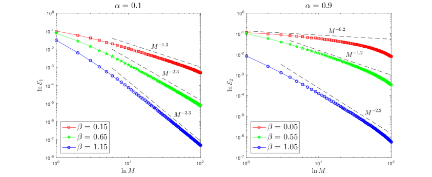
Figure 2: Temporal errors of 1 with $h=2^{-10}$.

Example 2.

To verify Theorem 4.2, we consider $f=0$ and

$$u_{0}(x):=\theta x(1-x)^{\gamma-1/2}+(1-\theta)\sin\pi x,\quad x\in\Omega,$$

where $\max\{-1,1-\frac{1}{\alpha}\}<\gamma<5/2$ and $\theta=0,1$. For $\theta=1$, a straightforward calculation yields that $u_{0}\in\dot{H}^{\gamma-\epsilon}(\Omega)$ for any $\epsilon>0$; and for $\theta=0$, we have $u_{0}=\sin\pi x\in\dot{H}^{\beta}(\Omega)$ with any $\beta>0$, since $\sin\pi x$ is an eigenfunction of $-\Delta$ on $\Omega=(0,1)$ with the homogeneous Dirichlet boundary condition. The convergence behaviour is plotted in Fig. 3, which implies that

$$\begin{split}\mathcal{E}_{1}={}&\left\{\begin{aligned} &O(M^{-1-\alpha(\gamma-1)}),&&-1/2<\gamma<3,\,\theta=1,\\ &O(M^{-1-2\alpha}),&&\theta=0,\end{aligned}\right.\\ \mathcal{E}_{2}={}&\left\{\begin{aligned} &O(M^{-1-\alpha(\gamma-1)}),&&-0.1<\gamma<2,\,\theta=1,\\ &O(M^{-1-\alpha}),&&\theta=0.\end{aligned}\right.\end{split}$$

These coincide with the sharp estimates established in Theorem 4.2.

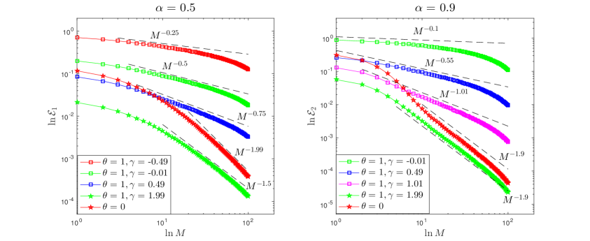
Figure 3: Temporal errors of 2 with $h=2^{-10}$.

Example 3.

This example is to verify Theorem 4.3 with $u_{0}=0$ and

$$f(x,t)=v(x):=x^{\gamma-1/2}(1-x),\quad x\in\Omega,$$

where $-1/2<\gamma<3/2$. It is evident that $v\in\dot{H}^{\gamma-\epsilon}(\Omega)$ for any $\epsilon>0$. Numerical results are displayed in Fig. 4, from which we conclude that

$$\begin{split}\mathcal{E}_{1}={}&\left\{\begin{aligned} &O(M^{-1-\alpha(\gamma+1)}),&&-1/2<\gamma<1,\\ &O(M^{-1-2\alpha}),&&1\leqslant\gamma<3/2,\end{aligned}\right.\\ \mathcal{E}_{2}={}&\left\{\begin{aligned} &O(M^{-1-\alpha(\gamma+1)}),&&-1/2<\gamma<0,\\ &O(M^{-1-\alpha}),&&0\leqslant\gamma<3/2.\end{aligned}\right.\end{split}$$

These are conformable to the sharp error bounds presented in Theorem 4.3.

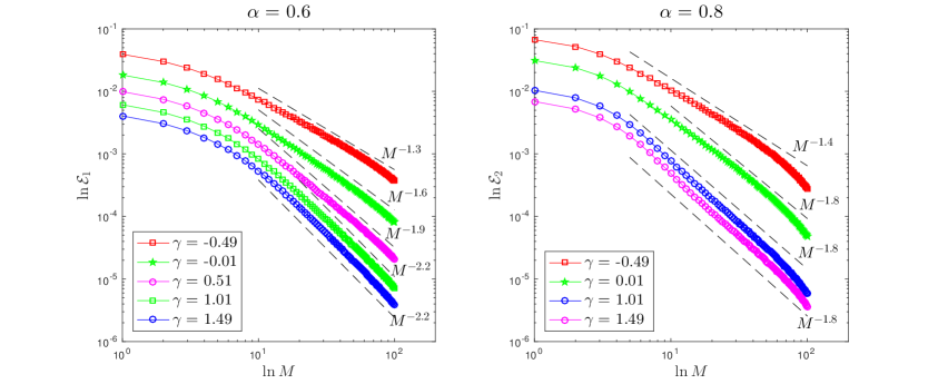
Figure 4: Temporal errors of 3 with $h=2^{-10}$.

6 Conclusion

This paper has concerned the sharp error estimation of the time-spectral algorithm for time fractional diffusion problems of order $\alpha$ ($0<\alpha<1$). Based on the new regularity results in the Besov space, optimal convergence rates of the numerical algorithm have been derived with low regularity data. Particularly, sharp temporal convergence orders $1+2\alpha$ and $1+\alpha$ under $L^{2}(0,T;\dot{H}^{1}(\Omega))$-norm and $H^{\alpha/2}(0,T;L^{2}(\Omega))$-norm have been shown theoretically and numerically.

Beyond the presented results, several problems are deserving further investigation. The first is to establish the error estimate under $L^{2}(0,T;L^{2}(\Omega))$-norm. We conjecture that, for both the homogenuous case that $f=0,\,u_{0}\in\dot{H}^{2}(\Omega)$ and the nonhomogeneous case that $u_{0}=0,\,f=v\in L^{2}(\Omega)$, the theoretical temporal accuracy under $L^{2}(0,T;L^{2}(\Omega))$-norm shall be $1+2\alpha$, which has been verified via our numerical tests (not displayed in the context). The second is to conquer the boundary singularity via some singular basis or log orthogonal function [6] and establish a rigorous error analysis for nonsmooth data.

Appendix A The Shifted Jacobi Polynomial

Given $a,b>-1$, the family of shifted Jacobi polynomial $\{S_{k}^{a,b}\}_{k=0}^{\infty}$ on $(0,T)$ are defined as follows:

$$\mu^{a,b}(t)S_{k}^{a,b}(t)=\frac{(-1)^{k}}{T^{k}k!}\frac{\,{\rm d}^{k}}{\,{\rm d}t^{k}}\mu^{k+a,k+b}(t),\quad 0<t<T,$$ (63)

where $\mu^{\nu,\theta}(t)=(T-t)^{\nu}t^{\theta}$ for all $-1<\nu,\theta<\infty$. Note that 63 is also called Rodrigues’ formula [56], which implies $\{S_{k}^{a,b}\}_{k=0}^{\infty}$ is orthogonal with respect to the weight $\mu^{a,b}$ on $(0,T)$, i.e.,

$$\left\langle{S_{k}^{a,b},S_{l}^{a,b}}\right\rangle_{\mu^{a,b}}=\xi_{k}^{a,b}\delta_{kl},$$ (64)

where $\delta_{kl}$ denotes the Kronecker product and

$$\xi_{k}^{a,b}:=\frac{T^{a+b+1}\Gamma(k+a+1)\Gamma(k+b+1)}{(2k+a+b+1)k!\Gamma(k+a+b+1)}.$$ (65)

As $\{S_{k}^{a,b}\}_{k=0}^{\infty}$ forms a complete orthogonal basis of $L^{2}_{\mu^{a,b}}(0,T)$, any $v\in L^{2}_{\mu^{a,b}}(0,T)$ admits a unique decomposition

$$v=\sum_{k=0}^{\infty}v_{k}S_{k}^{a,b}\quad\text{with }v_{k}=\frac{1}{\xi_{k}^{a,b}}\left\langle{v,S_{k}^{a,b}}\right\rangle_{\mu^{a,b}},$$

and the $L^{2}_{\mu^{a,b}}$-orthogonal projection of $v$ onto $P_{M}(0,T)$ is defined as

$$\Phi_{M}^{a,b}v:=\sum_{k=0}^{M}v_{k}S_{k}^{a,b}.$$

For ease of notation, we shall set $S_{k}^{a}=S_{k}^{a,a},\,\mu^{a}=\mu^{a,a},\,\Phi_{M}^{a}=\Phi_{M}^{a,a}$, and all the superscripts are omitted when $a=0$.

Thanks to [7, Lemma 2.4], a standard calculation gives

$$\operatorname{D}_{0+}^{-\theta}S_{k}^{\beta+\theta,0}={}\frac{k!}{\Gamma(k+1+\theta)}t^{\theta}S_{k}^{\beta,\theta}(t),\quad\operatorname{D}_{T-}^{-\theta}S_{k}^{0,\beta+\theta}={}\frac{k!}{\Gamma(k+1+\theta)}(T-t)^{\theta}S_{k}^{\theta,\beta}(t)$$ (66)

and

$$\operatorname{D}_{0+}^{\theta}S_{k}^{\beta-\theta,0}={}\frac{k!}{\Gamma(k+1-\theta)}t^{-\theta}S_{k}^{\beta,-\theta}(t),\quad\operatorname{D}_{T-}^{\theta}S_{k}^{0,\beta-\theta}={}\frac{k!}{\Gamma(k+1-\theta)}(T-t)^{-\theta}S_{k}^{-\theta,\beta}(t),$$ (67)

where $0<\theta<1$ and $-1<\beta<\infty$.

Lemma A.1.

For any $v\in H^{\alpha/2}(0,T)$, we have

$$\left\langle{\operatorname{D}_{0+}^{\alpha}(I-\Phi_{M}^{-\alpha,0})v,q}\right\rangle_{H^{\alpha/2}(0,T)}=0\quad\forall\,q\in P_{M}(0,T).$$ (68)

Consequently, it holds the stability

$$\left\lvert{\Phi_{M}^{-\alpha,0}v}\right\rvert_{H^{\alpha/2}(0,T)}\leqslant{} C_{\alpha}\left\lvert{v}\right\rvert_{H^{\alpha/2}(0,T)}.$$ (69)

Proof.

Given any $v\in H^{\alpha/2}(0,T)$, by [16, Theorem 1.4.4.3] it is clear that $v\in L_{\mu^{-\alpha,0}}^{2}(0,T)={\mathbb{B}}_{-\alpha,0}^{0}(0,T)$. Thus we have the orthogonal decomposition

$$v=\sum_{k=0}^{\infty}v_{k}S_{k}^{-\alpha,0},\quad v_{k}=\frac{1}{\xi_{k}^{-\alpha,0}}\left\langle{v,S_{k}^{-\alpha,0}}\right\rangle_{\mu^{-\alpha,0}},$$

where $\xi_{k}^{-\alpha,0}$ is given by 65, and the $L^{2}_{\mu^{-\alpha,0}}$-orthogonal projection of $v$ onto $P_{M}(0,T)$ is given by

$$\Phi_{M}^{-\alpha,0}v=\sum_{k=0}^{M}v_{k}S_{k}^{-\alpha,0}.$$

Hence, the projection error reads as

$$(I-\Phi_{M}^{-\alpha,0})v=\sum_{k=M+1}^{\infty}v_{k}S_{k}^{-\alpha,0}.$$

For any $q\in P_{M}(0,T)$, we rewrite it as an expansion of $\{S_{k}^{0,-\alpha}\}_{k=0}^{M}$:

$$q=\sum_{k=0}^{M}q_{k}S_{k}^{0,-\alpha},\quad q_{k}=\frac{1}{\xi_{k}^{0,-\alpha}}\left\langle{q,S_{k}^{0,-\alpha}}\right\rangle_{\mu^{0,-\alpha}},$$

where $\xi_{k}^{0,-\alpha}$ is defined by 65. From 67 we get

$$\operatorname{D}_{0+}^{\alpha/2}(I-\Phi_{M}^{-\alpha,0})v=\sum_{k=M+1}^{\infty}\frac{v_{k}k!}{\Gamma(k+1-\alpha/2)}t^{-\alpha/2}S_{k}^{-\alpha/2},$$

$$\operatorname{D}_{T-}^{\alpha/2}q=\sum_{k=0}^{M}\frac{q_{k}k!}{\Gamma(k+1-\alpha/2)}(T-t)^{-\alpha/2}S_{k}^{-\alpha/2}.$$

Applying Lemma 2.1 yields the equality

$$\left\langle{\operatorname{D}_{0+}^{\alpha}(I-\Phi_{M}^{-\alpha,0})v,q}\right\rangle_{H^{\alpha/2}(0,T)}=\left\langle{\operatorname{D}_{0+}^{\alpha/2}(I-\Phi_{M}^{-\alpha,0})v,\operatorname{D}_{T-}^{\alpha/2}q}\right\rangle_{(0,T)},$$

and it follows from the orthogonality of $\{S^{-\alpha/2}_{k}\}_{k=0}^{\infty}$ with respect to the weight $\mu^{-\alpha/2}$ that

$$\left\langle{\operatorname{D}_{0+}^{\alpha/2}(I-\Phi_{M}^{-\alpha,0})v,\operatorname{D}_{T-}^{\alpha/2}q}\right\rangle_{(0,T)}=0\quad\forall\,q\in P_{M}(0,T).$$

This shows 68. As 69 is a direct corollary of 68, we complete the proof of this lemma. ∎

Remark A.1.

Define the generalized Jacobi orthogonal projection

$$\pi_{M}^{-\alpha}:L^{2}_{\mu^{-\alpha}}(0,T)\longrightarrow\{t^{\alpha}\}\otimes P_{M}(0,T)$$

by that

$$\left\langle{(I-\pi_{M}^{-\alpha})v,q}\right\rangle_{\mu^{-\alpha}}=0\quad\forall\,q\in\{t^{\alpha}\}\otimes P_{M}(0,T)\quad\forall v\in L^{2}_{\mu^{-\alpha}}(0,T).$$

Then for any $v\in H^{\alpha/2}(0,T)$, we have an identity similar with 68 (see [7, Remark 4.3] or [55, Eq. 3.26]):

$$\left\langle{\operatorname{D}_{0+}^{\alpha}(I-\pi_{M}^{-\alpha})v,q}\right\rangle_{H^{\alpha/2}(0,T)}=0\quad\forall\,q\in P_{M}(0,T).$$

References

• [1] A. Abramovitz and I. Stegun. Handbook of Mathematical Functions. Dover, New York, 1972.
• [2] A. Alikhanov. A new difference scheme for the time fractional diffusion equation. J. Comput. Phys., 280:424–438, 2015.
• [3] I. Babuška and B. Guo. Direct and inverse approximation theorems for the $p$-version of the finite element method in the framework of weighted Besov spaces. part i: approximability of functions in the weighted Besov spaces. SIAM J. Numer. Anal., 39(5):1512–1538, 2002.
• [4] I. Babuška and M. Suri. The optimal convergence rate of the $p$-version of the finite element method. SIAM J. Numer. Anal., 24(4):750–776, 1987.
• [5] J. Bergh and J. Löfström. Interpolation Spaces: An Introduction. Number 223 in Die Grundlehren der mathematischen Wissenschaften in Einzeldarstellungen. Springer, Berlin, 1976.
• [6] S. Chen and J. Shen. Log orthogonal functions: approximation properties and applications. arXiv : 2003.01209, 2020.
• [7] S. Chen, J. Shen, and L. Wang. Generalized Jacobi functions and their applications to fractional differential equations. Math. Comp., 85(300):1603–1638, 2016.
• [8] B. Duan and Z. Zheng. An exponentially convergent scheme in time for time fractional diffusion equations with non-smooth initial data. J. Sci. Comput., 80(2):717–742, 2019.
• [9] V. Ervin and J. Roop. Variational formulation for the stationary fractional advection dispersion equation. Numer. Meth. Part. D. E., 22(3):558–576, 2006.
• [10] L. Evans. Partial Differential Equations, 2nd. Number 19 in Graduate Studies in Mathematics. American Mathematical Society, 2010.
• [11] N. Ford, J. Xiao, and Y. Yan. A finite element method for time fractional partial differential equations. Fract. Calc. Appl. Anal., 14(3):454–474, 2011.
• [12] N. Ford and Y. Yan. An approach to construct higher order time discretisation schemes for time fractional partial differential equations with nonsmooth data. Fract. Calc. Appl. Anal., 20(5):1076–1105, 2017.
• [13] G. Gao, H. Sun, and Z. Sun. Stability and convergence of finite difference schemes for a class of time-fractional sub-diffusion equations based on certain superconvergence. J. Comput. Phys., 280:510–528, 2015.
• [14] R. Gorenflo, J. Loutchko, and Y. Luchko. Computation of the Mittag–Leffler function ${E}_{\alpha,\beta}(z)$ and its derivative. Fract. Calc. Appl. Anal., 5(4):12–15, 2002.
• [15] R. Gorenflo, Y. Luchko, and M. Yamamoto. Time-fractional diffusion equation in the fractional Sobolev spaces. Fract. Calc. Appl. Anal., 18(3):799–820, 2015.
• [16] P. Grisvard. Elliptic Problems in Nonsmooth Domains. Pitman, London, 1985.
• [17] W. Gui and I. Babuška. The $h,p$ and $h$-$p$ versions of the finite element method in 1 dimension. Part I. The error analysis of the $p$-version. Numer. Math., 49(6):577–612, 1986.
• [18] B. Guo and L. Wang. Jacobi approximations in non-uniformly Jacobi-weighted Sobolev spaces. J. Approx. Theory, 128(1):1–41, 2004.
• [19] B. Jin, R. Lazarov, J. Pasciak, and Z. Zhou. Error analysis of semidiscrete finite element methods for inhomogeneous time-fractional diffusion. IMA J. Numer. Anal., 35(2):561–582, 2015.
• [20] B. Jin, R. Lazarov, and Z. Zhou. Error estimates for a semidiscrete finite element method for fractional order parabolic equations. SIAM J. Numer. Anal., 51(1):445–466, 2013.
• [21] B. Jin, R. Lazarov, and Z. Zhou. An analysis of the L1 scheme for the subdiffusion equation with nonsmooth data. IMA J. Numer. Anal., 36:197–221, 2015.
• [22] B. Jin, B. Li, and Z. Zhou. Correction of high-order BDF convolution quadrature for fractional evolution equations. SIAM J. Sci. Comput., 39(6):A3129–A3152, 2017.
• [23] A. Kilbas, H. Srivastava, and J. Trujillo. Theory and Applications of Fractional Differential Equations, 1st. Number 204 in North-Holland Mathematics Studies. Elsevier, Amsterdam, 2006.
• [24] N. Kopteva. Error analysis of an L2-type method on graded meshes for a fractional-order parabolic problem. arXiv:1905.05070, 2019.
• [25] B. Li, H. Luo, and X. Xie. Error estimates of a discontinuous Galerkin method for time fractional diffusion problems with nonsmooth data. arXiv: 1809.02015, 2018.
• [26] B. Li, H. Luo, and X. Xie. A time-spectral algorithm for fractional wave problems. J. Sci. Comput., 77(2):1164–1184, 2018.
• [27] B. Li, H. Luo, and X. Xie. Analysis of a time-stepping scheme for time fractional diffusion problems with nonsmooth data. SIAM J. Numer. Anal., 57(2):779–798, 2019.
• [28] B. Li, H. Luo, and X. Xie. A space-time finite element method for fractional wave problems. Numer. Algor., 85(3):1095–1121, 2020.
• [29] B. Li, T. Wang, and X. Xie. Analysis of a time-stepping discontinuous Galerkin method for fractional diffusion-wave equation with nonsmooth data. J. Sci. Comput., 82: 4, 2020.
• [30] B. Li, T. Wang, and X. Xie. Analysis of the L1 scheme for fractional wave equations with nonsmooth data. arXiv:1908.09145, 2019.
• [31] B. Li, T. Wang, and X. Xie. Analysis of a temporal discretization for a semilinear fractional diffusion equation. Computers & Mathematics with Applications,80(10): 2115–2134, 2020.
• [32] B. Li, T. Wang, and X. Xie. Numerical analysis of two Galerkin discretizations with graded temporal grids for fractional evolution equations. J. Sci. Comput., 85: 3, 2020.
• [33] B. Li and X. Xie. Regularity of solutions to time fractional diffusion equations. Discrete Contin. Dyn. Syst. -B, 24:3195–3210, 2019.
• [34] B. Li, X. Xie, and S. Zhang. A new smoothness result for Caputo-type fractional ordinary differential equations. Appl. Math. Comput., 349:408–420, 2019.
• [35] X. Li and C. Xu. A space-time spectral method for the time fractional diffusion equation. SIAM J. Numer. Anal., 47(3):2108–2131, 2019.
• [36] Y. Lin and C. Xu. Finite difference/spectral approximations for the time-fractional diffusion equation. J. Comput. Phys., 225(2):1533–1552, 2007.
• [37] J. Lions and E. Magenes. Non-Homogeneous Boundary Value Problems and Applications, Vol 3. Springer, Berlin, 1973.
• [38] Y. Luchko and A. Punzi. Modeling anomalous heat transport in geothermal reservoirs via fractional diffusion equations. GEM - International Journal on Geomathematics, 1(2):257–276, 2011.
• [39] A. Lunardi. Interpolation Theory. Springer, Basel, 1995.
• [40] H. Luo, B. Li, and X. Xie. Convergence analysis of a Petrov–Galerkin method for fractional wave problems with nonsmooth data. J. Sci. Comput., 80(2):957–992, 2019.
• [41] C. Lv and C. Xu. Error analysis of a high order method for time-fractional diffusion equations. SIAM J. Sci. Comput., 38(5):A2699–A2724, 2016.
• [42] W. McLean. Regularity of solutions to a time-fractional diffusion equation. ANZIAM., 52(2):123–138, 2010.
• [43] W. McLean and K. Mustapha. Convergence analysis of a discontinuous Galerkin method for a sub-diffusion equation. Numer. Algor., 52(1):69–88, 2009.
• [44] W. McLean and K. Mustapha. Time-stepping error bounds for fractional diffusion problems with non-smooth initial data. J. Comput. Phys., 293(C):201–217, 2015.
• [45] R. Metzler, W. Glöckle, and T. Nonnenmacher. Fractional model equation for anomalous diffusion. Physica A: Statistical Mechanics and its Applications, 211(1):13–24, 1994.
• [46] R. Metzler and J. Klafter. The random walk’s guide to anomalous diffusion: A fractional dynamics approach. Phys. Rep., 339(1):1–77, 2000.
• [47] G. Mittag-Leffler. Sur la nouvelle function ${E}_{\alpha}$. C. R. Acad. Sci. Paris, 137:554–558, 1903.
• [48] K. Mustapha. Time-stepping discontinuous Galerkin methods for fractional diffusion problems. Numer. Math., 130(3):497–516, 2015.
• [49] K. Mustapha, B. Abdallah, and K. Furati. A discontinuous Petrov–Galerkin method for time-fractional diffusion equations. SIAM J. Numer. Anal., 52(5):2512–2529, 2014.
• [50] K. Mustapha and W. McLean. Uniform convergence for a discontinuous Galerkin, time-stepping method applied to a fractional diffusion equation. IMA J. Numer. Anal., 32(3):906–925, 2012.
• [51] K. Mustapha and W. McLean. Superconvergence of a discontinuous Galerkin method for fractional diffusion and wave equations. SIAM J. Numer. Anal., 51(1):491–515, 2013.
• [52] I. Podlubny. Fractional Differential Equations, volume 198 of Mathematics in Science and Engineering. Academic Press, 1999.
• [53] A. Quarteroni and A. Valli. Numerical Approximation of Partial Differential Equations, 1st. Number 23 in Springer Series in Computational Mathematics. Springer, Berlin, 2008.
• [54] K. Sakamoto and M. Yamamoto. Initial value/boundary value problems for fractional diffusion-wave equations and applications to some inverse problems. J. Math. Anal. Appl., 382(1):426–447, 2011.
• [55] J. Shen and C. Sheng. An efficient space-time method for time fractional diffusion equation. J. Sci. Comput., 81(2):1088–1110, 2019.
• [56] J. Shen, T. Tang, and L. Wang. Spectral Methods: Algorithms, Analysis and Applications. Number 41 in Springer Series in Computational Mathematics. Springer, Heidelberg, 2011.
• [57] E. Stein and R. Shakarchi. Functional Analysis–Introduction to Further Topics in Analysis. Number 4 in Princeton Lectures in Analysis. Princeton University Press, Princeton, 2011.
• [58] M. Stynes, E. O’Riordan, and J. Gracia. Error analysis of a finite difference method on graded meshes for a time-fractional diffusion equation. SIAM J. Numer. Anal., 55(2):1057–1079, 2017.
• [59] L. Tartar. An Introduction to Sobolev Spaces and Interpolation Spaces. Number 3 in Lecture Notes of The Unione Matematica Italiana. Springer, Berlin, 2007.
• [60] Y. Xing and Y. Yan. A higher order numerical method for time fractional partial differential equations with nonsmooth data. J. Comput. Phys., 357:305–323, 2018.
• [61] Y. Yan, M. Khan, and N. Ford. An analysis of the modified L1 scheme for time-fractional partial differential equations with nonsmooth data. SIAM J. Numer. Anal., 56(1):210–227, 2018.
• [62] Y. Yang, Y. Yan, and N. Ford. Some time stepping methods for fractional diffusion problems with nonsmooth data. Comput. Meth. Appl. Mat., 18(1):129–146, 2018.
• [63] G. Zaslavsky. Chaos, fractional kinetics, and anomalous transport. Phys. Rep., 371(6):461–580, 2002.
• [64] M. Zheng, F. Liu, I. Turner, and V. Anh. A novel high order space-time spectral method for the time fractional Fokker–Planck equation. SIAM J. Sci. Comput., 37(2):A701–A724, 2015.