Preservation of the Global Knowledge by
Not-True Distillation in Federated Learning

Abstract

In federated learning, a strong global model is collaboratively learned by aggregating clients’ locally trained models. Although this precludes the need to access clients’ data directly, the global model’s convergence often suffers from data heterogeneity. This study starts from an analogy to continual learning and suggests that forgetting could be the bottleneck of federated learning. We observe that the global model forgets the knowledge from previous rounds, and the local training induces forgetting the knowledge outside of the local distribution. Based on our findings, we hypothesize that tackling down forgetting will relieve the data heterogeneity problem. To this end, we propose a novel and effective algorithm, Federated Not-True Distillation (FedNTD), which preserves the global perspective on locally available data only for the not-true classes. In the experiments, FedNTD shows state-of-the-art performance on various setups without compromising data privacy or incurring additional communication costs.

1 Introduction

At present, massive data is being collected from edge devices such as mobile phones, vehicles, and facilities. As the data may be distributed on numerous devices, decentralized training is often required to train deep network models. Federated learning [24, 23] is a distributed learning paradigm that enables the learning of a global model while preserving clients’ data privacy. In federated learning, clients independently train local models using their private data, and the server aggregates them into a single global model. In this process, most of the computation is performed by client devices, while the global server only aggregates the model parameters and distributes them to clients [2, 50].

Most federated learning algorithms are based on FedAvg [37], which aggregates the locally trained model parameters by weighted averaging proportional to the amount of local data that each client had. While various federated learning algorithms have been proposed thus far, they each conduct parameter averaging in a certain manner [30, 20, 47, 9, 52, 1]. Although this aggregation scheme empirically works well and provides a conceptually ideal framework when all client devices are active and i.i.d. distributed (a.k.a. LocalSGD), the data heterogeneity problem [31, 56] is a notorious challenge for federated learning applications and prevents their widespread applicability [29, 19].

As the clients generate their own data, the data is not identically distributed. More precisely, the local data across clients are drawn from heterogeneous underlying distributions; thereby, locally available data fail to represent the overall global distribution, which is referred to as data heterogeneity. Despite its inevitable occurrence in many real-world scenarios, data heterogeneity not only makes theoretical analysis difficult [31, 56] but also degrades many federated learning algorithms’ performances [18, 27]. By resolving the data heterogeneity problem, learning becomes more robust against partial participation [37, 31], and the communication cost is also reduced by faster convergence [46, 52].

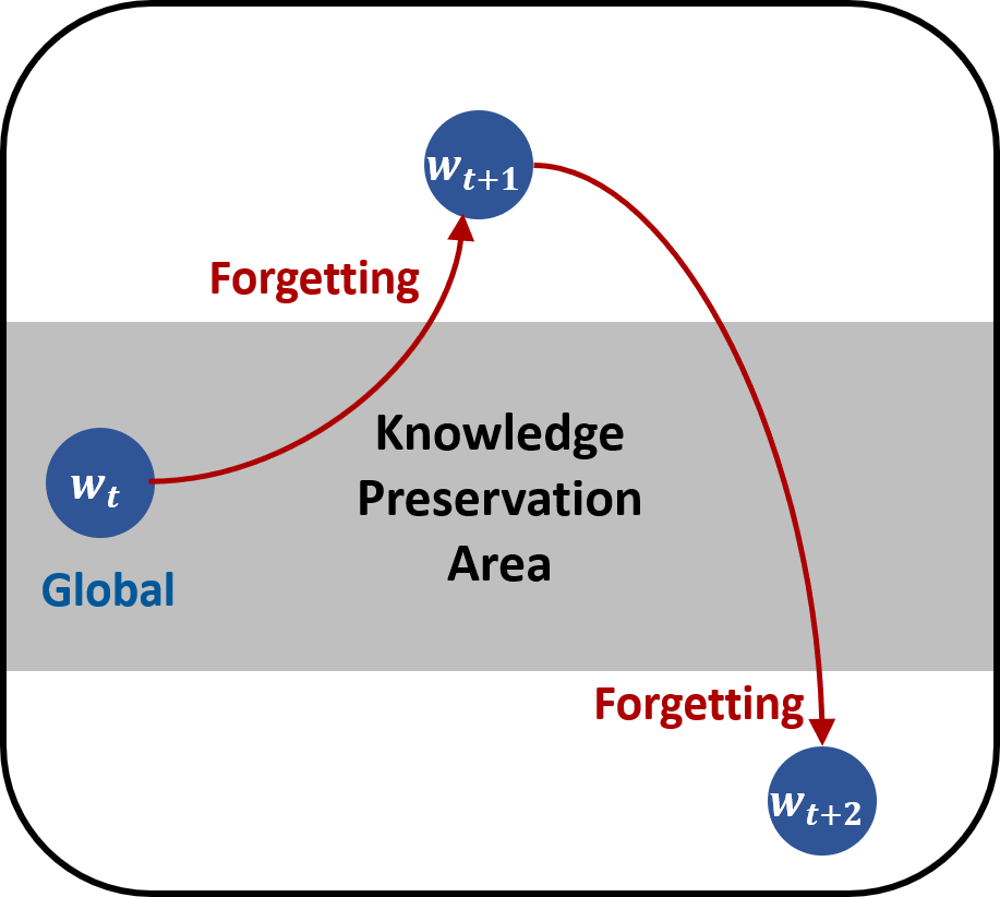
(a) Continual Learning

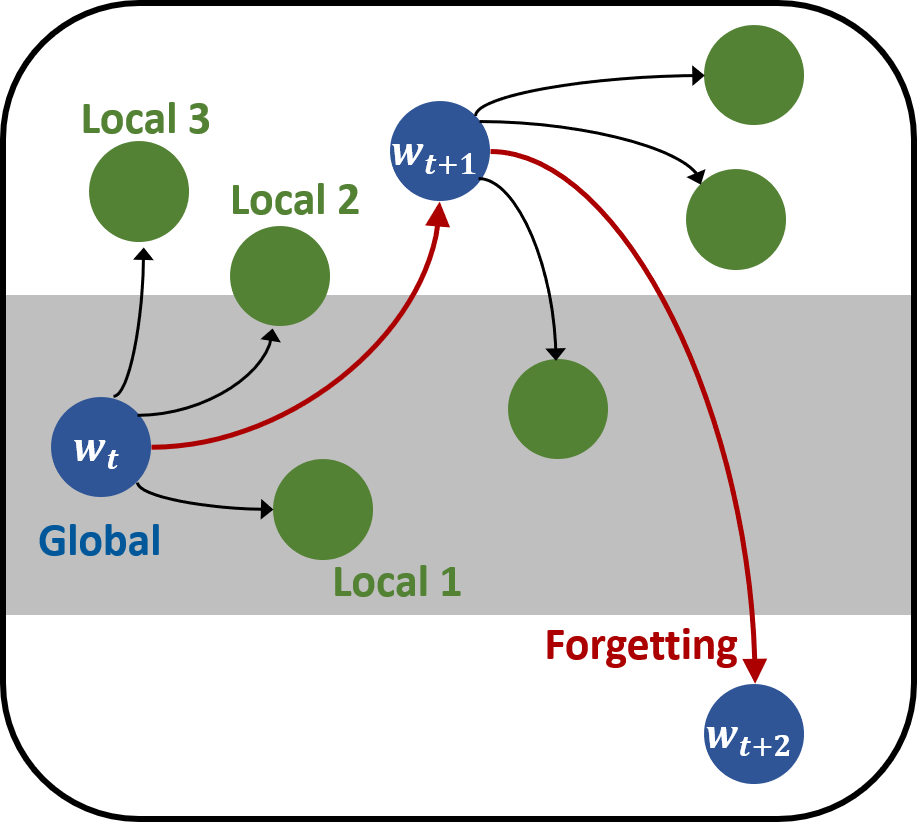
(b) Federated Learning (FedAvg)

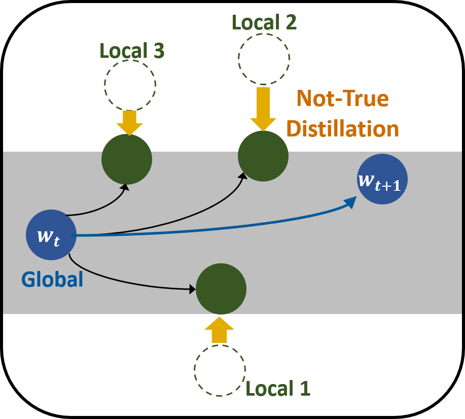
(c) Federated Learning (FedNTD)

Figure 1: An overview of forgetting in learning scenarios. As catastrophic forgetting in (a) Continual Learning, (b) Federated Learning also experiences forgetting. However, (c) FedNTD prevents forgetting by preserving global knowledge during local training.

Interestingly, continual learning [42, 45] faces a similar challenge. In continual learning, a learner model is continuously updated on a sequence of tasks, with an objective to perform well on whole tasks. Unfortunately, owing to the heterogeneous data distribution of each task, learning on the task sequence often results in catastrophic forgetting [40, 36], whereby fitting on a new task interferes with the parameters important for previous tasks. As a consequence, the model parameters drift away from the area where the previous knowledge is desirably preserved (1(a)).

Our first conjecture is such forgetting also exists in federated learning. While the server aggregates local models, the distribution where they are trained may be largely different from those of previous rounds. As a result, the global model faces the distributional shifts at each round, which may cause the forgetting as in continual learning (1(b)). To empirically verify this analogy, we examine the global model’s prediction consistency. More specifically, we measure its class-wise accuracy while the communication rounds proceed.

The observations verify our conjecture: the global model’s prediction is highly inconsistent across communication rounds, significantly reducing the performance of predicting some classes that the previous model originally predicted well. We dig deeper to analyze how averaging the locally updated parameters induces such forgetting and confirm that it occurs in local training: the global knowledge, corresponding to the region outside of local distribution, is prone to be forgotten. As merely averaging the local models cannot recover it, the global model struggles to preserve previous knowledge.

Based on our findings, we hypothesize that mitigating the issue of forgetting can relieve data heterogeneity (1(c)). To this end, we propose a novel algorithm Federated Not-True Distillation (FedNTD). FedNTD utilizes the global model’s prediction on locally available data, but only for the not-true classes. We demonstrate the effect of FedNTD on preserving global knowledge outside of a local distribution and its benefits on federated learning. Experimental results show that FedNTD achieves state-of-the-art performance in various setups.

To summarize, our contributions as follows:

• We present a systematic study on forgetting in federated learning. The global knowledge outside of the local distribution is prone to be forgotten and is closely related to the data heterogeneity issue (Section 2).

• We propose a simple yet effective algorithm, FedNTD, to prevent forgetting. Unlike prior works, FedNTD neither compromises data privacy nor incurs additional communication burdens. We validate the efficacy of FedNTD on various setups and show that it consistently achieves state-of-the-art performance (Section 3, Section 4).

• We analyze how FedNTD benefits federated learning. The knowledge preservation by FedNTD improves weight alignment and weight divergence after local training (Section 5).

1.1 Preliminaries

Federated Learning

We aim to train an image classification model in a federated learning system that consists of $K$ clients and a central server. Each client $k$ has a local dataset $\mathcal{D}^{k}$, where the whole dataset $\mathcal{D}=\bigcup_{k\in[K]}\mathcal{D}^{k}$. At each communication round $t$, the server distributes the current global model parameters $w^{(t-1)}$ to sampled local clients $K^{(t)}$. Starting from $w^{(t-1)}$, each client $k\in K^{(t)}$ updates the model parameters $w_{k}^{(t)}$ using its local datasets $\mathcal{D}^{k}$ with the following objective:

$$w_{k}^{(t)}=\underset{w}{\text{argmin}}\>\>\mathbb{E}_{(x,y)\sim\mathcal{D}^{k}}[\mathcal{L}(w;w^{(t-1)},x,y)]\,.$$ (1)

where $\mathcal{L}$ is the loss function. At the end of round $t$, the sampled clients upload the locally updated parameters back to the server and aggregate by parameter averaging as $w^{(t)}$ as follows:

$$w^{(t)}=\sum_{k\in K^{(t)}}\frac{|\mathcal{D}^{k}|}{\sum_{k^{\prime}\in K^{(t)}}|\mathcal{D}^{k^{\prime}}|}\ w_{k}^{(t)}.$$ (2)

Knowledge Distillation

Given a teacher model $T$ and a student model $S$, knowledge distillation [17] matches their softened probability $q_{\mathcal{\tau}}^{T}$ and $q_{\mathcal{\tau}}^{S}$ using temperature $\tau$. The $c$-th value of the $q_{\tau}$ can be described as $q_{\tau}(c)=\frac{{\exp({z}_{c}/\tau)}}{{\sum_{i}\exp({z}_{i}/\tau)}}$, where $z_{c}$ is the $c$-th value of logits vector $z$ and $\mathcal{C}$ is the number of classes. Given a sample $x$, the student model $S$ is learned by a linear combination of cross-entropy loss $\mathcal{L}_{\textup{CE}}$ for one-hot label $\mathds{1}_{y}$ and Kullback-Leibler divergence loss $\mathcal{L}_{\textup{KL}}$ using a hyperparameter $\beta$:

$$\mathcal{L}=(1-\beta)\mathcal{L}_{\textup{CE}}(q,\mathds{1}_{y})+\beta{\tau}^{2}\mathcal{L}_{\textup{KL}}(q_{\mathcal{\tau}}^{S},q_{\mathcal{\tau}}^{T})$$ (3)

$$\mathcal{L}_{\textup{CE}}(q,\mathds{1}_{y})=-\sum_{c=1}^{\mathcal{C}}\mathds{1}_{y}(c)\log q(c),\qquad\mathcal{L}_{\textup{KL}}(q_{\mathcal{\tau}}^{S},q_{\mathcal{\tau}}^{T})=-\sum_{c=1}^{\mathcal{C}}{q}_{\tau}^{T}(c)\log\left[\frac{{q}_{\tau}^{S}(c)}{{q}_{\tau}^{T}(c)}\right]$$ (4)

2 Forgetting in Federated Learning

To understand how the non-IID data affects federated learning, we performed an experimental study on heterogeneous locals. We choose CIFAR-10 [25] and a convolutional neural network with four layers as in [37]. We split the data to 100 clients using Latent Dirichlet Allocation (LDA), assigning the partition of class $c$ samples to clients by $p\sim\text{Dir}(\alpha)$. The heterogeneity level increases as the $\alpha$ decreases. We train the model with FedAvg for 200 communication rounds, and 10 randomly sampled clients are optimized for 5 local epochs at each round. More details are in Appendix B.

2.1 Global Model Prediction Consistency

To confirm our conjecture on forgetting, we first consider how the global model’s prediction varies as the communication rounds proceed. If the data heterogeneity induces forgetting, the prediction after update (i.e., parameter averaging) may be less consistent compared to the previous round. To examine it, we observe the model’s class-wise test accuracy at each round, and measure its similarity to the previous round. The results are provided in Figure 2a and Figure 2b.

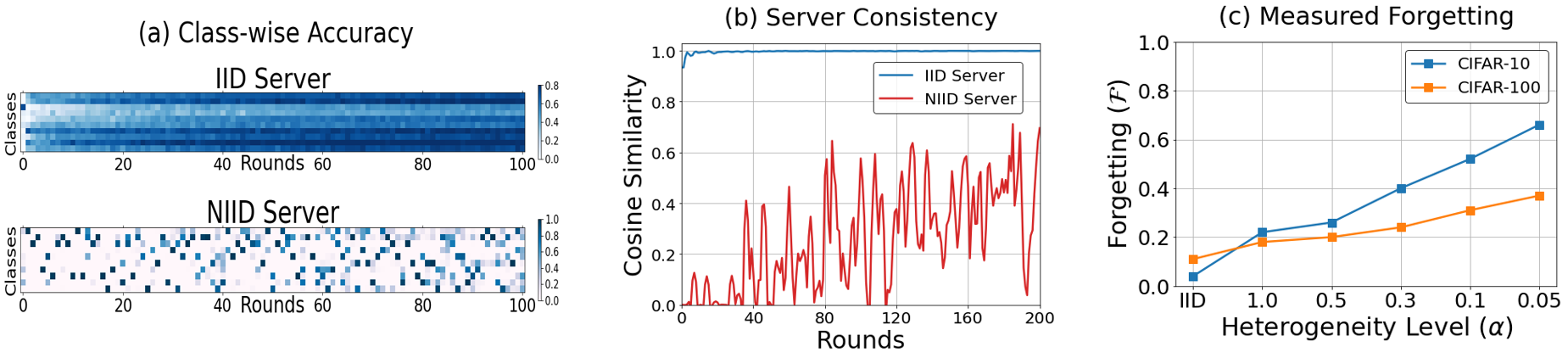
Figure 2: Forgetting analysis on the global server model. (a): Class-wise test accuracy on CIFAR-10 IID and NIID ($\alpha$=0.1) cases. (b): Cosine similarity of class-wise accuracy vector w.r.t. previous round global model on IID and NIID ($\alpha=0.1$) cases. (c): Forgetting $\mathcal{F}$ by different heterogeneity levels on CIFAR-10 and CIFAR-100.

As expected, while the server model learned from i.i.d. locals (IID Server) predicts each class evenly well at each round, prediction is highly inconsistent in the non-i.i.d. case (NIID Server). In the non-IID case, the test accuracy on some classes which originally predicted well by the previous global model often drops significantly. This implies that forgetting occurs in federated learning.

To measure how the forgetting is related to data heterogeneity, we borrow the idea of Backward Transfer (BwT) [5], a prevalent forgetting measure in continual learning [8, 4, 7, 14], as follows:

$$\mathcal{F}=\frac{1}{\mathcal{C}}\sum_{c=1}^{\mathcal{C}}\max_{t\in\{1,\dots\mathcal{T}-1\}}(\mathcal{A}_{c}^{(t)}-\mathcal{A}_{c}^{(\mathcal{T})})$$ (5)

where $\mathcal{A}_{c}^{(t)}$ is the accuracy on class $c$ at round $t$. Note that the forgetting measure, $\mathcal{F}$, captures the averaged gap between peak accuracy and the final accuracy for each class at the end of learning. The result on the varying heterogeneity levels is plotted in Figure 2c, showing that the global model suffers from forgetting more severely as the heterogeneity level increases.

2.2 Knowledge Outside of Local Distribution

We take a closer look at local training to investigate why aggregating the local models induces forgetting. In the continual learning view, a straightforward approach is to observe how fitting on the new distribution degrades the performance of the old distribution. However, in our problem setting, the local clients can have any class. Given that only their portions in the local distribution differ across clients, such strict comparison is intractable. Hence, we formulate in-local distribution $p(\mathcal{D})$ and its out-local distribution $\tilde{p}(\mathcal{D})$ to systematically analyze forgetting in local training.

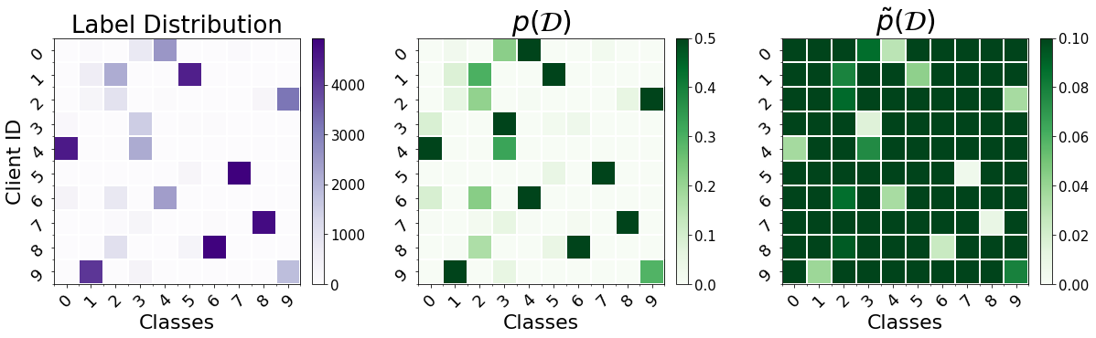
Figure 3: An example of in-local distribution $p(\mathcal{D})$ and out-local distribution $\tilde{p}(\mathcal{D})$ on CIFAR-10 ($\alpha=0.1$).

Definition 1.

Consider a local dataset $\mathcal{D}$ consists of $N$ data points $x_{i}$ and its label $y_{i}$ in $\mathcal{C}$-class classification problem. The in-local distribution vector $p^{k}=p(\mathcal{D}^{k})$ and its out-local distribution vector $\tilde{p}^{k}=\tilde{p}(\mathcal{D}^{k})$ are

$$p=[p_{1}\,,\ldots,p_{\mathcal{C}}],\quad \textup{where}\>\>p_{c}\coloneqq\frac{1}{N}\sum_{i=1}^{N}\mathbb{I}(y_{i}=c)$$ (6)

$$\tilde{p}=[\tilde{p}_{1}\,,\ldots,\tilde{p}_{\mathcal{C}}],\quad \textup{where}\>\>\tilde{p}_{c}\coloneqq\frac{1}{\mathcal{C}-1}(1-p_{c})$$ (7)

The underlying idea of out-local distribution $\tilde{p}(\mathcal{D})$ is to assign a higher proportion to the classes with fewer samples in local datasets. Accordingly, it corresponds to the region in the global distribution where the in-local distribution $p(\mathcal{D})$ cannot represent. Note that if $p(\mathcal{D})$ is uniform, $\tilde{p}(\mathcal{D})$ also collapses to uniform, which aligns well intuitively. An example of label distribution for 10 clients and their $p(\mathcal{D})$s and $\tilde{p}(\mathcal{D})$s are provided in Figure 3.

We measure the change of global and local models’ accuracy on $p(\mathcal{D})$ and $\tilde{p}(\mathcal{D})$ during each communication round, as in Figure 4. After local training, the local models are well-fitted towards $p(\mathcal{D})$ (Figure 4a), and the aggregated global model also performs well on it. On the other hand, the accuracy on $\tilde{p}(\mathcal{D})$ significantly drops, and the global model accuracy on it also degrades (Figure 4b).

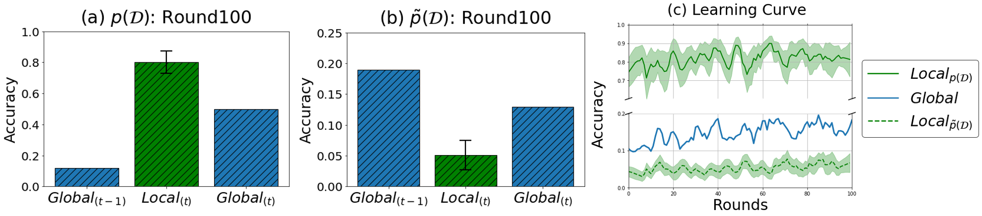
Figure 4: Accuracy of global model and sampled local models for $p(\mathcal{D})$ and $\tilde{p}(\mathcal{D})$ on CIFAR-10 ($\alpha$=0.1). The error bar stands for the standard deviation of the 10 sampled local clients. In (a) and (b), the global model accuracies for $p(\mathcal{D})$ and $\tilde{p}(\mathcal{D})$ is measured on their joint distributions from 10 sampled clients.

To summarize, the knowledge on the out-local distribution $\tilde{p}(\mathcal{D})$ is prone to be forgotten in local training, resulting in the global model’s forgetting. Based on our findings, we hypothesize that forgetting could be the stumbling block in federated learning.

2.3 Forgetting and Local Drift

First empirically observed by [56], the deviation of local updates from the desirable global direction has been widely discussed as a major cause of slow and unstable convergence in heterogeneous federated learning [21, 30, 31]. Unfortunately, given the difficulty of analyzing such drift, a common approach is to assume bounded dissimilarity between the local function gradients [20, 31].

One intriguing property of knowledge preservation on out-local distribution is that it corrects the local gradients towards the global direction. We define the gradient diversity $\Lambda$ to measure the dissimilarity of local gradients and state the effect of knowledge preservation as follows:

Definition 2.

For the uniformly weighted $K$ clients, the gradient diversity $\Lambda$ of local functions $f^{k}$ towards the global function $f=\frac{1}{K}\sum_{k=1}^{K}f^{k}$ is defined as:

$$\Lambda\mathrel{\mathop{\mathchar 58\relax}}=\frac{\frac{1}{K}\sum_{k=1}^{K}\lVert\nabla f^{k}\rVert^{2}}{\lVert\nabla f\rVert^{2}}\,$$ (8)

Here, $\Lambda\geq 1$ measures the alignment of gradient direction of the local function $f^{k}$s w.r.t. the global function $f$. Note that the $\Lambda$ becomes smaller as the directions of local function gradients $\nabla f^{k}$s become similar—e.g., if the magnitudes of the $\lVert\nabla f^{k}\rVert^{2}$s are fixed, the smallest $\Lambda$ is obtained when the direction of $\nabla f^{k}$s are identical. To understand the effect of preserving knowledge on the out-local distribution $\tilde{p}(\mathcal{D})$, we analyze how the local gradients and their diversity varies by adding gradient signal on $\tilde{p}(\mathcal{D})$ with factor $\beta$ and obtain the following proposition.

Proposition 1.

Suppose uniformly weighted $K$ clients with in-local distribution $p^{k}=[p^{k}_{1},\dots,p^{k}_{\mathcal{C}}]$. If we assume the class-wise gradients $g_{c}$ are orthogonal with uniform magnitude, increasing $\beta\leq\mathcal{C}/2-1$ reduces the gradient diversity $\Lambda$ from the local gradient $\nabla f^{k}=(p^{k}+\beta\tilde{p}^{k})\cdot g$ with the ratio:

$$\frac{\partial\Lambda}{\partial\beta}\>\>\leq\>\>-\frac{M_{K,\mathcal{C},p}}{(1+\beta)^{2}}\,.$$ (9)

where $\beta$ stands for the effect of knowledge preservation on the out-local distribution $\tilde{p}^{k}$. The $M_{K,\mathcal{C},p}>0$ is a constant term consists of $K$, $\mathcal{C}$, and $(p^{k})_{k=1}^{K}$ ,

The proof is given in Appendix P. Note that here we treat $f^{k}$ as a sum of class-wise losses $\sum_{c}p^{k}_{c}\mathcal{L}_{c}$, where $\mathcal{L}_{c}=\mathbb{E}_{x|y=c}[\mathcal{L}(x;w)]$ is the loss on the specific class $c$. When $\beta=0$, there is no regularization to preserve out-distribution knowledge, so the local model only needs to fit on the in-local distribution $p^{k}$. The above proposition suggests that the preserved knowledge on out-local distribution $\tilde{p}^{k}$ (i.e., as $\beta$ increases) guides the local gradient directions to be more aligned towards the global gradient, reducing the gradient diversity $\Lambda$. Such forgetting perspective provides the opportunity to handle the data heterogeneity at the model’s prediction level.

3 FedNTD: Federated Not-True Distillation

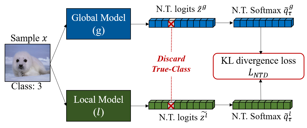
Figure 5: An overview of Not-True Distillation.The true class (Class 3) logits is ignored in the softmax.

In this section, we propose Federated Not-True Distillation (FedNTD) and its key features. The core idea of FedNTD is to preserve the global view only for the not-true classes. More specifically, FedNTD conducts local-side distillation by the linearly combined loss function $\mathcal{L}$ between the cross-entropy loss $\mathcal{L}_{\textup{CE}}$ and the not-true distillation loss $\mathcal{L}_{\textup{NTD}}$:

$$\mathcal{L}=\mathcal{L}_{\textup{CE}}(q^{l},\;\mathds{1}_{y})+\beta\cdot\mathcal{L}_{\textup{NTD}}({\tilde{q}_{\tau}^{l}},\;{\tilde{q}_{\tau}^{g}}).$$ (10)

Here, the hyperparameter $\beta$ stands for the strength of knowledge preservation on the out-local distribution. Then, the not-true distillation loss $\mathcal{L}_{\textup{NTD}}$ is defined as the KL-Divergence loss between the not-true softmax prediction vector ${\tilde{q}_{\tau}}^{l}$ and ${\tilde{q}_{\tau}^{g}}$ as follows:

$$\small{\mathcal{L}}_{\text{NTD}}({\tilde{q}_{\tau}^{l}},{\tilde{q}_{\tau}^{g}})=-\!\sum_{c=1\,,\underline{\mathbf{c\neq y}}}^{C}{\tilde{q}_{\tau}^{g}}(c)\log\left[\frac{{\tilde{q}_{\tau}^{l}}(c)}{{\tilde{q}_{\tau}^{g}}(c)}\right]\,,\>\>\text{where}\>\>\begin{cases}\normalsize{\tilde{q}_{\tau}^{l}}(c)=\frac{\exp{({z}_{c}^{l}/\tau)}}{\sum_{\underline{\mathbf{\tilde{c}\neq y}}}^{C}\exp{({z}_{\tilde{c}}^{l}/\tau)}}\vspace{8pt}\\ {\tilde{q}_{\tau}^{g}}(c)=\frac{\exp{({z}_{c}^{g}/\tau)}}{\sum_{\underline{\mathbf{\tilde{c}\neq y}}}^{C}\exp{({z}_{\tilde{c}}^{g}/\tau)}}\end{cases}\!\!(\forall c\neq y).$$ (11)

which take softmax with temperature $\tau$ only for the not-true class logits. Figure 5 illustrates how the not-true distillation works given a sample $x$. Note that ignoring the true-class logits makes gradient signal of $\mathcal{L}_{\textup{NTD}}$ to the true-class as $0$. The detailed algorithm is provided in Algorithm 1.

Algorithm 1 Federated Not-True Distillation (FedNTD)

Input: total rounds ${T}$, local epochs ${E}$, dataset $\mathcal{D}$, sampled clients sets ${K}^{(t)}\subset K$ in round $t$, learning rate $\gamma$

Initialize $w^{(}0)$ for global server weight

for each communication round $t=1,\cdots,T$ do

Server samples clients $K^{(t)}$ and broadcasts ${\tilde{w}}^{(t)}\leftarrow{w}^{(t)}$

for each client $k\in K^{(t)}$ in parallel do

for Local Steps $e=1\cdots E$ do

for Batches $j=1\cdots B$ do

${\tilde{w}}^{(t)}_{k}\leftarrow{\tilde{w}}^{(t)}_{k}-\gamma\nabla_{w}\mathcal{L}(\,\tilde{w}^{(t)}_{k}\,;\,[\,\mathcal{D}^{k}\,]_{j}\,)$       Using   [Equation 10]

end for

end for

end for

Upload ${\tilde{w}}^{t}_{k}$ to server

Server Aggregation :${w}^{(t+1)}\leftarrow\frac{1}{|K^{(t)}|}\sum_{k\in K^{(t)}}{\tilde{w}}^{(t)}_{k}$

end for

Server output : $w_{T}$

We now explain how learning to minimize $\mathcal{L}_{\textup{NTD}}$ preserves global knowledge on out-local distribution $\tilde{p}(\mathcal{D})$. Suppose there are $N$ number of data points in the local dataset $\mathcal{D}$. The accumulated Kullback-Leibler divergence loss $\mathcal{L}_{\textup{KL}}$ between $q_{\tau}^{l,i}$, the probability vector for the data $x_{i}$, and its reference $q_{\tau}^{g,i}$ to be matched for is:

$$\small\mathcal{L}_{\textup{KL}}=-\frac{1}{N}\sum_{i=1}^{N}\sum_{c=1}^{\mathcal{C}}q_{\tau}^{g,i}(c)\log\left[\frac{q_{\tau}^{l,i}(c)}{q_{\tau}^{g,i}(c)}\right]\,.$$ (12)

By splitting the summands for the true and not-true classes, the term becomes:

$$\small\mathcal{L}_{\textup{KL}}^{\textup{true}}=-\frac{1}{N}\sum_{i=1}^{N}q_{\tau}^{g,i}(y_{i})\log\left[\frac{q_{\tau}^{l,i}(y_{i})}{q_{\tau}^{g,i}(y_{i})}\right]\,,\,\mathcal{L}_{\textup{KL}}^{\textup{not-true}}=-\frac{1}{N}\sum_{i=1}^{N}\sum_{c^{\prime}\neq y_{i}}^{\mathcal{C}}q_{\tau}^{g,i}(c^{\prime})\log\left[\frac{q_{\tau}^{l,i}(c^{\prime})}{q_{\tau}^{g,i}(c^{\prime})}\right]\,.$$ (13)

Proposition 2.

Consider the in-local distribution $p(\mathcal{D})=[p_{1}\dots p_{\mathcal{C}}]$ such that $p_{c}=\frac{|\mathcal{S}_{c}|}{N}$ and its out-local distribution $\tilde{p}(\mathcal{D})=[\tilde{p}_{1},\dots\tilde{p}_{\mathcal{C}}]$, where $\mathcal{S}_{c}$ is the set of indices satisfying $y_{i}=c$. Then the $\mathcal{L}_{\textup{KL}}^{\textup{true}}$ and $\mathcal{L}_{\textup{KL}}^{\textup{not-true}}$ each are equivalent to the weighted sum on $p(\mathcal{D})$ and $\tilde{p}(\mathcal{D})$ as

$$\mathcal{L}_{\textup{KL}}^{\textup{true}}=\mathop{\raisebox{0.0pt}{\scalebox{1.8}{$\displaystyle\sum$}}}_{c=1}^{\mathcal{C}}\> {\color[rgb]{0.7,0,0}\boldsymbol{p_{c}}}\>\scalebox{1.35}{$\mathbb{E}_{i\in\mathcal{S}_{c}}$}\!\left[-{q_{\tau}^{g,i}(c)\log\left[\frac{q_{\tau}^{l,i}(c)}{q_{\tau}^{g,i}(c)}\right]}\right]$$

$$\frac{\mathcal{L}_{\textup{KL}}^{\textup{not-true}}}{\mathcal{C}-1}=\mathop{\raisebox{0.0pt}{\scalebox{1.8}{$\displaystyle\sum$}}}_{c=1}^{\mathcal{C}}\> {\color[rgb]{0.7,0,0}\tilde{\boldsymbol{p_{c}}}}\>\scalebox{1.35}{$\mathbb{E}_{i\notin\mathcal{S}_{c}}$}\!\left[-{q_{\tau}^{g,i}(c)\log\left[\frac{q_{\tau}^{l,i}(c)}{q_{\tau}^{g,i}(c)}\right]}\right]$$

With a minor amount of calculation from Equation 13, we derive the above proposition. The derivation is provided in Appendix Q. The proposition suggests that matching the true-class and the not-true class logits collapses to the loss on the in-local distribution $p(\mathcal{D})$ and the out-local distribution $\tilde{p}(\mathcal{D})$.

In the loss function of our FedNTD (Equation 10), we attain the new knowledge on the in-local distribution by following the true-class signals from the labeled data in local datasets using the $\mathcal{L}_{\textup{CE}}$. In the meanwhile, we preserve the previous knowledge on the out-local distribution by following the global model’s perspective, corresponding to the not-true class signals, using the $\mathcal{L}_{\textup{NTD}}$. Here, the hyperparameter $\beta$ controls the trade-off between learning on the new knowledge and preserving previous knowledge. This resembles to the stability-plasticity dilemma [39] in continual learning, where the learning methods must balance retaining knowledge from previous tasks while learning new knowledge for the current task [35].

4 Experiment

4.1 Experimental Setup

We test our algorithm on MNIST [11], CIFAR-10 [25], CIFAR-100 [25], and CINIC-10 [10]. We distribute the data to 100 clients and randomly sample clients with a ratio of 0.1. For CINIC-10, we use 200 clients, with a sampling ratio of 0.05. We use a momentum SGD with an initial learning rate of 0.1, and the momentum is set as 0.9. The learning rate is decayed with a factor of 0.99 at each round, and a weight decay of 1e-5 is applied. We adopt two different NIID partition strategies:

• (i) Sharding [37]: sort the data by label and divide the data into same-sized shards, and control the heterogeneity by $s$, the number of shards per user. In this strategy only considers the statistical heterogeneity as the dataset size is identical for each client. We set $s$ as MNIST ($s=2$), CIFAR-10 ($s\in\{2,3,5,10\}$), CIFAR-100 ($s=10$), and CINIC-10 ($s=2$).

• (ii) Latent Dirichlet Allocation (LDA) [34, 46]: assigns partition of class $c$ by sampling $p_{c}\approx\text{Dir}(\alpha)$. In this strategy, both the distribution and dataset size are different for each client. We set $\alpha$ as MNIST ($\alpha=0.1$), CIFAR-10 ($\alpha\in\{0.05,0.1,0.3,0.5\}$), CIFAR-100 ($\alpha=0.1$), and CINIC-10 ($\alpha=0.1$)

More details on model, datasets, hyperparameters, and partition strategies are provided in Appendix B.

Table 1: Accuracy@1 (%) on MNIST [11], CIFAR-10 [25], CIFAR-100 [25], and CINIC-10 [10]. The values in the parenthesis are forgetting measure $\mathcal{F}$. The arrow ($\downarrow$,  $\uparrow$)  shows the comparison to the FedAvg. The standard deviation of each experiment is provided in Appendix F.

NIID Partition Strategy : Sharding
Method	MNIST	CIFAR-10				CIFAR-100	CINIC-10
		$s=2$	$s=3$	$s=5$	$s=10$
FedAvg [37]	78.63${}_{(0.20)}\;\;$	40.14${}_{(0.59)}\;\;$	51.10${}_{(0.46)}\;\;$	57.17${}_{(0.37)}\;\;$	64.91${}_{(0.26)}\;\;$	25.57${}_{(0.49)}\;\;$	39.64${}_{(0.59)}\;\;$
FedCurv [43]	78.56(0.21) $\downarrow$	44.52(0.53) $\uparrow$	49.00(0.47) $\downarrow$	54.61(0.39) $\downarrow$	62.19(0.27) $\downarrow$	22.89(0.49) $\downarrow$	40.45(0.57) $\uparrow$
FedProx [30]	78.26(0.21) $\downarrow$	41.48(0.57) $\uparrow$	51.65(0.45) $\uparrow$	56.88(0.37) $\downarrow$	64.65(0.25) $\downarrow$	25.10(0.49) $\downarrow$	41.47(0.57) $\uparrow$
FedNova [47]	77.04(0.21) $\downarrow$	42.62(0.56) $\uparrow$	52.03(0.44) $\uparrow$	62.14(0.30) $\uparrow$	66.97(0.20) $\uparrow$	26.96(0.41) $\uparrow$	42.55(0.56) $\uparrow$
SCAFFOLD [20]	81.05(0.17) $\uparrow$	44.60(0.53) $\uparrow$	54.26(0.39) $\uparrow$	65.74(0.23) $\uparrow$	68.97(0.16) $\uparrow$	30.82(0.36) $\uparrow$	42.66(0.54) $\uparrow$
MOON [28]	76.56(0.23) $\downarrow$	38.51(0.60) $\downarrow$	50.47(0.47) $\downarrow$	56.69(0.39) $\downarrow$	65.30(0.25) $\uparrow$	25.29(0.48) $\downarrow$	37.07(0.62) $\downarrow$
FedNTD (Ours)	84.44(0.13) $\uparrow$	52.61(0.43) $\uparrow$	58.18(0.34) $\uparrow$	64.93(0.23) $\uparrow$	68.56(0.15) $\uparrow$	31.69(0.32) $\uparrow$	48.07(0.48) $\uparrow$
NIID Partition Strategy : LDA
Method	MNIST	CIFAR-10				CIFAR-100	CINIC-10
		$\alpha=0.05$	$\alpha=0.1$	$\alpha=0.3$	$\alpha=0.5$
FedAvg [37]	79.73${}_{(0.19)}\;\;$	28.24${}_{(0.71)}\;\;$	46.49${}_{(0.51)}\;\;$	57.24${}_{(0.36)}\;\;$	62.53${}_{(0.28)}\;\;$	30.69${}_{(0.32)}\;\;$	38.14${}_{(0.60)}\;\;$
FedCurv [43]	78.72(0.20) $\downarrow$	33.64(0.66) $\uparrow$	44.26(0.53) $\downarrow$	54.93(0.38) $\downarrow$	59.37(0.30) $\downarrow$	29.16(0.32) $\downarrow$	36.69(0.61) $\downarrow$
FedProx [30]	79.25(0.19) $\downarrow$	37.19(0.62) $\uparrow$	47.65(0.49) $\uparrow$	57.35(0.35) $\uparrow$	62.39(0.27) $\downarrow$	30.60(0.32) $\downarrow$	39.47(0.58) $\uparrow$
FedNova [47]	60.37(0.38) $\downarrow$	10.00 (Failed) $\downarrow$	28.06(0.71) $\downarrow$	57.44(0.35) $\uparrow$	64.65(0.23) $\uparrow$	32.15(0.28 $\uparrow$	30.44(0.68) $\downarrow$
SCAFFOLD [20]	71.57(0.26) $\downarrow$	10.00 (Failed) $\downarrow$	23.12(0.74) $\downarrow$	62.01(0.29) $\uparrow$	66.16(0.19) $\uparrow$	33.68(0.25) $\uparrow$	28.78(0.69) $\downarrow$
MOON [28]	78.95(0.20) $\downarrow$	28.35(0.71) $\uparrow$	44.77(0.53) $\downarrow$	58.38(0.35) $\uparrow$	63.10(0.27) $\uparrow$	30.64(0.32) $\downarrow$	37.92(0.61) $\downarrow$
FedNTD (Ours)	81.34(0.17) $\uparrow$	40.17(0.58) $\uparrow$	54.42(0.42) $\uparrow$	62.42(0.29) $\uparrow$	66.12(0.19) $\uparrow$	32.37(0.26) $\uparrow$	46.24(0.50) $\uparrow$

4.2 Performance on Data Heterogeneity

We compare our FedNTD with various existing works, with results shown in Table 1. As reported in [27], even the state-of-the-art methods perform well only in specific setups, and their performance often deteriorates below FedAvg. However, our FedNTD consistently outperforms the baselines on all setups, achieving state-of-the-art results in most cases.

For each experiment in Table 1, we also report the forgetting $\mathcal{F}$ in the parenthesis along with the accuracy. Note that the smaller $\mathcal{F}$ value indicates the global model less forgets the previous knowledge. We find that the performance in federated learning is closely related to forgetting, improving as the forgetting reduces. We believe that the gain from the prior works is actually from the forgetting prevention in their own ways.

We emphasize that the prior works to learn from heterogeneous locals often require statefulness (i.e., clients should be repeatedly sampled with identification) [47, 28], additional communication cost [20], or auxiliary data [33]. However, our FedNTD neither compromise any potential privacy issue nor requires additional communication burden. A brief comparison is provided in Appendix C.

We further conduct experiments on the effect of local epochs, client sampling ratio, and model architecture is in Appendix G, the advantage of not-true distillation over knowledge distillation in Appendix H, and the effect of hyperparameters of FedNTD in Appendix K. In the next section, we analyze how the knowledge preservation of FedNTD benefits on the federated learning.

5 Knowledge preservation of FedNTD

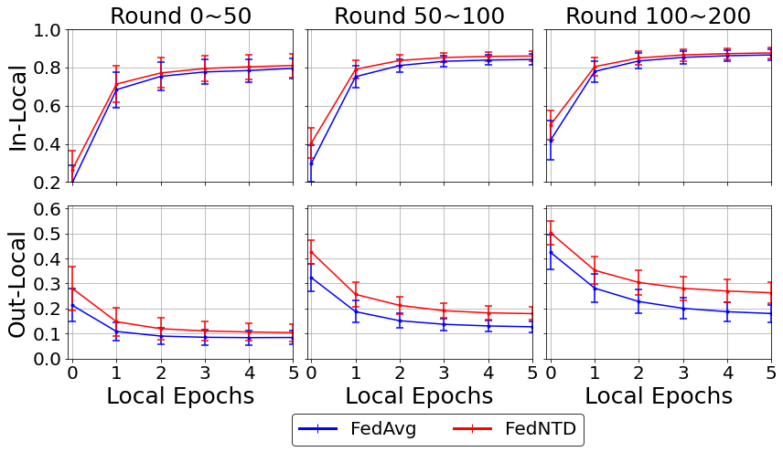
Figure 6: Accuracy on CIFAR-10 (s=2) in Local Training. The error bars stand for the standard deviation on clients.

In Figure 7, we present the test accuracy on diverse heterogeneity levels. Although both FedAvg and FedNTD show little change in local accuracy on in-local distribution $p(x)$, FedNTD significantly improves the local accuracy on out-local distribution $\tilde{p}(x)$, which implies it prevents forgetting. Along with it, the test accuracy of the global model also substantially improves. These gaps are enlarged when the number of local epochs increases, where the local models much deviate from the global model. The accuracy curves during local training are in Figure 6. It shows that fitting on the local distribution rapidly leads to forgetting on out-local distribution, But FedNTD effectively relieves this tendency without hurting the learning ability towards the in-local distribution.

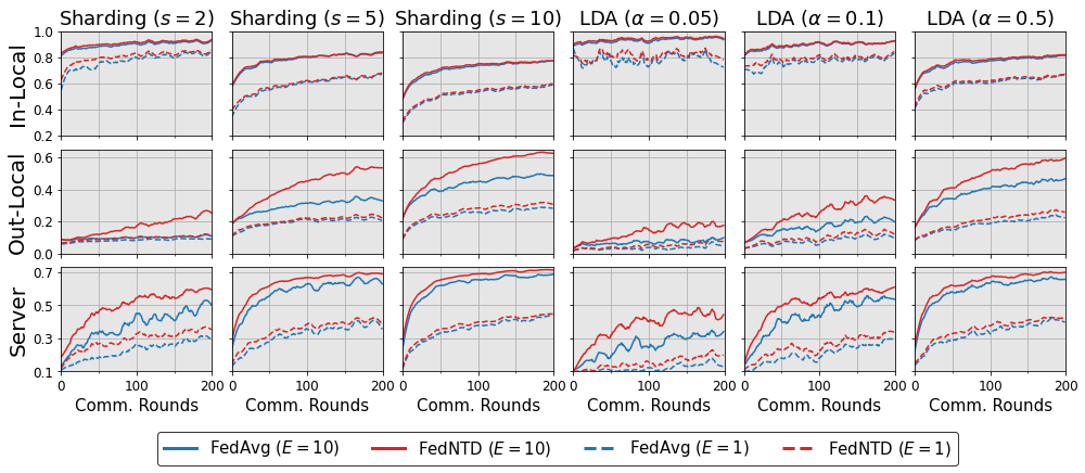
Figure 7: Learning curves of FedAvg [37] (blue line) and our FedNTD (red line) on CIFAR-10 with various heterogeneity setups for local epochs $E\in\{1,10\}$. ($\text{1}^{\text{st}}$ and $\text{2}^{\text{nd}}$ row) : Local test accuracy on in-local distribution $p(x)$ and out-local distribution $\tilde{p}(x)$. ($\text{3}^{\text{rd}}$ row): Global server test accuracy.

Our interest is how the FedNTD’s knowledge preservation on out-local distribution benefits on the federated learning, despite little change of its performance on in-local distribution. To figure it out, we analyze the local models in FedNTD after local training, and suggest two main reasons:

• Weight Alignment: How much the semantics of each weight is preserved?

• Weight Divergence: How far the local weights drift from the global model?

5.1 Weight Alignment

In recent studies, it has been suggested that there is a mismatch of semantic information encoded in the weight parameters across local models, even for the same coordinates (i.e., same position) [54, 46, 53]. As the current aggregation scheme averages weights of the identical coordinates, matching the semantic alignment across local models plays an important role in global convergence.

To analyze the semantic alignment of each parameter, we identify the individual neuron’s class preference by which class has the largest activation output on average. We then measure the alignment for a layer between two different models as the proportion of neurons that the class preference is matched for each other. The result is provided in Table 2.

While FedAvg and FedNTD show little difference in the IID case, FedNTD significantly enhances the alignment in the NIID cases. The visualized results are in Appendix M, with more details on how the alignment is measured. We further analyze the change of feature after local training using a unit hypersphere in Appendix N and T-SNE in Appendix O.

Table 2: Alignment of last two fc-layers for Distributed Global (DG), 10 Locals (L), and Aggregated Global (AG) models on CIFAR-10 datasets for IID and NIID (Sharding $s=2$, LDA $\alpha=0.05$) at round 200.

Layer	Alignment	IID		NIID ($s=2$)		NIID ($\alpha=0.05$)
		FedAvg	FedNTD	FedAvg	FedNTD	FedAvg	FedNTD
Linear_1 (dim: 512)	$W_{G}^{(t-1)}$ vs. $W_{L}^{(t)}$	0.679	0.668	0.635	0.703	0.597	0.756
	$W_{G}^{(t-1)}$ vs. $W_{G}^{(t)}$	0.850	0.830	0.787	0.871	0.670	0.856
Linear_1 (dim: 128)	$W_{G}^{(t-1)}$ vs. $W_{L}^{(t)}$	0.771	0.765	0.488	0.552	0.512	0.730
	$W_{G}^{(t-1)}$ vs. $W_{G}^{(t)}$	0.898	0.906	0.609	0.836	0.586	0.859

5.2 Weight Divergence

The knowledge preservation by FedNTD leads the global model to predict each class more evenly. Here we describe how the global model with even prediction performance stabilizes the weight divergence. Consider a model fitted on a specific original distribution, and now it is trained on a new distribution. Then the weight distance between the original model and fitted model increases as the distance between the original distribution and new distribution grows.

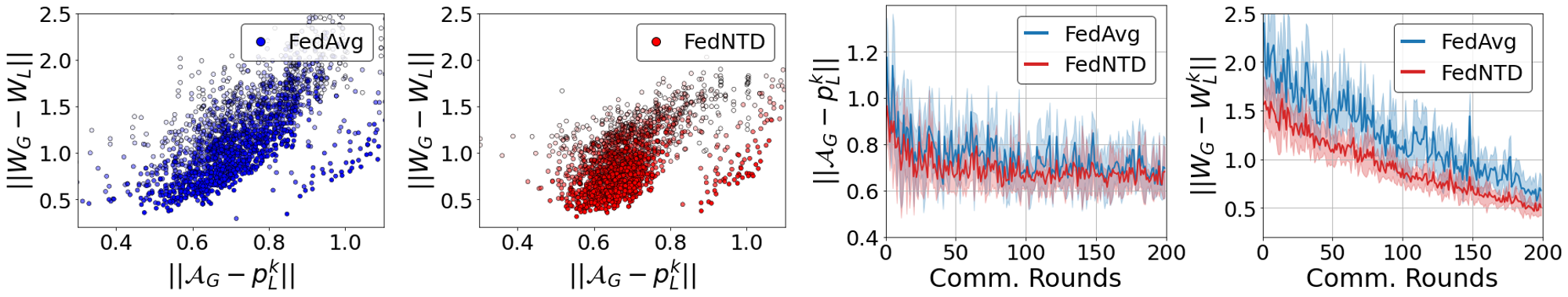
Figure 8: Distances for weights and distributions on CIFAR10 (s=2). (a), (b): The relationship between two distances. The opacity is higher for later rounds. (c), (d): The measured distances for 200 rounds.

We argue that if the distance between the global model’s underlying distribution and local distributions is small, the moved distance between the global model and local models also becomes close. If we assume the local distributions are generated arbitrarily, the most robust choice for the global model’s underlying distribution is a uniform distribution. We formally rephrase our argument as the follows:

Proposition 3.

Let $\mathbb{P}\mathrel{\mathop{\mathchar 58\relax}}\Delta_{\mathcal{C}}\rightarrow\mathbb{R}_{\geq 0}$ be the probability measure for the client’s local distribution and $\Pi$ be the set of measure in the hypothesis. Assume that the class-wise loss $\mathcal{L}_{c}(w)=\mathbb{E}_{x|y=c}[\mathcal{L}(x;w)]$ is $\lambda$-smooth and $w_{c}$ be a optimum of $\mathcal{L}_{c}$. Then the loss $\mathcal{L}$ of the client with distribution $p$ becomes:

$$\small\mathcal{L}(w)=\sum_{c}p_{c}\mathcal{L}_{c}(w)\leq\sum_{c}p_{c}\mathcal{L}_{c}(w_{c})+\frac{1}{2}\lambda\sum_{c}p_{c}\lVert w-w_{c}\rVert^{2}\,.$$ (15)

Then for arbitrary $\mathbb{P}\in\Pi$, the uniform distribution attains the minimax value:

$$\text{unif.dist}\in\underset{p\in\Delta_{\mathcal{C}}}{\textup{argmin}}\>\underset{\mathbb{P}\in\Pi}{\textup{sup}}\>\mathbb{E}_{p^{\prime}\sim\mathbb{P}}[\lVert w_{p^{\prime}}-w_{p}\rVert]\,,\>\>\textup{where}\>\>w_{p}=\sum_{c}p_{c}w_{c}\,.$$ (16)

The proof is provided in Appendix S. Although the global model’s underlying distribution is unknown, the normalized class-wise accuracy vector is a handy approximation for it as: $\mathcal{A_{\text{G}}}=\frac{1}{A}\cdot[a_{1},\dots a_{\mathcal{C}}]$, where $A$ is the global model’s test accuracy and $a_{c}$ is its class-wise accuracy on the class $c$.

The results in Figure 8 empirically validate our argument. There is a strong correlation between weight divergence $\|w-w_{k}\|$ (for global model $w$ and client $k$’s local model $w_{k}$) and distribution distance $\|\mathcal{A}_{G}-p_{k}\|$ (for client $k$’s distribution $p_{k}$). By providing a better starting point for local training, FedNTD effectively stabilizes the weight divergence.

6 Related Work

Federated Learning (FL)

is proposed to update a global model while the local data is kept in clients’ devices [24, 23]. The standard algorithm is FedAvg [37], which aggregates trained local models by averaging their parameters. Although its effectiveness has been largely discussed in i.i.d. settings [48, 44], many algorithms obtain the sub-optimal when the distributed data is heterogeneous [31, 56]. Until recently, a wide range of variants of FedAvg has been proposed to overcome such a problem. One line of work focuses on local-side modification by regularizing the deviation of local models from the global model [30, 20, 1, 47]. Another is the server-side modification, which improves the efficacy of aggregation of local models in the server [46, 33, 55, 9]. Our work aims to preserve global knowledge during local training, which belongs to the local-side approach.

Forgetting View in FL

A pioneer work that considers forgetting in FL is FedCurv [43]. It regards each local client as a task, and [43] regulates the change of local parameters to prevent accuracy drop on all other clients. However, it needs to compute and communicate parameter-wise importance across clients, which severely burdens the learning process. On the other hand, we focus on the class-wise forgetting and suggest that not-true logits from local data contain enough knowledge to prevent it. A concurrent work of our study is [49], which also reports the forgetting issue in local clients by empirically showing the increasing loss of previously learned data after the local training. To prevent forgetting, [49] exploits generated pseudo data. Instead, we focus on the class-wise forgetting and suggest that not-true logits from local data contain enough knowledge to prevent it. The continual learning literature is further discussed in Appendix D.

Knowledge Distillation (KD) in FL

In FL, a typical approach is using KD to make the global model learn from the ensemble of local models [9, 33, 26, 57]. By leveraging the unlabeled auxiliary data, KD effectively tackles the local drifts by enriching the aggregation. However, such carefully engineered proxy data and may not always be available [30, 58, 55]. Although more recent works generate pseudo-data to extract knowledge by data-free KD [58, 55], they require additional heavy computation, and the quality of samples is sensitive to the many hyperparameters involved in the process. On the other hand, as a simple variant of KD, our proposed method surprisingly performs well on heterogeneity scenarios without any additional resource requirements.

7 Conclusion

This study begins from an analogy to continual learning and suggests that forgetting could be a major concern in federated learning. Our observations show that the knowledge outside of local distribution is prone to be forgotten in local training and is closely related to the unstable global convergence. To overcome this issue, we propose a simple yet effective algorithm, FedNTD, which conducts local-side distillation only for the not-true classes to prevent forgetting. FedNTD does not have any additional requirements, unlike previous approaches. We analyze the effect of FedNTD from various perspectives and demonstrate its benefits in federated learning.

Broader Impact

We believe that Federated Learning is an important learning paradigm that enables privacy-preserving ML. Our work suggests the forgetting issue and introduces the methods to relive it without compromising data privacy. The insight behind this work may inspire new researches. However, the proposed method maintains the knowledge outside of local distribution in the global model. This implies that if the global model is biased, the trained local model is more prone to have a similar tendency. This should be considered for ML participators.

Checklist

The checklist follows the references. Please read the checklist guidelines carefully for information on how to answer these questions. For each question, change the default [TODO] to [Yes] , [No] , or [N/A] . You are strongly encouraged to include a justification to your answer, either by referencing the appropriate section of your paper or providing a brief inline description. For example:

• Did you include the license to the code and datasets? [Yes] The datasets are public datasets and the code is MIT license

Please do not modify the questions and only use the provided macros for your answers. Note that the Checklist section does not count towards the page limit. In your paper, please delete this instructions block and only keep the Checklist section heading above along with the questions/answers below.

1. For all authors…

   1. Do the main claims made in the abstract and introduction accurately reflect the paper’s contributions and scope? [Yes] We clarified the scope in both abstract and introduction. The contributions are summarized at the end of Section 1.

   2. Did you describe the limitations of your work? [Yes] Before reference, we discussed about potential limitations as broad impact

   3. Did you discuss any potential negative societal impacts of your work? [Yes] Before reference, we discussed as broader impact

   4. Have you read the ethics review guidelines and ensured that your paper conforms to them? [Yes]

2. If you are including theoretical results…

   1. Did you state the full set of assumptions of all theoretical results? [Yes] In all proposition parts. The detailed notations are in Appendix A.

   2. Did you include complete proofs of all theoretical results? [Yes] Included in the corresponding Appendix sections.

3. If you ran experiments…

   1. Did you include the code, data, and instructions needed to reproduce the main experimental results (either in the supplemental material or as a URL)? [Yes] Included in supplemental material

   2. Did you specify all the training details (e.g., data splits, hyperparameters, how they were chosen)? [Yes] Included in the Appendix.

   3. Did you report error bars (e.g., with respect to the random seed after running experiments multiple times)? [Yes] We indicated the standard deviation of each result for the main experiments in the corresponding Appendix section.

   4. Did you include the total amount of compute and the type of resources used (e.g., type of GPUs, internal cluster, or cloud provider)? [Yes] Included in the Appendix.

   1. If your work uses existing assets, did you cite the creators? [Yes]

   2. Did you mention the license of the assets? [Yes]

   3. Did you include any new assets either in the supplemental material or as a URL? [Yes]

   4. Did you discuss whether and how consent was obtained from people whose data you’re using/curating? [N/A] We used the public benchmarks.

   5. Did you discuss whether the data you are using/curating contains personally identifiable information or offensive content? [N/A] We only used the public dataset that has been sufficiently considered about the issues.

4. If you used crowdsourcing or conducted research with human subjects…

   1. Did you include the full text of instructions given to participants and screenshots, if applicable? [N/A]

   2. Did you describe any potential participant risks, with links to Institutional Review Board (IRB) approvals, if applicable? [N/A]

   3. Did you include the estimated hourly wage paid to participants and the total amount spent on participant compensation? [N/A]

Appendix A Table of Notations

Table 3: Table of Notations throughout the paper.

Indices:
$c\,,c^{\prime}$	index for classes ($c\in\{1,...,\mathcal{C}\}=[\mathcal{C}]$)
$i$	index for data ($i\in\{1,...,N\}=[N]$)
$k\,,k^{\prime}$	index for clients ($k\in\{1,...,K\}=[K]\text{ or }\in K^{(t)}$)
$t$	index for rounds ($t\in\{1,...,\mathcal{T}\}=[\mathcal{T}]$)
$e$	index for local epochs ($t\in\{1,...,E\}=[E]$)
Parameters:
$\alpha$	Parameter for the Dirichlet Distribution
$s$	The Number of shards per user
$\beta$	Hyperparameter for the distillation loss; generally controls the relative weight of divergence loss
$\tau$	The temperature on the softmax
$\gamma$	Learning rate
Data and Weights:
$\mathcal{D}$	whole dataset
$\mathcal{D}^{k}$	local dataset
$x$	datum
$y$	class label for datum
$w^{(t)}$	weight of the server model on the round $t$
$w_{k}^{(t)}$	weight of the $k$-th client model on the round $t$
$\|W_{G}-W_{L}\|$	Collection of $L^{1}$-norm between server and client models, among all rounds.
Softmax Probabilities:
$q_{\mathcal{\tau}}^{T}\,/\,q_{\mathcal{\tau}}^{S}$	The softened softmax probability of teacher/student model
$q^{g}\,/\,q^{l}$	The softmax probability on the server/client model
${\tilde{q}_{\tau}}^{g}\,/\,{\tilde{q}_{\tau}^{l}}$	The softened softmax probability calculated without true-class logit on the server/client model
Class Distribution on Datasets:
$p=[p_{1}\,,\ldots,p_{\mathcal{C}}]$	In-local distribution of dataset
$\tilde{p}=[\tilde{p}_{1}\,,\ldots,\tilde{p}_{\mathcal{C}}]$	Out-local distribution of dataset
Loss Functions:
$\mathcal{L}_{\textup{CE}}$	cross-entropy loss
$\mathcal{L}_{\textup{KL}}$	Kullback-Leibler divergence
$\mathcal{L}_{\textup{NTD}}$	Proposed Not-True Distillation Loss
Accuracy and Forgetting Measure:
$\mathcal{A}_{c}^{(t)}$	Accuracy of the server model on the $c$-th class, at round $t$.
$\|\mathcal{A}_{G}-p_{L}^{k}\|$	Collection of $L^{1}$-norm between normalized global accuracy and data distribution on each client, among all rounds.
$\mathcal{F}$	Backward Transfer (BwT). For the federated learning situation, we calculate this measure on the server model.

Appendix B Experimental Setups

Here we provide details of our experimental setups. The code is implemented by PyTorch [41] and the overall code structure is based on FedML [16] library with some modifications. We use 1 Titan-RTX and 1 RTX 2080Ti GPU card. Multi-GPU training is not conducted in the paper experiments.

B.1 Model Architecture

The model architecture used in our experiment is from [37], which is composed of two convolutional layers followed by max-pooling layers, and two fully connected layer. A similar architecture is used in [28, 34].

B.2 Datasets

We mainly used four benchmarks: MNIST [11], CIFAR-10 [25], CIFAR-100 [25], and CINIC-10 [10]. The details about each datasets and setups are described in Table 4. We augment the training data using Random Cropping, Horizontal Flipping, and Normalization. For MNIST, CIFAR-10, and CIFAR-100, we add Cutout [12] augmentation.

Table 4: Details datasets setups used in the experiment.

Datasets	MNIST	CIFAR-10	CIFAR-100	CINIC-10
Datasets Classes	10	10	100	10
Datasets Size	50,000	50,000	50,000	90,000
Number of Clients	100	100	100	200
Client Sampling Ratio	0.1	0.1	0.1	0.05
Local Epochs (E)	3	5	5	5
Batch Size (B)	50	50	50	50

B.3 Learning Setups

We use a momentum SGD optimizer with an initial learning rate of 0.01, and the momentum is set as 0.9. The momentum is only used in the local training, which implies the momentum information is not communicated to the server. The learning rate is decayed with a factor of 0.99 at each round, and a weight decay of 0.00001 is applied. In the motivational experiment in Section 3, we fix the learning rate as 0.01. Since we assume a synchronized federated learning scenario, parallel distributed learning is simulated by sequentially training the sampled clients and then aggregating them as a global model.

B.4 Algorithm Implementation Details

For the implemented algorithms, we search hyperparameters and choose the best among the candidates. The hyperparameters for each algorithm is in Table 5.

Table 5: Algorithm-specific hyperparameters used in the experiment.

Method	Hyperparameters	Searched Candidates
FedAvg [37]	None	None
FedCurv [43]	$s=500$, $\lambda=1.0$	$s\in\{250,500\}$, $\lambda\in\{0.1,0.5,1.0\}$
FedProx [30]	$\mu=0.1$	$\mu\in\{0.1,0.5,1.0\}$
FedNova [47]	None	None
SCAFFOLD [20]	None	None
MOON [28]	$\mu=1.0$, $\tau=0.5$	$\mu\in\{0.1,0.5,1.0\}$, $\tau\in\{0.1,0.5,1,0\}$
FedNTD (Ours)	$\beta$=1.0, $\tau=1.0$	None

B.5 Non-IID Partition Strategy

To widely address the heterogeneous federated learning scenarios, we distribute the data to the local clients with the following two strategies: (1) Sharding and (2) Latent Dirichlet Allocation (LDA).

Sharding

In the Sharding strategy, we sort the data by label and divide it into the same-sized shards without overlapping. In detail, a shard contains $\frac{|D|}{N\times s}$ size of same class samples, where $D$ is the total dataset size, $N$ is the total number of clients, and $s$ is the number of shards per user. Then, we distribute s number of shards to each client. $s$ controls the heterogeneity of local data distribution. The heterogeneity level increases as the shard per user $s$ becomes smaller and vice versa. Note that we only test the statistical heterogeneity (skewness of class distribution across the local clients) in the Sharding strategy, and the size of local datasets is identical.

Latent Dirichlet Allocation (LDA)

In LDA strategy, Each client $k$ is allocated with $p_{c,k}$ proportion of the training samples of class $c$, where $p_{c}\sim\text{Dir}_{K}(\alpha)$ and $\alpha$ is the concentration parameter controlling the heterogeneity. The heterogeneity level increases as the concentration parameter $\alpha$ becomes smaller, and vice versa. Note that both the class distribution and local datasets sizes differ across the local clients in LDA strategy.

Appendix C Conceptual comparison to prior works

The conceptual illustration of federated distillation methods is in Figure 9. The existing algorithms either use additional local information (9(a)) or need an auxiliary (or proxy) data to conduct distillation. On the other hand, our proposed FedNTD does not have such constraints (9(c)).

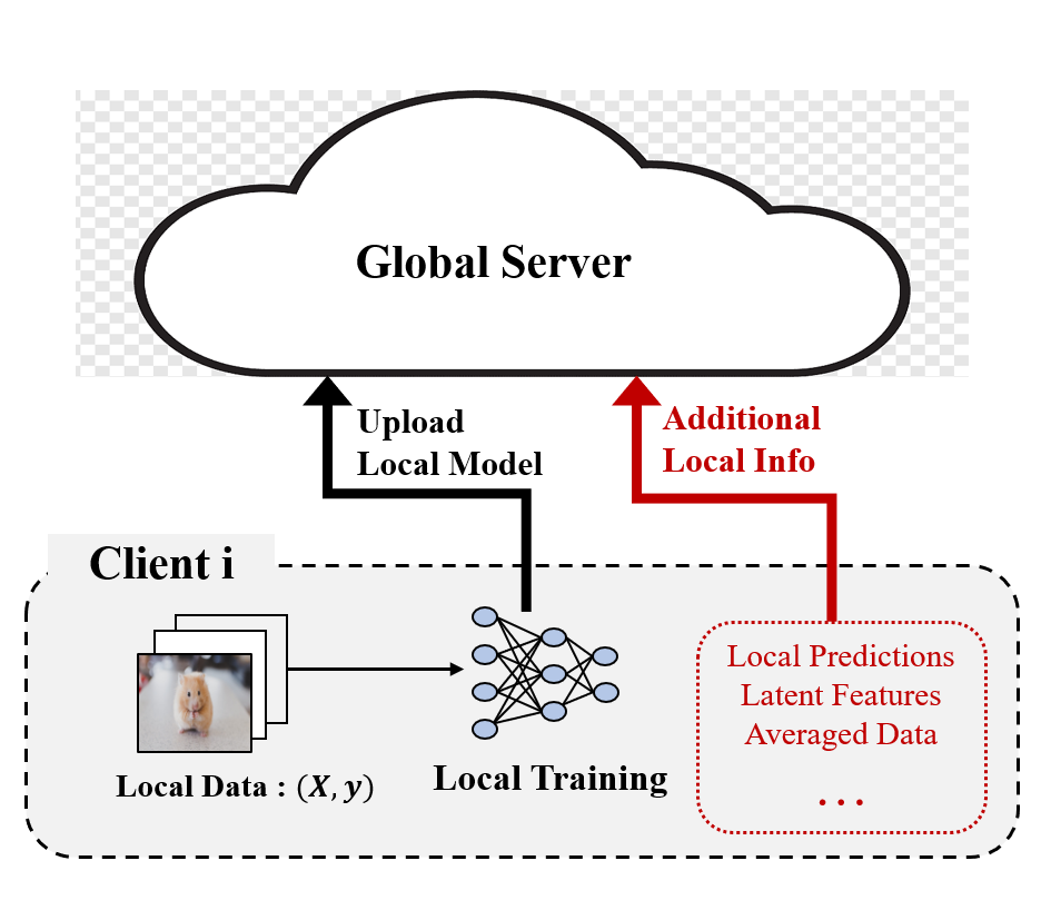
(a) Use Additional Local Info

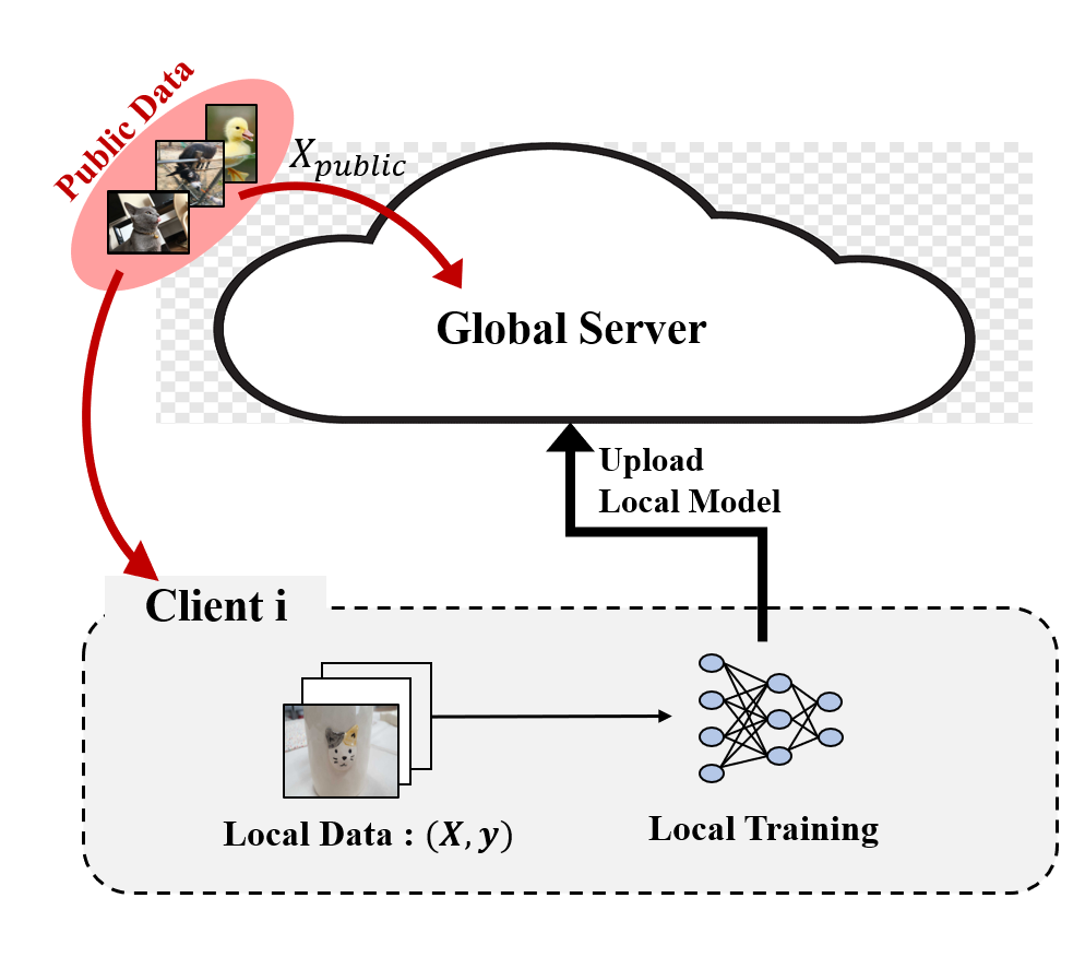
(b) Use Auxiliary Datasets

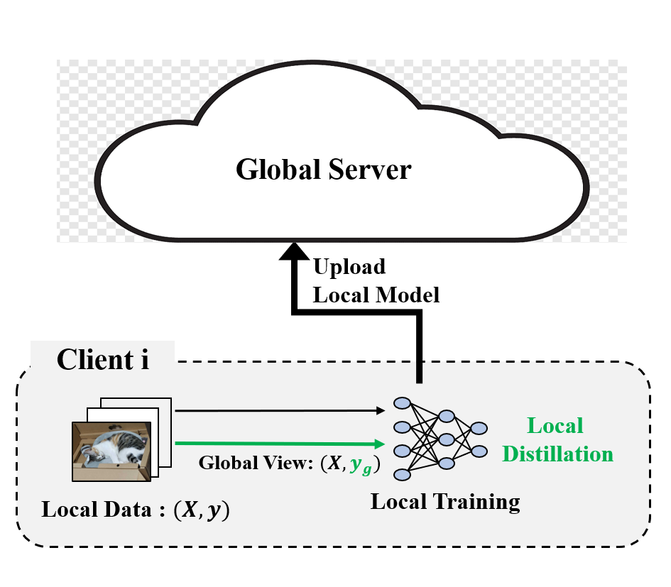
(c) FedNTD (ours)

Figure 9: An overview of federated distillation methods.

Table 6: Additional resource requirements compared to FedAvg.

Method	No Additional Requirements on:
	Statefulness?	Communication Cost?	Auxiliary Data?
FedEnsemble [33]	✔	✔	✕
FedBE [9]	✔	✕	✕
MOON [28]	✕	✔	✔
SCAFFOLD [20]	✕	✕	✔
FedNTD (Ours)	✔	✔	✔

Appendix D Related Work: Continual Learning

Continual Learning (CL) is a learning paradigm that updates a sequence of tasks instead of training on the whole datasets at once [42, 45]. In CL, the main challenge is to avoid catastrophic forgetting [15], whereby training on the new task interferes with the previous tasks. Existing methods try to mitigate this problem by various strategies. In Parameter-based approaches, the importance of parameters for the previous task is measured to restrict their changes [5, 22, 3]. Regularization-based approaches [4, 32] introduce regularization terms to prevent forgetting. Memory-based approaches [8, 6] keep a small episodic memory from the previous tasks and replay it to maintain knowledge. Our work is more related to the regularization-based approaches, introducing the additional local objective term to prevent forgetting out-local knowledge.

It would be worth to mention that there are some works that tried to conduct classical continual learning problems in federated learning setups. For example, [51] studied the scenario in which each local client has to learn a sequence of tasks. Here, the task-specific parameters are decomposed from the global parameters to minimize the interference between tasks. In [13], the relation knowledge for the old classes is transferred round by round with class-aware gradient compensations.

Appendix E Server Prediction Consistency

We extend the motivational experiment in Section 3.1 to the main experimental setups. Here, we plotted the normalized class-wise test accuracy for each case to identify the contribution of each class on the current accuracy. This helps observe the prediction consistency regardless of the highly fluctuating global server accuracy in the non-IID case. As in Figure 10, FedNTD effectively preserves the knowledge from the previous rounds; thereby the global server model becomes to predict each class evenly much earlier than FedAvg. Note that we normalize the class-wise test accuracy as round-by-round manner, which makes the sum for each round as 1.0.

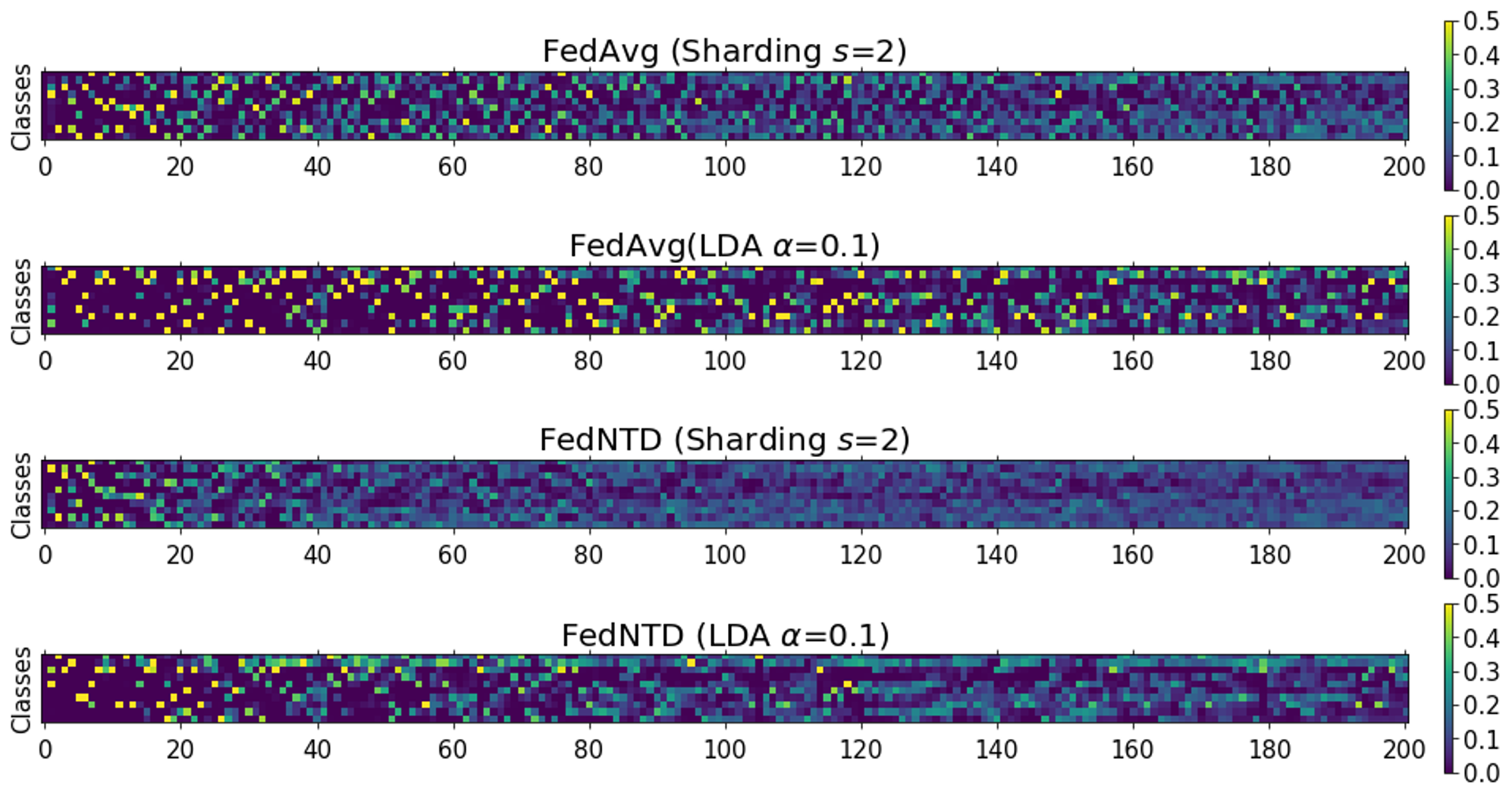
Figure 10: Visualized server test accuracy of FedAvg and FedNTD on CIFAR-10 datasets.

Appendix F Experiment Table with Standard Deviation

Table 7: Accuracy@1 (%) on MNIST [11], CIFAR-10 [25], CIFAR-100 [25], and CINIC-10 [10]. The values in the parenthesis are the standard deviation. The arrow ($\downarrow$,  $\uparrow$)  shows the comparison to the FedAvg.

NIID Partition Strategy : Sharding
Method	MNIST	CIFAR-10				CIFAR-100	CINIC-10
		$s=2$	$s=3$	$s=5$	$s=10$
FedAvg [37]	78.63${}_{\pm 0.42}\;\;$	40.14${}_{\pm 1.15}\;\;$	51.10${}_{\pm 0.11}\;\;$	57.17${}_{\pm 0.12}\;\;$	64.91${}_{\pm 0.69}\;\;$	25.57${}_{\pm 0.44}\;\;$	39.64${}_{\pm 0.78}\;\;$
FedCurv [43]	78.56±0.23 $\downarrow$	44.52±0.44 $\uparrow$	49.00±0.41 $\downarrow$	54.61±0.20 $\downarrow$	62.19±0.47 $\downarrow$	22.89±0.66 $\downarrow$	40.45±0.25 $\uparrow$
FedProx [30]	78.26±0.28 $\downarrow$	41.48±1.08 $\uparrow$	51.65±0.53 $\uparrow$	56.88±0.15 $\downarrow$	64.65±0.61 $\downarrow$	25.10±0.67 $\downarrow$	41.47±0.99 $\uparrow$
FedNova [47]	77.04±0.98 $\downarrow$	42.62±1.32 $\uparrow$	52.03±1.49 $\uparrow$	62.14±0.74 $\uparrow$	66.97±0.39 $\uparrow$	26.96±0.59 $\uparrow$	42.55±0.10 $\uparrow$
SCAFFOLD [20]	81.05±0.26 $\uparrow$	44.60±2.24 $\uparrow$	54.26±0.22 $\uparrow$	65.74±0.36 $\uparrow$	68.97±0.34 $\uparrow$	30.82±0.31 $\uparrow$	42.66±0.92 $\uparrow$
MOON [28]	76.56±0.24 $\downarrow$	38.51±0.96 $\downarrow$	50.47±0.15 $\downarrow$	56.69±0.11 $\downarrow$	65.30±0.51 $\uparrow$	25.29±0.24 $\downarrow$	37.07±0.24 $\downarrow$
FedNTD (Ours)	84.44±0.43 $\uparrow$	52.61±1.00 $\uparrow$	58.18±1.42 $\uparrow$	64.93±0.34 $\uparrow$	68.56±0.24 $\uparrow$	31.69±0.13 $\uparrow$	48.07±0.36 $\uparrow$
NIID Partition Strategy : LDA
Method	MNIST	CIFAR-10				CIFAR-100	CINIC-10
		$\alpha=0.05$	$\alpha=0.1$	$\alpha=0.3$	$\alpha=0.5$
FedAvg [37]	79.73${}_{\pm 0.20}\;\;$	28.24${}_{\pm 3.11}\;\;$	46.49${}_{\pm 0.93}\;\;$	57.24${}_{\pm 0.21}\;\;$	62.53${}_{\pm 0.41}\;\;$	30.69${}_{\pm 0.27}\;\;$	38.14${}_{\pm 3.40}\;\;$
FedCurv [43]	78.72±0.44 $\downarrow$	33.64±2.98 $\uparrow$	44.26±0.79 $\downarrow$	54.93±0.46 $\downarrow$	59.37±0.24 $\downarrow$	29.16±0.22 $\downarrow$	36.69±3.03 $\downarrow$
FedProx [30]	79.25±0.16 $\downarrow$	37.19±3.17 $\uparrow$	47.65±0.90 $\uparrow$	57.35±0.40 $\uparrow$	62.39±0.31 $\downarrow$	30.60±0.16 $\downarrow$	39.47±3.40 $\uparrow$
FedNova [47]	60.37±2.71 $\downarrow$	10.00 (Failed) $\downarrow$	28.06±0.12 $\downarrow$	57.44±1.69 $\uparrow$	64.65±0.34 $\uparrow$	32.15±0.13 $\uparrow$	30.44±1.35 $\downarrow$
SCAFFOLD [20]	71.57±0.72 $\downarrow$	10.00 (Failed) $\downarrow$	23.12±0.55 $\downarrow$	62.01±0.34 $\uparrow$	66.16±0.13 $\uparrow$	33.68±0.13 $\uparrow$	28.78±1.26 $\downarrow$
MOON [28]	78.95±0.46 $\downarrow$	28.35±3.68 $\uparrow$	44.77±1.12 $\downarrow$	58.38±0.09 $\uparrow$	63.10±0.00 $\uparrow$	30.64±0.12 $\downarrow$	37.92±3.31 $\downarrow$
FedNTD (Ours)	81.34±0.33 $\uparrow$	40.17±3.19 $\uparrow$	54.42±0.06 $\uparrow$	62.42±0.53 $\uparrow$	66.12±0.26 $\uparrow$	32.37±0.02 $\uparrow$	46.24±1.67 $\uparrow$

Appendix G Additional Experiments

G.1 Effect of Local Epochs

Table 8: Accuracy@1 on CIFAR-10 (Sharding $s=2$). The value in the parenthesis is the forgetting $\mathcal{F}$.

NIID Partition Strategy: Sharding ($s=2$)
Method	Local Epochs (E)
	1	3	5	10	20
FedAvg [37]	29.49 (0.70)	34.49 (0.64)	40.14 (0.59)	50.08 (0.49)	56.93 (0.42)
FedProx [30]	29.44 (0.69) $\downarrow$	34.00 (0.64) $\downarrow$	41.48 (0.57) $\uparrow$	42.74 (0.53) $\downarrow$	43.39 (0.52) $\downarrow$
FedNova [47]	27.77 (0.71) $\downarrow$	32.00 (0.64) $\downarrow$	42.62 (0.56) $\uparrow$	48.59 (0.50) $\downarrow$	58.24 (0.39) $\uparrow$
SCAFFOLD [20]	34.46 (0.64) $\uparrow$	39.26 (0.58) $\uparrow$	44.60 (0.53) $\uparrow$	55.35 (0.41) $\uparrow$	62.80 (0.34) $\uparrow$
FedNTD (Ours)	35.77 (0.64) $\uparrow$	45.47 (0.50) $\uparrow$	52.61 (0.43) $\uparrow$	60.22 (0.36) $\uparrow$	60.61 (0.34) $\uparrow$

Table 9: Accuracy@1 on CIFAR-10 (LDA $\alpha=0.1$). The value in the parenthesis is the forgetting $\mathcal{F}$.

NIID Partition Strategy: LDA ($\alpha=0.1$)
Method	Local Epochs (E)
	1	3	5	10	20
FedAvg [37]	29.77 (0.69)	37.70 (0.60)	46.49 (0.51)	53.80 (0.43)	57.70 (0.39)
FedProx [30]	33.37 (0.65) $\uparrow$	37.88 (0.57) $\uparrow$	47.65 (0.49) $\uparrow$	44.02 (0.50) $\downarrow$	44.98 (0.49) $\downarrow$
FedNova [47]	26.35 (0.73) $\downarrow$	24.37 (0.74) $\downarrow$	28.06 (0.71) $\downarrow$	47.41 (0.50) $\downarrow$	10.00 (Failure) $\downarrow$
SCAFFOLD [20]	13.36 (0.86) $\downarrow$	22.04 (0.75) $\downarrow$	23.12 (0.74) $\downarrow$	38.49 (0.57)$\downarrow$	47.07 (0.47) $\downarrow$
FedNTD (Ours)	33.94 (0.64) $\uparrow$	45.92 (0.50) $\uparrow$	54.42 (0.42) $\uparrow$	60.67 (0.33) $\uparrow$	62.25 (0.30) $\uparrow$

G.2 Effect of Sampling Ratio

Table 10: Accuracy@1 on CIFAR-10 (Sharding $s=2$). The value in the parenthesis is the forgetting $\mathcal{F}$.

NIID Partition Strategy: Sharding ($s=2$)
Method	Client Sampling Ratio (R)
	0.05	0.1	0.3	0.5	1.0
FedAvg [37]	33.06 (0.66)	40.14 (0.59)	49.99 (0.46)	52.98 (0.41)	51.48 (0.30)
FedProx [30]	35.36 (0.63) $\uparrow$	41.48 (0.57) $\uparrow$	44.54 (0.45) $\downarrow$	50.02 (0.31) $\downarrow$	52.53 (0.06) $\uparrow$
FedNova [47]	29.99 (0.69) $\downarrow$	42.62 (0.56) $\uparrow$	55.59 (0.31) $\uparrow$	56.75 (0.23) $\uparrow$	51.89 (0.34) $\uparrow$
SCAFFOLD [20]	29.15 (0.70) $\downarrow$	44.60 (0.53) $\uparrow$	55.59 (0.31) $\uparrow$	56.75 (0.23) $\uparrow$	57.88 (0.10) $\uparrow$
FedNTD (Ours)	46.99 (0.51) $\uparrow$	52.61 (0.43) $\uparrow$	59.37 (0.28) $\uparrow$	60.70 (0.18) $\uparrow$	61.53 (0.04) $\uparrow$

Table 11: Accuracy@1 on CIFAR-10 (LDA $\alpha=0.1$). The value in the parenthesis is the forgetting $\mathcal{F}$.

NIID Partition Strategy: LDA ($\alpha=0.1$)
Method	Client Sampling Ratio (R)
	0.05	0.1	0.3	0.5	1.0
FedAvg [37]	29.35 (0.70)	46.49 (0.51)	53.73 (0.39)	58.72 (0.25)	61.38 (0.04)
FedProx [30]	36.36 (0.63) $\uparrow$	47.65 (0.49) $\uparrow$	45.78 (0.37) $\downarrow$	49.65 (0.23) $\downarrow$	51.31 (0.07)) $\downarrow$
FedNova [47]	21.31 (0.78) $\downarrow$	28.06 (0.71) $\downarrow$	45.83 (0.49) $\downarrow$	55.09 (0.50) $\downarrow$	56.79 (0.30) $\downarrow$
SCAFFOLD [20]	15.80 (0.84) $\downarrow$	23.12 (0.74) $\downarrow$	41.29 (0.51) $\downarrow$	10.00 (Failure)$\downarrow$	10.00 (Failure)$\downarrow$
FedNTD (Ours)	45.80 (0.53) $\uparrow$	54.42 (0.42) $\uparrow$	58.57 (0.33) $\uparrow$	60.88 (0.19) $\uparrow$	62.48 (0.06) $\uparrow$

G.3 Results on ResNet-10 Model

We report an additional experiment on popular architecture, ResNet-10. The number of parameters in ResNet-10 is about 10x larger than the 2-conv + 2-fc model for the main experiments.

	FedAvg	Scaffold	MOON	FedNTD (ours)
Shard (s = 2)	36.01	44.59	35.21	46.27
Shard (s = 5)	39.21	65.08	51.02	65.92
LDA ($\alpha$ = 0.1)	33.35	38.78	33.57	49.85

Appendix H Comparison to KD

We analyze the advantage of FedNTD over KD by observing the performance of the loss function below. Note that $L(\lambda)$ moves from $\mathcal{L}_{\text{KD}}$ to $\mathcal{L}_{\text{NTD}}$ as $\lambda$ increases, and collapses to $\mathcal{L}_{\text{KD}}$ at $\lambda=0$ and $\mathcal{L}_{\text{NTD}}$ at and $\lambda=1$.

$$\mathcal{L}_{\scriptscriptstyle\text{KD}\rightarrow\text{NTD}}=\mathcal{L}_{\text{CE}}(q,\;\mathds{1}_{y})+L(\lambda),$$ (17)

$$L(\lambda)=(1-\lambda)\cdot\mathcal{L}_{\text{KD}}(q_{\tau}^{l},\;q_{\tau}^{g})+\lambda\cdot\mathcal{L}_{\text{NTD}}({\tilde{q}_{\tau}^{l}},\;{\tilde{q}_{\tau}^{g}}).$$ (18)

The result is in Table 12, which shows reaching $L(\lambda)$ to $\mathcal{L}_{NTD}$ significantly improves the performance. This improvement supports the effect of decoupling the not-true classes and the true classes: preservation of out-local distribution knowledge using not-true class signals and acquisition of new knowledge on true classes from local datasets.

Table 12: CIFAR-10 test accuracy by varying $\lambda$.

Partition Method	KD	KD $\rightarrow$ NTD					NTD
		0.1	0.3	0.5	0.7	0.9
Sharding ($s=2$)	46.2	46.4	46.9	47.6	48.8	50.2	52.6
LDA ($\alpha=0.1$)	50.8	50.9	51.4	51.9	52.6	53.6	54.9

To further analyze the effect of NTD, we measure the performance of the local model as the communication rounds proceed. The result is plotted in Figure 11. Note that the Personalized performance is evaluated on the test samples with the same label distribution of the local clients.

The result shows that although the KD considerably improves the server model performance, the local model learned by KD shows much lower local performance. On the other hand, FedNTD shows much higher local performance, which implies that NTD successfully tackles the distillation not to hinder the local learning.

We insist that such significant improvement by discarding true-class logits in the distillation loss comes from the better trade-off between attaining new knowledge from local data and preserving old knowledge in the global model, as suggested in Section 3.

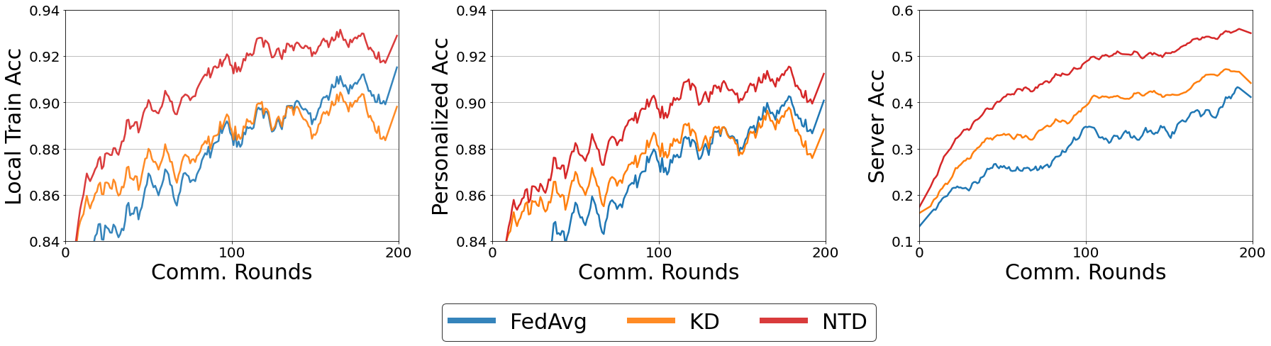
Figure 11: CIFAR-10 (Sharding: $s=2$) performances from KD and NTD

Appendix I Personalized performance of FL methods

Here we investigate the personalized performance of our FedNTD. As suggested in Appendix H, although FedNTD aims to improve global convergence, it also improves personalized performance. However, as the learning curves of SCAFFOLD (the green line) show, the lower local learning performance does not always lead to the worse server model performance. In all cases, SCAFFOLD shows significantly lower local performance at each round (the 1st and 2nd row), but it considerably improves the global convergence (the 3rd row).

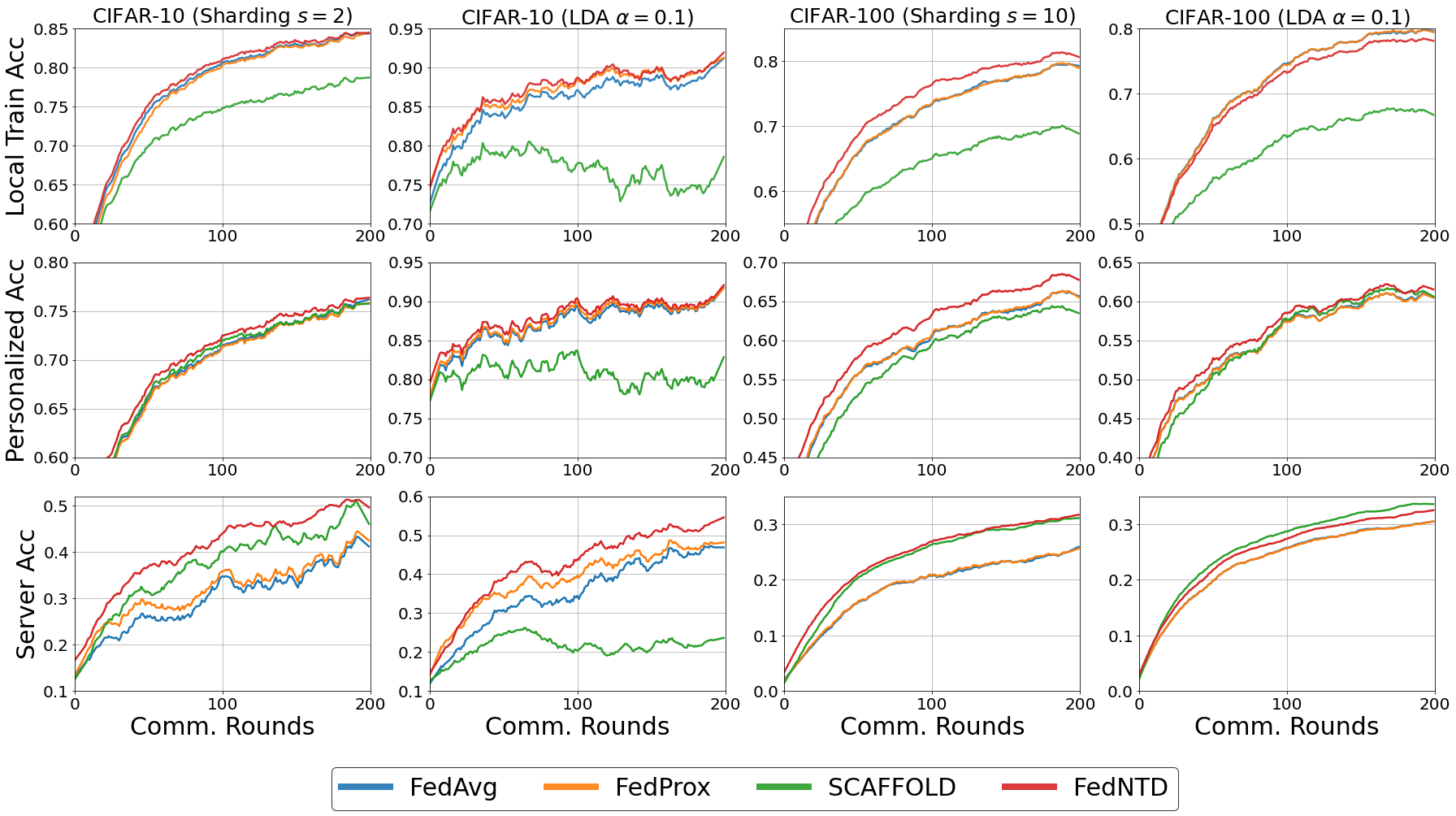
Figure 12: Local and global learning curves of FL methods. The accuracy of the local model is evaluated on: (Local Train) - the local private trains samples, and (Personalized): the test samples from the same label distribution with the local client

Appendix J Comparison to FedAlign

Here we compare our FedNTD with a recently proposed method, FedAlign [38], which shares the motivation of our work that local learning is the bottleneck of FL performance. In FedAlign, a correction term is introduced in the local learning target to obtain local models that generalize well. We implemented our FedNTD on officially released FedAlign code , and used the hyperparameters specified in [38]. The results are in Table 13 and Figure 13 shows their corresponding learning curves. In our experiment, although FedAlign improves the performance at some settings (LDA $\alpha=0.5$), its learning suffers when the heterogeneity level becomes severe. On the other hand, FedNTD consistently improves the performance even in such cases.

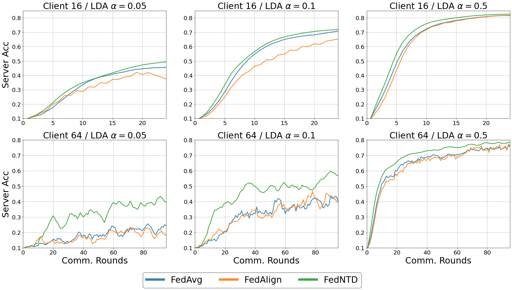
Figure 13: Learning curves that corresponds to Table 13.

Table 13: CIFAR-10 test accuracy. 16 clients participates for each communication round. The number local epochs is 20 for all experiments.

Client Number (LDA $\alpha$)	FedAvg [37]	FedAlign[38]	FedNTD (ours)
Client 16 ($\alpha=0.05$)	0.4556	0.3743	0.4943
Client 16 ($\alpha=0.1$)	0.7083	0.6532	0.7195
Client 16 ($\alpha=0.5$)	0.8163	0.8185	0.8266
Client 64 ($\alpha=0.05$)	0.2535	0.1854	0.3927
Client 64 ($\alpha=0.1$)	0.4247	0.3931	0.5634
Client 64 ($\alpha=0.5$)	0.7568	0.7698	0.7846

The introduced loss term of FedAlign aims to seek out-of-distribution generality w.r.t. global distribution during local training, resulting in the smooth loss landscape across domains (= heterogeneous local distributions in FL context). In Figure 14, we analyze the loss landscape using the parameter perturbation with Gaussian noise and the visualization using top-2 eigenvector axis, as in [38]. Interestingly, our FedNTD also smoothed the local landscape, implying that the local training does not require significant parameter change to fit its local distribution. We expect that one can get insight into the intriguing property in the loss space geometry to tackle the data heterogeneity problem for future work.

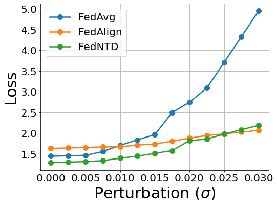
(a) Loss change by perturbation

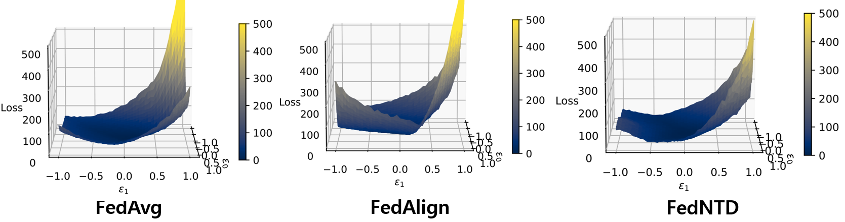
(b) Visualized loss landscape with Hessian eigenvectors $\epsilon_{0}$ and $\epsilon_{1}$.

Figure 14: Loss space of learned model (Client 16 / LDA $\alpha=0.5$).

Appendix K Effect of FedNTD Hyperparameters

In Figure 15, we plot the effect of FedNTD hyperparameters on the performance. The result shows that although FedNTD is not much sensitive to the choice of $\beta$, too small $\tau$ significantly drops the accuracy., which may be due to the too stiff not-true probability targets. The effect of both hyperparameters on the forgetting measure $\mathcal{F}$ is in Figure 16.

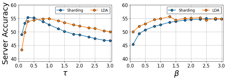
Figure 15: CIFAR-10 (Sharding: $s=2$, LDA: $\alpha=0.1$) test accuracy by varying FedNTD hyperparameter $\tau$ and $\beta$ values.

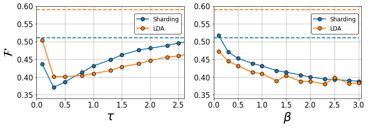
Figure 16: Forgetting $\mathcal{F}$ of FedNTD on CIFAR-10 by varying hyperparameters. The dotted lines stands for the baseline FedAvg.

Appendix L MSE Loss for Not-True Distillation

We explore how the MSE loss on Not-True Distillation acts. In Table 14, the MSE version FedNTD (FedNTD (MSE)) shows better accuracy and less forgets as $\beta$ grows, but at some degree, the model diverges; thereby cannot reach the original FedNTD, which exploits softmax and KL-Divergence loss to distill the knowledge in the global model. We explain it as matching all not-true logits using MSE logits is too strict to learn the global knowledge since the dark knowledge is mainly contained in top-k logits. FedNTD controls the class signals by using temperature-softened softmax.

Table 14: CIFAR-10 (Sharding s=2) results by varying $\beta$ for FedNTD (MSE) and FedNTD

Method	FedAvg	FedNTD (MSE)						FedNTD
$\beta$	0.0	0.001	0.005	0.01	0.05	0.1	0.3	1.0
Accuracy	40.14	40.53	42.39	43.02	44.41	44.27	Failure	52.61
Forgetting $\mathcal{F}$	0.59	0.58	0.56	0.55	0.53	0.53	Failure	0.43

Appendix M Visualization of Feature Alignment

To analyze feature alignment, we regard a neuron as the basic feature unit and identify individual neuron’s class preference as follows:

$$\mathcal{H}=[h_{1},h_{2}\dots h_{\mathcal{C}}],\>\>\text{where}\>\>{h}_{c}=\sum_{i=1}^{N_{c}}\mathcal{O}(x_{c,i}).$$ (19)

Here, the $\mathcal{O}(x_{c,i})$ denotes the neuron’s activation on data $x_{i}$ of class $c$, and $N_{c}$ is the number of samples for class $c$. For each neuron, we obtain the largest class index $\text{argmax}_{i}(\mathcal{H}_{i})$, to identify the most dominantly encoded class semantics. A similar measure is adopted in [53]. In Figure 17, we visualize the last layer neurons’ class preference. In both IID and NIID (Sharding $s=2$) cases, the features are more well-aligned in FedNTD.

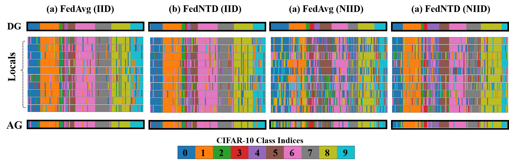
Figure 17: Visualized server test accuracy of FedAvg and FedNTD on CIFAR-10 (Sharding=2).

Appendix N Local features visualization: Hypersphere

To figure out forgetting of knowledge in the global model, we now analyze how the representation on the global distribution changes during local training. To this end, we design a straightforward experiment that shows the change of features on the unit hypersphere. More specifically, we modified the network architecture to map CIFAR-10 (Sharding $s=2$) input data to 2-dimensional vectors and normalize them to be aligned on the unit hypersphere $S^{1}=\{x\in\mathbb{R}^{2}\mathrel{\mathop{\mathchar 58\relax}}{||x||}_{2}=1\}$. We then estimate their probability density function. The global model is learned for 100 rounds of communication on homogeneous locals (i.i.d. distributed) and distributed to heterogeneous locals with different local distributions. The result is in Figure 18

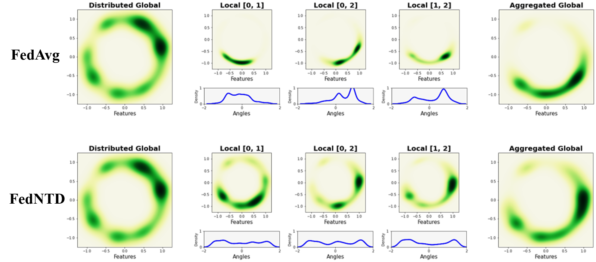
Figure 18: Features of CIFAR-10 (Sharding $s=2$) test samples on $S^{2}$. We plot the feature distribution with Gaussian kernel density estimation (KDE) in $\mathbb{R}^{2}$ and $\arctan(y,x)$ for each point $(x,y)\in S^{1}$. The distributed global model (first column) is trained on heterogeneous locals (middle 3 columns) and aggregated by parameter averaging (last column).

Appendix O Local features visualization: T-SNE

We further conduct an additional experiment on features of the trained local model. we trained the global server model for 100 communication rounds on heterogeneous (NIID) locals and distributed over 10 homogeneous (IID) locals and 10 heterogeneous (NIID) locals. In the homogeneous local case (19(a), 20(a)), the features are clustered by classes, regardless of which local they are learned from. On the other hand, in the heterogeneous local case (19(b), 20(b)), the features are clustered by which local distribution is learned. In Figure 21, we visualize the effect of FedNTD on the local features.

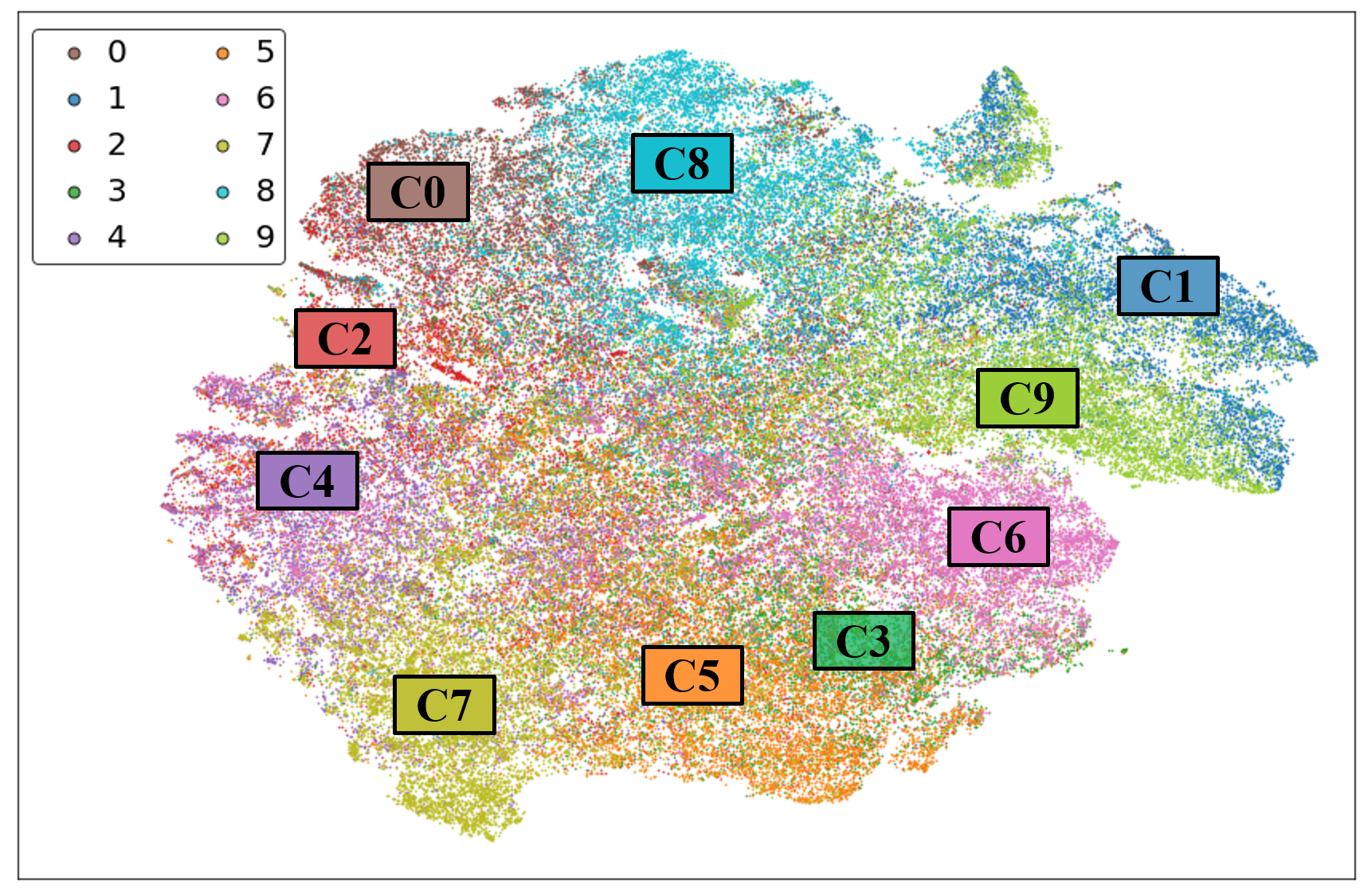
(a) Homogeneous Locals (colored by classes)

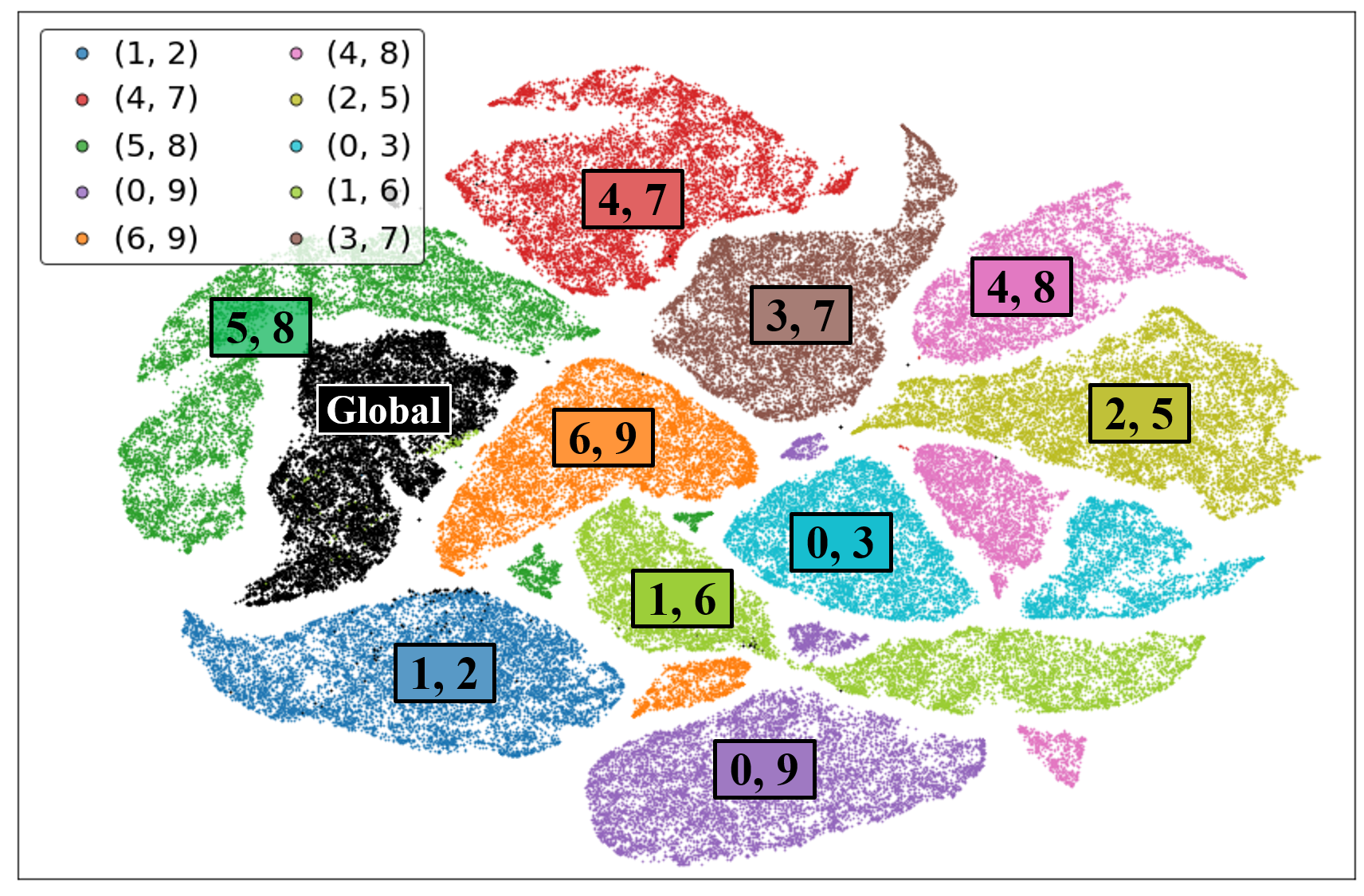
(b) Heterogeneous Locals (colored by locals)

Figure 19: T-SNE visualization of features on CIFAR-10 test samples after local training on (a) homogeneous local distributions and (b) heterogeneous local distributions. The T-SNE is conducted together for the test sample features of global and 10 local models.

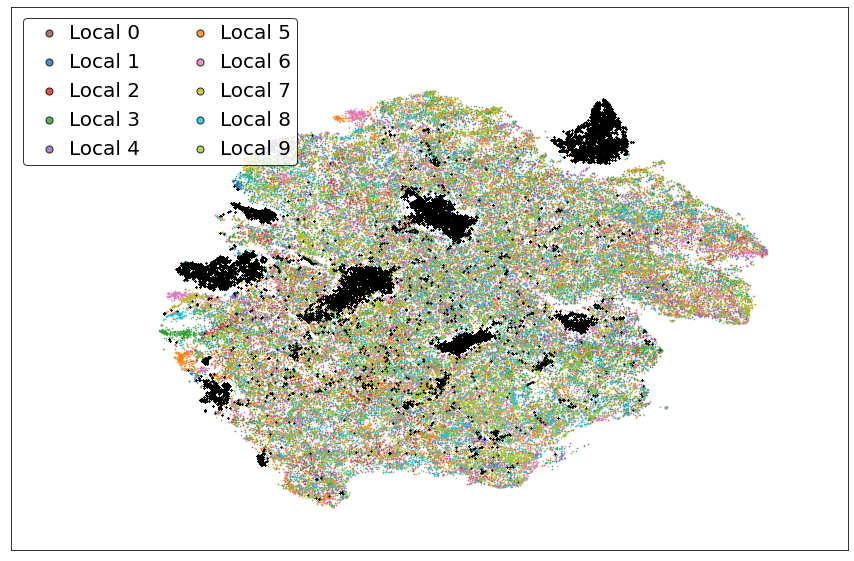
(a) Homogeneous Locals (colored by classes)

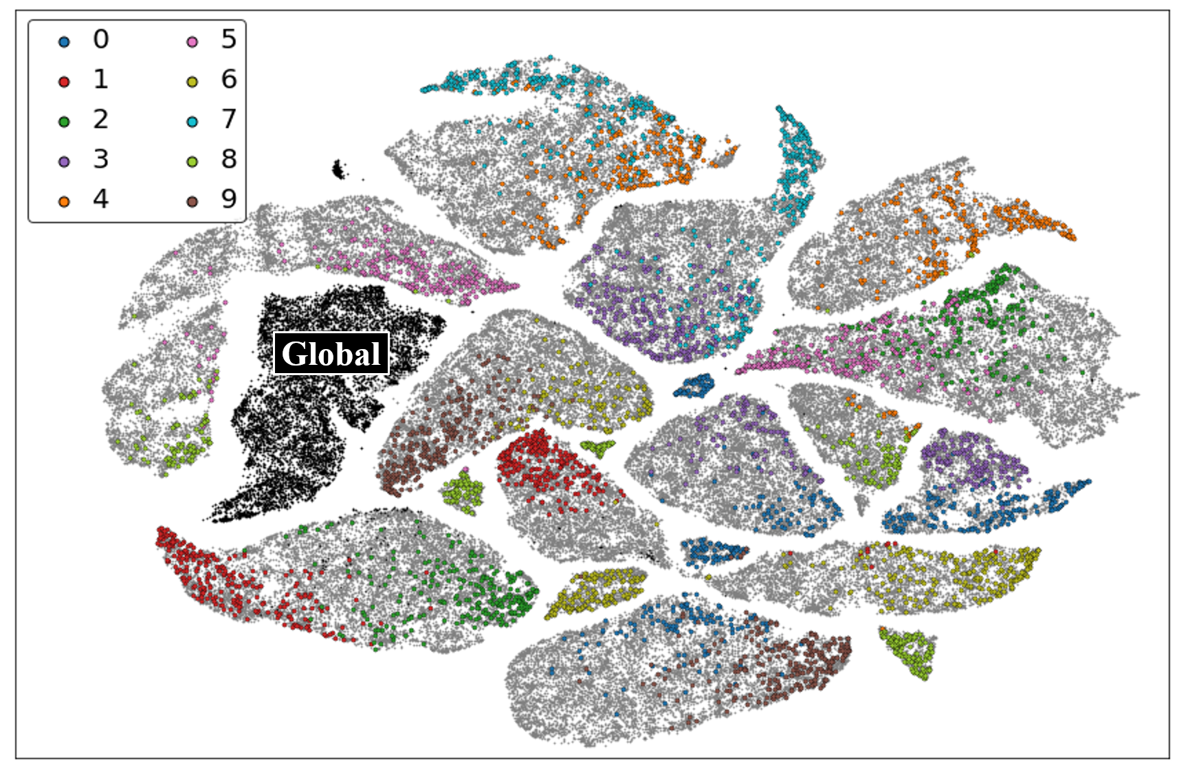
(b) Heterogeneous Locals (colored by locals)

Figure 20: T-SNE visualization of feature region shifting on CIFAR-10 test samples after local training on (a) Homogeneous local distributions and (b) heterogeneous local distributions. The T-SNE is conducted together for the test sample features of global and 10 local models.

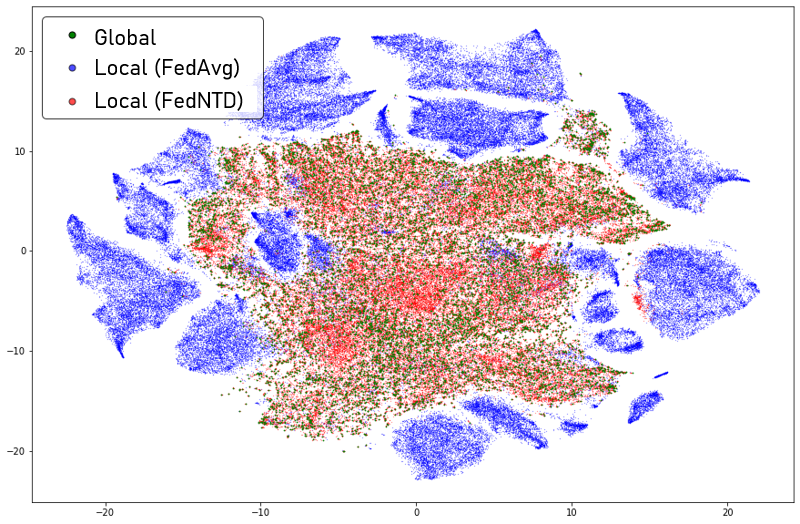
(a) colored by different algorithms

(b) colored by classes

Figure 21: T-SNE on CIFAR-10 testset samples fter local training on heterogeneous local distributions by FedAvg and FedNTD. The T-SNE is conducted together for the test sample features of global and 20 local models (10 for FedAvg and 10 for FedNTD).

Appendix P Proof of Proposition 1

Proof.

Since the class-wise gradient $g_{i}$ are mutually orthogonal and have uniform weight, from the unitarily invariance of the 2-norm we have:

$$\Lambda(\beta) =\frac{\frac{1}{K}\sum_{k=1}^{K}\|p^{k}+\beta\tilde{p}^{k}\|^{2}}{\|\sum_{k=1}^{K}p^{k}+\beta\tilde{p}^{k}\|^{2}}\stackrel{{\scriptstyle(\spadesuit)}}{{=}}\frac{1}{K}\frac{\sum_{k=1}^{K}\sum_{c=1}^{\mathcal{C}}(p^{k}(c)+\beta\tilde{p}^{k}(c))^{2}}{\sum_{c=1}^{\mathcal{C}}(\sum_{k=1}^{K}p^{k}(c)+\beta\tilde{p}^{k}(c))^{2}}$$ (20)

$$\stackrel{{\scriptstyle(\clubsuit)}}{{=}}\frac{1}{(1+\beta)^{2}}\frac{\mathcal{C}}{K^{3}}\sum_{k=1}^{K}\sum_{c=1}^{\mathcal{C}}(p^{k}(c)+\beta\tilde{p}^{k}(c))^{2}$$ (21)

$$=\frac{1}{(1+\beta)^{2}}\frac{\mathcal{C}}{K^{3}}\sum_{k=1}^{K}\mathcal{C}\,\mathbb{E}_{c\in[\mathcal{C}]}[(p^{k}+\beta\tilde{p}^{k})^{2}]=\frac{1}{(1+\beta)^{2}}\frac{\mathcal{C}^{2}}{K^{3}}\sum_{k=1}^{K}\mathbb{E}_{c\in[\mathcal{C}]}[(p^{k}+\beta\tilde{p}^{k})^{2}]$$ (22)

$$=\frac{1}{(1+\beta)^{2}}\frac{\mathcal{C}^{2}}{K^{3}}\sum_{k=1}^{K}\left(\text{Var}_{c\in[\mathcal{C}]}[p^{k}+\beta\tilde{p}^{k}]+(1+\beta)^{2}\right)$$ (23)

$$=\frac{1}{(1+\beta)^{2}}\frac{\mathcal{C}^{2}}{K^{3}}\sum_{k=1}^{K}\left(\text{Var}_{c\in[\mathcal{C}]}\left[p^{k}+\beta\frac{1-p^{k}}{\mathcal{C}-1}\right]\right)+\frac{\mathcal{C}^{2}}{K^{2}}$$ (24)

$$=\frac{1}{(1+\beta)^{2}}\frac{\mathcal{C}^{2}}{K^{3}}\sum_{k=1}^{K}\left(\big{(}1-\frac{\beta}{\mathcal{C}-1}\big{)}^{2}\text{Var}_{c\in[\mathcal{C}]}[p^{k}]\right)+\frac{\mathcal{C}^{2}}{K^{2}}\,.$$ (25)

Where the $(\spadesuit)$ follows from $p^{k}=\sum_{c=1}^{\mathcal{C}}p^{k}(c)\mathbf{e}_{k}(\in\Delta_{\mathcal{C}})$, and $(\clubsuit)$ holds because we are assuming uniform global data distribution. That is, we have the following equation from the symmetry over classes.

$$\sum_{k=1}^{K}p^{k}(c)=\sum_{k=1}^{K}\tilde{p}^{k}(c)=\frac{K}{\mathcal{C}}\,.$$ (26)

By differentiating the equation (25), we have:

$$\frac{\partial\Lambda(\beta)}{\partial\beta} =\left(\frac{\mathcal{C}^{2}}{K^{3}(\mathcal{C}-1)^{2}}\sum_{k=1}^{K}\text{Var}_{c\in[\mathcal{C}]}[p^{k}]\right)\frac{\partial}{\partial\beta}\frac{(\mathcal{C}-(1+\beta))^{2}}{(1+\beta)^{2}}$$ (27)

$$=\left(\frac{\mathcal{C}^{2}}{K^{3}(\mathcal{C}-1)^{2}}\sum_{k=1}^{K}\text{Var}_{c\in[\mathcal{C}]}[p^{k}]\right)\left(-2\frac{\mathcal{C}^{2}}{(1+\beta)^{3}}+2\frac{\mathcal{C}}{(1+\beta)^{2}}\right)$$ (28)

$$=-\left(\frac{2\mathcal{C}^{3}}{K^{3}(\mathcal{C}-1)^{2}}\sum_{k=1}^{K}\text{Var}_{c\in[\mathcal{C}]}[p^{k}]\right)\left(\frac{\mathcal{C}}{(1+\beta)^{3}}-\frac{1}{(1+\beta)^{2}}\right)\,.$$ (29)

∎

By defining $M_{K,\mathcal{C},p}>0$ in the first bracket, we have:

$$\frac{\partial\Lambda}{\partial\beta}=-M_{K,\mathcal{C},p}\left(\frac{\mathcal{C}}{(1+\beta)^{3}}-\frac{1}{(1+\beta)^{2}}\right)\,,$$ (30)

for all $\beta\geq 0$. If $\beta\leq\mathcal{C}/2-1$, we have $\mathcal{C}/(1+\beta)\geq 2$, and get following desired inequality:

$$\frac{\partial\Lambda}{\partial\beta}\leq-M_{K,\mathcal{C},p}\frac{1}{(1+\beta)^{2}}\,.$$ (31)

Appendix Q Proof of Proposition 2

Proof.

First, we show the first equation. The summation for the true class is:

$$\mathcal{L}_{\textup{KL}}^{\textup{true}}=-\frac{1}{N}\sum_{i=1}^{N}q_{\tau}^{g,i}(y_{i})\log\left[\frac{q_{\tau}^{l,i}(y_{i})}{q_{\tau}^{g,i}(y_{i})}\right]$$ (32)

Note that $\sum_{i=1}^{N}=\sum_{c=1}^{\mathcal{C}}\sum_{i\in\mathcal{S}_{c}}$ and $i\in\mathcal{S}_{c}\Rightarrow y_{i}=c$. By using these, we get:

$$\mathcal{L}_{\textup{KL}}^{\textup{true}} =-\frac{1}{N}\sum_{i=1}^{N}q_{\tau}^{g,i}(y_{i})\log\left[\frac{q_{\tau}^{l,i}(y_{i})}{q_{\tau}^{g,i}(y_{i})}\right]=-\frac{1}{N}\sum_{c=1}^{\mathcal{C}}\sum_{i\in\mathcal{S}_{c}}q_{\tau}^{g,i}(c)\log\left[\frac{q_{\tau}^{l,i}(c)}{q_{\tau}^{g,i}(c)}\right]$$ (33)

$$=-\sum_{c=1}^{\mathcal{C}}\>\boldsymbol{p_{c}}\cdot\left(\sum_{i\in\mathcal{S}_{c}}\frac{1}{|\mathcal{S}_{c}|}\>q_{\tau}^{g,i}(c)\log\left[\frac{q_{\tau}^{l,i}(c)}{q_{\tau}^{g,i}(c)}\right]\right)$$ (34)

$$=-\sum_{c=1}^{\mathcal{C}}\>\boldsymbol{p_{c}}\cdot\mathbb{E}_{i\in\mathcal{S}_{c}}\left[q_{\tau}^{g,i}(c)\log\left[\frac{q_{\tau}^{l,i}(c)}{q_{\tau}^{g,i}(c)}\right]\right].$$ (35)

Next, we derive the not-true part of the Kullback-Leibler divergence:

$$-N{\mathcal{L}}_{\text{KL}}^{\text{not-true}}=\sum_{i=1}^{N}\sum_{c^{\prime}\neq y_{i}}^{\mathcal{C}}q_{\tau}^{g,i}(c^{\prime})\log\left[\frac{q_{\tau}^{l,i}(c^{\prime})}{q_{\tau}^{g,i}(c^{\prime})}\right]\,.$$ (36)

By using the double summation technique ($\bigstar$), we have:

$$-N{\mathcal{L}}_{\text{KL}}^{\text{not-true}} =\sum_{c=1}^{\mathcal{C}}\sum_{i\in\mathcal{S}_{c}}\sum_{c^{\prime}\neq c}^{\mathcal{C}}q_{\tau}^{g,i}(c^{\prime})\log\left[\frac{q_{\tau}^{l,i}(c^{\prime})}{q_{\tau}^{g,i}(c^{\prime})}\right]=\sum_{c=1}^{\mathcal{C}}\sum_{c^{\prime}\neq c}^{\mathcal{C}}\sum_{i\in\mathcal{S}_{c}}q_{\tau}^{g,i}(c^{\prime})\log\left[\frac{q_{\tau}^{l,i}(c^{\prime})}{q_{\tau}^{g,i}(c^{\prime})}\right]$$ (37)

$$\stackrel{{\scriptstyle(\bigstar)}}{{=}}\sum_{c^{\prime}=1}^{\mathcal{C}}\sum_{c\neq c^{\prime}}^{\mathcal{C}}\sum_{i\in\mathcal{S}_{c}}q_{\tau}^{g,i}(c^{\prime})\log\left[\frac{q_{\tau}^{l,i}(c^{\prime})}{q_{\tau}^{g,i}(c^{\prime})}\right]=\sum_{c=1}^{\mathcal{C}}\sum_{c^{\prime}\neq c}^{\mathcal{C}}\sum_{i\in\mathcal{S}_{c^{\prime}}}q_{\tau}^{g,i}(c)\log\left[\frac{q_{\tau}^{l,i}(c)}{q_{\tau}^{g,i}(c)}\right]$$ (38)

$$=(\mathcal{C}-1)\sum_{c=1}^{\mathcal{C}}\frac{\sum_{c^{\prime}\neq c}|\mathcal{S}_{c}^{\prime}|}{\mathcal{C}-1}\left(\sum_{c^{\prime}\neq c}\frac{1}{\sum_{c^{\prime}\neq c}|\mathcal{S}_{c^{\prime}}|}{\sum_{i\in\mathcal{S}_{c}^{\prime}}q_{\tau}^{g,i}(c)\log\left[\frac{q_{\tau}^{l,i}(c)}{q_{\tau}^{g,i}(c)}\right]}\right)$$ (39)

$$=(\mathcal{C}-1)\sum_{c=1}^{\mathcal{C}}N\boldsymbol{\tilde{p}_{c}}\>\cdot\mathbb{E}_{i\notin\mathcal{S}_{c}}\left[q_{\tau}^{g,i}(c)\log\left[\frac{q_{\tau}^{l,i}(c)}{q_{\tau}^{g,i}(c)}\right]\right]\,.$$ (40)

∎

Therefore, we get our desired result:

$$\frac{{\mathcal{L}}_{\text{KL}}^{\text{not-true}}}{\mathcal{C}-1}=\sum_{c=1}^{\mathcal{C}}\boldsymbol{\tilde{p}_{c}}\mathbb{E}_{i\notin\mathcal{S}_{c}}\left[q_{\tau}^{g,i}(c)\log\left[\frac{q_{\tau}^{l,i}(c)}{q_{\tau}^{g,i}(c)}\right]\right]\,.$$ (41)

Appendix R Derivation of Equation 15

Proof.

The main part of the proof is well-known inequality for smooth functions, which is derived from the Taylor approximation. Since $\mathcal{L}_{i}\mathrel{\mathop{\mathchar 58\relax}}\mathcal{W}\subset\mathbb{R}^{n}\rightarrow\mathbb{R}$ is smooth function, we have

$$\mathcal{L}_{i}(w) =\mathcal{L}_{i}(w_{i})+\nabla\mathcal{L}_{i}(w_{i})\cdot(w-w_{i})+\int_{0}^{1}(1-t)(w-w_{i})^{\top}\cdot\nabla^{2}\mathcal{L}_{i}(w_{i}+t(w-w_{i}))\cdot(w-w_{i})dt$$ (42)

$$=\mathcal{L}_{i}(w_{i})+\int_{0}^{1}(1-t)(w-w_{i})^{\top}\cdot\nabla^{2}\mathcal{L}_{i}(w_{i}+t(w-w_{i}))\cdot(w-w_{i})dt$$ (43)

$$\leq\mathcal{L}_{i}(w_{i})+\lambda\int_{0}^{1}(1-t)(w-w_{i})^{\top}\cdot(w-w_{i})dt \nabla^{2}\mathcal{L}_{i}(w)\preceq\lambda$$ ()

$$=\mathcal{L}_{i}(w_{i})+\frac{\lambda}{2}\lVert w-w_{i}\rVert^{2}\,.$$ (44)

∎

Appendix S Proof of Proposition 3

Proof.

To show this corollary, enough to show that the below minimax problem is attained on the uniform distribution.

$$\inf_{p\in\Delta_{\mathcal{C}}}\sup_{\mathbb{P}\in\Pi}\mathbb{E}_{p^{\prime}\sim\mathbb{P}}[\lVert p^{\prime}-p\rVert].$$ (45)

Let us define $p\mapsto\sup_{\mathbb{P}\in\Pi}\mathbb{E}_{p^{\prime}\sim\mathbb{P}}[\lVert p^{\prime}-p\rVert]$ as $F(p)$. First, we check the continuity of $F$. That is:

$$|F(p_{2})-F(p_{1})|\leq \left|\sup_{\mathbb{P}\in\Pi}\mathbb{E}_{p^{\prime}\sim\mathbb{P}}[\lVert p^{\prime}-p_{2}\rVert]-\sup_{\mathbb{P}\in\Pi}\mathbb{E}_{p^{\prime}\sim\mathbb{P}}[\lVert p^{\prime}-p_{1}\rVert]\right|$$ (46)

$$\leq \sup_{\mathbb{P}\in\Pi}\bigg{|}\mathbb{E}_{p^{\prime}\sim\mathbb{P}}[\lVert p^{\prime}-p_{2}\rVert-\lVert p^{\prime}-p_{1}\rVert]\bigg{|}\leq\sup_{\mathbb{P}\in\Pi}\mathbb{E}_{p^{\prime}\sim\mathbb{P}}[|\lVert p^{\prime}-p_{2}\rVert-\lVert p^{\prime}-p_{1}\rVert|]$$ (47)

$$\leq \sup_{\mathbb{P}\in\Pi}\mathbb{E}_{p^{\prime}\sim\mathbb{P}}[\lVert p_{1}-p_{2}\rVert]\leq\lVert p_{1}-p_{2}\rVert\,.$$ (48)

Therefore, since the function $F$ is 1-Lipschitz, it is clearly continuous. Now, since $\Delta_{\mathcal{C}}$ is compact, we have a minimizer $p_{0}\in\Delta_{\mathcal{C}}$ of above minimax value. Since norm and expectation is convex function, $F$ is convex. Therefore, for arbitrary minimizer $p_{0}$ and cycle $\sigma=(1\>2\>\cdots\>C)\in\mathcal{S}_{\mathcal{C}}$, we have:

$$F(\text{unif. dist})=F\left(\frac{1}{\mathcal{C}}\sum_{i}\sigma^{i}(p_{0})\right)\leq\frac{1}{\mathcal{C}}\sum_{i}F(\sigma^{i}(p_{0}))\,.$$ (49)

Now, we argue that $F(\sigma^{i}(p_{0}))=F(p_{0})$. From the definition of $F$,

$$F(\sigma^{i}(p_{0})) =\sup_{\mathbb{P}\in\Pi}\mathbb{E}_{p^{\prime}\sim\mathbb{P}}[\lVert p^{\prime}-\sigma^{i}(p_{0})\rVert]=\sup_{\mathbb{P}\in\Pi}\mathbb{E}_{p^{\prime}\sim\mathbb{P}}[\lVert\sigma^{i}(\sigma^{-i}(p^{\prime}))-\sigma^{i}(p_{0})\rVert]$$ (50)

$$=\sup_{\mathbb{P}\in\Pi}\mathbb{E}_{p^{\prime}\sim\mathbb{P}}[\lVert\sigma^{i}(\sigma^{-i}(p^{\prime}))-\sigma^{i}(p_{0})\rVert]$$ (51)

$$=\sup_{\mathbb{P}\in\Pi}\int_{\Delta_{\mathcal{C}}}\lVert\sigma^{i}(\sigma^{-i}(p^{\prime}))-p_{0}\rVert\,d\mathbb{P}(p^{\prime})$$ (52)

$$=\sup_{\mathbb{P}\in\Pi}\int_{\Delta_{\mathcal{C}}}\lVert\sigma^{-i}(p^{\prime})-p_{0}\rVert\,d\mathbb{P}(\sigma^{i}(\sigma^{-i}(p^{\prime})))$$ (53)

$$=\sup_{\mathbb{P}\in\Pi}\int_{\Delta_{\mathcal{C}}}\lVert p^{\prime\prime}-p_{0}\rVert\,d\mathbb{P}(\sigma^{i}(p^{\prime\prime}))$$ (54)

$$=\sup_{\mathbb{P}\in\Pi}\int_{\Delta_{\mathcal{C}}}\lVert p^{\prime\prime}-p_{0}\rVert\,d\mathbb{P}(p^{\prime\prime})=F(p_{0})\,. \Pi \mathcal{S}_{\mathcal{C}} \sigma^{i}\in\mathcal{S}_{\mathcal{C}}$$ ( is -invariant ())

From the equation equation (49), we have:

$$F(\text{unif. dist})\leq\frac{1}{\mathcal{C}}\sum_{i}F(\sigma^{i}(p_{0}))=\frac{1}{\mathcal{C}}\sum_{i}F(p_{0})=F(p_{0})\,.$$ (56)

Since $p_{0}$ is minimizer, we can argue that the uniform distribution also attains the minimum. ∎

References

- [1] Durmus Alp Emre Acar, Yue Zhao, Ramon Matas Navarro, Matthew Mattina, Paul N Whatmough, and Venkatesh Saligrama. Federated learning based on dynamic regularization. arXiv preprint arXiv:2111.04263, 2021.
- [2] Mohammed Aledhari, Rehma Razzak, Reza M Parizi, and Fahad Saeed. Federated learning: A survey on enabling technologies, protocols, and applications. IEEE Access, 8:140699–140725, 2020.
- [3] Rahaf Aljundi, Francesca Babiloni, Mohamed Elhoseiny, Marcus Rohrbach, and Tinne Tuytelaars. Memory aware synapses: Learning what (not) to forget. In Proceedings of the European Conference on Computer Vision (ECCV), pages 139–154, 2018.
- [4] Sungmin Cha, Hsiang Hsu, Taebaek Hwang, Flavio P Calmon, and Taesup Moon. Cpr: Classifier-projection regularization for continual learning. arXiv preprint arXiv:2006.07326, 2020.
- [5] Arslan Chaudhry, Puneet K Dokania, Thalaiyasingam Ajanthan, and Philip HS Torr. Riemannian walk for incremental learning: Understanding forgetting and intransigence. In Proceedings of the European Conference on Computer Vision (ECCV), pages 532–547, 2018.
- [6] Arslan Chaudhry, Albert Gordo, Puneet Kumar Dokania, Philip Torr, and David Lopez-Paz. Using hindsight to anchor past knowledge in continual learning. arXiv preprint arXiv:2002.08165, 2(7), 2020.
- [7] Arslan Chaudhry, Naeemullah Khan, Puneet K Dokania, and Philip HS Torr. Continual learning in low-rank orthogonal subspaces. arXiv preprint arXiv:2010.11635, 2020.
- [8] Arslan Chaudhry, Marc’Aurelio Ranzato, Marcus Rohrbach, and Mohamed Elhoseiny. Efficient lifelong learning with a-gem. arXiv preprint arXiv:1812.00420, 2018.
- [9] Hong-You Chen and Wei-Lun Chao. Fedbe: Making bayesian model ensemble applicable to federated learning. arXiv preprint arXiv:2009.01974, 2020.
- [10] Luke N Darlow, Elliot J Crowley, Antreas Antoniou, and Amos J Storkey. Cinic-10 is not imagenet or cifar-10. arXiv preprint arXiv:1810.03505, 2018.
- [11] Li Deng. The mnist database of handwritten digit images for machine learning research. IEEE Signal Processing Magazine, 29(6):141–142, 2012.
- [12] Terrance DeVries and Graham W Taylor. Improved regularization of convolutional neural networks with cutout. arXiv preprint arXiv:1708.04552, 2017.
- [13] Jiahua Dong, Lixu Wang, Zhen Fang, Gan Sun, Shichao Xu, Xiao Wang, and Qi Zhu. Federated class-incremental learning. arXiv preprint arXiv:2203.11473, 2022.
- [14] Mehrdad Farajtabar, Navid Azizan, Alex Mott, and Ang Li. Orthogonal gradient descent for continual learning. In International Conference on Artificial Intelligence and Statistics, pages 3762–3773. PMLR, 2020.
- [15] Ian J Goodfellow, Mehdi Mirza, Da Xiao, Aaron Courville, and Yoshua Bengio. An empirical investigation of catastrophic forgetting in gradient-based neural networks. arXiv preprint arXiv:1312.6211, 2013.
- [16] Chaoyang He, Songze Li, Jinhyun So, Xiao Zeng, Mi Zhang, Hongyi Wang, Xiaoyang Wang, Praneeth Vepakomma, Abhishek Singh, Hang Qiu, et al. Fedml: A research library and benchmark for federated machine learning. arXiv preprint arXiv:2007.13518, 2020.
- [17] Geoffrey Hinton, Oriol Vinyals, and Jeff Dean. Distilling the knowledge in a neural network. arXiv preprint arXiv:1503.02531, 2015.
- [18] Tzu-Ming Harry Hsu, Hang Qi, and Matthew Brown. Measuring the effects of non-identical data distribution for federated visual classification. arXiv preprint arXiv:1909.06335, 2019.
- [19] Peter Kairouz, H Brendan McMahan, Brendan Avent, Aurélien Bellet, Mehdi Bennis, Arjun Nitin Bhagoji, Keith Bonawitz, Zachary Charles, Graham Cormode, Rachel Cummings, et al. Advances and open problems in federated learning. arXiv preprint arXiv:1912.04977, 2019.
- [20] Sai Praneeth Karimireddy, Satyen Kale, Mehryar Mohri, Sashank Reddi, Sebastian Stich, and Ananda Theertha Suresh. Scaffold: Stochastic controlled averaging for federated learning. In International Conference on Machine Learning, pages 5132–5143. PMLR, 2020.
- [21] Ahmed Khaled, Konstantin Mishchenko, and Peter Richtárik. Tighter theory for local sgd on identical and heterogeneous data. In International Conference on Artificial Intelligence and Statistics, pages 4519–4529. PMLR, 2020.
- [22] James Kirkpatrick, Razvan Pascanu, Neil Rabinowitz, Joel Veness, Guillaume Desjardins, Andrei A Rusu, Kieran Milan, John Quan, Tiago Ramalho, Agnieszka Grabska-Barwinska, et al. Overcoming catastrophic forgetting in neural networks. Proceedings of the national academy of sciences, 114(13):3521–3526, 2017.
- [23] Jakub Konečnỳ, H Brendan McMahan, Daniel Ramage, and Peter Richtárik. Federated optimization: Distributed machine learning for on-device intelligence. arXiv preprint arXiv:1610.02527, 2016.
- [24] Jakub Konečnỳ, H Brendan McMahan, Felix X Yu, Peter Richtárik, Ananda Theertha Suresh, and Dave Bacon. Federated learning: Strategies for improving communication efficiency. arXiv preprint arXiv:1610.05492, 2016.
- [25] Alex Krizhevsky, Vinod Nair, and Geoffrey Hinton. Cifar-10 and cifar-100 datasets. URl: https://www. cs. toronto. edu/kriz/cifar. html, 6, 2009.
- [26] Daliang Li and Junpu Wang. Fedmd: Heterogenous federated learning via model distillation. arXiv preprint arXiv:1910.03581, 2019.
- [27] Qinbin Li, Yiqun Diao, Quan Chen, and Bingsheng He. Federated learning on non-iid data silos: An experimental study. arXiv preprint arXiv:2102.02079, 2021.
- [28] Qinbin Li, Bingsheng He, and Dawn Song. Model-contrastive federated learning. In Proceedings of the IEEE/CVF Conference on Computer Vision and Pattern Recognition, pages 10713–10722, 2021.
- [29] Tian Li, Anit Kumar Sahu, Ameet Talwalkar, and Virginia Smith. Federated learning: Challenges, methods, and future directions. IEEE Signal Processing Magazine, 37(3):50–60, 2020.
- [30] Tian Li, Anit Kumar Sahu, Manzil Zaheer, Maziar Sanjabi, Ameet Talwalkar, and Virginia Smith. Federated optimization in heterogeneous networks. Proceedings of Machine Learning and Systems, 2:429–450, 2020.
- [31] Xiang Li, Kaixuan Huang, Wenhao Yang, Shusen Wang, and Zhihua Zhang. On the convergence of fedavg on non-iid data. arXiv preprint arXiv:1907.02189, 2019.
- [32] Zhizhong Li and Derek Hoiem. Learning without forgetting. IEEE transactions on pattern analysis and machine intelligence, 40(12):2935–2947, 2017.
- [33] Tao Lin, Lingjing Kong, Sebastian U Stich, and Martin Jaggi. Ensemble distillation for robust model fusion in federated learning. arXiv preprint arXiv:2006.07242, 2020.
- [34] Mi Luo, Fei Chen, Dapeng Hu, Yifan Zhang, Jian Liang, and Jiashi Feng. No fear of heterogeneity: Classifier calibration for federated learning with non-iid data. arXiv preprint arXiv:2106.05001, 2021.
- [35] Marc Masana, Xialei Liu, Bartlomiej Twardowski, Mikel Menta, Andrew D Bagdanov, and Joost van de Weijer. Class-incremental learning: survey and performance evaluation on image classification. arXiv preprint arXiv:2010.15277, 2020.
- [36] Michael McCloskey and Neal J Cohen. Catastrophic interference in connectionist networks: The sequential learning problem. In Psychology of learning and motivation, volume 24, pages 109–165. Elsevier, 1989.
- [37] Brendan McMahan, Eider Moore, Daniel Ramage, Seth Hampson, and Blaise Aguera y Arcas. Communication-efficient learning of deep networks from decentralized data. In Artificial Intelligence and Statistics, pages 1273–1282. PMLR, 2017.
- [38] Matias Mendieta, Taojiannan Yang, Pu Wang, Minwoo Lee, Zhengming Ding, and Chen Chen. Local learning matters: Rethinking data heterogeneity in federated learning. In Proceedings of the IEEE/CVF Conference on Computer Vision and Pattern Recognition, pages 8397–8406, 2022.
- [39] Martial Mermillod, Aurélia Bugaiska, and Patrick Bonin. The stability-plasticity dilemma: Investigating the continuum from catastrophic forgetting to age-limited learning effects. Frontiers in psychology, 4:504, 2013.
- [40] German I Parisi, Ronald Kemker, Jose L Part, Christopher Kanan, and Stefan Wermter. Continual lifelong learning with neural networks: A review. Neural Networks, 113:54–71, 2019.
- [41] Adam Paszke, Sam Gross, Francisco Massa, Adam Lerer, James Bradbury, Gregory Chanan, Trevor Killeen, Zeming Lin, Natalia Gimelshein, Luca Antiga, Alban Desmaison, Andreas Kopf, Edward Yang, Zachary DeVito, Martin Raison, Alykhan Tejani, Sasank Chilamkurthy, Benoit Steiner, Lu Fang, Junjie Bai, and Soumith Chintala. Pytorch: An imperative style, high-performance deep learning library. In H. Wallach, H. Larochelle, A. Beygelzimer, F. d'Alché-Buc, E. Fox, and R. Garnett, editors, Advances in Neural Information Processing Systems 32, pages 8024–8035. Curran Associates, Inc., 2019.
- [42] Mark B Ring. Child: A first step towards continual learning. In Learning to learn, pages 261–292. Springer, 1998.
- [43] Neta Shoham, Tomer Avidor, Aviv Keren, Nadav Israel, Daniel Benditkis, Liron Mor-Yosef, and Itai Zeitak. Overcoming forgetting in federated learning on non-iid data. arXiv preprint arXiv:1910.07796, 2019.
- [44] Sebastian U Stich. Local sgd converges fast and communicates little. arXiv preprint arXiv:1805.09767, 2018.
- [45] Sebastian Thrun. Lifelong learning algorithms. In Learning to learn, pages 181–209. Springer, 1998.
- [46] Hongyi Wang, Mikhail Yurochkin, Yuekai Sun, Dimitris Papailiopoulos, and Yasaman Khazaeni. Federated learning with matched averaging. arXiv preprint arXiv:2002.06440, 2020.
- [47] Jianyu Wang, Qinghua Liu, Hao Liang, Gauri Joshi, and H Vincent Poor. Tackling the objective inconsistency problem in heterogeneous federated optimization. arXiv preprint arXiv:2007.07481, 2020.
- [48] Blake Woodworth, Kumar Kshitij Patel, Sebastian Stich, Zhen Dai, Brian Bullins, Brendan Mcmahan, Ohad Shamir, and Nathan Srebro. Is local sgd better than minibatch sgd? In International Conference on Machine Learning, pages 10334–10343. PMLR, 2020.
- [49] Chencheng Xu, Zhiwei Hong, Minlie Huang, and Tao Jiang. Acceleration of federated learning with alleviated forgetting in local training. arXiv preprint arXiv:2203.02645, 2022.
- [50] Qiang Yang, Yang Liu, Tianjian Chen, and Yongxin Tong. Federated machine learning: Concept and applications. ACM Transactions on Intelligent Systems and Technology (TIST), 10(2):1–19, 2019.
- [51] Jaehong Yoon, Wonyong Jeong, Giwoong Lee, Eunho Yang, and Sung Ju Hwang. Federated continual learning with weighted inter-client transfer. In International Conference on Machine Learning, pages 12073–12086. PMLR, 2021.
- [52] Tehrim Yoon, Sumin Shin, Sung Ju Hwang, and Eunho Yang. Fedmix: Approximation of mixup under mean augmented federated learning. In International Conference on Learning Representations, 2021.
- [53] Fuxun Yu, Weishan Zhang, Zhuwei Qin, Zirui Xu, Di Wang, Chenchen Liu, Zhi Tian, and Xiang Chen. Fed2: Feature-aligned federated learning. In Proceedings of the 27th ACM SIGKDD Conference on Knowledge Discovery & Data Mining, pages 2066–2074, 2021.
- [54] Mikhail Yurochkin, Mayank Agarwal, Soumya Ghosh, Kristjan Greenewald, Nghia Hoang, and Yasaman Khazaeni. Bayesian nonparametric federated learning of neural networks. In International Conference on Machine Learning, pages 7252–7261. PMLR, 2019.
- [55] Lin Zhang, Li Shen, Liang Ding, Dacheng Tao, and Ling-Yu Duan. Fine-tuning global model via data-free knowledge distillation for non-iid federated learning. arXiv preprint arXiv:2203.09249, 2022.
- [56] Yue Zhao, Meng Li, Liangzhen Lai, Naveen Suda, Damon Civin, and Vikas Chandra. Federated learning with non-iid data. arXiv preprint arXiv:1806.00582, 2018.
- [57] Yanlin Zhou, George Pu, Xiyao Ma, Xiaolin Li, and Dapeng Wu. Distilled one-shot federated learning. arXiv preprint arXiv:2009.07999, 2020.
- [58] Zhuangdi Zhu, Junyuan Hong, and Jiayu Zhou. Data-free knowledge distillation for heterogeneous federated learning. arXiv preprint arXiv:2105.10056, 2021.