Late time acceleration due to generic modification of gravity and Hubble tension

Abstract

We consider a scenario of modified gravity, which is generic to late-time acceleration, namely, acceleration in the Jordan frame and no acceleration in the Einstein frame. The possibility is realized by assuming an interaction between dark matter and the baryonic component in the Einstein frame which is removed by going to the Jordan frame using a disformal transformation giving rise to an exotic effective fluid responsible for causing phantom crossing at late times. In this scenario, past evolution is not distinguished from $\Lambda$CDM but late time dynamics is generically different due to the presence of phantom crossing that causes a monotonous increase in the expansion rate giving rise to distinctive late-time cosmic feature. The latter can play a crucial role in addressing the tension between the observed value of Hubble parameter by CMB (Cosmic Microwave Background) measurements and the local observations. We demonstrate that the Hubble tension significantly reduces in the scenario under consideration for the chosen scale factor parametrizations. The estimated age of the universe in the model is well within the observational bounds in the low and high red-shift regimes.

1 Introduction

Consistency of standard model of Universe necessarily asks that the hot big bang model be complemented by two phases of accelerated expansion, namely, inflation and late time acceleration [1]. Observation reveals that the age of certain well known objects in the Universe exceeds the age of Universe estimated in the model assuming presence of standard matter in the Universe [2, 6, 3, 4, 5]. Since most of the contribution to the age of Universe comes from late time evolution, thereby, invoking the late time cosmic acceleration slows down the rate of Hubble expansion such that it takes more time to reach a given observed value of the Hubble parameter, in particular, $H_{0}$[7]. And the latter provides with a known resolution of the puzzle. A possibility to ease such a $H_{0}$ tension in case of scalar tensor theories was first proposed in [8, 9]. Later, for non-minimally coupled scalar-tensor theories in Horndeski gravity, the tension is studied in light of the CMB and BAO datasets [10]. It is interesting to note that the late time cosmic acceleration as consistency requirement of hot big bang is supported by direct as well as by the indirect observations [11]-[27], though such a confirmation is yet to be awaited for inflation.

Broadly, there are two ways to achieve late time cosmic acceleration, namely, by adding a source term with large negative pressure (dubbed dark energy) to the energy momentum tensor in the Einstein equations [28, 30, 31, 32, 33, 34, 35, 36, 37, 38, 39, 40, 41, 42, 43, 44] or by modifying geometry of space time $\hat{\rm a}$ la modified gravity. As for dark energy, a plethora of viable candidates, including quintessence, phantom fields, rolling tachyons and others have been investigated in the literature, see Ref.[28] for details. The simplest model of dark energy based upon cosmological constant dubbed $\Lambda$CDM (where $\Lambda$ is the cosmological constant and CDM is the cold dark matter) is under scrutiny at present and there are strong reasons to look beyond[29]. The modified theories of gravity, can generally be though as Einstein theory plus extra degrees of freedom; $f(R)$ gravity, massive gravity and Horndeski provide examples of alternative theories of large scale modification of gravity extensively discussed in the literature[45]. Thus, according to the standard paradigm, late time acceleration is either sourced by the presence of an exotic matter or large scale modification of gravity.

A third possibility that does not invoke extra degrees of freedom or exotic matter, was proposed in[46], see also Ref.[47] on the related theme. In this framework, interaction between Dark Matter(DM) and Baryonic Matter (BM) is assumed in the Einstein frame, thereby, no acceleration in this frame as the total matter still behaves as non-negative pressure fluid. However, an interesting situation arises in the Jordan frame connected to Einstein frame by a disformal transformation. In the Jordan frame, interaction between DM and BM is removed allowing them to adhere to conservation separately. However, an effective term gets generated in the Jordan frame which mimics an exotic fluid providing a possibility to account for late time acceleration. In this picture, one naturally realizes a phantom crossing at late times. Interestingly, conformal coupling is disfavoured by the stability considerations whereas maximally disformal coupling can account for cosmic acceleration in Jordan frame but deceleration in Einstein frame[46]. As a result, in this scenario, the presence of phantom phase in Jordan frame gives rise to sudden future singularity which however could be delayed to distant future by suitably parametrizing the disformal transformation[47]. Let us emphasize that the said framework gives rise to late time acceleration generic to large scale gravity modification: Acceleration in Jordan frame and no acceleration in Einstein frame [48, 49]. It may be noted that $f(R)$ theories fail to satisfy this criteria if local screening is properly implemented [50, 51, 52, 53, 54, 55, 56].

As mentioned before, the $\Lambda$CDM is faced with a puzzle, namely, the disagreement of the value of $H_{0}$ estimated in it using the CMB likelihood with the local measurements. There are several proposals in the literature where the Hubble tension is addressed from different perspectives using early time or late time cosmology [57]-[120]. The latter yields higher values of the Hubble parameter compared to the ones predicted by Planck measurement which assumes $\Lambda$CDM to be the background model. The scenario under consideration conforms to $\Lambda$CDM in the past and causes phantom crossing around the present epoch which gives rise to monotonously increasing Hubble parameter around the present epoch. It is interesting to note that the recently carried out model independent investigations, using combined cosmological data, are in agreement with late time phantom crossing. Let us stress that this behavior is a distinguished feature of the model based upon the aforesaid disformal coupling which might naturally provide us with a possibility to address the Hubble tension.

The plan of the paper is as follows. In section (2), first we describe the basics of cosmological dynamics of disformal coupling between the DM and BM followed by discussion on the parametrizations of the scale factor. In section (3), we describe the technical details of the analyses done using the Monte Carlo Markov Chains (MCMC) simulations using observational data. There we have shown the evidence for the proposed model of ours with respect to the standard $\Lambda$CDM cosmology using the Bayesian Information Criterion (BIC) technique. Finally a summary and the conclusions of this work are given in section (4).

2 Disformal coupling between known components of matter

In this section, we briefly describe the framework which includes mechanism of interaction between BM and DM in the Einstein frame which is then transformed to the Jordan frame using a disformal transformation. Let us consider the following action in the Einstein frame[46],

$$\mathcal{S}=\int d^{4}x\left(\frac{1}{16\pi G}\sqrt{-g}\mathcal{R}+\mathcal{L}_{DM}\{g_{\mu\nu}\}+\mathcal{L}_{BM}\{\widetilde{g}_{\mu\nu}\}\right),$$ (1)

where $\widetilde{g}_{\mu\nu}$ and $g_{\mu\nu}$ designate the Jordan and Einstein frame metric, respectively. Also, the energy momentum tensors in the Jordan and Einstein frames are defined through variational derivatives of matter actions with respect to $\widetilde{g}_{\mu\nu}$ and ${g}_{\mu\nu}$, respectively. In what follows, quantities with a overhead tilde would be associated with Jordan frame. The construct in Eq. (1) implies coupling between DM and BM in the Einstein frame; obviously, their energy densities do not conserve separately but their sum does and exhibits behavior of standard matter. Consequently, in the framework under consideration, evolution would have decelerating character in the Einstein frame. The Jordan frame metric, $\widetilde{g}_{\mu\nu}$, would be constructed from $g_{\mu\nu}$ and parameters that characterize the dark matter; we shall use disformal transformation between Einstein and Jordan frames.

For simplicity, we assume dark matter to be a perfect fluid which then can be represented by a single scalar field,

$$\mathcal{L}_{DM}=\sqrt{-g}P(X);\leavevmode\nobreak\ \leavevmode\nobreak\ \quad X\equiv-g^{\mu\nu}\partial_{\mu}\Theta\partial_{\nu}\Theta\,,$$ (2)

where $\Theta$ denotes the dark matter field. As stated above, the energy momentum tensor $T_{\mu\nu}$ of DM can be obtained by varying the Einstein frame DM action $\mathcal{S}_{DM}$ with respect to $g_{\mu\nu}$ as

$$T_{\mu\nu}\equiv\frac{2}{\sqrt{-g}}\frac{\delta\mathcal{S}_{DM}}{\delta g^{\mu\nu}}=2P,_{X}\partial_{\mu}\Theta\partial_{\nu}\Theta+Pg_{\mu\nu}\,.$$ (3)

The above expression can be written in the standard perfect fluid form, i.e.,

$$T_{\mu\nu}=(\rho_{DM}+P_{DM})u_{\mu}u_{\nu}+P_{DM}g_{\mu\nu},$$ (4)

if we identify $\rho_{DM}$, $P_{DM}$ and $u_{\mu}$ as follows:

$$\rho_{DM}=2P,_{X}(X)X-P(X)\,,\quad P_{DM}=P(X)\,,\quad u_{\mu}=-\frac{1}{\sqrt{X}}\partial_{\mu}\Theta\,.$$ (5)

The BM energy momentum tensor, on the other hand, is defined as

$$\widetilde{T}_{BM}^{\mu\nu}=\frac{2}{\sqrt{-\widetilde{g}}}\frac{\delta\mathcal{S}_{BM}}{\delta\widetilde{g}_{\mu\nu}}\,.$$ (6)

Note that in the Jordan frame, the matter components are not coupled to each other, though the dynamics might look complicated, the energy momentum tensors of both the components are separately conserved. In particular,

$$\widetilde{\nabla}_{\mu}\widetilde{T}_{BM}^{\mu\nu}=0\text{.}$$ (7)

The coupling between DM and BM is accomplished through Jordan frame metric $\widetilde{g}_{\mu\nu}$(appearing in $\mathcal{L}_{BM}$, Eq. (1)) which can be constructed from the Einstein frame metric and dark matter field. The Jordan and Einstein frame metrics are often thought to be related with the each other through conformal transformation between two frames. However, such a transformation is excluded by the stability considerations. A general relation between $\widetilde{g}_{\mu\nu}$, $g_{\mu\nu}$ and $\Theta$ could be of disformal type,

$$\widetilde{g}_{\mu\nu}=R^{2}(X)g_{\mu\nu}+S(X)\partial_{\mu}\Theta\partial_{\nu}\Theta;\leavevmode\nobreak\ \leavevmode\nobreak\ S(X)\equiv\frac{R^{2}(X)-Q^{2}(X)}{X}\text{,}$$ (8)

with $R$ and $Q$ being the arbitrary functions of X. Varying the action with respect to $g_{\mu\nu}$, we obtain, Einstein equations,

$$G_{\mu\nu}=8\pi GT^{eff}_{\mu\nu}\,$$ (9)

$$T^{eff}_{\mu\nu}=T^{DM}_{\mu\nu}+QR^{3}\widetilde{T}_{BM}^{k\lambda}\left(R^{2}g_{k\mu}g_{\lambda\nu}+(2RR,_{X}g_{k\lambda}+S,_{X}\partial_{k}\Theta\partial_{\lambda}\Theta)\partial_{\mu}\Theta\partial_{\nu}\Theta\right),$$ (10)

where the energy momentum tensor for dark matter, $T^{DM}_{\mu\nu}$ is given in (3). The second term in the expression of effective energy momentum tensor, includes coupling of dark matter and baryonic matter. The effective energy momentum tensor reduces to the sum of energy momentum tensors of the two matter components in absence of coupling, i.e., $Q=R=1$. Let us note that $T^{eff}_{\mu\nu}$ is conserved though the energy momentum tensors of individual matter components do not, thus no exotic behavior is expected in the Einstein frame.

2.1 The FRW Evolution equations

Let us now specialize to spatially homogeneous and isotropic background,

$$ds^{2}=-dt^{2}+a^{2}(t)\left(dx^{2}+dy^{2}+dz^{2}\right)$$ (11)

In this case, the coupling functions Q(X) and R(X) depend upon scale factor such that the Jordan frame metric takes following form ,

$$\widetilde{g}_{\mu\nu}=diag\left(-Q^{2}(a),R^{2}(a)a^{2},R^{2}(a)a^{2},R^{2}(a)a^{2}\right)\text{.}$$ (12)

Einstein equations (10) then give rise to following evolution equations in the FRW Universe,

$$3H^{2}=8\pi G\rho_{Tot}\equiv 8\pi G\left(\rho^{eq}_{DM}\sqrt{\frac{X}{X^{eq}}}\left(\frac{a^{eq}}{a}\right)^{3}-P+QR^{3}\widetilde{\rho}_{b}\right)\text{,}$$ (13)

and

$$2\frac{\ddot{a}}{a}+H^{2}=-8\pi G(P+P_{b})\text{,}$$ (14)

where the superscript ’eq’ represents the quantity at the matter-radiation equality epoch and $P$($P_{b}$) denotes the pressure of DM(BM) in the Einstein frame, such that $P_{b}\equiv QR^{3}\widetilde{P}_{b}$. We assume matter to be pressure-less, namely, $\widetilde{P}_{b}\simeq 0\text{ and }P\ll 2XP,_{X}$. Since baryonic matters adheres to conservation in the Jordan frame, we have,

$$\tilde{\rho}_{b}=\frac{\rho_{b}^{eq}}{R^{3}}\left(\frac{a^{eq}}{a}\right)^{3}\,.$$ (15)

Under the said assumptions on $\tilde{P}_{b}$ and $P$, the RHS of (14) vanishes which implies that background in the Einstein frame is matter dominated, i.e., $a(t)\sim t^{2/3}$ throughout. The total matter density in the Einstein frame then acquires the form,

$$\rho_{Tot}(a)=\left(\rho^{eq}_{DM}\sqrt{\frac{X}{X_{eq}}}+Q(X)\rho^{eq}_{b}\right)\left(\frac{a_{eq}}{a}\right)^{3}\,,$$ (16)

where the quantity within the brackets should be constant for an arbitrary function $Q(X)$ as the background in the Einstein frame is matter dominated as it should be.

Let us note that coupling is conformal if $Q=R$ otherwise it is disformal. It turns out that system is plagued with with instability in case of conformal coupling[46]. In what follows, without the loss of generality, we shall adhere to the maximally disformal case, namely, $Q(a)\equiv 1$ leaving with a single function $R$ to deal with. The function, $R(a)$, should be such that the thermal history, known to great accuracy, be left intact. Thereby, the physical scale factor $\widetilde{a}=R(a)a$ should agree with $a$ throughout the entire history and should grow sufficiently fast only at late stages such that the physical scale factor $\widetilde{a}$ in Jordan frame experiences acceleration. In what follows, we shall use convenient the parametrizations for the scale factor, keeping in mind, the mentioned phenomenological features.

2.2 Scale factor: Polynomial parametrization

In order to proceed further, we need to specify the function $R(a)$ that conforms to the said requirements. To this effect, we shall use the following parametrizations, namely, the polynomial and exponential ones, for a concrete realization,

$$a(\widetilde{a})=\widetilde{a}+\alpha\widetilde{a}^{2}+\beta\widetilde{a}^{3}\leavevmode\nobreak\ \leavevmode\nobreak\ \leavevmode\nobreak\ \text{(Polynomial)},$$ (17)

$$a(\widetilde{a})=\widetilde{a}e^{\alpha\widetilde{a}}\leavevmode\nobreak\ \leavevmode\nobreak\ \leavevmode\nobreak\ \leavevmode\nobreak\ \leavevmode\nobreak\ \leavevmode\nobreak\ \leavevmode\nobreak\ \leavevmode\nobreak\ \leavevmode\nobreak\ \leavevmode\nobreak\ \leavevmode\nobreak\ \leavevmode\nobreak\ \leavevmode\nobreak\ \leavevmode\nobreak\ \leavevmode\nobreak\ \leavevmode\nobreak\ \text{(Exponential)}$$ (18)

where $\alpha$ and $\beta$ are real parameters.

In the analysis to follow, we would require to present the cosmological parameters in terms of redshifts in both frames[47],

$$\widetilde{a}=\frac{\widetilde{a}_{0}}{1+\widetilde{z}}\text{ , \ \ }a=\frac{a_{0}}{1+z}\text{,}$$ (19)

Using (19), the Hubble parameter, in case of model (17) can be cast in terms of redshift $\widetilde{z}$ as ,

$$\widetilde{H}(\widetilde{z})=\widetilde{H}_{0}F_{(pol)}(\alpha,\beta,\tilde{z})\equiv\widetilde{H}_{0}\frac{(1+\alpha+\beta)^{\frac{1}{2}}(1+2\alpha+3\beta)\left(1+\widetilde{z}\right)^{\frac{9}{2}}}{\left[\left(1+\widetilde{z}\right)^{2}+\alpha\left(1+\widetilde{z}\right)+\beta\right]^{\frac{1}{2}}\left[\left(1+\widetilde{z}\right)^{2}+2\alpha\left(1+\widetilde{z}\right)+3\beta\right]}\text{,}$$ (20)

which can be written through effective fractional density parameters (see Appendix). The corresponding effective (total) equation of state parameter is given by,

$$\widetilde{w}_{eff}(\widetilde{z})=-\frac{2\dot{\widetilde{H}}}{\leavevmode\nobreak\ 3\widetilde{H}^{2}}=\frac{\alpha\left(5+6\alpha+5\widetilde{z}\right)(1+\widetilde{z})^{2}+\beta(14+23\alpha+14\widetilde{z})(1+\widetilde{z})+18\beta^{2}}{3\{(1+\widetilde{z})^{2}+\alpha(1+\widetilde{z})+\beta\}\{(1+\widetilde{z})^{2}+2\alpha(1+\widetilde{z})+3\beta\}}\text{.}$$ (21)

The dark energy (DE) equation of state $\widetilde{w}_{de}$ can then be obtained from the following relation:

$$\widetilde{w}_{eff}(\widetilde{z})=\widetilde{w}_{M}\Omega^{(0)}_{Meff}+\widetilde{w}_{de}(\widetilde{z})\,\Omega^{(0)}_{DE}\Rightarrow\widetilde{\omega}_{de}(z)=\widetilde{\omega}_{eff}(\tilde{z})/\Omega^{(0)}_{DE}\,.$$ (22)

where $\Omega^{(0)}_{Meff}$ and $\Omega^{(0)}_{DE}$ are the effective matter and DE density parameters, respectively, whereas, $\widetilde{w}_{M}$($\widetilde{w}_{M}=0$) is the equation of state parameter for matter. It is also important to mention that for $\alpha=-0.1523$ and $\beta=-0.0407$, the equation of state parameter for this parametrization approaches its $\Lambda$CDM limit i.e., $w_{de}\to-1$ at the present epoch.

2.3 Scale factor : Exponential parametrization

The Friedmann equation and the effective equation of state parameter for parametrization (18), can be written as

$$\widetilde{H}(\widetilde{z})=\frac{\widetilde{H}_{0}(1+\alpha)(1+\widetilde{z})^{5/2}}{1+\widetilde{z}+\alpha}\exp{\left(\frac{3\widetilde{z}\alpha}{2(1+\widetilde{z})}\right)}\equiv H_{0}F_{(exp)}(\tilde{z},\alpha)\,,$$ (23)

$$\widetilde{w}_{eff}(\widetilde{z})=\frac{5\alpha(1+\widetilde{z})+3\alpha^{2}}{3(1+\widetilde{z})\left[(1+\widetilde{z})+\alpha\right]}\text{ .}$$ (24)

Let us note that in both cases, the dark energy equation of state parameter might assume super negative values at late times with a generic behavior embodied with phantom crossing. It is worth noting that such a phenomenon can not be realized by quintessence field; one needs at least two scalar fields to mimic the phantom crossing. It is interesting that the presence of disformal coupling between known components of matter inevitably gives rise to the mentioned behavior. It should also be emphasized that the coupling between DM and BM is removed in the Jordan frame but the Einstein-Hilbert action gets modified. However, the modification of gravity under consideration is not accompanied by extra degree(s) of freedom but allows to realize super acceleration at late times. Last but not least, acceleration in this framework is generically caused by modification of gravity $\hat{\rm a}$ la acceleration in Jordan frame and deceleration in Einstein frame.

3 Methodology and Analysis

In this section, we shall perform the parametric estimation for both parametrizations (17) and (18) using the late time observational data. In order to do so, and to predict the physical significance for both the parametrizations, one needs to consider the standard form of the Friedmann equations. Since, the parametrization (17) is already formulated in the standard form (see appendix (5.1)), it is also necessary and desirable to obtain the similar form for the parametrization (18). However, in this case, due to the exponential function, it is not tenable and therefore, we resort to the following anzats for the Friedmann equation,

$$\left(\frac{\widetilde{H}(\widetilde{z})}{\widetilde{H}_{0}}\right)^{2} = (1+\alpha)^{A}(1+\widetilde{z})^{3}+B\,e^{C\,\widetilde{z}},$$ (25)

$$\widetilde{H}(\widetilde{z}) = \widetilde{H}_{0}F_{(exp)}(\tilde{z},\alpha),$$ (26)

where $A$, $B$ and $C$ are constants. Note that here we can identify $(1+\alpha)^{A}$ as the effective matter density ($\Omega^{(0)}_{Meff}=(1+\alpha)^{A}$) and $B$ to be the effective DE density ($B=\Omega^{(0)}_{DE}$) at the present epoch. Also, the condition $\Omega^{(0)}_{Meff}+\Omega^{(0)}_{DE}=1$, implies that $(1+\alpha)^{A}+B=1$. By expressing $B$ in terms of $A$, we are finally left with only $A$ and $C$ to fit $F_{exp}(\tilde{z},\alpha)$ with (25). Let us note that the fitting is such that at the present epoch one gets back $\widetilde{H}(\widetilde{z})=\widetilde{H_{0}}$, as usual. Whereas, at any $\widetilde{z}\neq 0$, one always sees the presence of $\alpha$ in the Friedmann equation. Using numerical techniques (in particular, non linear model fitting in the Mathematica software), we obtain $A=3.4185$ and $C=0.2896$.

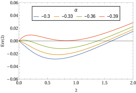
Figure 1: The figure shows the relative error between fitted and the exact Friedmann equation with $z\in[0,2]$ for different values of $\alpha$.

In fig. (1), we plot the relative error between the fitted parametrization (25) with respect to the Eq. (23). In particular, we plot the error function $Err\equiv(E_{fit}-E)/E$ (where $E\equiv\widetilde{H}/\widetilde{H_{0}}$). In this plot we can see that the fitting is reasonably good atleast up to redshift ($\widetilde{z}\leq 2$) for different possible values of $\alpha$.

After formulating the Friedmann equation (23) in the standard form (25), we can extract out the effective DE equation of state $\widetilde{w}_{de}(\widetilde{z})$ from Eq. (22) and can constrain it by using the observational data. Since, we have already expressed the effective equation of state of the system (see Eq. (24)), then it follows that

$$\widetilde{w}_{de}(\widetilde{z})=-\frac{\alpha\,e^{-0.2896\widetilde{z}}\left[\alpha+1.6667(\widetilde{z}+1)\right]}{\left[(\alpha+1)^{3.4185}-1\right](\widetilde{z}+1)(\alpha+\widetilde{z}+1)}\,,$$ (27)

where we have used the fitted value of $B$ and $C$ for $\Omega^{(0)}_{DE}$. Note that for $\alpha=-0.3896$, the exponential parametrization approaches its $\Lambda$CDM model i.e., $\widetilde{w}_{de}(0)=-1$ at the present epoch.

3.1 Data

We have combined three set of data for our analysis. We have taken into account the distance modulus measurement of type Ia supernovae (SNIa), observational Hubble data (OHD) and angular diameter distances measured using water megamasers. The analysis is done in the following way:

3.1.1 Supernova Type Ia - Pantheon Sample

$z$	$E(z)$	Correlation matrix
$0.07$	$0.997\pm 0.023$	$1.00$
$0.20$	$1.111\pm 0.020$	$0.39$	$1.00$
$0.35$	$1.128\pm 0.037$	$0.53$	$-0.14$	$1.00$
$0.55$	$1.364\pm 0.063$	$0.37$	$0.37$	$-0.16$	$1.00$
$0.90$	$1.52\pm 0.12$	$0.01$	$-0.08$	$0.17$	$-0.39$	$1.00$

Table 1: $z$ versus $E(z)$ data together with the correlation matrix between data points obtained from the Supernovae Type-1a Pantheon data [124]

.

In [123], Reiss et al. had presented Hubble rate $E(z_{i})=H(z_{i})/H_{0}$ data points for six different redshifts in the range $z\in[0.07,1.5]$ effectively compressing the information of the - Pantheon compilation [122] and $15$ Sn1a at $z>1$ of the CANDELS and CLASH Multi-Cycle Treasury (MCT) programs obtained by the Hubble Space Telescope (HST), 9 of which are at $1.5<z<2.3$. We have used this data and is enlisted in Table (1). Following the arguments given in [124] we have also omitted the data point at $z=1.5$ from the Table 6 in [123].

Theoretically, the dimensionless Hubble rate $\tilde{h}$ is defined as $\frac{\widetilde{H}(\widetilde{z})}{\widetilde{H_{0}}}$ and hence $\chi^{2}$ for the Supernova data is calculated as

$$\chi^{2}_{\rm{SN}}=\sum_{i,j}\left(E_{i}-\tilde{h}_{i}\right)\cdot c_{ij}^{-1}\cdot\left(E_{i}-\tilde{h}_{i}\right)\,,$$ (28)

where $c_{ij}$ is the correlation matrix given in table (1).

3.1.2 Observational Hubble Data(OHD)

We use the observational measurements of Hubble parameter at different redshifts in the range $0.07<z<1.965$. In particular, we consider a compilation of $31$ $H(z)$ measurements obtained from the cosmic chronometric method [125] and the compiled data set is presented in Table (2).

$z$	$H_{obs}$	$\sigma_{H}$	Reference
0.07	69	19.6	[127]
0.09	69	12	[128]
0.12	68.6	26.2	[127]
0.17	83	8	[128]
0.179	75	4	[125]
0.199	75	5	[125]
0.2	72.9	29.6	[127]
0.27	77	14	[128]
0.28	88.8	36.6	[127]
0.352	83	14	[125]
0.38	81.9	1.9	[126]
0.3802	83	13.5	[129]
0.4	95	17	[128]
0.4004	77	10.2	[129]
0.4247	87.1	11.2	[129]
0.4497	92.8	12.9	[129]
0.47	89	50	[130]

$z$	$H_{obs}$	$\sigma_{H}$	Reference
0.4783	80.9	9	[129]
0.48	97	62	[130]
0.51	90.8	1.9	[126]
0.593	104	13	[125]
0.61	97.8	2.1	[126]
0.68	92	8	[125]
0.781	105	12	[125]
0.875	125	17	[125]
0.88	90	40	[130]
0.9	117	23	[128]
1.037	154	20	[125]
1.3	168	17	[128]
1.363	160	33.6	[131]
1.43	177	18	[128]
1.53	140	14	[128]
1.75	202	40	[128]
1.965	186.5	50.4	[131]

Table 2: Observational hubble data $H_{obs}$ in the units of km s^-1 Mpc^-1 with their corresponding uncertainties $\sigma_{H}$ for various redshifts.

Theoretically we calculate Hubble parameter at different redshifts for our models in different parametrizations as $\widetilde{H}(\widetilde{z})=\widetilde{H_{0}}\times E(\widetilde{z})$, where $\widetilde{H_{0}}$ is the present value of the Hubble parameter. We rescale the present value of the Hubble parameter $\widetilde{H_{0}}$ to $\widetilde{h}$ where $\widetilde{h}=\widetilde{H_{0}}/$(100 km sec^-1 Mpc^-1) and treat $\widetilde{h}$ as a free parameter in our analysis.The $\chi^{2}$ for the Hubble parameter measurements is

$$\chi^{2}_{H}=\sum_{i}\bigg{[}\frac{H_{i}^{th}-H_{i}^{obs}}{\sigma^{H}_{i}}\bigg{]}^{2}$$ (29)

where $H^{\rm{obs}}$ is the observed data from the cosmic chronometer measurements and galaxy distribution measurements given in Table 2, $H^{\rm{th}}$ is the Hubble parameter of our model, $\sigma_{i}^{H}$ is the standard deviation at different redshift in Table 2.

3.1.3 Masers Data :

We have also used the angular diameter distances measured by Megamaser Cosmology Project using water megamasers. The Megamaser data we have used in this analysis is given in Table 5 of [132]. For the sake of completeness we repeat the Table here 3. $\chi^{2}_{\rm{masers}}$ is defined conventionally as

$$\chi^{2}_{\rm{mas}}=\sum_{i}\bigg{[}\frac{D_{Ai}^{th}-D_{Ai}^{obs}(z_{i})}{\sigma^{D}_{i}}\bigg{]}^{2}$$

where $D_{A}^{th}$ is the angular diameter distance for the cosmological model calculated using definition :

$$D_{A}(z)=\frac{1}{1+z}\int_{0}^{z}\frac{dz^{\prime}}{H(z^{\prime})}$$ (30)

Table 3: Megamaser data

Maser	Redshift	Constraint	Ref.
UGC 3789	$z=0.0116$	$\frac{D_{A}(0.0116)}{\rm{Mpc}}=49.6\pm 5.1$	[133]
NGC 6264	$z=0.0340$	$\frac{D_{A}(0.0340)}{\rm{Mpc}}=144\pm 19$	[134]
NGC 5765b	$z=0.0277$	$\frac{D_{A}(0.0277)}{\rm{Mpc}}=126.3\pm 11.6$	[135]

3.2 Analysis

We have performed the statistical analysis with Bayesian inference technique, which is extensively used for parameter estimation in cosmological models. According to this statistics the posterior probability distribution function of the model parameters is proportional to the likelihood function and the prior probability of the model parameters. To estimate the parameters, the likelihoods used are commonly multivariate Gaussian likelihoods given by.

$${\cal L}(\Theta)\propto{\rm exp}\left[-\frac{\chi^{2}(\Theta)}{2}\right]\,,$$ (31)

where $\Theta$ is a set of model parameters. In this analysis we have used uniform prior. So the posterior probability is proportional to ${\rm exp}[-\frac{\chi^{2}(\Theta)}{2}]$. Thus a minimum $\chi^{2}(\Theta)$ will ensure a maximum likelihood or a maximum posterior probability. In our analysis the Gaussian likelihood is given by

$${\cal L}\propto{\rm exp}\left[-\frac{\chi^{2}_{\rm TOT}}{2}\right]\,,$$ (32)

where $\chi^{2}_{\rm TOT}=\chi^{2}_{\rm SN}+\chi^{2}_{\rm H}+\chi^{2}_{\rm masers}$.

parameters	Priors
	Exponential	Polynomial
$\alpha$	[-1 , 0 ]	[-0.5 ,0 ]
$\beta$	-	[ -0.2, 0 ]
$\widetilde{h}$	[0.55 ,0.85 ]	[0.55 , 0.85]

Table 4: Priors for the MCMC parameters

We have constrained different set of parameters for each parametrizations in our analysis. For the Polynomial parametrization the constrained parameters are $\alpha$, $\beta$ and $\widetilde{h}$. Similarly for the exponential parametrization we have constrained $\widetilde{h}$ and $\alpha$. As mentioned earlier in this analysis we have used uniform priors. We have enlisted the priors that we have used for each parametrizations in table 4. We have used Markov Chain Monte Carlo (MCMC) method to make the parameter estimation. For this purpose we have used MCMC sampler, EMCEE,[136, 137] in PYTHON. We have studied these MCMC chains using the program GetDist [138].

3.3 Constraints on Hubble parameter and dark energy equation of state parameter: Phantom crossing and Hubble tension

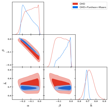
Figure 2: Polynomial: $2\sigma$ contour levels between $\alpha$, $\beta$ and $\widetilde{h}$ for OHD and its combinations with Pantheon+Masers.

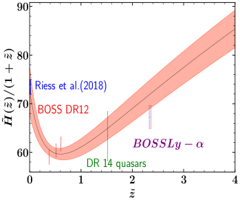
(a)

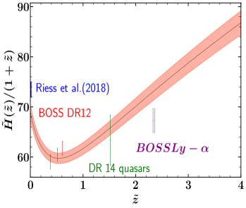
(b)

Figure 3: Polynomial: Figures (3(a)) and (3(b)) depicts the evolution of $\widetilde{H}(\widetilde{z})/(1+\widetilde{z})$ with $\widetilde{z}\in[0,4]$ for the datasets OHD and OHD+Pantheon+Masers, respectively. The dark line represents the best-fit and the shaded region corresponds to the $1\sigma$ limit.

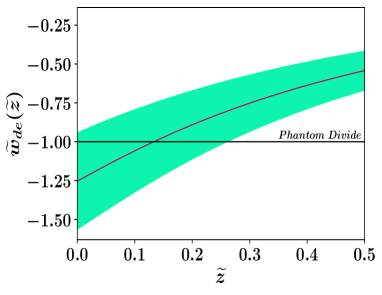
(a)

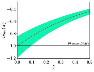
(b)

Figure 4: Polynomial: Figures (4(a)) and (4(b)) depicts the evolution of $\widetilde{w}_{de}(\widetilde{z})$ with $\widetilde{z}\in[0,4]$ for the datasets OHD and OHD+Pantheon+Masers, respectively. The dark line represents the best-fit and the shaded region corresponds to the $1\sigma$ limit.

From the obtained values of parameters $\alpha$, $\beta$ and $\widetilde{h}$, from our MCMC simulation, upto $2\sigma$ (shown in fig.2), we can plot the evolutionary profiles of $\widetilde{H}(\widetilde{z})$ and $\widetilde{w}_{de}(\widetilde{z})$ .

	Parametrizations
Observational	Polynomial	Exponential	$\Lambda$CDM
dataset	Best-fit($\pm 1\sigma$)	Best-fit($\pm 1\sigma$)
	$\widetilde{h}=0.7279_{-0.05}^{+0.05}$	$\widetilde{h}=0.671_{-0.029}^{+0.029}$	$\widetilde{h}=0.6770^{+0.030}_{-0.030}$
OHD	$\alpha=-0.101^{+0.07}_{-0.077}$	$\alpha=-0.299^{+0.043}_{-0.042}$	$\widetilde{\Omega}_{M}=0.3249^{+0.064}_{-0.059}$
	$\beta=-0.078^{+0.051}_{-0.049}$	-
	$\widetilde{h}$ = $0.689_{-0.015}^{+0.015}$	$\widetilde{h}$ = $0.677_{-0.007}^{+0.007}$	$\widetilde{h}=0.6683^{+0.026}_{-0.026}$
OHD+Pantheon +Masers	$\alpha=-0.145^{+0.078}_{-0.051}$	${\alpha}$ = $-0.335_{-0.017}^{+0.016}$	$\widetilde{\Omega}_{M}=0.3440^{+0.061}_{-0.054}$
	$\beta=-0.041^{+0.029}_{-0.047}$	-

Table 5: Best-fits with their $1\sigma$ levels for polynomial and exponential parametrizations, and for the $\Lambda$CDM model from OHD and OHD+Pantheon+Masers datasets.

In fig.2, we have plotted the obtained parametric dependence between $\alpha$, $\beta$ and $\widetilde{h}$ using OHD and its combination with Pantheon and Masers. From this figure, one can note that the combination of all data set significantly reduces the errors bars on $\widetilde{h}$ as compared to only OHD data set. The obtained results are given in table (5) where we show that only OHD data set gives $\widetilde{h}$ significantly larger than the combined data set. In particular, we have not found any significant Hubble tension for OHD, even for the combined data set, the tension reduces to $1.3\sigma$ level. The reduction of this tension can be attributed to the phantom crossing taking place in case of the polynomial parametrization.

The corresponding evolution of $\widetilde{w}_{de}(\widetilde{z})$ and $\widetilde{H}(\widetilde{z})$ upto $1\sigma$ are shown in figures (3) and (4), respectively. In the fig (3), one can see that due to large $1\sigma$ deviations, the only OHD data set does not show a tension with the Riess et. al. [139] and BOSSLy-$\alpha$ [140, 141], whereas the combined data set by giving rise to comparatively small $\widetilde{h}$ shows a significant tension with the Riess et. al. (3). On the other hand, in fig. (4), we show that both of the data sets gives rise to a consequential amount of phantom crossing at present epoch. It is interesting to note that this feature, without adding any extra degrees of freedom, is solely happening due to the coupling between two components of matter (BM and DM).

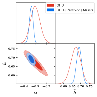
Figure 5: Exponential: $2\sigma$ contour levels between $\alpha$ and $\widetilde{h}$ for OHD and its combinations with Pantheon+Masers.

We also perform the similar analysis for the second parametrization, where in this case we show the parametric dependence between $\alpha$ and $\widetilde{h}$ for two sets of data in fig. (5) and the resulted constraints are shown in the table (5). Here, the value of the Hubble constant is consistent rather with the $DES+BAO+Planck$ combined data in the $1$-$\sigma$ level (see table (2) and Eq. (45) of [142]). Thus, there is no reduction of the tension to significant order. This is expected as in the case of exponential parametrization, there is no phantom crossing (before the present epoch) thus the model mimics the $\Lambda$CDM. The Friedmann equation of the latter can be written as : $\widetilde{H}(\widetilde{z})=100\widetilde{h}\left(\widetilde{\Omega}_{M}(1+\widetilde{z})^{3}+1-\widetilde{\Omega}_{M}\right)$ where $\widetilde{\Omega}_{M}$ is the matter density parameter.

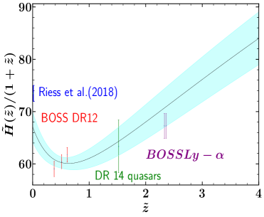
(a)

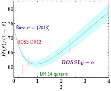
(b)

Figure 6: Exponential: Figures (6(a)) and (6(b)) depicts the evolution of $\widetilde{w}_{de}(\widetilde{z})$ with $\widetilde{z}\in[0,4]$ for the datasets OHD and OHD+Pantheon+Masers, respectively. The dark line represents the best-fit and the shaded region corresponds to the $1\sigma$ limit.

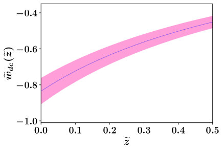
(a)

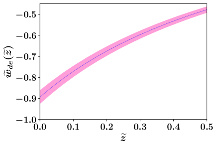
(b)

Figure 7: Exponential: Figures (7(a)) and (7(b)) depicts the evolution of $\widetilde{w}_{de}(\widetilde{z})$ with $\widetilde{z}\in[0,4]$ for the datasets OHD and OHD+Pantheon+Masers, respectively. The dark line represents the best-fit and the shaded region corresponds to the $1\sigma$ limit.

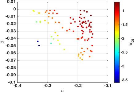
(a)

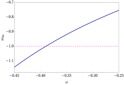
(b)

Figure 8: Exponential: Figures (8(a)) and (8(b)) shows the variation of the two model parameters with equation of state of the dark energy ($w_{DE}$)

Let us note that from the two considered parametrizations, the polynomial case is much better suited to address the Hubble tension. And this can also be understood from the perspective of statistical significance which is discussed in details in the subsection 3.5.

From fig. (6), we see that unlike the polynomial case, the combined data set agrees both with Riess et. al. and BOSSLy-$\alpha$, which is not the case when using only OHD data set. Moreover, from the fig. (7), one can notice that the phantom crossing of $\widetilde{w}_{de}(\widetilde{z})$ does not happen. In fig. (8), we explicitly show the dependence of model parameters on the $\widetilde{w}_{de}$. In fig. (8(a)), we show that in order to give obtain the phantom crossing both $\alpha$ and $\beta$ should be negative, similarly, for the exponential case the dependence of $\widetilde{w}_{de}$ on parameter $\alpha$ is shown in fig. (7).

3.4 Age of objects in the Universe

	Parametrizations
Observational	Polynomial	Exponential
dataset	Best-fit($\pm 1\sigma$)	Best-fit($\pm 1\sigma$)
OHD	$\widetilde{t}(0)$ = $13.657_{-0.421}^{+0.428}$ Gyr	$\widetilde{t}(0)$ = $13.698_{-0.308}^{+0.307}$ Gyr
OHD+Pantheon +Masers	$\widetilde{t}(0)=13.917^{+0.366}_{-0.369}$ Gyr	$\widetilde{t}(0)$ = $13.526_{-0.237}^{+0.237}$ Gyr

Table 6: Age of the Universe with their $1\sigma$ levels for polynomial and exponential parametrizations for OHD and OHD+Pantheon+Masers datasets.

In case of quintessence, the lower bound on its equation of state parameter $\omega_{q}=-1$. When effective equation of state reaches this limit, $w_{q}$ is close to $-1$. The late time acceleration is essential for the consistence of hot big bang with observation on the age of universe. Indeed, as acceleration commences ($\tilde{z}\sim 0.5$), the Hubble expansion rate slows down, thereby, it takes more time to reach a particular value of the Hubble parameter, for instance, $\widetilde{H}_{0}$ and this substantially improves the age of Universe compared to its counter part estimated in absence of late phase of accelerated expansion. In our framework, we have phantom crossing, and compared to the quintessence, in this case, we expect further improvement in age estimate till we cross quintessence lower bound. However, after phantom crossing, the Hubble parameter starts increasing and might match with the one obtained from local observations. But the latter might somewhat suppress the age compared the estimate obtained in the presence of quintessence. Secondly, there are few observations on age of high red-shift objects and since the model under consideration not very different from quintessence or $\Lambda$CDM in the past, it is expected that it would well reconcile with the said data. It is therefore necessary to check, how well, the age of universe in the scenario compares with both the high and low redshift data, Planck and Globular cluster data, respectively.

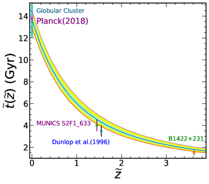
(a)

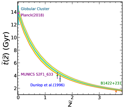
(b)

Figure 9: Polynomial: Figures (9(a)) and (9(b)) depict the evolution of $\widetilde{t}_{de}(\widetilde{z})$ with $\widetilde{z}\in[0,4]$ for the datasets OHD and OHD+Pantheon+Masers, respectively. The dark line represents the best-fit, the green and yellow shaded region corresponds to the $1\sigma$ and $2\sigma$ limits respectively.

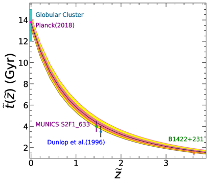
(a)

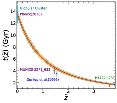
(b)

Figure 10: Exponential: Figures (10(a)) and (10(b)) depicts the evolution of $\widetilde{t}_{de}(\widetilde{z})$ with $\widetilde{z}\in[0,4]$ for the datasets OHD and OHD+Pantheon+Masers, respectively. The dark line represents the best-fit , the orange and yellow shaded region corresponds to the $1\sigma$ and $2\sigma$ limits respectively.

The age of Universe, for both parametrizations, (17) and (18), is given by,

$$\tilde{t}_{(\tilde{z})}=\frac{1}{\widetilde{H}_{0}}\int_{\tilde{z}}^{\infty}{\frac{d\tilde{z}}{F(\tilde{z})}}$$ (33)

where the function $F$ reads as follows,

$$F(\tilde{z})=\begin{cases}&F_{(poly)}(\alpha,\beta,\tilde{z})\leavevmode\nobreak\ \leavevmode\nobreak\ \leavevmode\nobreak\ \text{Polynomial parametrization}\\ &F_{(exp)}(\tilde{z},\alpha)\leavevmode\nobreak\ \leavevmode\nobreak\ \leavevmode\nobreak\ \text{Exponential parametrization}\end{cases}$$ (34)

where $F_{(poly)}$ and $F_{(exp)}$ are given in Eqs.(25) and (20) respectively.

From the obtained constraints, we have found the age of the universe $\widetilde{t}_{de}(\widetilde{z})$ and the corresponding constraints on $\widetilde{t}_{de}(\widetilde{0})$ as shown in table (6) for both parametrizations (17) and (18). Fig. (9) and (10) show the age of the Universe at a given red-shift for the two paramerizations. These figures also include data points of two high redshift galaxies and the quasar $B1422+231$ along with the globular cluster and Planck’18 results [2, 6, 3, 4, 5, 7] for comparison. Our results for both the cases are consistent with the requirement that the Universe be older than any of its constituents at a given red-shift.

3.5 Comparison with $\Lambda$CDM

To compare the two parametrizations, polynomial (17)) and exponential( (18)) with the vanilla $\Lambda$CDM model, one needs to take care of the introduction of the extra degrees of freedom with respect to the standard model. In case of polynomial, we have two extra degrees of freedom and in case of exponential, we have one extra degree of freedom. Thus, a detailed Bayesian Information Criterion (BIC) [143, 144] (following [145]) is calculated to take care of that. BIC analysis penalises a model with extra number of degrees of freedom. Thus, to have strong evidence in support of the model with extra degrees of freedom means much better agreement with observation with respect to the model with less number of degrees of freedom. Under the assumption that the model errors are independent and obey a normal distribution, then the BIC can be rewritten in terms of $\Delta\chi^{2}$ as $BIC\approx\Delta\chi^{2}+df.ln(n)$, where, $df$ is the number of degrees of freedom in the test and $n$ is the number of points in the observed data. The details of our findings are given in the Table (7). One can see from Table (7), the polynomial parametrization has clearly strong evidence with respect to the standard $\Lambda$CDM scenario. Any evidence where $\Delta BIC\geq 10$ reflects very strong evidence for the new model postulated with respect to the standard one. While, the exponential case has positive evidence in case of the combined data, there is no significant evidence of it when the OHD data is only considered. For the polynomial parametrization, we find strong evidence for both OHD as well as combined data.

Observational Dataset	Polynomial ($\Delta$ BIC)	Polynomial Evidence	Exponential ($\Delta$ BIC)	Exponential Evidence
OHD	9.63	Strong	0.62	Not worth
OHD+Pantheon +Masers	8.88	Strong	4.01	Positive

Table 7: The evidence in support of polynomial and exponential parametrizations for OHD and OHD+Pantheon+Masers datasets with respect to the standard $\Lambda$CDM scenario.

4 Conclusion and future perspectives

In this paper, we have investigated the observational viability and generic implications of the dark matter and baryonic matter interaction in the Einstein frame, which is caused by a general disformal transformation between the Jordan and the Einstein frames. In particular, the phenomenon is based upon the assumption that dark matter follows the Einstein frame geodesics, whereas, the baryonic matter obeys Jordan frame trajectories. Consequently, under the standard disformal transformation, a coupling is induced between both the matter components which spoils their individual energy conservation in the Einstein frame.

As the geodesics of both frames are not equivalent (due to the disformal transformation between them), we choose two different parametrizations to relate the scale factors of both the frames in the standard FRW space-time. In particular, we resort to the polynomial and exponential parametrizations and find the constraints on the model parameters in the Jordan frame considering it to be the physical frame (as the underline mechanism assumes the baryonic matter to follow its trajectories in the Jordan frame and hence all the observations are being done in this frame). In case of the polynomial parametrization Eqn. (17), the best-fit values of Hubble parameter for two different data combinations is such that it significantly reduces the so called ‘Hubble tension’. For OHD data, the tension is insignificant in case of polynomial parametrization, as the computed value of $\widetilde{h}=0.7279^{+0.05}_{-0.05}$ $1$-$\sigma$ consistent with Riess et al., whereas for the combined OHD+Pantheon+Masers data, the tension is reduced to $1.3$-$\sigma$ level. We would like to once again emphasise that this is related to the fact that, in this particular parametrization, the dark energy equation of state crosses from quintessence to phantom region. Hence, we see a strong evidence in support of this parametrization while performing the $\Delta$BIC analysis which is quoted in table (7).

As for the exponential parametrization (Eqn. 18), we have not found any significant reduction of Hubble-tension (see, fig. (5)) with both the data combinations and this can be attributed to the fact that, the model exhibits quintessence like behavior with $\widetilde{w}_{de}(\widetilde{z})\geq-1$ around the present epoch. Thus as expected, in the exponential case, we only find some positive evidence in combined data scenario but not significant enough when only OHD is considered (see table (7)). However, the desired behaviour is achieved in case of the polynomial parametrization where phantom-crossing takes place. To this effect, a universal Bayesian evidence calculation could robustly support our claim.

In the framework under consideration, the behavior of the Hubble parameter at late times is generically different from quintessence which is also reflected on the estimate of age of Universe. While for checking the consistency with the globular clusters, Planck 2018 results and the high red-shift data, we find an excellent agreement with observations for both the parametrizations (see figs. (9(a), 9(b)) and (10(a), 10(b))).

It is worth emphasizing that the scenario based upon interaction between DM and BM admits late-time cosmic acceleration without invoking any exotic fluid and it is compatible with observation. One of the most important and generic implications of the interaction at the background level includes the presence of phantom-crossing which is supported by most of the observations at present.

It will be interesting to address the issues like Hubble tension using the different dynamical realisation of the early time acceleration , say, ‘warm’ inflation [146, 147] in this framework. Also in case of non-canonical realisation of inflation [148], one observes non standard sound speed ($c_{s}$) which then can have implications on the measured value of $\widetilde{H}_{0}$ from CMB. The baryon asymmetry of the Universe can be studied also in this framework based on the ideas proposed in [150, 151, 152, 153] the In our opinion, this is an interesting investigation to be carried out within the framework of the model considered here. Last but not least, it would be interesting to consider perturbations and study matter power spectrum in the presence of disformal coupling between DM and BM following Refs. [149, 154]. We would like to address all these issues in our upcoming endeavors.

Acknowledgments: The authors would like to thank Akash Garg, Nur Jaman, Sibesh K. Jas Pacif, Ruchika and Somasri Sen for useful discussions. Work of MRG is supported by Department of Science and Technology(DST), Government of India under the Grant Agreement number IF18-PH-228 (INSPIRE Faculty Award) and by Science and Engineering Research Board(SERB), Department of Science and Technology(DST), Government of India under the Grant Agreement number CRG/2020/004347(Core Research Grant). MS is supported by the Ministry of Education and Science of the Republic of Kazakhstan, Grant No. 0118RK00935 and by NASI-Senior Scientist Platinum Jubilee Fellowship(2021). The work of MKS is supported by the Council of Scientific and Industrial Research (CSIR), Government of India. The authors would also like to thank the anonymous referee for valuable suggestions.

5 Appendix

5.1 Fractional density parameters

As we have acceleration in the Jordan frame by virtue of a disformal coupling, it would be convenient to express (20) in the conventional form by isolating the term proportional to $(1+\widetilde{z})^{3}$ $\hat{\rm a}$ la the effective fractional density of cold matter and remaining terms can be assigned the role of dark energy.

$$\frac{\widetilde{H}^{2}}{\widetilde{H}_{0}^{2}}=A(\alpha,\beta)(1+\widetilde{z})^{3}+A(\alpha,\beta)f(\widetilde{z})\text{,}$$ (35)

where

$$A(\alpha,\beta) = (1+\alpha+\beta)(1+2\alpha+3\beta)^{2}\text{,}$$ (36)

$$f(\widetilde{z}) = -5(1+\widetilde{z}^{2})\alpha-\alpha\left(49\alpha^{2}-48\beta\right)+(1+\widetilde{z})\left(17\alpha^{2}-7\beta\right)$$ (42)

$$+\frac{(1+\widetilde{z})\alpha^{6}-5(1+\widetilde{z})\alpha^{4}\beta+\alpha^{5}\beta+6(1+\widetilde{z})\alpha^{2}\beta^{2}-4\alpha^{3}\beta^{2}-(1+\widetilde{z})\beta^{3}+36\alpha\beta^{3}}{\left(\alpha^{2}-4\beta\right)\left((1+\widetilde{z})^{2}+(1+\widetilde{z})\alpha+\beta\right)}$$

$$+\frac{\begin{array}[]{c}128(1+\widetilde{z})\alpha^{6}-64\alpha^{7}-720(1+\widetilde{z})\alpha^{4}\beta+576\alpha^{5}\beta+864(1+\widetilde{z})\alpha^{2}\beta^{2}\\ -1512\alpha^{3}\beta^{2}-135(1+\widetilde{z})\beta^{3}+918\alpha\beta^{3}\end{array}}{\left(\alpha^{2}-4\beta\right)\left((1+\widetilde{z})^{2}+2\alpha(1+\widetilde{z})+3\beta\right)}$$

$$+\frac{\begin{array}[]{c}128(1+\widetilde{z})\alpha^{8}-960(1+\widetilde{z})\alpha^{6}\beta+192\alpha^{7}\beta+2160(1+\widetilde{z})\alpha^{4}\beta^{2}-1296\alpha^{5}\beta^{2}\\ -1512(1+\widetilde{z})\alpha^{2}\beta^{3}+2376\alpha^{3}\beta^{3}+162(1+\widetilde{z})\beta^{4}-1053\alpha\beta^{4}\end{array}}{\left(\alpha^{2}-4\beta\right)\left((1+\widetilde{z})^{2}+2\alpha(1+\widetilde{z})+3\beta\right)^{2}}\text{,}$$

The Friedmann equation in Jordan-frame can be cast in terms of fractional energy densities,

$${\widetilde{H}^{2}}=\widetilde{H}_{0}^{2}\left[\Omega_{Meff}^{\left(0\right)}(1+\widetilde{z})^{3}+\Omega_{DE}^{\left(0\right)}F(\widetilde{z})\right]\text{,}$$ (43)

where, $\Omega_{Meff}^{\left(0\right)}\equiv A$ and $\Omega_{DE}^{\left(0\right)}\equiv Af(0)$ and $F(\widetilde{z})\equiv{f(\widetilde{z})}/{f(0)}$.

References

- [1] L. Amendola and S. Tsujikawa, Dark energy. Theory and observations, Cambridge Univ. Press, Cambridge (2010).
- [2] Spergel, D. N., Bolte, M. and Freedman, W. ,The age of the universe,Proceedings of the National Academy of Sciences, 94, 6579-6584(1997).
- [3] J. Dunlop, J. Peacock, H. Spinrad, A. Dey, R. Jimenez, D. Stern and R. Windhorst ,A 3.5-Gyr-old galaxy at redshift 1.55,Nature 381,581–584(1996).
- [4] I. Damjanov, et al. Red Nuggets at : Compact passive galaxies and the formation of the Kormendy Relation, The Astrophysical Journal 695 1 (2009): 101.
- [5] M. Salaris, S. Degl’Innocenti, And A. Weiss, The Age of the Oldest Globular Clusters,The Astrophysical Journal, 479,665–672(1997).
- [6] M. López-Corredoira, A. Vazdekis, C.M. Gutiérrez and N. Castro-Rodríguez, Stellar content of extremely red quiescent galaxies at , Astron. Astrophys. 600 (2017) A91 [arXiv:1702.00380]
- [7] M. López-Corredoira and A. Vazdekis, Impact of young stellar components on quiescent galaxies: deconstructing cosmic chronometers, [arXiv:1802.09473]
- [8] Caterina Umiltà, Mario Ballardini, Fabio Finelli, Daniela Paoletti, CMB and BAO constraints for an induced gravity dark energy model with a quartic potential, JCAP 08, 017(2015), [arXiv:1507.00718]
- [9] Mario Ballardini, Fabio Finelli, Caterina Umiltà, Daniela Paoletti, Cosmological constraints on induced gravity dark energy models, JCAP 05, 067(2016). [arXiv:1601.03387]
- [10] Mario Ballardini, Matteo Braglia, Fabio Finelli, Daniela Paoletti, Alexei A. Starobinsky, Caterina Umiltà, Scalar-tensor theories of gravity, neutrino physics, and the H0 tension, JCAP 10, 044(2020). [arXiv:2004.14349]
- [11] A. G. Riess et al. [Supernova Search Team], “Observational evidence from supernovae for an accelerating universe and a cosmological constant”, Astron. J. 116, 1009 (1998) [astro-ph/9805201].
- [12] S. Perlmutter et al. [Supernova Cosmology Project Collaboration], “Measurements of Omega and Lambda from 42 high redshift supernovae”, Astrophys. J. 517, 565 (1999) [astro-ph/9812133].
- [13] D. N. Spergel et al. [WMAP Collaboration], “Wilkinson Microwave Anisotropy Probe (WMAP) three year results: implications for cosmology”, Astrophys. J. Suppl. 170, 377 (2007) [astro-ph/0603449].
- [14] U. Seljak et al. [SDSS Collaboration], “Cosmological parameter analysis including SDSS Ly-alpha forest and galaxy bias: Constraints on the primordial spectrum of fluctuations, neutrino mass, and dark energy”, Phys. Rev. D 71, 103515 (2005) [astro-ph/0407372].
- [15] N. Aghanim et al. (Planck Collab.), Planck intermediate results. XLVI. Reduction of large-scale systematic effects in HFI polarization maps and estimation of the reionization optical depth, Astron. Astrophys. 596 (2016) A107 [arXiv:1605.02985]
- [16] P.A.R. Ade et al. (Planck Collab.), Planck 2015 results. XIII. Cosmological parameters, Astron. Astrophys. 594 (2016) A13 [arXiv:1502.01589]
- [17] N. Aghanim et al. [Planck], Planck 2018 results. VI. Cosmological parameters, Astron. Astrophys. 641, A6 (2020) doi:10.1051/0004-6361/201833910 [arXiv:1807.06209 [astro-ph.CO]].
- [18] Adam G. Riess et al, Large Magellanic Cloud Cepheid Standards Provide a 1% Foundation for the Determination of the Hubble Constant and Stronger Evidence for Physics beyond CDM, ApJ 876, 85(2019). [arXiv:1903.07603]
- [19] Adam G. Riess et al., Cosmic Distances Calibrated to 1% Precision with Gaia EDR3 Parallaxes and Hubble Space Telescope Photometry of 75 Milky Way Cepheids Confirm Tension with CDM, ApJL 908, L6(2021).
- [20] John P. Blakeslee, Joseph B. Jensen, Chung-Pei Ma, Peter A. Milne, Jenny E. Greene, The Hubble Constant from Infrared Surface Brightness Fluctuation Distances, ApJ 911, 65(2021).[arXiv:2101.02221]
- [21] Wendy L. Freedman et al., The Carnegie-Chicago Hubble Program. VIII. An Independent Determination of the Hubble Constant Based on the Tip of the Red Giant Branch, ApJ 882, 34(2019). [arXiv:1907.05922]
- [22] S. Birrer et al., H0LiCOW - IX. Cosmographic analysis of the doubly imaged quasar SDSS 1206+4332 and a new measurement of the Hubble constant, Mon. Not. R. Astron. Soc. 484, 4726–4753 (2019). [arXiv:1809.01274]
- [23] Geoff C.-F. Chen et al., A SHARP view of H0LiCOW: H0 from three time-delay gravitational lens systems with adaptive optics imaging, Mon. Not. R. Astron. Soc. 490, 2(2019). [arXiv:1907.02533]
- [24] Kenneth C. Wong et al., H0LiCOW XIII. A 2.4% measurement of H0 from lensed quasars: 5.3 tension between early and late-Universe probes, Mon. Not. R. Astron. Soc. 498, 1(2020). [arXiv:1907.04869]
- [25] Caroline D. Huang et al., Hubble Space Telescope Observations of Mira Variables in the Type Ia Supernova Host NGC 1559: An Alternative Candle to Measure the Hubble Constant, ApJ 889, 5(2020). [arXiv:1908.10883]
- [26] T de Jaeger, B E Stahl, W Zheng, A V Filippenko, A G Riess, L Galbany, A measurement of the Hubble constant from Type II supernovae, Mon. Not. R. Astron. Soc. 496, 3(2020). [arXiv:2006.03412]
- [27] James Schombert, Stacy McGaugh, Federico Lelli, Using The Baryonic Tully-Fisher Relation to Measure H0, AJ 160, 71(2020). [arXiv:2006.08615]
- [28] E. J. Copeland, M. Sami and S. Tsujikawa, “Dynamics of dark energy”, Int. J. Mod. Phys. D 15, 1753 (2006) [hep-th/0603057].
- [29] E. Di Valentino, O. Mena, S. Pan, L. Visinelli, W. Yang, A. Melchiorri, D. F. Mota, A. G. Riess and J. Silk, In the Realm of the Hubble tension a Review of Solutions, [arXiv:2103.01183 [astro-ph.CO]].
- [30] M. Sami, “Why is Universe so dark ?”, New Adv. Phys. 10, 77 (2016) [arXiv:1401.7310 [physics.pop-ph]].
- [31] V. Sahni and A. A. Starobinsky, “The Case for a positive cosmological Lambda term”, Int. J. Mod. Phys. D 9, 373 (2000) [astro-ph/9904398].
- [32] J. Frieman, M. Turner and D. Huterer, “Dark Energy and the Accelerating Universe”, Ann. Rev. Astron. Astrophys. 46, 385 (2008) [arXiv:0803.0982 [astro-ph]].
- [33] R. R. Caldwell and M. Kamionkowski, “The Physics of Cosmic Acceleration”, Ann. Rev. Nucl. Part. Sci. 59, 397 (2009) [arXiv:0903.0866 [astro-ph.CO]].
- [34] A. Silvestri and M. Trodden, “Approaches to Understanding Cosmic Acceleration,” Rept. Prog. Phys. 72, 096901 (2009) [arXiv:0904.0024 [astro-ph.CO]].
- [35] M. Sami, “A Primer on problems and prospects of dark energy,” Curr. Sci. 97, 887 (2009) [arXiv:0904.3445 [hep-th]].
- [36] L. Perivolaropoulos, “Accelerating universe: observational status and theoretical implications,” AIP Conf. Proc. 848, 698 (2006) [astro-ph/0601014].
- [37] J. A. Frieman, “Lectures on dark energy and cosmic acceleration,” AIP Conf. Proc. 1057, 87 (2008) [arXiv:0904.1832 [astro-ph.CO]].
- [38] M. Sami, “Models of dark energy,” Lect. Notes Phys. 720, 219 (2007).
- [39] S. M. Carroll, “The Cosmological constant,” Living Rev. Rel. 4, 1 (2001) [astro-ph/0004075].
- [40] T. Padmanabhan, “Cosmological constant: The Weight of the vacuum,” Phys. Rept. 380, 235 (2003) [hep-th/0212290].
- [41] P. J. E. Peebles and B. Ratra, “The Cosmological constant and dark energy,” Rev. Mod. Phys. 75, 559 (2003) [astro-ph/0207347].
- [42] C. Wetterich, “Cosmology and the Fate of Dilatation Symmetry,” Nucl. Phys. B 302, 668 (1988).
- [43] B. Ratra and P. J. E. Peebles, “Cosmological Consequences of a Rolling Homogeneous Scalar Field,” Phys. Rev. D 37, 3406 (1988).
- [44] R. R. Caldwell, R. Dave and P. J. Steinhardt, “Cosmological imprint of an energy component with general equation of state,” Phys. Rev. Lett. 80, 1582 (1998) [astro-ph/9708069].
- [45] M. Sami(Editor), "Modified Theories of Gravity and Constraints Imposed by Recent GW Observations", IJMPD 28(Special Issue), Number 5 (2019).
- [46] L. Berezhiani, J. Khoury and J. Wang, “Universe without dark energy: Cosmic acceleration from dark matter-baryon interactions,” Phys. Rev. D 95, no. 12, 123530 (2017) [arXiv:1612.00453 [hep-th]].
- [47] Abhineet Agarwal , R. Myrzakulov , S.K.J. Pacif, M. Sami , Anzhong Wang, "Cosmic acceleration sourced by modification of gravity without extra degrees of freedom", Int.J.Geom.Meth.Mod.Phys. 16 (2019) no.08, 1950128, arXiv:1709.02133 [gr-qc]; components: Analysis and diagnostics Abhineet Agarwal, R. Myrzakulov, S.K. J. Pacif, M. Shahalam, Int. J. Mod. Phys. D bf28 (2019) no.06, 1950083. |
- [48] J. Wang, L. Hui and J. Khoury, “No-Go Theorems for Generalized Chameleon Field Theories,” Phys. Rev. Lett. 109, 241301 (2012) [arXiv:1208.4612 [astro-ph.CO]].
- [49] K. Bamba, R. Gannouji, M. Kamijo, S. Nojiri and M. Sami, “Spontaneous symmetry breaking in cosmos: The hybrid symmetron as a dark energy switching device,” JCAP 1307, 017 (2013) [arXiv:1211.2289 [hep-th]].
- [50] A. Upadhye, W. Hu and J. Khoury, “Quantum Stability of Chameleon Field Theories,” Phys. Rev. Lett. 109, 041301 (2012) [arXiv:1204.3906 [hep-ph]].
- [51] R. Gannouji, M. Sami and I. Thongkool, “Generic theories and classicality of their scalarons,” Phys. Lett. B 716, 255 (2012) [arXiv:1206.3395 [hep-th]].
- [52] D. F. Mota and J. D. Barrow, “Varying alpha in a more realistic Universe,” Phys. Lett. B 581, 141 (2004) [astro-ph/0306047].
- [53] J. Khoury and A. Weltman, “Chameleon fields: Awaiting surprises for tests of gravity in space,” Phys. Rev. Lett. 93, 171104 (2004) [astro-ph/0309300].
- [54] P. Brax, C. van de Bruck, A. C. Davis, J. Khoury and A. Weltman, “Detecting dark energy in orbit - The Cosmological chameleon,” Phys. Rev. D 70, 123518 (2004) [astro-ph/0408415].
- [55] S. Capozziello, R. D’Agostino, O. Luongo, (2019) [arXiv:1904.01427 [gr-qc]].
- [56] S. Capozziello, S. Nojiri, S. D. Odintsov, A. Troisi, Phys. Lett. B 639, 135 (2006) [arXiv:astro-ph/0604431v3].
- [57] R. R. Caldwell ,M. Doran ,C. M. Mueller ,G. Schafer and C. Wetterich, Early Quintessence in Light of WMAP ,Astrophys. J. Lett. 591, L75–L78(2003) [arXiv:astro-ph/0302505]
- [58] T. Karwal and M. Kamionkowski ,Early dark energy, the Hubble-parameter tension, and the string axiverse Phys. Rev. D 94, 103523(2016) [arXiv:1608.01309]
- [59] Matteo Braglia, Mario Ballardini, Fabio Finelli, Kazuya Koyama, Early modified gravity in light of the H0 tension and LSS data, Phys.Rev.D 103, no. 4, 043528(2021). [arXiv:2011.12934]
- [60] V. Pettorino ,L. Amendola and C. Wetterich,How early is early dark energy? ,Phys. Rev. D 87 083009(2013) [arXiv:1301.5279]
- [61] V. Poulin ,T. L. Smith,T. Karwal T and M. Kamionkowski, Early Dark Energy Can Resolve The Hubble Tension , Phys. Rev. Lett. 122, 221301(2019). [arXiv:1811.04083]
- [62] M. Kamionkowski ,J. Pradler and D G E Walker, Dark energy from the string axiverse, Phys. Rev. Lett. 113, 251302(2014). [arXiv:1409.0549]
- [63] V. Poulin, T. L. Smith, D. Grin, T. Karwal and M. Kamionkowski, Cosmological implications of ultra-light axion-like fields, Phys. Rev. D 98, 083525(2018). [arXiv:1806.10608]
- [64] A. Banerjee , H. Cai, L. Heisenberg, E. O. Colgáin, M. M. Sheikh-Jabbari and T. Yang T, Hubble Sinks In The Low-Redshift Swampland , [arXiv:2006.00244].
- [65] U. Alam, S. Bag and V. Sahni, Constraining the Cosmology of the Phantom Brane using Distance Measures ,Phys. Rev. D 95, 023524(2017).[arXiv:1605.04707]
- [66] E. Di Valentino ,V. E. Linder and A. Melchiorri, A Vacuum Phase Transition Solves H0 Tension , Phys. Rev. D 97, 043528(2018). [arXiv:1710.02153]
- [67] K. L. Pandey , T. Karwal and S. Das, Alleviating the and anomalies with a decaying dark matter model ,JCAP 07, 026(2020) [arXiv:1902.10636]
- [68] Antareep Gogoi, Ravi Kumar Sharma, Prolay Chanda, Subinoy Das, Early mass varying neutrino dark energy: Nugget formation and Hubble anomaly. [arXiv:2005.11889]
- [69] Sunny Vagnozzi, Consistency tests of CDM from the early ISW effect: implications for early-time new physics and the Hubble tension. [arXiv:2105.10425]
- [70] Luca Visinelli, Sunny Vagnozzi, Ulf Danielsson, Revisiting a negative cosmological constant from low-redshift data, Symmetry 11, 1035(2019). [arXiv:1907.07953]
- [71] Sunny Vagnozzi, New physics in light of the H0 tension: an alternative view, Phys. Rev. D 102, 023518(2020). [arXiv:1907.07569]
- [72] Maria Giovanna Dainotti, Biagio De Simone, Tiziano Schiavone, Giovanni Montani, Enrico Rinaldi, Gaetano Lambiase, On the Hubble constant tension in the SNe Ia Pantheon sample, ApJ 912, 150(2021). [arXiv:2103.02117]
- [73] Suresh Kumar, Rafael C. Nunes, Santosh Kumar Yadav, Dark sector interaction: a remedy of the tensions between CMB and LSS data, Eur. Phys. J. C 79, 576(2019). [arXiv:1903.04865]
- [74] Suresh Kumar, Rafael C. Nunes, Probing the interaction between dark matter and dark energy in the presence of massive neutrinos, Phys. Rev. D 94, 123511(2016). [arXiv:1608.02454]
- [75] Rafael C. Nunes, Structure formation in f(T) gravity and a solution for H0 tension, JCAP 05, 052(2018). [arXiv:1802.02281]
- [76] C. Blake, E. Kazin, F. Beutler, T. Davis, D. Parkinson, S. Brough, M. Colless and C. Contreras et al., Mon. Not. Roy. Astron. Soc. 418, 1707 (2011) [arXiv:1108.2635 [astro-ph.CO]].
- [77] N. Jarosik, C. L. Bennett, J. Dunkley, B. Gold, M. R. Greason, M. Halpern, R. S. Hill and G. Hinshaw et al., Astrophys. J. Suppl. 192, 14 (2011) [arXiv:1001.4744 [astro-ph.CO]].
- [78] R. Giostri, M. V. d. Santos, I. Waga, R. R. R. Reis, M. O. Calvao and B. L. Lago, JCAP 1203, 027 (2012) [arXiv:1203.3213 [astro-ph.CO]].
- [79] K. Bamba, Md. Wali Hossain, R. Myrzakulov, S. Nojiri, M. Sami, Phys. Rev. D 89, 083518 (2014) [arXiv:1309.6413 [hep-th]].
- [80] A.G. Riess et al., New Parallaxes of Galactic Cepheids from Spatially Scanning the Hubble Space Telescope: Implications for the Hubble Constant, [arXiv:1801.01120]
- [81] G.A. Tammann and B. Reindl, The luminosity of supernovae of type Ia from TRGB distances and the value of , Astron. Astrophys. 549 (2013) A136 [arXiv:1208.5054]
- [82] A.G. Riess et al., A 3% Solution: Determination of the Hubble Constant with the Hubble Space Telescope and Wide Field Camera 3, Astrophys. J. 730 (2011) 119 [Erratum ibid 732 (2011) 129] [arXiv:1103.2976]
- [83] A.G. Riess et al., A Determination of the Local Value of the Hubble Constant, Astrophys. J. 826 (2016) 56 [arXiv:1604.01424]
- [84] R.I. Anderson and A.G. Riess, On Cepheid distance scale bias due to stellar companions and cluster populations [arXiv:1712.01065]
- [85] W.L. Freedman et al., Carnegie Hubble Program: A Mid-Infrared Calibration of the Hubble Constant, Astrophys. J. 758 (2012) 24 [arXiv:1208.3281]
- [86] S. Casertano, A.G. Riess, B. Bucciarelli and M.G. Lattanzi, A test of Gaia Data Release 1 parallaxes: implications for the local distance scale, Astron. Astrophys. 599 (2017) A67 [arXiv:1609.05175]
- [87] W. Cardona, M. Kunz and V. Pettorino, Determining with Bayesian hyper-parameters, J. Cosmol. Astropart. Phys. 1703 (2017) 056 [arXiv:1611.06088]
- [88] B.R. Zhang et al., A blinded determination of from low-redshift Type Ia supernovae, Mon. Not. Roy. Astron. Soc. 471 (2017) 2254 [arXiv:1706.07573]
- [89] S.M. Feeney, D.J. Mortlock and N. Dalmasso, Clarifying the Hubble constant tension with a Bayesian hierarchical model of the local distance ladder, Mon. Not. Roy. Astron. Soc. 476 (2018) 3861 [arXiv:1707.00007]
- [90] S. Dhawan, S.W. Jha and B. Leibundgut, Measuring the Hubble constant with Type Ia supernovae as near-infrared standard candles, Astron. Astrophys. 609 (2018) A72 [arXiv:1707.00715]
- [91] V. Bonvin et al., H0LiCOW - V. New COSMOGRAIL time delays of HE : to per cent precision from strong lensing, Mon. Not. Roy. Astron. Soc. 465 (2017) 4914 [arXiv:1607.01790]
- [92] D. Wang and X.-H. Meng, Determining with the latest HII galaxy measurements, Astrophys. J. 843 (2017) 100 [arXiv:1612.09023]
- [93] S. Jang and M.G. Lee, The Tip of the Red Giant Branch Distances to Type Ia Supernova Host Galaxies. V. NGC 3021, NGC 3370, and NGC 1309 and the Value of the Hubble Constant, Astrophys. J. 836 (2017) 74 [arXiv:1702.01118]
- [94] W. Lin and M. Ishak, Cosmological discordances II: Hubble constant, Planck and large-scale-structure data sets, Phys. Rev. D96 (2017) 083532 [arXiv:1708.09813]
- [95] A. Aylor et al., A comparison of cosmological parameters determined from CMB temperature power spectra from the South Pole telescope and the Planck Satellite, Astrophys. J. 850 (2017) 101 [arXiv:1706.10286]
- [96] G.E. Addison et al., Elucidating CDM: impact of baryon acoustic oscillation measurements on the Hubble constant discrepancy, Astrophys. J. 853 (2018) 119 [arXiv:1707.06547]
- [97] B. Follin and L. Knox, Insensitivity of The Distance Ladder Hubble Constant Determination to Cepheid Calibration Modeling Choices, accepted for publication in Mont. Not. Roy. Astron. Soc. [arXiv:1707.01175]
- [98] V. Marra, L. Amendola, I. Sawicky and W. Valkenburg, Cosmic variance and the measurement of the local Hubble parameter, Phys. Rev. Lett. 110 (2013) 241305 [arXiv:1303.3121]
- [99] R. Wojtak et al., Cosmic variance of the local Hubble flow in large-scale cosmological simulations, Mont. Not. Roy. Astron. Soc. 438 (2014) 1805 [arXiv:1312.0276]
- [100] E.D. Valentino, A. Melchiorri and J. Silk, Reconciling Planck with the local value of in extended parameter space, Phys. Lett. B761 (2016) 242 [arXiv:1606.00634]
- [101] E.D. Valentino, A. Melchiorri, E.V. Linder and J. Silk, Constraining dark energy dynamics in extended parameter space, Phys. Rev. D96 (2017) 023523 [arXiv:1704.00762]
- [102] J.L. Bernal, L. Verde and A.G. Riess, The trouble with , J. Cosmol. Astropart. Phys. 1610 (2016) 019 [arXiv:1607.05617]
- [103] E. Mörtsell and S. Dhawan, Does the Hubble constant tension call for new physics?, [arXiv:1801.07260]
- [104] E.D. Valentino, A. Melchiorri and O. Mena, Can interacting dark energy solve the tension?, Phys. Rev. D96 (2017) 043503 [arXiv:1704.08342]
- [105] M. Wyman, D.H. Rudd, R.A.Vanderveld and W. Hu, Neutrinos Help Reconcile Planck Measurements with the Local Universe, Phys. Rev. Lett. 112 (2014) 051302 [arXiv:1307.7715]
- [106] V. Poulin, K.K. Boddy, S. Bird and M. Kamionkowski, The implications of an extended dark energy cosmology with massive neutrinos for cosmological tensions, [arXiv:1803.02474]
- [107] J. Solà, A. Gómez-Valent and J. de Cruz Pérez, The tension in light of vacuum dynamics in the Universe, Phys. Lett. B774 (2017) 317 [arXiv:1705.06723]
- [108] A. Gómez-Valent and J. Solà, Relaxing the -tension through running vacuum in the Universe, Europhys. Lett. 120 (2017) 39001 [arXiv:1711.00692]
- [109] A. Gómez-Valent and J. Solà, Density perturbations for running vacuum: a successful approach to structure formation and to the -tension, [arXiv:1801.08501]
- [110] J. Solà, A. Gómez-Valent and J. de Cruz Pérez, Hints of dynamical vacuum energy in the expanding Universe, Astrophys. J. 811 (2015) L14 [arXiv:1506.05793]
- [111] J. Solà, A. Gómez-Valent and J. de Cruz Pérez, First evidence of running cosmic vacuum: challenging the concordance model, Astrophys. J. 836 (2017) 43 [arXiv:1602.02103]
- [112] J. Solà, J. de Cruz Pérez and A. Gómez-Valent, Dynamical dark energy versus in light of observations, Europhys. Lett. 121 (2018) 39001 [arXiv:1606.00450]
- [113] J. Solà, A. Gómez-Valent and J. de Cruz Pérez, Towards the firsts compelling signs of vacuum dynamics in modern cosmological observations, [arXiv:1703.08218]
- [114] J.R. Gott, M.S. Vogeley, S. Podariu and B. Ratra, Median Statistics, , and the Accelerating Universe, Astrophys. J. 549 (2001) 1 [arXiv:astro-ph/0006103]
- [115] G. Chen and B. Ratra, Median statistics and the Hubble constant, Publ. Astron. Soc. Pac. 123 (2011) 1127 [arXiv:1105.5206]
- [116] S. Bethapudi and S. Desai, Median statistics estimates of Hubble and Newton’s constants, Eur. Phys. J. Plus 132 (2017) 78 [arXiv:1701.01789]
- [117] C. Guidorzi et al., Improved constraints on from a combined analysis of gravitational-wave and electromagnetic emission from , Astrophys. J. 851 (2017) L36 [arXiv:1710.06426]
- [118] S.M. Feeney et al., Prospects for resolving the Hubble constant tension with standard sirens, [arXiv:1802.03404]
- [119] G. Efstathiou, revisited, Mont. Not. Roy. Astron. Soc. 440 (2014) 1138 [arXiv:1311.3461]
- [120] D. Fernández-Arenas et al., An independent determination of the local Hubble constant, Mont. Not. Roy. Astron. Soc. 474 (2018) 1 [arXiv:1710.05951]
- [121] M. Betoule et al., Improved cosmological constraints from a joint analysis of the SDSS-II and SNLS supernova samples, Astron. Astrophys. 568 (2014) A22 [arXiv:1401.4064]
- [122] D.M. Scolnic et al., The Complete Light-curve Sample of Spectroscopically Confirmed Type Ia Supernovae from Pan-STARRS1 and Cosmological Constraints from The Combined Pantheon Sample, [arXiv:1710.00845]
- [123] A.G. Riess et al., Type Ia Supernova distances at redshift > 1.5 from the Hubble Space Telescope Multy-Cycle Treasury programs: the early expansion rate, Astrophys. J. 853 (2018) 126 [arXiv:1710.00844]
- [124] Gomez-Valent A. and Amendola L., 2018, JCAP, 1804, 051
- [125] M. Moresco et al., Improved constraints on the expansion rate of the Universe up to z 1.1 from the spectroscopic evolution of cosmic chronometers, JCAP 08, 006 (2012). 1201.3609
- [126] S. Alam et al. [BOSS Collaboration], “The clustering of galaxies in the completed SDSS- III Baryon Oscillation Spectroscopic Survey: cosmological analysis of the DR12 galaxy sample,” Mon. Not. Roy. Astron. Soc. 470 (2017) no.3, 2617 doi:10.1093/mnras/stx721 [arXiv:1607.03155 [astro-ph.CO]].
- [127] C. Zhang, H. Zhang, S. Yuan, S. Liu, T.-J. Zhang and Y.-C. Sun, Four new observational data from luminous red galaxies in the Sloan Digital Sky Survey data release seven, Res. Astron. Astrophys. 14, 1221 (2014). arXiv: 1207.4541
- [128] J. Simon, L. Verde and R. Jimenez, Constraints on the redshift dependence of the dark energy potential, Phys. Rev. D 71, 123001 (2005). astro-ph/0412269
- [129] M. Moresco, L. Pozzetti, A. Cimatti, R. Jimenez, C. Maraston, L. Verde, D. Thomas, A. Citro, R. Tojeiro, and D. Wilkinson, A 6% measurement of the Hubble parameter at : Direct evidence of the epoch of cosmic re-acceleration, JCAP 05, 014 (2016). arXiv : 1601.01701
- [130] A. L. Ratsimbazafy, S. I. Loubser, S. M. Crawford, C. M. Cress, B. A. Bassett, R. C. Nichol and P. Vaisanen, Age-dating luminous red galaxies observed with the Southern African Large Telescope, Mon. Not. R. Astron. Soc. 467, 3239 (2017). arXiv : 1702.00418
- [131] M. Moresco, Raising the bar: new constraints on the Hubble parameter with cosmic chronometers at z 2, Mon. Not. R. Astron. Soc. Lett. 450, L16 (2015). arXiv : 1503.01116
- [132] Jarah Evslin, Anjan A Sen, Ruchika, The Price of Shifting the Hubble Constant, Phys. Rev. D 97, 103511 (2018) [ arXiv:1711.01051 [astro-ph.CO]]
- [133] M. J. Reid, J. A. Braatz, J. J. Condon, K. Y. Lo, C. Y. Kuo, C. M. V. Impellizzeri and C. Henkel, “The Megamaser Cosmology Project: IV. A Direct Measurement of the Hubble Constant from UGC 3789,” Astrophys. J. 767 (2013) 154 doi:10.1088/0004- 637X/767/2/154 [arXiv:1207.7292 [astro-ph.CO]].
- [134] C. Kuo, J. A. Braatz, M. J. Reid, F. K. Y. Lo, J. J. Condon, C. M. V. Impellizzeri and C. Henkel, “The Megamaser Cosmology Project. V. An Angular Diameter Dis- tance to NGC 6264 at 140 Mpc,” Astrophys. J. 767 (2013) 155 doi:10.1088/0004- 637X/767/2/155 [arXiv:1207.7273 [astro-ph.CO]].
- [135] F. Gao et al., “The Megamaser Cosmology Project VIII. A Geometric Distance to NGC 5765b,” Astrophys. J. 817 (2016) no.2, 128 doi:10.3847/0004-637X/817/2/128 [arXiv:1511.08311 [astro-ph.GA]].
- [136] J. Goodman and J. Weare, Communication in Applied Mathematics and Computational Science 5, 65 (2010).
- [137] D. Foreman-Mackey, D. W. Hogg, D. Lang and J. Goodman, Publ. Astron. Soc. Pac. 125, 306 (2013).
- [138] Antony Lewis, GetDist: a Python package for analysing Monte Carlo samples, [ arXiv:1910.13970 [astro-ph.IM]]
- [139] Adam G. Riess et. al. , Milky Way Cepheid Standards for Measuring Cosmic Distances and Application to Gaia DR2: Implications for the Hubble Constant, ApJ 861, 126(2018). [ arXiv:1804.10655 [astro-ph.CO]].
- [140] Timothée Delubac et. al., Baryon Acoustic Oscillations in the Ly forest of BOSS DR11 quasars, A & A 574, A59 (2015) [arXiv:1404.1801 [astro-ph.CO]].
- [141] Andreu Font-Ribera et. al., Quasar-Lyman Forest Cross-Correlation from BOSS DR11 : Baryon Acoustic Oscillations, JCAP 05, 027(2014) [arXiv:1311.1767 [astro-ph.CO]].
- [142] N. Aghanim et. al, Planck 2018 results. VIII. Gravitational lensing, Astron. & Astro. 641, A8(2020) [ arXiv:1807.06210 [astro-ph.CO]].
- [143] R. Kass and A. Raftery, Bayes factors and model uncertainty, J. Amer. Statist. Assoc. 90 (1995) 773.
- [144] D.J. Spiegelhalter, N.G. Best, B.P. Carlin and A. Van Der Linde, Bayesian measures of model complexity and fit, J. Roy. Stat. Soc. B 64 (2002) 583.
- [145] G. J. Mathews, M. R. Gangopadhyay, K. Ichiki and T. Kajino, Possible Evidence for Planck-Scale Resonant Particle Production during Inflation from the CMB Power Spectrum, Phys. Rev. D 92, no.12, 123519 (2015) [arXiv:1504.06913 [astro-ph.CO]].
- [146] M. Bastero-Gil, S. Bhattacharya, K. Dutta and M. R. Gangopadhyay, Constraining Warm Inflation with CMB data, JCAP 02, 054 (2018) [arXiv:1710.10008 [astro-ph.CO]].
- [147] M. R. Gangopadhyay, S. Myrzakul, M. Sami and M. K. Sharma, Paradigm of warm quintessential inflation and production of relic gravity waves, Phys. Rev. D 103, no.4, 043505 (2021) [arXiv:2011.09155 [astro-ph.CO]].
- [148] S. Bhattacharya and M. R. Gangopadhyay, Study in the noncanonical domain of Goldstone inflation, Phys. Rev. D 101, no.2, 023509 (2020) [arXiv:1812.08141 [astro-ph.CO]].
- [149] S. Bhattacharya, S. Das, K. Dutta, M. R. Gangopadhyay, R. Mahanta and A. Maharana, Nonthermal hot dark matter from inflaton or moduli decay: Momentum distribution and relaxation of the cosmological mass bound, Phys. Rev. D 103, no.6, 063503 (2021) [arXiv:2009.05987 [astro-ph.CO]].
- [150] E. A. Novikov, Ultralight gravitons with tiny electric dipole moment are seeping from the vacuum, Modern Physics Letters A 31, no. 15, 1650092(2016).
- [151] E. A. Novikov, Quantum modification of general relativity, Electron. J. Theoretical Physics 13, no. 13 , 79-90(2016).
- [152] E. A. Novikov, Emergence of the laws of nature in the developing entangled universe, Amer.Res. J. Physics 4(1), 1-9(2018).
- [153] E. A. Novikov, Gravitational angels, Bulletin of the American Physical Society 64, Number 3, Session S01: Abstract: S01.00026. April 13–16(2019).
- [154] S. Bhattacharya, S. Das, K. Dutta, M. R. Gangopadhyay, R. Mahanta and A. Maharana, Nonthermal hot dark matter from inflaton or moduli decay: Momentum distribution and relaxation of the cosmological mass bound, Phys. Rev. D 103, no.6, 063503 (2021) [arXiv:2009.05987 [astro-ph.CO]].