Regularization in ResNet with Stochastic Depth

Abstract

Regularization plays a major role in modern deep learning. From classic techniques such as $L_{1},L_{2}$ penalties to other noise-based methods such as Dropout, regularization often yields better generalization properties by avoiding overfitting. Recently, Stochastic Depth ($\mathcal{SD}$) has emerged as an alternative regularization technique for residual neural networks (ResNets) and has proven to boost the performance of ResNet on many tasks [Huang et al., 2016]. Despite the recent success of $\mathcal{SD}$, little is known about this technique from a theoretical perspective. This paper provides a hybrid analysis combining perturbation analysis and signal propagation to shed light on different regularization effects of $\mathcal{SD}$. Our analysis allows us to derive principled guidelines for choosing the survival rates used for training with $\mathcal{SD}$.

1 Introduction

Stochastic Depth ($\mathcal{SD}$) is a well-established regularization method that was first introduced by Huang et al. [2016]. It is similar in principle to Dropout [Hinton et al., 2012, Srivastava et al., 2014] and DropConnect [Wan et al., 2013]. It belongs to the family of noise-based regularization techniques, which includes other methods such as noise injection in data [Webb, 1994, Bishop, 1995] and noise injection throughout the network [Camuto et al., 2020]. While Dropout, resp. DropConnect consists of removing some neurons, resp. weights, at each iteration, $\mathcal{SD}$ randomly drops full layers, and only updates the weights of the resulting subnetwork at each training iteration. As a result of this mechanism, $\mathcal{SD}$ can be exclusively used with residual neural networks (ResNets).

There exists a stream of papers in the literature on the regularization effect of Dropout for linear models [Wager et al., 2013, Mianjy and Arora, 2019, Helmbold and Long, 2015, Cavazza et al., 2017]. Recent work by Wei et al. [2020] extended this analysis to deep neural networks using second-order perturbation analysis. It disentangled the explicit regularization of Dropout on the loss function and the implicit regularization on the gradient. Similarly, Camuto et al. [2020] studied the explicit regularization effect induced by adding Gaussian Noise to the activations and empirically illustrated the benefits of this regularization scheme. However, to the best of our knowledge, no analytical study of $\mathcal{SD}$ exists in the literature. This paper aims to fill this gap by studying the regularization effect of $\mathcal{SD}$ from an analytical point of view; this allows us to derive principled guidelines on the choice of the survival probabilities for network layers. Concretely, our contributions are four-fold:

• We show that $\mathcal{SD}$ acts as an explicit regularizer on the loss function by penalizing a notion of information discrepancy between keeping and removing certain layers.

• We prove that the uniform mode, defined as the choice of constant survival probabilities, is related to maximum regularization using $\mathcal{SD}$.

• We study the large depth behaviour of $\mathcal{SD}$  and show that in this limit, $\mathcal{SD}$ mimics Gaussian Noise Injection by implicitly adding data-adaptive Gaussian noise to the pre-activations.

• By defining the training budget $\bar{L}$ as the desired average depth, we show the existence of two different regimes: small budget and large budget regimes. We introduce a new algorithm called SenseMode to compute the survival rates under a fixed training budget and provide a series of experiments that validates our Budget hypothesis introduced in Section 5.

2 Stochastic Depth Neural Networks

Stochastic depth neural networks were first introduced by Huang et al. [2016]. They are standard residual neural networks with random depth. In practice, each block in the residual network is multiplied by a random Bernoulli variable $\delta_{l}$ ($l$ is the block’s index) that is equal to $1$ with some survival probability $p_{l}$ and $0$ otherwise. The mask is re-sampled after each training iteration, making the gradient act solely on the subnetwork composed of blocks with $\delta_{l}=1$.

We consider a slightly different version where we apply the binary mask to the pre-activations instead of the activations. We define a depth $L$ stochastic depth ResNet by

$$y_{0}(x;\bm{\delta}) =\Psi_{0}(x,W_{0}),$$ (1)

$$y_{l}(x;\bm{\delta}) =y_{l-1}(x;\bm{\delta})+\delta_{l}\Psi_{l}(y_{l-1}(x;\bm{\delta}),W_{l}),\quad 1\leq l\leq L,$$

$$y_{out}(x;\bm{\delta}) =\Psi_{out}(y_{L}(x;\bm{\delta}),W_{out}),$$

where $W_{l}$ are the weights in the $l^{th}$ layer, $\Psi$ is a mapping that defines the nature of the layer, $y_{l}$ are the pre-activations, and $\bm{\delta}=(\delta_{l})_{1\leq l\leq L}$ is a vector of Bernoulli variables with survival parameters $\bm{p}=(p_{l})_{1\leq l\leq L}$. $\bm{\delta}$ is re-sampled at each iteration. For the sake of simplification, we consider constant width ResNet and we further denote by $N$ the width, i.e. for all $l\in[L-1]$, $y_{l}\in\mathbb{R}^{N}$. The output function of the network is given by $s(y_{out})$ where $s$ is some convenient mapping for the learning task, e.g. the Softmax mapping for classification tasks. We denote by $o$ the dimension of the network output, i.e. $s(y_{out})\in\mathbb{R}^{o}$ which is also the dimension of $y_{out}$. For our theoretical analysis, we consider a Vanilla model with residual blocks composed of a Fully Connected linear layer

$$\Psi_{l}(x,W)=W\phi(x),$$

where $\phi(x)$ is the activation function. The weights are initialized with He init [He et al., 2015], e.g. for ReLU, $W^{l}_{ij}\sim\mathcal{N}(0,2/N)$.

There are no principled guidelines on choosing the survival probabilities. However, the original paper by Huang et al. [2016] proposes two alternatives that appear to make empirical consensus: the uniform and linear modes, described by

Uniform:  $p_{l}=p_{L}$,  Linear:  $p_{l}=1-\frac{l}{L}(1-p_{L})$,

where we conveniently parameterize both alternatives using $p_{L}$.

Training budget $\bar{L}$.

We define the training budget $\bar{L}$ to be the desired average depth of the subnetworks with $\mathcal{SD}$. The user typically fixes this budget, e.g., a small budget can be necessary when training is conducted on small capacity devices.

Depth of the subnetwork.

Given the mode $\bm{p}=(p_{l})_{1\leq l\leq L}$, after each iteration, the subnetwork has a depth $L_{\bm{\delta}}=\sum_{l=1}^{L}\delta_{l}$ with an average $L_{\bm{p}}:=\mathbb{E}_{\bm{\delta}}[L_{\bm{\delta}}]=\sum_{l=1}^{L}p_{l}$. Given a budget $\bar{L}$, there is a infinite number of modes $\bm{p}$ such that $L_{\bm{p}}=\bar{L}$. In the next lemma, we provide probabilistic bounds on $L_{\bm{\delta}}$ using standard concentration inequalities. We also show that with a fixed budget $\bar{L}$, the uniform mode is linked to maximal variability.

Lemma 1 (Concentration of $L_{\bm{\delta}}$).

For any $\beta\in(0,1)$, we have that with probability at least $1-\beta$,

$$|L_{\bm{\delta}}-L_{\bm{p}}|\leq v_{\bm{p}}\,u^{-1}\left(\frac{\log(2/\beta)}{v_{\bm{p}}}\right),$$ (2)

where $L_{\bm{p}}=\mathbb{E}[L_{\bm{\delta}}]=\sum_{l=1}^{L}p_{l}$, $v_{\bm{p}}=\textup{Var}[L_{\bm{\delta}}]=\sum_{l=1}^{L}p_{l}(1-p_{l})$, and $u(t)=(1+t)\log(1+t)-t$.

Moreover, for a given average depth $L_{\bm{p}}=\bar{L}$, the upperbound in Eq. 2 is maximal for the uniform choice of survival probabilities $\bm{p}=\left(\frac{\bar{L}}{L},...,\frac{\bar{L}}{L}\right)$.

(a) Distributions of $L_{\bm{\delta}}$ for a Resnet100 with average survival rate $\bar{L}/L=0.5$ for the uniform and linear modes.

(b) Training time of Dropout and $\mathcal{SD}$ on CIFAR10 with ResNet56 for 100 epochs.

Figure 1:

Lemma 1 shows that with high probability, the depth of the subnetwork that we obtain with $\mathcal{SD}$  is within an $\ell_{1}$ error of $v_{\bm{p}}\,u^{-1}\left(\frac{\log(2/\beta)}{v_{\bm{p}}}\right)$ from the average depth $L_{\bm{p}}$. Given a fixed budget $\bar{L}$, this segment is maximized for the uniform mode $\bm{p}=(\bar{L}/L,\dots,\bar{L}/L)$. Fig. 1(a) highlights this result. This was expected since the variance of the depth $L_{\bm{\delta}}$ is also maximized by the uniform mode. The uniform mode corresponds to maximum entropy of the random depth, which would intuitively results in maximum regularization. We depict this behaviour in more details in Section 4.

$\mathcal{SD}$ vs Dropout.

From a computational point of view, $\mathcal{SD}$  has the advantage of reducing the effective depth during training. Depending on the chosen budget, the subnetworks might be significantly shallower than the entire network (Lemma 1). This depth compression can be effectively leveraged for computational training time gain (Fig. 1(b)). It is not the case with Dropout. Indeed, assuming that the choice of dropout probabilities is such that we keep the same number of parameters on average compared to $\mathcal{SD}$, we still have to multiply matrices $L$ times during the forward/backward propagation. It is not straightforward to leverage the sparsity obtained by Dropout for computational gain. In practice, Dropout requires an additional step of sampling the mask for every neuron, resulting in longer training times than without Dropout (Fig. 1(b)). However, there is a trade-off between how small the budget is and the performance of the trained model with $\mathcal{SD}$  (Section 6).

3 Effect of Stochastic Depth at initialization

Empirical evidence strongly suggests that Stochastic Depth allows training deeper models [Huang et al., 2016]. Intuitively, at each iteration, $\mathcal{SD}$ updates only the parameters of a subnetwork with average depth $L_{\bm{p}}=\sum_{l}p_{l}<L$, which could potentially alleviate any exploding/vanishing gradient issue. This phenomenon is often faced when training ultra deep neural networks. To formalize this intuition, we consider the model’s asymptotic properties at initialization in the infinite-width limit $N\rightarrow+\infty$. This regime has been the focus of several theoretical studies [Neal, 1995, Poole et al., 2016, Schoenholz et al., 2017, Yang, 2020, Xiao et al., 2018, Hayou et al., 2019, 2020, 2021a] since it allows to derive analytically the distributions of different quantities of untrained neural networks. Specifically, randomly initialized ResNets, as well as other commonly-used architectures such as Fully connected Feedforward networks, convolutional networks and LSTMs, are equivalent to Gaussian Processes in the infinite-width limit. An important ingredient in this theory is the Gradient Independence assumption. Let us formally state this assumption first.

Assumption 1 (Gradient Independence).

In the infinite width limit, we assume that the weights $\bm{W}$ used for back-propagation are an iid version of the weights $\bm{W}$ used for forward propagation.

1 is ubiquitous in the literature on the signal propagation in deep neural networks. It has been used to derive theoretical results on signal propagation in randomly initialized deep neural network [Schoenholz et al., 2017, Poole et al., 2016, Yang and Schoenholz, 2017, Hayou et al., 2021b, a] and is also a key tool in the derivation of the Neural Tangent Kernel [Jacot et al., 2018, Arora et al., 2019, Hayou et al., 2020]. Recently, it has been shown by Yang [2020] that 1 yields the exact computation for the gradient covariance in the infinite width limit. See Appendix A0.3 for a detailed discussion about this assumption. Throughout the paper, we provide numerical results that substantiate the theoretical results that we derive using this assumption. We show that 1 yields an excellent match between theoretical results and numerical experiments.

Leveraging this assumption, Yang and Schoenholz [2017], Hayou et al. [2021a] proved that ResNet suffers from exploding gradient at initialization. We show in the next proposition that $\mathcal{SD}$ helps mitigate the exploding gradient behaviour at initialization in infinite width ResNets.

Table 1: Gradient magnitude growth rate with Vanilla Resnet50 with width 512 and training budget $\bar{L}/L=0.7$. Empirical vs. Theoretical value (between parenthesis) of $\tilde{q}_{l}(x,z)$ at initialization, for standard (no $\mathcal{SD}$), uniform and linear modes. The expectation is performed using 500 MC samples.

	Standard	Uniform	Linear
$\ell$
0	2.001 (2)	1.705 (1.7)	1.694 (1.691)
10	2.001 (2)	1.708 (1.7)	1.633 (1.629)
20	2.001 (2)	1.707 (1.7)	1.569 (1.573)
30	2.001 (2)	1.716 (1.7)	1.555 (1.516)
40	1.999 (2)	1.739 (1.7)	1.530 (1.459)

Proposition 1.

Let $\phi=\textrm{ReLU}$ and $\mathcal{L}(x,z)=\ell(y_{out}(x;\bm{\delta}),z)$ for $(x,z)\in\mathbb{R}^{d}\times\mathbb{R}^{o}$, where $\ell(z,z^{\prime})$ is some differentiable loss function. Let $\tilde{q}_{l}(x,z)=\mathbb{E}_{W,\bm{\delta}}\frac{\lVert\nabla_{y_{l}}\mathcal{L}\rVert^{2}}{\lVert\nabla_{y_{L}}\mathcal{L}\rVert^{2}}$, where the numerator and denominator are respectively the norms of the gradients with respect to the inputs of the $l^{th}$ and $L^{th}$ layers . Then, in the infinite width limit, under 1, for all $l\in[L]$ and $(x,z)\in\mathbb{R}^{d}\times\mathbb{R}^{o}$, we have

• With Stochastic Depth, $\tilde{q}_{l}(x,z)=\prod_{k=l+1}^{L}(1+p_{k})$,

• Without Stochastic Depth (i.e. $\bm{\delta}=\bm{1}$), $\tilde{q}_{l}(x,z)=2^{L-l}$.

1 indicates that with or without $\mathcal{SD}$, the gradient explodes exponentially at initialization as it backpropagates through the network. However, with $\mathcal{SD}$, the exponential growth is characterized by the mode $\bm{p}$. Intuitively, if we choose $p_{l}\ll 1$ for some layer $l$, then the contribution of this layer in the exponential growth is negligible since $1+p_{l}\approx 1$. From a practical point of view, the choice of $p_{l}\ll 1$ means that the $l^{th}$ layer is hardly present in any subnetwork during training, thus making its contribution to the gradient negligible on average (w.r.t $\bm{\delta}$). For a ResNet with $L=50$ and uniform mode $\bm{p}=(1/2,\dots,1/2)$, $\mathcal{SD}$ reduces the gradient exploding by six orders of magnitude. Fig. 2(a) and Fig. 2(b) illustrates the exponential growth of the gradient for the uniform and linear modes, as compared to the growth of the gradient without $\mathcal{SD}$. We compare the empirical/theoretical growth rates of the magnitude of the gradient in Table 1; the results show a good match between our theoretical result (under 1) and the empirical ones. Further analysis can be found in Section A4.

Stable ResNet.

Hayou et al. [2021a] have shown that introducing the scaling factor $1/\sqrt{L}$ in front of the residual blocks is sufficient to avoid the exploding gradient at initialization, as illustrated in Figure 2(c). The hidden layers in Stable ResNet (with $\mathcal{SD}$) are given by,

$$y_{l}(x;\bm{\delta}) =y_{l-1}(x;\bm{\delta})+\frac{\delta_{l}}{\sqrt{L}}\Psi_{l}(y_{l-1}(x;\bm{\delta}),W_{l}),\quad 1\leq l\leq L.$$ (3)

The intuition behind the choice of the scaling factor $1/\sqrt{L}$ comes for the variance of $y_{l}$. At initialization, with standard ResNet (Eq. 1), we have $\textup{Var}[y_{l}]=\textup{Var}[y_{l-1}]+\Theta(1)$, which implies that $\textup{Var}[y_{l}]=\Theta(l)$. With Stable ResNet (Eq. 3), this becomes $\textup{Var}[y_{l}]=\textup{Var}[y_{l-1}]+\Theta(1/L)$, resulting in $\textup{Var}[y_{l}]=\Theta(1)$ (See Hayou et al. [2021a] for more details). In the rest of the paper, we restrict our analysis to Stable ResNet; this will help isolate the regularization effect of $\mathcal{SD}$ in the limit of large depth without any variance/gradient exploding issue.

(a) $\bar{L}/L=0.5$, standard ResNet.

(b) $\bar{L}/L=0.7$, standard ResNet.

(c) $\bar{L}/L=0.7$, stable ResNet.

Figure 2: Empirical illustration of Proposition 1 ((a) and (b)) and Stable Resnet (c). Comparison of the growth rate of the gradient magnitude $\tilde{q}_{l}(x,z)$ at initialization for Vanilla ResNet50 with width 512. The y-axis of figures (a) and (b) are in log scale. The y-axis of figure (c) is in linear scale. The expectation is computed using 500 Monte-Carlo (MC) samples.

Nevertheless, the natural connection between $\mathcal{SD}$ and Dropout, coupled with the line of work on the regularization effect induced by the latter [Wager et al., 2013, Mianjy and Arora, 2019, Helmbold and Long, 2015, Cavazza et al., 2017, Wei et al., 2020], would indicate that the benefits of $\mathcal{SD}$ are not limited to controlling the magnitude of the gradient. Using a second order Taylor expansion, Wei et al. [2020] have shown that Dropout induces an explicit regularization on the loss function. Intuitively, one should expect a similar effect with $\mathcal{SD}$. In the next section, we elucidate the explicit regularization effect of $\mathcal{SD}$ on the loss function, and we shed light on another regularization effect of $\mathcal{SD}$ that occurs in the large depth limit.

4 Regularization effect of Stochastic

4.1 Explicit regularization on the loss function

Consider a dataset $\mathcal{D}=\mathcal{X}\times\mathcal{T}$ consisting of $n$ (input, target) pairs $\{(x_{i},t_{i})\}_{1\leq i\leq n}$ with $(x_{i},t_{i})\in\mathbb{R}^{d}\times\mathbb{R}^{o}$. Let $\ell:\mathbb{R}^{d}\times\mathbb{R}^{o}\to\mathbb{R}$ be a smooth loss function, e.g. quadratic loss, crossentropy loss etc. Define the model loss for a single sample $(x,t)\in\mathcal{D}$ by

$$\mathcal{L}(\bm{W},x;\bm{\delta})=\ell(y_{out}(x;\bm{\delta}),t),\quad\mathcal{L}(\bm{W},x)=\mathbb{E}_{\delta}\left[\ell(y_{out}(x;\bm{\delta}),t)\right],$$

where $\bm{W}=(W_{l})_{0\leq l\leq L}$. The empirical loss given by $\mathcal{L}(\bm{W})=\frac{1}{n}\sum_{i=1}^{n}\mathbb{E}_{\delta}\left[\ell(y_{out}(x_{i};\bm{\delta}),t_{i})\right].$

To isolate the regularization effect of $\mathcal{SD}$ on the loss function, we use a second order approximation of the loss function around $\bm{\delta}=\bm{1}$, this allows us to marginalize out the mask $\bm{\delta}$. The full derivation is provided in Appendix A2. Let $z_{l}(x;\bm{\delta})=\Psi_{l}(W_{l},y_{l-1}(x;\bm{\delta}))$ be the activations. For some pair $(x,t)\in\mathcal{D}$, we obtain

$$\mathcal{L}(\bm{W},x)\approx\bar{\mathcal{L}}(\bm{W},x)+\frac{1}{2L}\sum_{l=1}^{L}p_{l}(1-p_{l})g_{l}(\bm{W},x),$$ (4)

where $\bar{\mathcal{L}}(\bm{W},x)\approx\ell(y_{out}(x;\bm{p}),t)$ (more precisely, $\bar{\mathcal{L}}(\bm{W},x)$ is the second order Taylor approximation of $\ell(y_{out}(x;\bm{p}),t)$ around $\bm{p}=1$), and $g_{l}(\bm{W},x)=z_{l}(x;\bm{1})^{T}\nabla^{2}_{y_{l}}[\ell\circ G_{l}](y_{l}(x;\bm{1}))z_{l}(x;\bm{1})$ with $G_{l}$ is the function defined by $y_{out}(x;\bm{1})=G_{l}(y_{l-1}(x;\bm{1})+\frac{1}{\sqrt{L}}z_{l}(x;\bm{1}))$.

The first term $\bar{\mathcal{L}}(\bm{W},x)$ in Eq. 4 is the loss function of the average network (i.e. replacing $\bm{\delta}$ with its mean $\bm{p}$). Thus, Eq. 4 shows that training with $\mathcal{SD}$ entails training the average network with an explicit regularization term that implicitly depends on the weights $\bm{W}$.

$\mathcal{SD}$ enforces flatness.

The presence of the hessian in the penalization term provides a geometric interpretation of the regularization induced by $\mathcal{SD}$: it enforces a notion of flatness determined by the hessian of the loss function with respect to the hidden activations $z_{l}$. This flatness is naturally inherited by the weights, thus leading to flatter minima. Recent works by [Keskar et al., 2016, Jastrzebski et al., 2018, Yao et al., 2018] showed empirically that flat minima yield better generalization compared to minima with large second derivatives of the loss. Wei et al. [2020] have shown that a similar behaviour occurs in networks with Dropout.

Let $J_{l}(x)=\nabla_{y_{l}}G_{l}(y_{l}(x;\bm{1}))$ be the Jacobian of the output layer with respect to the hiden layer $y_{l}$ with $\bm{\delta}=\bm{1}$, and $H_{\ell}(x)=\nabla^{2}_{z}\ell(z)_{|z=y_{out}(x;\bm{1})}$ the hessian of the loss function $\ell$. The hessian matrix inside the penalization terms $g_{l}(\bm{W},x)$ can be decomposed as in [LeCun et al., 2012, Sagun et al., 2017]

$$\nabla^{2}_{y_{l}}[\ell\circ G_{l}](y_{l}(x;\bm{1}))=J_{l}(x)^{T}H_{\ell}(x)J_{l}(x)+\Gamma_{l}(x),$$

where $\Gamma$ depends on the hessian of the network output. $\Gamma$ is generally non-PSD, and therefore cannot be seen as a regularizer. Moreover, it has been shown empirically that the first term generally dominates and drives the regularization effect [Sagun et al., 2017, Wei et al., 2020, Camuto et al., 2020]. Thus, we restrict our analysis to the regularization effect induced by the first term, and we consider the new version of $g_{l}$ defined by

$$g_{l}(\bm{W},x)=\zeta_{l}(x,\bm{W})^{T}\,H_{\ell}(x)\,\zeta_{l}(x,\bm{W})=\textup{Tr}\left(H_{\ell}(x)\,\zeta_{l}(x,\bm{W})\zeta_{l}(x,\bm{W})^{T}\right),$$ (5)

where $\zeta_{l}(x,\bm{W})=J_{l}(x)z_{l}(x;\bm{1})$. The quality of this approximation is discussed in Appendix A4.

Information discrepancy.

The vector $\zeta_{l}$ represents a measure of the information discrepancy between keeping and removing the $l^{th}$ layer. Indeed, $\zeta_{l}$ measures the sensitivity of the model output to the $l^{th}$ layer,

$$y_{out}(x;\bm{1})-y_{out}(x;\bm{1}_{l})\approx\nabla_{\delta_{l}}y_{out}(x;\bm{\delta})_{|\bm{\delta}=\bm{1}}=\zeta_{l}(x,\bm{W}),$$

where $\bm{1}_{l}$ is the vector of $1^{\prime}s$ everywhere with $0$ in the $l^{th}$ coordinate.
With this in mind, the regularization term $g_{l}$ in Eq. 5 is most significant when the information discrepancy is well-aligned with the hessian of the loss function, i.e. $\mathcal{SD}$ penalizes mostly the layers with information discrepancy that violates the flatness, confirming our intuition above.

Quadratic loss.

With the quadratic loss $\ell(z,z^{\prime})=\|z-z^{\prime}\|_{2}^{2}$, the hessian $H_{\ell}(x)=2I$ is isotropic, i.e. it does not favorite any direction over the others. Intuitively, we expect the penalization to be similar for all the layers. In this case, we have $g_{l}(\bm{W},x)=2\,\|\zeta_{l}(x)\|_{2}^{2},$ and the loss is given by

$$\mathcal{L}(\bm{W})\approx\bar{\mathcal{L}}(\bm{W})+\frac{1}{2L}\sum_{l=1}^{L}p_{l}(1-p_{l})g_{l}(\bm{W}),$$ (6)

where $g_{l}(\bm{W})=\frac{2}{n}\sum_{i=1}^{n}\|\zeta_{l}(x_{i},\bm{W})\|_{2}^{2}\,$ is the regularization term marginalized over inputs $\mathcal{X}$.

Eq. 6 shows that the mode $\bm{p}$ has a direct impact on the regularization term induced by $\mathcal{SD}$. The latter tends to penalize mostly the layers with survival probability $p_{l}$ close to $50\%$. The mode $\bm{p}=(1/2,\dots,1/2)$ is therefore a universal maximizer of the regularization term, given fixed weights $\bm{W}$. However, given a training budget $\bar{L}$, the mode $\bm{p}$ that maximizes the regularization term $\frac{1}{2L}\sum_{l=1}^{L}p_{l}(1-p_{l})g_{l}(W)$ depends on the values of $g_{l}(\bm{W})$. We show this in the next lemma.

Lemma 2 (Max regularization).

Consider the empirical loss $\mathcal{L}$ given by Eq. 6 for some fixed weights $\bm{W}$ (e.g. $\bm{W}$ could be the weights at any training step of SGD). Then, given a training budget $\bar{L}$, the regularization is maximal for $p^{*}_{l}=\min\big{(}1,\max(0,\frac{1}{2}-Cg_{l}(\bm{W})^{-1})\big{)},$ where $C$ is a normalizing constant, that has the same sign as $L-2\bar{L}$. The global maximum is obtained for $p_{l}=1/2$.

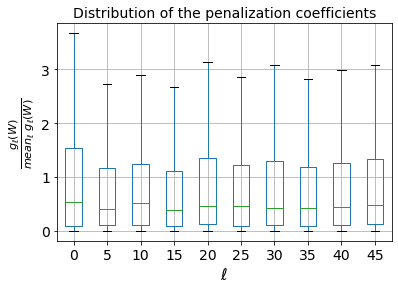
Figure 3: Distribution of $g_{l}(\bm{W})$ across the layers at initialization for Vanilla ResNet50 with width 512.

Lemma 2 shows that under fixed budget, the mode $\bm{p}^{*}$ that maximizes the regularization induced by $\mathcal{SD}$ is generally layer-dependent ($\neq$ uniform). However, we show that at initialization, on average (w.r.t $\bm{W}$), $\bm{p}^{*}$ is uniform.

Theorem 1 ($p^{*}$ is uniform at initialization).

Assume $\phi=\textrm{ReLU}$ and $\bm{W}$ are initialized with $\mathcal{N}(0,\frac{2}{N})$. Then, in the infinite width limit, under 1, for all $l\in[1:L]$, we have

$$\mathbb{E}_{\bm{W}}[g_{l}(\bm{W})]=\mathbb{E}_{\bm{W}}[g_{1}(\bm{W})].$$

As a result, given a budget $\bar{L}$, the average regularization term $\frac{1}{2L}\sum_{l=1}^{L}p_{l}(1-p_{l})\mathbb{E}_{\bm{W}}[g_{l}(\bm{W})]$ is maximal for the uniform mode $\bm{p}^{*}=(\bar{L}/L,\dots,\bar{L}/L)$.

The proof of 1 is based on some results from the signal propagation theory in deep neural network. We provide an overview of this theory in Appendix A0. 1 shows that, given a training budget $\bar{L}$ and a randomly initialized ResNet with $\mathcal{N}(0,2/N)$ and $N$ large, the average (w.r.t $\bm{W}$) maximal regularization at initialization is almost achieved by the uniform mode. This is because the coefficients $\mathbb{E}_{\bm{W}}[g_{l}(\bm{W})]$ are equal under 1, which we highlight in Fig. 3. As a result, we would intuitively expect that the uniform mode performs best when the budget $\bar{L}$ is large, e.g. $L$ is large and $\bar{L}\approx L$, since in this case, at each iteration, we update the weights of an overparameterized subnetwork, which would require more regularization compared to the small budget regime. We formalize this intuition in Section 5.

In the next section, we show that $\mathcal{SD}$ is linked to another regularization effect that only occurs in the large depth limit; in this limit, we show that $\mathcal{SD}$ mimics Gaussian Noise Injection methods by adding Gaussian noise to the pre-activations.

4.2 Stochastic Depth mimics Gaussian noise injection

Recent work by Camuto et al. [2020] studied the regularization effect of Gaussian Noise Injection (GNI) on the loss function and showed that adding isotropic Gaussian noise to the activations $z_{l}$ improves generalization by acting as a regularizer on the loss. The authors suggested adding a zero mean Gaussian noise parameterized by its variance. At training time $t$, this translates to replacing $z_{l}^{t}$ by $z_{l}^{t}+\mathcal{N}(0,\sigma_{l}^{2}I)$, where $z_{l}^{t}$ is the value of the activations in the $l^{th}$ layer at training time $t$, and $\sigma_{l}^{2}$ is a parameter that controls the noise level. Empirically, adding this noise tends to boost the performance by making the model robust to over-fitting. Using similar perturbation analysis as in the previous section, we show that when the depth is large, $\mathcal{SD}$ mimics GNI by implicitly adding a non-isotropic data-adaptive Gaussian noise to the pre-activations $y_{l}$ at each training iteration. We bring to the reader’s attention that the following analysis holds throughout the training (it is not limited to the initialization), and does not require the infinite-width regime.

Consider an arbitrary neuron $y^{i}_{\alpha L}$ in the $(\alpha L)^{th}$ layer for some fixed $\alpha\in(0,1)$. $y^{i}_{\alpha L}(x,\bm{\delta})$ can be approximated using a first order Taylor expansion around $\bm{\delta}=\bm{1}$. We obtain similarly,

$$\begin{split}y^{i}_{\alpha L}(x,\bm{\delta})&\approx\bar{y}^{i}_{\alpha L}(x)+\frac{1}{\sqrt{L}}\sum_{l=1}^{\alpha L}\eta_{l}\,\langle z_{l},\nabla_{y_{l}}G_{l}^{i}(y_{l}(x;\bm{1}))\rangle\end{split}$$ (7)

where $G_{l}^{i}$ is defined by $y^{i}_{\alpha L}(x;\bm{1})=G_{l}^{i}(y_{l}(x;\bm{1}))$, $\eta_{l}=\delta_{l}-p_{l}$, and $\bar{y}^{i}_{\alpha L}(x)=y^{i}_{\alpha L}(x,\bm{1})+\frac{1}{\sqrt{L}}\sum_{l=1}^{\alpha L}(p_{l}-1)\,\langle z_{l},\nabla_{y_{l}}G_{l}^{i}(y_{l}(x;\bm{1}))\rangle\approx y^{i}_{\alpha L}(x,\bm{p})$.

Let $\gamma_{\alpha,L}(x)=\frac{1}{\sqrt{L}}\sum_{l=1}^{\alpha L}\eta_{l}\,\langle z_{l},\nabla_{y_{l}}G_{l}^{i}(y_{l}(x;\bm{1}))\rangle$. With $\mathcal{SD}$, $y^{i}_{\alpha L}(x;\bm{\delta})$ can therefore be seen as a perturbed version of $y^{i}_{\alpha L}(x;\bm{p})$ (the pre-activation of the average network) with noise $\gamma_{\alpha,L}(x)$. The scaling factor $1/\sqrt{L}$ ensures that $\gamma_{\alpha,L}$ remains bounded (in $\ell_{2}$ norm) as $L$ grows. Without this scaling, the variance of $\gamma_{\alpha,L}$ will generally explode. The term $\gamma_{\alpha,L}$ captures the randomness of the binary mask $\bm{\delta}$, which up to a factor $\alpha$, resembles to the scaled mean in Central Limit Theorem(CLT) and can be written as $\gamma_{\alpha,L}(x)=\sqrt{\alpha}\times\frac{1}{\sqrt{\alpha L}}\sum_{l=2}^{\alpha L}X_{l,L}(x)$ where $X_{l,L}(x)=\eta_{l}\,\langle z_{l},\nabla_{y_{l}}G_{l}^{i}(y_{l}(x;\bm{1}))\rangle$. Ideally, we would like to apply CLT to conclude on the Gaussianity of $\gamma_{\alpha,L}(x)$ in the large depth limit. However, the random variables $X_{l}$ are generally not $i.i.d$ (they have different variances) and they also depend on $L$. Thus, standard CLT argument fails. Fortunately, there is a more general form of CLT known as Lindeberg’s CLT which we use in the proof of the next theorem.

Theorem 2.

Let $x\in\mathbb{R}^{d}$, $X_{l,L}(x)=\eta_{l}\,\mu_{l,L}(x)$ where $\mu_{l,L}(x)=\langle z_{l},\nabla_{y_{l}}G^{i}_{l}(y_{l}(x;\bm{1})\rangle$, and $\sigma_{l,L}^{2}(x)=\textrm{Var}_{\delta}[X_{l,L}(x)]=p_{l}(1-p_{l})\mu_{l,L}(x)^{2}$ for $l\in[L]$. Assume that

$1.$ There exists $a\in(0,1/2)$ such that for all $L$, and $l\in[L]$, $p_{l}\in(a,1-a)$.

$2.$ $\lim_{L\to\infty}\frac{\max_{k\in[L]}\mu_{k,L}^{2}(x)}{\sum_{l=1}^{L}\mu_{l,L}^{2}(x)}=0$.

$3.$ $v_{\alpha,\infty}(x):=\lim_{L\to\infty}\frac{\sum_{l=1}^{L}\sigma_{l,L}^{2}(x)}{L}$ exists and is finite.

Then,  $\gamma_{\alpha,L}(x)\underset{L\to\infty}{\overset{D}{\longrightarrow}}\mathcal{N}(0,\alpha\,v_{\alpha,\infty}(x)).$

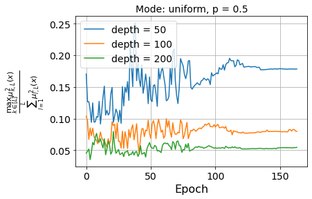
Figure 4: (2) Assumption 2 as a function the depth $L$ and epoch.

Fig. 4 provides an empirical verification of the second condition of 2 across all training epochs. There is a clear downtrend as the depth increases; this trend is consistent throughout training, which supports the validity of the second condition in 2 at all training times. 2 shows that training a ResNet with $\mathcal{SD}$ involves implicitly adding the noise $\gamma_{\alpha,L}(x)$ to $y^{i}_{\alpha L}$. This noise becomes asymptotically normally distributed, confirming that $\mathcal{SD}$ implicitly injects input-dependent Gaussian noise in this limit. Camuto et al. [2020] studied GNI in the context of input-independent noise and concluded on the benefit of such methods on the overall performance of the trained network. We empirically confirm the results of 2 in Section 6 using different statistical normality tests.

Similarly, we study the implicit regularization effect of $\mathcal{SD}$ induced on the gradient in Appendix A3, and show that under some assumptions, $\mathcal{SD}$ acts implicitly on the gradient by adding Gaussian noise in the large depth limit.

5 The Budget Hypothesis

We have seen in Section 4 that given a budget $\bar{L}$, the uniform mode is linked to maximal regularization with $\mathcal{SD}$ at initialization (1). Intuitively, for fixed weights $\bm{W}$, the magnitude of standard regularization methods such as $\|.\|_{1}$ or $\|.\|_{2}$ correlates with the number of parameters; the larger the model, the bigger the penalization term. Hence, in our case, we would require the regularization term to correlate (in magnitude) with the number of parameters, or equivalently, the number of trainable layers. Assuming $L\gg 1$, and given a fixed budget $\bar{L}$, the number of trainable layers at each training iteration is close to $\bar{L}$ (Lemma 1). Hence, the magnitude of the regularization term should depend on how large/small the budget $\bar{L}$ is, as compared to $L$.

Small budget regime ($\bar{L}/L\ll 1$).

In this regime, the effective depth $L_{\bm{\delta}}$ of the subnetwork is small compared to $L$. As the ratio $\bar{L}/L$ gets smaller, the sampled subnetworks become shallower, suggesting that the regularization need not be maximal in this case, and therefore $\bm{p}$ should not be uniform in accordance with 1. Another way to look at this is through the bias-variance trade-off principle. Indeed, as $\bar{L}/L\to 0$, the variance of the model decreases (and the bias increases), suggesting less regularization is needed. The increase in bias inevitably causes a deterioration of the performance; we call this the Budget-performance trade-off. To derive a more sensible choice of $\bm{p}$ for small budget regimes, we introduce a new Information Discrepancy based algorithm (Section 4). We call this algorithm Sensitivity Mode or briefly SenseMode. This algorithm works in two steps:

1. Compute the sensitivity ($\mathcal{S}$) of the loss w.r.t the layer at initialization using the approximation,

   $$\mathcal{S}_{l}=\mathcal{L}(\bm{W};\bm{1})-\mathcal{L}(\bm{W};\bm{1}_{l})\approx\nabla_{\delta_{l}}\mathcal{L}(\bm{W};\bm{\delta})_{|\bm{\delta}=\bm{1}}.$$

   $\mathcal{S}_{l}$ is a measure of the sensitivity of the loss to keeping/removing the $l^{th}$ layer.

2. Use a mapping $\varphi$ to map $\mathcal{S}$ to the mode, $\bm{p}=\varphi(\mathcal{S})$, where $\varphi$ is a linear mapping from the range of $S$ to $[p_{min},1]$ and $p_{min}$ is the minimum survival rate (fixed by the user).

Large budget regime ($\bar{L}/L\sim 1$).

In this regime, the effective depth $L_{\bm{\delta}}$ of the subnetworks is close to $L$, and thus, we are in the overparameterized regime where maximal regularization could boost the performance of the model by avoiding over-fitting. Thus, we anticipate the uniform mode to perform better than other alternatives in this case. We are now ready to formally state our hypothesis,

Budget hypothesis.

Assuming $L\gg 1$, the uniform mode outperforms SenseMode in the large budget regime, while SenseMode outperforms the uniform mode in the small budget regime.

We empirically validate the Budget hypothesis and the Budget-performance trade-off in Section 6.

6 Experiments

The objective of this section is two-fold: we empirically verify the theoretical analysis developed in sections 3 and 4 with a Vanilla ResNet model on a toy regression task; we also empirically validate the Budget Hypothesis on the benchmark datasets CIFAR-10 and CIFAR-100 [Krizhevsky et al., 2009]. Notebooks and code to reproduce all experiments, plots and tables presented are available in the supplementary material. We perform comparisons at constant training budgets.

Implementation details:

Vanilla Stable ResNet is composed of identical residual blocks each formed of a Linear layer followed by ReLU. Stable ResNet110 follows [He et al., 2016, Huang et al., 2016]; it comprises three groups of residual blocks; each block consists of a sequence Convolution-BatchNorm-ReLU-Convolution-BatchNorm. We build on an open-source implementation of standard ResNet. We scale the blocks using a factor $1/\sqrt{L}$ as described in Section 3. The toy regression task consists of estimating the function $f_{\beta}:x\mapsto\sin(\beta^{T}x),$ where the inputs $x$ and parameter $\beta$ are in $\mathbb{R}^{256}$, sampled from a standard Gaussian. CIFAR-10, CIFAR-100 contain 32-by-32 color images, representing respectively 10 and 100 classes of natural scene objects. We present here our main conclusions. Further implementation details and other insightful results are in the Appendix A4.

Gaussian Noise Injection:

We proceed by empirically verifying the Gaussian behavior of the neurons as described in 4. For each input $x$, we sample 200 masks and the corresponding $y(x;\bm{\delta})$. We then compute the p-value $pv_{x}$ of the Shapiro-Wilk test of normality [Shapiro and Wilk, 1965]. In Fig. 5 we represent the distribution of the p-values $\{pv_{x}\ |\ x\in\mathcal{X}\}$. We can see that the Gaussian behavior holds throughout training (left). On the right part of the Figure, we can see that the Normal behavior becomes accurate after approximately 20 layers. In the Appendix we report further experiments with different modes, survival rates, and a different test of normality to verify both 2 and the critical assumption 2.

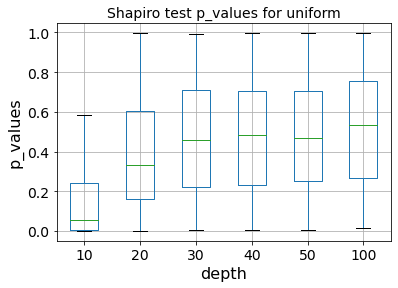
Figure 5: Empirical verification of Theorem 2 on Vanilla ResNet100 with width 128 with average survival probability $\bar{L}/L=0.7$ and uniform mode. Distribution of the p-values for Shapiro’s normality test as a function of the training epoch (left) and depth of the network (right).

Empirical verification of the Budget Hypothesis:

We compare the three modes: Uniform, Linear, and SenseMode on two benchmark datasets using a grid survival proportions. The values and standard deviations reported are obtained using four runs. For SenseMode, we use the simple rule $p_{l}\propto|\mathcal{S}_{l}|$, where $\mathcal{S}_{l}$ is the sensitivity (see section 5). We report in Table 2(b) the results for Stable ResNet110. Results with Stable ResNet56 are reported in Appendix A4.

Table 2: Comparison of the modes of selection of the survival probabilities with fixed budget with Stable ResNet110.

$\bar{L}/L$	Uniform	SenseMode	Linear
0.1	17.2 $\pm$ 0.3	15.4 $\pm$ 0.4	$-$
0.2	10.3 $\pm$ 0.4	9.3 $\pm$ 0.5	$-$
0.3	7.7 $\pm$ 0.2	7.0 $\pm$ 0.3	$-$
0.4	7.4 $\pm$ 0.3	7.3 $\pm$ 0.4	$-$
0.5	6.8 $\pm 0.1$	7.3 $\pm$ 0.2	9.1 $\pm$ 0.1
0.6	6.3 $\pm 0.2$	6.9 $\pm$ 0.1	7.5 $\pm$ 0.2
0.7	5.9 $\pm$ 0.1	7.3 $\pm$ 0.3	6.4 $\pm$ 0.2
0.8	5.7 $\pm$ 0.1	6.6 $\pm$ 0.2	6.1 $\pm$ 0.2
0.9	5.7 $\pm$ 0.1	6.2 $\pm$ 0.2	6.0 $\pm$ 0.2
1	$6.37\pm 0.12$

(a) CIFAR10

$\bar{L}/L$	Uniform	SenseMode	Linear
0.1	55.2 $\pm$ 0.4	51.3 $\pm$ 0.6	$-$
0.2	38.3 $\pm$ 0.3	36.4 $\pm$ 0.4	$-$
0.3	31.4 $\pm$ 0.2	30.1 $\pm$ 0.5	$-$
0.4	30.9 $\pm$ 0.2	28.5 $\pm$ 0.4	$-$
0.5	28.4 $\pm$ 0.3	29.5 $\pm$ 0.5	36.5 $\pm$ 0.4
0.6	26.5 $\pm$ 0.4	29.9 $\pm$ 0.6	30.9 $\pm$ 0.4
0.7	25.8 $\pm$ 0.1	29.5 $\pm$ 0.3	27.3 $\pm$ 0.3
0.8	25.5 $\pm$ 0.1	30.0 $\pm$ 0.3	25.7 $\pm$ 0.2
0.9	25.5 $\pm$ 0.3	28.3 $\pm$ 0.2	25.5 $\pm$ 0.2
1	26.5 $\pm$ 0.2

(b) CIFAR100

The empirical results are coherent with the Budget Hypothesis. When the training budget is large, i.e. $\bar{L}/L\geq 0.5$, the Uniform mode outperforms the others. We note nevertheless that when $\bar{L}/L\geq 0.9$, the Linear and Uniform models have similar performance. This seems reasonable as the Uniform and Linear probabilities become very close for such survival proportions. When the budget is low, i.e. $\bar{L}/L<0.5$, the SenseMode outperforms the uniform one (the linear mode cannot be used with budgets $\bar{L}<L/2$ when $L\gg 1$, since $\sum p_{l}/L>1/2-1/(2L)\sim 1/2$), thus confirming the Budget hypothesis. Table 2(b) also shows a clear Budget-performance trade-off.

7 Related work

The regularization effect of Dropout in the context of linear models has been the topic of a stream of papers [Wager et al., 2013, Mianjy and Arora, 2019, Helmbold and Long, 2015, Cavazza et al., 2017]. This analysis has been recently extended to neural networks by Wei et al. [2020] where authors used a similar approach to ours to depict the explicit and implicit regularization effects of Dropout. To the best of our knowledge, our paper is the first to provide analytical results for the regularization effect of $\mathcal{SD}$, and study the large depth behaviour of $\mathcal{SD}$, showing that the latter mimics Gaussian Noise Injection [Camuto et al., 2020]. A further analysis of the implicit regularization effect of $\mathcal{SD}$ is provided in Appendix A3.

8 Limitations and extensions

In this work, we provided an analytical study of the regularization effect of $\mathcal{SD}$ using a second order Taylor approximation of the loss function. Although the remaining higher order terms are usually dominated by the second order approximation (See the quality of the second order approximation in Appendix A4), they might also be responsible for other regularization effects. This is a common limitation in the literature on noise-based regularization in deep neural networks [Camuto et al., 2020, Wei et al., 2020]. Further research is needed to isolate the effect of higher order terms.
We also believe that SenseMode opens an exciting research direction knowing that the low budget regime has not been much explored yet in the literature. We believe that one can probably get even better results with more elaborate maps $\varphi$ such that $\bm{p}=\varphi(\mathcal{S})$. Another interesting extension of an algorithmic nature is the dynamic use of SenseMode throughout training. We are currently investigating this topic which we leave for future work.

Appendix

A0 An overview of signal propagation in wide neural networks

In section, we review some results and tools from the theory of signal of propagation in wide neural networks. This will prove valuable in the rest of the appendix.

A0.1 Neural Network Gaussian Process (NNGP)

Standard ResNet without $\mathcal{SD}$.

Consider a standard ResNet architecture with $L$ layers. The forward propagation of some input $x\in\mathbb{R}^{d}$ is given by

$$y_{0}(x) =\Psi_{0}(x,W_{0})$$ (A1)

$$y_{l}(x) =y_{l-1}(x)+\Psi_{l}(y_{l-1}(x),W_{l}),\quad 1\leq l\leq L,$$

$$y_{out}(x) =\Psi_{out}(y_{L}(x),W_{out}),$$

where $W_{l}$ are the weights in the $l^{th}$ layer, $\Psi$ is a mapping that defines the nature of the layer, and $y_{l}$ are the pre-activations. we consider constant width ResNet and we further denote by $N$ the width, i.e. for all $l\in[L-1]$, $y_{l}\in\mathbb{R}^{N}$. The output function of the network is given by $s(y_{out})$ where $s$ is some convenient mapping for the learning task, e.g. the Softmax mapping for classification tasks. We denote by $o$ the dimension of the network output, i.e. $s(y_{out})\in\mathbb{R}^{o}$ which is also the dimension of $y_{out}$. For our theoretical analysis, we consider residual blocks composed of a Fully Connected linear layer

$$\Psi_{l}(x,W)=W\phi(x).$$

where $\phi(x)$ is the activation function. The weights are initialized with He init He et al. [2015], e.g. for ReLU, $W^{l}_{ij}\sim\mathcal{N}(0,2/N)$.

The neurons $\{y_{0}^{i}(x)\}_{i\in[1:N]}$ are iid normally distributed random variables since the weights connecting them to the inputs are iid normally distributed. Using the Central Limit Theorem, as $N_{0}\rightarrow\infty$, $y^{i}_{1}(x)$ becomes a Gaussian variable for any input $x$ and index $i\in[1:N]$. Additionally, the variables $\{y^{i}_{1}(x)\}_{i\in[1:N]}$ are iid. Thus, the processes $y^{i}_{1}(.)$ can be seen as independent (across $i$) centred Gaussian processes with covariance kernel $Q_{1}$. This is an idealized version of the true process corresponding to letting width $N_{0}\to\infty$. Doing this recursively over $l$ leads to similar results for $y_{l}^{i}(.)$ where $l\in[1:L]$, and we write accordingly $y_{l}^{i}\stackrel{{\scriptstyle ind}}{{\sim}}\mathcal{GP}(0,Q_{l})$. The approximation of $y_{l}^{i}(.)$ with a Gaussian process was first proposed by [Neal, 1995] for single layer FeedForward neural networks and was extended recently to multiple feedforward layers by [Lee et al., 2019] and [Matthews et al., 2018]. More recently, excellent work by [Yang, 2020] introduced a unifying framework named Tensor Programs, confirming the large-width Gaussian Process behaviour for nearly all neural network architectures.

For any input $x\in\mathbb{R}^{d}$, we have $\mathbb{E}[y^{i}_{l}(x)]=0$, so that the covariance kernel is given by $Q_{l}(x,x^{\prime})=\mathbb{E}[y_{l}^{1}(x)y_{l}^{1}(x^{\prime})]$. It is possible to evaluate the covariance kernels layer by layer, recursively. More precisely, assume that $y_{l-1}^{i}$ is a Gaussian process for all $i$. Let $x,x^{\prime}\in\mathbb{R}^{d}$. We have that

$$Q_{l}(x,x^{\prime}) =\mathbb{E}[y_{l}^{1}(x)y_{l}^{1}(x^{\prime})]$$

$$=\mathbb{E}[y_{l-1}^{1}(x)y_{l-1}^{1}(x^{\prime})]+\sum_{j=1}^{N_{l-1}}\mathbb{E}[(W_{l}^{1j})^{2}\phi(y^{j}_{l-1}(x))\phi(y^{j}_{l-1}(x^{\prime}))]$$

$$+\mathbb{E}\left[\sum_{j=1}^{N_{l-1}}W_{l}^{1j}(y_{l-1}^{1}(x)\phi(y_{l-1}^{1}(x^{\prime}))+y_{l-1}^{1}(x^{\prime})\phi(y_{l-1}^{1}(x)))\right].$$

Some terms vanish because $\mathbb{E}[W_{l}^{1j}]=0$. Let $Z_{j}=\sqrt{\frac{N}{2}W_{l}^{1j}}$. The second term can be written as

$$\mathbb{E}\left[\frac{2}{N}\sum_{j}(Z_{j})^{2}\phi(y^{j}_{l-1}(x))\phi(y^{j}_{l-1}(x^{\prime}))\right]\rightarrow 2\,\mathbb{E}[\phi(y^{1}_{l-1}(x))\phi(y^{1}_{l-1}(x^{\prime}))]\,,$$

where we have used the Central Limit Theorem. Therefore, the kernel $Q_{l}$ satisfies for all $x,x^{\prime}\in\mathbb{R}^{d}$

$$Q_{l}(x,x^{\prime}) =Q_{l-1}(x,x^{\prime})+\mathcal{F}_{l-1}(x,x^{\prime})\,,$$

where $\mathcal{F}_{l-1}(x,x^{\prime})=2\,\mathbb{E}[\phi(y_{l-1}^{1}(x))\phi(y_{l-1}^{1}(x^{\prime}))]$.

For the ReLU activation function $\phi:x\mapsto\max(0,x)$, the recurrence can be written more explicitly as in [Hayou et al., 2019]. Let $C_{l}$ be the correlation kernel, defined as

$$C_{l}(x,x^{\prime})=\tfrac{Q_{l}(x,x^{\prime})}{\sqrt{Q_{l}(x,x)Q_{l}(x^{\prime},x^{\prime})}}$$ (A2)

and let $f:[-1,1]\to\mathbb{R}$ be given by

$$f:\gamma\mapsto\tfrac{1}{\pi}(\sqrt{1-\gamma^{2}}+\gamma\arcsin\gamma)+\frac{1}{2}\gamma\,.$$ (A3)

The recurrence relation reads

$$\begin{split}&Q_{l}=Q_{l-1}+\tfrac{f(C_{l-1})}{C_{l-1}}Q_{l-1}\,,\\ &Q_{0}(x,x^{\prime})=2\,\tfrac{x\cdot x^{\prime}}{d}\,.\end{split}$$ (A4)

Standard ResNet with $\mathcal{SD}$.

The introduction of the binary mask $\bm{\delta}$ in front of the residual blocks slightly changes the recursive expression of the kernel $Q_{l}$. It ii easy to see that with $\mathcal{SD}$, the $Q_{l}$ follows

$$\begin{split}&Q_{l}=Q_{l-1}+p_{l}\tfrac{f(C_{l-1})}{C_{l-1}}Q_{l-1}\,,\\ &Q_{0}(x,x^{\prime})=2\,\tfrac{x\cdot x^{\prime}}{d}\,.\end{split}$$ (A5)

where $f$ is given by Eq. A3.

We obtain similar formulas for Stable ResNet with and without $\mathcal{SD}$.

Stable ResNet without $\mathcal{SD}$.

$$\begin{split}&Q_{l}=Q_{l-1}+\frac{1}{L}\tfrac{f(C_{l-1})}{C_{l-1}}Q_{l-1}\,,\\ &Q_{0}(x,x^{\prime})=2\,\tfrac{x\cdot x^{\prime}}{d}\,.\end{split}$$ (A6)

Stable ResNet with $\mathcal{SD}$.

$$\begin{split}&Q_{l}=Q_{l-1}+\frac{p_{l}}{L}\tfrac{f(C_{l-1})}{C_{l-1}}Q_{l-1}\,,\\ &Q_{0}(x,x^{\prime})=2\,\tfrac{x\cdot x^{\prime}}{d}\,.\end{split}$$ (A7)

A0.2 Diagonal elements of the kernel $Q_{l}$

Lemma A1 (Diagonal elements of the covariance).

Consider a ResNet of the form Eq. 1 (standard ResNet) or Eq. 3(Stable ResNet), and let $x\in\mathbb{R}^{d}$. We have that for all $l\in[1:L]$,

• Standard ResNet without $\mathcal{SD}$: $Q_{l}(x,x)=2^{l}Q_{0}(x,x)\,.$

• Standard ResNet with $\mathcal{SD}$: $Q_{l}(x,x)=\prod_{k=1}^{l}(1+p_{k})Q_{0}(x,x)\,.$

• Stable ResNet without $\mathcal{SD}$: $Q_{l}(x,x)=(1+\frac{1}{L})^{l}Q_{0}(x,x)\,.$

• Stable ResNet with $\mathcal{SD}$: $Q_{l}(x,x)=\prod_{k=1}^{l}(1+\frac{p_{k}}{L})Q_{0}(x,x)\,.$

Proof.

Let us prove the result for Standard ResNet with $\mathcal{SD}$. The proof is similar for the other cases. Let $x\in\mathbb{R}^{d}$. We know that

$$Q_{l}(x,x)=Q_{l-1}(x,x)+p_{l}f(1)Q_{l-1}(x,x)\,,$$

where $f$ is given by Eq. A3. It is straightforward that $f(1)=1$. This yields

$$Q_{l}(x,x)=(1+p_{l})Q_{l-1}(x,x)\,.$$

we conclude by telescopic product. ∎

A0.3 1 and gradient backpropagation

For gradient back-propagation, an essential assumption in the literature on signal propagation analysis in deep neural networks is that of the gradient independence which is similar in nature to the practice of feedback alignment [Lillicrap et al., 2016]. This assumption (1) allows for derivation of recursive formulas for gradient back-propagation, and it has been extensively used in literature and empirically verified; see references below.

Gradient Covariance back-propagation.

1 was used to derive analytical formulas for gradient covariance back-propagation in a stream of papers; to cite a few, [Hayou et al., 2019, samuellee_gaussian_process, Poole et al., 2016, Xiao et al., 2018, Yang and Schoenholz, 2017]. It was validated empirically through extensive simulations that it is an excellent tool for FeedForward neural networks in Schoenholz et al. [2017], for ResNets in Yang and Schoenholz [2017] and for CNN in Xiao et al. [2018].

Neural Tangent Kernel (NTK).

1 was implicitly used by Jacot et al. [2018] to derive the recursive formula of the infinite width Neural Tangent Kernel (See Jacot et al. [2018], Appendix A.1). Authors have found that this assumption yields excellent empirical match with the exact NTK. It was also used later in [Arora et al., 2019, Hayou et al., 2020] to derive the infinite depth NTK for different architectures.

When used for the computation of gradient covariance and Neural Tangent Kernel, [Yang, 2020] proved that 1 yields the exact computation of the gradient covariance and the NTK in the limit of infinite width. We state the result for the gradient covariance formally.

Lemma A2 (Corollary of Theorem D.1. in [Yang, 2020]).

Consider a ResNet of the form (1) or (3) with weights $W$. In the limit of infinite width, we can assume that $W^{T}$ used in back-propagation is independent from $W$ used for forward propagation, for the calculation of Gradient Covariance.

Lemma A3 (Gradient Second moment).

Consider a ResNet of type Eq. 3 without $\mathcal{SD}$. Let $(x,t)\in\mathcal{D}$ be a sample from the dataset, and define the second of the gradient with $\tilde{q}_{l}(x,t)=\mathbb{E}_{\bm{W}}\left[\frac{\partial\mathcal{L}(x,\bm{W})}{\partial y_{l}}\right]$. Then, in the limit of infinite width, we have that

$$\tilde{q}^{l}(x,t)=\left(1+\frac{1}{L}\right)\,\tilde{q}^{l+1}(x,t)\,.$$

As a result, for all $l\in[1:L]$, we have that

$$\tilde{q}^{l}(x,t)=\left(1+\frac{1}{L}\right)^{L-l}\,\tilde{q}^{L}(x,t)\,.$$

Proof.

It is straighforward that

$$\frac{\partial\mathcal{L}(x,\bm{W})}{\partial y_{l}^{i}}=\frac{\partial\mathcal{L}(x,\bm{W})}{\partial y_{l+1}^{i}}+\frac{1}{\sqrt{L}}\sum_{j}\frac{\partial\mathcal{L}(x,\bm{W})}{\partial y_{l+1}^{j}}W_{l+1}^{ji}\phi^{\prime}(y_{l}^{i}(x))\,.$$

Using lemma A2 and the Central Limit Theorem, we obtain

$$\tilde{q}^{l}(x,t)=\tilde{q}^{l+1}(x,t)+\frac{2}{L}\tilde{q}^{l+1}(x,t)\mathbb{E}[\phi^{\prime}(y_{l}^{1}(x))^{2}]\,.$$

We conclude by observing that $\mathbb{E}[\phi^{\prime}(y^{l}_{i}(x))^{2}]=\mathbb{P}(\mathcal{N}(0,1)>0)=\frac{1}{2}$. ∎

A1 Proofs

A1.1 Proof of Lemma 1

Lemma 1 (Concentration of $L_{\bm{\delta}}$).

For any $\beta\in(0,1)$, we have that with probability at least $1-\beta$,

$$|L_{\bm{\delta}}-L_{\bm{p}}|\leq v_{\bm{p}}\,u^{-1}\left(\frac{\log(2/\beta)}{v_{\bm{p}}}\right)$$ (A8)

where $L_{\bm{p}}=\mathbb{E}[L_{\bm{\delta}}]=\sum_{l=1}^{L}p_{l}$, $v_{\bm{p}}=\textup{Var}[L_{\bm{\delta}}]=\sum_{l=1}^{L}p_{l}(1-p_{l})$, and $u(t)=(1+t)\log(1+t)-t$.

Moreover, for a given average depth $L_{\bm{p}}=\bar{L}$, the upperbound in Eq. 2 is maximal for the uniform choice of survival probabilities $\bm{p}=\left(\frac{\bar{L}}{L},...,\frac{\bar{L}}{L}\right)$.

Proof.

The concentration inequality is a simple application of Bennett’s inequality: Let $X_{1},...,X_{n}$ be a sequence of independent random variables with finite variance and zero mean. Assume that there exists $a\in\mathbb{R}^{+}$ such that $X_{i}\leq a$ almost surely for all $i$. Define $S_{n}=\sum_{i=1}^{n}X_{i}$ and $\sigma_{n}^{2}=\sum_{i=1}^{n}\mathbb{E}[X_{i}^{2}]$. Then, for any $t>0$, we have that

$$\mathbb{P}(|S_{n}|>t)\leq 2\exp\left(-\frac{\sigma_{n}^{2}}{a^{2}}u\left(\frac{at}{\sigma_{n}^{2}}\right)\right).$$

Now let us prove the second result. Fix some $\bar{L}\in(0,L)$. We start by proving that the function $\zeta(z)=z\,u^{-1}\left(\frac{\alpha}{z}\right)$ is increasing for any fixed $\alpha>0$. Observe that $u^{\prime}(t)=\log(1+t)$, so that

$$(u^{-1})^{\prime}(z)=\frac{1}{u^{\prime}(u^{-1}(z))}=\frac{1+u^{-1}(z)}{z+u^{-1}(z)}.$$

This yields

$$\zeta^{\prime}(z)=\frac{zu^{-1}\left(\frac{\alpha}{z}\right)^{2}-\alpha}{\alpha+xu^{-1}\left(\frac{\alpha}{z}\right)}$$

For $z>0$, the numerator is positive if and only if $\frac{\alpha}{z}>u\left(\sqrt{\frac{\alpha}{z}}\right)$, which is always true using the inequality $\log(1+t)<t$ for all $t>0$.

Now let $\alpha=\log(2/\beta)$. Without restrictions on $L_{\bm{p}}$, it is straightforward that $v_{\bm{p}}$ is maximized by $\bm{p}^{\prime}=(1/2,...,1/2)$. With the restriction $L_{\bm{p}}=\bar{L}$, the minimizer is the orthogonal projection of $\bm{p}^{\prime}$ onto the convex set $\{\bm{p}:L_{\bm{p}}=\bar{L}\}$. This projection inherits the symmetry of $\bm{p}^{\prime}$, which concludes the proof. ∎

A1.2 Proof of 1

Theorem 1 (Exploding gradient rate).

Let $\mathcal{L}(x,z)=\ell(y_{out}(x;\bm{\delta}),z)$ for $(x,z)\in\mathbb{R}^{d}\times\mathbb{R}^{o}$, where $\ell(z,z^{\prime})$ is some differentiable loss function. Let $\tilde{q}_{l}(x,z)=\mathbb{E}_{W,\bm{\delta}}\frac{\lVert\nabla_{y_{l}}\mathcal{L}\rVert^{2}}{\lVert\nabla_{y_{L}}\mathcal{L}\rVert^{2}}$, where the numerator and denominator are respectively the norms of the gradients with respect to the inputs of the $l^{th}$ and $L^{th}$ layers . Then, in the infinite width limit, under 1, for all $l\in[L]$ and $(x,z)\in\mathbb{R}^{d}\times\mathbb{R}^{o}$, we have

• With Stochastic Depth, $\tilde{q}_{l}(x,z)=\prod_{k=l+1}^{L}(1+p_{k})$

• Without Stochastic Depth (i.e. $\bm{\delta}=\bm{1}$), $\tilde{q}_{l}(x,z)=2^{L-l}$

Proof.

It is straightforward that with Stochastic Depth

$$\frac{\partial\mathcal{L}(x,\bm{W})}{\partial y_{l}^{i}}=\frac{\partial\mathcal{L}(x,\bm{W})}{\partial y_{l+1}^{i}}+\delta_{l+1}\sum_{j}\frac{\partial\mathcal{L}(x,\bm{W})}{\partial y_{l+1}^{j}}W_{l+1}^{ji}\phi^{\prime}(y_{l}^{i}(x))\,.$$

Denote for clarity for any neuron $i$ and layer $l$, $d_{i,l}=\frac{\partial\mathcal{L}(x,\bm{W})}{\partial y_{l}^{i}}.$ The equation can be written

$$d_{i,l}=d_{i,l+1}+\delta_{l+1}\sum\limits_{j}d_{j,l+1}W^{ji}_{l+1}\phi^{\prime}(y^{i}_{l}(x))$$ (A9)

We notice that for any $k\geq l+1$ and any $i$, $d_{i,k}$ on depends on $W_{l+1}$ through the forward pass, and that the terms $W^{ji}_{l+1}$ in equation (A9) come from the backward pass. Therefore, Lemma A2 entails

$$\mathbb{E}_{W^{\text{backward}}_{l+1}}\frac{\lVert\nabla_{y_{l}}\mathcal{L}\rVert^{2}}{\lVert\nabla_{y_{L}}\mathcal{L}\rVert^{2}} = \frac{\sum_{i}d_{i,l+1}^{2}+\delta_{l+1}^{2}\frac{2}{N}\sum_{i}\phi^{\prime}(y_{l}^{i}(x))^{2}\sum_{j}d_{j,l+1}^{2}}{\sum_{j}d_{j,L}^{2}}$$

$$= \frac{\lVert\nabla_{y_{l+1}}\mathcal{L}\rVert^{2}}{\lVert\nabla_{y_{L}}\mathcal{L}\rVert^{2}}(1+\delta_{l+1}\frac{2}{N}\sum_{i}\phi^{\prime}(y_{l}^{i}(x))^{2}),$$

where $\frac{2}{N}$ is the variance of $W^{ji}_{l+1}$ ($N$ is the width of the network). Again using Lemma A2 and taking the expectation with respect to the remaining weights and mask concludes the proof.

∎

A1.3 Proof of Lemma 2

Lemma 2 (Maximal regularization).

Consider the empirical loss $\mathcal{L}$ given by Eq. 6 for some fixed weights $\bm{W}$ (e.g. $\bm{W}$ could be the weights at any training step of SGD).Then, for a fixed training budget $\bar{L}$, the regularization is maximal for

$$p^{*}_{l}=\min\big{(}1,\max(0,\frac{1}{2}-Cg_{l}(\bm{W})^{-1})\big{)},$$

where $C$ is a normalizing constant, that has the same sign as $L-2\bar{L}$. The global maximum is obtained for $p_{l}=1/2$.

Proof.

Let $a_{l}=g_{l}(\bm{W})$. Noticing that $p_{l}(1-p_{l})=1/4-(p_{l}-1/2)^{2}$, it comes that

$$\sum\limits_{l}p_{l}(1-p_{l})a_{l} = \frac{\sum a_{l}}{4}-\sum_{l}(p_{l}-1/2)^{2}a_{l}$$

$$= \frac{\sum a_{l}}{4}-\left\|p\odot\sqrt{a}-\frac{\sqrt{a}}{2}\right\|_{2}^{2},$$

with the abuse of notations $\sqrt{a}=(\sqrt{a_{1}},...,\sqrt{a_{L}})$ and where $\odot$ stands for the element-wise product. We deduce from this expression that $p=\bm{\frac{1}{2}}$ is the global maximizer of the regularization term. With a fixed training budget, notice that the expression is maximal for $p^{*}\odot\sqrt{a}$ the orthogonal projection of $\frac{\sqrt{a}}{2}$ on the intersection of the affine hyper-plane $\mathcal{H}$ containing the $L$ points of the form $(0,...,L_{m}\sqrt{a_{l}},...,0)$ and the hyper-cube $\mathcal{C}$ of the points with coordinates in $[0,1]$. Writing the KKT conditions yields for every $l$:

$$p_{l}=1/2-\beta a_{l}^{-1}-\lambda_{0,l}\mathbb{1}_{p_{l}=0}+\lambda_{1,l}\mathbb{1}_{p_{l}=1},$$

where $\lambda_{0,l},\lambda_{1,l}\geq 0.$ Taking $p=p^{*}$, $\beta=C$, $\lambda_{0,l}=1/2+\beta a_{l}^{-1}$ and $\lambda_{1,l}=1/2-\beta a_{l}^{-1}.$ Since the program is quadratic, the KKT conditions are necessary and sufficient conditions, which concludes the proof.

∎

A1.4 Proof of 1

Theorem 1 ($p^{*}$ is uniform at initialization).

Assume $\phi=\textrm{ReLU}$ and $\bm{W}$ are initialized with $\mathcal{N}(0,\frac{2}{N})$. Then, in the infinite width limit, under 1, for all $l\in[1:L]$, we have

$$\mathbb{E}_{\bm{W}}[g_{l}(\bm{W})]=\mathbb{E}_{\bm{W}}[g_{1}(\bm{W})].$$

As a result, given a budget $\bar{L}$, the average regularization term $\frac{1}{2L}\sum_{l=1}^{L}p_{l}(1-p_{l})\mathbb{E}_{\bm{W}}[g_{l}(\bm{W})]$ is maximal for the uniform mode $\bm{p}^{*}=(\bar{L}/L,\dots,\bar{L}/L)$.

Proof.

Using the expression of $g_{l}$, we have that

$$\mathbb{E}_{\bm{W}}[g_{l}(\bm{W})]=\frac{2}{n}\sum_{i=1}^{n}\mathbb{E}_{\bm{W}}[\|\zeta_{l}(x_{i},\bm{W})\|_{2}^{2}].$$

Thus, to conclude, it is sufficient to show that for some arbitrary $i\in[1:n]$, we have $\mathbb{E}_{\bm{W}}[\|\zeta_{l}(x_{i},\bm{W})\|_{2}^{2}]=\mathbb{E}_{\bm{W}}[\|\zeta_{1}(x_{i},\bm{W})\|_{2}^{2}]$ for all $l\in[1,L]$.
Fix $i\in[1:n]$ and $l\in[1:L]$. For the sake of simplicity, let $z_{l}=z_{l}(x;\bm{1})$ and $y_{l}=y_{l}(x;\bm{1})$. We have that

$$\|\zeta_{l}(x,\bm{W})\|_{2}^{2}=\sum_{j=1}^{o}\langle\nabla_{y_{l}}G_{l}^{j}(y_{l}),z_{l}\rangle^{2}$$

Now let $j\in[1:o]$. We have that

$$\langle\nabla_{y_{l}}G_{l}^{j}(y_{l}),z_{l}\rangle^{2}=\sum_{k,k^{\prime}}\frac{\partial G_{l}^{j}}{\partial y_{l}^{k}}z_{l}^{k}\frac{\partial G_{l}^{j}}{\partial y_{l}^{k^{\prime}}}z_{l}^{k^{\prime}}$$

Using 1, in the limit $N\rightarrow\infty$, we obtain

$$\mathbb{E}_{\bm{W}}[\langle\nabla_{y_{l}}G_{l}^{j}(y_{l}),z_{l}\rangle^{2}]=\sum_{k,k^{\prime}}\mathbb{E}_{\bm{W}}\left[\frac{\partial G_{l}^{j}}{\partial y_{l}^{k}}\frac{\partial G_{l}^{j}}{\partial y_{l}^{k^{\prime}}}\right]\mathbb{E}_{\bm{W}}[z_{l}^{k}z_{l}^{k^{\prime}}]$$

Since $\mathbb{E}_{\bm{W}}[z_{l}^{k}z_{l}^{k^{\prime}}]=0$ for $k\neq k^{\prime}$, we have that

$$\mathbb{E}_{\bm{W}}[\langle\nabla_{y_{l}}G_{l}^{j}(y_{l}),z_{l}\rangle^{2}]=\sum_{k=1}^{\infty}\mathbb{E}_{\bm{W}}\left[\left(\frac{\partial G_{l}^{j}}{\partial y_{l}^{k}}\right)^{2}\right]\mathbb{E}_{\bm{W}}[(z_{l}^{k})^{2}]$$

Let us deal first with the term $\mathbb{E}_{\bm{W}}[(z_{l}^{k})^{2}]$.

Let $k\in\mathbb{N}$. Recall that for finite $N$, we have that $z_{l}^{k}=\sum_{m=1}^{N}W_{l}^{k,m}\phi(y_{l-1}^{m})$ and $W_{l}^{k,m}\sim\mathcal{N}(0,\frac{2}{N})$. Thus, using the Central Limit Theorem in the limit $N\rightarrow\infty$, we obtain

$$\mathbb{E}_{\bm{W}}[(z_{l}^{k})^{2}]=2\,\mathbb{E}_{Z\sim\mathcal{N}(0,1)}[\phi(\sqrt{q_{l-1}}Z)^{2}]=Q_{l-1}(x,x),$$

where $Q_{l-1}(x,x)$ is given by Lemma A1. We obtain

$$\mathbb{E}_{\bm{W}}[(z_{l}^{k})^{2}]=\left(1+\frac{1}{L}\right)^{l-1}Q_{0}(x,x).$$

The term $\bar{q}^{j}_{l}=\mathbb{E}_{\bm{W}}\left[\left(\frac{\partial G_{l}^{j}}{\partial y_{l}^{k}}\right)^{2}\right]$ can be computed in a similar fashion to that of the proof of Lemma A3. Indeed, using the same techniques, we obtain

$$\bar{q}^{j,k}_{l}=\left(1+\frac{1}{L}\right)\bar{q}^{j,k}_{l+1}$$

which yields

$$\bar{q}^{j,k}_{l}=\left(1+\frac{1}{L}\right)^{L-l-1}\bar{q}^{j,k}_{L}$$

Using the Central Limit Theorem again in the last layer, we obtain

$$\sum_{k=1}^{\infty}\mathbb{E}_{\bm{W}}\left[\left(\frac{\partial G_{l}^{j}}{\partial y_{l}^{k}}\right)^{2}\right]=\left(1+\frac{1}{L}\right)^{L-l}.$$

This yields

$$\mathbb{E}_{\bm{W}}[\langle\nabla_{y_{l}}G_{l}^{j}(y_{l}),z_{l}\rangle^{2}]=\left(1+\frac{1}{L}\right)^{L-1}Q_{0}(x,x).$$

and we conclude that

$$\mathbb{E}_{\bm{W}}[\|\zeta_{l}(x_{i},\bm{W})\|_{2}^{2}]=o\times\left(1+\frac{1}{L}\right)^{L-1}Q_{0}(x,x)$$

The latter is independent of $l$, which concludes the proof.

∎

A1.5 Proof of 2

Consider an arbitrary neuron $y^{i}_{\alpha L}$ in the $(\alpha L)^{th}$ layer for some fixed $\alpha\in(0,1)$. $y^{i}_{\alpha L}(x,\bm{\delta})$ can be approximated using a first order Taylor expansion around $\bm{\delta}=\bm{1}$. We obtain similarly,

$$\begin{split}y^{i}_{\alpha L}(x,\bm{\delta})&\approx\bar{y}^{i}_{\alpha L}(x)+\frac{1}{\sqrt{L}}\sum_{l=1}^{\alpha L}\eta_{l}\,\langle z_{l},\nabla_{y_{l}}G_{l}^{i}(y_{l}(x;\bm{1}))\rangle\end{split}$$ (A10)

where $G_{l}^{i}$ is defined by $y^{i}_{\alpha L}(x;\bm{1})=G_{l}^{i}(y_{l}(x;\bm{1}))$, $\eta_{l}=\delta_{l}-p_{l}$, and $\bar{y}^{i}_{\alpha L}(x)=y^{i}_{\alpha L}(x,\bm{1})+\frac{1}{\sqrt{L}}\sum_{l=1}^{\alpha L}(p_{l}-1)\,\langle z_{l},\nabla_{y_{l}}G_{l}^{i}(y_{l}(x;\bm{1}))\rangle\approx y^{i}_{\alpha L}(x,\bm{p})$.

Let $\gamma_{\alpha,L}(x)=\frac{1}{\sqrt{L}}\sum_{l=1}^{\alpha L}\eta_{l}\,\langle z_{l},\nabla_{y_{l}}G_{l}^{i}(y_{l}(x;\bm{1}))\rangle$. The term $\gamma_{\alpha,L}$ captures the randomness of the binary mask $\bm{\delta}$, which up to a factor $\alpha$, resembles to the scaled mean in Central Limit Theorem(CLT) and can be written as

$$\gamma_{\alpha,L}(x)=\sqrt{\alpha}\times\frac{1}{\sqrt{\alpha L}}\sum_{l=2}^{\alpha L}X_{l,L}(x)$$

where $X_{l,L}(x)=\eta_{l}\,\langle z_{l},\nabla_{y_{l}}G_{l}^{i}(y_{l}(x;\bm{1}))\rangle$. We use a Lindeberg’s CLT to prove the following result.

Theorem 4.

Let $x\in\mathbb{R}^{d}$, $X_{l,L}(x)=\eta_{l}\,\mu_{l,L}(x)$ where $\mu_{l,L}(x)=\langle z_{l},\nabla_{y_{l}}G^{i}_{l}(y_{l}(x;\bm{1})\rangle$, and $\sigma_{l,L}^{2}(x)=\textrm{Var}_{\delta}[X_{l,L}(x)]=p_{l}(1-p_{l})\mu_{l,L}(x)^{2}$ for $l\in[L]$. Assume that

1. There exists $a\in(0,1/2)$ such that for all $L$, and $l\in[L]$, $p_{l}\in(a,1-a)$.

2. $\lim_{L\to\infty}\frac{\max_{k\in[L]}\mu_{k,L}^{2}(x)}{\sum_{l=1}^{L}\mu_{l,L}^{2}(x)}=0$.

3. $v_{\alpha,\infty}(x):=\lim_{L\to\infty}\frac{\sum_{l=1}^{L}\sigma_{l,L}^{2}(x)}{L}$ exists and is finite.

Then,

$$\gamma_{\alpha,L}(x)\underset{L\to\infty}{\overset{D}{\longrightarrow}}\mathcal{N}(0,\alpha\,v_{\alpha,\infty}(x)).$$

Before proving 2, we state Lindeberg’s CLT for traingular arrays.

Theorem 3 (Lindeberg’s Central Limit Theorem for Triangular arrays).

Let $(X_{n,1},\dots,X_{n,n})_{n\geq 1}$ be a triangular array of independent random variables, each with finite mean $\mu_{n,i}$ and finite variance $\sigma_{n,i}^{2}$. Define $s_{n}^{2}=\sum_{i=1}^{n}\sigma_{n,i}^{2}$. Assume that for all $\epsilon>0$, we have that

$$\lim_{n\to\infty}\frac{1}{s_{n}^{2}}\sum_{i=1}^{n}\mathbb{E}[(X_{n,i}-\mu_{n,i})^{2}1_{\{|X_{n,i}-\mu_{n,i}|>\epsilon s_{n}\}}]=0,$$

Then, we have

$$\frac{1}{s_{n}}\sum_{i=1}^{n}(X_{n,i}-\mu_{n,i})\underset{n\to\infty}{\overset{D}{\longrightarrow}}\mathcal{N}(0,1)$$

Given an input $x\in\mathbb{R}^{d}$, the next lemma provides sufficient conditions for the Lindeberg’s condition to hold for the triangular array of random variables $X_{l,L}(x)=\eta_{l}\mu_{l,L}(x)$. In this context, a scaled version of $\gamma_{L}(x)$ converges to a standard normal variable in the limit of infinite depth.

Lemma A4.

Let $x\in\mathbb{R}^{d}$, and define $X_{l,L}(x)=\eta_{l}\,\mu_{l,L}(x)$ where $\mu_{l,L}$ is a deterministic mapping from $\mathbb{R}^{d}$ to $\mathbb{R}$, and let $\sigma_{l,L}^{2}(x)=\textrm{Var}_{\delta}[X_{l,L}(x)]$ for $l\in[L]$. Assume that

1. There exists $a\in(0,1/2)$ such that for all $L$, and $l\in[L]$, $p_{l}\in(a,1-a)$.

2. $\lim_{L\to\infty}\frac{\max_{k\in[L]}\mu_{k,L}^{2}(x)}{\sum_{l=1}^{L}\mu_{l,L}^{2}(x)}=0$.

Then for all $\epsilon>0$, we have that

$$\lim_{L\to\infty}\frac{1}{s_{L}^{2}(x)}\sum_{l=1}^{L}\mathbb{E}[X_{l,L}(x)^{2}1_{\{|X_{l,L}(x)|>\epsilon s_{L}(x)\}}]=0,$$

where $s_{L}^{2}(x)=\sum_{l=1}^{L}\sigma_{l,L}^{2}(x)$.

The proof of Lemma A4 is provide in Section A1.6.

Corollary A1.

Under the same assumptions of Lemma A4, we have that

$$\frac{1}{s_{L}(x)}\sum_{l=1}^{L}X_{l,L}\underset{L\to\infty}{\overset{D}{\longrightarrow}}\mathcal{N}(0,1)$$

The proof of 2 follows from Corollary A1.

A1.6 Proof of Lemma A4

Lemma A4.

Let $x\in\mathbb{R}^{d}$, and define $X_{l,L}(x)=\eta_{l}\,\mu_{l,L}(x)$ where $\mu_{l,L}$ is a deterministic mapping from $\mathbb{R}^{d}$ to $\mathbb{R}$, and let $\sigma_{l,L}^{2}(x)=\textrm{Var}_{\delta}[X_{l,L}(x)]$ for $l\in[L]$. Assume that

1. There exists $a\in(0,1/2)$ such that for all $L$, and $l\in[L]$, $p_{l}\in(a,1-a)$.

2. $\lim_{L\to\infty}\frac{\max_{k\in[L]}\mu_{k,L}^{2}(x)}{\sum_{l=1}^{L}\mu_{l,L}^{2}(x)}=0$.

Then for all $\epsilon>0$, we have that

$$\lim_{L\to\infty}\frac{1}{s_{L}^{2}(x)}\sum_{l=1}^{L}\mathbb{E}[X_{l,L}(x)^{2}1_{\{|X_{l,L}(x)|>\epsilon s_{L}(x)\}}]=0,$$

where $s_{L}^{2}(x)=\sum_{l=1}^{L}\sigma_{l,L}^{2}(x)$.

Proof.

Fix $i\in[o]$. For $l\in[L]$, we have that $\sigma_{l,L}^{2}=p_{l}(1-p_{l})\mu_{l,L}^{2}$. Therefore,

$$s_{L}^{2}=\sum_{l=1}^{L}p_{l}(1-p_{l})\mu_{l,L}^{2}$$

Under conditions $1$ and $2$, it is straightforward that $s_{L}^{2}=\Theta(L)$.

To simplify our notation in the rest of the proof, we fix $x\in\mathbb{R}^{d}$ and denote by $X_{l}:=X_{l,L}(x)$ and $\mu_{l}:=\mu_{l,L}(x)$. Now let us prove the result. Fix $\epsilon>0$. We have that

$$\mathbb{E}[(X_{l})^{2}1_{\{|X_{i}|>\epsilon s_{L}\}}]=\mu_{l}^{2}\,\mathbb{E}\left[\eta_{l}^{2}1_{\{|\eta_{l}|>\frac{\epsilon s_{L}}{|\mu_{l}|}\}}\right]$$

Using the fact that $|\eta_{l}|\leq\max(p_{l},1-p_{l})$, we have

$$\mathbb{E}\left[\eta_{l}^{2}1_{\{|\eta_{l}|>\frac{\epsilon s_{L}}{|\mu_{l}|}\}}\right] \leq p_{l}(1-p_{l})1_{\{\max(p_{l},1-p_{l})>\frac{\epsilon s_{L}}{|\mu_{l}|}\}}$$

$$\leq p_{l}(1-p_{l})\zeta_{L}$$

where $\zeta_{L}=1_{\{1-a>\frac{\epsilon s_{L}}{\max_{k\in[L]}|\mu_{k}}\}}$.
Knowing that

$$\frac{s_{L}}{\max_{k\in[L]}|\mu_{k}|}\geq a\sqrt{\frac{\sum_{l=1}^{L}\mu_{l}^{2}}{\max_{k\in[L]}\mu_{k}^{2}}},$$

where the lower bound diverges to $\infty$ as $L$ increases by assumption. We conclude that

$$\frac{1}{s_{L}^{2}}\sum_{l=1}^{L}\mathbb{E}[(X_{l})^{2}1_{\{|X_{l}|>\epsilon s_{L}\}}]\leq\zeta_{L}\underset{L\to\infty}{\rightarrow}0.$$

. ∎

A2 Full derivation of explicit regularization with $\mathcal{SD}$

Consider a dataset $\mathcal{D}=\mathcal{X}\times\mathcal{T}$ consisting of $n$ (input, target) pairs $\{(x_{i},t_{i})\}_{1\leq i\leq n}$ with $(x_{i},t_{i})\in\mathbb{R}^{d}\times\mathbb{R}^{o}$. Let $\ell:\mathbb{R}^{d}\times\mathbb{R}^{o}\to\mathbb{R}$ be a smooth loss function, e.g. quadratic loss, crossentropy loss etc. Define the model loss for a single sample $(x,t)\in\mathcal{D}$ by

$$\mathcal{L}(\bm{W},x;\bm{\delta})=\ell(y_{out}(x;\bm{\delta}),t),\quad\mathcal{L}(\bm{W},x)=\mathbb{E}_{\delta}\left[\ell(y_{out}(x;\bm{\delta}),t)\right],$$

where $\bm{W}=(W_{l})_{0\leq l\leq L}$. With $\mathcal{SD}$, we optimize the average empirical loss given by

$$\mathcal{L}(\bm{W})=\frac{1}{n}\sum_{i=1}^{n}\mathbb{E}_{\delta}\left[\ell(y_{out}(x_{i};\bm{\delta}),t_{i})\right]$$

To isolate the regularization effect of $\mathcal{SD}$ on the loss function, we use a second order approximation of the loss function of the model, this will allow us to marginalize out the mask $\bm{\delta}$. Let $z_{l}(x;\bm{\delta})=\Psi_{l}(W_{l},y_{l-1}(x;\bm{\delta}))$ be the activations. For some pair $(x,t)\in\mathcal{D}$, the second order Taylor approximation of $\ell(y_{L}(x),t)$ around $\bm{\delta}=\bm{1}=(1,\dots,1)$ is given by

$$\begin{split}\ell(y_{out}(x;\bm{\delta}),z)\approx\ell(y_{out}(x;\bm{1}),z)&+\frac{1}{\sqrt{L}}\sum_{l=1}^{L}(\delta_{l}-1)\langle z_{l}(x;\bm{1}),\nabla_{y_{l}}[\ell\circ G_{l}](y_{l}(x;\bm{1}))\rangle\\ &+\frac{1}{2L}\sum_{l=1}^{L}(\delta_{l}-1)^{2}z_{l}(x;\bm{1})^{T}\nabla^{2}_{y_{l}}[\ell\circ G_{l}](y_{l}(x;\bm{1}))z_{l}(x;\bm{1})\\ \end{split}$$ (A11)

where $G_{l}$ is the function defined by $y_{out}(x;\bm{1})=G_{l}(y_{l-1}(x;\bm{1})+\frac{1}{\sqrt{L}}z_{l}(x;\bm{1}))$. Taking the expectation with respect to $\bm{\delta}$, we obtain

$$\mathcal{L}(\bm{W},x)\approx\bar{\mathcal{L}}(\bm{W},x)+\frac{1}{2L}\sum_{l=1}^{L}p_{l}(1-p_{l})g_{l}(\bm{W},x)$$ (A12)

where $\bar{\mathcal{L}}(\bm{W},x)\approx\ell(y_{out}(x;\bm{p}),t)$ (more precisely, $\bar{\mathcal{L}}(\bm{W},x)$ is the second order Taylor approximation of $\ell(y_{out}(x;\bm{p}),t)$ around $\bm{p}=1$), and $g_{l}(\bm{W},x)=z_{l}(x;\bm{1})^{T}\nabla^{2}_{y_{l}}[\ell\circ G_{l}](y_{l}(x;\bm{1}))z_{l}(x;\bm{1})$.

The first term $\bar{\mathcal{L}}(\bm{W},x)$ in Eq. 4 is the loss function of the average network (i.e. replacing $\bm{\delta}$ with its mean $\bm{p}$). Thus, Eq. 4 shows that training with $\mathcal{SD}$  entails training the average network with an explicit regularization term that implicitly depends on the weights $\bm{W}$.

A3 Implicit regularization and gradient noise

The results of 2 can be generalized to the gradient noise. Adding noise to the gradient is a well-known technique to improve generalization. It acts as an implicit regularization on the loss function. Neelakantan et al. [2015] suggested adding a zero mean Gaussian noise parameterized by its variance. At training time $t$, this translates to replacing $\frac{\partial\mathcal{L}}{\partial w_{t}}$ by $\frac{\partial\mathcal{L}}{\partial w_{t}}+\mathcal{N}(0,\sigma_{t}^{2})$, where $w_{t}$ is the value of some arbitrary weight in the network at training time $t$, and $\sigma_{t}^{2}=a(1+t)^{-b}$ for some constants $a,b>0$. As $t$ grows, the noise converge to $0$ (in $\ell_{2}$ norm), letting the model stabilize in a local minimum. Empirically, adding this noise tends to boost the performance by making the model robust to over-fitting. Using similar perturbation analysis as in the previous section, we show that when the depth is large, $\mathcal{SD}$mimics this behaviour by implicitly adding a Gaussian noise to the gradient at each training step.

Consider an arbitrary weight $w$ in the network, and let $h(x;\bm{\delta})=\frac{\partial\mathcal{L}(x,\bm{W};\bm{\delta})}{\partial w}$ be the gradient of the model loss w.r.t $w$. $h(x;\bm{\delta})$ can be approximated using a first order Taylor expansion of the loss around $\bm{\delta}=\bm{1}$. We obtain,

$$\begin{split}h(x;\bm{\delta})&=\frac{\partial\mathcal{L}(x,\bm{W};\bm{\delta})}{\partial w}\\ &\approx\frac{\partial}{\partial w}\left(\mathcal{L}(x,\bm{W};\bm{1})+\frac{1}{\sqrt{L}}\sum_{l=1}^{L}(\delta_{l}-1)\langle z_{l},\nabla_{y_{l}}[\ell\circ G_{l}](y_{l}(x;\bm{1}))\rangle\right)\\ &\approx\bar{h}(x)+\frac{1}{\sqrt{L}}\sum_{l=1}^{L}\eta_{l}\,\frac{\partial}{\partial w}\langle z_{l},\nabla_{y_{l}}[\ell\circ G_{l}](y_{l}(x;\bm{1}))\rangle\end{split}$$ (A13)

where $\eta_{l}=\delta_{l}-p_{l}$, and $\bar{h}(x)=h(x;\bm{1})+\frac{1}{\sqrt{L}}\sum_{l=1}^{L}(p_{l}-1)\,\frac{\partial}{\partial w}\langle z_{l},\nabla_{y_{l}}[\ell\circ G_{l}](y_{l}(x;\bm{1}))\rangle\approx h(x;\bm{p})$.

Let $\gamma_{L}(x)=\frac{1}{\sqrt{L}}\sum_{l=1}^{L}\eta_{l}\,\frac{\partial}{\partial w}\langle z_{l},\nabla_{y_{l}}[\ell\circ G_{l}](y_{l}(x;\bm{1}))\rangle$. With $\mathcal{SD}$, the gradient $h(x;\bm{\delta})$ can therefore be seen as a perturbation of the gradient of the average network $h(x;\bm{p})$ with a noise encoded by $\gamma_{L}(x)$. The scaling factor $1/\sqrt{L}$ ensures that $\gamma_{L}$ remains bounded (in $\ell_{2}$ norm) as $L$ grows. Without this scaling, the variance of $\gamma_{L}$ generally explodes. The term $\gamma_{L}$ captures the randomness of the binary mask $\bm{\delta}$, which resembles to the scaled mean in Central Limit Theorem and can be written as

$$\gamma_{L}(x)=\frac{1}{\sqrt{L}}\sum_{l=2}^{L}X_{l,L}(x)$$

where $X_{l,L}(x)=\eta_{l}\,\frac{\partial}{\partial w}\langle z_{l},\nabla_{y_{l}}[\ell\circ G_{l}](y_{l}(x;\bm{1}))\rangle$. Ideally, we would like to apply Central Limit Theorem (CLT) to conclude on the Gaussianity of $\gamma_{L}(x)$ in the large depth limit. However, the random variables $X_{l}$ are generally not $i.i.d$ (they have different variances) and they also depend on $L$. Thus, standard CLT argument fails. Fortunately, there is a more general form of CLT known as Lindeberg’s CLT which we use in the proof of the next theorem.

Theorem 4 (Asymptotic normality of gradient noise).

Let $x\in\mathbb{R}^{d}$, and define $X_{l,L}(x)=\eta_{l}\,\mu_{l,L}(x)$ where $\mu_{l,L}(x)=\frac{\partial}{\partial w}\langle z_{l},\nabla_{y_{l}}[\ell\circ G_{l}](y_{l}(x;\bm{1})\rangle$, and let $\sigma_{l,L}^{2}(x)=\textrm{Var}_{\delta}[X_{l,L}(x)]=p_{l}(1-p_{l})\mu_{l,L}(x)^{2}$ for $l\in[L]$. Assume that

1. There exists $a\in(0,1/2)$ such that for all $L$, and $l\in[L]$, $p_{l}\in(a,1-a)$.

2. $\lim_{L\to\infty}\frac{\max_{k\in[L]}\mu_{k,L}^{2}(x)}{\sum_{l=1}^{L}\mu_{l,L}^{2}(x)}=0$.

3. $v_{\infty}(x):=\lim_{L\to\infty}\frac{\sum_{l=1}^{L}\sigma_{l,L}^{2}(x)}{L}$ exists and is finite.

Then,

$$\gamma_{L}(x)\underset{L\to\infty}{\overset{D}{\longrightarrow}}\mathcal{N}(0,v_{\infty}(x))$$

As a result, $\mathcal{SD}$  implicitly mimics regularization techniques that adds Gaussian noise to the gradient.

The proof of 4 follows from Lemma A4 in a similar fashion to the proof of 2.
Under the assumptions of 4, training a ResNet with $\mathcal{SD}$  entails adding a gradient noise $\gamma_{L}(x)$ that becomes asymptotically close (in distribution) to a Gaussian random variable. The limiting variance of this noise, given by $v_{\infty}(x)$, depends on the input $x$, which arises the question of the nature of the noise process $\gamma_{L}(.)$. It turns out that under some assumptions, $\gamma_{L}(.)$ converges to a Gaussian process in the limit of large depth. We show this in the next proposition

A4 Further experimental results

Implementation details:

Vanilla Stable ResNet is composed of identical residual blocks each formed of a Linear and a ReLu layer. Stable ResNet110 follows [He et al., 2016, Huang et al., 2016]; it comprises three groups of residual blocks; each block consists of a sequence of layers Convolution-BatchNorm-ReLU-Convolution-BatchNorm. We build on an open-source implementation of standard ResNets. We scale the blocks using a factor $1/\sqrt{L}$ as described in Section 3. We use the adjective non-stable to qualify models where the scaling is not performed. The toy regression task consists of estimating the function

$$f_{\beta}:x\mapsto\sin(\beta^{T}x),$$

where the inputs $x$ and parameter $\beta$ are in $\mathbb{R}^{256}$, sampled from a standard Gaussian. The output is unidimensional. CIFAR-10, CIFAR-100 contain 32-by-32 color images, representing respectively 10 and 100 classes of natural scene objects. The models are learned in 164 epochs. The Stable ResNet56 and ResNet110 use an initial learning rate of 0.01, divided by 10 at epochs 80 and 120. Parameter optimization is conducted with SGD with a momentum of 0.9 and a batch size of 128. The Vanilla ResNet models have an initial learning rate of 0.05, and a batch size of 256. We use 4 GPUs V100 to conduct the experiments. In the results of Section 3 and 4, the expectations are empirically evaluated using $500$ Monte-Carlo (MC) samples. The boxplots are also obtained using 500 MC samples.

The exploding gradient of Non-Stable Vanilla ResNet:

In Table 6(b) and Table 5, we empirically validate 1. We compare the empirical values of

$$\frac{1}{L-l}\log\tilde{q}_{l}(x,z)=\frac{1}{L-l}\log\mathbb{E}_{W,\bm{\delta}}\frac{\lVert\nabla_{y_{l}}\mathcal{L}\rVert^{2}}{\lVert\nabla_{y_{L}}\mathcal{L}\rVert^{2}},$$

and compare it to the theoretical value (in parenthesis in the tables). We consider two different survival proportions. We see an excellent match between the theoretical value and the empirical one.

Proposition 1 coupled to the concavity of $\log(1+x)$ implies that at a constant budget, the uniform rate is the mode that suffers the most from gradient explosion. Figures 2(a) and 2(b) illustrate this phenomenon. We can see that the gradient magnitude of the uniform mode can be two orders of magnitude larger than in the linear case. However, the Stable scaling alleviates this effect; In Figure 2(c) we can see that none of the modes suffers from the gradient explosion anymore.

Second order approximation of the loss:

Table 3: Empirical verification of Equation (7) with Vanilla Resnet50 with width 256 and average survival probability $\bar{L}/L=0.8$ with uniform mode.

epoch	$\left|\frac{\mathcal{L}-\bar{\mathcal{L}}}{\mathcal{L}}\right|$	$\left|\frac{\mathcal{L}-\bar{\mathcal{L}}-pen}{\mathcal{L}}\right|$	Ratio
0	0.015	0.003	$\times 5.7$
40	0.389	0.084	$\times 4.6$
80	0.651	0.183	$\times 3.5$
120	0.856	0.231	$\times 3.7$
160	0.884	0.245	$\times 3.6$

In Table 3 we empirically verify the approximation accuracy of the loss (equation (6)). $\mathcal{L}$ is the loss that is minimized when learning with $\mathcal{SD}$. $\bar{\mathcal{L}}$ is the loss of the average model $y_{out}(x;\bm{p})$. The penalization term is $\frac{1}{2L}\sum_{l=1}^{L}p_{l}(1-p_{l})g_{l}(\bm{W})$ (more details in Section 4). At initialization, the loss of the average model accurately represents the SD loss; the penalization term only brings a marginal correction. As the training goes, the penalization term becomes crucial; $\bar{\mathcal{L}}$ only represents $12\%$ of the loss after convergence. We can interpret this in the light of the fact that $\bar{\mathcal{L}}$ converges to zero, whereas the penalization term does not necessarily do. We note that the second-order approximation does not capture up to $25\%$ of the loss. We believe that this is partly related to the non-PSD term $\Gamma_{l}$ that we discarded for the analysis.

Further empirical verification of assumption 2 of 2:

Under some assumptions, 2 guarantees the asymptotic normality of the noise $\gamma$. Further empirical verifications of assumption 2 are shown in Fig. 6 and Fig. 7. The downtrend is consistent throughout training and modes, suggesting that assumption 2 is realistic. In Fig. 8 we plot the distributions of the pvalues of two normality tests: the Shapiro–Wilk (Shapiro and Wilk [1965]) test and the the D’Agostino’s $K^{2}$-tests (D’Agostino [1970]).

Further empirical verification of the Budget Hypothesis:

We also compare the three modes (Uniform, Linear and SenseMode) in CIFAR10 and CIFAR100 for Stable Resnet56. The results are reported in Table 6(b). These results confirm the observations discussed in the main text.

Table 4: Empirical verification of Proposition 1 with Vanilla Resnet50 with width 512 and average survival probability $\bar{L}/L=0.5$. Comparison between the empirical average growth rate of the gradient magnitude against the theoretical value (between parenthesis) at initialization.

	Standard	Uniform	Linear
$\ell$
0	2.003 (2)	1.507 (1.5)	1.433 (1.473)
10	2.002 (2)	1.499 (1.5)	1.349 (1.374)
20	2.001 (2)	1.502 (1.5)	1.248 (1.284)
30	2.002 (2)	1.504 (1.5)	1.207 (1.191)
40	2.002 (2)	1.542 (1.5)	1.079 (1.097)

Table 5: Empirical verification of Proposition 1 with Vanilla Resnet50 with width 512 and average survival probability $\bar{L}/L=0.7$. Comparison between the empirical average growth rate of the gradient magnitude against the theoretical value (between parenthesis) at initialization.

	Standard	Uniform	Linear
$\ell$
0	2.001 (2)	1.705 (1.7)	1.694 (1.691)
10	2.001 (2)	1.708 (1.7)	1.633 (1.629)
20	2.001 (2)	1.707 (1.7)	1.569 (1.573)
30	2.001 (2)	1.716 (1.7)	1.555 (1.516)
40	1.999 (2)	1.739 (1.7)	1.530 (1.459)

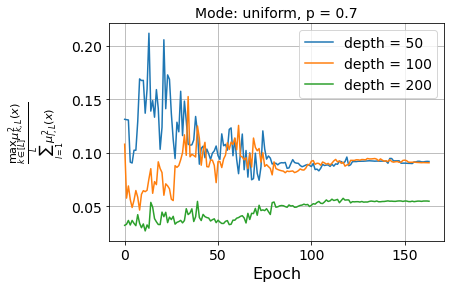
(a) Uniform mode

(b) Linear mode

Figure 6: Empirical verification of assumption 2 of Theorem 2 on Vanilla ResNet with width 256 with average survival probability $\bar{L}/L=0.7$.

(a) Uniform mode

(b) Linear mode

Figure 7: Empirical verification of assumption 2 of Theorem 2 on Vanilla ResNet with width 256 with average survival probability $\bar{L}/L=0.5$.

Figure 8: Empirical verification of Theorem 2 on Vanilla ResNet100 with width 128 with average survival probability $\bar{L}/L=0.7$ and uniform mode. Distribution of the p-values for two normality tests: Shapiro and D’Agostino’s tests

Table 6: Comparison of the modes of selection of the survival probabilities with fixed budget with Stable ResNet56.

$\bar{L}/L$	Uniform	SenseMode	Linear
0.1	24.58 $\pm$ 0.3	2.93 $\pm$ 0.4	$-$
0.2	13.85 $\pm$ 0.3	11.72 $\pm$ 0.3	$-$
0.3	10.23 $\pm$ 0.2	8.59 $\pm$ 0.4	$-$
0.4	8.49 $\pm$ 0.2	8.23 $\pm$ 0.3	$-$
0.5	8.38 $\pm 0.2$	8.25 $\pm$ 0.3	12.01 $\pm$ 0.3
0.6	7.34 $\pm 0.3$	8.17 $\pm$ 0.2	9.26 $\pm$ 0.2
0.7	8.03 $\pm$ 0.1	8.20 $\pm$ 0.1	8.30 $\pm$ 0.1
0.8	6.48 $\pm$ 0.1	7.55 $\pm$ 0.1	6.89 $\pm$ 0.2
0.9	7.16 $\pm$ 0.1	7.81 $\pm$ 0.1	6.62 $\pm$ 0.1
1	$7.10\pm 0.1$

(a) CIFAR10 with ResNet56

$\bar{L}/L$	Uniform	SenseMode	Linear
0.1	61.98 $\pm$ 0.3	60,27 $\pm$ 0.2	$-$
0.2	47.24 $\pm$ 0.2	45.74 $\pm$ 0.3	$-$
0.3	39.38 $\pm$ 0.2	37,11 $\pm$ 0.2	$-$
0.4	35,54 $\pm$ 0.2	33,71 $\pm$ 0.4	$-$
0.5	32.32 $\pm$ 0.1	31 $\pm$ 0.3	40,71 $\pm$ 0.2
0.6	29.57 $\pm$ 0.1	30.19 $\pm$ 0.3	34.13 $\pm$ 0.1
0.7	28.49 $\pm$ 0.4	29.69 $\pm$ 0.1	30.14 $\pm$ 0.1
0.8	27.23 $\pm$ 0.2	29.31 $\pm$ 0.2	28.34 $\pm$ 0.2
0.9	27.01 $\pm$ 0.1	29,45 $\pm$ 0.2	27,35 $\pm$ 0.2
1	28.93 $\pm$ 0.5

(b) Cifar100 with ResNet56

References

- Huang et al. [2016] Gao Huang, Yu Sun, Zhuang Liu, Daniel Sedra, and Kilian Q Weinberger. Deep networks with stochastic depth. In European conference on computer vision, pages 646–661. Springer, 2016.
- Hinton et al. [2012] Geoffrey E Hinton, Nitish Srivastava, Alex Krizhevsky, Ilya Sutskever, and Ruslan R Salakhutdinov. Improving neural networks by preventing co-adaptation of feature detectors. arXiv preprint arXiv:1207.0580, 2012.
- Srivastava et al. [2014] Nitish Srivastava, Geoffrey Hinton, Alex Krizhevsky, Ilya Sutskever, and Ruslan Salakhutdinov. Dropout: a simple way to prevent neural networks from overfitting. The journal of machine learning research, 15(1):1929–1958, 2014.
- Wan et al. [2013] Li Wan, Matthew Zeiler, Sixin Zhang, Yann Le Cun, and Rob Fergus. Regularization of neural networks using dropconnect. In International conference on machine learning, pages 1058–1066, 2013.
- Webb [1994] A.R. Webb. Functional approximation by feed-forward networks: a least-squares approach to generalization. IEEE Transactions on Neural Networks, 5(3):363–371, 1994.
- Bishop [1995] Chris M. Bishop. Training with noise is equivalent to tikhonov regularization. Neural Computation, 7(1):108–116, 1995.
- Camuto et al. [2020] A. Camuto, M. Willetts, U. Simsekli, S. J. Roberts, and C. C. Holmes. Explicit regularisation in gaussian noise injections. In Advances in Neural Information Processing Systems, volume 33, pages 16603–16614, 2020.
- Wager et al. [2013] Stefan Wager, Sida Wang, and Percy S Liang. Dropout training as adaptive regularization. In Advances in neural information processing systems, pages 351–359, 2013.
- Mianjy and Arora [2019] Poorya Mianjy and Raman Arora. On dropout and nuclear norm regularization. arXiv preprint arXiv:1905.11887, 2019.
- Helmbold and Long [2015] David P Helmbold and Philip M Long. On the inductive bias of dropout. The Journal of Machine Learning Research, 16(1):3403–3454, 2015.
- Cavazza et al. [2017] Jacopo Cavazza, Pietro Morerio, Benjamin Haeffele, Connor Lane, Vittorio Murino, and René Vidal. Dropout as a low-rank regularizer for matrix factorization. arXiv preprint arXiv:1710.05092, 2017.
- Wei et al. [2020] C. Wei, S. Kakade, and T. Ma. The implicit and explicit regularization effects of dropout. In Proceedings of the 37th International Conference on Machine Learning, Proceedings of Machine Learning Research, pages 10181–10192. PMLR, 2020.
- He et al. [2015] K. He, X. Zhang, S. Ren, and J. Sun. Delving deep into rectifiers: Surpassing human-level performance on imagenet classification. In ICCV, 2015.
- Neal [1995] R.M. Neal. Bayesian Learning for Neural Networks, volume 118. Springer Science & Business Media, 1995.
- Poole et al. [2016] B. Poole, S. Lahiri, M. Raghu, J. Sohl-Dickstein, and S. Ganguli. Exponential expressivity in deep neural networks through transient chaos. In Advances in Neural Information Processing Systems, 2016.
- Schoenholz et al. [2017] S.S. Schoenholz, J. Gilmer, S. Ganguli, and J. Sohl-Dickstein. Deep information propagation. In International Conference on Learning Representations, 2017.
- Yang [2020] G. Yang. Tensor programs iii: Neural matrix laws. arXiv preprint arXiv:2009.10685, 2020.
- Xiao et al. [2018] L. Xiao, Y. Bahri, J. Sohl-Dickstein, S. S. Schoenholz, and P. Pennington. Dynamical isometry and a mean field theory of cnns: How to train 10,000-layer vanilla convolutional neural networks. ICML 2018, 2018.
- Hayou et al. [2019] S. Hayou, A. Doucet, and J. Rousseau. On the impact of the activation function on deep neural networks training. In International Conference on Machine Learning, 2019.
- Hayou et al. [2020] S. Hayou, A. Doucet, and J. Rousseau. Mean-field behaviour of neural tangent kernel for deep neural networks. arXiv preprint arXiv:1905.13654, 2020.
- Hayou et al. [2021a] S. Hayou, E. Clerico, B. He, G. Deligiannidis, A. Doucet, and J. Rousseau. Stable resnet. In Proceedings of The 24th International Conference on Artificial Intelligence and Statistics, pages 1324–1332, 2021a.
- Yang and Schoenholz [2017] G. Yang and S. Schoenholz. Mean field residual networks: On the edge of chaos. In Advances in Neural Information Processing Systems, pages 7103–7114, 2017.
- Hayou et al. [2021b] S. Hayou, J.F. Ton, A. Doucet, and Y.W. Teh. Robust pruning at initialization. In International Conference on Learning Representations, 2021b.
- Jacot et al. [2018] A. Jacot, F. Gabriel, and C. Hongler. Neural tangent kernel: Convergence and generalization in neural networks. In Advances in Neural Information Processing Systems, 2018.
- Arora et al. [2019] S. Arora, S.S. Du, W. Hu, Z. Li, R. Salakhutdinov, and R. Wang. On exact computation with an infinitely wide neural net. In Advances in Neural Information Processing Systems, 2019.
- Keskar et al. [2016] Nitish Shirish Keskar, Dheevatsa Mudigere, Jorge Nocedal, Mikhail Smelyanskiy, and Ping Tak Peter Tang. On large-batch training for deep learning: Generalization gap and sharp minima. arXiv preprint arXiv:1609.04836, 2016.
- Jastrzebski et al. [2018] Stanislaw Jastrzebski, Zachary Kenton, Nicolas Ballas, Asja Fischer, Yoshua Bengio, and Amos Storkey. On the relation between the sharpest directions of dnn loss and the sgd step length. arXiv preprint arXiv:1807.05031, 2018.
- Yao et al. [2018] Zhewei Yao, Amir Gholami, Qi Lei, Kurt Keutzer, and Michael W Mahoney. Hessian-based analysis of large batch training and robustness to adversaries. In Advances in Neural Information Processing Systems, pages 4949–4959, 2018.
- LeCun et al. [2012] Yann A LeCun, Léon Bottou, Genevieve B Orr, and Klaus-Robert Müller. Efficient backprop. In Neural networks: Tricks of the trade, pages 9–48. Springer, 2012.
- Sagun et al. [2017] Levent Sagun, Utku Evci, V Ugur Guney, Yann Dauphin, and Leon Bottou. Empirical analysis of the hessian of over-parametrized neural networks. arXiv preprint arXiv:1706.04454, 2017.
- Krizhevsky et al. [2009] Alex Krizhevsky, Geoffrey Hinton, et al. Learning multiple layers of features from tiny images. 2009.
- He et al. [2016] K. He, X. Zhang, S. Ren, and J. Sun. Deep residual learning for image recognition. In IEEE Conference on Computer Vision and Pattern Recognition, 2016.
- Shapiro and Wilk [1965] Samuel Sanford Shapiro and Martin B Wilk. An analysis of variance test for normality (complete samples). Biometrika, 52(3/4):591–611, 1965.
- Lee et al. [2019] J. Lee, L. Xiao, S. Schoenholz, Y. Bahri, R. Novak, J. Sohl-Dickstein, and J. Pennington. Wide neural networks of any depth evolve as linear models under gradient descent. In Advances in Neural Information Processing Systems. 2019.
- Matthews et al. [2018] A.G. Matthews, J. Hron, M. Rowland, R.E. Turner, and Z. Ghahramani. Gaussian process behaviour in wide deep neural networks. In International Conference on Learning Representations, 2018.
- Lillicrap et al. [2016] T. Lillicrap, D. Cownden, D. Tweed, and C. Akerman. Random synaptic feedback weights support error backpropagation for deep learning. Nature Communications, 7(13276), 2016.
- Neelakantan et al. [2015] A. Neelakantan, L. Vilnis, Quoc V. Le, I. Sutskever, L. Kaiser, K. Kurach, and J. Martens. Adding gradient noise improves learning for very deep networks. arXiv prePrint 1511.06807, 2015.
- D’Agostino [1970] RALPH B. D’Agostino. Transformation to normality of the null distribution of g1. Biometrika, 57(3):679–681, 12 1970. ISSN 0006-3444. doi: 10.1093/biomet/57.3.679. URL https://doi.org/10.1093/biomet/57.3.679.