Approximate Graph Propagation

Abstract.

Efficient computation of node proximity queries such as transition probabilities, Personalized PageRank, and Katz are of fundamental importance in various graph mining and learning tasks. In particular, several recent works leverage fast node proximity computation to improve the scalability of Graph Neural Networks (GNN). However, prior studies on proximity computation and GNN feature propagation are on a case-by-case basis, with each paper focusing on a particular proximity measure.

In this paper, we propose Approximate Graph Propagation (AGP), a unified randomized algorithm that computes various proximity queries and GNN feature propagation, including transition probabilities, Personalized PageRank, heat kernel PageRank, Katz, SGC, GDC, and APPNP. Our algorithm provides a theoretical bounded error guarantee and runs in almost optimal time complexity. We conduct an extensive experimental study to demonstrate AGP’s effectiveness in two concrete applications: local clustering with heat kernel PageRank and node classification with GNNs. Most notably, we present an empirical study on a billion-edge graph Papers100M, the largest publicly available GNN dataset so far. The results show that AGP can significantly improve various existing GNN models’ scalability without sacrificing prediction accuracy.

1. Introduction

Recently, significant research effort has been devoted to compute node proximty queries such as Personalized PageRank (page1999pagerank, ; jung2017bepi, ; Wang2017FORA, ; wei2018topppr, ), heat kernel PageRank (chung2007HKPR, ; yang2019TEA, ) and the Katz score (katz1953Katz, ). Given a node $s$ in an undirected graph $G=(V,E)$ with $|V|=n$ nodes and $|E|=m$ edges, a node proximity query returns an $n$-dimensional vector $\bm{\pi}$ such that $\bm{\pi}(v)$ represents the importance of node $v$ with respect to $s$. For example, a widely used proximity measure is the $L$-th transition probability vector. It captures the $L$-hop neighbors’ information by computing the probability that a $L$-step random walk from a given source node $s$ reaches each node in the graph. The vector form is given by $\bm{\pi}=\left(\mathbf{A}\mathbf{D}^{-1}\right)^{L}\cdot\bm{e}_{s},$ where $\mathbf{A}$ is the adjacency matrix, $\mathbf{D}$ is the diagonal degree matrix with $\mathbf{D}(i,i)=\sum_{j\in V}\mathbf{A}(i,j)$, and $\bm{e}_{s}$ is the one-hot vector with $\bm{e}_{s}(s)=1$ and $\bm{e}_{s}(v)=0,v\neq s$. Node proximity queries find numerous applications in the area of graph mining, such as link prediction in social networks (backstrom2011supervised, ), personalized graph search techniques (jeh2003scaling, ), fraud detection (andersen2008robust, ), and collaborative filtering in recommender networks (gupta2013wtf, ).

In particular, a recent trend in Graph Neural Network (GNN) researches (wu2019SGC, ; klicpera2019GDC, ; Klicpera2018APPNP, ) is to employ node proximity queries to build scalable GNN models. A typical example is SGC (wu2019SGC, ), which simplifies the original Graph Convolutional Network (GCN) (kipf2016GCN, ) with a linear propagation process. More precisely, given a self-looped graph and an $n\times d$ feature matrix $\mathbf{X}$, SGC takes the multiplication of the $L$-th normalized transition probability matrix $\left(\mathbf{D}^{-\frac{1}{2}}\mathbf{A}\mathbf{D}^{-\frac{1}{2}}\right)^{L}$ and the feature matrix $\mathbf{X}$ to form the representation matrix

(1) $$\mathbf{Z}=\left(\mathbf{D}^{-\frac{1}{2}}\cdot\mathbf{A}\cdot\mathbf{D}^{-\frac{1}{2}}\right)^{L}\cdot\bm{X}.$$

If we treat each column of the feature matrix $\mathbf{X}$ as a graph signal vector $\bm{x}$, then the representation matrix $\mathbf{Z}$ can be derived by the augment of $d$ vectors $\bm{\pi}=\left(\mathbf{D}^{-\frac{1}{2}}\mathbf{A}\mathbf{D}^{-\frac{1}{2}}\right)^{L}\cdot\bm{x}$. SGC feeds $\mathbf{Z}$ into a logistic regression or a standard neural network for downstream machine learning tasks such as node classification and link prediction. The $L$-th normalized transition probability matrix $\left(\mathbf{D}^{-\frac{1}{2}}\mathbf{A}\mathbf{D}^{-\frac{1}{2}}\right)^{L}$ can be easily generalized to other node proximity models, such as PPR used in APPNP (Klicpera2018APPNP, ), PPRGo (bojchevski2020scaling, ) and GBP (chen2020GBP, ), and HKPR used in (klicpera2019GDC, ). Compared to the original GCN (kipf2016GCN, ) which uses a full-batch training process and stores the representation of each node in the GPU memory, these proximity-based GNNs decouple prediction and propagation and thus allows mini-batch training to improve the scalability of the models.

Graph Propagation. To model various proximity measures and GNN propagation formulas, we consider the following unified graph propagation equation:

(2) $$\bm{\pi}=\sum_{i=0}^{\infty}w_{i}\cdot\left(\mathbf{D}^{-a}\mathbf{A}\mathbf{D}^{-b}\right)^{i}\cdot\bm{x},$$

where $\mathbf{A}$ denotes the adjacency matrix, $\mathbf{D}$ denotes the diagonal degree matrix, $a$ and $b$ are the Laplacian parameters that take values in $[0,1]$, the sequence of $w_{i}$ for $i=0,1,2,...$ is the weight sequence and $\bm{x}$ is an $n$ dimensional vector. Following the convention of Graph Convolution Networks (kipf2016GCN, ), we refer to $\mathbf{D}^{-a}\mathbf{A}\mathbf{D}^{-b}$ as the propagation matrix, and $\bm{x}$ as the graph signal vector.

A key feature of the graph propagation equation (2) is that we can manipulate parameters $a$, $b$, $w_{i}$ and $\bm{x}$ to obtain different proximity measures. For example, if we set $a=0,b=1,w_{L}=1,w_{i}=0$ for $i=0,\ldots,L-1$, and $\bm{x}=\bm{e}_{s}$, then $\bm{\pi}$ becomes the $L$-th transition probability vector from node $s$. Table 1 summarizes the proximity measures and GNN models that can be expressed by Equation (2).

Approximate Graph Propagation (AGP). In general, it is computational infeasible to compute Equation (2) exactly as the summation goes to infinity. Following (bressan2018sublinear, ; wang2020RBS, ), we will consider an approximate version of the graph propagation equation (2):

Definition 1.0 (Approximate propagation with relative error).

Let $\bm{\pi}$ be the graph propagation vector defined in Equation (2). Given an error threshold $\delta$, an approximate propagation algorithm has to return an estimation vector $\hat{\bm{\pi}}$, such that for any $v\in V$, with $|\bm{\pi}(v)|>\delta$, we have

$$\vspace{-2mm}\left|\bm{\pi}(v)-\hat{\bm{\pi}}(v)\right|\leq\frac{1}{10}\cdot\bm{\pi}(v)$$

with at least a constant probability (e.g. $99\%$).

We note that some previous works (yang2019TEA, ; Wang2017FORA, ) consider the guarantee $\left|\bm{\pi}(v)-\hat{\bm{\pi}}(v)\right|\leq\varepsilon_{r}\cdot\bm{\pi}(v)$ with probability at least $1-p_{f}$, where $\varepsilon_{r}$ is the relative error parameter and $p_{f}$ is the fail probability. However, $\varepsilon_{r}$ and $p_{f}$ are set to be constant in these works. For sake of simplicity and readability, we set $\varepsilon_{r}=1/10$ and $p_{f}=1\%$ and introduce only one error parameter $\delta$, following the setting in (bressan2018sublinear, ; wang2020RBS, ).

Motivations. Existing works on proximity computation and GNN feature propagation are on a case-by-case basis, with each paper focusing on a particular proximity measure. For example, despite the similarity between Personalized PageRank and heat kernel PageRank, the two proximity measures admit two completely different sets of algorithms (see (wei2018topppr, ; Wang2016HubPPR, ; jung2017bepi, ; Shin2015BEAR, ; coskun2016efficient, ) for Personalized PageRank and (yang2019TEA, ; chung2007HKPR, ; chung2018computing, ; kloster2014heat, ) for heat kernel PageRank). Therefore, a natural question is

Is there a universal algorithm that computes the approximate graph propagation with near optimal cost?

Table 1. Typical graph propagation equations.

	Algorithm	$\bm{a}$	$\bm{b}$	$\bm{w_{i}}$	$\bm{\bm{x}}$	Propagation equation
Proximity	$L$-hop transition probability	$0$	$1$	$w_{i}=0(i\neq L),w_{L}=1$	one-hot vector $\bm{e}_{s}$	$\bm{\pi}=\left(\mathbf{A}\mathbf{D}^{-1}\right)^{L}\cdot\bm{e}_{s}$
	PageRank (page1999pagerank, )	$0$	$1$	$\alpha\left(1-\alpha\right)^{i}$	$\frac{1}{n}\cdot\bm{1}$	$\bm{\pi}=\sum_{i=0}^{\infty}\alpha\left(1-\alpha\right)^{i}\cdot\left(\mathbf{A}\mathbf{D}^{-1}\right)^{i}\cdot\frac{\bm{1}}{n}$
	Personalized PageRank (page1999pagerank, )	$0$	$1$	$\alpha\left(1-\alpha\right)^{i}$	teleport probability distribution $x$	$\bm{\pi}=\sum_{i=0}^{\infty}\alpha\left(1-\alpha\right)^{i}\cdot\left(\mathbf{A}\mathbf{D}^{-1}\right)^{i}\cdot\bm{x}$
	single-target PPR (lofgren2013personalized, )	$1$	$0$	$\alpha\left(1-\alpha\right)^{i}$	one-hot vector $\bm{e}_{v}$	$\bm{\pi}=\sum_{i=0}^{\infty}\alpha\left(1-\alpha\right)^{i}\cdot\left(\mathbf{D}^{-1}\mathbf{A}\right)^{i}\cdot\bm{e}_{v}$
	heat kernel PageRank (chung2007HKPR, )	$0$	$1$	$e^{-t}\cdot\frac{t^{i}}{i!}$	one-hot vector $\bm{e}_{s}$	$\bm{\pi}=\sum_{i=0}^{\infty}e^{-t}\cdot\frac{t^{i}}{i!}\cdot\left(\mathbf{A}\mathbf{D}^{-1}\right)^{i}\cdot\bm{e}_{s}$
	Katz (katz1953Katz, )	$0$	$0$	$\beta^{i}$	one-hot vector $\bm{e}_{s}$	$\bm{\pi}=\sum_{i=0}^{\infty}\beta^{i}\mathbf{A}^{i}\cdot\bm{e}_{s}$
GNN	SGC (wu2019SGC, )	$\frac{1}{2}$	$\frac{1}{2}$	$w_{i}=0(i\neq L),w_{L}=1$	the graph signal $\bm{x}$	$\bm{\pi}=\left(\mathbf{D}^{-\frac{1}{2}}\mathbf{A}\mathbf{D}^{-\frac{1}{2}}\right)^{L}\cdot\bm{x}$
	APPNP (Klicpera2018APPNP, )	$\frac{1}{2}$	$\frac{1}{2}$	$\alpha\left(1-\alpha\right)^{i}$	the graph signal $\bm{x}$	$\bm{\pi}=\sum_{i=0}^{L}\alpha\left(1-\alpha\right)^{i}\cdot\left(\mathbf{D}^{-\frac{1}{2}}\mathbf{A}\mathbf{D}^{-\frac{1}{2}}\right)^{i}\cdot\bm{x}$
	GDC (klicpera2019GDC, )	$\frac{1}{2}$	$\frac{1}{2}$	$e^{-t}\cdot\frac{t^{i}}{i!}$	the graph signal $\bm{x}$	$\bm{\pi}=\sum_{i=0}^{L}e^{-t}\cdot\frac{t^{i}}{i!}\cdot\left(\mathbf{D}^{-\frac{1}{2}}\mathbf{A}\mathbf{D}^{-\frac{1}{2}}\right)^{i}\cdot\bm{x}$

Contributions. In this paper, we present AGP, a UNIFIED randomized algorithm that computes Equation (2) with almost optimal computation time and theoretical error guarantee. AGP naturally generalizes to various proximity measures, including transition probabilities, PageRank and Personalized PageRank, heat kernel PageRank, and Katz. We conduct an extensive experimental study to demonstrate the effectiveness of AGP on real-world graphs. We show that AGP outperforms the state-of-the-art methods for local graph clustering with heat kernel PageRank. We also show that AGP can scale various GNN models (including SGC (wu2019SGC, ), APPNP (Klicpera2018APPNP, ), and GDC (klicpera2019GDC, )) up on the billion-edge graph Papers100M, which is the largest publicly available GNN dataset.

2. Preliminary and Related Work

Table 2. Table of notations.

Notation	Description
$G=(V,E)$	undirected graph with vertex and edge sets $V$ and $E$
$n,m$	the numbers of nodes and edges in $G$
$\mathbf{A}$, $\mathbf{D}$	the adjacency matrix and degree matrix of $G$
$N_{u}$, $d_{u}$	the neighbor set and the degree of node $u$
$a,b$	the Laplacian parameters
$\bm{x}$	the graph signal vector in $\mathcal{R}^{n}$, $\left\|\bm{x}\right\|_{2}=1$
$w_{i},Y_{i}$	the $i$-th weight and partial sum $Y_{i}=\sum_{k=i}^{\infty}w_{k}$
$\bm{\pi},\hat{\bm{\pi}}$	the true and estimated propagation vectors in $\mathcal{R}^{n}$
$\bm{r}^{(i)},\hat{\bm{r}}^{(i)}$	the true and estimated $i$-hop residue vectors in $\mathcal{R}^{n}$
$\bm{q}^{(i)},\hat{\bm{q}}^{(i)}$	the true and estimated $i$-hop reserve vectors in $\mathcal{R}^{n}$
$\delta$	the relative error threshold
$\tilde{O}$	the Big-Oh natation ignoring the log factors

In this section, we provide a detailed discussion on how the graph propagation equation (2) models various node proximity measures. Table 2 summarizes the notations used in this paper.

Personalized PageRank (PPR)  (page1999pagerank, ) is developed by Google to rank web pages on the world wide web, with the intuition that ”a page is important if it is referenced by many pages, or important pages”. Given an undirected graph $G=(V,E)$ with $n$ nodes and $m$ edges and a teleporting probability distribution $\bm{x}$ over the $n$ nodes, the PPR vector $\bm{\pi}$ is the solution to the following equation:

(3) $$\vspace{-2mm}\bm{\pi}=\left(1-\alpha\right)\cdot\mathbf{A}\mathbf{D}^{-1}\cdot\bm{\pi}+\alpha\bm{x}.$$

The unique solution to Equation (3) is given by $\bm{\pi}=\sum_{i=0}^{\infty}\alpha\left(1-\alpha\right)^{i}\cdot\left(\mathbf{A}\mathbf{D}^{-1}\right)^{i}\cdot\bm{x}.$

The efficient computation of the PPR vector has been extensively studied for the past decades. A simple algorithm to estimate PPR is the Monte-Carlo sampling (Fogaras2005MC, ), which stimulates adequate random walks from the source node $s$ generated following $\bm{x}$ and uses the percentage of the walks that terminate at node $v$ as the estimation of $\bm{\pi}(v)$. Forward Search (FOCS06_FS, ) conducts deterministic local pushes from the source node $s$ to find nodes with large PPR scores. FORA (Wang2017FORA, ) combines Forward Search with the Monte Carlo method to improve the computation efficiency. TopPPR (wei2018topppr, ) combines Forward Search, Monte Carlo, and Backward Search (lofgren2013personalized, ) to obtain a better error guarantee for top-$k$ PPR estimation. ResAcc (lin2020index, ) refines FORA by accumulating probability masses before each push. However, these methods only work for graph propagation with transition matrix $\mathbf{A}\mathbf{D}^{-1}$. For example, the Monte Carlo method simulates random walks to obtain the estimation, which is not possible with the general propagation matrix $\mathbf{D}^{-a}\mathbf{A}\mathbf{D}^{-b}$.

Another line of research (lofgren2013personalized, ; wang2020RBS, ) studies the single-target PPR, which asks for the PPR value of every node to a given target node $v$ on the graph. The single-target PPR vector for a given node $v$ is defined by the slightly different formula:

(4) $$\bm{\pi}=\left(1-\alpha\right)\cdot\left(\mathbf{D}^{-1}\mathbf{A}\right)\cdot\bm{\pi}+\alpha\bm{e}_{v}.$$

Unlike the single-source PPR vector, the single-target PPR vector $\bm{\pi}$ is not a probability distribution, which means $\sum_{s\in V}\bm{\pi}(s)$ may not equal to $1$. We can also derive the unique solution to Equation (4) by $\bm{\pi}=\sum_{i=0}^{\infty}\alpha\left(1-\alpha\right)^{i}\cdot\left(\mathbf{D}^{-1}\mathbf{A}\right)^{i}\cdot\bm{e}_{v}$.

Heat kernal PageRank is proposed by (chung2007HKPR, ) for high quality community detection. For each node $v\in V$ and the seed node $s$, the heat kernel PageRank (HKPR) $\bm{\pi}(v)$ equals to the probability that a heat kernal random walk starting from node $s$ ends at node $v$. The length $L$ of the random walks follows the Poisson distribution with parameter $t$, i.e. $\Pr[L=i]=\frac{e^{-t}t^{i}}{i!},i=0,\ldots,\infty$. Consequently, the HKPR vector of a given node $s$ is defined as $\bm{\pi}=\sum_{i=0}^{\infty}\frac{e^{-t}t^{i}}{i!}\cdot\left(\mathbf{A}\mathbf{D}^{-1}\right)^{i}\cdot\bm{e}_{s}$, where $\bm{e}_{s}$ is the one-hot vector with $\bm{e}_{s}(s)=1$. This equation fits in the framework of our generalized propagation equation (2) if we set $a=0,b=1,w_{i}=\frac{e^{-t}t^{i}}{i!}$, and $\bm{x}=\bm{e}_{s}$. Similar to PPR, HKPR can be estimated by the Monte Carlo method (chung2018computing, ; yang2019TEA, ) that simulates random walks of Possion distributed length. HK-Relax (kloster2014heat, ) utilizes Forward Search to approximate the HKPR vector. TEA (yang2019TEA, ) combines Forward Search with Monte Carlo for a more accurate estimator.

Katz index (katz1953Katz, ) is another popular proximity measurement to evaluate relative importance of nodes on the graph. Given two node $s$ and $v$, the Katz score between $s$ and $v$ is characterized by the number of reachable paths from $s$ to $v$. Thus, the Katz vector for a given source node $s$ can be expressed as $\bm{\pi}=\sum_{i=0}^{\infty}\mathbf{A}^{i}\cdot\bm{e}_{s},$ where $\mathbf{A}$ is the adjacency matrix and $\bm{e}_{s}$ is the one-hot vector with $\bm{e}_{s}(s)=1$. However, this summation may not converge due to the large spectral span of $\mathbf{A}$. A commonly used fix up is to apply a penalty of $\beta$ to each step of the path, leading to the following definition: $\bm{\pi}=\sum_{i=0}^{\infty}\beta^{i}\cdot\mathbf{A}^{i}\cdot\bm{e}_{s}$. To guarantee convergence, $\beta$ is a constant that set to be smaller than $\frac{1}{\lambda_{1}}$, where $\lambda_{1}$ is the largest eigenvalue of the adjacency matrix $\mathbf{A}$. Similar to PPR, the Katz vector can be computed by iterative multiplying $\bm{e}_{s}$ with $\mathbf{A}$, which runs in $\tilde{O}(m+n)$ time (foster2001faster, ). Katz has been widely used in graph analytic and learning tasks such as link prediction (Liben2003link, ) and graph embedding (ou2016asymmetric, ). However, the $\tilde{O}(m+n)$ computation time limits its scalability on large graphs.

Proximity-based Graph Neural Networks. Consider an undirected graph $G=(V,E)$, where $V$ and $E$ represent the set of vertices and edges. Each node $v$ is associated with a numeric feature vector of dimension $d$. The $n$ feature vectors form an $n\times d$ matrix $\mathbf{X}$. Following the convention of graph neural networks (kipf2016GCN, ; hamilton2017graphSAGE, ), we assume each node in $G$ is also attached with a self-loop. The goal of graph neural network is to obtain an $n\times d^{\prime}$ representation matrix $\mathbf{Z}$, which encodes both the graph structural information and the feature matrix $\mathbf{X}$. Kipf and Welling (kipf2016GCN, ) propose the vanilla Graph Convolutional Network (GCN), of which the $\ell$-th representation $\mathbf{H}^{(\ell)}$ is defined as $\mathbf{H}^{(\ell)}=\sigma\left(\mathbf{{D}^{-\frac{1}{2}}}\mathbf{{A}}\mathbf{{D}^{-\frac{1}{2}}}\mathbf{H}^{(\ell-1)}\mathbf{W}^{(\ell)}\right)$, where $\mathbf{A}$ and $\mathbf{D}$ are the adjacency matrix and the diagonal degree matrix of $G$, $\mathbf{W}^{(\ell)}$ is the learnable weight matrix, and $\sigma(.)$ is a non-linear activation function (a common choice is the Relu function). Let $L$ denote the number of layers in the GCN model. The $0$-th representation $\mathbf{H}^{(0)}$ is set to the feature matrix $\mathbf{X}$, and the final representation matrix $\mathbf{Z}$ is the $L$-th representation $\mathbf{H}^{(L)}$. Intuitively, GCN aggregates the neighbors’ representation vectors from the $(\ell-1)$-th layer to form the representation of the $\ell$-th layer. Such a simple paradigm is proved to be effective in various graph learning tasks (kipf2016GCN, ; hamilton2017graphSAGE, ).

A major drawback of the vanilla GCN is the lack of ability to scale on graphs with millions of nodes. Such limitation is caused by the fact that the vanilla GCN uses a full-batch training process and stores each node’s representation in the GPU memory. To extend GNN to large graphs, a line of research focuses on decoupling prediction and propagation, which removes the non-linear activation function $\sigma(.)$ for better scalability. These methods first apply a proximity matrix to the feature matrix $\mathbf{X}$ to obtain the representation matrix $\mathbf{Z}$, and then feed $\mathbf{Z}$ into logistic regression or standard neural network for predictions. Among them, SGC (wu2019SGC, ) simplifies the vanilla GCN by taking the multiplication of the $L$-th normalized transition probability matrix $\left(\mathbf{D}^{-\frac{1}{2}}\mathbf{A}\mathbf{D}^{-\frac{1}{2}}\right)^{L}$ and the feature matrix $\mathbf{X}$ to form the final presentation $\mathbf{Z}=\left(\mathbf{D}^{-\frac{1}{2}}\mathbf{A}\mathbf{D}^{-\frac{1}{2}}\right)^{L}\cdot\mathbf{X}$. The proximity matrix can be generalized to PPR used in APPNP (Klicpera2018APPNP, ) and HKPR used in GDC (klicpera2019GDC, ). Note that even though the ideas to employ PPR and HKPR models in the feature propagation process are borrowed from APPNP, PPRGo, GBP and GDC, the original papers of APPNP, PPRGo and GDC use extra complex structures to propagate node features. For example, the original APPNP (Klicpera2018APPNP, ) first applies an one-layer neural network to $\mathbf{X}$ before the propagation that $\mathbf{Z}^{(0)}=f_{\theta}(\mathbf{X})$. Then APPNP propagates the feature matrix $\mathbf{X}$ with a truncated Personalized PageRank matrix $\mathbf{Z}^{(L)}=\sum_{i=0}^{L}\alpha\left(1-\alpha\right)^{i}\cdot\left(\mathbf{D}^{-\frac{1}{2}}\mathbf{A}\mathbf{D}^{-\frac{1}{2}}\right)^{i}\cdot f_{\theta}(\mathbf{X})$, where $L$ is the number of layers and $\alpha$ is a constant in $(0,1)$. The original GDC (klicpera2019GDC, ) follows the structure of GCN and employs the heat kernel as the diffusion kernel. For the sake of scalability, we use APPNP to denote the propagation process $\mathbf{Z}=\sum_{i=0}^{L}\alpha\left(1-\alpha\right)^{i}\cdot\left(\mathbf{D}^{-\frac{1}{2}}\mathbf{A}\mathbf{D}^{-\frac{1}{2}}\right)^{i}\cdot\mathbf{X}$, and GDC to denote the propagation process $\mathbf{Z}=\sum_{i=0}^{L}\frac{e^{-t}t^{i}}{i!}\cdot\left(\mathbf{D}^{-\frac{1}{2}}\mathbf{A}\mathbf{D}^{-\frac{1}{2}}\right)^{i}\cdot\mathbf{X}$.

A recent work PPRGo (bojchevski2020scaling, ) improves the scalability of APPNP by employing the Forward Search algorithm (FOCS06_FS, ) to perform the propagation. However, PPRGo only works for APPNP, which, as we shall see in our experiment, may not always achieve the best performance among the three models. Finally, a recent work GBP (chen2020GBP, ) proposes to use deterministic local push and the Monte Carlo method to approximate GNN propagation of the form $\mathbf{Z}=\sum_{i=0}^{L}w_{i}\cdot\left(\mathbf{D}^{-(1-r)}\mathbf{A}\mathbf{D}^{-r}\right)^{i}\cdot\mathbf{X}.$ However, GBP suffers from two drawbacks: 1) it requires $a+b=1$ in Equation (2) to utilize the Monte-Carlo method, and 2) it requires a large memory space to store the random walk matrix generated by the Monte-Carlo method.

3. Basic Propagation

In the next two sections, we present two algorithms to compute the graph propagation equation (2) with the theoretical relative error guarantee in Definition 1.1.

Assumption on graph signal $\bm{x}$. For the sake of simplicity, we assume the graph signal $\bm{x}$ is non-negative. We can deal with the negative entries in $\bm{x}$ by decomposing it into $\bm{x}=\bm{x}^{+}+\bm{x}^{-}$, where $\bm{x}^{+}$ only contains the non-negative entries of $\bm{x}$ and $\bm{x}^{-}$ only contains the negative entries of $\bm{x}$. After we compute $\bm{\pi}^{+}=\sum_{i=0}^{\infty}w_{i}\cdot\left(\mathbf{D}^{-a}\mathbf{A}\mathbf{D}^{-b}\right)^{i}\cdot\bm{x}^{+}$ and $\bm{\pi}^{-}=\sum_{i=0}^{\infty}w_{i}\cdot\left(\mathbf{D}^{-a}\mathbf{A}\mathbf{D}^{-b}\right)^{i}\cdot\bm{x}^{-}$, we can combine $\bm{\pi}^{+}$ and $\bm{\pi}^{-}$ to form $\bm{\pi}=\bm{\pi}^{+}+\bm{\pi}^{-}$. We also assume $\bm{x}$ is normalized, that is $\|\bm{x}\|_{1}=1$.

Assumptions on $w_{i}$. To make the computation of Equation (2) feasible, we first introduce several assumptions on the weight sequence $w_{i}$ for $i\in\{0,1,2,...\}$. We assume $\sum_{i=0}^{\infty}w_{i}=1$. If not, we can perform propagation with $w_{i}^{\prime}=w_{i}/\sum_{i=0}^{\infty}w_{i}$ and rescale the result by $\sum_{i=0}^{\infty}w_{i}$. We also note that to ensure the convergence of Equation 2, the weight sequence $w_{i}$ has to satisfy $\sum_{i=0}^{\infty}w_{i}\lambda_{max}^{i}<\infty$, where $\lambda_{max}$ is the maximum singular value of the propagation matrix $\mathbf{D}^{-a}\mathbf{A}\mathbf{D}^{-b}$. Therefore, we assume that for sufficiently large $i$, $w_{i}\lambda_{max}^{i}$ is upper bounded by a geometric distribution:

Assumption 3.1.

There exists a constant $L_{0}$ and $\lambda<1$, such that for any $i\geq L_{0}$, $w_{i}\cdot\lambda_{max}^{i}\leq\lambda^{i}$.

According to Assumption 3.1, to achieve the relative error in Definition 1.1, we only need to compute the prefix sum $\bm{\pi}=\sum_{i=0}^{L}w_{i}\cdot\left(\mathbf{D}^{-a}\mathbf{A}\mathbf{D}^{-b}\right)^{i}\cdot\bm{x}$, where $L$ equals to $\log_{\lambda}{\delta}=O\left(\log{1\over\delta}\right)$. This property is possessed by all proximity measures discussed in this paper. For example, PageRank and Personalized PageRank set $w_{i}=\alpha\left(1-\alpha\right)^{i}$, where $\alpha$ is a constant. Since the maximum eigenvalue of $\mathbf{A}\mathbf{D}^{-1}$ is $1$, we have $\|\sum_{i=L+1}^{\infty}w_{i}\left(\mathbf{A}\mathbf{D}^{-1}\right)^{i}\cdot\bm{x}\|_{2}\leq\|\sum_{i=L+1}^{\infty}w_{i}\cdot\bm{x}\|_{2}=\sum_{i=L+1}^{\infty}w_{i}\cdot\|\bm{x}\|_{2}\leq\sum_{i=L+1}^{\infty}w_{i}\cdot\|\bm{x}\|_{1}=\sum_{i=L+1}^{\infty}\alpha\cdot\left(1-\alpha\right)^{i}=(1-\alpha)^{L+1}$. In the second inequality, we use the fact that $\|\bm{x}\|_{2}\leq\|\bm{x}\|_{1}$ and the assumption on $\bm{x}$ that $\|\bm{x}\|_{1}=1$. If we set $L=\log_{1-\alpha}\delta=O\left(\log{\frac{1}{\delta}}\right)$, the remaining sum $\|\sum_{i=L+1}^{\infty}w_{i}\cdot\left(\mathbf{A}\mathbf{D}^{-1}\right)^{i}\cdot\bm{x}\|_{2}$ is bounded by $\delta$. By the assumption that $\bm{x}$ is non-negative, we can terminate the propagation at the $L$-th level without obvious error increment. We can prove similar bounds for HKPR, Katz, and transition probability as well. Detailed explanations are deferred to the appendix.

Basic Propagation. As a baseline solution, we can compute the graph propagation equation (2) by iteratively updating the propagation vector $\bm{\pi}$ via matrix-vector multiplications. Similar approaches have been used for computing PageRank, PPR, HKPR and Katz, under the name of Power Iteration or Power Method.

In general, we employ matrix-vector multiplications to compute the summation of the first $L=O\left(\log{1\over\delta}\right)$ hops of Equation (2): $\bm{\pi}=\sum_{i=0}^{L}w_{i}\cdot\left(\mathbf{D}^{-a}\mathbf{A}\mathbf{D}^{-b}\right)^{i}\cdot\bm{x}$. To avoid the $O(nL)$ space of storing vectors $\left(\mathbf{D}^{-a}\mathbf{A}\mathbf{D}^{-b}\right)^{i}\cdot\bm{x},i=0,\ldots,L$, we only use two vectors: the residue and reserve vectors, which are defined as follows.

Definition 3.0.

[residue and reserve] Let $Y_{i}$ denote the partial sum of the weight sequence that $Y_{i}=\sum_{k=i}^{\infty}w_{k},i=0,\ldots,\infty$. Note that $Y_{0}=\sum_{k=0}^{\infty}w_{k}=1$ under the assumption: $\sum_{i=0}^{\infty}w_{i}=1$. At level $i$, the residue vector is defined as $\bm{r}^{(i)}=Y_{i}\cdot\left(\mathbf{D}^{-a}\mathbf{A}\mathbf{D}^{-b}\right)^{i}\cdot\bm{x}$; The reserve vector is defined as $\bm{q}^{(i)}=\frac{w_{i}}{Y_{i}}\cdot\bm{r}^{(i)}=w_{i}\cdot\left(\mathbf{D}^{-a}\mathbf{A}\mathbf{D}^{-b}\right)^{i}\cdot\bm{x}$.

Intuitively, for each node $u\in V$ and level $i\geq 0$, the residue $\bm{r}^{(i)}(u)$ denotes the probability mass to be distributed to node $u$ at level $i$, and the reserve $\bm{q}^{(i)}(u)$ denotes the probability mass that will stay at node $u$ in level $i$ permanently. By Definition 3.1, the graph propagation equation (2) can be expressed as $\bm{\pi}=\sum_{i=0}^{\infty}\bm{q}^{(i)}.$ Furthermore, the residue vector $\bm{r}^{(i)}$ satisfies the following recursive formula:

(5) $$\vspace{-8mm}\bm{r}^{(i+1)}=\frac{Y_{i+1}}{Y_{i}}\cdot\left(\mathbf{D}^{-a}\mathbf{A}\mathbf{D}^{-b}\right)\cdot\bm{r}^{(i)}.$$

We also observe that the reserve vector $\bm{q}^{(i)}$ can be derived from the residue vector $\bm{r}^{(i)}$ by $\bm{q}^{(i)}=\frac{w_{i}}{Y_{i}}\cdot\bm{r}^{(i)}$. Consequently, given a predetermined level number $L$, we can compute the graph propagation equation (2) by iteratively computing the residue vector $\bm{r}^{(i)}$ and reserve vector $\bm{q}^{(i)}$ for $i=0,1,...,L$.

Input: Undirected graph $G=(V,E)$, graph signal vector $\bm{x}$, weights $w_{i}$, number of levels $L$

Output: the estimated propagation vector $\hat{\bm{\pi}}$

1 $\bm{r}^{(0)}\leftarrow\bm{x}$;

2 for $i=0$ to $L-1$ do

3      

4      for each $u\in V$ with nonzero $\bm{r}^{(i)}(u)$ do

5             for each $v\in N_{u}$  do

6                   $\bm{r}^{(i+1)}(v)\leftarrow\bm{r}^{(i+1)}(v)+\left(\frac{Y_{i+1}}{Y_{i}}\right)\cdot\frac{\bm{r}^{(i)}(u)}{d_{v}^{a}\cdot d_{u}^{b}}$;

7            $\bm{q}^{(i)}(u)\leftarrow\bm{q}^{(i)}(u)+\frac{w_{i}}{Y_{i}}\cdot\bm{r}^{(i)}(u)$;

8            

9      $\hat{\bm{\pi}}\leftarrow\hat{\bm{\pi}}+\bm{q}^{(i)}$ and empty $\bm{r}^{(i)},\bm{q}^{(i)}$;

10      

11$\bm{q}^{(L)}=\frac{w_{L}}{Y_{L}}\cdot\bm{r}^{(L)}$ and $\hat{\bm{\pi}}\leftarrow\hat{\bm{\pi}}+\bm{q}^{(L)}$;

12 return $\hat{\bm{\pi}}$;

Algorithm 1 Basic Propagation Algorithm

Algorithm 1 illustrates the pseudo-code of the basic iterative propagation algorithm. We first set $\bm{r}^{(0)}=\bm{x}$ (line 1). For $i$ from $0$ to $L-1$, we compute $\bm{r}^{(i+1)}=\frac{Y_{i+1}}{Y_{i}}\cdot\left(\mathbf{D}^{-a}\mathbf{A}\mathbf{D}^{-b}\right)\cdot\bm{r}^{(i)}$ by pushing the probability mass $\left(\frac{Y_{i+1}}{Y_{i}}\right)\cdot\frac{\bm{r}^{(i)}(u)}{d_{v}^{a}\cdot d_{u}^{b}}$ to each neighbor $v$ of each node $u$ (lines 2-5). Then, we set $\bm{q}^{(i)}=\frac{w_{i}}{Y_{i}}\cdot\bm{r}^{(i)}$ (line 6), and aggregate $\bm{q}^{(i)}$ to $\hat{\bm{\pi}}$ (line 7). We also empty $\bm{r}^{(i)},\bm{q}^{(i)}$ to save memory. After all $L$ levels are processed, we transform the residue of level $L$ to the reserve vector by updating $\hat{\bm{\pi}}$ accordingly (line 8). We return $\hat{\bm{\pi}}$ as an estimator for the graph propagation vector $\bm{\pi}$ (line 9).

Intuitively, each iteration of Algorithm 1 computes the matrix-vector multiplication $\bm{r}^{(i+1)}=\frac{Y_{i+1}}{Y_{i}}\cdot\left(\mathbf{D}^{-a}\mathbf{A}\mathbf{D}^{-b}\right)\cdot\bm{r}^{(i)}$, where $\mathbf{D}^{-a}\mathbf{A}\mathbf{D}^{-b}$ is an $n\times n$ sparse matrix with $m$ non-zero entries. Therefore, the cost of each iteration of Algorithm 1 is $O(m)$. To achieve the relative error guarantee in Definition 1.1, we need to set $L=O\left(\log{\frac{1}{\delta}}\right)$, and thus the total cost becomes $O\left(m\cdot\log{\frac{1}{\delta}}\right)$. Due to the logarithmic dependence on $\delta$, we use Algorithm 1 to compute high-precision proximity vectors as the ground truths in our experiments. However, the linear dependence on the number of edges $m$ limits the scalability of Algorithm 1 on large graphs. In particular, in the setting of Graph Neural Network, we treat each column of the feature matrix $\mathbf{X}\in\mathcal{R}^{n\times d}$ as the graph signal $\bm{x}$ to do the propagation. Therefore, Algorithm 1 costs $O\left(md\log\frac{1}{\delta}\right)$ to compute the representation matrix $\mathbf{Z}$. Such high complexity limits the scalability of the existing GNN models.

4. Randomized PROPAGATION

A failed attempt: pruned propagation. The $O\left(m\log\frac{1}{\delta}\right)$ running time is undesirable in many applications. To improve the scalability of the basic propagation algorithm, a simple idea is to prune the nodes with small residues in each iteration. This approach has been widely adopted in local clustering methods such as Nibble and PageRank-Nibble (FOCS06_FS, ). In general, there are two schemes to prune the nodes: 1) we can ignore a node $u$ if its residue $\hat{\bm{r}}^{(i)}(u)$ is smaller than some threshold $\varepsilon$ in line 3 of Algorithm 1, or 2) in line 4 of Algorithm 1, we can somehow ignore an edge $(u,v)$ if $\left(\frac{Y_{i+1}}{Y_{i}}\right)\cdot\frac{\bm{r}^{(i)}(u)}{d_{v}^{a}\cdot d_{u}^{b}}$, the residue to be propagated from $u$ to $v$, is smaller than some threshold $\varepsilon^{\prime}$. Intuitively, both pruning schemes can reduce the number of operations in each iteration.

However, as it turns out, the two approaches suffer from either unbounded error or large time cost. More specifically, consider the toy graph shown in Figure 1, on which the goal is to estimate $\bm{\pi}=\left(\mathbf{A}\mathbf{D}^{-1}\right)^{2}\cdot\bm{e}_{s}$, the transition probability vector of a 2-step random walk from node $s$. It is easy to see that $\bm{\pi}(v)=1/2,\bm{\pi}(s)=1/2$, and $\bm{\pi}(u_{i})=0,i=1,\ldots,n$. By setting the relative error threshold $\delta$ as a constant (e.g. $\delta=1/4$), the approximate propagation algorithm has to return a constant approximation of $\bm{\pi}(v)$.

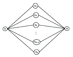
Figure 1. A bad-case graph for pruned propagation.

We consider the first iteration, which pushes the residue $\bm{r}^{(0)}(s)=1$ to $u_{1},\ldots,u_{n}$. If we adopt the first pruning scheme that performs push on $s$ when the residue is large, then we will have to visit all $n$ neighbors of $s$, leading to an intolerable time cost of $O(n)$. On the other hand, we observe that the residue transforms from $s$ to any neighbor $u_{i}$ is $\frac{\bm{r}^{(0)}(s)}{d_{s}}=\frac{1}{n}$. Therefore, if we adopt the second pruning scheme which only performs pushes on edges with large residues to be transformed to, we will simply ignore all pushes from $s$ to $u_{1},\ldots,u_{n}$ and make the incorrect estimation that $\hat{\bm{\pi}}(v)=0$. The problem becomes worse when we are dealing with the general graph propagation equation (2), where the Laplacian parameters $a$ and $b$ in the transition matrix $\mathbf{D}^{-a}\mathbf{A}\mathbf{D}^{-b}$ may take arbitrary values. For example, to the best of our knowledge, no sub-linear approximate algorithm exists for Katz index where $a=b=0$.

Randomized propagation. We solve the above dilemma by presenting a simple randomized propagation algorithm that achieves both theoretical approximation guarantee and near-optimal running time complexity. Algorithm 2 illustrates the pseudo-code of the Randomized Propagation Algorithm, which only differs from Algorithm 1 by a few lines. Similar to Algorithm 1, Algorithm 2 takes in an undirected graph $G=(V,E)$, a graph signal vector $\bm{x}$, a level number $L$ and a weight sequence $w_{i}$ for $i\in[0,L]$. In addition, Algorithm 2 takes in an extra parameter $\varepsilon$, which specifies the relative error guarantee. As we shall see in the analysis, $\varepsilon$ is roughly of the same order as the relative error threshold $\delta$ in Definition 1.1. Similar to Algorithm 1, we start with $\bm{\hat{r}}^{(0)}=\bm{x}$ and iteratively perform propagation through level 0 to level $L$. Here we use $\bm{\hat{r}}^{(i)}$ and $\bm{\hat{q}}^{(i)}$ to denote the estimated residue and reserve vectors at level $i$, respectively. The key difference is that, on a node $u$ with non-zero residue $\hat{\bm{r}}^{(i)}(u)$, instead of pushing the residue to the whole neighbor set $N_{u}$, we only perform pushes to the neighbor $v$ with small degree $d_{v}$. More specifically, for each neighbor $v\in N(u)$ with degree $d_{v}\leq\left(\frac{1}{\varepsilon}\cdot\frac{Y_{i+1}}{Y_{i}}\cdot\frac{\hat{\bm{r}}^{(i)}(u)}{d_{u}^{b}}\right)^{1/a}$, we increase $v$’s residue by $\frac{Y_{i+1}}{Y_{i}}\cdot\frac{\hat{\bm{{r}}}^{(i)}(u)}{d_{v}^{a}\cdot d_{u}^{b}}$, which is the same value as in Algorithm 1. We also note that the condition $d_{v}\leq\left(\frac{1}{\varepsilon}\cdot\frac{Y_{i+1}}{Y_{i}}\cdot\frac{\hat{\bm{r}}^{(i)}(u)}{d_{u}^{b}}\right)^{1/a}$ is equivalent to $\frac{Y_{i+1}}{Y_{i}}\cdot\frac{\hat{\bm{{r}}}^{(i)}(u)}{d_{v}^{a}\cdot d_{u}^{b}}>\varepsilon$, which means we push the residue from $u$ to $v$ only if it is larger than $\varepsilon$. For the remaining nodes in $N_{u}$, we sample each neighbor $v\in N_{u}$ with probability $p_{v}=\frac{1}{\varepsilon}\cdot\frac{Y_{i+1}}{Y_{i}}\cdot\frac{\hat{\bm{r}}^{(i)}(u)}{d_{v}^{a}\cdot d_{u}^{b}}$. Once a node $v$ is sampled, we increase the residue of $v$ by $\varepsilon$. The choice of $p_{v}$ is to ensure that $p_{v}\cdot\varepsilon$, the expected residue increment of $v$, equals to $\frac{Y_{i+1}}{Y_{i}}\cdot\frac{\hat{\bm{r}}^{(i)}(u)}{d_{v}^{a}\cdot d_{u}^{b}}$, the true residue increment if we perform the actual propagation from $u$ to $v$ in Algorithm 1.

Input: undirected graph $G=(V,E)$, graph signal vector $\bm{x}$ with $\|\bm{x}\|_{1}\leq 1$, weighted sequence $w_{i}(i=0,1,...,L)$, error parameter $\varepsilon$, number of levels $L$

Output: the estimated propagation vector $\hat{\bm{\pi}}$

1 $\bm{\hat{r}}^{(0)}\leftarrow\bm{x}$;

2 for $i=0$ to $L-1$ do

3       for each $u\in V$ with non-zero residue $\hat{\bm{r}}^{(i)}(u)$ do

4             for each $v\in N_{u}$ and $d_{v}\leq\left(\frac{1}{\varepsilon}\cdot\frac{Y_{i+1}}{Y_{i}}\cdot\frac{\hat{\bm{r}}^{(i)}(u)}{d_{u}^{b}}\right)^{\frac{1}{a}}$ do

5                   $\bm{\hat{r}}^{(i+1)}(v)\leftarrow\bm{\hat{r}}^{(i+1)}(v)+\frac{Y_{i+1}}{Y_{i}}\cdot\frac{\hat{\bm{r}}^{(i)}(u)}{d_{v}^{a}\cdot d_{u}^{b}}$;

6            Subset Sampling: Sample each remaining neighbor $v\in N_{u}$ with probability $p_{v}=\frac{1}{\varepsilon}\cdot\frac{Y_{i+1}}{Y_{i}}\cdot\frac{\hat{\bm{r}}^{(i)}(u)}{d_{u}^{b}}\cdot\frac{1}{d_{v}^{a}}$;

7             for each sampled neighbor $v\in N(u)$ do

8                   $\bm{\hat{r}}^{(i+1)}(v)\leftarrow\bm{\hat{r}}^{(i+1)}(v)+\varepsilon$;

9                  

10            $\bm{\hat{q}}^{(i)}(u)\leftarrow\bm{\hat{q}}^{(i)}(u)+\frac{w_{i}}{Y_{i}}\cdot\hat{\bm{r}}^{(i)}(u)$;

11            

12      $\hat{\bm{\pi}}\leftarrow\hat{\bm{\pi}}+\hat{\bm{q}}^{(i)}$ and empty $\hat{\bm{r}}^{(i)},\hat{\bm{q}}^{(i)}$;

13      

14$\bm{q}^{(L)}=\frac{w_{L}}{Y_{L}}\cdot\bm{r}^{(L)}$ and $\hat{\bm{\pi}}\leftarrow\hat{\bm{\pi}}+\bm{q}^{(L)}$;

15 return $\bm{\hat{\pi}}$;

Algorithm 2 Randomized Propagation Algorithm

There are two key operations in Algorithm 2. First of all, we need to access the neighbors with small degrees. Secondly, we need to sample each (remaining) neighbor $v\in N_{u}$ according to some probability $p_{v}$. Both operations can be supported by scanning over the neighbor set $N_{u}$. However, the cost of the scan is asymptotically the same as performing a full propagation on $u$ (lines 4-5 in Algorithm 1), which means Algorithm 2 will lose the benefit of randomization and essentially become the same as Algorithm 1.

Pre-sorting adjacency list by degrees. To access the neighbors with small degrees, we can pre-sort each adjacency list $N_{u}$ according to the degrees. More precisely, we assume that $N_{u}=\{v_{1},\ldots,v_{d_{u}}\}$ is stored in a way that $d_{v_{1}}\leq\ldots\leq d_{v_{d_{u}}}$. Consequently, we can implement lines 4-5 in Algorithm 2 by sequentially scanning through $N_{u}=\{v_{1},\ldots,v_{d_{u}}\}$ and stopping at the first $v_{j}$ such that $d_{v_{j}}>\left(\frac{1}{\varepsilon}\cdot\frac{Y_{i+1}}{Y_{i}}\cdot\frac{\hat{\bm{r}}^{(i)}(u)}{d_{u}^{b}}\right)^{1/a}$. With this implementation, we only need to access the neighbors with degrees that exceed the threshold. We also note that we can pre-sort the adjacency lists when reading the graph into the memory, without increasing the asymptotic cost. In particular, we construct a tuple $(u,v,d_{v})$ for each edge $(u,v)$ and use counting sort to sort $(u,v,d_{v})$ tuples in the ascending order of $d_{v}$. Then we scan the tuple list. For each $(u,v,d_{v})$, we append $v$ to the end of $u$’s adjacency list $N_{u}$. Since each $d_{v}$ is bounded by $n$, and there are $m$ tuples, the cost of counting sort is bounded by $O(m+n)$, which is asymptotically the same as reading the graphs.

Subset Sampling. The second problem, however, requires a more delicate solution. Recall that the goal is to sample each neighbor $v_{j}\in N_{u}=\{v_{1},\ldots,v_{d_{u}}\}$ according to the probability $p_{v_{j}}=\frac{Y_{i+1}}{\varepsilon\cdot Y_{i}}\cdot\frac{\hat{\bm{r}}^{(i)}(u)}{d_{v_{j}}^{a}\cdot d_{u}^{b}}$ without touching all the neighbors in $N_{u}$. This problem is known as the Subset Sampling problem and has been solved optimally in (bringmann2012efficient, ). For ease of implementation, we employ a simplified solution: for each node $u\in V$, we partition $u$’s adjacency list $N_{u}=\{v_{1},\ldots,v_{d_{u}}\}$ into $O(\log n)$ groups, such that the $k$-th group $G_{k}$ consists of the neighbors $v_{j}\in N_{u}$ with degrees $d_{v_{j}}\in[2^{k},2^{k+1})$. Note that this can be done by simply sorting $N_{u}$ according to the degrees. Inside the $k$-th group $G_{k}$, the sampling probability $p_{v_{j}}=\frac{Y_{i+1}}{\varepsilon\cdot Y_{i}}\cdot\frac{\hat{\bm{r}}^{(i)}(u)}{d_{v_{j}}^{a}\cdot d_{u}^{b}}$ differs by a factor of at most $2^{a}\leq 2$. Let $p^{*}$ denote the maximum sampling probability in $G_{k}$. We generate a random integer $\ell$ according to the Binomial distribution $B(|G_{k}|,p^{*})$, and randomly selected $\ell$ neighbors from $G_{k}$. For each selected neighbor $v_{j}$, we reject it with probability $1-p_{v_{j}}/p^{*}$. Hence, the sampling complexity for $G_{k}$ can be bounded by $O\left(\sum_{j\in G_{k}}p_{v_{j}}+1\right)$, where $O(1)$ corresponds to the cost to generate the binomial random integer $\ell$ and $O\left(\sum_{j\in G_{k}}p_{j}\right)=O\left(\sum_{j\in G_{k}}p^{*}\right)$ denotes the cost to select $\ell$ neighbors from $G_{k}$. Consequently, the total sampling complexity becomes $O\left(\sum_{k=1}^{\log n}\left(\sum_{j\in G_{k}}p_{j}+1\right)\right)=O\left(\sum_{j=0}^{d_{u}}p_{j}+\log n\right)$. Note that for each subset sampling operation, we need to return $O\left(\sum_{j=0}^{d_{u}}p_{j}\right)$ neighbors in expectation, so this complexity is optimal up to the $\log n$ additive term.

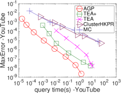
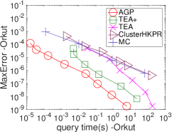
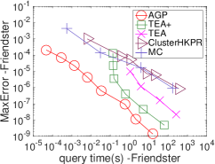
Figure 2. Tradeoffs between MaxError and query time in local clustering.

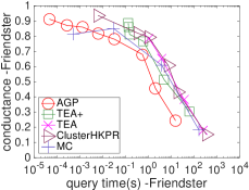
Figure 3. Tradeoffs between conductance and query time in local clustering.

Analysis. We now present a series of lemmas that characterize the error guarantee and the running time of Algorithm 2. For readability, we only give some intuitions for each lemma and defer the detailed proofs to the technical report (TechnicalReport, ). We first present a lemma to show Algorithm 2 can return unbiased estimators for the residue and reserve vectors at each level.

Lemma 4.1.

For each node $v\in V$, Algorithm 2 computes estimators $\bm{\hat{r}}^{(\ell)}(v)$ and $\bm{\hat{q}}^{(\ell)}(v)$ such that $\mathrm{E}\left[\bm{\hat{q}}^{(\ell)}(v)\right]=\bm{q}^{(\ell)}(v)$ and $\mathrm{E}\left[\bm{\hat{r}}^{(\ell)}(v)\right]=\bm{r}^{(\ell)}(v)$ holds for $\forall\ell\in\{0,1,2,...,L\}$.

To give some intuitions on the correctness of Lemma 4.1, recall that in lines 4-5 of Algorithm 1, we add $\frac{Y_{i+1}}{Y_{i}}\cdot\frac{\hat{\bm{r}}^{(i)}(u)}{d_{v}^{a}\cdot d_{u}^{b}}$ to each residue $\hat{\bm{r}}^{(i+1)}(v)$ for $\forall v\in N_{u}$. We perform the same operation in Algorithm 2 for each neighbor $v\in N_{u}$ with large degree $d_{v}$. For each remaining neighbor $v\in V$, we add a residue of $\varepsilon$ to $\hat{\bm{r}}^{(i+1)}(v)$ with probability $\frac{1}{\varepsilon}\frac{Y_{i+1}}{Y_{i}}\cdot\frac{\hat{\bm{r}}^{(i)}(u)}{d_{v}^{a}\cdot d_{u}^{b}}$, leading to an expected increment of $\frac{Y_{i+1}}{Y_{i}}\cdot\frac{\hat{\bm{r}}^{(i)}(u)}{d_{v}^{a}\cdot d_{u}^{b}}$. Therefore, Algorithm 2 computes an unbiased estimator for each residue vector $\bm{r}^{(i)}$, and consequently an unbiased estimator for each reserve vector $\bm{q}^{(i)}$.

In the next Lemma, we bound the variance of the approximate graph propagation vector $\hat{\pi}$, which takes a surprisingly simple form.

Lemma 4.2.

For any node $v\in V$, the variance of $\hat{\bm{\pi}}(v)$ obtained by Algorithm 2 satisfies $\mathrm{Var}\left[\hat{\bm{\pi}}(v)\right]\leq\frac{L(L+1)\varepsilon}{2}\cdot\bm{\pi}(v).$

Recall that we can set $L=O(\log 1/\varepsilon)$ to obtain a relative error threshold of $\varepsilon$. Lemma 4.2 essentially states that the variance decreases linearly with the error parameter $\varepsilon$. Such property is desirable for bounding the relative error. In particular, for any node $v$ with $\bm{\pi}(v)>100\cdot\frac{L(L+1)\varepsilon}{2}$, the standard deviation of $\hat{\bm{\pi}}(v)$ is bounded by ${1\over 10}\bm{\pi}(v)$. Therefore, we can set $\varepsilon=\frac{\delta}{50L(L+1)}=\tilde{O}(\delta)$ to obtain the relative error guarantee in Definition 1.1. In particular, we have the following theorem that bounds the expected cost of Algorithm 2 under the relative error guarantee.

Theorem 4.3.

Algorithm 2 achieves an approximate propagation with relative error $\delta$, that is, for any node $v$ with $\bm{\pi}(v)>\delta$, $\left|\bm{\pi}(v)-\hat{\bm{\pi}}(v)\right|\leq\frac{1}{10}\cdot\bm{\pi}(v)$. The expected time cost can be bounded by

$$E[Cost]=O\left(\frac{L^{2}}{\delta}\cdot\sum_{i=1}^{L}\left\|Y_{i}\cdot\left(\mathbf{D}^{-a}\mathbf{A}\mathbf{D}^{-b}\right)^{i}\cdot\bm{x}\right\|_{1}\right).$$

To understand the time complexity in Theorem 4.3, note that by the Pigeonhole principle, $\frac{1}{\delta}\sum_{i=1}^{L}\left\|w_{i}\cdot\left(\mathbf{D}^{-a}\mathbf{A}\mathbf{D}^{-b}\right)^{i}\cdot\bm{x}\right\|_{1}$ is the upper bound of the number of $v\in V$ satisfying $\bm{\pi}(v)\geq\delta$. In the proximity models such as PPR, HKPR and transition probability, this bound is the output size of the propagation, which means Algorithm 2 achieves near optimal time complexity. We defer the detailed explanation to the technical report (TechnicalReport, ).

Furthermore, we can compare the time complexity of Algorithm 2 with other state-of-the-art algorithms in specific applications. For example, in the setting of heat kernel PageRank, the goal is to estimate $\bm{\pi}=\sum_{i=0}^{\infty}e^{-t}\cdot\frac{t^{i}}{i!}\cdot\left(\mathbf{A}\mathbf{D}^{-1}\right)^{i}\cdot\bm{e}_{s}$ for a given node $s$. The state-of-the-art algorithm TEA (yang2019TEA, ) computes an approximate HKPR vector $\hat{\bm{\pi}}$ such that for any $\pi(v)>\delta$, $|\bm{\pi}(v)-\hat{\bm{\pi}}(v)|\leq\frac{1}{10}\cdot\bm{\pi}(v)$ holds for high probability. By the fact that $t$ is the a constant and $\tilde{O}$ is the Big-Oh notation ignoring log factors, the total cost of TEA is bounded by $O\left(t\log n\over\delta\right)=\tilde{O}\left(1\over\delta\right)$. On the other hand, in the setting of HKPR, the time complexity of Algorithm 2 is bounded by

$$O\left(\frac{L^{2}}{\delta}\cdot\sum_{i=1}^{L}\left\|Y_{i}\cdot\left(\cdot\mathbf{A}\mathbf{D}^{-1}\right)^{i}\cdot\bm{e}_{s}\right\|_{1}\right)=\frac{L^{2}}{\delta}\cdot\sum_{i=1}^{L}Y_{i}\leq\frac{L^{3}}{\delta}=\tilde{O}\left(1\over\delta\right).$$

Here we use the facts that $\left\|\left(\mathbf{A}\mathbf{D}^{-1}\right)^{i}\cdot\bm{e}_{s}\right\|_{1}=1$ and $Y_{i}\leq 1$. This implies that under the specific application of estimating HKPR, the time complexity of the more generalized Algorithm 2 is asymptotically the same as the complexity of TEA. Similar bounds also holds for Personalized PageRank and transition probabilities.

Propagation on directed graph. Our generalized propagation structure also can be extended to directed graph by $\pi=\sum_{i=0}^{\infty}w_{i}\cdot\left(\mathbf{D}^{-a}\tilde{\mathbf{A}}\mathbf{D}^{-b}\right)^{i}\cdot\bm{x},$ where $\mathbf{D}$ denotes the diagonal out-degree matrix, and $\tilde{\mathbf{A}}$ represents the adjacency matrix or its transition according to specific applications. For PageRank, single-source PPR, HKPR, Katz we set $\tilde{\mathbf{A}}=\mathbf{A}^{\top}$ with the following recursive equation:

$$\bm{r}^{(i+1)}(v)=\sum_{u\in N_{in}(v)}\left(\frac{Y_{i+1}}{Y_{i}}\right)\cdot\frac{\bm{r}^{(i)}(u)}{d_{out}^{a}(v)\cdot d_{out}^{b}(u)}.$$

where $N_{in}(v)$ denotes the in-neighbor set of $v$ and $d_{out}(u)$ denotes the out-degree of $u$. For single-target PPR, we set $\tilde{\mathbf{A}}=\mathbf{A}$.

5. Experiments

Table 3. Datasets for local clustering.

Data Set	Type	$\bm{n}$	$\bm{m}$
YouTube	undirected	1,138,499	5,980,886
Orkut-Links	undirected	3,072,441	234,369,798
Twitter	directed	41,652,230	1,468,364,884
Friendster	undirected	68,349,466	3,623,698,684

This section experimentally evaluates AGP’s performance in two concrete applications: local clustering with heat kernel PageRank and node classification with GNN. Specifically, Section 5.1 presents the experimental results of AGP in local clustering. Section 5.2 evaluates the effectiveness of AGP on existing GNN models.

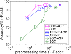
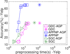
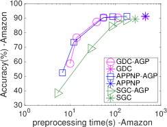
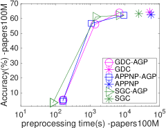
Figure 4. Tradeoffs between Accuracy(%) and preprocessing time in node classification (Best viewed in color).

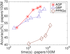
Figure 5. Comparison with GBP, PPRGo and ClusterGCN.

5.1. Local clustering with HKPR

In this subsection, we conduct experiments to evaluate the performance of AGP in local clustering problem. We select HKPR among various node proximity measures as it achieves the state-of-the-art result for local clustering (chung2018computing, ; kloster2014heat, ; yang2019TEA, ).

Datasets and Environment. We use three undirected graphs: YouTube, Orkut, and Friendster in our experiments, as most of the local clustering methods can only support undirected graphs. We also use a large directed graph Twitter to demonstrate AGP’s effectiveness on directed graphs. The four datasets can be obtained from (snapnets, ; LWA, ). We summarize the detailed information of the four datasets in Table 3.

Methods. We compare AGP with four local clustering methods: TEA (yang2019TEA, ) and its optimized version TEA+, ClusterHKPR (chung2018computing, ), and the Monte-Carlo method (MC). We use the results derived by the Basic Propagation Algorithm 1 with $L=50$ as the ground truths for evaluating the trade-off curves of the approximate algorithms. Detailed descriptions on parameter settings are deferred to the appendix due to the space limits.

Metrics. We use MaxError as our metric to measure the approximation quality of each method. MaxError is defined as $MaxError=\max_{v\in V}\left|\frac{\bm{\pi}(v)}{d_{v}}-\frac{\bm{\bm{\hat{\pi}}}(v)}{d_{v}}\right|$, which measures the maximum error between the true normalized HKPR and the estimated value. We refer to $\frac{\bm{\pi}(v)}{d_{v}}$ as the normalized HKPR value from $s$ to $v$. On directed graph, $d_{v}$ is substituted by the out-degree $d_{out}(v)$.

We also consider the quality of the cluster algorithms, which is measured by the conductance. Given a subset $S\subseteq V$, the conductance is defined as $\Phi(S)=\frac{|cut(S)|}{\min\{vol(S),2m-vol(S)\}}$, where $vol(S)=\sum_{v\in S}d(v)$, and $cut(S)=\{(u,v)\in E\mid u\in S,v\in V-S\}$. We perform a sweeping algorithm (Teng2004Nibble, ; FOCS06_FS, ; chung2007HKPR, ; chung2018computing, ; yang2019TEA, ) to find a subset $S$ with small conductance. More precisely, after deriving the (approximate) HKPR vector from a source node $s$, we sort the nodes $\{v_{1},\ldots,v_{n}\}$ in descending order of the normalized HKPR values that $\frac{\bm{\pi}(v_{1})}{d_{v_{1}}}\geq\frac{\bm{\pi}(v_{2})}{d_{v_{2}}}\geq\ldots\geq\frac{\bm{\pi}(v_{n})}{d_{v_{n}}}$. Then, we sweep through $\{v_{1},\ldots,v_{n}\}$ and find the node set with the minimum conductance among partial sets $S_{i}=\{v_{1},\ldots,v_{i}\},i=1,\ldots,n-1$.

Experimental Results. Figure 2 plots the trade-off curve between the MaxError and query time. The time of reading graph is not counted in the query time. We observe that AGP achieves the lowest curve among the five algorithms on all four datasets, which means AGP incurs the least error under the same query time. As a generalized algorithm for the graph propagation problem, these results suggest that AGP outperforms the state-of-the-art HKPR algorithms in terms of the approximation quality.

To evaluate the quality of the clusters found by each method, Figure 3 shows the trade-off curve between conductance and the query time on two large undirected graphs Orkut and Friendster. We observe that AGP can achieve the lowest conductance-query time curve among the five approximate methods on both of the two datasets, which concurs with the fact that AGP provides estimators that are closest to the actual normalized HKPR.

5.2. Node classification with GNN

In this section, we evaluate AGP’s ability to scale existing Graph Neural Network models on large graphs.

Datasets. We use four publicly available graph datasets with different size: a socal network Reddit (hamilton2017graphSAGE, ), a customer interaction network Yelp (zeng2019graphsaint, ), a co-purchasing network Amazon (chiang2019clusterGCN, ) and a large citation network Papers100M (hu2020ogb, ). Table 4 summarizes the statistics of the datasets, where $d$ is the dimension of the node feature, and the label rate is the percentage of labeled nodes in the graph. A detailed discussion on datasets is deferred to the appendix.

Table 4. Datasets for node classification.

Data Set	$\bm{n}$	$\bm{m}$	$\bm{d}$	Classes	Label $\%$
Reddit	232,965	114,615,892	602	41	0.0035
Yelp	716,847	6,977,410	300	100	0.7500
Amazon	2,449,029	61,859,140	100	47	0.7000
Papers100M	111,059,956	1,615,685,872	128	172	0.0109

GNN models. We first consider three proximity-based GNN models: APPNP (Klicpera2018APPNP, ),SGC (wu2019SGC, ), and GDC (klicpera2019GDC, ). We augment the three models with the AGP Algorithm 2 to obtain three variants: APPNP-AGP, SGC-AGP and GDC-AGP. Besides, we also compare AGP with three scalable methods: PPRGo (bojchevski2020scaling, ), GBP (chen2020GBP, ), and ClusterGCN (chiang2019clusterGCN, ).

Experimental results. For GDC, APPNP and SGC, we divide the computation time into two parts: the preprocessing time for computing $\mathbf{Z}$ and the training time for performing mini-batch. Accrording to (chen2020GBP, ), the preprocessing time is the main bottleneck for achieving scalability. Hence, in Figure 4, we show the trade-off between the preprocessing time and the classification accuracy for SGC, APPNP, GDC and the corresponding AGP models. For each dataset, the three snowflakes represent the exact methods SGC, APPNP, and GDC, which can be distinguished by colors. We observe that compared to the exact models, the approximate models generally achieve a $10\times$ speedup in preprocessing time without sacrificing the classification accuracy. For example, on the billion-edge graph Papers100M, SGC-AGP achieves an accuracy of $62\%$ in less than $2,000$ seconds, while the exact model SGC needs over $20,000$ seconds to finish.

Furthermore, we compare AGP against three recent works, PPRGo, GBP, ClusterGCN, to demonstrate the efficiency of AGP. Because ClusterGCN cannot be decomposed into propagation phase and traing phase, in Figure 5, we draw the trade-off plot between the computation time (i.e., preprocessing time plus training time) and the classsification accuracy on Amazon and Papers100M. Note that on Papers100M, we omit ClusterGCN because of the out-of-memory problem. We tune $a,b,w_{i}$ in AGP for scalability. The detailed hyper-parameters of each method are summarized in the appendix. We observe AGP outperforms PPRGo and ClusterGCN on both Amazon and Papers100M in terms of accuracy and running time. In particular, given the same running time, AGP achieves a higher accuracy than GBP does on Papers100M. We attribute this quality to the randomization introduced in AGP.

6. Conclusion

In this paper, we propose the concept of approximate graph propagation, which unifies various proximity measures, including transition probabilities, PageRank and Personalized PageRank, heat kernel PageRank, and Katz. We present a randomized graph propagation algorithm that achieves almost optimal computation time with a theoretical error guarantee. We conduct an extensive experimental study to demonstrate the effectiveness of AGP on real-world graphs. We show that AGP outperforms the state-of-the-art algorithms in the specific application of local clustering and node classification with GNNs. For future work, it is interesting to see if the AGP framework can inspire new proximity measures for graph learning and mining tasks.

7. ACKNOWLEDGEMENTS

Zhewei Wei was supported by National Natural Science Foundation of China (NSFC) No. 61972401 and No. 61932001, by the Fundamental Research Funds for the Central Universities and the Research Funds of Renmin University of China under Grant 18XNLG21, and by Alibaba Group through Alibaba Innovative Research Program. Hanzhi Wang was supported by the Outstanding Innovative Talents Cultivation Funded Programs 2020 of Renmin Univertity of China. Sibo Wang was supported by Hong Kong RGC ECS No. 24203419, RGC CRF No. C4158-20G, and NSFC No. U1936205. Ye Yuan was supported by NSFC No. 61932004 and No. 61622202, and by FRFCU No. N181605012. Xiaoyong Du was supported by NSFC No. 62072458. Ji-Rong Wen was supported by NSFC No. 61832017, and by Beijing Outstanding Young Scientist Program NO. BJJWZYJH012019100020098. This work was supported by Public Computing Cloud, Renmin University of China, and by China Unicom Innovation Ecological Cooperation Plan.

Table 5. Hyper-parameters of AGP.

Dataset	Learning	Dropout	Hidden	Batch	$\bm{t}$	$\bm{\alpha}$	$\bm{L}$
	rate		dimension	size
Yelp	0.01	0.1	2048	$3\cdot 10^{4}$	4	0.9	10
Amazon	0.01	0.1	1024	$10^{5}$	4	0.2	10
Reddit	0.0001	0.3	2048	$10^{4}$	3	0.1	10
Papers100M	0.0001	0.3	2048	$10^{4}$	4	0.2	10

Table 6. Hyper-parameters of GBP.

Dataset	Learning	Dropout	Hidden	Batch	$r_{max}$	$r$	$\alpha$
	rate		dimension	size
Amazon	0.01	0.1	1024	$10^{5}$	$10^{-7}$	0.2	0.2
Papers100M	0.0001	0.3	2048	$10^{4}$	$10^{-8}$	0.5	0.2

Table 7. Hyper-parameters of PPRGo.

Dataset	Learning	Dropout	Hidden	Batch	$r_{max}$	$k$	$L$
	rate		dimension	size
Amazon	0.01	0.1	64	$10^{5}$	$5\cdot 10^{-5}$	64	8
Papers100M	0.01	0.1	64	$10^{4}$	$10^{-4}$	32	8

Table 8. Hyper-parameters of ClusterGCN.

Dataset	Learning	Dropout	Hidden	layer	partitions
	rate		dimension
Amazon	0.01	0.2	400	4	15000

Table 9. URLs of baseline codes.

Methods	URL
GDC	https://github.com/klicperajo/gdc
APPNP	https://github.com/rusty1s/pytorch$\_$geometric
SGC	https://github.com/Tiiiger/SGC
PPRGo	https://github.com/TUM-DAML/pprgo$\_$pytorch
GBP	https://github.com/chennnM/GBP
ClusterGCN	https://github.com/benedekrozemberczki/ClusterGCN

Appendix A Experimental Details

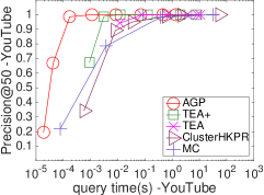
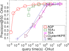
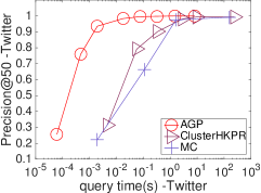
Figure 6. Tradeoffs between Normalized Precision@50 and query time in local clustering.

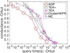
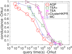
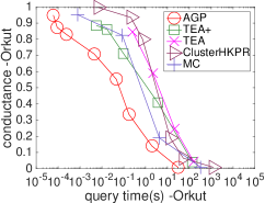
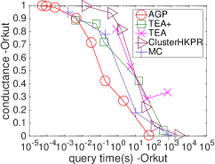
(a) $t=5$	(b) $t=10$	(c) $t=20$	(d) $t=40$

Figure 7. Effect of heat constant t for conductance on Orkut.

A.1. Local clustering with HKPR

Methods and Parameters. For AGP, we set $a=0,b=1,w_{i}=\frac{e^{-t}t^{i}}{i!}$, and $\bm{x}=\bm{e}_{s}$ in Equation (2) to simulate the HKPR equation $\bm{\pi}=\sum_{i=0}^{\infty}\frac{e^{-t}t^{i}}{i!}\cdot\left(\mathbf{A}\mathbf{D}^{-1}\right)^{i}\cdot\bm{e}_{s}$. We employ the randomized propagation algorithm 2 with level number $L=O\left(\log{1/\delta}\right)$ and error parameter $\varepsilon=\frac{2\delta}{L(L+1)}$, where $\delta$ is the relative error threshold in Definition 1.1. We use AGP to denote this method. We vary $\delta$ from $0.1$ to $10^{-8}$ with 0.1 decay step to obtain a trade-off curve between the approximation quality and the query time. We use the results derived by the Basic Propagation Algorithm 1 with $L=50$ as the ground truths for evaluating the trade-off curves of the approximate algorithms.

We compare AGP with four local clustering methods: TEA [41] and its optimized version TEA+, ClusterHKPR [14], and the Monte-Carlo method (MC). TEA [41], as the state-of-the-art clustering method, combines a deterministic push process with the Monte-Carlo random walk. Given a graph $G=(V,E)$, and a seed node $s$, TEA conducts a local search algorithm to explore the graph around $s$ deterministically, and then generates random walks from nodes with residues exceeding a threshold parameter $r_{max}$. One can manipulate $r_{max}$ to balance the two processes. It is shown in [41] that TEA can achieve $O\left(\frac{t\cdot\log{n}}{\delta}\right)$ time complexity, where $t$ is the constant heat kernel parameter. ClusterHKPR [14] is a Monte-Carlo based method that simulates adequate random walks from the given seed node and uses the percentage of random walks terminating at node $v$ as the estimation of $\bm{\pi}(v)$. The length of walks $k$ follows the Poisson distribution $\frac{e^{-t}t^{k}}{k!}$. The number of random walks need to achieve a relative error of $\delta$ in Definition 1.1 is $O\left(\frac{t\cdot\log{n}}{\delta^{3}}\right)$. MC [41] is an optimized version of random walk process that sets identical length for each walk as $L=t\cdot\frac{\log{1/\delta}}{\log{\log{1/\delta}}}$. If a random walk visit node $v$ at the $k$-th step, we add $\frac{e^{-t}t^{k}}{n_{r}\cdot k!}$ to the propagation results $\bm{\bm{\hat{\pi}}}(v)$, where $n_{r}$ denotes the total number of random walks. The number of random walks to achieve a relative error of $\delta$ is also $O\left(\frac{t\cdot\log{n}}{\delta^{3}}\right)$. Similar to AGP, for each method, we vary $\delta$ from $0.1$ to $10^{-8}$ with 0.1 decay step to obtain a trade-off curve between the approximation quality and the query time. Unless specified otherwise, we set the heat kernel parameter $t$ as 5, following [28, 41]. All local clustering experiments are conducted on a machine with an Intel(R) Xeon(R) Gold 6126@2.60GHz CPU and 500GB memory.

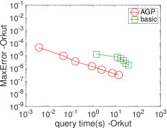
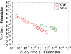
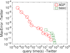
Figure 8. Tradeoffs between MaxError and query time of Katz.

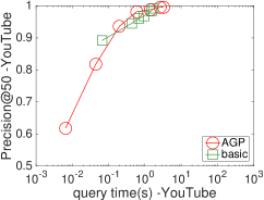
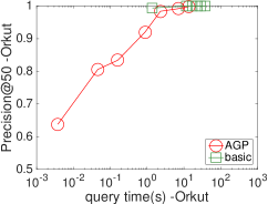
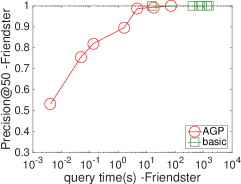
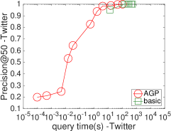
Figure 9. Tradeoffs between Precision@50 and query time of Katz.

A.2. Node classification with GNN

Datasets. Following [42, 43], we perform inductive node classification on Yelp, Amazon and Reddit, and semi-supervised transductive node classification on Papers100M. More specifically, for inductive node classification tasks, we train the model on a graph with labeled nodes and predict nodes’ labels on a testing graph. For semi-supervised transductive node classification tasks, we train the model with a small subset of labeled nodes and predict other nodes’ labels in the same graph. We follow the same training/validation/test-ing split as previous works in GNN [42, 21].

GNN models. We first consider three proximity-based GNN models: APPNP [26],SGC [40], and GDC [27]. We augment the three models with the AGP Algorithm 2 to obtain three variants: APPNP-AGP, SGC-AGP and GDC-AGP. Take SGC-AGP as an example. Recall that SGC uses $\mathbf{Z}=\left(\mathbf{D}^{-\frac{1}{2}}\mathbf{A}\mathbf{D}^{-\frac{1}{2}}\right)^{L}\cdot\mathbf{X}$ to perform feature aggregation, where $\mathbf{X}$ is the $n\times d$ feature matrix. SGC-AGP treats each column of $\mathbf{X}$ as a graph signal $\bm{x}$ and perform randomized propagation algorithm (Algorithm 2) with predetermined error parameter $\delta$ to obtain the the final representation $\mathbf{Z}$. To achieve high parallelism, we perform propagation for multiple columns of $\mathbf{X}$ in parallel. Since APPNP and GDC’s original implementation cannot scale on billion-edge graph Papers100M, we implement APPNP and GDC in the AGP framework. In particular, we set $\varepsilon=0$ in Algorithm 2 to obtain the exact propagation matrix $\mathbf{Z}$, in which case the approximate models APPNP-AGP and GDC-AGP essentially become the exact models APPNP and GDC. We set $L=20$ for GDC-AGP and APPNP-AGP, and $L=10$ for SGC-AGP. Note that SGC suffers from the over-smoothing problem when the number of layers $L$ is large [40]. We vary the parameter $\varepsilon$ to obtain a trade-off curve between the classification accuracy and the computation time.

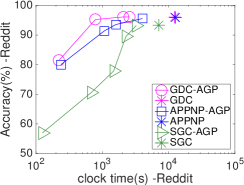
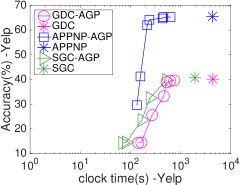
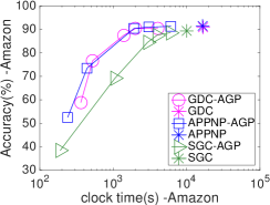
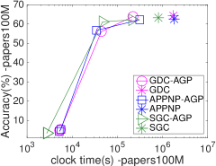
Figure 10. Tradeoffs between Accuracy(%) and clock time in node classification.

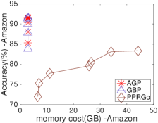
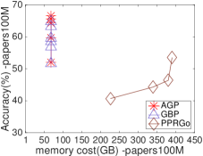
Figure 11. Tradeoffs between Accuracy(%) and memory cost in node classification.

Besides, we also compare AGP with three scalable methods: PPRGo [7], GBP [11], and ClusterGCN [12]. Recall that PPRGo is an improvement work of APPNP. It has three main parameters: the number of non-zero PPR values for each training node $k$, the number of hops $L$, and the residue threshold $r_{max}$. We vary the three parameters $(k,L,r_{max})$ from $(32,2,0.1)$ to $(64,10,10^{-5})$. GBP decouples the feature propagation and prediction to achieve high scalability. In the propagation process, GBP has two parameters: the propagation threshold $r_{max}$ and the level $L$. We vary $r_{max}$ from $10^{-4}$ to $10^{-10}$, and set $L=4$ following [11]. ClusterGCN uses graph sampling method to partition graphs into small parts, and performs the feature propagation on one randomly picked sub-graph in each mini-batch. We vary the partition numbers from $10^{4}$ to $10^{5}$, and the propagation layers from $2$ to $4$.

For each method, we apply a neural network with 4 hidden layers, trained with mini-batch SGD. We employ initial residual connection [20] across the hidden layers to facilitate training. We use the trained model to predict each testing node’s labels and take the mean accuracy after five runs. All the experiments in this section are conducted on a machine with an NVIDIA RTX8000 GPU (48GB memory), Intel Xeon CPU (2.20 GHz) with 40 cores, and 512 GB of RAM.

Detailed setups. In Table 9, we summarize the hyper-parameters of GDC, APPNP, SGC and the corresponding AGP models. Note that the parameter $t$ is for GDC and GDC-AGP, $\alpha$ is for APPNP and APPNP-AGP and $L$ is for SGC and SGC-AGP. We set $a=b=\frac{1}{2}$. In Table 9, Table 9 and Table 9, we summarize the hyper-parameters of GBP, PPRGo and ClusterGNN. For ClusterGCN, we set the number of clusters per batch as $10$ on Amazon, following [12]. For AGP, we set $a=0.8,b=0.2,w_{i}=\alpha(1-\alpha)^{i}$ on Amazon, and $a=b=0.5,w_{i}=e^{-t}\cdot\frac{t^{i}}{i!}$ on Papers100M. The other hyper-parameters of AGP are the same as those in Table 9. In Table 9, we list the available URL of each method.

Appendix B Additional experimental results

B.1. Local clustering with HKPR

Apart from using MaxError to measure the approximation quality, we further explore the trade-off curves between Precision@k and query time. Let $V_{k}$ denote the set of $k$ nodes with highest normalized HKPR values, and $\hat{V}_{k}$ denote the estimated top-$k$ node set returned by an approximate method. Normalized Precision@k is defined as the percentage of nodes in $\hat{V}_{k}$ that coincides with the actual top-$k$ results $V_{k}$. Precision@k can evaluate the accuracy of the relative node order of each method. Similarly, we use the Basic Propagation Algorithm 1 with $L=50$ to obtain the ground truths of the normalized HKPR. Figure 7 plots the trade-off curve between Precision@50 and the query time for each method. We omit TEA and TEA+ on Twitter as they cannot handle directed graphs. We observe that AGP achieves the highest precision among the five approximate algorithms on all four datasets under the same query time.

Besides, we also conduct experiments to present the influence of heat kernel parameter $t$ on the experimental performances. Figure 7 plots the conductance and query time trade-offs on Orkut, with $t$ varying in $\{5,10,20,40\}$. Recall that $t$ is the average length of the heat kernel random walk. Hence, the query time of each method increases as $t$ varying from 5 to 40. We observe that AGP consistently achieves the lowest conductance with the same amount of query time. Furthermore, as $t$ increases from $5$ to $40$, AGP’s query time only increases by $7\times$, while TEA and TEA+ increase by $10\times-100\times$, which demonstrates the scalability of AGP.

B.2. Evaluation of Katz index

Table 10. preprocessing and training time

	APPNP-AGP	GDC-AGP	SGC-AGP	PPRGo
preprocessing time (s)	9253.85	6807.17	1437.95	7639.72
training time (s)	166.19	175.62	120.07	140.67

We also evaluate the performance of AGP to compute the Katz index. Recall that Katz index numerates the paths of all lengths between a pair of nodes, which can be expressed as that $\bm{\pi}=\sum_{i=0}^{\infty}\beta^{i}\cdot\mathbf{A}^{i}\cdot\bm{e}_{s}$. In our experiments, $\beta$ is set as $\frac{0.85}{\lambda_{1}}$ to guarantee convergence, where $\lambda_{1}$ denotes the largest eigenvalue of the adjacent matrix $\bm{A}$. We compare the performance of AGP with the basic propagation algorithm given in Algorithm 1 (denoted as basic in Figure 9,  9). We treat the results computed by the basic propagation algorithm with $L=50$ as the ground truths. Varying $\delta$ from $0.01$ to $10^{8}$, Figure 9 shows the trade-offs between MaxError and query time. Here we define $MaxError=\max_{v\in V}\left|\bm{\pi}(v)-\bm{\bm{\hat{\pi}}}(v)\right|$. We issue 50 query nodes and return the average MaxError of all query nodes same as before. We can observe that AGP costs less time than basic propagation algorithm to achieve the same error. Especially when $\delta$ is large, such as $MaxError=10^{-5}$ on the dataset Orkut, AGP has a $10\times-100\times$ speed up than the basic propagation algorithm. Figure 9 plots the trade-off lines between Precision@50 and query time. The definition of Precision@k is the same as that in Figure 7, which equals the percentage of nodes in the estimated top-k set that coincides with the real top-k nodes. Note that the basic propagation algorithm can always achieve precision 1 even with large MaxError. This is because the propagation results derived by the basic propagation algorithm are always smaller than the ground truths. The biased results may present large error and high precision simultaneously by maintaining the relative order of top-k nodes. While AGP is not a biased method, the precision will increase with the decreasing of MaxError.

B.3. Node classification with GNN

Comparison of clock time. To eliminate the effect of parallelism, we plot the trade-offs between clock time and classification accuracy in Figure 10. We can observe that AGP still achieves a $10\times$ speedup on each dataset, which concurs with the analysis for propagation time. Besides, note that every method presents a nearly $30\times$ speedup after parallelism, which reflects the effectiveness of parallelism.

Comparison of preprocessing time and training time. Table 10 shows the comparison between the training time and preprocessing time on Papers100M. Due to the large batch size ($10,000$), the training process is generally significantly faster than the feature propagation process. Hence, we recognize feature propagation as the bottleneck for scaling GNN models on large graphs, motivating our study on approximate graph propagation.

Comparison of memory cost. Figure 11 shows the memory overhead of AGP, GBP, and PPRGo. Recall that the AGP Algorithm 2 only maintains two $n$ dimension vectors: the residue vector $\bm{r}$ and the reserve vector $\bm{q}$. Consequently, AGP only takes a fixed memory, which can be ignored compared to the graph’s size and the feature matrix. Such property is ideal for scaling GNN models on massive graphs.

Appendix C Proofs

C.1. Chebyshev’s Inequality

Lemma C.1 (Chebyshev’s inequality).

Let $X$ be a random variable, then $\Pr\left[\left|X-\mathrm{E}[X]\right|\geq\varepsilon\right]\leq{\mathrm{Var}[X]\over\varepsilon^{2}}.$

C.2. Further Explanations on Assumption 3.1

Recall that in Section 3, we introduce Assumption 3.1 to guarantee we only need to compute the prefix sum $\bm{\pi}=\sum_{i=0}^{L}w_{i}\cdot\left(\mathbf{D}^{-a}\mathbf{A}\mathbf{D}^{-b}\right)^{i}$ to achieve the relative error in Definition 1.1, where $L=O\left(\log{\frac{1}{\delta}}\right)$. The following theorem offers a formal proof of this property.

Theorem C.2.

According to the assumptions on $w_{i}$ and $\bm{x}$ in Section 3, to achieve the relative error in Definition 1.1, we only need to approximate the prefix sum $\bm{\pi}_{L}=\sum_{i=0}^{L}w_{i}\cdot\left(\mathbf{D}^{-a}\mathbf{A}\mathbf{D}^{-b}\right)^{i}\cdot\bm{x}$, such that for any $v\in V$ with $\bm{\pi}_{L}(v)>\frac{18}{19}\cdot\delta$, we have $\left|\bm{\pi}_{L}(v)-\hat{\bm{\pi}}(v)\right|\leq\frac{1}{20}\bm{\pi}_{L}(v)$ holds with high probability.

Proof.

We first show according to Assumption 3.1 and the assumption $\|\bm{x}\|_{1}=1$, by setting $L=O\left(\log{\frac{1}{\delta}}\right)$, we have:

(6) $$\left\|\sum_{i=L+1}^{\infty}w_{i}\cdot\left(\mathbf{D}^{-a}\mathbf{A}\mathbf{D}^{-b}\right)^{i}\cdot\bm{x}\right\|_{2}\leq\frac{\delta}{19}.$$

Recall that in Assumption 3.1, we assume $w_{i}\cdot\lambda_{max}^{i}$ is upper bounded by $\lambda^{i}$ when $i\geq L_{0}$ and $L_{0}\geq 1$ is a constant. $\lambda_{max}$ denotes the maximum eigenvalue of the transition probability matrix $\mathbf{D}^{-a}\mathbf{A}\mathbf{D}^{-b}$ and $\lambda<1$ is a constant. Thus, for $\forall L\geq L_{0}$, we have:

$$\left\|\sum_{i=L+1}^{\infty}w_{i}\cdot\left(\mathbf{D}^{-a}\mathbf{A}\mathbf{D}^{-b}\right)^{i}\cdot\bm{x}\right\|_{2}\leq\left\|\sum_{i=L+1}^{\infty}w_{i}\cdot\lambda_{max}^{i}\cdot\bm{x}\right\|_{2}\leq\sum_{i=L+1}^{\infty}\lambda^{i}\cdot\left\|\bm{x}\right\|_{2}\leq\sum_{i=L+1}^{\infty}\lambda^{i}.$$

In the last inequality, we use the fact $\|\bm{x}\|_{2}\leq\|\bm{x}\|_{1}=1$. By setting $L=\max\left\{L_{0},O\left(\log_{\lambda}{\frac{(1-\lambda)\cdot\delta}{19}}\right)\right\}=O(\log{\frac{1}{\delta}})$, we can derive:

$$\left\|\sum_{i=L+1}^{\infty}w_{i}\cdot\left(\mathbf{D}^{-a}\mathbf{A}\mathbf{D}^{-b}\right)^{i}\cdot\bm{x}\right\|_{2}\leq\sum_{i=L+1}^{\infty}\lambda^{i}=\frac{\lambda^{L+1}}{1-\lambda}\leq\frac{\delta}{19},$$

which follows the inequality (6).

Then we show that according to the assumption on the non-negativity of $\bm{x}$ and the bound $\left\|\sum_{i=L+1}^{\infty}w_{i}\cdot\left(\mathbf{D}^{-a}\mathbf{A}\mathbf{D}^{-b}\right)^{i}\cdot\bm{x}\right\|_{2}\leq\frac{\delta}{19}$, to achieve the relative error in Definition 1.1, we only need to approximate the prefix sum $\bm{\pi}_{L}=\sum_{i=0}^{L}w_{i}\cdot\left(\mathbf{D}^{-a}\mathbf{A}\mathbf{D}^{-b}\right)^{i}\cdot\bm{x}$. Specifically, we only need to return the vector $\hat{\bm{\pi}}$ as the estimator of $\bm{\pi}_{L}$ such that for any $v\in V$ with $\bm{\pi}_{L}(v)\geq\frac{18}{19}\cdot\delta$, we have

(7) $$\left|\bm{\pi}_{L}(v)-\hat{\bm{\pi}}(v)\right|\leq\frac{1}{20}\bm{\pi}_{L}(v)$$

holds with high probability.

Let $\bm{\pi}_{L}$ denote the prefix sum that $\bm{\pi}_{L}=\sum_{i=0}^{L}w_{i}\cdot\left(\mathbf{D}^{-a}\mathbf{A}\mathbf{D}^{-b}\right)^{i}\cdot\bm{x}$ and $\bm{\bar{\pi}}_{L}$ denote the remaining sum that $\bm{\bar{\pi}}_{L}=\sum_{i=L+1}^{\infty}w_{i}\cdot\left(\mathbf{D}^{-a}\mathbf{A}\mathbf{D}^{-b}\right)^{i}\cdot\bm{x}$. Hence the real propagation vector $\bm{\pi}=\bm{\pi}_{L}+\bm{\bar{\pi}}_{L}=\sum_{i=0}^{\infty}w_{i}\cdot\left(\mathbf{D}^{-a}\mathbf{A}\mathbf{D}^{-b}\right)^{i}\cdot\bm{x}$. For each node $v\in V$ with $\bm{\pi}_{L}(v)>\frac{18}{19}\cdot\delta$, we have:

$$\left|\bm{\pi}(v)-\hat{\bm{\pi}}(v)\right|\leq\left|\bm{\pi}_{L}(v)-\hat{\bm{\pi}}(v)\right|+\bm{\bar{\pi}}(v)$$

$$\leq\frac{1}{20}\bm{\pi}_{L}(v)+\bm{\bar{\pi}}(v)=\frac{1}{20}\bm{\pi}(v)+\frac{19}{20}\bm{\bar{\pi}}(v).$$

In the first inequality, we use the fact that $\bm{\pi}=\bm{\pi}_{L}+\bm{\bar{\pi}}_{L}$ and $\left|\bm{\pi}_{L}(v)-\hat{\bm{\pi}}(v)+\bm{\bar{\pi}}(v)\right|\leq\left|\bm{\pi}_{L}(v)-\hat{\bm{\pi}}(v)\right|+\bm{\bar{\pi}}(v)$. In the second inequality, we apply inequality (7) and the assumption that $\bm{x}$ is non-negative. By the bound that $\bm{\bar{\pi}}(v)\leq\left\|\sum_{i=L+1}^{\infty}w_{i}\cdot\left(\mathbf{D}^{-a}\mathbf{A}\mathbf{D}^{-b}\right)^{i}\cdot\bm{x}\right\|_{2}\leq\frac{1}{19}\delta$, we can derive:

$$\left|\bm{\pi}(v)-\hat{\bm{\pi}}(v)\right|\leq\frac{1}{20}\bm{\pi}(v)+\frac{1}{20}\delta\leq\frac{1}{10}\bm{\pi}(v).$$

In the last inequality, we apply the error threshold in Definition 1.1 that $\bm{\pi}(v)\geq\delta$, and the theorem follows. ∎

Even though we derive Theorem C.2 based on Assumption 3.1, the following lemma shows that without Assumption 3.1, the property of Theorem C.2 is also possessed by all proximity measures discussed in this paper.

Lemma C.3.

In the proximity models of PageRank, PPR, HKPR, transition probability and Katz, Theorem C.2 holds without Assumption 3.1.

Proof.

We first show in the proximity models of PageRank, PPR, HKPR, transition probability and Katz, by setting $L=O\left(\log{\frac{1}{\delta}}\right)$, we can bound

(8) $$\left\|\sum_{i=L+1}^{\infty}w_{i}\cdot\left(\mathbf{D}^{-a}\mathbf{A}\mathbf{D}^{-b}\right)^{i}\cdot\bm{x}\right\|_{2}\leq\frac{\delta}{19},$$

only based on the assumptions that $\bm{x}$ is non-negative and $\|\bm{x}\|_{1}=1$, without Assumption 3.1.

In the proximity model of PageRank, PPR, HKPR and transition probability, we set $a=b=1$ and the transition probability matrix is $\mathbf{D}^{-a}\mathbf{A}\mathbf{D}^{-b}=\mathbf{A}\mathbf{D}^{-1}$. Thus, the left side of inequality (8) becomes $\left\|\sum_{i=L+1}^{\infty}w_{i}\cdot\left(\mathbf{A}\mathbf{D}^{-1}\right)^{i}\cdot\bm{x}\right\|_{2}=\sum_{i=L+1}^{\infty}w_{i}\cdot\left\|\left(\mathbf{A}\mathbf{D}^{-1}\right)^{i}\cdot\bm{x}\right\|_{2}$, where we apply the assumption on the non-negativity of $\bm{x}$. Because the maximum eigenvalue of the matrix $\mathbf{A}\mathbf{D}^{-1}$ is $1$, we have $\left\|\left(\mathbf{A}\mathbf{D}^{-1}\right)^{i}\cdot\bm{x}\right\|_{2}\leq\|\bm{x}\|_{2}$, following:

$$\sum_{i=L+1}^{\infty}w_{i}\cdot\left\|\left(\mathbf{A}\mathbf{D}^{-1}\right)^{i}\cdot\bm{x}\right\|_{2}\leq\sum_{i=L+1}^{\infty}w_{i}\cdot\|\bm{x}\|_{2}\leq\sum_{i=L+1}^{\infty}w_{i}\cdot\|\bm{x}\|_{1}=\sum_{i=L+1}^{\infty}w_{i}.$$

In the last equality, we apply the assumption that $\|\bm{x}\|_{1}=1$. Hence, for PageRank, PPR, HKPR and transition probability, we only need to show $\sum_{i=L+1}^{\infty}w_{i}\leq\frac{\delta}{19}$ holds for $L=O\left(\log{\frac{1}{\delta}}\right)$ . Specifically, for PageRank and PPR, $w_{i}=\alpha(1-\alpha)^{i}$. Hence, $\sum_{i=L+1}^{\infty}w_{i}=\sum_{i=L+1}^{\infty}\alpha(1-\alpha)^{i}=(1-\alpha)^{L+1}$. By setting $L=\log_{1-\alpha}\frac{\delta}{19}=O\left(\log{\frac{1}{\delta}}\right)$, we can bound $\sum_{i=L+1}^{\infty}w_{i}$ by $\frac{\delta}{19}$. For HKPR, we set $w_{i}=e^{-t}\cdot\frac{t^{i}}{i!}$, where $t>1$ is a constant. According to the Stirling formula [10] that $i!\geq 3\sqrt{i}\left(\frac{i}{e}\right)^{i}$, we have $w_{i}=e^{-t}\cdot\frac{t^{i}}{i!}<e^{-t}\cdot\left(\frac{et}{i}\right)^{i}<\left(\frac{1}{2}\right)^{i}$ for any $i\geq 2et$. Hence, $\sum_{i=L+1}^{\infty}w_{i}\leq\sum_{i=L+1}^{\infty}\left(\frac{1}{2}\right)^{i}=\left(\frac{1}{2}\right)^{L}$. By setting $L=\max\{2et,O\left(\log{\frac{1}{\delta}}\right)\}=O\left(\log{\frac{1}{\delta}}\right)$, we can derive the bound that $\sum_{i=L+1}^{\infty}w_{i}\leq\frac{\delta}{19}$. For transition probability that $w_{L}=1$ and $w_{i}=0$ if $i\neq L$, we have $\sum_{i=L+1}^{\infty}w_{i}=0\leq\frac{\delta}{19}$. Consequently, for PageRank, PPR, HKPR and transition probability, $\sum_{i=L+1}^{\infty}w_{i}\leq\frac{\delta}{19}$ holds for $L=O\left(\log{\frac{1}{\delta}}\right)$.

In the proximity model of Katz, we set $w_{i}=\beta^{i}$, where $\beta$ is a constant and set to be smaller than $\frac{1}{\lambda_{1}}$ to guarantee convergence. Here $\lambda_{1}$ is the maximum eigenvalue of the adjacent matrix $\mathbf{A}$. The probability transition probability becomes $\mathbf{D}^{-a}\mathbf{A}\mathbf{D}^{-b}=\mathbf{A}$ with $a=b=0$. It follows:

$$\left\|\sum_{i=L+1}^{\infty}\beta^{i}\cdot\mathbf{A}^{i}\cdot\bm{x}\right\|_{2}=\sum_{i=L+1}^{\infty}\beta^{i}\cdot\left\|\mathbf{A}^{i}\cdot\bm{x}\right\|_{2}\leq\sum_{i=L+1}^{\infty}\beta^{i}\cdot\lambda_{1}^{i}\cdot\|\bm{x}\|_{2}\leq\sum_{i=L+1}^{\infty}\left(\beta\cdot\lambda_{1}\right)^{i}.$$

In the first equality, we apply the assumption that $\bm{x}$ is non-negative. In the first inequality, we use the fact that $\lambda_{1}$ is the maximum eigenvalue of matrix $\mathbf{A}$. And in the last inequality, we apply the assumption that $\|\bm{x}\|_{1}=1$ and the fact that $\|\bm{x}\|_{2}\leq\|\bm{x}\|_{1}=1$. Note that $\beta\cdot\lambda_{1}$ is a constant and $\beta\cdot\lambda_{1}<1$, following $\sum_{i=L+1}^{\infty}\left(\beta\cdot\lambda_{1}\right)^{i}=\frac{\left(\beta\cdot\lambda_{1}\right)^{L+1}}{1-\beta\cdot\lambda_{1}}$. Hence, by setting $L=\log_{\beta\lambda_{1}}\left((1-\beta\lambda_{1})\cdot\frac{\delta}{19}\right)=O\left(\log{\frac{1}{\delta}}\right)$, we have $\sum_{i=L+1}^{\infty}\left(\beta\cdot\lambda_{1}\right)^{i}\leq\frac{\delta}{19}$. Consequently, in the proximity models of PageRank, PPR, HKPR, transition probability and Katz, by setting $L=O(\log{\frac{1}{\delta}})$, we can derive the bound

$$\left\|\sum_{i=L+1}^{\infty}w_{i}\cdot\left(\mathbf{D}^{-a}\mathbf{A}\mathbf{D}^{-b}\right)^{i}\cdot\bm{x}\right\|_{2}\leq\frac{\delta}{19},$$

without Assumption 3.1.

Recall that in the proof of Theorem C.2, we show that according to the assumption on the non-negativity of $\bm{x}$ and the bound given in inequality (8), we only need to approximate the prefix sum $\bm{\pi}_{L}=\sum_{i=0}^{L}w_{i}\cdot\left(\mathbf{D}^{-a}\mathbf{A}\mathbf{D}^{-b}\right)^{i}\cdot\bm{x}$ such that for any $v\in V$ with $\bm{\pi}_{L}(v)>\frac{18}{19}\cdot\delta$, we have $\left|\bm{\pi}_{L}(v)-\hat{\bm{\pi}}(v)\right|\leq\frac{1}{20}\bm{\pi}_{L}(v)$ holds with high probability. Hence, Theorem C.2 holds for all the proximity models discussed in this paper without Assumption 3.1, and this lemma follows.

∎

C.3. Proof of Lemma 4.1

We first prove the unbiasedness of the estimated residue vector $\hat{\bm{r}}^{(\ell)}$ for each level $\ell\in[0,L]$. Let $X^{(\ell)}(u,v)$ denote the increment of $\hat{\bm{r}}^{(\ell)}(v)$ in the propagation from node $u$ at level $\ell-1$ to node $v\in N_{u}$ at level $\ell$. According to Algorithm 2, $X^{(\ell)}(u,v)=\frac{Y_{\ell}}{Y_{\ell-1}}\cdot\frac{\hat{\bm{r}}^{(\ell-1)}(u)}{d_{v}^{a}\cdot d_{u}^{b}}$ if $\frac{Y_{\ell}}{Y_{\ell-1}}\cdot\frac{\hat{\bm{r}}^{(\ell-1)}(u)}{d_{v}^{a}\cdot d_{u}^{b}}\geq\varepsilon$; otherwise, $X^{(\ell)}(u,v)=\varepsilon$ with the probability $\frac{Y_{\ell}}{\varepsilon\cdot Y_{\ell-1}}\cdot\frac{\hat{\bm{r}}^{(\ell-1)}(u)}{d_{v}^{a}\cdot d_{u}^{b}}$, or $0$ with the probability $1-\frac{Y_{\ell}}{\varepsilon\cdot Y_{\ell-1}}\cdot\frac{\hat{\bm{r}}^{(\ell-1)}(u)}{d_{v}^{a}\cdot d_{u}^{b}}$. Hence, the conditional expectation of $X^{(\ell)}(u,v)$ based on the obtained vector $\hat{\bm{r}}^{(\ell-1)}$ can be expressed as

$$\mathrm{E}\left[X^{(\ell)}(u,v)\mid\hat{\bm{r}}^{(\ell-1)}\right] =\left\{\begin{array}[]{ll}\frac{Y_{\ell}}{Y_{\ell-1}}\cdot\frac{\hat{\bm{r}}^{(\ell-1)}(u)}{d_{v}^{a}\cdot d_{u}^{b}},\quad if\frac{Y_{\ell}}{Y_{\ell-1}}\cdot\frac{\hat{\bm{r}}^{(\ell-1)}(u)}{d_{v}^{a}\cdot d_{u}^{b}}\geq\varepsilon\\ \varepsilon\cdot\frac{1}{\varepsilon}\cdot\frac{Y_{\ell}}{Y_{\ell-1}}\cdot\frac{\hat{\bm{r}}^{(\ell-1)}(u)}{d_{v}^{a}\cdot d_{u}^{b}},\quad otherwise\end{array}\right.$$

$$=\frac{Y_{\ell}}{Y_{\ell-1}}\cdot\frac{\hat{\bm{r}}^{(\ell-1)}(u)}{d_{v}^{a}\cdot d_{u}^{b}}.$$

Because $\hat{\bm{r}}^{(\ell)}(v)=\sum_{u\in N_{v}}X^{(\ell)}(u,v)$, it follows:

(9) $$\mathrm{E}\left[\hat{\bm{r}}^{(\ell)}(v)\mid\hat{\bm{r}}^{(\ell-1)}\right]=\sum_{u\in N_{v}}\mathrm{E}\left[X^{(\ell)}(u,v)\mid\hat{\bm{r}}^{(\ell-1)}\right]=\sum_{u\in N_{v}}\frac{Y_{\ell}}{Y_{\ell-1}}\cdot\frac{\hat{\bm{r}}^{(\ell-1)}(u)}{d_{v}^{a}\cdot d_{u}^{b}}.$$

In the first equation. we use the linearity of conditional expectation. Furthermore, by the fact: $\mathrm{E}\left[\hat{\bm{r}}^{(\ell)}(v)\right]=\mathrm{E}\left[\mathrm{E}\left[\hat{\bm{r}}^{(\ell)}(v)\mid\hat{\bm{r}}^{(\ell-1)}\right]\right]$, we have:

(10) $$\mathrm{E}\left[\hat{\bm{r}}^{(\ell)}(v)\right]=\mathrm{E}\left[\mathrm{E}\left[\hat{\bm{r}}^{(\ell)}(v)\mid\hat{\bm{r}}^{(\ell-1)}\right]\right]=\sum_{u\in N_{v}}\frac{Y_{\ell}}{Y_{\ell-1}}\cdot\frac{\mathrm{E}\left[\hat{\bm{r}}^{(\ell-1)}(u)\right]}{d_{v}^{a}\cdot d_{u}^{b}}.$$

Based on Equation (10), we can prove the unbiasedness of $\hat{\bm{r}}^{(\ell)}(v)$ by induction. Initially, we set $\hat{\bm{r}}^{(0)}=\bm{x}$. Recall that in Definition 3.1, the residue vector at level $\ell$ is defined as $\bm{r}^{(\ell)}=Y_{\ell}\cdot\left(\mathbf{D}^{-a}\mathbf{A}\mathbf{D}^{-b}\right)^{\ell}\cdot\bm{x}$. Hence, $\bm{r}^{(0)}=Y_{0}\cdot\bm{x}=\bm{x}$. In the last equality, we use the property of $Y_{0}$ that $Y_{0}=\sum_{\ell=0}^{\infty}w_{0}=1$. Thus, $\hat{\bm{r}}^{(0)}=\bm{r}^{(0)}=\bm{x}$ and for $\forall u\in V$, $\mathrm{E}\left[\hat{\bm{r}}^{(0)}(u)\right]=\bm{r}^{(0)}(u)$ holds in the initial stage. Assuming the residue vector is unbiased at the first $\ell-1$ level that $\mathrm{E}\left[\hat{\bm{r}}^{(i)}\right]=\bm{r}^{(i)}$ for $\forall i\in[0,\ell-1]$, we want to prove the unbiasedness of $\hat{\bm{r}}^{(\ell)}$ at level $\ell$. Plugging the assumption $\mathrm{E}\left[\hat{\bm{r}}^{(\ell-1)}\right]=\bm{r}^{(\ell-1)}$ into Equation (10), we can derive:

$$\mathrm{E}\left[\hat{\bm{r}}^{(\ell)}(v)\right]=\sum_{u\in N_{v}}\frac{Y_{\ell}}{Y_{\ell-1}}\cdot\frac{\mathrm{E}\left[\hat{\bm{r}}^{(\ell-1)}(u)\right]}{d_{v}^{a}\cdot d_{u}^{b}}=\sum_{u\in N_{v}}\frac{Y_{\ell}}{Y_{\ell-1}}\cdot\frac{\bm{r}^{(\ell-1)}(u)}{d_{v}^{a}\cdot d_{u}^{b}}=\bm{r}^{(\ell)}(v).$$

In the last equality, we use the recursive formula of the residue vector that $\bm{r}^{(\ell)}=\frac{Y_{\ell}}{Y_{\ell-1}}\cdot\left(\mathbf{D}^{-a}\mathbf{A}\mathbf{D}^{-b}\right)\cdot\bm{r}^{(\ell-1)}$. Thus, the unbiasedness of the estimated residue vector follows.

Next we show that the estimated reserve vector is also unbiased at each level. Recall that for $\forall v\in V$ and $\ell\geq 0$, $\hat{\bm{q}}^{(\ell)}(v)=\frac{w_{\ell}}{Y_{\ell}}\cdot\hat{\bm{r}}^{(\ell)}(v)$. Hence, the expectation of $\hat{\bm{q}}^{(\ell)}(v)$ satisfies:

$$\mathrm{E}\left[\hat{\bm{q}}^{(\ell)}(v)\right]=\mathrm{E}\left[\frac{w_{\ell}}{Y_{\ell}}\cdot\hat{\bm{r}}^{(\ell)}(v)\right]=\frac{w_{\ell}}{Y_{\ell}}\cdot\bm{r}^{(\ell)}(v)=\bm{q}^{(\ell)}(v).$$

Thus, the estimated reserve vector $\hat{\bm{q}}^{\ell}$ at each level $\ell\in[0,L]$ is unbiased and Lemma 4.1 follows.

C.4. Proof of Lemma 4.2

For any $v\in V$, we first prove that $\mathrm{Var}\left[\bm{\bm{\hat{\pi}}}(v)\right]$ can expressed as:

(11) $$\mathrm{Var}\left[\bm{\bm{\hat{\pi}}}(v)\right]=\sum_{\ell=1}^{L}\mathrm{E}\left[\mathrm{Var}\left[\bm{z}^{(\ell)}(v)\mid\hat{\bm{r}}^{(0)},...,\hat{\bm{r}}^{(\ell-1)}\right]\right],$$

where

(12) $$\bm{z}^{(\ell)}(v)=\sum_{i=0}^{\ell-1}\frac{w_{i}}{Y_{i}}\hat{\bm{r}}^{(i)}(v)+\sum_{i=\ell}^{L}\sum_{u\in V}\frac{w_{i}}{Y_{\ell}}\cdot\hat{\bm{r}}^{(\ell)}(u)\cdot p_{i-\ell}(u,v).$$

In Equation (12), we use $p_{i-\ell}(u,v)$ to denote the $(i-\ell)$-th (normalized) transition probability from node $u$ to node $v$ that $p_{i-\ell}(u,v)=\bm{e}_{v}^{\top}\cdot\left(\mathbf{D}^{-a}\mathbf{A}\mathbf{D}^{-b}\right)^{i-\ell}\cdot\bm{e}_{u}$. Based on Equation (11), we further show:

(13) $$\mathrm{E}\left[\mathrm{Var}\left[\bm{z}^{(\ell)}(v)\mid\hat{\bm{r}}^{(0)},...,\hat{\bm{r}}^{(\ell-1)}\right]\right]\leq(L-\ell+1)\cdot\varepsilon\bm{\pi}(v),$$

following $\mathrm{Var}\left[\bm{\hat{\pi}}(v)\right]\leq\sum_{\ell=1}^{L}\varepsilon\bm{\pi}(v)=\frac{L(L+1)}{2}\cdot\varepsilon\bm{\pi}(v)$.

Proof of Equation (11). For $\forall v\in V$, we can rewrite $\bm{z}^{(L)}(v)$ as

$$\bm{z}^{(L)}(v)=\sum_{i=0}^{L-1}\frac{w_{i}}{Y_{i}}\hat{\bm{r}}^{(i)}(v)+\sum_{u\in V}\frac{w_{L}}{Y_{L}}\cdot\hat{\bm{r}}^{(L)}(u)\cdot p_{0}(u,v).$$

Note that the $0$-th transition probability satisfies: $p_{0}(v,v)=1$ and $p_{0}(u,v)=0$ for each $u\neq v$, following:

$$\bm{z}^{(L)}(v)=\sum_{i=0}^{L}\frac{w_{i}}{Y_{i}}\bm{\hat{r}}^{(i)}(v)=\sum_{i=0}^{L}\bm{\hat{q}}^{(i)}(v)=\bm{\hat{\pi}}(v),$$

where we use the fact: $\frac{w_{i}}{Y_{i}}\bm{\hat{r}}^{(i)}(v)=\bm{\hat{q}}^{(i)}(v)$ and $\sum_{i=0}^{L}\bm{\hat{q}}^{(i)}(v)=\bm{\hat{\pi}}(v)$. Thus, $\mathrm{Var}[\bm{z}^{(L)}(v)]=\mathrm{Var}[\bm{\hat{\pi}}(v)]$. The goal to prove Equation (11) is equivalent to show:

(14) $$\mathrm{Var}[\bm{z}^{(L)}(v)]=\sum_{\ell=1}^{L}\mathrm{E}\left[\mathrm{Var}\left[\bm{z}^{(\ell)}(v)\mid\hat{\bm{r}}^{(0)},...,\hat{\bm{r}}^{(\ell-1)}\right]\right].$$

In the following, we prove Equation (14) holds for each node $v\in V$. By the total variance law, $\mathrm{Var}[\bm{z}^{(L)}(v)]$ can be expressed as

(15) $$\mathrm{Var}\left[\bm{z}^{(L)}(v)\right] =\mathrm{E}\left[\mathrm{Var}\left[\bm{z}^{(L)}(v)\mid\hat{\bm{r}}^{(0)},\hat{\bm{r}}^{(1)},...,\hat{\bm{r}}^{(L-1)}\right]\right]$$

$$+\mathrm{Var}\left[\mathrm{E}\left[\bm{z}^{(L)}(v)\mid\hat{\bm{r}}^{(0)},\hat{\bm{r}}^{(1)},...,\hat{\bm{r}}^{(L-1)}\right]\right].$$

We note that the first term $\mathrm{E}\left[\mathrm{Var}\left[\bm{z}^{(L)}(v)\mid\hat{\bm{r}}^{(0)},...,\hat{\bm{r}}^{(L-1)}\right]\right]$ belongs to the final summation in Equation (14). And the second term $\mathrm{Var}\left[\mathrm{E}\left[\bm{z}^{(L)}(v)\mid\hat{\bm{r}}^{(0)},...,\hat{\bm{r}}^{(L-1)}\right]\right]$ can be further decomposed as a summation of multiple terms in the form of $\mathrm{E}[\mathrm{Var}[.]]$. Specifically, for $\forall\ell\in\{0,1,...,L\}$,

(16) $$\mathrm{E}\left[\bm{z}^{(\ell)}(v)\mid\hat{\bm{r}}^{(0)},...,\hat{\bm{r}}^{(\ell-1)}\right]$$

$$=\mathrm{E}\left[\left(\sum_{i=0}^{\ell-1}\frac{w_{i}}{Y_{i}}\hat{\bm{r}}^{(i)}(v)+\sum_{i=\ell}^{L}\sum_{u\in V}\frac{w_{i}}{Y_{\ell}}\cdot\hat{\bm{r}}^{(\ell)}(u)\cdot p_{i-\ell}(u,v)\right)\mid\hat{\bm{r}}^{(0)},...,\hat{\bm{r}}^{(\ell-1)}\right]$$

$$=\sum_{i=0}^{\ell-1}\frac{w_{i}}{Y_{i}}\hat{\bm{r}}^{(i)}(v)+\sum_{i=\ell}^{L}\sum_{u\in V}\frac{w_{i}}{Y_{\ell}}\cdot p_{i-\ell}(u,v)\cdot\mathrm{E}\left[\hat{\bm{r}}^{(\ell)}(u)\mid\hat{\bm{r}}^{(0)},...,\hat{\bm{r}}^{(\ell-1)}\right].$$

In the first equality, we plug into the definition formula of $\bm{z}^{\ell}(v)$ given in Equation (12). And in the second equality, we use the fact $\mathrm{E}\left[\sum_{i=0}^{\ell-1}\frac{w_{i}}{Y_{i}}\hat{\bm{r}}^{(i)}(v)\mid\hat{\bm{r}}^{(0)},...,\hat{\bm{r}}^{(\ell-1)}\right]=\sum_{i=0}^{\ell-1}\frac{w_{i}}{Y_{i}}\hat{\bm{r}}^{(i)}(v)$ and the linearity of conditional expectation. Recall that in the proof of Lemma 4.1, we have $\mathrm{E}\left[\bm{\hat{r}}^{(\ell)}(u)\mid\bm{\hat{r}}^{(\ell-1)}\right]=\sum_{w\in N_{u}}\frac{Y_{\ell}}{Y_{\ell-1}}\cdot\frac{\hat{\bm{r}}^{(\ell-1)}(w)}{d_{u}^{a}\cdot d_{w}^{b}}$ given in Equation (9). Hence, we can derive:

$$\mathrm{E}\left[\bm{\hat{r}}^{(\ell)}(u)\mid\bm{\hat{r}}^{(0)},...,\bm{\hat{r}}^{(\ell-1)}\right]=\mathrm{E}\left[\bm{\hat{r}}^{(\ell)}(u)\mid\bm{\hat{r}}^{(\ell-1)}\right]$$

$$=\sum_{w\in N_{u}}\frac{Y_{\ell}}{Y_{\ell-1}}\cdot\frac{\hat{\bm{r}}^{(\ell-1)}(w)}{d_{u}^{a}\cdot d_{w}^{b}}=\sum_{w\in N_{u}}\frac{Y_{\ell}}{Y_{\ell-1}}\cdot\hat{\bm{r}}^{(\ell-1)}(w)\cdot p_{1}(w,u),$$

In the last equality, we use the definition of the $1$-th transition probability: $p_{1}(w,u)=\frac{1}{d_{u}^{a}\cdot d_{w}^{b}}$. Plugging into Equation (16), we have:

(17) $$\mathrm{E}\left[\bm{z}^{(\ell)}(v)\mid\hat{\bm{r}}^{(0)},...,\hat{\bm{r}}^{(\ell-1)}\right]$$

$$=\sum_{i=0}^{\ell-1}\frac{w_{i}}{Y_{i}}\hat{\bm{r}}^{(i)}(v)+\sum_{i=\ell}^{L}\sum_{w\in V}\frac{w_{i}}{Y_{\ell-1}}\hat{\bm{r}}^{(\ell-1)}(w)\cdot p_{i-\ell+1}(w,v),$$

where we also use the property of the transition probability that $\sum_{u\in N_{w}}p_{i-\ell}(u,v)\cdot p_{1}(w,u)=p_{i-\ell+1}(w,v)$. More precisely,

(18) $$\sum_{i=\ell}^{L}\sum_{u\in V}\sum_{w\in N_{u}}\frac{w_{i}}{Y_{\ell}}\cdot\frac{Y_{\ell}}{Y_{\ell-1}}\cdot\hat{\bm{r}}^{(\ell-1)}(w)\cdot p_{i-\ell}(u,v)\cdot p_{1}(w,u)$$

$$=\sum_{i=\ell}^{L}\sum_{w\in V}\frac{w_{i}}{Y_{\ell-1}}\hat{\bm{r}}^{(\ell-1)}(w)\cdot p_{i-\ell+1}(w,v).$$

Furthermore, we can derive:

(19) $$\mathrm{E}\left[\bm{z}^{(\ell)}(v)\mid\hat{\bm{r}}^{(0)},...,\hat{\bm{r}}^{(\ell-1)}\right]$$

$$=\sum_{i=0}^{\ell-1}\frac{w_{i}}{Y_{i}}\hat{\bm{r}}^{(i)}(v)+\sum_{i=\ell}^{L}\sum_{w\in V}\frac{w_{i}}{Y_{\ell-1}}\hat{\bm{r}}^{(\ell-1)}(w)\cdot p_{i-\ell+1}(w,v)$$

$$=\sum_{i=0}^{\ell-2}\frac{w_{i}}{Y_{i}}\hat{\bm{r}}^{(i)}(v)+\sum_{i=\ell-1}^{L}\sum_{u\in V}\frac{w_{i}}{Y_{\ell}}\hat{\bm{r}}^{(\ell-1)}(u)\cdot p_{i-\ell+1}(u,v)=\bm{z}^{(\ell-1)}(v),$$

In the last equality we use the fact: $\frac{w_{i}}{Y_{i}}\hat{\bm{r}}^{(\ell-1)}(v)=\sum_{u\in V}\frac{w_{i}}{Y_{i}}\hat{\bm{r}}^{(i)}(v)\cdot p_{0}(u,v)$ because $p_{0}(v,v)=1$, and $p_{0}(u,v)=0$ if $u\neq v$. Plugging Equation(19) into Equation (15), we have

$$\mathrm{Var}\left[\bm{z}^{(L)}(v)\right]=\mathrm{E}\left[\mathrm{Var}\left[\bm{z}^{(L)}(v)\mid\hat{\bm{r}}^{(0)},...,\hat{\bm{r}}^{(L-1)}\right]\right]+\mathrm{Var}\left[\bm{z}^{(L-1)}(v)\right].$$

Iteratively applying the above equation $L$ times, we can derive:

$$\vspace{-2mm}\mathrm{Var}\left[\bm{z}^{(L)}(v)\right]=\sum_{\ell=1}^{L}\mathrm{E}\left[\mathrm{Var}\left[\bm{z}^{(\ell)}(v)\mid\hat{\bm{r}}^{(0)},...,\hat{\bm{r}}^{(\ell-1)}\right]\right]+\mathrm{Var}[\bm{z}^{(0)}(v)].$$

Note that $\mathrm{Var}[\bm{z}^{(0)}(v)]=\mathrm{Var}\left[\sum_{i=0}^{L}\sum_{u\in V}\frac{w_{i}}{Y_{0}}\cdot\hat{\bm{r}}^{(0)}(u)\cdot p_{i}(u,v)\right]=0$ because we initialize $\hat{\bm{r}}^{(0)}=\bm{r}^{(0)}=\bm{x}$ deterministically. Consequently,

$$\mathrm{Var}\left[\bm{z}^{(L)}(v)\right]=\sum_{\ell=1}^{L}\mathrm{E}\left[\mathrm{Var}\left[\bm{z}^{(\ell)}(v)\mid\hat{\bm{r}}^{(0)},...,\hat{\bm{r}}^{(\ell-1)}\right]\right],$$

which follows Equation (14), and Equation (11) equivalently.

Proof of Equation (13). In this part, we prove:

(20) $$\vspace{-1mm}\mathrm{E}\left[\mathrm{Var}\left[\bm{z}^{(\ell)}(v)\mid\hat{\bm{r}}^{(0)},...,\hat{\bm{r}}^{(\ell-1)}\right]\right]\leq\varepsilon\bm{\pi}(v),$$

holds for $\ell\in\{1,...,L\}$ and $\forall v\in V$. Recall that $\bm{z}^{(\ell)}(v)$ is defined as $\bm{z}^{(\ell)}(v)=\sum_{i=0}^{\ell-1}\frac{w_{i}}{Y_{i}}\hat{\bm{r}}^{(i)}(v)+\sum_{i=\ell}^{L}\sum_{u\in V}\frac{w_{i}}{Y_{\ell}}\cdot\hat{\bm{r}}^{(\ell)}(u)\cdot p_{i-\ell}(u,v)$. Thus, we have

(21) $$\mathrm{E}\left[\mathrm{Var}\left[\bm{z}^{(\ell)}(v)\mid\hat{\bm{r}}^{(0)},...,\hat{\bm{r}}^{(\ell-1)}\right]\right]=$$

$$\mathrm{E}\left[\mathrm{Var}\left[\left(\sum_{i=0}^{\ell-1}\frac{w_{i}}{Y_{i}}\hat{\bm{r}}^{(i)}(v)+\sum_{i=\ell}^{L}\sum_{u\in V}\frac{w_{i}}{Y_{\ell}}\cdot\hat{\bm{r}}^{(\ell)}(u)\cdot p_{i-\ell}(u,v)\right)\mid\hat{\bm{r}}^{(0)},...,\hat{\bm{r}}^{(\ell-1)}\right]\right].$$

Recall that in Algorithm 2, we introduce subset sampling to guarantee the independence of each propagation from level $\ell-1$ to level $\ell$. Hence, after the propagation at the first $\ell-1$ level that the estimated residue vector $\hat{\bm{r}}^{(0)},...,\hat{\bm{r}}^{(\ell-1)}$ are determined, $X^{(\ell)}(w,u)$ is independent of each $w,u\in V$. Here we use $X^{(\ell)}(w,u)$ to denote the increment of $\hat{\bm{r}}^{(\ell)}(u)$ in the propagation from node $w$ at level $\ell-1$ to $u\in N(w)$ at level $\ell$. Furthermore, with the obtained $\{\hat{\bm{r}}^{(0)},...,\hat{\bm{r}}^{(\ell-1)}\}$, $\hat{\bm{r}}^{(\ell)}(u)$ is independent of $\forall u\in V$ because $\hat{\bm{r}}^{(\ell)}(u)=\sum_{w\in N(u)}X^{(\ell)}(w,u)$. Thus, Equation (21) can be rewritten as:

$$\mathrm{E}\left[\mathrm{Var}\left[\sum_{i=0}^{\ell-1}\frac{w_{i}}{Y_{i}}\hat{\bm{r}}^{(i)}(v)\mid\hat{\bm{r}}^{(0)},...,\hat{\bm{r}}^{(\ell-1)}\right]\right]$$

$$+\mathrm{E}\left[\mathrm{Var}\left[\sum_{i=\ell}^{L}\sum_{u\in V}\frac{w_{i}}{Y_{\ell}}\cdot\hat{\bm{r}}^{(\ell)}(u)\cdot p_{i-\ell}(u,v)\mid\hat{\bm{r}}^{(0)},...,\hat{\bm{r}}^{(\ell-1)}\right]\right],$$

Note that $\mathrm{E}\left[\mathrm{Var}\left[\sum_{i=0}^{\ell-1}\frac{w_{i}}{Y_{i}}\hat{\bm{r}}^{(i)}(v)\mid\hat{\bm{r}}^{(0)},...,\hat{\bm{r}}^{(\ell-1)}\right]\right]=0$. Thus, we can derive:

(22) $$\mathrm{E}\left[\mathrm{Var}\left[\bm{z}^{(\ell)}(v)\mid\hat{\bm{r}}^{(0)},...,\hat{\bm{r}}^{(\ell-1)}\right]\right]$$

$$=\mathrm{E}\left[\mathrm{Var}\left[\sum_{i=\ell}^{L}\sum_{u\in V}\frac{w_{i}}{Y_{\ell}}\cdot\hat{\bm{r}}^{(\ell)}(u)\cdot p_{i-\ell}(u,v)\mid\hat{\bm{r}}^{(0)},...,\hat{\bm{r}}^{(\ell-1)}\right]\right],$$

Furthermore, we utilize the fact $\hat{\bm{r}}^{(\ell)}(u)=\sum_{w\in N(u)}X^{(\ell)}(w,u)$ to rewrite Equation (22) as:

(23) $$\mathrm{E}\left[\mathrm{Var}\left[\sum_{i=\ell}^{L}\sum_{u\in V}\sum_{w\in N_{u}}\frac{w_{i}}{Y_{\ell}}\cdot p_{i-\ell}(u,v)\cdot X^{(\ell)}(w,u)\mid\hat{\bm{r}}^{(0)},...,\hat{\bm{r}}^{(\ell-1)}\right]\right]$$

$$=\mathrm{E}\left[\sum_{u\in V}\sum_{w\in N(u)}\left(\sum_{i=\ell}^{L}\frac{w_{i}}{Y_{\ell}}\cdot p_{i-\ell}(u,v)\right)^{2}\cdot\mathrm{Var}\left[X^{(\ell)}(w,u)\mid\hat{\bm{r}}^{(0)},...,\hat{\bm{r}}^{(\ell-1)}\right]\right].$$

According to Algorithm 2, if $\frac{Y_{\ell}}{Y_{\ell-1}}\cdot\frac{\hat{\bm{r}}^{(\ell-1)}(w)}{d_{u}^{a}\cdot d_{w}^{b}}<\varepsilon$, $X^{(\ell)}(w,u)$ is increased by $\varepsilon$ with the probability $\frac{Y_{\ell}}{\varepsilon\cdot Y_{\ell-1}}\cdot\frac{\hat{\bm{r}}^{(\ell-1)}(w)}{d_{u}^{a}\cdot d_{w}^{b}}$, or $0$ otherwise. Thus, the variance of $X^{(\ell)}(w,u)$ conditioned on the obtained $\hat{\bm{r}}^{(\ell-1)}$ can be bounded as:

(24) $$\mathrm{Var}\left[X^{(\ell)}(w,u)\mid\hat{\bm{r}}^{(\ell-1)}\right]\leq\mathrm{E}\left[\left(X^{(\ell)}(w,u)\right)^{2}\mid\hat{\bm{r}}^{(\ell-1)}\right]$$

$$=\varepsilon^{2}\cdot\frac{1}{\varepsilon}\cdot\frac{Y_{\ell}}{Y_{\ell-1}}\cdot\frac{\hat{\bm{r}}^{(\ell-1)}(w)}{d_{u}^{a}\cdot d_{w}^{b}}=\varepsilon\cdot\frac{Y_{\ell}}{Y_{\ell-1}}\cdot\hat{\bm{r}}^{(\ell-1)}(w)\cdot p_{1}(w,u),$$

where $p_{1}(w,u)=\frac{1}{d_{u}^{a}\cdot d_{w}^{b}}$ denotes the 1-hop transition probability. By plugging into Equation (23), we have:

(25) $$\mathrm{E}\left[\mathrm{Var}\left[\bm{z}^{(\ell)}(v)\mid\hat{\bm{r}}^{(0)},...,\hat{\bm{r}}^{(\ell-1)}\right]\right]$$

$$=\mathrm{E}\left[\sum_{u\in V}\sum_{w\in N_{u}}\left(\sum_{i=\ell}^{L}\frac{w_{i}}{Y_{\ell}}\cdot p_{i-\ell}(u,v)\right)^{2}\cdot\varepsilon\cdot\frac{Y_{\ell}}{Y_{\ell-1}}\cdot\hat{\bm{r}}^{(\ell-1)}(w)\cdot p_{1}(w,u)\right]$$

Using the fact: $\sum_{i=\ell}^{L}\frac{w_{i}}{Y_{\ell}}\cdot p_{i-\ell}(u,v)\leq(L-\ell+1)$ and

$$\sum_{u\in V}\sum_{w\in N_{u}}p_{1}(w,u)\cdot p_{i-\ell}(u,v)$$

$$=\sum_{w\in V}\sum_{u\in N_{w}}p_{1}(w,u)\cdot p_{i-\ell}(u,v)=\sum_{w\in V}p_{i-\ell+1}(w,v),$$

we can further derive:

(26) $$\mathrm{E}\left[\mathrm{Var}\left[\bm{z}^{(\ell)}(v)\mid\hat{\bm{r}}^{(0)},...,\hat{\bm{r}}^{(\ell-1)}\right]\right]$$

$$\leq\mathrm{E}\left[(L-\ell+1)\cdot\sum_{i=\ell}^{L}\sum_{w\in V}\frac{\varepsilon\cdot w_{i}}{Y_{\ell-1}}\cdot\hat{\bm{r}}^{(\ell-1)}(w)\cdot p_{i-\ell+1}(w,v)\right],$$

It follows:

(27) $$\mathrm{E}\left[\mathrm{Var}\left[\bm{z}^{(\ell)}(v)\mid\hat{\bm{r}}^{(0)},...,\hat{\bm{r}}^{(\ell-1)}\right]\right]$$

$$\leq(L-\ell+1)\cdot\sum_{i=\ell}^{L}\sum_{w\in V}\frac{\varepsilon\cdot w_{i}}{Y_{\ell-1}}\cdot\bm{r}^{(\ell-1)}(w)\cdot p_{i-\ell+1}(w,v).$$

by applying the linearity of expectation and the unbiasedness of $\hat{\bm{r}}^{(\ell-1)}(w)$ proved in Lemma 4.1. Recall that in Definition 3.1, we define $\bm{r}^{(i)}=Y_{i}\left(\mathbf{D}^{-a}\mathbf{A}\mathbf{D}^{-b}\right)^{i}\cdot\bm{x}$. Hence, we can derive:

$$\sum_{w\in V}\frac{1}{Y_{\ell-1}}\bm{r}^{(\ell-1)}(w)\cdot p_{i-\ell+1}(w,v)=\frac{1}{Y_{i}}\bm{r}^{(i)}(v),$$

where we also use the definition of the $(i-\ell+1)$-th transition probability $p_{i-\ell+1}(w,v)=\bm{e}_{v}^{\top}\cdot\left(\mathbf{D}^{-a}\mathbf{A}\mathbf{D}^{-b}\right)^{i-\ell+1}\cdot\bm{e}_{w}$. Consequently,

$$\mathrm{E}\left[\mathrm{Var}\left[\bm{z}^{(\ell)}(v)\mid\hat{\bm{r}}^{(0)},...,\hat{\bm{r}}^{(\ell-1)}\right]\right]\leq(L-\ell+1)\sum_{i=\ell}^{L}\frac{\varepsilon\cdot w_{i}}{Y_{i}}\bm{r}^{(i)}(v).$$

Because $\bm{q}^{(i)}=\frac{w_{i}}{Y_{i}}\cdot r^{(i)}$ and $\sum_{i=\ell}^{L}\bm{q}^{(i)}\leq\bm{\pi}$, we have:

$$\mathrm{E}\left[\mathrm{Var}\left[\bm{z}^{(\ell)}(v)\mid\hat{\bm{r}}^{(0)},...,\hat{\bm{r}}^{(\ell-1)}\right]\right]\leq\varepsilon(L-\ell+1)\cdot\bm{\pi}(v).$$

Hence, Equation (21) holds for $\forall\ell\in[0,L]$ and Lemma 4.2 follows.

C.5. Proof of Theorem 4.3

We first show the expected cost of Algorithm 2 can be bounded as:

$$\vspace{-1mm}\mathrm{E}\left[C_{total}\right]\leq\frac{1}{\varepsilon}\cdot\sum_{i=1}^{L}\left\|Y_{i}\cdot\left(\mathbf{D}^{-a}\mathbf{A}\mathbf{D}^{-b}\right)^{i}\cdot\bm{x}\right\|_{1}.$$

Then, by setting $\varepsilon=O\left(\frac{\delta}{L^{2}}\right)$, the theorem follows.

For $\forall i\in\{1,...,L\}$ and $\forall u,v\in V$, let $C^{(i)}(u,v)$ denote the cost of the propagation from node $u$ at level $i-1$ to $v\in N(u)$ at level $i$. According to Algorithm 2, $C^{(i)}(u,v)=1$ deterministically if $\frac{Y_{i}}{Y_{i-1}}\cdot\frac{\hat{\bm{r}}^{(i-1)}(u)}{d_{v}^{a}\cdot d_{u}^{b}}\geq\varepsilon$. Otherwise, $C^{(i)}(u,v)=1$ with the probability $\frac{1}{\varepsilon}\cdot\frac{Y_{i}}{Y_{i-1}}\cdot\frac{\hat{\bm{r}}^{(i-1)}(u)}{d_{v}^{a}\cdot d_{u}^{b}}$, following

$$\mathrm{E}\left[C^{(i)}(u,v)\mid\hat{\bm{r}}^{(i-1)}\right] =\left\{\begin{array}[]{ll}1,\quad if\quad\frac{Y_{i}}{Y_{i-1}}\cdot\frac{\hat{\bm{r}}^{(i-1)}(u)}{d_{v}^{a}\cdot d_{u}^{b}}\geq\varepsilon\\ 1\cdot\frac{1}{\varepsilon}\cdot\frac{Y_{i}}{Y_{i-1}}\cdot\frac{\hat{\bm{r}}^{(i-1)}(u)}{d_{v}^{a}\cdot d_{u}^{b}},\quad otherwise\end{array}\right.$$

$$\leq\frac{1}{\varepsilon}\cdot\frac{Y_{i}}{Y_{i-1}}\cdot\frac{\hat{\bm{r}}^{(i-1)}(u)}{d_{v}^{a}\cdot d_{u}^{b}}.$$

Because $\mathrm{E}\left[C^{(i)}(u,v)\right]\leq\mathrm{E}\left[\mathrm{E}\left[C^{(i)}(u,v)\mid\hat{\bm{r}}^{(i-1)}\right]\right]$, we have

$$\mathrm{E}\left[C^{(i)}(u,v)\right]=\frac{1}{\varepsilon}\cdot\frac{Y_{i}}{Y_{i-1}}\cdot\frac{\mathrm{E}\left[\hat{\bm{r}}^{(i-1)}(u)\right]}{d_{v}^{a}\cdot d_{u}^{b}}=\frac{1}{\varepsilon}\cdot\frac{Y_{i}}{Y_{i-1}}\cdot\frac{\bm{r}^{(i-1)}(u)}{d_{v}^{a}\cdot d_{u}^{b}},$$

where we use the unbiasedness of $\hat{\bm{r}}^{(i)}(u)$ shown in Lemma 4.1. Let $C_{total}$ denotes the total time cost of Algorithm 2 that $C_{total}=\sum_{i=1}^{L}\sum_{v\in V}\sum_{u\in N(v)}C^{(i)}(u,v)$. It follows:

$$\mathrm{E}\left[C_{total}\right]=\sum_{i=1}^{L}\sum_{v\in V}\sum_{u\in N(v)}\mathrm{E}\left[C^{(i)}(u,v)\right]$$

$$\leq\sum_{i=1}^{L}\sum_{v\in V}\sum_{u\in N(v)}\frac{1}{\varepsilon}\cdot\frac{Y_{i}}{Y_{i-1}}\cdot\frac{\bm{r}^{(i-1)}(u)}{d_{v}^{a}\cdot d_{u}^{b}}=\sum_{i=1}^{L}\sum_{v\in V}\frac{1}{\varepsilon}\cdot\bm{r}^{(i)}(v).$$

By Definition 3.1, we have $\bm{r}^{(i)}=Y_{i}\cdot\left(\mathbf{D}^{-a}\mathbf{A}\mathbf{D}^{-b}\right)^{i}\cdot\bm{x}$, following

(28) $$\mathrm{E}\left[C_{total}\right]\leq\frac{1}{\varepsilon}\cdot\sum_{i=1}^{L}\left\|Y_{i}\cdot\left(\mathbf{D}^{-a}\mathbf{A}\mathbf{D}^{-b}\right)^{i}\cdot\bm{x}\right\|_{1}.$$

Recall that in Lemma 4.2, we prove that the variance $\mathrm{Var}\left[\bm{\bm{\hat{\pi}}}(v)\right]$ can be bounded as: $\mathrm{Var}\left[\bm{\bm{\hat{\pi}}}(v)\right]\leq\frac{L(L+1)}{2}\cdot\varepsilon\bm{\pi}(v)$. According to the Chebyshev’s Inequality shown in Section C.1, we have:

(29) $$\Pr\{\left|\bm{\pi}(v)-\bm{\bm{\hat{\pi}}}(v)\right|\geq\frac{1}{20}\cdot\bm{\pi}(v)\}\leq\frac{L(L+1)\cdot\varepsilon\bm{\pi}(v)}{\frac{1}{200}\cdot\bm{\pi}^{2}(v)}=\frac{200L(L+1)\cdot\varepsilon}{\bm{\pi}(v)}.$$

For any node $v$ with $\bm{\pi}(v)>\frac{18}{19}\cdot\delta$, when we set $\varepsilon=\frac{0.01\cdot\delta}{200L(L+1)}=O\left(\frac{\delta}{L^{2}}\right)$, Equation (29) can be further expressed as:

$$\Pr\{\left|\bm{\pi}(v)-\bm{\bm{\hat{\pi}}}(v)\right|\geq\frac{1}{20}\cdot\bm{\pi}(v)\}\leq\frac{0.01\cdot\delta}{\bm{\pi}(v)}<0.01.$$

Hence, for any node $v$ with $\pi(v)>\frac{18}{19}\cdot\delta$, $\Pr\{\left|\bm{\pi}(v)-\bm{\bm{\hat{\pi}}}(v)\right|\geq\frac{1}{20}\cdot\bm{\pi}(v)\}$ holds with a constant probability ($99\%$), and the relative error in Definition 1.1 is also achieved according to Theorem C.2. Combining with Equation (28), the expected cost of Algorithm 2 satisfies

$$\mathrm{E}\left[C_{total}\right] \leq\frac{1}{\varepsilon}\cdot\sum_{i=1}^{L}\left\|Y_{i}\cdot\left(\mathbf{D}^{-a}\mathbf{A}\mathbf{D}^{-b}\right)^{i}\cdot\bm{x}\right\|_{1}$$

$$=O\left(\frac{L^{2}}{\delta}\cdot\sum_{i=1}^{L}\left\|Y_{i}\cdot\left(\mathbf{D}^{-a}\mathbf{A}\mathbf{D}^{-b}\right)^{i}\cdot\bm{x}\right\|_{1}\right),$$

which follows the theorem.

C.6. Further Explanations on Theorem 4.3

According to Theorem 4.3, the expected time cost of Algorithm 2 is bounded as:

$$E[Cost]=\tilde{O}\left(\frac{1}{\delta}\cdot\sum_{i=1}^{L}\left\|Y_{i}\cdot\left(\mathbf{D}^{-a}\mathbf{A}\mathbf{D}^{-b}\right)^{i}\cdot\bm{x}\right\|_{1}\right),$$

where $\tilde{O}$ denotes the Big-Oh notation ignoring the log factors. The following lemma shows when

$$\sum_{i=1}^{L}\left\|Y_{i}\cdot\left(\mathbf{D}^{-a}\mathbf{A}\mathbf{D}^{-b}\right)^{i}\cdot\bm{x}\right\|_{1}=\tilde{O}\left(\sum_{i=0}^{L}\left\|w_{i}\cdot\left(\mathbf{D}^{-a}\mathbf{A}\mathbf{D}^{-b}\right)^{i}\cdot\bm{x}\right\|_{1}\right),$$

the expect time cost of Algorithm 2 is optimal up to log factors.

Lemma C.4.

When we ignore the log factors, the expected time cost of Algorithm 2 is asymptotically the same as the lower bound of the output size of the graph propagation process if

$$\sum_{i=1}^{L}\left\|Y_{i}\cdot\left(\mathbf{D}^{-a}\mathbf{A}\mathbf{D}^{-b}\right)^{i}\cdot\bm{x}\right\|_{1}=\tilde{O}\left(\sum_{i=1}^{L}\left\|w_{i}\cdot\left(\mathbf{D}^{-a}\mathbf{A}\mathbf{D}^{-b}\right)^{i}\cdot\bm{x}\right\|_{1}\right),$$

where $L=O\left(\log{\frac{1}{\delta}}\right)$.

Proof.

Let $C^{*}$ denote the output size of the propagation. We first prove that in some “bad” cases, the lower bound of $C^{*}$ is $\Omega\left(\frac{1}{\delta}\cdot\sum_{i=0}^{L}\left\|w_{i}\cdot\left(\mathbf{D}^{-a}\mathbf{A}\mathbf{D}^{-b}\right)^{i}\cdot\bm{x}\right\|_{1}\right)$. According to Theorem C.2, to achieve the relative error in Definition 1.1, we only need to compute the prefix sum $\sum_{i=0}^{L}w_{i}\left(\mathbf{D}^{-a}\mathbf{A}\mathbf{D}^{-b}\right)^{i}\cdot\bm{x}$ with constant relative error and $O(\delta)$ error threshold, where $L=O\left(\log\frac{1}{\delta}\right)$. Hence, by the Pigeonhole principle, the number of node $u$ with $\bm{\pi}(u)=O(\delta)$ can reach $\frac{1}{\delta}\cdot\left\|\sum_{i=0}^{\infty}w_{i}\cdot\left(\mathbf{D}^{-a}\mathbf{A}\mathbf{D}^{-b}\right)\right\|_{1}=\frac{1}{\delta}\cdot\sum_{i=0}^{\infty}w_{i}\cdot\left\|\left(\mathbf{D}^{-a}\mathbf{A}\mathbf{D}^{-b}\right)\right\|_{1}$, where apply the assumption on the non-negativity of $\bm{x}$. It follows the lower bound of $C^{*}$ as $\Omega\left(\frac{1}{\delta}\cdot\sum_{i=0}^{L}\left\|w_{i}\cdot\left(\mathbf{D}^{-a}\mathbf{A}\mathbf{D}^{-b}\right)^{i}\cdot\bm{x}\right\|_{1}\right)$. Applying the assumptions that $\|\bm{x}\|=1$ and $\sum_{i=0}^{\infty}w_{i}=1$ given in Secition 3.1, we have $\left\|w_{0}\cdot\bm{x}\right\|_{1}\leq\left\|\bm{x}\right\|_{1}=1$, and the lower bound of $C^{*}$ becomes $\Omega\left(\frac{1}{\delta}\cdot\sum_{i=1}^{L}\left\|w_{i}\cdot\left(\mathbf{D}^{-a}\mathbf{A}\mathbf{D}^{-b}\right)^{i}\cdot\bm{x}\right\|_{1}\right)$. When $\sum_{i=1}^{L}\left\|Y_{i}\cdot\left(\mathbf{D}^{-a}\mathbf{A}\mathbf{D}^{-b}\right)^{i}\cdot\bm{x}\right\|_{1}=\tilde{O}\left(\sum_{i=1}^{L}\left\|w_{i}\cdot\left(\mathbf{D}^{-a}\mathbf{A}\mathbf{D}^{-b}\right)^{i}\cdot\bm{x}\right\|_{1}\right)$, the expected time cost of Algorithm 2 is asymptotically the same as the lower bound of the output size $C^{*}$ ignoring the log factors, which follows the lemma. ∎

In particular, for all proximity models discussed in this paper, the optimal condition in Lemma C.4:

$$\sum_{i=1}^{L}\left\|Y_{i}\cdot\left(\mathbf{D}^{-a}\mathbf{A}\mathbf{D}^{-b}\right)^{i}\cdot\bm{x}\right\|_{1}=\tilde{O}\left(\sum_{i=1}^{L}\left\|w_{i}\cdot\left(\mathbf{D}^{-a}\mathbf{A}\mathbf{D}^{-b}\right)^{i}\cdot\bm{x}\right\|_{1}\right).$$

is satisfied. Specifically, for PageRank and PPR, we set $w_{i}=\alpha\cdot(1-\alpha)^{i}$ and $Y_{i}=(1-\alpha)^{i}$, where $\alpha$ is a constant in $(0,1)$. Hence,

$$\frac{1}{\delta}\cdot\sum_{i=1}^{L}\left\|Y_{i}\cdot\left(\mathbf{D}^{-a}\mathbf{A}\mathbf{D}^{-b}\right)^{i}\cdot\bm{x}\right\|_{1}=O\left(\frac{1}{\delta}\cdot\sum_{i=1}^{L}\left\|w_{i}\cdot\left(\mathbf{D}^{-a}\mathbf{A}\mathbf{D}^{-b}\right)^{i}\cdot\bm{x}\right\|_{1}\right).$$

For HKPR, $w_{i}=e^{-t}\cdot\frac{t^{i}}{i!}$ and $Y_{i}=\sum_{\ell=i}^{\infty}e^{-t}\cdot\frac{t^{i}}{i!}=e^{-t}\cdot\frac{(et)^{i}}{i^{i}}$. According to the Stirling’s formula [10] that $\left(\frac{e}{i}\right)^{i}\leq\frac{e\sqrt{i}}{i!}\leq\frac{e\sqrt{L}}{i!}$, we can derive: $Y_{i}=O\left(\left(e\sqrt{\log\frac{1}{\delta}}\right)\cdot w_{i}\right)$ as $L=O(\log\frac{1}{\delta})$, following:

$$\frac{1}{\delta}\cdot\sum_{i=1}^{L}\left\|Y_{i}\cdot\left(\mathbf{D}^{-a}\mathbf{A}\mathbf{D}^{-b}\right)^{i}\cdot\bm{x}\right\|_{1}=\tilde{O}\left(\frac{1}{\delta}\cdot\sum_{i=1}^{L}\left\|w_{i}\cdot\left(\mathbf{D}^{-a}\mathbf{A}\mathbf{D}^{-b}\right)^{i}\cdot\bm{x}\right\|_{1}\right).$$

For transition probability, $w_{L}=1$ and $w_{i}=0$ if $i\neq L$. Thus, $Y_{i}=1$ for $\forall i\leq L$. Hence, we have:

$$\frac{1}{\delta}\cdot\sum_{i=1}^{L}\left\|Y_{i}\cdot\left(\mathbf{D}^{-a}\mathbf{A}\mathbf{D}^{-b}\right)^{i}\cdot\bm{x}\right\|_{1}=\frac{L}{\delta}\cdot\sum_{i=1}^{L}\left\|w_{i}\cdot\left(\mathbf{D}^{-a}\mathbf{A}\mathbf{D}^{-b}\right)^{i}\cdot\bm{x}\right\|_{1}$$

$$=\tilde{O}\left(\frac{1}{\delta}\cdot\sum_{i=1}^{L}\left\|w_{i}\cdot\left(\mathbf{D}^{-a}\mathbf{A}\mathbf{D}^{-b}\right)^{i}\cdot\bm{x}\right\|_{1}\right).$$

In the last equality, we apply the fact that $L=O\left(\log\frac{1}{\delta}\right)$. For Katz, $w_{i}=\beta^{i}$ and $Y_{i}=\frac{\beta^{i}}{1-\beta}$, where $\beta$ is a constant and is set to be smaller than the reciprocal of the largest eigenvalue of the adjacent matrix $\mathbf{A}$. Similarly, we can derive:

$$\frac{1}{\delta}\cdot\sum_{i=1}^{L}\left\|Y_{i}\cdot\left(\mathbf{D}^{-a}\mathbf{A}\mathbf{D}^{-b}\right)^{i}\cdot\bm{x}\right\|_{1}=O\left(\frac{1}{\delta}\cdot\sum_{i=1}^{L}\left\|w_{i}\cdot\left(\mathbf{D}^{-a}\mathbf{A}\mathbf{D}^{-b}\right)^{i}\cdot\bm{x}\right\|_{1}\right).$$

Consequently, in the proximity models of PageRank, PPR, HKPR, transition probability and Katz, by ignoring log factors, the expected time cost of Algorithm 2 is asymptotically the same as the lower bound of the output size $C^{*}$, and thus is near optimal up to log factors.

References

- [1] https://arxiv.org/pdf/2106.03058.pdf.
- [2] http://snap.stanford.edu/data.
- [3] http://law.di.unimi.it/datasets.php.
- [4] Reid Andersen, Christian Borgs, Jennifer Chayes, John Hopcroft, Kamal Jain, Vahab Mirrokni, and Shanghua Teng. Robust pagerank and locally computable spam detection features. In Proceedings of the 4th international workshop on Adversarial information retrieval on the web, pages 69–76, 2008.
- [5] Reid Andersen, Fan R. K. Chung, and Kevin J. Lang. Local graph partitioning using pagerank vectors. In FOCS, pages 475–486, 2006.
- [6] Lars Backstrom and Jure Leskovec. Supervised random walks: predicting and recommending links in social networks. In Proceedings of the fourth ACM international conference on Web search and data mining, pages 635–644, 2011.
- [7] Aleksandar Bojchevski, Johannes Klicpera, Bryan Perozzi, Amol Kapoor, Martin Blais, Benedek Rózemberczki, Michal Lukasik, and Stephan Günnemann. Scaling graph neural networks with approximate pagerank. In KDD, pages 2464–2473, 2020.
- [8] Marco Bressan, Enoch Peserico, and Luca Pretto. Sublinear algorithms for local graph centrality estimation. In FOCS, pages 709–718, 2018.
- [9] Karl Bringmann and Konstantinos Panagiotou. Efficient sampling methods for discrete distributions. In ICALP, pages 133–144, 2012.
- [10] LL Cam et al. The central limit theorem around. Statistical Science, pages 78–91, 1935.
- [11] Ming Chen, Zhewei Wei, Bolin Ding, Yaliang Li, Ye Yuan, Xiaoyong Du, and Ji-Rong Wen. Scalable graph neural networks via bidirectional propagation. In NeurIPS, 2020.
- [12] Wei-Lin Chiang, Xuanqing Liu, Si Si, Yang Li, Samy Bengio, and Cho-Jui Hsieh. Cluster-gcn: An efficient algorithm for training deep and large graph convolutional networks. In KDD, pages 257–266, 2019.
- [13] Fan Chung. The heat kernel as the pagerank of a graph. PNAS, 104(50):19735–19740, 2007.
- [14] Fan Chung and Olivia Simpson. Computing heat kernel pagerank and a local clustering algorithm. European Journal of Combinatorics, 68:96–119, 2018.
- [15] Mustafa Coskun, Ananth Grama, and Mehmet Koyuturk. Efficient processing of network proximity queries via chebyshev acceleration. In KDD, pages 1515–1524, 2016.
- [16] Dániel Fogaras, Balázs Rácz, Károly Csalogány, and Tamás Sarlós. Towards scaling fully personalized pagerank: Algorithms, lower bounds, and experiments. Internet Mathematics, 2(3):333–358, 2005.
- [17] Kurt C Foster, Stephen Q Muth, John J Potterat, and Richard B Rothenberg. A faster katz status score algorithm. Computational & Mathematical Organization Theory, 7(4):275–285, 2001.
- [18] Pankaj Gupta, Ashish Goel, Jimmy Lin, Aneesh Sharma, Dong Wang, and Reza Zadeh. Wtf: The who to follow service at twitter. In WWW, pages 505–514, 2013.
- [19] William L. Hamilton, Rex Ying, and Jure Leskovec. Inductive representation learning on large graphs. In NeurIPS, 2017.
- [20] Kaiming He, Xiangyu Zhang, Shaoqing Ren, and Jian Sun. Deep residual learning for image recognition. In CVPR, pages 770–778, 2016.
- [21] Weihua Hu, Matthias Fey, Marinka Zitnik, Yuxiao Dong, Hongyu Ren, Bowen Liu, Michele Catasta, and Jure Leskovec. Open graph benchmark: Datasets for machine learning on graphs. In NeurIPS, 2020.
- [22] Glen Jeh and Jennifer Widom. Scaling personalized web search. In Proceedings of the 12th international conference on World Wide Web, pages 271–279, 2003.
- [23] Jinhong Jung, Namyong Park, Sael Lee, and U Kang. Bepi: Fast and memory-efficient method for billion-scale random walk with restart. In SIGMOD, pages 789–804, 2017.
- [24] Leo Katz. A new status index derived from sociometric analysis. Psychometrika, 18(1):39–43, 1953.
- [25] Thomas N Kipf and Max Welling. Semi-supervised classification with graph convolutional networks. In ICLR, 2017.
- [26] Johannes Klicpera, Aleksandar Bojchevski, and Stephan Günnemann. Predict then propagate: Graph neural networks meet personalized pagerank. In ICLR, 2019.
- [27] Johannes Klicpera, Stefan Weißenberger, and Stephan Günnemann. Diffusion improves graph learning. In NeurIPS, pages 13354–13366, 2019.
- [28] Kyle Kloster and David F Gleich. Heat kernel based community detection. In KDD, pages 1386–1395, 2014.
- [29] David Liben-Nowell and Jon M. Kleinberg. The link prediction problem for social networks. In CIKM, pages 556–559, 2003.
- [30] Dandan Lin, Raymond Chi-Wing Wong, Min Xie, and Victor Junqiu Wei. Index-free approach with theoretical guarantee for efficient random walk with restart query. In ICDE, pages 913–924. IEEE, 2020.
- [31] Peter Lofgren and Ashish Goel. Personalized pagerank to a target node. arXiv preprint arXiv:1304.4658, 2013.
- [32] Mingdong Ou, Peng Cui, Jian Pei, Ziwei Zhang, and Wenwu Zhu. Asymmetric transitivity preserving graph embedding. In KDD, pages 1105–1114, 2016.
- [33] Lawrence Page, Sergey Brin, Rajeev Motwani, and Terry Winograd. The pagerank citation ranking: bringing order to the web. 1999.
- [34] Kijung Shin, Jinhong Jung, Lee Sael, and U. Kang. BEAR: block elimination approach for random walk with restart on large graphs. In SIGMOD, pages 1571–1585, 2015.
- [35] Daniel A Spielman and Shang-Hua Teng. Nearly-linear time algorithms for graph partitioning, graph sparsification, and solving linear systems. In STOC, pages 81–90, 2004.
- [36] Hanzhi Wang, Zhewei Wei, Junhao Gan, Sibo Wang, and Zengfeng Huang. Personalized pagerank to a target node, revisited. In Proceedings of the 26th ACM SIGKDD International Conference on Knowledge Discovery & Data Mining, pages 657–667, 2020.
- [37] Sibo Wang, Youze Tang, Xiaokui Xiao, Yin Yang, and Zengxiang Li. Hubppr: Effective indexing for approximate personalized pagerank. PVLDB, 10(3):205–216, 2016.
- [38] Sibo Wang, Renchi Yang, Xiaokui Xiao, Zhewei Wei, and Yin Yang. FORA: simple and effective approximate single-source personalized pagerank. In KDD, pages 505–514, 2017.
- [39] Zhewei Wei, Xiaodong He, Xiaokui Xiao, Sibo Wang, Shuo Shang, and Ji-Rong Wen. Topppr: top-k personalized pagerank queries with precision guarantees on large graphs. In SIGMOD, pages 441–456. ACM, 2018.
- [40] Felix Wu, Amauri Souza, Tianyi Zhang, Christopher Fifty, Tao Yu, and Kilian Weinberger. Simplifying graph convolutional networks. In ICML, pages 6861–6871. PMLR, 2019.
- [41] Renchi Yang, Xiaokui Xiao, Zhewei Wei, Sourav S Bhowmick, Jun Zhao, and Rong-Hua Li. Efficient estimation of heat kernel pagerank for local clustering. In SIGMOD, pages 1339–1356, 2019.
- [42] Hanqing Zeng, Hongkuan Zhou, Ajitesh Srivastava, Rajgopal Kannan, and Viktor Prasanna. Graphsaint: Graph sampling based inductive learning method. In ICLR, 2020.
- [43] Difan Zou, Ziniu Hu, Yewen Wang, Song Jiang, Yizhou Sun, and Quanquan Gu. Layer-dependent importance sampling for training deep and large graph convolutional networks. In NeurIPS, pages 11249–11259, 2019.